the new multi-order exact solutions of some nonlinear...
TRANSCRIPT

J. At. Mol. Sci.
doi: 10.4208/jams.062511.081411a
Vol. 3, No. 2, pp. 136-151
May 2012
The new multi-order exact solutions of some
nonlinear evolution equations
Ya-Feng Xiaoa,∗and Hai-Li Xueb
a Department of Mathematics, North Uninversity of China, Taiyuan 030051, Chinab Software School, North Uninversity of China, Taiyuan 030051, China
Received 25 June 2011; Accepted (in revised version) 14 August 2011
Published Online 8 November 2011
Abstract. Based on the Lamé equation and Jacobi elliptic function, the perturbation
method is applied to some nonlinear evolution equations. And there many multi-order
solutions are derived to these nonlinear evolution equations. These multi-order solutions
correspond to the different periodic solutions, which can degenerate to the different soliton
solutions. The method can be also applied to many other nonlinear evolution equations.
PACS: 04.30.Nk, 02.90.+p
Key words: Lamé equation, Lamé function, multi-order exact solutions, Jacobi elliptic function, per-
turbation method, nonlinear evolution equations
1 Introduction
To find the exact solutions of the nonlinear evolution equations plays an important role in
nonlinear studies. Applying some new methods, such as inverse scattering transformation
[1], Bäcklund transformation [2], Darboux transformation [3], Hirota method [4], homoge-
neous balance method [5], Lie group method [6], sine-cosine method [7], homotopy pertur-
bation method [8], variational method [9], tanh method [10], exp-method [11] and the JEFE
method [12,13] and so on, many exact solutions are obtained, from which rich structures are
shown to exist in different nonlinear wave equations. Furthermore, in order to discuss the
stability of these solutions, one must superimpose a small disturbance on these solutions and
analysis the evolution of the small disturbance. This is equivalent to the solutions of nonlin-
ear evolution equations expanded as a power series in terms of a small parameter and derive
multi-order exact solutions [14-17]. In the paper, using Jacobi elliptic function expansion
method, the new multi-order periodic solutions of four nonlinear evolution equations are ob-
tained by means of the Jacobi elliptic function and the new Lamé functions. They contain
∗Corresponding author. Email addresses: yafeng.xiao�yahoo. om (Y. Xiao), haili.xue�yahoo. n (H. Xue)
http://www.global-sci.org/jams 136 c©2012 Global-Science Press

Y. F. Xiao and H. L. Xue / J. At. Mol. Sci. 3 (2012) 136-151 137
some previous exact periodic solutions. At the limit condition, the periodic solutions give
corresponding solitary wave solutions.
This paper is organized as follows: In Section 2, we give the introduction of the Lamé
function. In Section 3 and Section 4, we apply two kinds of Lamé functions L2(ξ) and L3(ξ)to solve nonlinear evolution equations and to derive their corresponding multi-order exact
solutions, respectively. Conclusions will be presented in finally.
2 Lamé function
In general, the Lamé equation [18,19] in terms of y(x) can be written as
d2 y(x)
d x2+�
λ−p(p+1)cs2(ξ)�
y(x)=0, (1)
where λ is an eigenvalue, p is a positive integer, cs(ξ)= cn(ξ)/sn(ξ) is a kind of Jacobi
elliptic functions with its modulus m (0<m<1).
Set
η=cs2(x). (2)
Then the Lamé equation (1) becomes
d2 y
dη2+
1
2
�
1
η+
1
η+1+
h
hη+h−1
�
d y
dη−
µ+p(p+1)ηh
4η(η+1)(hη+h−1)y=0, (3)
where
h=m−2>1, µ=−hλ (4)
Eq. (3) is a kind of the Fuchs-typed equations with four regular points η=0, −1, h−1−1 and
∞, the solution of the Lamé equation (1) is known as Lamé function.
For example, when p=2, λ=m2−2, i.e. µ=−hλ=−(1−2m−2), the Lamé function is
L2(x)=(1−h−1+η)1
2 (1+η)1
2 =ds(x)ns(x), (5)
when p=3, λ=4(m2−2), i.e. µ=−hλ=−4(1−2m−2), the Lamé function is
L3(x)=η1
2 (1−h−1+η)1
2 (1+η)1
2 =cs(x)ds(x)ns(x). (6)
In (5) and (6), ns(x)=1/sn(x) and ds(x)=dn(x)/sn(x) are two kinds of the Jacobi
elliptic functions. In the next sections, we will apply these two kinds of Lamé functions L2(x)and L3(x) to solve nonlinear evolution equations and to derive their corresponding multi-
order exact solutions.

138 Y. F. Xiao and H. L. Xue / J. At. Mol. Sci. 3 (2012) 136-151
3 Multi-order exact solutions with L2(x)
In this case, the Lamé equation (1) reduces to
d2 y
d x2+�
(m2−2)−6cs2(x)�
y=0. (7)
Here p=2 and λ=m2−2 are chosen for (1) and the solution to (7) is (5). Next, we will
illustrate the application of (7) to solve some nonlinear evolution equations.
3.1 The multi-order exact solutions of MKdV equation
MKdV equation reads
∂ u
∂ t+αu2
∂ u
∂ x+β∂ 3u
∂ x3=0, (8)
We seek its travelling wave solutions of the following form
u=u(ξ),ξ=k(x−ct). (9)
where k and c are wave number and wave speed, respectively.
Substituting (9) into (8), we have
βk2d3u
dξ3+αu2
du
dξ−c
du
dξ=0. (10)
Integrating (10) once with respect to ξ and taking the integration constants as zero, we
get
βk2d2u
dξ2+α
3u2
du
dξ−cu=0. (11)
Here we consider perturbation method and set
u=u0+εu1+ε2u2+··· , (12)
where ε (0<ε≪1) is a small parameter, u0, u1 and u2 represent the zeroth-order, first-order
and second-order solutions, respectively.
Substituting (12) into (11), we derive the following systems of the zeroth-order, the first-
order and the second-order equations
ε0 :βk2d2u0
dξ2+α
3u3
0−cu0=0, (13)
ε1 :βk2d2u1
dξ2+(αu2
0−c)u1=0, (14)
ε2 :βk2d2u2
dξ2+(αu2
0−c)u2=−αu0u21. (15)
Y. F. Xiao and H. L. Xue / J. At. Mol. Sci. 3 (2012) 136-151 139
The zeroth-order equation (13) can be solved by the Jacobi elliptic function expansion
method. The ansätz solution
u0=a0+a1cs(ξ) (16)
can be assumed.
Substituting (16) into (13), the expansion coefficients a0 and a1 can be easily determined
as
a0=0,a1=±
r
−6βk2
α, c=−(m2−2)βk2. (17)
So the zeroth-order exact solution is
u0=±
r
−6βk2
αcs(ξ). (18)
Substituting the zeroth-order exact solution (18) into the first-order equation (14) yields
d2u1
dξ2+�
(m2−2)−6cs2(ξ)�
u1=0. (19)
Obviously this is just the Lamé equation(7) with p=2 and λ=m2−2 , so its solution is
u1=AL2(ξ)=Ads(ξ)ns(ξ), (20)
where A is an arbitrary constant. (20) is the first-order exact solution of MKdV equation (8).
In order to solve the second-order equation (15), the zeroth-order exact solution (18)
and the first-order exact solution (20) have to be substituted into (15), thus the second-order
equation (15) is rewritten as
d2u1
dξ2+[(m2−2)−6cs2(ξ)]u1=±3A2
r
−2α
3βk2cs(ξ)ds2(ξ)ns2(ξ) (21)
Considering ds2(ξ)=1−m2+cs2(ξ) and ns2(ξ)=1+cs2(ξ), (21) can be written as
d2u1
dξ2+�
(m2−2)−6cs2(ξ)�
u1
=±3A2
r
−2α
3βk2
�
(1−m2)cs(ξ)+(2−m2)cs3(ξ)+cs5(ξ)�
. (22)
It is obvious that (22) is an inhomogeneous Lamé equation with p=2 and λ=m2−2. Its
solution of homogeneous equation is just the same one as (20). And its special solution of
inhomogeneous terms can be assumed to be
u2= b1cs(ξ)+b3cs3(ξ). (23)

140 Y. F. Xiao and H. L. Xue / J. At. Mol. Sci. 3 (2012) 136-151
Substituting (23) into (22), we can determine the expansion coefficients b1 and b3 as
b1=±A2(m2−2)
4
r
−2α
3βk2,b3=∓
A2
2
r
−2α
3βk2. (24)
So the second-order exact solution of MKdV equation (8) can be written as
u2=±A2(m2−2)
4
r
−2α
3βk2cs(ξ)�
1−2
m2−2cs2(ξ)�
. (25)
Finally, substituting (18), (20) and (25) into (12) and truncating the expansion, we can
get a second-order asymptotic periodic solution of MKdV equation (8) as follows
u=±
r
−6βk2
αcs(ξ)+εAds(ξ)ns(ξ)±ε2
A2(m2−2)
4
r
−2α
3βk2cs(ξ)�
1−2
m2−2cs2(ξ)�
, (26)
where A is an arbitrary constant and ε a small parameter.
Remark 3.1. When m→1, the zero-order exact solution (18), first-order exact solution (20),
second-order exact solution (25) and second-order asymptotic solution (26) of MKdV equa-
tion (8) can respectively degenerate as follows
u0=±
r
−6βk2
αcsch(ξ), (27)
u1=AL2(ξ)=Acsch(ξ)coth(ξ), (28)
u2=∓A2
4
r
−2α
3βk2csch(ξ)�
1+2csch2(ξ)�
, (29)
u=±
r
−6βk2
αcsch(ξ)+εAcsch(ξ)coth(ξ)∓ε2
A2
4
r
−2α
3βk2csch(ξ)�
1+2csch2(ξ)�
. (30)
Remark 3.2. When m→0, the zero-order exact solution (18), first-order exact solution (20),
second-order exact solution (25) and second-order asymptotic solution (26) of MKdV equa-
tion (8) can respectively degenerate as follows
u0=±
r
−6βk2
αcot(ξ), (31)
u1=AL2(ξ)=Acsc2(ξ), (32)
u2=∓A2
2
r
−2α
3βk2cot(ξ)�
1+cot2(ξ)�
, (33)
u=±
r
−6βk2
αcot(ξ)+εAcsc2(ξ)∓ε2
A2
2
r
−2α
3βk2cot(ξ)�
1+cot2(ξ)�
. (34)

Y. F. Xiao and H. L. Xue / J. At. Mol. Sci. 3 (2012) 136-151 141
Remark 3.3. In order to have a better understanding of the properties of the solutions ob-
tained above, four figures (Fig. 1) are plotted to illustrate the zero-order exact solution (18),
first-order exact solution (20), second-order exact solution (25) and second-order asymptotic
solution (26) of MKdV equation (8) with α=4, β=−5, k=2, c=4, A=2, m=0.8, ε=0.001.
(a) The zero-order exact solution (18) (b) The first-order exact solution (20)
(c) The second-order exact solution (25) (d) The second-order asymptotic solution (26)Figure 1: The multi-order exa t solutions of MKdV equation (8).

142 Y. F. Xiao and H. L. Xue / J. At. Mol. Sci. 3 (2012) 136-151
3.2 The multi-order exact solutions of mBBM equation
Modified Benjamin-Bona-Mahony (mBBM) equation reads
∂ u
∂ t+c0
∂ u
∂ t+αu2
∂ u
∂ x+β
∂ 3u
∂ 2 x∂ t=0. (35)
Substituting (9) into (35) yields
βk2c∂ 3u
∂ 3ξ−u2
∂ u
∂ ξ+(c−c0)
∂ u
∂ ξ=0. (36)
Integrating (36) once with respect to ξ and taking integration constant as zero, we have
βk2cd2u
dξ2−
1
3u3+(c−c0)u=0. (37)
Substituting (12) into (37), we get the zeroth-order, the first-order and the second-order
equations
ε0 :βk2cd2u0
dξ2+
1
3u3
0+(c−c0)u0=0, (38)
ε1 :βk2cd2u1
dξ2+(−u2
0+(c−c0))u1=0, (39)
ε2 :βk2cd2u2
dξ2+(−u2
0+(c−c0))u2=u0u21. (40)
Applying (16) to (18), the zeroth-order exact solution can be easily obtained
u0=∓p
6βk2ccs(ξ),c−c0=(m2−2)βk2c. (41)
Similarly, substituting (41) into the first-order equation (39) leads to
d2u1
dξ2+�
(m2−2)−6cs2(ξ)�
u1=0. (42)
Obviously this is the Lamé equation(7), its solution is
u1=AL2(ξ)=Ads(ξ)ns(ξ), (43)
where A is an arbitrary constant.
Substituting the zeroth-order exact solution (41) and the first-order exact solution (43)
into the second-order equation (40) results in
d2u2
dξ2+�
(m2−2)−6cs2(ξ)�
u2=±A2p
6βk2ccs(ξ)ds2(ξ)ns2(ξ). (44)

Y. F. Xiao and H. L. Xue / J. At. Mol. Sci. 3 (2012) 136-151 143
Then combining (44) with (23) reaches the second-order exact solution of mBBM equation
(35)
u2=±A2(m2−2)
4
r
2
3βk2ccs(ξ)�
1−2
m2−2cs2(ξ)�
. (45)
Finally, substituting (41), (43) and (45) into (12) and truncating the expansion, we can
get a second-order asymptotic periodic solution of mBBM equation (35) as follows
u=±p
6βk2ccs(ξ)+εAds(ξ)ns(ξ)±ε2A2(m2−2)
4
r
2
3βk2ccs(ξ)�
1−2
m2−2cs2(ξ)�
. (46)
where A is an arbitrary constant and ε a small parameter.
Remark 3.4. When m→1, the zero-order exact solution (41), first-order exact solution (43),
second-order exact solution (45) and second-order asymptotic solution (46) of mBBM equa-
tion (35) can respectively degenerate as follows
u0=±p
6βk2ccsch(ξ), (47)
u1=Acsch(ξ)coth(ξ), (48)
u2=∓A2
4
r
2
3βk2ccsch(ξ)�
1+2csch2(ξ)�
, (49)
u=±p
6βk2ccsch(ξ)+εAcsch(ξ)coth(ξ)∓ε2A2
4
r
2
3βk2ccsch(ξ)�
1+2csch2(ξ)�
. (50)
Remark 3.5. When m→0, the zero-order exact solution (41), first-order exact solution (43),
second-order exact solution (45) and second-order asymptotic solution (46) of mBBM equa-
tion (35) can respectively degenerate as follows
u0=±p
6βk2ccot(ξ), (51)
u1=Acsc2(ξ), (52)
u2=∓A2
2
r
2
3βk2ccot(ξ)�
1+cot2(ξ)�
, (53)
u=±p
6βk2ccot(ξ)+εAcsc2(ξ)∓ε2A2
2
r
2
3βk2ccot(ξ)�
1+cot2(ξ)�
. (54)
Remark 3.6. In order to have a better understanding of the properties of the solutions ob-
tained above, four figures (Fig. 2) are plotted to illustrate the zero-order exact solution (41),
first-order exact solution (43), second-order exact solution (45) and second-order asymptotic
solution (46) of mBBM equation (35) with β=5, k=2, c=4, A=2, m=0.8, ε=0.001.

144 Y. F. Xiao and H. L. Xue / J. At. Mol. Sci. 3 (2012) 136-151
(a) The zero-order exact solution (41) (b) The first-order exact solution (43)
(c) The second-order exact solution (45) (d) The second-order asymptotic solution (46)Figure 2: The multi-order exa t solutions of mBBM equation (35).4 Multi-order exact solutions with L3(x)
In this case, the Lamé equation (1) reduces to
d2 y
d x2+�
4(m2−2)−12cs2(x)�
y=0. (55)
Here p=3 and λ=4(m2−2) are chosen for (1) and the solution to (55) is (6). Next, we
will illustrate the application of (55) to solve some nonlinear evolution equations.

Y. F. Xiao and H. L. Xue / J. At. Mol. Sci. 3 (2012) 136-151 145
4.1 The multi-order exact solutions of KdV equation
KdV equation reads
du
d t+αu
du
d x+β
d3u
d x3=0. (56)
Seeking its travelling wave solution in the frame of (9), so we have
βk2d3u
dξ3−cαu
du
dξ+αu
du
dξ=0. (57)
which can be integrated once with respect to ξ and the integration constant is taken to be
zero. So (57) can be rewritten
2βk2d2u
dξ2−2cαu+αu2=0. (58)
Considering the perturbation method and (12) and (58) can be expanded as multi-order
equation and the first three order equation are
ε0 :2βk2d2u0
dξ2+αu2
0−2cu0=0, (59)
ε1 :2βk2d2u1
dξ2+(2αu0−2c)u1=0, (60)
ε2 :2βk2d2u2
dξ2+(2αu0−2c)u2=−αu2
1. (61)
From the zeroth-order equation (59) and the ansätz solution
u0=a0+a1cs(ξ)+a2cs(ξ)2. (62)
So we can get the zeroth-order exact solution of KdV equation (56)
u0=2βk2(−4+2m2±2
p
1−m2+m4)
α−
12βk2
αcs(ξ), (63a)
c=−4βk2(m2−2)+2βk2�
−4+2m2±2p
1−m2+m4�
. (63b)
Substituting the zeroth-order exact solution (63) into the first-order equation (60) leads
tod2u1
dξ2+�
4(m2−2)−12cs2(ξ)�
u1=0, (64)
which takes the same form as the Lamé equation (55) with p=3 and λ=4(m2−2) , so the
first-order exact solution can be written as
u1=AL3(ξ)=Acs(ξ)ns(ξ)ds(ξ), (65)
146 Y. F. Xiao and H. L. Xue / J. At. Mol. Sci. 3 (2012) 136-151
which A is an arbitrary constant.
Substituting the zeroth-order exact solution (63) and the first-order exact solution (65)
into the second-order equation (61) results in
d2u2
dξ2+�
4(m2−2)−12cs(ξ)�
u2=−α
2βk2A2cs2(ξ)ds2(ξ)ns2(ξ). (66)
which is an inhomogeneous Lamé equation of the form (55), and it can be solved by intro-
ducing an ansätz solution.
u2= b0+b2cs2(ξ)+b4cs4(ξ). (67)
Combining (66) with (67) reaches the second-order exact solution
u2=A2α(m2−1)
48βk2
�
1+2(m2−2)
m2−1cs2(ξ)−
3
m2−1cs4(ξ)
�
. (68)
Finally, substituting (63), (65) and (68) into (12) and truncating the expansion, we can
get a second-order asymptotic periodic solution of KdV equation (56) as follows
u=2βk2(−4+2m2±2
p
1−m2+m4)
α−
12βk2
αcs2(ξ)
+εAcs(ξ)ds(ξ)+ε2A2α(m2−1)
48βk2
�
1+2(m2−2)
m2−1cs2(ξ)−
3
m2−1cs4(ξ)
�
(69)
where A is an arbitrary constant and ε a small parameter.
Remark 4.1. When m→1, the zero-order exact solution (63), first-order exact solution (65),second-order exact solution (68) and second-order asymptotic solution (69) of KdV equation(56) can respectively degenerate as follows
u0=−12βk2
αcsch2(ξ) or u0=−
8βk2
α−
12βk2
αcsch2(ξ), (70)
u1=A csch2(ξ)coth(ξ), (71)
u2=−A2α
24βk2csch2(ξ)−
A2α
16βk2csch4(ξ), (72)
u=−8βk2
α
�
1+3
2csch2(ξ)
�
+εA csch2(ξ)coth(ξ)−ε2A2α
24βk2csch2(ξ)
�
1−3
2csch2(ξ)
�
, (73)
or
u=−12βk2
αcsch2(ξ)+εA csch2(ξ)coth(ξ)−ε2
A2α
24βk2csch2(ξ)
�
1−3
2csch2(ξ)
�
. (74)
Remark 4.2. When m→0, the zero-order exact solution (63), first-order exact solution (65),
second-order exact solution (68) and second-order asymptotic solution (69) of KdV equation

Y. F. Xiao and H. L. Xue / J. At. Mol. Sci. 3 (2012) 136-151 147
(56) can respectively degenerate as follows
u0=−4βk2
α−
12βk2
αcot2(ξ), or u0=−
12βk2
αcot2(ξ), (75)
u1=A cot(ξ)csc2(ξ), (76)
u2=−a2α
48βk2−
2A2α
24βk2cot2(ξ)−
A2α
16βk2cot4(ξ), (77)
u=−4βk2
α−
12βk2
αcot2(ξ)+εA cot(ξ)csc2(ξ)−ε2
A2α
48βk2
�
1+4cot2(ξ)+3cot4(ξ)�
, (78)
or
u=−12βk2
α−
12βk2
αcot2(ξ)+εA cot(ξ)csc2(ξ)−ε2
A2α
48βk2
�
1+4cot2(ξ)+3cot4(ξ)�
. (79)
Remark 4.3. In order to have a better understanding of the properties of the solutions ob-
tained above, four figures (Fig. 3) are plotted to illustrate the zero-order exact solution (63),
first-order exact solution (65), second-order exact solution (68) and second-order asymptotic
solution (69) of KdV equation (56) with α=4, β=−5, k=2, c=4, A=2, m=0.8, ε=0.001.
4.2 The multi-order exact solutions of Boussinesq equation
Boussinesq equation reads
∂ 2u
∂ t2−c2
0
∂ 2u
∂ x2−α∂ 4u
∂ x4−β∂ 2u2
∂ x2=0. (80)
In the frame of (9) and (80) can be written as
αk2d2u
dξ2+βu2+(c2
0−c2)u=0, (81)
where integration with respect to ξ has been taken once and the integration constant is set as
zero.
Applying the perturbation method to (81), we can derive the zeroth-order, the first-order
and the second-order equations as
ε0 :αk2d2u0
dξ2+βu2
0+(c20−c2)u0=0, (82)
ε1 :αk2d2u1
dξ2+(2βu0+c2
0−c2)u1=0, (83)
ε2 :αk2d2u2
dξ2+(2βu0+c2
0−c2)u2=−βu21. (84)

148 Y. F. Xiao and H. L. Xue / J. At. Mol. Sci. 3 (2012) 136-151
(a) The zero-order exact solution (63) (b) The first-order exact solution (65)
(c) The second-order exact solution (68) (d) The second-order asymptotic solution (69)Figure 3: The multi-order solutions of KdV equation (56).Similarly, from (62) and the zeroth-order equation (82), the zeroth-order exact solution
is derived as
u0=2αk2(−2+m2±
p
1−m2+m4)
β−
6αk2
βcs2(ξ), c2
0−c2=∓4αk2p
1−m2+m4. (85)
Substituting (85) into the first-order equation (83) leads to the first-order exact solution
u1=Acs(ξ)ns(ξ)ds(ξ), (86)

Y. F. Xiao and H. L. Xue / J. At. Mol. Sci. 3 (2012) 136-151 149
where A is an arbitrary constant.
Combining (67), (85) and (86) with (84) gives the second-order exact solution of Boussi-
nesq equation (80)
u2=A2β(m2−1)
24αk2
�
1+2(m2−2)
m2−1cs2(ξ)−
3
m2−1cs4(ξ)
�
. (87)
Finally, substituting (85), (86) and (87) into (12) and truncating the expansion, we can
get a second-order asymptotic periodic solution of Boussinesq equation (80) as follows
u=2αk2(−2+m2±
p
1−m2+m4)
β−
6αk2
βcs2(ξ)
+εA cs(ξ)ns(ξ)ds(ξ)+ε2A2β(m2−1)
24αk2
�
1+2(m2−2)
m2−1cs2(ξ)−
3
m2−1cs4(ξ)
�
, (88)
where A is an arbitrary constant and ε a small parameter.
Remark 4.4. When m→1, the zero-order exact solution (85), the first-order exact solution
(86), the second-order exact solution (87) and the second-order asymptotic solution (88) of
Boussinesq equation (80) can respectively degenerate as follows
u0=−6αk2
βcsch2(ξ), or u0=−
4αk2
β−
6αk2
βcsch2(ξ), (89)
u1=A csch2(ξ)coth(ξ), (90)
u2=−a2β
12αk2csch2(ξ)−
A2β
8αk2csch4(ξ), (91)
u=2αk2(−2+m2±
p
1−m2+m4)
β−
6αk2
βcsch2(ξ)
+εA csch2(ξ)coth(ξ)−ε2A2β
12αk2csch2(ξ)
�
1+3
2csch2(ξ)
�
. (92)
Remark 4.5. When m→0 , the zero-order exact solution (85), the first-order exact solution
(86), the second-order exact solution (87) and the second-order asymptotic solution (88) of
Boussinesq equation (80) can respectively degenerate as follows
u0=−2αk2
β−
6αk2
βcot2(ξ), or u0=−
6αk2
β−
6αk2
βcot2(ξ), (93)
u1=A cot(ξ)csc2(ξ), (94)
u2=−A2β
24αk2
�
1+4cot2(ξ)+3cot4(ξ)�
, (95)
u=−2αk2
β−
6αk2
βcot2(ξ)+εA cot(ξ)csc2(ξ)−ε2
A2β
24αk2
�
1+4cot2(ξ)+3cot4(ξ)�
, (96)
150 Y. F. Xiao and H. L. Xue / J. At. Mol. Sci. 3 (2012) 136-151
or
u=−6αk2
β−
6αk2
βcot2(ξ)+εA cot(ξ)csc2(ξ)−ε2
A2β
24αk2
�
1+4cot2(ξ)+3cot4(ξ)�
. (97)
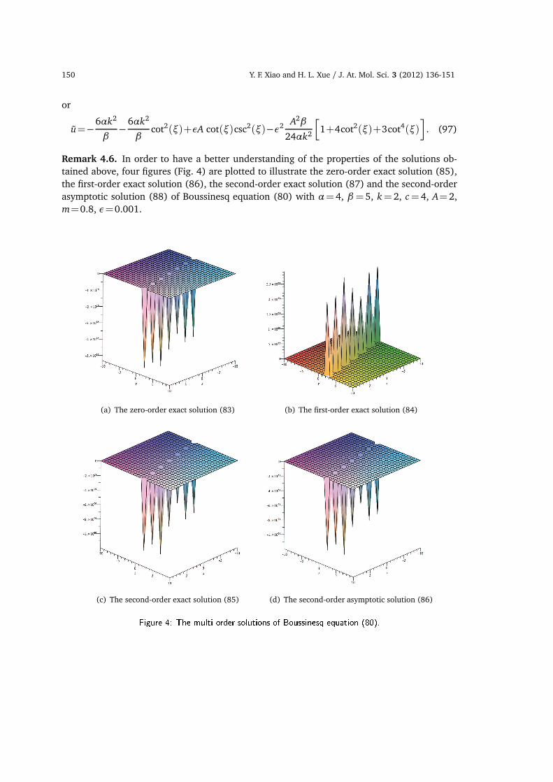
Remark 4.6. In order to have a better understanding of the properties of the solutions ob-
tained above, four figures (Fig. 4) are plotted to illustrate the zero-order exact solution (85),
the first-order exact solution (86), the second-order exact solution (87) and the second-order
asymptotic solution (88) of Boussinesq equation (80) with α=4, β=5, k=2, c=4, A=2,
m=0.8, ε=0.001.
(a) The zero-order exact solution (83) (b) The first-order exact solution (84)
(c) The second-order exact solution (85) (d) The second-order asymptotic solution (86)Figure 4: The multi-order solutions of Boussinesq equation (80).

Y. F. Xiao and H. L. Xue / J. At. Mol. Sci. 3 (2012) 136-151 151
5 Conclusion
In the paper, Jacobi elliptic function, the Lamé equation and Lamé functions are applied to
solve nonlinear evolution equations. When perturbation method and two kinds of the Lamé
functions L2(ξ) and L3(ξ) are considered, then the multi-order solutions are obtained for
these nonlinear evolution equations. The results obtained in the paper is very important for
nonlinear instability of nonlinear coherent structures of the nonlinear evolution equations.
Additionally the method can be also applied to many other nonlinear evolution equations in
mathematical physics.
Acknowledgments. The authors thanks the suggestions from referees and the support from
the Special Foundation for State Major Basic Research Program of China under Grant No.2004
CB318000 and the Young Scientists Fund of the National Natural Science Foundation of China
under Grant No.10901145.
References
[1] M. J. Ablowitz and P. A. Clarkson, Soliton, Nonlinear Evolution Equations and Inverse Scattering
(Cambridge University Press, New York, 1991).
[2] M. R. Miurs, Bäcklund Transformation (Springer, Berlin, 1978).
[3] C. H . Gu, H. S. Hu, and Z. X. Zhou, Darboux Transformation in Solitons Theory and its Geometry
Applications (Shanghai Science Technology Press, Shanghai, 1999).
[4] R. Hirota, Phys. Rev. Lett. 27 (1971) 1192.
[5] M. L. Wang, Phys. Lett. A 199(1996) 169.
[6] Z. L. Yan, X. Q. Liu, and L. Wang, Appl. Math. Computer 187 (2007) 701.
[7] C. T. Yan, Phys. Lett. A 224 (1996) 77.
[8] J. H. He, Chaos, Soliton and Fractals 26 (2005) 695.
[9] J. H. He, Phys. Lett. A 335(2005) 182.
[10] E. J. Parkes, B. R. Duffy, Comput. Phys. Commun. 98 (1996) 288.
[11] J. H. He and X. H. Wu, Chaos, Soliton and Fractals 30 (2006) 700.
[12] S. K. Liu, Z. T. Fu, S. D. Liu, and Q. Zhao, Phys. Lett. A 289 (2001) 69.
[13] Z. T. Fu, S. K. Liu, S. D. Liu, and Q. Zhao, Commun. Nonlinear Sci. Numerical Simulat. 8 (2003)
67.
[14] A. H. Nayfeh, Perturbation Methods (John Wiley and Sons, New York, 1973).
[15] S. K. Liu, Z. T. Fu, S. D. Liu, and Z. G. Wang, Chaos, Soliton and Fractals 19 (2004) 795.
[16] Z. T. Fu, N. M. Yuan, Z. Chen, J. Y. Mao, and S. K. Liu, Phys. Lett. A 373 (2009) 3710.
[17] Z. T. Fu, N. M. Yuan, J. Y. Mao, and S. K. Liu, Phys. Lett. A 374 (2009) 214.
[18] Z. X. Wang and D. R. Guo, Special Functions (World Scientific Press, Singapore, 1989).
[19] S. K. Liu and S. D. Liu, Nonlinear Equations in Physics (Peking University Press, Beijing, 2000).