the no-u-turn sampler: adaptively setting path lengths in

Journal of Machine Learning Research 15 (2014) 1351-1381 Submitted 11/11; Revised 10/13; Published 4/14

The No-U-Turn Sampler: Adaptively Setting Path Lengthsin Hamiltonian Monte Carlo

Matthew D. Hoffman [email protected] Research601 Townsend St.San Francisco, CA 94110, USA

Andrew Gelman [email protected]

Departments of Statistics and Political Science

Columbia University

New York, NY 10027, USA

Editor: Anthanasios Kottas

Abstract

Hamiltonian Monte Carlo (HMC) is a Markov chain Monte Carlo (MCMC) algorithm thatavoids the random walk behavior and sensitivity to correlated parameters that plague manyMCMC methods by taking a series of steps informed by first-order gradient information.These features allow it to converge to high-dimensional target distributions much morequickly than simpler methods such as random walk Metropolis or Gibbs sampling. However,HMC’s performance is highly sensitive to two user-specified parameters: a step size ε anda desired number of steps L. In particular, if L is too small then the algorithm exhibitsundesirable random walk behavior, while if L is too large the algorithm wastes computation.We introduce the No-U-Turn Sampler (NUTS), an extension to HMC that eliminates theneed to set a number of steps L. NUTS uses a recursive algorithm to build a set of likelycandidate points that spans a wide swath of the target distribution, stopping automaticallywhen it starts to double back and retrace its steps. Empirically, NUTS performs at least asefficiently as (and sometimes more efficiently than) a well tuned standard HMC method,without requiring user intervention or costly tuning runs. We also derive a method foradapting the step size parameter ε on the fly based on primal-dual averaging. NUTScan thus be used with no hand-tuning at all, making it suitable for applications such asBUGS-style automatic inference engines that require efficient “turnkey” samplers.

Keywords: Markov chain Monte Carlo, Hamiltonian Monte Carlo, Bayesian inference,adaptive Monte Carlo, dual averaging

1. Introduction

Hierarchical Bayesian models are a mainstay of the machine learning and statistics com-munities. Exact posterior inference in such models is rarely tractable, however, and soresearchers and practitioners must usually resort to approximate statistical inference meth-ods. Deterministic approximate inference algorithms (for example, those reviewed by Wain-wright and Jordan 2008) can be efficient, but introduce bias and can be difficult to applyto some models. Rather than computing a deterministic approximation to a target poste-rior (or other) distribution, Markov chain Monte Carlo (MCMC) methods offer schemes for

c©2014 Matthew D. Hoffman and Andrew Gelman.

Hoffman and Gelman

drawing a series of correlated samples that will converge in distribution to the target distri-bution (Neal, 1993). MCMC methods are sometimes less efficient than their deterministiccounterparts, but are more generally applicable and are asymptotically unbiased.

Not all MCMC algorithms are created equal. For complicated models with many param-eters, simple methods such as random-walk Metropolis (Metropolis et al., 1953) and Gibbssampling (Geman and Geman, 1984) may require an unacceptably long time to convergeto the target distribution. This is in large part due to the tendency of these methods toexplore parameter space via inefficient random walks (Neal, 1993). When model parametersare continuous rather than discrete, Hamiltonian Monte Carlo (HMC), also known as hybridMonte Carlo, is able to suppress such random walk behavior by means of a clever auxiliaryvariable scheme that transforms the problem of sampling from a target distribution into theproblem of simulating Hamiltonian dynamics (Neal, 2011). The cost of HMC per indepen-dent sample from a target distribution of dimension D is roughly O(D5/4), which stands insharp contrast with the O(D2) cost of random-walk Metropolis (Creutz, 1988).

HMC’s increased efficiency comes at a price. First, HMC requires the gradient of thelog-posterior. Computing the gradient for a complex model is at best tedious and at worstimpossible, but this requirement can be made less onerous by using automatic differentiation(Griewank and Walther, 2008). Second, HMC requires that the user specify at least twoparameters: a step size ε and a number of steps L for which to run a simulated Hamiltoniansystem. A poor choice of either of these parameters will result in a dramatic drop in HMC’sefficiency. Methods from the adaptive MCMC literature (see Andrieu and Thoms 2008 fora review) can be used to tune ε on the fly, but setting L typically requires one or morecostly tuning runs, as well as the expertise to interpret the results of those tuning runs.This hurdle limits the more widespread use of HMC, and makes it challenging to incorporateHMC into a general-purpose inference engine such as BUGS (Gilks and Spiegelhalter, 1992),JAGS (http://mcmc-jags.sourceforge.net), Infer.NET (Minka et al.), HBC (Daume III,2007), or PyMC (Patil et al., 2010).

The main contribution of this paper is the No-U-Turn Sampler (NUTS), an MCMCalgorithm that closely resembles HMC, but eliminates the need to choose the problematicnumber-of-steps parameter L. We also provide a new dual averaging (Nesterov, 2009)scheme for automatically tuning the step size parameter ε in both HMC and NUTS, makingit possible to run NUTS with no hand-tuning at all. We will show that the tuning-freeversion of NUTS samples as efficiently as (and sometimes more efficiently than) HMC, evenignoring the cost of finding optimal tuning parameters for HMC. Thus, NUTS brings theefficiency of HMC to users (and generic inference systems) that are unable or disinclined tospend time tweaking an MCMC algorithm.

Our algorithm has been implemented in C++ as part of the new open-source Bayesianinference package, Stan (Stan Development Team, 2013). Matlab code implementing thealgorithms, along with Stan code for models used in our simulation study, are also availableat http://www.cs.princeton.edu/~mdhoffma/.

2. Hamiltonian Monte Carlo

In Hamiltonian Monte Carlo (HMC) (Neal, 2011, 1993; Duane et al., 1987), we introduce anauxiliary momentum variable rd for each model variable θd. In the usual implementation,

1352

http://mcmc-jags.sourceforge.net

http://www.cs.princeton.edu/~mdhoffma/

The No-U-Turn Sampler

Algorithm 1 Hamiltonian Monte Carlo

Given θ0, ε, L, L,M :for m = 1 to M do

Sample r0 ∼ N (0, I).Set θm ← θm−1, θ ← θm−1, r ← r0.for i = 1 to L do

Set θ, r ← Leapfrog(θ, r, ε).end for

With probability α = min

{1,

exp{L(θ)− 12r·r}

exp{L(θm−1)− 12r0·r0}

}, set θm ← θ, rm ← −r.

end for

function Leapfrog(θ, r, ε)Set r ← r + (ε/2)∇θL(θ).Set θ ← θ + εr.Set r ← r + (ε/2)∇θL(θ).return θ, r.

these momentum variables are drawn independently from the standard normal distribution,yielding the (unnormalized) joint density

p(θ, r) ∝ exp{L(θ)− 12r · r},

where L is the logarithm of the joint density of the variables of interest θ (up to a normalizingconstant) and x · y denotes the inner product of the vectors x and y. We can interpret thisaugmented model in physical terms as a fictitious Hamiltonian system where θ denotes aparticle’s position in D-dimensional space, rd denotes the momentum of that particle inthe dth dimension, L is a position-dependent negative potential energy function, 1

2r · r isthe kinetic energy of the particle, and log p(θ, r) is the negative energy of the particle. Wecan simulate the evolution over time of the Hamiltonian dynamics of this system via theStormer-Verlet (“leapfrog”) integrator, which proceeds according to the updates

rt+ε/2 = rt + (ε/2)∇θL(θt); θt+ε = θt + εrt+ε/2; rt+ε = rt+ε/2 + (ε/2)∇θL(θt+ε),

where rt and θt denote the values of the momentum and position variables r and θ at timet and ∇θ denotes the gradient with respect to θ. Since the update for each coordinatedepends only on the other coordinates, the leapfrog updates are volume-preserving—thatis, the volume of a region remains unchanged after mapping each point in that region to anew point via the leapfrog integrator.

A standard procedure for drawing M samples via Hamiltonian Monte Carlo is describedin Algorithm 1. I denotes the identity matrix and N (µ,Σ) denotes a multivariate normaldistribution with mean µ and covariance matrix Σ. For each sample m, we first resamplethe momentum variables from a standard multivariate normal, which can be interpreted asa Gibbs sampling update. We then apply L leapfrog updates to the position and momentumvariables θ and r, generating a proposal position-momentum pair θ, r. We propose settingθm = θ and rm = −r, and accept or reject this proposal according to the Metropolis

1353

Hoffman and Gelman

algorithm (Metropolis et al., 1953). This is a valid Metropolis proposal because it is time-reversible and the leapfrog integrator is volume-preserving; using an algorithm for simulatingHamiltonian dynamics that did not preserve volume complicates the computation of theMetropolis acceptance probability (Lan et al., 2012). The negation of r in the proposal istheoretically necessary to produce time-reversibility, but can be omitted in practice if oneis only interested in sampling from p(θ).

The term log p(θ,r)p(θ,r) , on which the acceptance probability α depends, is the negative

change in energy of the simulated Hamiltonian system from time 0 to time εL. If we couldsimulate the Hamiltonian dynamics exactly, then α would always be 1, since energy is con-served in Hamiltonian systems. The error introduced by using a discrete-time simulation

depends on the step size parameter ε—specifically, the change in energy | log p(θ,r)p(θ,r) | is pro-

portional to ε2 for large L, or ε3 if L = 1 (Leimkuhler and Reich, 2004). In principle theerror can grow without bound as a function of L, but it typically does not due to the sym-plecticness of the leapfrog discretization. This allows us to run HMC with many leapfrogsteps, generating proposals for θ that have high probability of acceptance even though theyare distant from the previous sample.

The performance of HMC depends strongly on choosing suitable values for ε and L. Ifε is too large, then the simulation will be inaccurate and yield low acceptance rates. If εis too small, then computation will be wasted taking many small steps. If L is too small,then successive samples will be close to one another, resulting in undesirable random walkbehavior and slow mixing. If L is too large, then HMC will generate trajectories that loopback and retrace their steps. This is doubly wasteful, since work is being done to bring theproposal θ closer to the initial position θm−1. Worse, if L is chosen so that the parametersjump from one side of the space to the other each iteration, then the Markov chain maynot even be ergodic (Neal, 2011). More realistically, an unfortunate choice of L may resultin a chain that is ergodic but slow to move between regions of low and high density.

3. Eliminating the Need to Hand-Tune HMC

HMC is a powerful algorithm, but its usefulness is limited by the need to tune the step sizeparameter ε and number of steps L. Tuning these parameters for any particular problem re-quires some expertise, and usually one or more preliminary runs. Selecting L is particularlyproblematic; it is difficult to find a simple metric for when a trajectory is too short, too long,or “just right,” and so practitioners commonly rely on heuristics based on autocorrelationstatistics from preliminary runs (Neal, 2011).

Below, we present the No-U-Turn Sampler (NUTS), an extension of HMC that eliminatesthe need to specify a fixed value of L. In Section 3.2 we present schemes for setting ε basedon the dual averaging algorithm of Nesterov (2009).

3.1 No-U-Turn Hamiltonian Monte Carlo

Our first goal is to devise an MCMC sampler that retains HMC’s ability to suppress randomwalk behavior without the need to set the number L of leapfrog steps that the algorithmtakes to generate a proposal. We need some criterion to tell us when we have simulatedthe dynamics for “long enough,” that is, when running the simulation for more steps would

1354


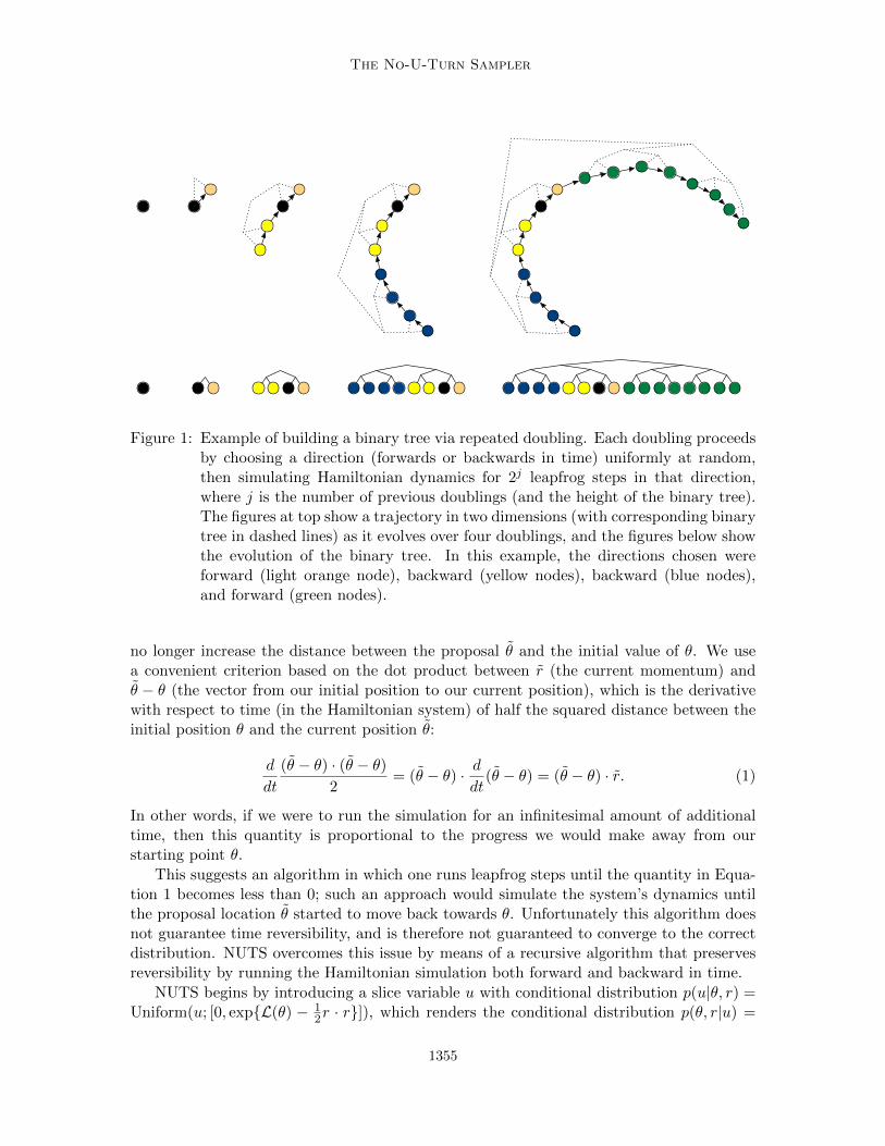
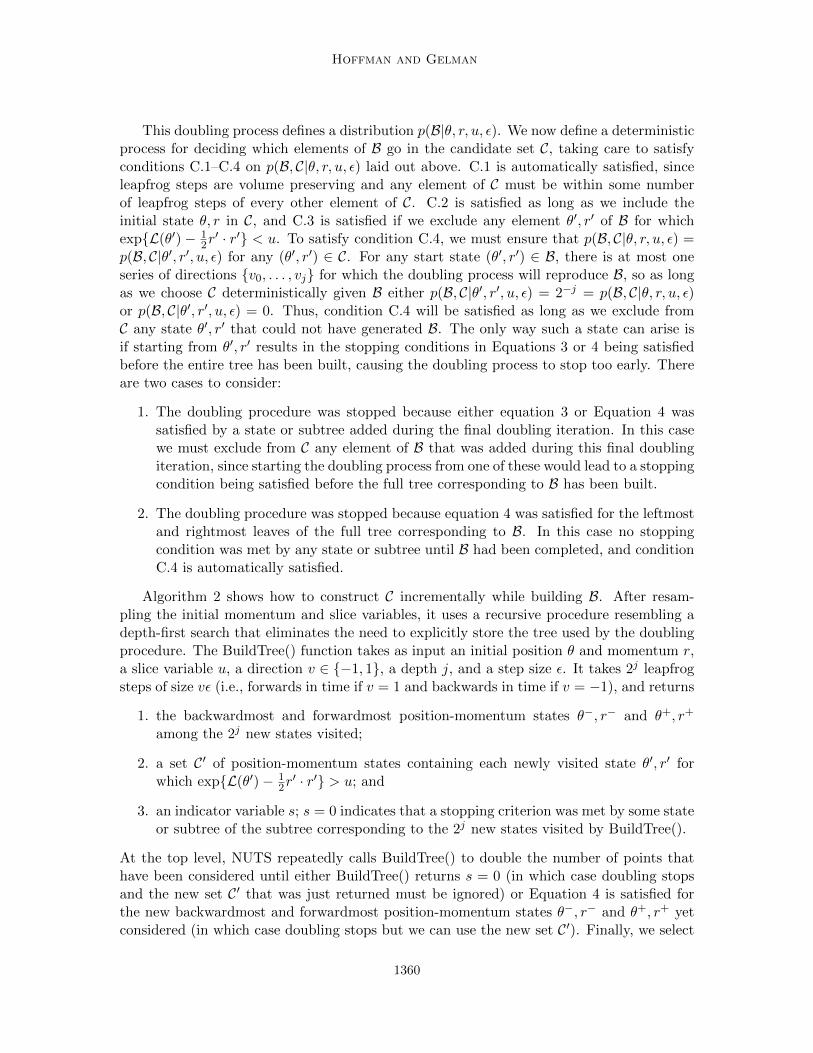
Figure 1: Example of building a binary tree via repeated doubling. Each doubling proceedsby choosing a direction (forwards or backwards in time) uniformly at random,then simulating Hamiltonian dynamics for 2j leapfrog steps in that direction,where j is the number of previous doublings (and the height of the binary tree).The figures at top show a trajectory in two dimensions (with corresponding binarytree in dashed lines) as it evolves over four doublings, and the figures below showthe evolution of the binary tree. In this example, the directions chosen wereforward (light orange node), backward (yellow nodes), backward (blue nodes),and forward (green nodes).

no longer increase the distance between the proposal θ and the initial value of θ. We usea convenient criterion based on the dot product between r (the current momentum) andθ − θ (the vector from our initial position to our current position), which is the derivativewith respect to time (in the Hamiltonian system) of half the squared distance between theinitial position θ and the current position θ:

d

dt

(θ − θ) · (θ − θ)2

= (θ − θ) · ddt

(θ − θ) = (θ − θ) · r. (1)

In other words, if we were to run the simulation for an infinitesimal amount of additionaltime, then this quantity is proportional to the progress we would make away from ourstarting point θ.

This suggests an algorithm in which one runs leapfrog steps until the quantity in Equa-tion 1 becomes less than 0; such an approach would simulate the system’s dynamics untilthe proposal location θ started to move back towards θ. Unfortunately this algorithm doesnot guarantee time reversibility, and is therefore not guaranteed to converge to the correctdistribution. NUTS overcomes this issue by means of a recursive algorithm that preservesreversibility by running the Hamiltonian simulation both forward and backward in time.

NUTS begins by introducing a slice variable u with conditional distribution p(u|θ, r) =Uniform(u; [0, exp{L(θ) − 1

2r · r}]), which renders the conditional distribution p(θ, r|u) =

1355

Hoffman and Gelman

−0.1 0 0.1 0.2 0.3 0.4 0.5

−0.1

0

0.1

0.2

0.3

0.4

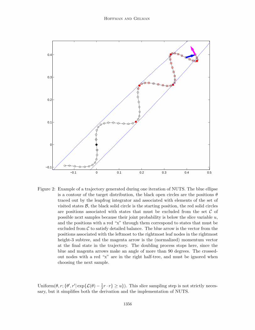
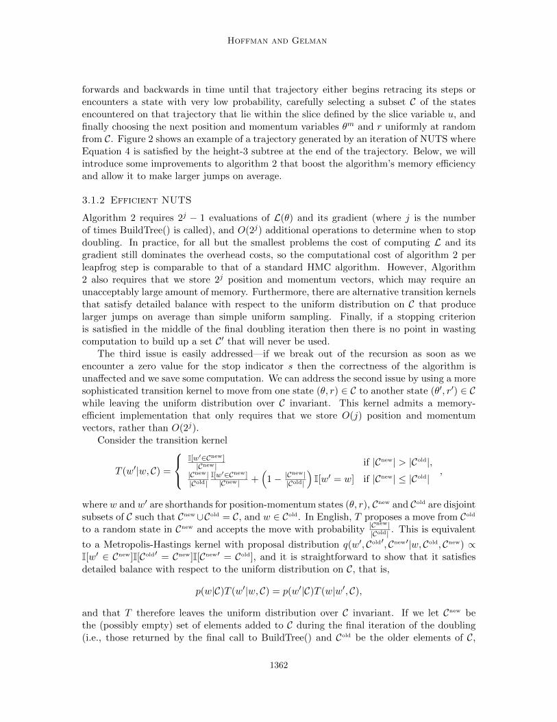
Figure 2: Example of a trajectory generated during one iteration of NUTS. The blue ellipseis a contour of the target distribution, the black open circles are the positions θtraced out by the leapfrog integrator and associated with elements of the set ofvisited states B, the black solid circle is the starting position, the red solid circlesare positions associated with states that must be excluded from the set C ofpossible next samples because their joint probability is below the slice variable u,and the positions with a red “x” through them correspond to states that must beexcluded from C to satisfy detailed balance. The blue arrow is the vector from thepositions associated with the leftmost to the rightmost leaf nodes in the rightmostheight-3 subtree, and the magenta arrow is the (normalized) momentum vectorat the final state in the trajectory. The doubling process stops here, since theblue and magenta arrows make an angle of more than 90 degrees. The crossed-out nodes with a red “x” are in the right half-tree, and must be ignored whenchoosing the next sample.

Uniform(θ, r; {θ′, r′| exp{L(θ)− 12r · r} ≥ u}). This slice sampling step is not strictly neces-

sary, but it simplifies both the derivation and the implementation of NUTS.

1356


At a high level, after resampling u|θ, r, NUTS uses the leapfrog integrator to trace out apath forwards and backwards in fictitious time, first running forwards or backwards 1 step,then forwards or backwards 2 steps, then forwards or backwards 4 steps, etc. This doublingprocess implicitly builds a balanced binary tree whose leaf nodes correspond to position-momentum states, as illustrated in Figure 1. The doubling is halted when the subtrajectoryfrom the leftmost to the rightmost nodes of any balanced subtree of the overall binary treestarts to double back on itself (i.e., the fictional particle starts to make a “U-turn”). Atthis point NUTS stops the simulation and samples from among the set of points computedduring the simulation, taking care to preserve detailed balance. Figure 2 illustrates anexample of a trajectory computed during an iteration of NUTS.

Pseudocode implementing a efficient version of NUTS is provided in Algorithm 3. Adetailed derivation follows below, along with a simplified version of the algorithm thatmotivates and builds intuition about Algorithm 3 (but uses much more memory and makessmaller jumps).

3.1.1 Derivation of Simplified NUTS Algorithm

NUTS further augments the model p(θ, r) ∝ exp{L(θ)− 12r ·r} with a slice variable u (Neal,

2003). The joint probability of θ, r, and u is

p(θ, r, u) ∝ I[u ∈ [0, exp{L(θ)− 12r · r}]],

where I[·] is 1 if the expression in brackets is true and 0 if it is false. The (unnormalized)marginal probability of θ and r (integrating over u) is

p(θ, r) ∝ exp{L(θ)− 12r · r},

as in standard HMC. The conditional probabilities p(u|θ, r) and p(θ, r|u) are each uniform,so long as the condition u ≤ exp{L(θ)− 1

2r · r} is satisfied.We also add a finite set C of candidate position-momentum states and another finite set

B ⊇ C to the model. B will be the set of all position-momentum states that the leapfrogintegrator traces out during a given NUTS iteration, and C will be the subset of thosestates to which we can transition without violating detailed balance. B will be built up byrandomly taking forward and backward leapfrog steps, and C will selected deterministicallyfrom B. The random procedure for building B and C given θ, r, u, and ε will define aconditional distribution p(B, C|θ, r, u, ε), upon which we place the following conditions:

C.1: All elements of C must be chosen in a way that preserves volume. That is, anydeterministic transformations of θ, r used to add a state θ′, r′ to C must have a Jacobianwith unit determinant.

C.2: p((θ, r) ∈ C|θ, r, u, ε) = 1.

C.3: p(u ≤ exp{L(θ′)− 12r′ · r′}|(θ′, r′) ∈ C) = 1.

C.4: If (θ, r) ∈ C and (θ′, r′) ∈ C then for any B, p(B, C|θ, r, u, ε) = p(B, C|θ′, r′, u, ε).

C.1 ensures that p(θ, r|(θ, r) ∈ C) ∝ p(θ, r), that is, if we restrict our attention to theelements of C then we can treat the unnormalized probability density of a particular element

1357

Hoffman and Gelman

of C as an unnormalized probability mass. C.2 says that the current state θ, r must beincluded in C. C.3 requires that any state in C be in the slice defined by u, that is, that anystate (θ′, r′) ∈ C must have equal (and positive) conditional probability density p(θ′, r′|u).C.4 states that B and C must have equal probability of being selected regardless of thecurrent state θ, r as long as (θ, r) ∈ C (which it must be by C.2).

Deferring for the moment the question of how to construct and sample from a distribu-tion p(B, C|θ, r, u, ε) that satisfies these conditions, we will now show that the the followingprocedure leaves the joint distribution p(θ, r, u,B, C|ε) invariant:

1. sample r ∼ N (0, I),

2. sample u ∼ Uniform([0, exp{L(θt)− 12r · r}]),

3. sample B, C from their conditional distribution p(B, C|θt, r, u, ε),

4. sample θt+1, r ∼ T (θt, r, C),

where T (θ′, r′|θ, r, C) is a transition kernel that leaves the uniform distribution over C in-variant, that is, T must satisfy

1

|C|∑

(θ,r)∈C

T (θ′, r′|θ, r, C) =I[(θ′, r′) ∈ C]

|C|

for any θ′, r′. The notation θt+1, r ∼ T (θt, r, C) denotes that we are resampling r in a waythat depends on its current value.

Steps 1, 2, and 3 resample r, u, B, and C from their conditional joint distribution givenθt, and therefore together constitute a valid Gibbs sampling update. Step 4 is valid becausethe joint distribution of θ and r given u,B, C, and ε is uniform on the elements of C:

p(θ, r|u,B, C, ε) ∝ p(B, C|θ, r, u, ε)p(θ, r|u)

∝ p(B, C|θ, r, u, ε)I[u ≤ exp{L(θ)− 12r · r}]

∝ I[(θ, r) ∈ C].(2)

Condition C.1 allows us to treat the unnormalized conditional density p(θ, r|u) ∝ I[u ≤exp{L(θ) − 1

2r · r}] as an unnormalized conditional probability mass function. ConditionsC.2 and C.4 ensure that p(B, C|θ, r, u, ε) ∝ I[(θ, r) ∈ C] because by C.2 (θ, r) must be in C,and by C.4 for any B, C pair p(B, C|θ, r, u, ε) is constant as a function of θ and r as long as(θ, r) ∈ C. Condition C.3 ensures that (θ, r) ∈ C ⇒ u ≤ exp{L(θ)− 1

2r ·r} (so the p(θ, r|u, ε)term is redundant). Thus, Equation 2 implies that the joint distribution of θ and r given uand C is uniform on the elements of C, and we are free to choose a new θt+1, rt+1 from anytransition kernel that leaves this uniform distribution on C invariant.

We now turn our attention to the specific form for p(B, C|θ, r, u, ε) used by NUTS.Conceptually, the generative process for building B proceeds by repeatedly doubling thesize of a binary tree whose leaves correspond to position-momentum states. These stateswill constitute the elements of B. The initial tree has a single node corresponding to theinitial state. Doubling proceeds by choosing a random direction vj ∼ Uniform({−1, 1}) andtaking 2j leapfrog steps of size vjε (i.e., forwards in fictional time if vj = 1 and backwards in

1358


fictional time if vj = −1), where j is the current height of the tree. (The initial single-nodetree is defined to have height 0.) For example, if vj = 1, the left half of the new tree is theold tree and the right half of the new tree is a balanced binary tree of height j whose leafnodes correspond to the 2j position-momentum states visited by the new leapfrog trajectory.This doubling process is illustrated in Figure 1. Given the initial state θ, r and the step sizeε, there are 2j possible trees of height j that can be built according to this procedure, eachof which is equally likely. Conversely, the probability of reconstructing a particular tree ofheight j starting from any leaf node of that tree is 2−j regardless of which leaf node westart from.1

We cannot keep expanding the tree forever, of course. We want to continue expanding Buntil one end of the trajectory we are simulating makes a “U-turn” and begins to loop backtowards another position on the trajectory. At that point continuing the simulation is likelyto be wasteful, since the trajectory will retrace its steps and visit locations in parameterspace close to those we have already visited. We also want to stop expanding B if theerror in the simulation becomes extremely large, indicating that any states discovered bycontinuing the simulation longer are likely to have astronomically low probability. (Thismay happen if we use a step size ε that is too large, or if the target distribution includeshard constraints that make the log-density L go to −∞ in some regions.)

The second rule is easy to formalize—we simply stop doubling if the tree includes a leafnode whose state θ, r satisfies

L(θ)− 1

2r · r − log u < −∆max (3)

for some nonnegative ∆max. We recommend setting ∆max to a large value like 1000 sothat it does not interfere with the algorithm so long as the simulation is even moderatelyaccurate.

We must be careful when defining the first rule so that we can build a sampler thatneither violates detailed balance nor introduces excessive computational overhead. To de-termine whether to stop doubling the tree at height j, NUTS considers the 2j − 1 balancedbinary subtrees of the height-j tree that have height greater than 0. NUTS stops the dou-bling process when for one of these subtrees the states θ−, r− and θ+, r+ associated withthe leftmost and rightmost leaves of that subtree satisfies

(θ+ − θ−) · r− < 0 or (θ+ − θ−) · r+ < 0. (4)

That is, we stop if continuing the simulation an infinitesimal amount either forward or back-ward in time would reduce the distance between the position vectors θ− and θ+. Evaluatingthe condition in Equation 4 for each balanced subtree of a tree of height j requires 2j+1− 2inner products, which is comparable to the number of inner products required by the 2j −1leapfrog steps needed to compute the trajectory. Except for very simple models with verylittle data, the cost of these inner products should be negligible compared to the cost ofcomputing gradients.

1. This procedure resembles the doubling procedure devised by Neal (2003) to update scalar variables in away that leaves their conditional distribution invariant. The doubling procedure finds a set of candidatepoints by repeatedly doubling the size of a segment of the real line containing the initial point. NUTS,by contrast, repeatedly doubles the size of a finite candidate set of vectors that contains the initial state.

1359

Hoffman and Gelman

This doubling process defines a distribution p(B|θ, r, u, ε). We now define a deterministicprocess for deciding which elements of B go in the candidate set C, taking care to satisfyconditions C.1–C.4 on p(B, C|θ, r, u, ε) laid out above. C.1 is automatically satisfied, sinceleapfrog steps are volume preserving and any element of C must be within some numberof leapfrog steps of every other element of C. C.2 is satisfied as long as we include theinitial state θ, r in C, and C.3 is satisfied if we exclude any element θ′, r′ of B for whichexp{L(θ′)− 1

2r′ · r′} < u. To satisfy condition C.4, we must ensure that p(B, C|θ, r, u, ε) =

p(B, C|θ′, r′, u, ε) for any (θ′, r′) ∈ C. For any start state (θ′, r′) ∈ B, there is at most oneseries of directions {v0, . . . , vj} for which the doubling process will reproduce B, so as longas we choose C deterministically given B either p(B, C|θ′, r′, u, ε) = 2−j = p(B, C|θ, r, u, ε)or p(B, C|θ′, r′, u, ε) = 0. Thus, condition C.4 will be satisfied as long as we exclude fromC any state θ′, r′ that could not have generated B. The only way such a state can arise isif starting from θ′, r′ results in the stopping conditions in Equations 3 or 4 being satisfiedbefore the entire tree has been built, causing the doubling process to stop too early. Thereare two cases to consider:

1. The doubling procedure was stopped because either equation 3 or Equation 4 wassatisfied by a state or subtree added during the final doubling iteration. In this casewe must exclude from C any element of B that was added during this final doublingiteration, since starting the doubling process from one of these would lead to a stoppingcondition being satisfied before the full tree corresponding to B has been built.

2. The doubling procedure was stopped because equation 4 was satisfied for the leftmostand rightmost leaves of the full tree corresponding to B. In this case no stoppingcondition was met by any state or subtree until B had been completed, and conditionC.4 is automatically satisfied.

Algorithm 2 shows how to construct C incrementally while building B. After resam-pling the initial momentum and slice variables, it uses a recursive procedure resembling adepth-first search that eliminates the need to explicitly store the tree used by the doublingprocedure. The BuildTree() function takes as input an initial position θ and momentum r,a slice variable u, a direction v ∈ {−1, 1}, a depth j, and a step size ε. It takes 2j leapfrogsteps of size vε (i.e., forwards in time if v = 1 and backwards in time if v = −1), and returns

1. the backwardmost and forwardmost position-momentum states θ−, r− and θ+, r+

among the 2j new states visited;

2. a set C′ of position-momentum states containing each newly visited state θ′, r′ forwhich exp{L(θ′)− 1

2r′ · r′} > u; and

3. an indicator variable s; s = 0 indicates that a stopping criterion was met by some stateor subtree of the subtree corresponding to the 2j new states visited by BuildTree().

At the top level, NUTS repeatedly calls BuildTree() to double the number of points thathave been considered until either BuildTree() returns s = 0 (in which case doubling stopsand the new set C′ that was just returned must be ignored) or Equation 4 is satisfied forthe new backwardmost and forwardmost position-momentum states θ−, r− and θ+, r+ yetconsidered (in which case doubling stops but we can use the new set C′). Finally, we select

1360


Algorithm 2 Naive No-U-Turn Sampler

Given θ0, ε, L, M :for m = 1 to M do

Resample r0 ∼ N (0, I).Resample u ∼ Uniform([0, exp{L(θm−1 − 1

2r0 · r0}])

Initialize θ− = θm−1, θ+ = θm−1, r− = r0, r+ = r0, j = 0, C = {(θm−1, r0)}, s = 1.while s = 1 do

Choose a direction vj ∼ Uniform({−1, 1}).if vj = −1 thenθ−, r−,−,−, C′, s′ ← BuildTree(θ−, r−, u, vj , j, ε).

else−,−, θ+, r+, C′, s′ ← BuildTree(θ+, r+, u, vj , j, ε).

end ifif s′ = 1 thenC ← C ∪ C′.

end ifs← s′I[(θ+ − θ−) · r− ≥ 0]I[(θ+ − θ−) · r+ ≥ 0].j ← j + 1.

end whileSample θm, r uniformly at random from C.

end for

function BuildTree(θ, r, u, v, j, ε)if j = 0 then

Base case—take one leapfrog step in the direction v.θ′, r′ ← Leapfrog(θ, r, vε).

C′ ←{{(θ′, r′)} if u ≤ exp{L(θ′)− 1

2r′ · r′}

∅ else

s′ ← I[L(θ′)− 12r′ · r′ > log u−∆max].

return θ′, r′, θ′, r′, C′, s′.else

Recursion—build the left and right subtrees.θ−, r−, θ+, r+, C′, s′ ← BuildTree(θ, r, u, v, j − 1, ε).if v = −1 thenθ−, r−,−,−, C′′, s′′ ← BuildTree(θ−, r−, u, v, j − 1, ε).

else−,−, θ+, r+, C′′, s′′ ← BuildTree(θ+, r+, u, v, j − 1, ε).

end ifs′ ← s′s′′I[(θ+ − θ−) · r− ≥ 0]I[(θ+ − θ−) · r+ ≥ 0].C′ ← C′ ∪ C′′.return θ−, r−, θ+, r+, C′, s′.

end if

the next position and momentum θm, r uniformly at random from C, the union of all of thevalid sets C′ that have been returned, which clearly leaves the uniform distribution over Cinvariant.

To summarize, Algorithm 2 defines a transition kernel that leaves p(θ, r, u,B, C|ε) invari-ant, and therefore leaves the target distribution p(θ) ∝ exp{L(θ)} invariant. It does so byresampling the momentum and slice variables r and u, simulating a Hamiltonian trajectory

1361

Hoffman and Gelman

forwards and backwards in time until that trajectory either begins retracing its steps orencounters a state with very low probability, carefully selecting a subset C of the statesencountered on that trajectory that lie within the slice defined by the slice variable u, andfinally choosing the next position and momentum variables θm and r uniformly at randomfrom C. Figure 2 shows an example of a trajectory generated by an iteration of NUTS whereEquation 4 is satisfied by the height-3 subtree at the end of the trajectory. Below, we willintroduce some improvements to algorithm 2 that boost the algorithm’s memory efficiencyand allow it to make larger jumps on average.

3.1.2 Efficient NUTS

Algorithm 2 requires 2j − 1 evaluations of L(θ) and its gradient (where j is the numberof times BuildTree() is called), and O(2j) additional operations to determine when to stopdoubling. In practice, for all but the smallest problems the cost of computing L and itsgradient still dominates the overhead costs, so the computational cost of algorithm 2 perleapfrog step is comparable to that of a standard HMC algorithm. However, Algorithm2 also requires that we store 2j position and momentum vectors, which may require anunacceptably large amount of memory. Furthermore, there are alternative transition kernelsthat satisfy detailed balance with respect to the uniform distribution on C that producelarger jumps on average than simple uniform sampling. Finally, if a stopping criterionis satisfied in the middle of the final doubling iteration then there is no point in wastingcomputation to build up a set C′ that will never be used.

The third issue is easily addressed—if we break out of the recursion as soon as weencounter a zero value for the stop indicator s then the correctness of the algorithm isunaffected and we save some computation. We can address the second issue by using a moresophisticated transition kernel to move from one state (θ, r) ∈ C to another state (θ′, r′) ∈ Cwhile leaving the uniform distribution over C invariant. This kernel admits a memory-efficient implementation that only requires that we store O(j) position and momentumvectors, rather than O(2j).

Consider the transition kernel

T (w′|w, C) =

I[w′∈Cnew]|Cnew| if |Cnew| > |Cold|,

|Cnew||Cold|

I[w′∈Cnew]|Cnew| +

(1− |C

new||Cold|

)I[w′ = w] if |Cnew| ≤ |Cold|

,

where w and w′ are shorthands for position-momentum states (θ, r), Cnew and Cold are disjointsubsets of C such that Cnew∪Cold = C, and w ∈ Cold. In English, T proposes a move from Cold

to a random state in Cnew and accepts the move with probability |Cnew||Cold| . This is equivalent

to a Metropolis-Hastings kernel with proposal distribution q(w′, Cold′, Cnew′|w, Cold, Cnew) ∝I[w′ ∈ Cnew]I[Cold′ = Cnew]I[Cnew′ = Cold], and it is straightforward to show that it satisfiesdetailed balance with respect to the uniform distribution on C, that is,

p(w|C)T (w′|w, C) = p(w′|C)T (w|w′, C),

and that T therefore leaves the uniform distribution over C invariant. If we let Cnew bethe (possibly empty) set of elements added to C during the final iteration of the doubling(i.e., those returned by the final call to BuildTree() and Cold be the older elements of C,

1362


then we can replace the uniform sampling of C at the end of Algorithm 2 with a drawfrom T (θt, rt, C) and leave the uniform distribution on C invariant. In fact, we can apply Tafter every doubling, proposing a move to each new half-tree in turn. Doing so leaves theuniform distribution on each partially built C invariant, and therefore does no harm to theinvariance of the uniform distribution on the fully built set C. Repeatedly applying T inthis way increases the probability that we will jump to a state θt+1 far from the initial stateθt; considering the process in reverse, it is as though we first tried to jump to the otherside of C, then if that failed tried to make a more modest jump, and so on. This transitionkernel is thus akin to delayed-rejection MCMC methods (Tierney and Mira, 1999), but inthis setting we can avoid the usual costs associated with evaluating new proposals.

The transition kernel above still requires that we be able to sample uniformly from theset C′ returned by BuildTree(), which may contain as many as 2j−1 elements. In fact, wecan sample from C′ without maintaining the full set C′ in memory by exploiting the binarytree structure in Figure 1. Consider a subtree of the tree explored in a call to BuildTree(),and let Csubtree denote the set of its leaf states that are in C′: we can factorize the probabilitythat a state (θ, r) ∈ Csubtree will be chosen uniformly at random from C′ as

p(θ, r|C′) =1

|C′|=|Csubtree||C′|

1

|Csubtree|= p((θ, r) ∈ Csubtree|C)p(θ, r|(θ, r) ∈ Csubtree, C).

That is, p(θ, r|C′) is the product of the probability of choosing some node from the subtreemultiplied by the probability of choosing θ, r uniformly at random from Csubtree. We usethis observation to sample from C′ incrementally as we build up the tree. Each subtreeabove the bottom layer is built of two smaller subtrees. For each of these smaller subtrees,we sample a θ, r pair from p(θ, r|(θ, r) ∈ Csubtree) to represent that subtree. We then choosebetween these two pairs, giving the pair representing each subtree weight proportional tohow many elements of C′ are in that subtree. This continues until we have completed thesubtree associated with C′ and we have returned a sample θ′ from C′ and an integer weightn′ encoding the size of C′, which is all we need to apply T . This procedure only requires thatwe store O(j) position and momentum vectors in memory, rather than O(2j), and requiresthat we generate O(2j) extra random numbers (a cost that again is usually very smallcompared with the 2j − 1 gradient computations needed to run the leapfrog algorithm).

Algorithm 3 implements all of the above improvements in pseudocode.

3.2 Adaptively Tuning ε

Having addressed the issue of how to choose the number of steps L, we now turn ourattention to the step size parameter ε. To set ε for both NUTS and HMC, we propose usingstochastic optimization with vanishing adaptation (Andrieu and Thoms, 2008), specificallyan adaptation of the primal-dual algorithm of Nesterov (2009).

Perhaps the most commonly used vanishing adaptation algorithm in MCMC is thestochastic approximation method of Robbins and Monro (1951). Suppose we have a statisticHt that describes some aspect of the behavior of an MCMC algorithm at iteration t ≥ 1,

1363

Hoffman and Gelman

Algorithm 3 Efficient No-U-Turn Sampler

Given θ0, ε, L, M :for m = 1 to M do

Resample r0 ∼ N (0, I).Resample u ∼ Uniform([0, exp{L(θm−1 − 1

2r0 · r0}])

Initialize θ− = θm−1, θ+ = θm−1, r− = r0, r+ = r0, j = 0, θm = θm−1, n = 1, s = 1.while s = 1 do

Choose a direction vj ∼ Uniform({−1, 1}).if vj = −1 thenθ−, r−,−,−, θ′, n′, s′ ← BuildTree(θ−, r−, u, vj , j, ε).

else−,−, θ+, r+, θ′, n′, s′ ← BuildTree(θ+, r+, u, vj , j, ε).

end ifif s′ = 1 then

With probability min{1, n′

n }, set θm ← θ′.end ifn← n+ n′.s← s′I[(θ+ − θ−) · r− ≥ 0]I[(θ+ − θ−) · r+ ≥ 0].j ← j + 1.

end whileend for

function BuildTree(θ, r, u, v, j, ε)if j = 0 then

Base case—take one leapfrog step in the direction v.θ′, r′ ← Leapfrog(θ, r, vε).n′ ← I[u ≤ exp{L(θ′)− 1

2r′ · r′}].

s′ ← I[L(θ′)− 12r′ · r′ > log u−∆max]

return θ′, r′, θ′, r′, θ′, n′, s′.else

Recursion—implicitly build the left and right subtrees.θ−, r−, θ+, r+, θ′, n′, s′ ← BuildTree(θ, r, u, v, j − 1, ε).if s′ = 1 then

if v = −1 thenθ−, r−,−,−, θ′′, n′′, s′′ ← BuildTree(θ−, r−, u, v, j − 1, ε).

else−,−, θ+, r+, θ′′, n′′, s′′ ← BuildTree(θ+, r+, u, v, j − 1, ε).

end ifWith probability n′′

n′+n′′ , set θ′ ← θ′′.

s′ ← s′′I[(θ+ − θ−) · r− ≥ 0]I[(θ+ − θ−) · r+ ≥ 0]n′ ← n′ + n′′

end ifreturn θ−, r−, θ+, r+, θ′, n′, s′.

end if

and define its expectation h(x) as

h(x) ≡ Et[Ht|x] ≡ limT→∞

1

T

T∑t=1

E[Ht|x],

1364


where x ∈ R is a tunable parameter to the MCMC algorithm. For example, if αt is theMetropolis acceptance probability for iteration t, we might define Ht = δ − αt, where δ isthe desired average acceptance probability. If h is a nondecreasing function of x and a fewother conditions such as boundedness of the iterates xt are met (see Andrieu and Thoms2008 for details), the update

xt+1 ← xt − ηtHt

is guaranteed to cause h(xt) to converge to 0 as long as the step size schedule defined by ηtsatisfies the conditions ∑

t

ηt =∞;∑t

η2t <∞. (5)

These conditions are satisfied by schedules of the form ηt ≡ t−κ for κ ∈ (0.5, 1]. As long asthe per-iteration impact of the adaptation goes to 0 (as it will if ηt ≡ t−κ and κ > 0) theasymptotic behavior of the sampler is unchanged. That said, in practice x often gets “closeenough” to an optimal value well before the step size η has gotten close enough to 0 to avoiddisturbing the Markov chain’s stationary distribution. A common practice, which we followhere, is to adapt any tunable MCMC parameters during the warmup phase, and freeze thetunable parameters afterwards (e.g., Gelman et al., 2004). For the present paper, the stepsize ε is the only tuning parameter x in the algorithm. More advanced implementationscould have more options, though, so we consider the tuning problem more generally.

3.2.1 Dual Averaging

The optimal values of the parameters to an MCMC algorithm during the warmup phaseand the stationary phase are often quite different. Ideally those parameters would thereforeadapt quickly as we shift from the sampler’s initial, transient regime to its stationary regime.However, the diminishing step sizes of Robbins-Monro give disproportionate weight to theearly iterations, which is the opposite of what we want.

Similar issues motivate the dual averaging scheme of Nesterov (2009), an algorithmfor nonsmooth and stochastic convex optimization. Since solving an unconstrained con-vex optimization problem is equivalent to finding a zero of a nondecreasing function (the(sub)gradient of the cost function), it is straightforward to adapt dual averaging to the prob-lem of MCMC adaptation by replacing stochastic gradients with the statistics Ht. Againassuming that we want to find a setting of a parameter x ∈ R such that h(x) ≡ Et[Ht|x] = 0,we can apply the updates

xt+1 ← µ−√t

γ

1

t+ t0

t∑i=1

Hi; xt+1 ← ηtxt+1 + (1− ηt)xt, (6)

where µ is a freely chosen point that the iterates xt are shrunk towards, γ > 0 is a freeparameter that controls the amount of shrinkage towards µ, t0 ≥ 0 is a free parameter thatstabilizes the initial iterations of the algorithm, ηt ≡ t−κ is a step size schedule obeying theconditions in Equation 5, and we define x1 = x1. As in Robbins-Monro, the per-iterationimpact of these updates on x goes to 0 as t goes to infinity. Specifically, for large t we have

xt+1 − xt = O(−Htt−0.5),

1365

Hoffman and Gelman

which clearly goes to 0 as long as the statistic Ht is bounded. The sequence of averagediterates xt is guaranteed to converge to a value such that h(xt) converges to 0.

The update scheme in Equation 6 is slightly more elaborate than the update schemeof Nesterov (2009), which implicitly has t0 ≡ 0 and κ ≡ 1. Introducing these parametersaddresses issues that are more important in MCMC adaptation than in more conventionalstochastic convex optimization settings. Setting t0 > 0 improves the stability of the algo-rithm in early iterations, which prevents us from wasting computation by trying out extremevalues. This is particularly important for NUTS, and for HMC when simulation lengths arespecified in terms of the overall simulation length εL instead of a fixed number of steps L.In both of these cases, lower values of ε result in more work being done per sample, so wewant to avoid casually trying out extremely low values of ε. Setting the parameter κ < 1allows us to give higher weight to more recent iterates and more quickly forget the iteratesproduced during the early warmup stages. The benefits of introducing these parameters areless apparent in the settings originally considered by Nesterov, where the cost of a stochasticgradient computation is assumed to be constant and the stochastic gradients are assumedto be drawn i.i.d. given the parameter x.

Allowing t0 > 0 and κ ∈ (0.5, 1] does not affect the asymptotic convergence of the dualaveraging algorithm. For any κ ∈ (0.5, 1], xt will eventually converge to the same value1t

∑ti=1 xt. We can rewrite the term

√tγ

1t+t0

as t√t

γ(t+t0)1t ;

t√t

γ(t+t0) is still O(√t), which is the

only feature needed to guarantee convergence.

We used the values γ = 0.05, t0 = 10, and κ = 0.75 for all our experiments. We arrivedat these values by trying a few settings for each parameter by hand with NUTS and HMC(with simulation lengths specified in terms of εL) on the stochastic volatility model describedbelow and choosing a value for each parameter that seemed to produce reasonable behavior.Better results might be obtained with further tweaking, but these default parameters seemto work consistently well for both NUTS and HMC for all of the models that we tested. Itis entirely possible that these parameter settings may not work as well for other samplingalgorithms or for H statistics other than the ones described below.

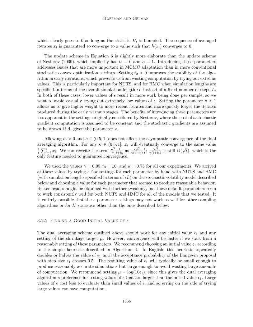
3.2.2 Finding a Good Initial Value of ε

The dual averaging scheme outlined above should work for any initial value ε1 and anysetting of the shrinkage target µ. However, convergence will be faster if we start from areasonable setting of these parameters. We recommend choosing an initial value ε1 accordingto the simple heuristic described in Algorithm 4. In English, this heuristic repeatedlydoubles or halves the value of ε1 until the acceptance probability of the Langevin proposalwith step size ε1 crosses 0.5. The resulting value of ε1 will typically be small enough toproduce reasonably accurate simulations but large enough to avoid wasting large amountsof computation. We recommend setting µ = log(10ε1), since this gives the dual averagingalgorithm a preference for testing values of ε that are larger than the initial value ε1. Largevalues of ε cost less to evaluate than small values of ε, and so erring on the side of tryinglarge values can save computation.

1366


3.2.3 Setting ε in HMC

In HMC we want to find a value for the step size ε that is neither too small (which wouldwaste computation by taking needlessly tiny steps) nor too large (which would waste com-putation by causing high rejection rates). A standard approach is to tune ε so that HMC’saverage Metropolis acceptance probability is equal to some value δ. Indeed, it has beenshown that (under fairly strong assumptions) the optimal value of ε for a given simulationlength εL is the one that produces an average Metropolis acceptance probability of approx-imately 0.65 (Beskos et al., 2010; Neal, 2011). For HMC, we define a criterion hHMC(ε) sothat

HHMCt ≡ min

{1,

p(θt, rt)

p(θt−1, rt,0)

}; hHMC(ε) ≡ Et[HHMC

t |ε],

where θt and rt are the proposed position and momentum at the tth iteration of the Markovchain, θt−1 and rt,0 are the initial position and (resampled) momentum for the tth iterationof the Markov chain, HHMC

t is the acceptance probability of this tth HMC proposal andhHMC is the expected average acceptance probability of the chain in equilibrium for a fixedε. Assuming that hHMC is nonincreasing as a function of ε, we can apply the updates inEquation 6 with Ht ≡ δ −HHMC

t and x ≡ log ε to coerce hHMC = δ for any δ ∈ (0, 1).

3.2.4 Setting ε in NUTS

Since there is no single accept/reject step in NUTS we must define an alternative statisticto Metropolis acceptance probability. For each iteration we define the statistic HNUTS

t andits expectation when the chain has reached equilibrium as

HNUTSt ≡ 1

|Bfinalt |

∑θ,r∈Bfinal

t

min

{1,

p(θ, r)

p(θt−1, rt,0)

}; hNUTS ≡ Et[HNUTS

t ],

where Bfinalt is the set of all states explored during the final doubling of iteration t of the

Markov chain and θt−1 and rt,0 are the initial position and (resampled) momentum for thetth iteration of the Markov chain. HNUTS can be understood as the average acceptanceprobability that HMC would give to the position-momentum states explored during thefinal doubling iteration. As above, assuming that HNUTS is nonincreasing in ε, we canapply the updates in Equation 6 with Ht ≡ δ −HNUTS and x ≡ log ε to coerce hNUTS = δfor any δ ∈ (0, 1).

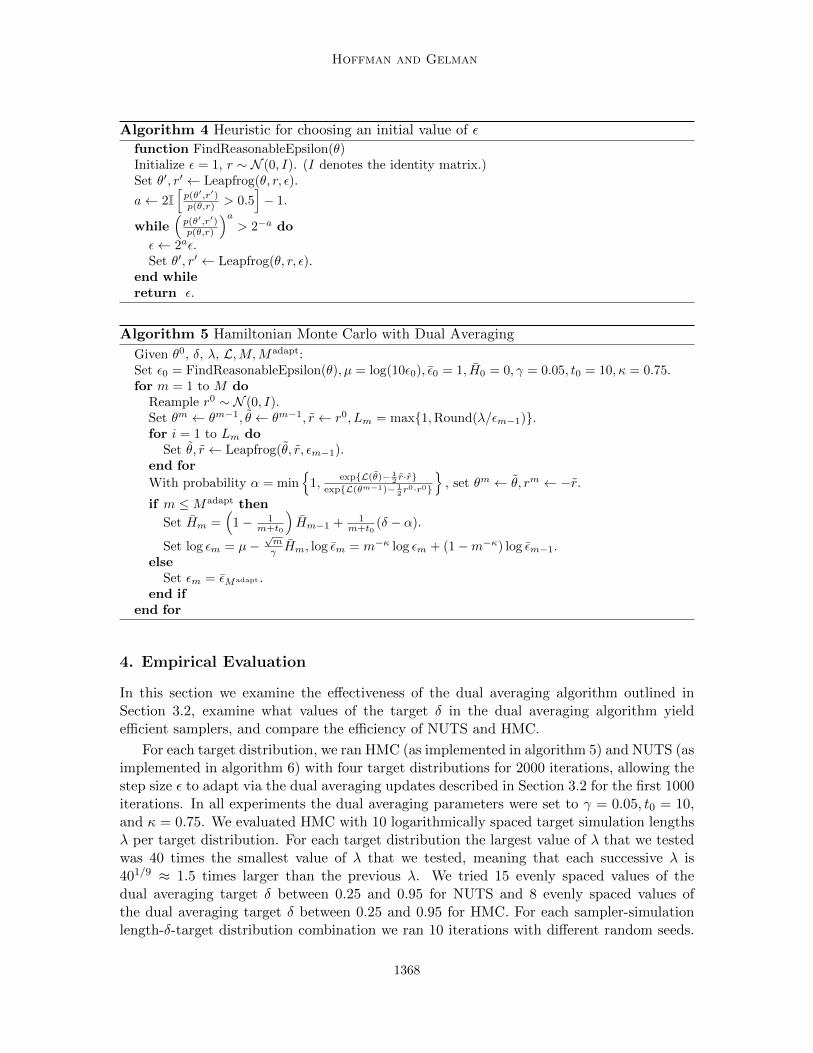
Algorithms 5 and 6 show how to implement HMC (with simulation length specified interms of εL rather than L) and NUTS while incorporating the dual averaging algorithmderived in this section, with the above initialization scheme. Algorithm 5 requires as inputa target simulation length λ ≈ εL, a target mean acceptance probability δ, and a numberof iterations Madapt after which to stop the adaptation. Algorithm 6 requires only a targetmean acceptance probability δ and a number of iterations Madapt.

1367

Hoffman and Gelman

Algorithm 4 Heuristic for choosing an initial value of ε

function FindReasonableEpsilon(θ)Initialize ε = 1, r ∼ N (0, I). (I denotes the identity matrix.)Set θ′, r′ ← Leapfrog(θ, r, ε).

a← 2I[p(θ′,r′)p(θ,r) > 0.5

]− 1.

while(p(θ′,r′)p(θ,r)

)a> 2−a do

ε← 2aε.Set θ′, r′ ← Leapfrog(θ, r, ε).

end whilereturn ε.

Algorithm 5 Hamiltonian Monte Carlo with Dual Averaging

Given θ0, δ, λ, L,M,Madapt:Set ε0 = FindReasonableEpsilon(θ), µ = log(10ε0), ε0 = 1, H0 = 0, γ = 0.05, t0 = 10, κ = 0.75.for m = 1 to M do

Reample r0 ∼ N (0, I).Set θm ← θm−1, θ ← θm−1, r ← r0, Lm = max{1,Round(λ/εm−1)}.for i = 1 to Lm do

Set θ, r ← Leapfrog(θ, r, εm−1).end for

With probability α = min{

1,exp{L(θ)− 1

2 r·r}exp{L(θm−1)− 1

2 r0·r0}

}, set θm ← θ, rm ← −r.

if m ≤Madapt then

Set Hm =(

1− 1m+t0

)Hm−1 + 1

m+t0(δ − α).

Set log εm = µ−√mγ Hm, log εm = m−κ log εm + (1−m−κ) log εm−1.

elseSet εm = εMadapt .

end ifend for

4. Empirical Evaluation

In this section we examine the effectiveness of the dual averaging algorithm outlined inSection 3.2, examine what values of the target δ in the dual averaging algorithm yieldefficient samplers, and compare the efficiency of NUTS and HMC.

For each target distribution, we ran HMC (as implemented in algorithm 5) and NUTS (asimplemented in algorithm 6) with four target distributions for 2000 iterations, allowing thestep size ε to adapt via the dual averaging updates described in Section 3.2 for the first 1000iterations. In all experiments the dual averaging parameters were set to γ = 0.05, t0 = 10,and κ = 0.75. We evaluated HMC with 10 logarithmically spaced target simulation lengthsλ per target distribution. For each target distribution the largest value of λ that we testedwas 40 times the smallest value of λ that we tested, meaning that each successive λ is401/9 ≈ 1.5 times larger than the previous λ. We tried 15 evenly spaced values of thedual averaging target δ between 0.25 and 0.95 for NUTS and 8 evenly spaced values ofthe dual averaging target δ between 0.25 and 0.95 for HMC. For each sampler-simulationlength-δ-target distribution combination we ran 10 iterations with different random seeds.

1368


Algorithm 6 No-U-Turn Sampler with Dual Averaging

Given θ0, δ, L,M,Madapt:Set ε0 = FindReasonableEpsilon(θ), µ = log(10ε0), ε0 = 1, H0 = 0, γ = 0.05, t0 = 10, κ = 0.75.for m = 1 to M do

Sample r0 ∼ N (0, I).Resample u ∼ Uniform([0, exp{L(θm−1 − 1

2r0 · r0}])

Initialize θ− = θm−1, θ+ = θm−1, r− = r0, r+ = r0, j = 0, θm = θm−1, n = 1, s = 1.while s = 1 do

Choose a direction vj ∼ Uniform({−1, 1}).if vj = −1 thenθ−, r−,−,−, θ′, n′, s′, α, nα ← BuildTree(θ−, r−, u, vj , j, εm−1θ

m−1, r0).else−,−, θ+, r+, θ′, n′, s′, α, nα ← BuildTree(θ+, r+, u, vj , j, εm−1, θ

m−1, r0).end ifif s′ = 1 then

With probability min{1, n′

n}, set θm ← θ′.

end ifn← n+ n′.s← s′I[(θ+ − θ−) · r− ≥ 0]I[(θ+ − θ−) · r+ ≥ 0].j ← j + 1.

end whileif m ≤Madapt then

Set Hm =(

1− 1m+t0

)Hm−1 + 1

m+t0(δ − α

nα).

Set log εm = µ−√mγHm, log εm = m−κ log εm + (1−m−κ) log εm−1.

elseSet εm = εMadapt .

end ifend for

function BuildTree(θ, r, u, v, j, ε, θ0, r0)if j = 0 then

Base case—take one leapfrog step in the direction v.θ′, r′ ← Leapfrog(θ, r, vε).n′ ← I[u ≤ exp{L(θ′)− 1

2r′ · r′}].

s′ ← I[u < exp{∆max + L(θ′)− 12r′ · r′}].

return θ′, r′, θ′, r′, θ′, n′, s′,min{1, exp{L(θ′)− 12r′ · r′ − L(θ0) + 1

2r0 · r0}}, 1.

elseRecursion—implicitly build the left and right subtrees.θ−, r−, θ+, r+, θ′, n′, s′, α′, n′α ← BuildTree(θ, r, u, v, j − 1, ε, θ0, r0).if s′ = 1 then

if v = −1 thenθ−, r−,−,−, θ′′, n′′, s′′, α′′, n′′α ← BuildTree(θ−, r−, u, v, j − 1, ε, θ0, r0).

else−,−, θ+, r+, θ′′, n′′, s′′, α′′, n′′α ← BuildTree(θ+, r+, u, v, j − 1, ε, θ0, r0).

end ifWith probability n′′

n′+n′′ , set θ′ ← θ′′.

Set α′ ← α′ + α′′, n′α ← n′α + n′′α.s′ ← s′′I[(θ+ − θ−) · r− ≥ 0]I[(θ+ − θ−) · r+ ≥ 0]n′ ← n′ + n′′

end ifreturn θ−, r−, θ+, r+, θ′, n′, s′, α′, n′α.

end if

1369

Hoffman and Gelman

In total, we ran 3,200 experiments with HMC and 600 experiments with NUTS. TraditionalHMC can sometimes exhibit pathological behavior when using a fixed step size and numberof steps per iteration (Neal, 2011), so after warmup we jitter HMC’s step size, samplingit uniformly at random each iteration from the range [0.9εMadapt , 1.1εMadapt ] so that thetrajectory length may vary by ±10% each iteration.

We measure the efficiency of each algorithm in terms of effective sample size (ESS)normalized by the number of gradient evaluations used by each algorithm. The ESS ofa set of M correlated samples θ1:M with respect to some function f(θ) is the number ofindependent draws from the target distribution p(θ) that would give a Monte Carlo estimateof the mean under p of f(θ) with the same level of precision as the estimate given by themean of f for the correlated samples θ1:M . That is, the ESS of a sample is a measureof how many independent samples a set of correlated samples is worth for the purposes ofestimating the mean of some function; a more efficient sampler will give a larger ESS for lesscomputation. We use the number of gradient evaluations performed by an algorithm as aproxy for the total amount of computation performed; in all of the models and distributionswe tested the computational overhead of both HMC and NUTS is dominated by the costof computing gradients. Details of the method we use to estimate ESS are provided inappendix A. In each experiment, we discarded the first 1000 samples as warmup whenestimating ESS.

ESS is inherently a univariate statistic, but all of the distributions we test HMC andNUTS on are multivariate. Following Girolami and Calderhead (2011) we compute ESSseparately for each dimension and report the minimum ESS across all dimensions, since wewant our samplers to effectively explore all dimensions of the target distribution. For eachdimension we compute ESS in terms of the variance of the estimator of that dimension’smean and second central moment (where the estimate of the mean used to compute thesecond central moment is taken from a separate long run of 50,000 iterations of NUTS withδ = 0.5), reporting whichever statistic has a lower effective sample size. We include thesecond central moment as well as the mean in order to measure each algorithm’s ability toestimate uncertainty.

4.1 Models and Data Sets

To evaluate NUTS and HMC, we used the two algorithms to sample from four target distri-butions, one of which was synthetic and the other three of which are posterior distributionsarising from real data sets.

4.1.1 250-dimensional Multivariate Normal (MVN)

In these experiments the target distribution was a zero-mean 250-dimensional multivariatenormal with known precision matrix A, that is,

p(θ) ∝ exp{−12θTAθ}.

The matrix A was generated from a Wishart distribution with identity scale matrix and250 degrees of freedom. This yields a target distribution with many strong correlations.The same matrix A was used in all experiments.

1370


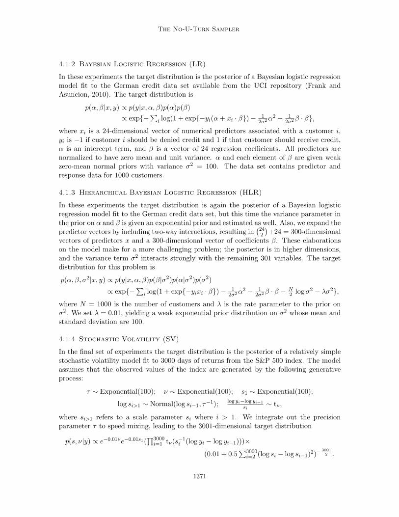
4.1.2 Bayesian Logistic Regression (LR)

In these experiments the target distribution is the posterior of a Bayesian logistic regressionmodel fit to the German credit data set available from the UCI repository (Frank andAsuncion, 2010). The target distribution is

p(α, β|x, y) ∝ p(y|x, α, β)p(α)p(β)

∝ exp{−∑

i log(1 + exp{−yi(α+ xi · β})− 12σ2α

2 − 12σ2β · β},

where xi is a 24-dimensional vector of numerical predictors associated with a customer i,yi is −1 if customer i should be denied credit and 1 if that customer should receive credit,α is an intercept term, and β is a vector of 24 regression coefficients. All predictors arenormalized to have zero mean and unit variance. α and each element of β are given weakzero-mean normal priors with variance σ2 = 100. The data set contains predictor andresponse data for 1000 customers.

4.1.3 Hierarchical Bayesian Logistic Regression (HLR)

In these experiments the target distribution is again the posterior of a Bayesian logisticregression model fit to the German credit data set, but this time the variance parameter inthe prior on α and β is given an exponential prior and estimated as well. Also, we expand thepredictor vectors by including two-way interactions, resulting in

(242

)+24 = 300-dimensional

vectors of predictors x and a 300-dimensional vector of coefficients β. These elaborationson the model make for a more challenging problem; the posterior is in higher dimensions,and the variance term σ2 interacts strongly with the remaining 301 variables. The targetdistribution for this problem is

p(α, β, σ2|x, y) ∝ p(y|x, α, β)p(β|σ2)p(α|σ2)p(σ2)

∝ exp{−∑

i log(1 + exp{−yixi · β})− 12σ2α

2 − 12σ2β · β − N

2 log σ2 − λσ2},

where N = 1000 is the number of customers and λ is the rate parameter to the prior onσ2. We set λ = 0.01, yielding a weak exponential prior distribution on σ2 whose mean andstandard deviation are 100.

4.1.4 Stochastic Volatility (SV)

In the final set of experiments the target distribution is the posterior of a relatively simplestochastic volatility model fit to 3000 days of returns from the S&P 500 index. The modelassumes that the observed values of the index are generated by the following generativeprocess:

τ ∼ Exponential(100); ν ∼ Exponential(100); s1 ∼ Exponential(100);

log si>1 ∼ Normal(log si−1, τ−1); log yi−log yi−1

si∼ tν ,

where si>1 refers to a scale parameter si where i > 1. We integrate out the precisionparameter τ to speed mixing, leading to the 3001-dimensional target distribution

p(s, ν|y) ∝ e−0.01νe−0.01s1(∏3000i=1 tν(s−1

i (log yi − log yi−1)))×

(0.01 + 0.5∑3000

i=2 (log si − log si−1)2)−3001

2 .

1371

Hoffman and Gelman

NUTS HMC εL ≈ 1.5 HMC εL ≈ 3.4 HMC εL ≈ 7.8 HMC εL ≈ 18 HMC εL ≈ 40

−0.10

0.00

0.10

0.20

0.4 0.6 0.8 0.4 0.6 0.8 0.4 0.6 0.8 0.4 0.6 0.8 0.4 0.6 0.8 0.4 0.6 0.8

Target acceptance rate statistic δ

h−δ

Normal

NUTS HMC εL ≈ 0.075 HMC εL ≈ 0.17 HMC εL ≈ 0.39 HMC εL ≈ 0.88 HMC εL ≈ 2

−0.10

0.00

0.10

0.20

0.4 0.6 0.8 0.4 0.6 0.8 0.4 0.6 0.8 0.4 0.6 0.8 0.4 0.6 0.8 0.4 0.6 0.8


h−δ

Logistic Regression


−0.10

0.00

0.10

0.20

0.4 0.6 0.8 0.4 0.6 0.8 0.4 0.6 0.8 0.4 0.6 0.8 0.4 0.6 0.8 0.4 0.6 0.8


h−δ

Hierarchical Logistic Regression


−0.10

0.00

0.10

0.20

0.4 0.6 0.8 0.4 0.6 0.8 0.4 0.6 0.8 0.4 0.6 0.8 0.4 0.6 0.8 0.4 0.6 0.8


h−δ

Stochastic Volatility

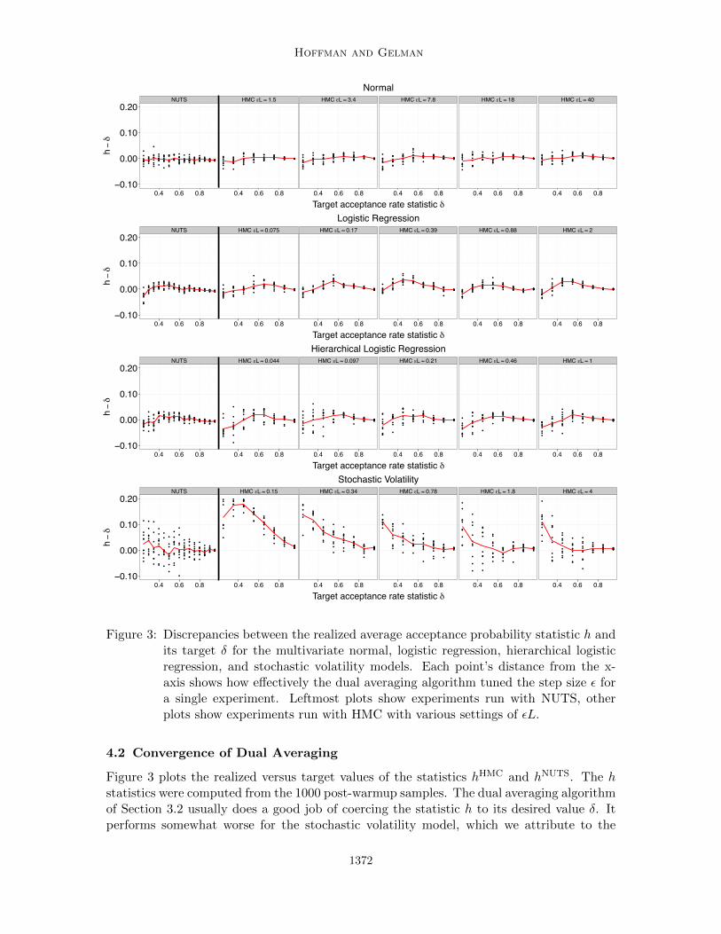
Figure 3: Discrepancies between the realized average acceptance probability statistic h andits target δ for the multivariate normal, logistic regression, hierarchical logisticregression, and stochastic volatility models. Each point’s distance from the x-axis shows how effectively the dual averaging algorithm tuned the step size ε fora single experiment. Leftmost plots show experiments run with NUTS, otherplots show experiments run with HMC with various settings of εL.

4.2 Convergence of Dual Averaging

Figure 3 plots the realized versus target values of the statistics hHMC and hNUTS. The hstatistics were computed from the 1000 post-warmup samples. The dual averaging algorithmof Section 3.2 usually does a good job of coercing the statistic h to its desired value δ. Itperforms somewhat worse for the stochastic volatility model, which we attribute to the

1372


iteration

ε / fin

al ε

0.0

0.5

1.0

1.5

2.0

MVN

0 200 400 600 800

LR

0 200 400 600 800

HLR

0 200 400 600 800

SV

0 200 400 600 800

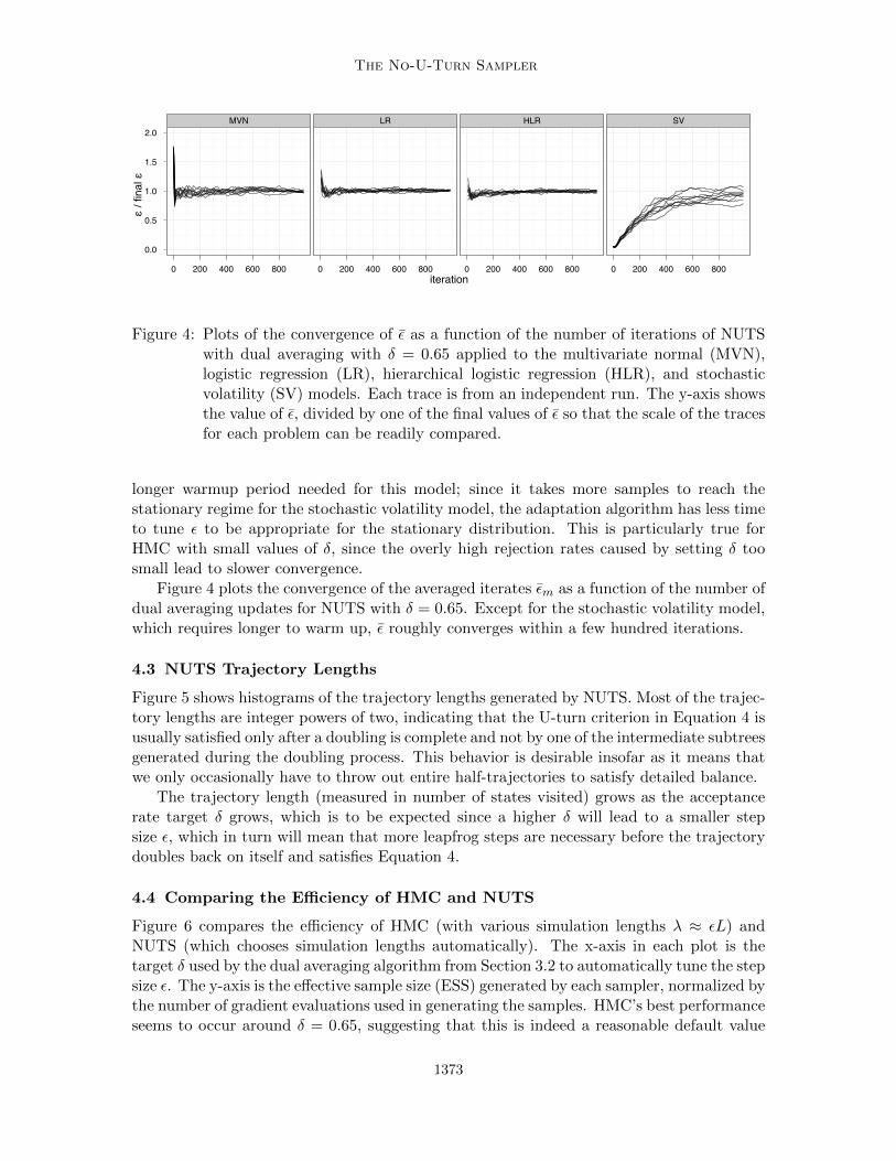
Figure 4: Plots of the convergence of ε as a function of the number of iterations of NUTSwith dual averaging with δ = 0.65 applied to the multivariate normal (MVN),logistic regression (LR), hierarchical logistic regression (HLR), and stochasticvolatility (SV) models. Each trace is from an independent run. The y-axis showsthe value of ε, divided by one of the final values of ε so that the scale of the tracesfor each problem can be readily compared.

longer warmup period needed for this model; since it takes more samples to reach thestationary regime for the stochastic volatility model, the adaptation algorithm has less timeto tune ε to be appropriate for the stationary distribution. This is particularly true forHMC with small values of δ, since the overly high rejection rates caused by setting δ toosmall lead to slower convergence.

Figure 4 plots the convergence of the averaged iterates εm as a function of the number ofdual averaging updates for NUTS with δ = 0.65. Except for the stochastic volatility model,which requires longer to warm up, ε roughly converges within a few hundred iterations.

4.3 NUTS Trajectory Lengths

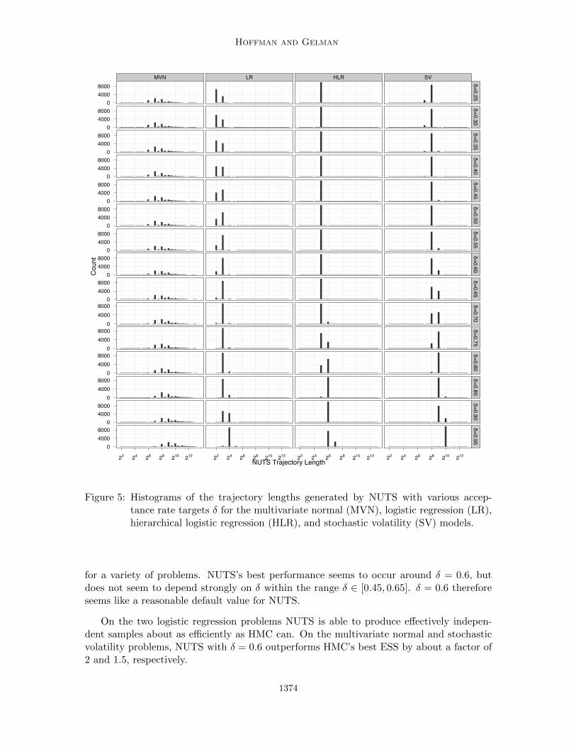
Figure 5 shows histograms of the trajectory lengths generated by NUTS. Most of the trajec-tory lengths are integer powers of two, indicating that the U-turn criterion in Equation 4 isusually satisfied only after a doubling is complete and not by one of the intermediate subtreesgenerated during the doubling process. This behavior is desirable insofar as it means thatwe only occasionally have to throw out entire half-trajectories to satisfy detailed balance.

The trajectory length (measured in number of states visited) grows as the acceptancerate target δ grows, which is to be expected since a higher δ will lead to a smaller stepsize ε, which in turn will mean that more leapfrog steps are necessary before the trajectorydoubles back on itself and satisfies Equation 4.

4.4 Comparing the Efficiency of HMC and NUTS

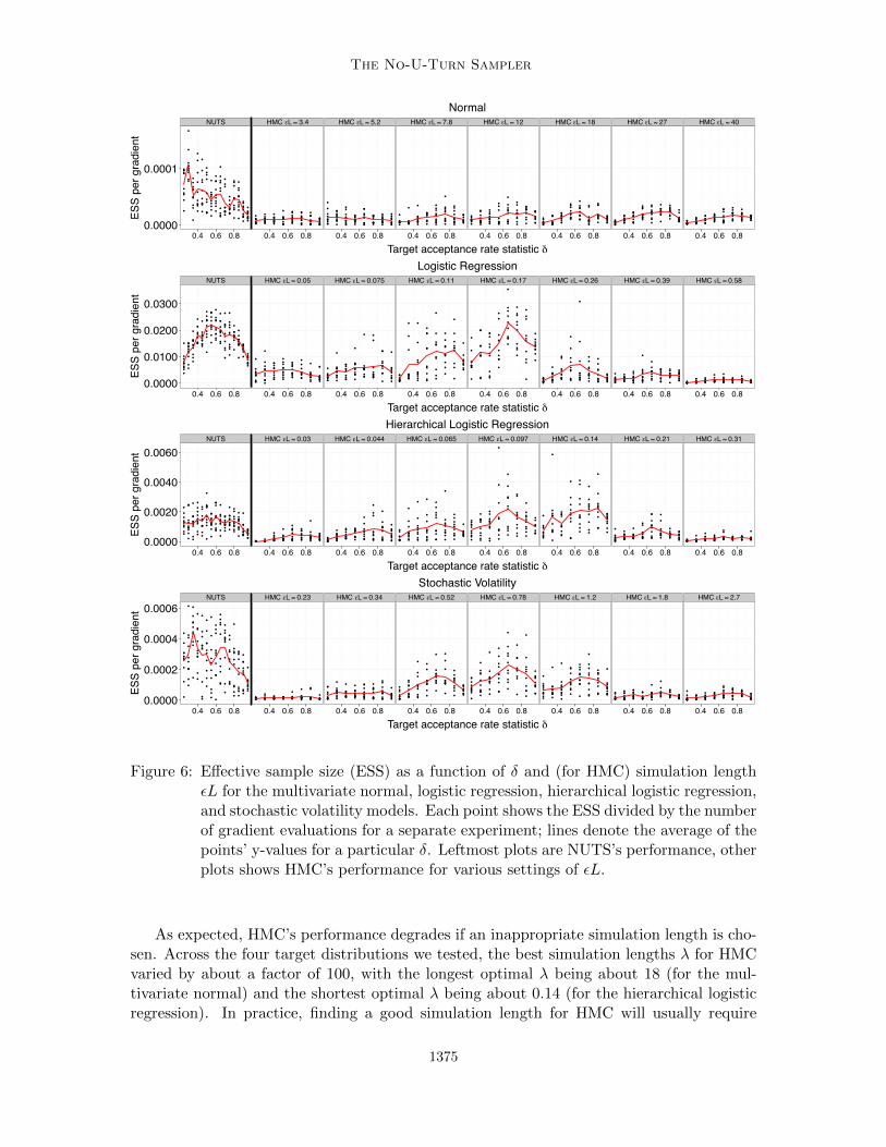
Figure 6 compares the efficiency of HMC (with various simulation lengths λ ≈ εL) andNUTS (which chooses simulation lengths automatically). The x-axis in each plot is thetarget δ used by the dual averaging algorithm from Section 3.2 to automatically tune the stepsize ε. The y-axis is the effective sample size (ESS) generated by each sampler, normalized bythe number of gradient evaluations used in generating the samples. HMC’s best performanceseems to occur around δ = 0.65, suggesting that this is indeed a reasonable default value

1373

Hoffman and Gelman

NUTS Trajectory Length

Co

un

t

0

4000

8000

0

4000

8000

0

4000

8000

0

4000

8000

0

4000

8000

0

4000

8000

0

4000

8000

0

4000

8000

0

4000

8000

0

4000

8000

0

4000

8000

0

4000

8000

0

4000

8000

0

4000

8000

0

4000

8000

MVN

22 24 26 28 210 212

LR

22 24 26 28 210 212

HLR

22 24 26 28 210 212

SV

22 24 26 28 210 212

δ=

0.2

5δ

=0

.30

δ=

0.3

5δ

=0

.40

δ=

0.4

5δ

=0

.50

δ=

0.5

5δ

=0

.60

δ=

0.6

5δ

=0

.70

δ=

0.7

5δ

=0

.80

δ=

0.8

5δ

=0

.90

δ=

0.9

5

Figure 5: Histograms of the trajectory lengths generated by NUTS with various accep-tance rate targets δ for the multivariate normal (MVN), logistic regression (LR),hierarchical logistic regression (HLR), and stochastic volatility (SV) models.

for a variety of problems. NUTS’s best performance seems to occur around δ = 0.6, butdoes not seem to depend strongly on δ within the range δ ∈ [0.45, 0.65]. δ = 0.6 thereforeseems like a reasonable default value for NUTS.

On the two logistic regression problems NUTS is able to produce effectively indepen-dent samples about as efficiently as HMC can. On the multivariate normal and stochasticvolatility problems, NUTS with δ = 0.6 outperforms HMC’s best ESS by about a factor of2 and 1.5, respectively.

1374


NUTS HMC εL ≈ 3.4 HMC εL ≈ 5.2 HMC εL ≈ 7.8 HMC εL ≈ 12 HMC εL ≈ 18 HMC εL ≈ 27 HMC εL ≈ 40

0.0000

0.0001

0.4 0.6 0.8 0.4 0.6 0.8 0.4 0.6 0.8 0.4 0.6 0.8 0.4 0.6 0.8 0.4 0.6 0.8 0.4 0.6 0.8 0.4 0.6 0.8


ESS

per g

radi

ent

Normal

NUTS HMC εL ≈ 0.05 HMC εL ≈ 0.075 HMC εL ≈ 0.11 HMC εL ≈ 0.17 HMC εL ≈ 0.26 HMC εL ≈ 0.39 HMC εL ≈ 0.58

0.0000

0.0100

0.0200

0.0300

0.4 0.6 0.8 0.4 0.6 0.8 0.4 0.6 0.8 0.4 0.6 0.8 0.4 0.6 0.8 0.4 0.6 0.8 0.4 0.6 0.8 0.4 0.6 0.8


ESS

per g

radi

ent

Logistic Regression


0.0000

0.0020

0.0040

0.0060

0.4 0.6 0.8 0.4 0.6 0.8 0.4 0.6 0.8 0.4 0.6 0.8 0.4 0.6 0.8 0.4 0.6 0.8 0.4 0.6 0.8 0.4 0.6 0.8


ESS

per g

radi

ent

Hierarchical Logistic Regression


0.0000

0.0002

0.0004

0.0006

0.4 0.6 0.8 0.4 0.6 0.8 0.4 0.6 0.8 0.4 0.6 0.8 0.4 0.6 0.8 0.4 0.6 0.8 0.4 0.6 0.8 0.4 0.6 0.8


ESS

per g

radi

ent

Stochastic Volatility

Figure 6: Effective sample size (ESS) as a function of δ and (for HMC) simulation lengthεL for the multivariate normal, logistic regression, hierarchical logistic regression,and stochastic volatility models. Each point shows the ESS divided by the numberof gradient evaluations for a separate experiment; lines denote the average of thepoints’ y-values for a particular δ. Leftmost plots are NUTS’s performance, otherplots shows HMC’s performance for various settings of εL.

As expected, HMC’s performance degrades if an inappropriate simulation length is cho-sen. Across the four target distributions we tested, the best simulation lengths λ for HMCvaried by about a factor of 100, with the longest optimal λ being about 18 (for the mul-tivariate normal) and the shortest optimal λ being about 0.14 (for the hierarchical logisticregression). In practice, finding a good simulation length for HMC will usually require

1375

Hoffman and Gelman

-3

-2

-1

0

1

2

3

Metropolis

-15 -10 -5 0 5 10 15

Gibbs

-15 -10 -5 0 5 10 15

NUTS

-15 -10 -5 0 5 10 15

Independent

-15 -10 -5 0 5 10 15

Figure 7: Samples generated by random-walk Metropolis, Gibbs sampling, and NUTS. Theplots compare 1,000 independent draws from a highly correlated 250-dimensionaldistribution (right) with 1,000,000 samples (thinned to 1,000 samples for display)generated by random-walk Metropolis (left), 1,000,000 samples (thinned to 1,000samples for display) generated by Gibbs sampling (second from left), and 1,000samples generated by NUTS (second from right). Only the first two dimensionsare shown here.

some number of preliminary runs. The results in Figure 6 suggest that NUTS can generatesamples at least as efficiently as HMC, even discounting the cost of any preliminary runsneeded to tune HMC’s simulation length.

4.5 Qualitative Comparison of NUTS, Random-Walk Metropolis, and Gibbs

In Section 4.4, we compared the efficiency of NUTS and HMC. In this section, we informallydemonstrate the advantages of NUTS over the popular random-walk Metropolis (RWM)and Gibbs sampling algorithms. We ran NUTS, RWM, and Gibbs sampling on the 250-dimensional multivariate normal distribution described in Section 4.1. NUTS was run withδ = 0.5 for 2,000 iterations, with the first 1,000 iterations being used as warmup and toadapt ε. This required about 1,000,000 gradient and likelihood evaluations in total. Weran RWM for 1,000,000 iterations with an isotropic normal proposal distribution whosevariance was selected beforehand to produce the theoretically optimal acceptance rate of0.234 (Gelman et al., 1996). The cost per iteration of RWM is effectively identical to the costper gradient evaluation of NUTS, and the two algorithms ran for about the same amountof time. We ran Gibbs sampling for 1,000,000 sweeps over the 250 parameters. This tooklonger to run than NUTS and RWM, since for the multivariate normal each Gibbs sweepcosts more than a single gradient evaluation; we chose to nonetheless run the same numberof Gibbs sweeps as RWM iterations, since for some other models Gibbs sweeps can be donemore efficiently.

Figure 7 visually compares independent samples (projected onto the first two dimen-sions) from the target distribution with samples generated by the three MCMC algorithms.RWM has barely begun to explore the space. Gibbs does better, but still has left parts

1376


of the space unexplored. NUTS, on the other hand, is able to generate many effectivelyindependent samples.

We use this simple example to visualize the relative performance of NUTS, Gibbs,and RWM on a moderately high-dimensional distribution exhibiting strong correlations.For the multivariate normal, Gibbs or RWM would of course work much better after anappropriate rotation of the parameter space. But finding and applying an appropriaterotation can be expensive when the number of parameters D gets large, and RWM andGibbs both require O(D2) operations per effectively independent sample even under thehighly optimistic assumption that a transformation can be found that renders all parametersi.i.d. and can be applied cheaply (e.g., in O(D) rather than the usual O(D2) cost of matrix-vector multiplication and the O(D3) cost of matrix inversion). This is shown for RWM byCreutz (1988), and for Gibbs is the result of needing to apply a transformation requiringO(D) operations D times per Gibbs sweep. For complicated models, even more expensivetransformations often cannot render the parameters sufficiently independent to make RWMand Gibbs run efficiently. NUTS, on the other hand, is able to efficiently sample fromhigh-dimensional target distributions without needing to be tuned to the shape of thosedistributions.

5. Discussion

We have presented the No-U-Turn Sampler (NUTS), a variant of the powerful Hamilto-nian Monte Carlo (HMC) Markov chain Monte Carlo (MCMC) algorithm that eliminatesHMC’s dependence on a number-of-steps parameter L but retains (and in some cases im-proves upon) HMC’s ability to generate effectively independent samples efficiently. We alsodeveloped a method for automatically adapting the step size parameter ε shared by NUTSand HMC via an adaptation of the dual averaging algorithm of Nesterov (2009), makingit possible to run NUTS with no hand tuning at all. The dual averaging approach wedeveloped in this paper could also be applied to other MCMC algorithms in place of moretraditional adaptive MCMC approaches based on the Robbins-Monro stochastic approxi-mation algorithm (Andrieu and Thoms, 2008; Robbins and Monro, 1951).

In this paper we have only compared NUTS with the basic HMC algorithm, and notits extensions, several of which are reviewed by Neal (2011). We only considered simplekinetic energy functions of the form 1

2r · r, but both NUTS and HMC can benefit fromintroducing a “mass” matrix M and using the kinetic energy function 1

2rTM−1r. If M−1

approximates the covariance matrix of p(θ), then this kinetic energy function will reduce thenegative impacts strong correlations and bad scaling have on the efficiency of both NUTSand HMC; indeed, experiments with hierarchical regression models with high correlationsshow substantial reduction in total computation time from nonidentity and nondiagonalmass matrices. Fitting an appropriate mass matrix can only be done during the warmupstage, and care must be taken to ensure the stability of the fitting procedure. Since usinga mass matrix is equivalent to linearly transforming the parameter space (Neal, 2011), theno-U-turn condition should be computed on the transformed parameters instead of in theoriginal space.

Another extension of HMC introduced by Neal (1994) considers windows of proposedstates rather than simply the state at the end of the trajectory to allow for larger step sizes

1377

Hoffman and Gelman

without sacrificing acceptance rates (at the expense of introducing a window size parameterthat must be tuned). The effectiveness of the windowed HMC algorithm suggests thatNUTS’s lack of a single accept/reject step may be responsible for some of its performancegains over vanilla HMC.

Girolami and Calderhead (2011) recently introduced Riemannian Manifold Hamilto-nian Monte Carlo (RMHMC), a variant on HMC that simulates Hamiltonian dynamics inRiemannian rather than Euclidean spaces, effectively allowing for position-dependent massmatrices. Although the worst-case O(D3) matrix inversion costs associated with this al-gorithm often make it expensive to apply in high dimensions, when these costs are nottoo onerous RMHMC’s ability to adapt its kinetic energy function makes it very efficient.There are no technical barriers that stand in the way of combining NUTS’s ability to adaptits trajectory lengths with RMHMC’s ability to adapt its mass matrices, although naivelyapplying the no-U-turn condition (which is tied to Euclidean geometry) to Riemannianalgorithms may be suboptimal (Betancourt, 2013).

Like HMC, NUTS can only be used to resample unconstrained continuous-valued vari-ables with respect to which the target distribution is differentiable almost everywhere. HMCand NUTS can deal with simple constraints such as nonnegativity or restriction to the sim-plex by an appropriate change of variable, but discrete variables must either be summed outor handled by other algorithms such as Gibbs sampling. In models with discrete variables,NUTS’s ability to automatically choose a trajectory length may make it more effective thanHMC when discrete variables are present, since it is not tied to a single simulation lengththat may be appropriate for one setting of the discrete variables but not for others.

Some models include hard constraints that are too complex to eliminate by a simplechange of variables. Such models will have regions of the parameter space with zero posteriorprobability. When HMC encounters such a region, the best it can do is stop short and restartwith a new momentum vector, wasting any work done before violating the constraints (Neal,2011). By contrast, when NUTS encounters a zero-probability region it stops short andsamples from the set of points visited up to that point, making at least some progress.

NUTS with dual averaging makes it possible for Bayesian data analysts to obtain theefficiency of HMC without spending time and effort hand-tuning HMC’s parameters. Thisis desirable even for those practitioners who have experience using and tuning HMC, but itis especially valuable for those who lack this experience. In particular, NUTS’s ability tooperate efficiently without user intervention makes it well suited for use in generic inferenceengines in the mold of BUGS (Gilks and Spiegelhalter, 1992), which until now have largelyrelied on much less efficient algorithms such as Gibbs sampling. We are currently developingan automatic Bayesian inference system called Stan, which uses NUTS as its core inferencealgorithm for continuous-valued parameters (Stan Development Team, 2013). Stan promisesto be able to generate effectively independent samples from complex models’ posteriorsorders of magnitude faster than previous systems such as BUGS and JAGS (Plummer,2003).

In summary, NUTS makes it possible to efficiently perform Bayesian posterior inferenceon a large class of complex, high-dimensional models with minimal human intervention. It isour hope that NUTS will allow researchers and data analysts to spend more time developingand testing models and less time worrying about how to fit those models to data.

1378


Acknowledgments

We thank Bob Carpenter, Michael Betancourt, and Radford Neal for helpful comments.This work was partially supported by Institute of Education Sciences grant ED-GRANTS-032309-005, Department of Energy grant DE-SC0002099, National Science Foundationgrant ATM-0934516, and National Science Foundation grant SES-1023189.

Appendix A. Estimating Effective Sample Size

For a function f(θ), a target distribution p(θ), and a Markov chain Monte Carlo (MCMC)sampler that produces a set of M correlated samples drawn from some distribution q(θ1:M )such that q(θm) = p(θm) for any m ∈ {1, . . . ,M}, the effective sample size (ESS) of θ1:M isthe number of independent samples that would be needed to obtain a Monte Carlo estimateof the mean of f with equal variance to the MCMC estimate of the mean of f :

ESSq,f (θ1:M ) = MVq[ 1

M

∑Ms=1 f(θs)]

Vp[f(θ)]M

=M

1 + 2∑M−1

s=1 (1− sM )ρfs

;

ρfs ≡Eq[(f(θt)− Ep[f(θ)])(f(θt−s)− Ep[f(θ)])]

Vp[f(θ)],

where ρfs denotes the autocorrelation under q of f at lag s and Vp[x] denotes the varianceof a random variable x under the distribution p(x).

To estimate ESS, we first compute the following estimate of the autocorrelation spectrumfor the function f(θ):

ρfs =1

σ2f (M − s)

M∑m=s+1

(f(θm)− µf )(f(θm−s)− µf ),

where the estimates µf and σ2f of the mean and variance of the function f are computed with

high precision from a separated 50,000-sample run of NUTS with δ = 0.5. We do not takethese estimates from the chain whose autocorrelations we are trying to estimate—doingso can lead to serious underestimates of the level of autocorrelation (and thus a seriousoverestimate of the number of effective samples) if the chain has not yet converged or hasnot yet generated a fair number of effectively independent samples.

Any estimator of ρfs is necessarily noisy for large lags s, so using the naive estimatorˆESSq,f (θ1:M ) = M

1+2∑M−1s=1 (1− s

M)ρfs

will yield bad results. Instead, we truncate the sum over

the autocorrelations when the autocorrelations first dip below 0.05, yielding the estimator

ˆESSq,f (θ1:M ) =M

1 + 2∑Mcutoff

f

s=1 (1− sM )ρfs

; M cutofff ≡ min

ss s.t. ρfs < 0.05.

We found that this method for estimating ESS gave more reliable confidence intervalsfor MCMC estimators than the autoregressive approach used by CODA (Plummer et al.,2006). (The more accurate estimator comes at the expense of needing to compute a costlyhigh-quality estimate of the true mean and variance of the target distribution.) The 0.05cutoff is somewhat arbitrary; in our experiments we did not find the results to be verysensitive to the precise value of this cutoff.

1379

Hoffman and Gelman

References

C. Andrieu and J. Thoms. A tutorial on adaptive MCMC. Statistics and Computing, 18(4):343–373, 2008.

A. Beskos, N. Pillai, G. Roberts, J. Sanz-Serna, and A. Stuart. Optimal tuning of thehybrid monte-carlo algorithm. Arxiv preprint arXiv:1001.4460, 2010.

M. Betancourt. Generalizing the no-U-turn sampler to Riemannian manifolds. ArXivpreprint arXiv:1304.1920, 2013.

M. Creutz. Global Monte Carlo algorithms for many-fermion systems. Physical Review D,38(4):1228–1238, 1988.

H. Daume III. HBC: Hierarchical Bayes compiler, 2007. URL http://hal3.name/HBC.

A. Duane, A. Kennedy, B. Pendleton, and D. Roweth. Hybrid Monte Carlo. Physics LettersB, 195(2):216–222, 1987.

A. Frank and A. Asuncion. UCI machine learning repository, 2010. URL http://archive.

ics.uci.edu/ml.

A. Gelman, G. Roberts, and W. Gilks. Efficient Metropolis jumping rules. Bayesian Statis-tics, 5:599–608, 1996.

A. Gelman, J. Carlin, H. Stern, and D. Rubin. Bayesian Data Analysis. Chapman & Hall,2004.

S. Geman and D. Geman. Stochastic relaxation, Gibbs distributions and the Bayesianrestoration of images. IEEE Transactions on Pattern Analysis and Machine Intelligence,6:721–741, 1984.

W. Gilks and D. Spiegelhalter. A language and program for complex Bayesian modelling.The Statistician, 3:169–177, 1992.

M. Girolami and B. Calderhead. Riemann manifold Langevin and Hamiltonian Monte Carlomethods. Journal of the Royal Statistical Society: Series B (Statistical Methodology), 73(2):123–214, 2011.

A. Griewank and A. Walther. Evaluating Derivatives: Principles and Techniques of Algo-rithmic Differentiation. Society for Industrial and Applied Mathematics (SIAM), 2008.

S. Lan, V. Stathopoulos, B. Shahbaba, and M. Girolami. Lagrangian Dynamical MonteCarlo. ArXiv preprint arXiv:1211.3759, 2012.

B. Leimkuhler and S. Reich. Simulating Hamiltonian Dynamics, volume 14. CambridgeUniversity Press, 2004.

N. Metropolis, A. Rosenbluth, M. Rosenbluth, M. Teller, and E. Teller. Equations of statecalculations by fast computing machines. Journal of Chemical Physics, 21:1087–1092,1953.

1380

http://hal3.name/HBC

http://archive.ics.uci.edu/ml

http://archive.ics.uci.edu/ml


T. Minka, J. Winn, J. Guiver, and D. Knowles. Infer.NET 2.4, Microsoft Research Cam-bridge, 2010., utl=http://research.microsoft.com/infernet.

R. Neal. Probabilistic inference using Markov chain Monte Carlo methods. Technical ReportCRG-TR-93-1, Department of Computer Science, University of Toronto, 1993.

R. Neal. An improved acceptance procedure for the hybrid Monte Carlo algorithm. Journalof Computational Physics, 111:194–203, 1994.

R. Neal. Slice sampling. Annals of Statistics, 31(3):705–741, 2003.

R. Neal. Handbook of Markov Chain Monte Carlo, chapter 5: MCMC Using HamiltonianDynamics. CRC Press, 2011.

Y. Nesterov. Primal-dual subgradient methods for convex problems. Mathematical Pro-gramming, 120(1):221–259, 2009.

A. Patil, D. Huard, and C. Fonnesbeck. PyMC: Bayesian stochastic modelling in python.Journal of Statistical Software, 35(4):1–81, 2010.

M. Plummer. JAGS: A program for analysis of Bayesian graphical models using Gibbssampling, 2003. URL http://sourceforge.net/projects/mcmc-jags/.

M. Plummer, N. Best, K. Cowles, and K. Vines. CODA: Convergence diagnosis and outputanalysis for MCMC. R News, 6(1):7–11, March 2006.

H. Robbins and S. Monro. A stochastic approximation method. The Annals of MathematicalStatistics, pages 400–407, 1951.

Stan Development Team. Stan: A C++ library for probability and sampling, version 1.1,2013. URL http://mc-stan.org/.

L. Tierney and A. Mira. Some adaptive Monte Carlo methods for Bayesian inference.Statistics in Medicine, 18:2507–2515, 1999.

M. Wainwright and M. Jordan. Graphical models, exponential families, and variationalinference. Foundations and Trends in Machine Learning, 1(1-2):1–305, 2008.

1381

http://sourceforge.net/projects/mcmc-jags/

http://mc-stan.org/

the no-u-turn sampler: adaptively setting path lengths in

Documents