the non-linear energy sink applied to vertical floor
TRANSCRIPT
Masthead LogoUniversity of Tennessee, KnoxvilleTrace: Tennessee Research and Creative Exchange
Masters Theses Graduate School
12-2018
The Non-Linear Energy Sink Applied to VerticalFloor Vibration MitigationJames Ridge RamseyUniversity of Tennessee, [email protected]
This Thesis is brought to you for free and open access by the Graduate School at Trace: Tennessee Research and Creative Exchange. It has beenaccepted for inclusion in Masters Theses by an authorized administrator of Trace: Tennessee Research and Creative Exchange. For more information,please contact [email protected].
Recommended CitationRamsey, James Ridge, "The Non-Linear Energy Sink Applied to Vertical Floor Vibration Mitigation. " Master's Thesis, University ofTennessee, 2018.https://trace.tennessee.edu/utk_gradthes/5381

To the Graduate Council:
I am submitting herewith a thesis written by James Ridge Ramsey entitled "The Non-Linear Energy SinkApplied to Vertical Floor Vibration Mitigation." I have examined the final electronic copy of this thesisfor form and content and recommend that it be accepted in partial fulfillment of the requirements for thedegree of Master of Science, with a major in Civil Engineering.
Nicholas Wierschem, Major Professor
We have read this thesis and recommend its acceptance:
Mark D. Denavit, Timothy J. Truster
Accepted for the Council:Carolyn R. Hodges
Vice Provost and Dean of the Graduate School
(Original signatures are on file with official student records.)

The Non-Linear Energy Sink Applied to
Vertical Floor Vibration Mitigation
A Thesis Presented for the
Master of Science
Degree
The University of Tennessee, Knoxville
James Ridge Ramsey
December 2018

ii
Abstract
This thesis investigates the non-linear energy sink (NES) and its application to floor vibration
mitigation. The NES is a passive type mass damper comprised of an essentially non-linear
stiffness component. This non-linear stiffness property allows the NES to interact with a wide
variety of frequency regimes that can vary both widely and randomly throughout flooring
systems. Flooring systems are regularly subjected to these changing inputs from general use and
occupancy, as well as, human and mechanical induced loading. It is known that the NES has
been successfully implemented for vibration mitigation in the horizontal direction. However, to
achieve this non-linearity in the vertical direction, the offset produced by gravitational force
needs to be considered. This thesis proposes an NES device that compensates for this
gravitational force and investigates its interaction and application to vertical floor vibration
mitigation. The device’s geometric mechanism and its derivation are presented, as well as, the
limitations and extent of its physical properties. In addition, a simplified floor model is derived
using structural dynamic analysis techniques and is studied under three cases which include: a
control, a traditional tuned mass damper, and the new proposed device. The results support the
assumption that the device’s non-linear restoring force can be approximately modeled as a cubic
function. This approximation allows for simplification in both the model’s analysis and
optimization stages. Also, the results show that the device can be affective at mitigating vertical
vibration modes. This supports the theory that a frequency independent non-linear mechanism
can be produced for the vertical vibration mitigation needed in flooring systems.

iii
Table of Contents
1. Introduction ............................................................................................................................... 1
2. Literature Review ..................................................................................................................... 5
2.1 Floor Vibration Mitigation Motivation ............................................................................................... 5
2.2 Mitigation Techniques & Devices ...................................................................................................... 8
System Design ...................................................................................................................................... 8
Devices ................................................................................................................................................ 14
2.3 Non-Linear Energy Sink ................................................................................................................... 20
2.4 Gravity Compensation ...................................................................................................................... 26
3. Proposed Gravity Compensated NES Device (GCNES) ..................................................... 29
3.1 Proposed Device ............................................................................................................................... 30
3.2 Restoring Force Derivation ............................................................................................................... 32
3.3 Device Realization ............................................................................................................................ 35
4. Two Degree of Freedom (2DOF) Oscillator Analysis .......................................................... 41
4.1 TMD 2DOF Analysis ........................................................................................................................ 42
4.2 NES 2DOF Analysis ......................................................................................................................... 44
4.3 GCNES 2DOF Analysis ................................................................................................................... 47
5. Floor Model ............................................................................................................................. 50
5.1 Proposed Model ................................................................................................................................ 50
5.2 Assumed Modes Method .................................................................................................................. 52
5.3 Lagrange Formulation ....................................................................................................................... 57
Control Case Formulation ................................................................................................................... 58
TMD Case Formulation ...................................................................................................................... 63
NES Case Formulation........................................................................................................................ 66
GCNES Case Formulation .................................................................................................................. 68
5.4 Modal Analysis & Damping Matrix ................................................................................................. 69
Modal Analysis ................................................................................................................................... 69
Mode Shapes ....................................................................................................................................... 70
Damping Matrix .................................................................................................................................. 74
6. Optimization ............................................................................................................................ 77
7. Beam Model Vibration Mitigation ........................................................................................ 82
7.1 Control Impulse Excitation Response ............................................................................................... 82

iv
7.2 Control, TMD, and NES Case Comparisons .................................................................................... 84
TMD Optimal Response ..................................................................................................................... 84
NES Optimal Response ....................................................................................................................... 85
Parameter Response Analysis ............................................................................................................. 86
Lumped Mass Analysis ....................................................................................................................... 89
7.3 GCNES Gravity Compensation ........................................................................................................ 95
8. Realistic GCNES Design......................................................................................................... 99
9. Conclusion ............................................................................................................................. 102
References .................................................................................................................................. 105
Appendix .................................................................................................................................... 108
Maple Solution Code ............................................................................................................................ 109
Vita ............................................................................................................................................. 132

v
List of Tables
Table 1 GCNES Parameter Solution Summary Example ........................................................................... 36
Table 2 Assumed Shape Functions ............................................................................................................. 53
Table 3 Fundamental natural frequencies ................................................................................................... 70
vi
List of Figures
Figure 1 Vertical transient vibration time history example (Wiss and Parmelee 1974) ............................. 10
Figure 2 ISO peak acceleration comfort control criteria due to human activities (Ebrahimpour and Sack
2005) ........................................................................................................................................................... 11
Figure 3 footfall forces (Left) & pedestrian footfall loading (Right) (Ellingwood and Tallin 1984) ......... 11
Figure 4 Quantified heel impact forcing function (Foschi et al. 1995) ....................................................... 13
Figure 5 VEM floor composite schematic (Left) & acceleration response (Right) (Saidi et al. 2006)
.................................................................................................................................................................... 15
Figure 6 VEM & CFRP floor joist schematic (Left) & normalized deflection plot (Right) (Ebrahimpour
and Sack 2005) ............................................................................................................................................ 16
Figure 7 PTMD (Left) & TMD (Right) (Saidi et al. 2006) ......................................................................... 18
Figure 8 BTMD (Left) & TLCD (Right) (Gutierrez Soto and Adeli 2013) ................................................ 18
Figure 9 Typical response without TMD (Left) & with TMD (Right) (Setareh and Hanson 1992)........... 19
Figure 10 Passive broadband TETs schematic (Lee et al. 2008) ................................................................ 21
Figure 11 Undamped numerical frequency energy plot solution to a simple oscillator coupled to a strong
NES device (Lee et al. 2008; McFarland et al. 2005) ................................................................................. 22
Figure 12 Detailed view of relative system displacement at orbits in the frequency energy plot (Lee et al.
2008) ........................................................................................................................................................... 23
Figure 13 Railway bridge coupled with an NES schematic (Younesian et al. 2011) ................................. 24
Figure 14 NES Input Energy Absorption vs. Position (Georgiades and Vakakis 2007) ............................ 25
Figure 15 Beam model with local continuous stiffness non-linearity under static load and sinusoidal
excitation (Royston and Singh 1996) .......................................................................................................... 27
Figure 16 Levitating magnet based non-linear energy harvesting device (Mann and Sims 2009) ............. 27
Figure 17 Quasi-zero stiffness mechanism (Right) (Carrella et al. 2007) & application in mechanical
isolator schematic (left) (Kovacic et al. 2008) ............................................................................................ 28
Figure 18 Typical NES force vs. displacement interaction and effect of gravity on initial tangent stiffness
of the device ................................................................................................................................................ 29
Figure 19 Proposed NES device schematic ................................................................................................ 31
Figure 20 Free body diagram of device restoring force .............................................................................. 32
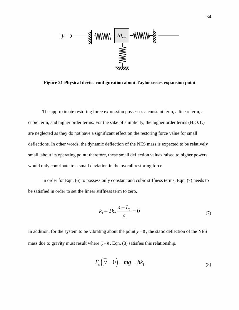
Figure 21 Physical device configuration about Taylor series expansion point ........................................... 34
Figure 22 GCNES Parametric Solution Curves .......................................................................................... 38
Figure 23 Maximum Obtainable Displacement Before 20% Restoring Force Deviation Example ........... 39
Figure 24 Percent Difference Given Displacement Limitations Example .................................................. 39
Figure 25 Restoring Forces with Multiple Horizontal Lengths Example ................................................... 40
Figure 26 2DOF Schematic Diagrams: TMD (Left), Cubic NES (Center), and GCNES (Right) .............. 42
Figure 27 TMD Impulse Time History Response without Gravity ............................................................ 43
Figure 28 TMD Impulse Time History Response with Gravity ................................................................. 44
Figure 29 NES Impulse Time History Response without Gravity .............................................................. 46
Figure 30 NES Impulse Time History Response with Gravity ................................................................... 46
Figure 31 GCNES Impulse Solution Response as Function of Horizontal Length (a) ............................... 47
Figure 32 GCNES Impulse Time History Response with Gravity ............................................................. 49
Figure 33 GCNES Impulse with Gravity Restoring Force Example .......................................................... 49

vii
Figure 34 Floor beam model coupled to a GCNES device ......................................................................... 51
Figure 35 Assumed shape functions plotted along beam length ................................................................. 56
Figure 36 Floor beam model control case diagram ..................................................................................... 58
Figure 37 Floor beam model coupled with TMD diagram ......................................................................... 63
Figure 38 Floor beam model coupled with NES diagram ........................................................................... 66
Figure 39 Modal analysis mode shapes plotted along beam length ............................................................ 73
Figure 40 TMD 2DOF Contour Optimization ............................................................................................ 78
Figure 41 NES 2DOF Contour Optimization ............................................................................................. 79
Figure 42 TMD Beam Floor Model Contour Optimization ........................................................................ 80
Figure 43 NES Beam Floor Model Contour Optimization ......................................................................... 81
Figure 44 Control Impulse Response .......................................................................................................... 83
Figure 45 Optimal Response Justification Example ................................................................................... 84
Figure 46 TMD Optimal Response ............................................................................................................. 85
Figure 47 NES Optimal Response .............................................................................................................. 86
Figure 48 Amplitude Response Comparison .............................................................................................. 87
Figure 49 Device Position Response Comparison ...................................................................................... 88
Figure 50 Load Position Response Comparison ......................................................................................... 88
Figure 51 Lumped Mass Percentage Response Comparison ...................................................................... 90
Figure 52 25% Lumped Mass Position Response Comparison .................................................................. 91
Figure 53 Load Position with 25% Lumped Mass Response Comparison ................................................. 91
Figure 54 Control 25% Lumped Mass Response ........................................................................................ 92
Figure 55 TMD 25% Lumped Mass Response ........................................................................................... 93
Figure 56 NES 25% Lumped Mass Response ............................................................................................ 94
Figure 57 Beam Response Comparison with 25% Lumped Mass .............................................................. 94
Figure 58 GCNES Parameter Response as Function of Horizontal Length ............................................... 95
Figure 59 GCNES Optimal Response ......................................................................................................... 96
Figure 60 Lumped Mass Percentage Response Comparison (Gravity Considered) ................................... 97
Figure 61 25% Lumped Mass Location Response Comparison (Gravity Considered) .............................. 98
Figure 62 25% Lumped Mass Load Position Response Comparison (Gravity Considered) ...................... 98
Figure 63 Steel-Concrete Composite Deck Girder (Wanant 2014) ............................................................ 99

viii
List of Symbols
a GCNES horizontal length
A beam cross sectional area
cTMD TMD damping coefficient
cNES NES damping coefficient
cGCNES GCNES damping coefficient
C control case damping matrix
TMDC TMD case damping matrix
NESC NES case damping matrix
C modal damping matrix
E beam modulus of Elasticity
Fd damping force
FNES NES restoring force
FGCNES GCNES relative restoring force
Fs GCNES full restoring force
Fs-approx GCNES cubic approximated restoring force
F1 GCNES inline spring force
F2 GCNES oblique spring force
g gravitational constant
h GCNES vertical length
I beam moment of inertia
mode shape matrix
kTMD TMD spring constant
kNES NES spring constant
k1 GCNES inline spring constant

ix
k2 GCNES oblique spring constant
K control case global stiffness matrix
TMDK TMD case global stiffness matrix
NESK NES case global stiffness matrix
GCNESK GCNES case global stiffness matrix
L beam length
L0 GCNES oblique spring initial length
m generic mass
mTMD TMD mass
mNES NES mass
mGCNES GCNES mass
m1 2DOF model primary mass
madd additional lumped mass
mDevice generalized device mass
M control case global mass matrix
TMDM TMD case global mass matrix
NESM NES case global mass matrix
GCNESM GCNES case global mass matrix
M modal mass matrix
Msi physical ith mode shape
p(t) generalized force with respect to time
P generalized load vector
beam density
( )iq t ith beam modal displacement with respect to time
( )iq t ith beam modal velocity with respect to time

x
( )iq t ith beam modal acceleration with respect to time
( )iq t ith beam virtual modal displacement with respect to time
t time
T kinetic energy
Tp beam fundamental natural period
iu 2DOF model ith DOF displacement
iu 2DOF model ith DOF velocity
iu 2DOF model ith DOF acceleration
,u x t beam physical displacement with respect to time and space
,u x t beam physical velocity with respect to time and space
,u x t beam physical acceleration with respect to time and space
,u x t beam physical virtual displacement with respect to time and space
V potential energy
i ith natural frequency
NCW non conservative virtual work
x t device displacement with respect to time
( )x t device velocity with respect to time
( )x t device acceleration with respect to time
( )x t device virtual displacement with respect to time
xTMD TMD position along beam length
xNES NES position along beam length
xGCNES GCNES position along beam length
xm additional lumped mass position along beam length

xi
xp load position along beam length
y GCNES vertical displacement
y GCNES relative position between vertical length and displacement
GCNES oblique spring angle
mode shape vector
in nth element of ith mode shape vector
i ith damping ratio coefficient
i ith beam shape function

1
1. Introduction
Floor systems, as with any other structural component, are constantly subjected to
dynamic loadings. If any frequencies of these loadings match the natural frequencies of the floor
system, resonance can occur. Resonance produces large amounts of excessive vibration that can
become a nuisance to occupants, affect the structure’s serviceability, and, ultimately in rare
cases, result in a life safety hazard. These unwanted floor vibrations are primarily caused by
human and equipment excitation. The use and activity of the floor space largely determines the
excitation frequency. Dancing, aerobics, walking, running and machinery use are all causes to
the resonance problem (Allen and Pernica 1998). Activities, such as these, have increased
dramatically over recent decades and are becoming more widespread in populated areas (Saidi et
al. 2006).
For centuries, the resolution to this problem has been to modify the materials in floor
systems. Increasing the floor mass, stiffness, and damping parameters change the physical
properties and move resonance frequencies to different regimes. Moving the activity to ground
level or a more suitable location, also, helps mitigate the problem (Allen and Pernica 1998).
Current building codes and guidelines attempt to predict and adjust the physical properties of
structural systems to counteract these loading effects, but, arguably, do not model frequency
loading induced by human activity very accurately (Ebrahimpour and Sack 2005). Human
loading and frequency modeling during various activities is still a fairly new topic. In addition,
the increased use of lightweight materials, long-span, and open-plan floor systems are more
susceptible to deflection and vibration caused by this human induced loading (Saidi et al. 2006).

2
Another issue with current practice is the complexity of predicting damping parameters in
floor systems. Damping is a factor affected by the material and the floor’s occupancy. Partitions,
desks, chairs, and various other materials provide additional damping to floors (Saidi et al.
2006). This fact, coupled with very little understanding of human induced loading, makes it
extremely difficult to predict and adjust the associated factors that influence floor vibration in the
traditional sense.
Alternatively, apparatuses designed to mitigate vibration have been widely used. The
three basic types can be described as active, passive, and semi-active. Passive systems use only
the dynamic properties of additions to or modifications to the system to mitigate vibrations. On
the other hand, active and semi-active systems measure the input or response and feed that
measurement into a computer in order to command an actuator input or system property change.
Active and semi-active systems, however, can be difficult to implement and are used far less
often than passive systems.
One common, passive apparatus used is the tuned mass damper (TMD). The TMD has
successfully been used to mitigate structural vibration in both vertical and horizontal directions.
For instance, a system of TMDs were used to mitigate lateral and vertical vibrations caused by
human excitation on the London Millennium Footbridge (Dallard et al. 2001). Although
successful, extensive study and groundbreaking modeling techniques were needed to effectively
optimize and implement the TMD setup. One major problem with TMDs is their limited
frequency effectiveness range. TMDs must be tuned to capture and mitigate the resonant
frequency in concern. Multiple, differing TMDs are needed to capture multiple resonant
frequencies (Webster and Vaicaitis 1992). TMDs are also susceptible to detuning caused by
fatigue, small variations in resonant frequency, and complete changes in resonant frequencies of

3
the structural system (Roffel et al. 2010). In other words, changes in resonant frequencies,
resulting from changes in the occupancy of the floor systems, render the TMD and other narrow
based frequency mitigation systems ineffective.
A proposed alternative, discussed in this thesis, involves the use of passive, non-linear
components and the concept of targeted energy transfer (TET). TET describes an irreversible
energy capturing response that occurs from the primary system to the attached non-linear energy
sink (NES). An NES system is primarily composed of a non-linear stiffness element and a linear
damping element (Lee et al. 2008). Once the input energy required for TET occurs, energy
dissipation and vibration absorption are carried out by the NES setup. This NES system has
shown no preference as to what frequency is required to begin resonance capture, giving it a
broad operating frequency regime (McFarland et al. 2005). Also, non-linear NES elements can
be produced from the geometric orientation and arrangement of linear elements. The obtainment
of such non-linear components is dependent on the physical system but arises from a linear
background (Lee et al. 2008).
Using the minimally invasive properties, similarities to linear systems, and wide
frequency capturing capabilities of an NES system could prove beneficial to floor vibration
mitigation. Floor space is valuable and changing the structural mass or stiffness through its
materials or design may be unpractical due to cost, available space, and unpredictability of loads.
In addition, floor systems regularly change occupancy levels and activities which result in
changes to the floor’s natural properties. Therefore, an NES design that mitigates vertical floor
vibrations would be extremely valuable for a wide variety of vibration mitigation applications.
However, NES have thus far been primarily used for horizontal vibration applications. The
reason for this is that the constant force provided by gravity in the vertical direction produces an

4
offset in the restoring force of the NES, which has a large undesirable effect on the system
performance.
This thesis seeks to close that gap in knowledge by proposing and formulating a restoring
force mechanism for vertical vibration applications which will compensate for the effects of
gravity and produce a dynamically cubic restoring force. The properties of this restoring force
mechanism will be investigated along with its limitations. This restoring force mechanism will
then be utilized in a gravity-compensated nonlinear energy sink (GCNES). The performance of
the GCNES will be compared to the TMD and NES utilizing a two-degree-of-freedom model. A
simplified flooring system modeled with a beam and the assumed modes method will be
formulated along with a model of the devices to control the vibration of this simplified flooring
system. The effectiveness of this device at mitigating vibration in idealized conditions and
conditions of a changed system and loading properties, as might be encountered in a reuse
scenario will be explored.

5
2. Literature Review
In this chapter, the reasoning for the realization and investigation into the proposed
device is discussed. A review of current methodology and floor vibration mitigation practices is
presented in order to provide a detailed comparison and understanding of the fundamental
problem. This chapter is intended to present both the drawbacks of current technology and the
complexity in addressing the floor vibration problem. In addition, further investigation into the
dynamic characteristics of NES systems is discussed with the intention of providing a foundation
for future investigation. Finally, in relation to this study specifically, several gravity
compensation techniques and methods are presented in detail.
2.1 Floor Vibration Mitigation Motivation
The floor vibration problem is not a new one and has plagued both the design and
retrofitting of floor systems for centuries. While excessive vibrations can be harmful to the
structural systems themselves, the primary cause for concern is human perception. The
psychological impacts excessive vibrations have on humans are directly linked to the
environment in which they occupy. The fear of structural collapse, a general sense of uneasiness,
and the inability to carry out certain functions, under vibration perceptible conditions in these
types of environments, make use of such structures undesirable.
For more than 100 years, a deflection criterion of less than the floor span/360 under
distributed live load has been used to control excessive vibration (Allen and Pernica 1998). This
criterion considers the floor system is designed such that a fundamental member, i.e. a girder or
beam, has a high enough moment of inertia to resist the excessive deflections induced by the live
load. However, the increased use of long-spans, lightweight materials, occupancy, excitation

6
activities, and less structural damping renders this technique oversimplified and obsolete (Allen
and Pernica 1998). In addition, this technique results in a design that is largely over conservative.
To alleviate the vibration problem, this method requires an excess of materials and additional
costs. The use of excess materials can further affect the structural system’s design via the
pyramid effect. More materials require higher demands on the structure which can result in
exponential increases in materials and cost (Murray 1981).
Increased floor spans generally reduce the floor system’s fundamental natural frequency
making it more perceptible to humans. The addition of lightweight materials only exacerbates the
vibration problem through changes in material stiffness or effective mass which, in turn, can
result in natural frequencies that fall within human perceptible ranges. Less material and
structural components that can absorb the vibration energy, and therefore result in a reduction in
natural damping, also have a major impact on the system’s dynamic response. According to
(Murray 2001; Saidi et al. 2006), a decline in paper-based systems, an increase in open plan,
partition less office spaces, and decreases in live loads have contributed significantly to a
reduction in natural damping. Furthermore, the activities the floor systems are subjected to can
introduce excitation forces that can resonate with any of the system’s natural frequencies causing
serviceability issues or, ultimately, structural collapse.
It is also known that rhythmic excitations are predominant contributors to the floor
vibration problem. One important note and leading factor associated with these activities is that it
is not always the participants or occupants of the vibration contributing environment that are
affected. In most cases, it is the occupants of adjacent environments that are more easily
perceptible to and affected by these vibrations. In other words, the affects due to excitation
activities are not limited to the environment in which they originate but are more so a problem in

7
nearby systems. In the case of floor vibrations, this can be encountered in multi-story, long-span,
and highly trafficked systems.
As previously mentioned, the primary causes of adjacent, excessive vibrations are due to
human and/or machinery use that produce rhythmic excitation forces. These excitation sources
introduce forces into the floor system that are very large and occur frequently. A floor system
subjected to any one or the combination of these force types can result in a fatigue failure of the
floor’s material itself. In addition to this, the frequency at which the force is applied can, as
previously mentioned, resonate with any one of the floor’s natural frequencies. If the rhythmic
excitation source possesses an additional impact component, initiated by jumping for instance,
then the excitation force can resonate with any multiple of the floor system’s natural frequencies
(Allen and Pernica 1998).
More specifically, the vibration control of high tech facilities has become an issue in
recent decades. Facilities that contain the equipment that produce but are not limited to:
integrated circuits, precision metrology, microbiological, and optical based systems are all
sensitive to vibrations. It is common practice to design these facilities with limited vibration
exposure (Ungar et al. 1990). However, this can be extremely difficult given the unpredictability
of ground motion, randomness of occupant activities, and the resulting vibrations from the
accompanying equipment needed in such facilities.
Also, the design of the facility is primarily dependent on the tolerances of the sensitive
equipment to be used. Therefore, one would infer a design that sets the limiting environmental
design criteria to these tolerances. In theory this is relatively simple, but the implementation of
this theory, in practice, is far more complicated. For instance, the equipment tolerances, in terms

8
of frequency bandwidths are not readily known or published by the manufacturers. The facility
may contain equipment that require different tolerances or produce different vibrations at
multiple locations. Finally, future development and acquisition of updated equipment or retrofits
to the current facility may further add complications in the design stages which would make
predicting and accounting for all these factors extremely difficult (Ungar et al. 1990).
2.2 Mitigation Techniques & Devices
Currently, there are two broad approaches to the floor vibration problem. Perhaps the
oldest, most general technique involves mitigating the floor vibration through careful design or
manipulation of the floor’s material properties. This approach, as previously mentioned, can be
extremely complex and require extensive knowledge of the floor system’s behavior. Another
approach involves the use of additional devices that are designed to interact dynamically with the
floor system. These devices, as with any system, can be limited and require extensive knowledge
to implement.
System Design
Several design codes and guidelines have been proposed to address the floor vibration
problem. According to (Ebrahimpour and Sack 2005), these guidelines address excessive
vibrations as a serviceability requirement, rather than a strength requirement, to a very limited
degree. The main concern, it seems, are the serviceability problems that occur due to human
induced excitation. These excitations are categorized into two categories: in situ and moving. In
situ describes actions such as jumping, sudden standing, and random, in place movements.
Moving excitations, on the other hand, describe activities like walking, running, and marching.
The dynamic affects, produced by any one or a combination of the two loading types, and the

9
affects they have on human perception and interaction have been the driving factors in proposed
design criteria.
A large number of researchers, studying both human perception and attempting to
mathematically model the aforementioned loading types, have contributed to the current
standards. According to (Ebrahimpour and Sack 2005), the Reiher-Meister scale is one of the
most cited human vibration perception scales which lead to a modified version, proposed by
(Lenzen 1966), for walking impact. It was suggested that the original scale be implemented if the
displacement is multiplied by ten for floor systems with less than 5% critical damping.
Researchers, (Wiss and Parmelee 1974), proposed that a combination of human response and
damping could be related by a constant product between frequency and displacement. In their
study, human discomfort/response was gauged by the subjects’ rating of their discomfort level on
a 1-5 basis where 5 represented severe discomfort. (Murray 1979) then used these same
parameters and relationships to develop a required damping scale based around this human
perception aspect.
As previously discussed, data, like in the Wiss and Parmelee study (Wiss and Parmelee
1974), is used as a basis for floor design criteria. However, (Foschi et al. 1995) noted this
particular study resulted in large variation between the subjects’ responses and, as a result, the
corresponding relationships between frequency, displacement, and damping. These researchers
also noted that the input type used, illustrated in Figure 1, and the related human perception
varies randomly throughout flooring systems in both stiffness and damping. Therefore, it was
suggested that special considerations are needed and need to be fully understood for the
development of design codes and guidelines centered around these studies.

10
Figure 1 Vertical transient vibration time history example (Wiss and Parmelee 1974)
Furthermore, other criteria have been developed in terms of acceleration and damping for
quiet occupancies like residences and offices (Allen and Rainer 1976). A design procedure for
rhythmic activities on assembly floors has been suggested (Allen et al. 1985). The International
Standards Organization (ISO) sets its vibration limits in terms of acceleration root mean squared
(RMS) and frequency. This chart, depicted in Figure 2, allows for floor occupancy type to be
accounted for via multiplication of a baseline curve (Ebrahimpour and Sack 2005).
With emphasis placed upon the proposed human comfort criteria and limitations, the
serviceability requirements for floor systems can be divided into two main categories. The first
describes the criteria for steel beam and concrete slab construction. According to (Ebrahimpour
and Sack 2005), researchers like (Allen and Rainer 1976) tested 42 long span floor systems and
developed criteria due to footstep loading, illustrated in Figure 3.

11
Figure 2 ISO peak acceleration comfort control criteria due to human activities
(Ebrahimpour and Sack 2005)
Figure 3 footfall forces (Left) & pedestrian footfall loading (Right) (Ellingwood and Tallin
1984)

12
Ellingwood and Tallin (Ellingwood and Tallin 1984) suggested a stiffness criteria based
upon a maximum deflection limit due to a point load placed at any point along the floor. It was
concluded by these researchers that a simple static deflection check, based upon their study of
the proposed acceleration limits and independent of span length, was sufficient enough to
minimize floor vibration problems. However, (Murray 1991) has noted that this criterion does
not include damping or any test data to reinforce their hypotheses. It was also suggested that a
large number of researchers believe that damping is the most critical factor in transient vibration
mitigation.
Furthermore, the requirements for steel framed floor systems are outlined in a jointly
published guide by the American Institute of Steel Construction (AISC) and Canadian Institute
of Steel Construction (CISC). Both the AISC and CISC guidelines present criteria for walking
and rhythmic excitations. For walking scenarios, the floor’s peak acceleration must not exceed
the ISO recommended limit, which, according to (Ebrahimpour and Sack 2005), is determined
by only a simplified relationship. For rhythmic excitation scenarios, the floor’s natural frequency
must be larger than an accepted level that is a function of occupancy type and the ISO peak
acceleration limit.
As for floors constructed of lightweight materials like wood, several studies have been
conducted and methodologies developed by a large number of researchers (Al-Foqaha’a et al.
1999; Andrade et al. 2001; Dolan et al. 1999; Foschi et al. 1995; Kalkert et al. 1995; Ohlsson
1988; Smith and Chui 1988). According to (Ebrahimpour and Sack 2005), Smith and Chui
recommended that the floor’s RMS acceleration response, due to a heel drop impact shown in
Figure 4, be limited by 0.45m/s2 ,and the floor possess a natural frequency larger than 8 Hz with
the overall goal being to avoid the frequency range (4-8Hz) of human sensitivity.

13
Figure 4 Quantified heel impact forcing function (Foschi et al. 1995)
Another design approach, presented by (Ohlsson 1988) and used for lightweight wood
floors of frequencies higher than 8 Hz, requires that one determine the peak floor velocity
response from both an imposed unit impulse and the product of damping coefficient and
frequency. These quantities are then compared to a human vibration perception chart as an
acceptability check. In addition, more specific criteria have been proposed that limit the floor’s
fundamental natural frequency to minimum of 15 Hz for unoccupied floors and 14 Hz for those
that are occupied (Dolan et al. 1999).
Overall, the proposed design guidelines and suggested criteria are, essentially, attempting
to alleviate the floor vibration problem at its fundamental core, i.e. initial design and traditional
building practice. Focuses around the human perception of these vibrations and their
environmental effects have driven the development of the current serviceability requirements and
standards set forth, in the most traditional sense.

14
Devices
Floor vibrations however, can be mitigated and/or prevented by other, sometimes more
unique methods. As with structural vibration control, these methods and systems can be defined
as active, semi-active, or passive type. Basically, passive systems introduce a change in the
modal or damping properties of the parent floor system. Active systems require an external
power source to produce the required system input while passive systems require no external
power source and are implemented as materials or devices that interact with the parent floor
system’s inherent vibration. Semi-active systems possess attributes from both active and passive
systems while striving to obtain a combination of the most advantageous qualities of each.
According to (Ebrahimpour and Sack 2005; Saidi et al. 2006), semi-active systems have shown
far more promise compared to active systems if the structure’s motion can be utilized to initiate
control while passive systems are usually less expensive but are not capable of providing the
level of protection that an active system provides. Despite this, passive floor vibration control
systems are by far the most common type of vibration mitigation system employed.
With an emphasis on passive vibration control, the implementation and addition of
viscoelastic materials (VEMs) and external devices to floor systems have proven effective.
Viscoelastic materials add damping to a system by storing strain energy under load, usually in
the form of shear deformation. These materials can be integrated in the initial design stage or as a
latter retrofit creating a composite floor structure. For example (Figure 5), the Resotec product,
developed for use in composite floor structures, is comprised of a visco-elastic layer between
two thin steel sheets that provides damping via shearing of this layer during low-level vibrations.
It is noted, however, that incorporation of this material must be done during the construction
phase, and effectiveness is limited in nonsymmetrical floor plans (Saidi et al. 2006).

15
Figure 5 VEM floor composite schematic (Left) & acceleration response (Right)
(Saidi et al. 2006)
Furthermore, VEMs combined with other advanced materials like carbon reinforced
polymers (CFRPs) have been used in successful retrofit scenarios. In one instance (Figure 6), the
increased stiffness of the CFRP in conjunction with the added damping of the VEM was used to
increase the floor’s damping by 388 percent. Although advanced materials, like these, are
relatively costly, it is suggested their versatility in different configuration scenarios and
installation onto pre-existing floor systems may offset the high material cost (Ebrahimpour and
Sack 2005).
16
Figure 6 VEM & CFRP floor joist schematic (Left) & normalized deflection plot (Right)
(Ebrahimpour and Sack 2005)
Another form of passive damping involves the use of an external device known as a
tuned mass damper (TMD) (Dallard et al. 2001; Gutierrez Soto and Adeli 2013; Setareh and
Hanson 1992; Webster and Vaicaitis 1992). This device essentially counteracts the vibrations of
the floor system with an opposed force created by the relative motion between the floor and the
device. The TMD, comprised of a tuned stiffness and damping component attached to a
concentrated mass, is typically installed in the region of largest amplitude where it is most
effective. Figure 9 depicts the typical dynamic response of a system with an attached TMD
device. One can see from the figure that, at the system’s resonant frequency, the displacement is
significantly reduced by the inclusion of the TMD. This double peaked response is commonly
found in a TMD system that mitigates a single frequency of the parent system that possesses a
natural frequency separation of twenty percent or greater (Setareh and Hanson 1992).
A TMD can be realized in several different configurations. Figure 7 shows two of the
most common types of TMDs. The rightmost schematic of Figure 7 shows the simplest form

17
where a concentrated mass is attached to the floor with a linear spring and dashpot. In contrast,
the left side schematic depicts a pendulum tuned mass damper (PTMD) in a low-profile, vertical
vibration mitigation configuration. In this configuration, the PTMD’s stiffness component is
provided by a linear spring that is adjustable along a fully rigid bar’s length. The rigid bar is
comprised of a series of steel plates that act as the PTMD’s mass. The dashpot is located at the
end of the rigid bar to provide maximum damping force (Saidi et al. 2006).
Two unique versions of a TMD are depicted in Figure 8. The left schematic, in this
figure, shows a bidirectional tuned mass damper (BTMD). This system uses the properties of a
PTMD to mitigate vibration in two directions. It is achieved by a hanging mass that is attached to
the parent system via y-shaped cables and a dashpot located below the suspended mass
(Gutierrez Soto and Adeli 2013).
The rightmost schematic in Figure 8 depicts a tuned liquid column damper (TLCD). This
system’s mass is provided by a liquid substance housed in a containment chamber. The chamber
consists of two parts separated by an orifice or slit that allows the liquid to pass through. Motion
in the parent structure causes the liquid to displace and pass through the orifice which applies a
counteracting force onto the parent system. This concept has been used to stabilize ships for
centuries (Gutierrez Soto and Adeli 2013).

18
Figure 7 PTMD (Left) & TMD (Right) (Saidi et al. 2006)
Figure 8 BTMD (Left) & TLCD (Right) (Gutierrez Soto and Adeli 2013)

19
Some problems with TMD systems, however, do exist. First, TMDs are susceptible to
detuning caused by a variety of factors including but not limited to: deterioration, dynamic
changes to the parent system’s properties, and design forcasting (Roffel et al. 2010). Second,
extensive analysis and optimization techniques are needed, especially when the parent system
possesses many concerning vibration modes, as was the case with the London Millennium
Footbridge (Dallard et al. 2001). Finally, given that the TMD is essentially changing the
fundamental dynamics of the parent system at a specific frequency, significant mass or inertial
force is paramount. Therefore, a large parent system needs a large TMD mass to be effective
(Gutierrez Soto and Adeli 2013; Setareh and Hanson 1992). Despite these inherent flaws, TMD
systems have been widely used. (Gutierrez Soto and Adeli 2013) have presented a table
describing building name, location, and the basic parameters associated with TMD installations
under a variety of scenarios.
Figure 9 Typical response without TMD (Left) & with TMD (Right) (Setareh and Hanson
1992)

20
Despite all this, the use of VEM composites and most TMD configurations are still
limited to the optimal mitigation of a single vibration mode. Unlike the TMD, the physical nature
of VEMs allow for more broadband frequency mitigation applications but effectivness
diminishes beyond the optimal input. Also, the high material cost or installation in the
construction phase hinders this technology. In TMDs, issues with detuning and optimization
complexities arise. In order to mitigate multiple vibration modes, multiple TMD apparati are
needed and each additional device has the potential to change the system’s dynamic properties.
Also, the TMD is not as effective when the system has closely spaced natural frequencies
(Ebrahimpour and Sack 2005; Roffel et al. 2010; Saidi et al. 2006; Setareh and Hanson 1992;
Webster and Vaicaitis 1992).
2.3 Non-Linear Energy Sink
In recent decades, investigations into apparatuses that possess nonlinearities in their
dynamic EOMs have shown applications in vibration mitigation fields. The non-linear energy
sink (NES) is comprised of both a non-linear stiffness element that allows the device to resonate
with virtually any of the primary systems inherent inputs and a linear viscous damper that
dissipates the energy transferred between the parent system and the device. This process
describes the basics concept of targeted energy transfer (TET). Figure 10 depicts a simple
schematic showing how an NES device functions (Lee et al. 2008).
Furthermore, Figure 11 brings to light the NES’s ability to engage in TET with the parent
system. The Lee and McFarland studies (Lee et al. 2008; McFarland et al. 2005) investigated and
solved both analytically and numerically the dynamics associated with a simple oscillator
coupled to a strongly non-linear NES device. One can see from the figure, which shows the
system’s frequency energy plot (FEP), the branches or orbits that correspond to both specific and

21
ranging values of total energy in the undamped system at a range of input frequencies. Some of
these orbits are responsible for TET in a damped system.
Figure 12 illustrates this concept by showing the relative displacement response between
the parent system and attached NES device as captions inside a close-up view of four different
orbits subjected to an impulse force. In these captions, the relative displacement of the parent
system (x) and NES (v) are plotted at specific orbital points. One is able to deduce from these
captions the points where motion and/or energy is localized in either the parent oscillator or NES
device. Localized motion in the NES device is the fundamental principle behind TET. The
inclusion of a viscous damper into the system then allows for energy dissipation that has been
captured and localized in the NES device.
Figure 10 Passive broadband TETs schematic (Lee et al. 2008)

22
Figure 11 Undamped numerical frequency energy plot solution to a simple oscillator
coupled to a strong NES device (Lee et al. 2008; McFarland et al. 2005)

23
Figure 12 Detailed view of relative system displacement at orbits in the frequency energy
plot (Lee et al. 2008)
More specifically, in relation to this study, vertical vibration applications using NES
devices and the underlying principles behind TET have been studied in the literature. One case in
particular involves the optimization of NESs coupled to beams that are subjected to moving
loads. In this study, the minimized deflection of a railway bridge under moving static loads,
representing railway cars, was sought. A genetic algorithm (GA) was used to obtain the optimal
stiffness and damping values of the assumed cubic non-linear stiffness restoring force. Figure 13
depicts a schematic of the model used during the study. In addition, other factors such as
robustness, mass ratio, span length, and all related effects were reported.

24
Figure 13 Railway bridge coupled with an NES schematic (Younesian et al. 2011)
Other studies using beam models coupled to cubic, non-linear dampers have reported
effectiveness under different scenarios as well. For instance, (Georgiades and Vakakis 2007)
have shown that the NES is more effective, under shock excitation, when it is located at either of
a beam’s third points. A synopsis of their findings is illustrated in Figure 14 where initial energy
input absorbed is consistently shown over a range of stiffness coefficients.
Additionally, (Parseh et al. 2015) suggested the NES should be optimized for the largest
amplitude of vibration expected. Their investigation concluded that, although the NES was
optimized for relatively large amplitudes, interaction and TET was still present at lower
amplitudes. A range of lower amplitude simulations showed little loss in mitigation effectiveness
suggesting robustness if this optimization technique is employed.

25
Figure 14 NES Input Energy Absorption vs. Position (Georgiades and Vakakis 2007)
However, obtainment of the assumed cubic stiffness element, in a physical sense, was not
reported or investigated. The effects of gravity and compensation for the additional constant
component added by such was also neglected. Nonetheless, the results prove conceptually that
optimization and beneficial responses can be achieved from the inclusion of an NES device
(Younesian et al. 2011).
The assumed cubic stiffness elements and a similar modeling technique, found in these
studies, is employed in this work with further investigation directed toward the vertical vibration
mitigation needs of flooring systems. A large portion contained herein involves obtainment of
the cubic stiffness element via a geometric mechanism that compensates for the effect of gravity.

26
Also, a similar beam model, representing a floor joist, is used and will be discussed in detail in
latter chapters.
2.4 Gravity Compensation
As previously mentioned one major component to a vertical NES’s success is achieving a
truly non-linear stiffness element and related restoring force. Several apparatuses have been
investigated in the literature that consider accounting for the unwanted linear effects of
gravitational force. In particular, a beam model, shown in Figure 15 and possessing a continuous
stiffness non-linearity similar to this study’s floor model, was studied under the constant static
loading produced by gravity. This study found that the additional gravitational force had a
significant impact on the stiffening effects which resulted from vibration about the operating
point. The stiffness effects about new operating point, equaling the static displacement produced
from gravitational force, were shown to favor the softening regime, regardless of the direction of
motion (Royston and Singh 1996). Therefore, some validation is given to the need for gravity
compensation. In other words, without compensation, the static deflected operating point of a
non-linear system will not be able to provide the hardening stiffness required to produce a
restoring force needed in regimes for TET.
Continued literature review has presented several non-linear configurations that show
potential for gravity compensation. One configuration, shown in Figure 16, uses a series of
magnets oriented such that the center magnet is completely suspended. Force is captured and
obtained from this system from the magnet’s housing (Mann and Sims 2009).

27
Figure 15 Beam model with local continuous stiffness non-linearity under static load and
sinusoidal excitation (Royston and Singh 1996)
Figure 16 Levitating magnet based non-linear energy harvesting device (Mann and Sims
2009)

28
One geometric configuration, shown in Figure 17, is directly related to this study. A
series of prestressed non-linear oblique springs coupled with a linear vertical spring have been
previously studied; however, consideration of this device was limited to its use in an isolation
system (Carrella et al. 2007; Kovacic et al. 2008). Essentially, the vertical spring force is directly
equivalent to the gravitational force at the operating point where the oblique springs are
completely horizontal. The results of these studies have shown that a quasi-zero stiffness can be
obtained with proper optimization as to maintain vertical system displacement within this
stiffness regime. In addition, the system was numerically analyzed and approximated using a
cubic stiffness function (Carrella et al. 2007; Kovacic et al. 2008). Further investigation into this
geometric configuration is presented in detail throughout this study.
Figure 17 Quasi-zero stiffness mechanism (Right) (Carrella et al. 2007) & application in
mechanical isolator schematic (left) (Kovacic et al. 2008)

29
3. Proposed Gravity Compensated NES Device (GCNES)
The primary floor vibration modes in concern are those in the vertical direction. In order
to interact with these modes, the NES must also be applied in the vertical direction. The main
issue, regarding the complex interaction of this non-linear device, is the constant effect of
gravity. Gravity adds a constant component, in the vertical direction, to the total restoring force
of the device. The addition of this linear-type force essentially moves the non-linear stiffness
regime from a zero initial stiffness region into a tangent stiffness region which dramatically
affects the ability of the NES to interact with a broadband range of frequencies. In other words,
including the effect of gravity shifts the non-linear stiffness from a region that has the capability
to interact with a broadband frequency range to a region that prefers a narrow frequency range
for interaction. Figure 18 conceptually compares the restoring force relationship relative to the
at-rest position of the device with gravitational force considered and omitted.
Figure 18 Typical NES force vs. displacement interaction and effect of gravity on initial
tangent stiffness of the device

30
3.1 Proposed Device
In order for the NES to be effectively applied for mitigating vertical vibrations of floors it
must be able to compensate for this additional force produced by gravity. Previously, a non-
linear mechanism of interest was studied for vertical vibration isolation (Carrella et al. 2007;
Kovacic et al. 2008), (see Figure 17). This geometric mechanism produced quasi-zero stiffness
about its at-rest position. The primary benefits associated with this mechanism were a high static
stiffness, needed to prevent device deflection, and a low dynamic stiffness, needed for vertical
vibration isolation.
The goal of this work is to investigate the non-linear restoring force produced by this
vibration isolation mechanism’s geometry as well as its gravity compensating capabilities. The
ultimate goal being to assess whether or not the non-linear properties could be effective at and
applied to vertical vibration mitigation in flooring systems.
In this chapter, this mechanics and the restoring force it produces is considered. First, a
detailed derivation of this mechanism’s restoring force will be conducted. Included in this
derivation is the consideration of, a cubic like approximation of this restoring force that will be
considered for simplification in both the optimization and analysis stages to fit the stiffness
profile produced by traditional NES systems. Then, a realization of the device’s restoring force
parameters needs to be performed to assess if the device can be realized in a practical manner.
After this, the complex dynamic behavior produced by the non-linear stiffness component and its
interaction with a floor system model would need to be investigated further. This chapter
addresses the derivation and feasibility issues regarding this restoring force, while later chapters
focus on evaluating its potential benefits regarding floor vibration mitigation.

31
Figure 19 Proposed NES device schematic
Figure 19 shows an illustration of the proposed device where 1k is the inline spring
constant, 2k is the oblique spring constant, 0L is the un-stretched oblique spring length, a is the
constant horizontal oblique springs’ component length, h is the vertical component of the
oblique springs’ un-stretched length, y is the vertical position of the NES mass relative to the
un-stretched position, and θ is the angle of the oblique springs relative to the horizontal.
Expressions for 0L and are found in Eqn. (1) and Eqn. (2), respectively.
2 2
0L a h (1)
1tanh y
a
(2)

32
3.2 Restoring Force Derivation
A free body diagram showing the resulting forces acting on the NES mass is depicted in
Figure 20 where 1F represents the total inline spring force and 2F represents the spring force in
each of the oblique springs. For the sake of simplicity and to focus on the nonlinear restoring
force from the springs, the restoring force from the damper is neglected in this figure and for the
remainder of the derivation. The total resulting restoring force in the vertical direction, the y
direction in the figure, can be expressed in Eqn. (3).
1 2
22
1 2 0
2 sin
2 sin
s
s
F F F
F k y k L a h y
(3)
Eqn. (3) can be expanded by plugging in Eqn. (1) and Eqn. (2) which results in Eqn. (4).
Figure 20 Free body diagram of device restoring force
33
22 1
1 2 0
22
1 2 022
2 sin tan
2
s
s
h yF k y k L a h y
a
h yF k y k L a h y
a h y
(4)
Next, a change of variables is applied using y y h . This change of variables allows for
simplification and a defined expansion point. A Taylor series expansion is performed about the
point where 0y to obtain an approximation of the restoring force. At this point, the oblique
springs are completely horizontal and in a state of compression. Eqn. (5) shows the complete
restoring force with this change of variables and Eqn. (6) shows the expanded Taylor series
approximation about the point 0y . Figure 21 depicts the physical representation of the device at
this expansion point where the oblique springs are completely horizontal.
22
1 2 022
2s
yF k y h k L a y
a y
(5)
30 0
1 1 2 2 3 2
12 . . .s approx
a L a LF hk k k y k y H O T
a a a
(6)
34
Figure 21 Physical device configuration about Taylor series expansion point
The approximate restoring force expression possesses a constant term, a linear term, a
cubic term, and higher order terms. For the sake of simplicity, the higher order terms (H.O.T.)
are neglected as they do not have a significant effect on the restoring force value for small
deflections. In other words, the dynamic deflection of the NES mass is expected to be relatively
small, about its operating point; therefore, these small deflection values raised to higher powers
would only contribute to a small deviation in the overall restoring force.
In order for Eqn. (6) to possess only constant and cubic stiffness terms, Eqn. (7) needs to
be satisfied in order to set the linear stiffness term to zero.
0
1 22 0a L
k ka
(7)
In addition, for the system to be vibrating about the point 0y , the static deflection of the NES
mass due to gravity must result where 0y . Eqn. (8) satisfies this relationship.
10sF y mg hk (8)

35
At this point, the geometric mechanism that compensates for the effect of gravity has
been derived, its restoring force expressed as a dynamically cubic stiffness function vibrating
about 0y , and the necessary parameters that satisfy this relationship have been identified.
3.3 Device Realization
The resulting approximated cubic stiffness term is depicted in Eqn. (9). This stiffness
term’s value could be predetermined from an optimization analysis that assumes a cubic spring
stiffness.
0
2 3 2
1nes
a Lk k
a a
(9)
In order to solve for the necessary unknown parameters (k1, k2, and h), Eqn. (7), Eqn. (8), and
Eqn. (9) are solved simultaneously with one parameter set to a convenient value which provides
a controlling parameter for the others to be calculated around. In this study, the solutions for (k1,
k2, and h) were solved for in terms of the unknown parameter (a) and two known, input
parameters (m and knes) as shown in Eqn. (10). Complete solutions were obtained using Maple
software and can be found in the appendix. This investigation shows that the system of equations
possesses four independent solution sets, two of which are real and two are imaginary. This
holds true for all positive and real mass (m) and stiffness coefficient (knes) values. Furthermore,
only one real and positive solution set exists for any given mass (m) and stiffness coefficient
(knes) as any negative solution value would not be able to be achieved physically in real world
applications.
36
1 2 3 4
1 2 3 4
1 2 3 4
1 , , 1 1 1 1
2 , , 2 2 2 2
, ,
nes
nes
nes
k f a m k k k k k
k f a m k k k k k
h f a m k h h h h
(10)
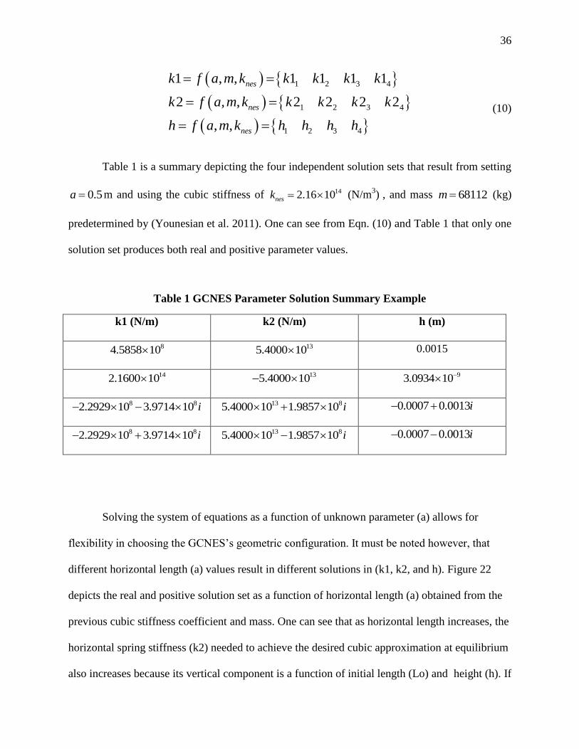
Table 1 is a summary depicting the four independent solution sets that result from setting
0.5a m and using the cubic stiffness of 142.16 10nesk (N/m3) , and mass 68112m (kg)
predetermined by (Younesian et al. 2011). One can see from Eqn. (10) and Table 1 that only one
solution set produces both real and positive parameter values.
Table 1 GCNES Parameter Solution Summary Example
k1 (N/m) k2 (N/m) h (m)
84.5858 10 135.4000 10 0.0015
142.1600 10 135.4000 10 93.0934 10
8 82.2929 10 3.9714 10 i 13 85.4000 10 1.9857 10 i 0.0007 0.0013i
8 82.2929 10 3.9714 10 i 13 85.4000 10 1.9857 10 i 0.0007 0.0013i
Solving the system of equations as a function of unknown parameter (a) allows for
flexibility in choosing the GCNES’s geometric configuration. It must be noted however, that
different horizontal length (a) values result in different solutions in (k1, k2, and h). Figure 22
depicts the real and positive solution set as a function of horizontal length (a) obtained from the
previous cubic stiffness coefficient and mass. One can see that as horizontal length increases, the
horizontal spring stiffness (k2) needed to achieve the desired cubic approximation at equilibrium
also increases because its vertical component is a function of initial length (Lo) and height (h). If

37
no variation in horizontal spring stiffness was apparent, the system’s total vertical force produced
about the equilibrium point would not equate to total gravitational force but would result in the
system’s dynamic motion along a linear tangent portion of the restoring force curve as described
in Figure 18.
Another interesting point is the plateau effect apparent in h and k1. As (a) increases,
vertical spring stiffness (k1) and initial height (h) tend to converge to a constant value due to
their lack of dependence on horizontal length in the vertical direction. Only relatively small
horizontal distances result in fluctuations of these two parameters that are most likely contributed
to a combination of the system’s geometric configuration and its cubic approximation
capabilities.
One can see from Figure 23 and Figure 24 that horizontal distance (a) is not only crucial
in choosing the device’s geometric configuration but its required dynamic performance in
application. Using the same mass and cubic stiffness coefficient, the maximum displacement that
can be obtained before a twenty percent deviation between the cubically approximated and the
complete GCNES restoring force is shown as a function of (a) in Figure 23. One can see that as
horizontal length increases, the maximum displacement obtained before said deviation tends to
be slightly more than half the initial horizontal length. Figure 24 shows the trend if a
displacement limitation, such as clearance height, was required. A value of 0.1 m was chosen to
represent such a limitation. One can see that below a minimum horizontal (a) range, the
difference between the two restoring forces diverge drastically with decreasing horizontal
lengths. Therefore, to achieve the desired dynamic effect and restoring force approximation,
some knowledge in the design stage regarding displacement ranges and geometric limitations is
crucial as the proposed device’s dynamic response can be greatly affected.

38
Figure 22 GCNES Parametric Solution Curves

39
Figure 23 Maximum Obtainable Displacement Before 20% Restoring Force Deviation
Example
Figure 24 Percent Difference Given Displacement Limitations Example

40
Figure 25 illustrates this concept even further by showing how the restoring force
deviates from the cubic approximation over a fixed displacement range using different horizontal
length (a) values and their associated solutions for (k1,k2, and h). One can see that, based on a
particular (a) value, the produced restoring force can be approximated cubically very precisely
but is limited by the displacement range over which this approximation holds true and tends to
deviate from the cubic approximation with larger displacements away from the static equilibrium
position. Therefore, it is necessary, in application and design, to be aware of both the geometric
and physical capabilities of the proposed GCNES device.
Figure 25 Restoring Forces with Multiple Horizontal Lengths Example

41
4. Two Degree of Freedom (2DOF) Oscillator Analysis
In this chapter, a simple two degree of freedom oscillator model is developed to analyze
and compare the gravitational force effects between a traditional linear and non-linear system’s
time history response. In addition, the capability of the GCNES system to compensate for gravity
is validated as well as its accuracy regarding a cubic restoring force approximation. For this
analysis, a linear TMD, an assumed cubic NES, and GCNES device are coupled to an undamped
linear oscillator.
Figure 26 shows the FBDs of each case respectively. Here, each system possesses a
primary mass (m1) of 1 kg with spring stiffness (k1) equal to 100 N/m, a device mass (mTMD,
mNES, or mGCNES) of 0.05 kg, and primary mass subjected to an impulsive load of 10 N for
approximately 0.005 s of the total simulation time. The TMD and NES cases are optimized for
primary mass displacement root mean squared (RMS) from 0 to 5 seconds, without applied
gravitational force, using the contour optimization process described in more detail in Chapter 6.
Optimization. Next, gravitational force is applied to both device and primary mass as a constant
load throughout the entirety of the simulation equivalent to the respective mass multiplied by g
(9.81 m/s2).
The GCNES case is then developed using the previously optimized cubic NES stiffness
coefficient (kNES) and its response under gravitational loading analyzed. One important note is
the implementation of initial conditions (u1(0) and u2(0)). In these simulations, the initial
displacement due to the addition of gravity on each DOF is implemented as an initial condition
in each system’s EOM. This allows for more accurate comparison between each cases dynamic
response and their resulting dynamic displacement RMS.

42
Figure 26 2DOF Schematic Diagrams: TMD (Left), Cubic NES (Center), and GCNES
(Right)
4.1 TMD 2DOF Analysis
The first scenario, described above, involves a traditional linear TMD. Eqn. (11) depicts
its EOM and the initial conditions solved for under gravitational loading. One can see by
comparing Figure 27 to Figure 28 that the addition of the gravitational force to both masses has
little to no effect in both the displacement and acceleration time history responses. This supports
the assumption that the change in static displacement due to gravity has little effect in a linear
restoring force relationship. In other words, regardless of the new static equilibrium point and
under constant gravitational loading, the device will still vibrate along a linearly proportional
force displacement relationship.

43
1 1 1 1 1 1
2 2 2
1
1
1
1
2
1
0 ( )
0
(0)
(0)
TMD TMD TMD TMD
TMD TMD TMD TMD TMD TMD
TMD
TMD TMD
TMD
m u c c u k k k u p t m g
m u c c u k k u m g
m g m gu
k
m g m g m gu
k k
(11)
Figure 27 TMD Impulse Time History Response without Gravity

44
Figure 28 TMD Impulse Time History Response with Gravity
4.2 NES 2DOF Analysis
The second 2DOF model described is an NES with an assumed cubic spring force
relationship shown in Eqn. (12). One unique feature in this EOM formulation is the addition of
the cubic spring force (FNES) to the force vector instead of the stiffness matrix. This is the
simplest method in accommodating non-linearity and allowed for direct implementation in the
Matlab ordinary differential equation (ODE) solver.
One can see by comparing Figure 29 to Figure 30 that the addition of gravitational force
has a significant effect on the NES’s performance in both the displacement and acceleration
responses. The NES response with gravity applied closely resembles the primary mass’s

45
response where little to no interaction with the NES is present. The NES rather, detunes and
responds similarly to a linear device with relatively high spring stiffness. This further supports
and validates the theory that gravity and the resulting change in static deflection cause the device
to vibrate about a position along the restoring force curve that resembles a linear-type
relationship. This results in the unintended high forces that are produced with larger
displacements from the new equilibrium point. Therefore, gravity and its effects are crucial in
design and application of vertical-type NES systems.
1 11 1 11
2 2 2
3
2 1
1
1
1
13
2
1
0 ( )0
0 0 0
(0)
(0)
NES NES NES
NES NES NES NES NES
NES NES
NES
NES NES
NES
m c c p t m g Fu u uk
m c c m g Fu u u
F k u u
m g m gu
k
m g m g m gu
k k
(12)

46
Figure 29 NES Impulse Time History Response without Gravity
Figure 30 NES Impulse Time History Response with Gravity

47
4.3 GCNES 2DOF Analysis
The third and final 2DOF model was formulated to validate the gravity compensating
capabilities of the proposed GCNES device. Its EOM, shown in Eqn. (13), was formulated using
the complete restoring force (FGCNES). The parameters (k1GCNES, k2GCNES, and h) were solved for
using the techniques described in Section 3.3 Device Realization and the NES model’s optimal
cubic stiffness coefficient value (kNES). Figure 31 and Figure 32 show that the addition of
gravitational force has little to no effect on the GCNES’s performance. The system’s
displacement and acceleration time history response accurately mimics the NES’s response
under no gravitational loading.
Figure 31 GCNES Impulse Solution Response as Function of Horizontal Length (a)

48
1 11 1 11
2 2 2
2 2 12 2 2
1 2 1 2 2 12
2
0 ( )0
0 0 0
2
GCNES GCNES GCNES
GCNES GCNES GCNES GCNES GCNES
GCNES GCNES GCNES
m c c p t m g Fu u uk
m c c m g Fu u u
h u uF k u u k a h a h u u
a h u u
2
1
1
1
1
2 1 2
(0)
(0) (0), (0) 0
GCNES
GCNES GCNES
m g m gu
k
u m g F u u
(13)
Additionally, it is apparent from Figure 31 that the response remains consistent and the
cubic approximation holds true for a wide range of solution sets. Horizontal length (a) values that
are relatively close to the device displacement ranges deviate slightly as solution sets closer to
those perform better and those that possess smaller (a) values perform slightly worse. This places
emphasis on the importance of parameter design and the displacement ranges discussed in
Section 3.3 Device Realization but also suggest a certain robustness for the GCNES device’s
parametric design.
Finally, Figure 33 shows the restoring force plotted as a function of relative
displacement. The simulation force curve was calculated using the simulation produced
acceleration values throughout the time history response. The actual force curve was calculated
using the parameters shown in the figure and the restoring force (FGCNES). One can see that the
two restoring force plots resemble each other closely and mimic a cubic curve providing both
validation in the implementation and simulation of the GCNES device’s cubic approximation.

49
Figure 32 GCNES Impulse Time History Response with Gravity
Figure 33 GCNES Impulse with Gravity Restoring Force Example
50
5. Floor Model
In this chapter, a relatively simple floor model is formulated using the assumed modes
method and the Lagrange equation. This floor model is used to compare the vertical vibration
mitigation capabilities of the proposed GCNES device. The device, coupled to the floor model, is
compared to both a control case, with no device, and with a traditional TMD attached. The
process used to derive the floor model as well as the assumptions made are described in the
following chapter.
5.1 Proposed Model
In order to preliminarily investigate the effectiveness of the GCNES at mitigating the
vertical vibration of a floor system, a simplified model of a flooring system was developed. This
model consists of a simply supported beam with an attached mass damper and subjected to a
vertical input force of a general form. Figure 34 depicts the floor model coupled with the
GCNES.

51
Figure 34 Floor beam model coupled to a GCNES device
Here, the resulting mass of the beam considered in the analysis is 1 kg/m. The modulus of
elasticity (E) and moment of inertia (I) of the beam are 1 Pa and 6.5 m4, respectively. In this
figure, xp is the loading position, p(t) is the load, xGCNES is the GCNES position, L is the span
length, mGCNES is the GCNES mass, ( , )u x t is the beam displacement, and x(t) is the GCNES
displacement. For the analysis, L = 1 m, xp = 0.3 m, and xGCNES = 0.65 m. The NES and GCNES
masses as well as the mass of a TMD located at the same point for comparison purposes is set to
5% of the mass of the flooring system.
These values were chosen not only for simplicity but to reflect the beneficial NES
attributes found throughout the literature review such as the positioning of the load (xp) and
placement of each device (xTMD, xNES, or xGCNES). While some of the model’s properties, such as
the mass and length, were set to unit values for simplicity, the model’s moment of inertia (I) was
scaled such that the beam possessed a fundamental frequency within the peak human perceptible

52
range (4-8Hz). All cases were subjected to an impulse loading (p(t)) of the form shown in Eqn.
(14).
210sin , 0
2( )
0,2
p
p
p
Ttt
Tp t
Tt
(14)
This half sine pulse is similar to the loading used in the study conducted by (Georgiades and
Vakakis 2007). This study, however, used the new fundamental period Tp = 0.2497 s found from
the control cases’s eigenvalue analysis that is described in section (5.4 Modal Analysis &
Damping Matrix). Each case’s respective equation of motion (EOM) formulation is described in
greater detail in the Lagrange Formulation section (5.3 Lagrange Formulation) of this document.
5.2 Assumed Modes Method
As previously mentioned, the assumed modes method was used to estimate and derive
each case’s respective EOM. This method is commonly used to model the dynamics of
continuous systems. In order to model these dynamics, the five shape functions shown in
functional form in Table 2 are used. It is known that the closer these shape functions are to the
actual vibration mode, the more accurate the results are from this analysis will be. With this in
mind, the five assumed shape functions for this floor model were chosen based on a sine wave
function, which has been previously shown to be able to model a homogenous simply supported
beam effectively (Georgiades and Vakakis 2007; Younesian et al. 2011). While the presence of
the mass dampers considered will cause the considered system to deviate, this set of shape
functions is still expected to perform well.

53
Table 2 Assumed Shape Functions
Assumed Shape Function Variables Functional Form
Ψ1 sinx
L
Ψ2
2sin
x
L
Ψ3 3
sinx
L
Ψ4 4
sinx
L
Ψ5 5
sinx
L
The shape functions considered are mathematically valid given that they satisfy the basic
criteria required for their use in the assumed modes method. The first criteria that must be
satisfied are the general boundary conditions. Given that the floor model is a simply supported
beam, the assumed shape functions must result in zero displacement about the points where L =
0 and L = L. One can see from Table 2 that inserting either x = 0 or x = L into any of the shape
functions satisfies these criteria. Eqn. (15) shows an example for the first shape function (Ψ1).
(0)sin sin 0 0
( )sin sin 0
L
or
L
L
(15)
The second criteria is that the assumed shape functions must possess a number of
derivatives that are greater than or equal to the number of derivatives found in the system’s strain
energy function. The model of the beam’s strain energy expression used herein contains two

54
derivatives. One can see from Eqn. (16) that taking the first and second derivatives of the first
shape function (Ψ1) results in two valid expressions that satisfy the required amount of
derivatives needed to use this method. Furthermore, it should be noted that the sinusoid shape
functions utilized have an unlimited number of non-zero derivatives.
1
22
1
cos
sin
d x
dx L L
and
d x
dx L L
(16)
The third criteria the assumed shape functions must possess is that they must be linearly
independent. This requirement is automatically satisfied for functions with the form sinn x
L
.
Figure 35 shows each assumed shape function plotted along the floor beam’s length. As
one can see from the figure, each function takes significantly different forms. This is a desired
characteristic when using the assumed modes method as it allows for more accurate
representation of the system’s dynamic response.
With the assumed modes method, the degrees of freedom computed as the computational
response are the scaling values applied to each shape function. To represent the physical
response, the desired output is a combination of all the shape functions and their corresponding
scaling factors at specific points in the system. In this model, for example, the computational
model’s dynamic response at the beam’s midspan (L = L/2) would be equal to the summation of
each degree of freedom’s (DOF) output scaled by the corresponding shape function’s resulting
value at a specific point along the beam. Eqn. (17) depicts this relationship.

55
1
,2 2
n
i i
i
L Lu t q t
(17)
In this equation, the desired time history displacement response at the beam’s midspan
( / 2)L L is represented by / 2,u L t where i is the related shape function and iq is its
corresponding DOF.

56
Figure 35 Assumed shape functions plotted along beam length

57
5.3 Lagrange Formulation
In this chapter, the Lagrange Equation was used to derive each respective case’s EOM.
As previously mentioned, the assumed modes method was used to estimate the first five modes
for the beam without a mass damper, which results in the beam having five degrees of freedom.
The sixth DOF results from the attached device for both the TMD, NES, and GCNES cases. The
Lagrange Equation is depicted in Eqn. (18) where T represents the system’s total kinetic energy
expression, V represents the system’s total potential energy expression, qi represents the
corresponding DOF, and pi represents the non-conservative virtual work term associated with the
corresponding DOF’s virtual displacement δqi.
( )i i
i i i
d T T Vp t q
dt q q q
(18)
Using this formula, the EOM for each DOF can be derived and compiled into matrix
form. First, however, expressions for the floor model’s three respective cases need to be
developed. The detailed formulation of each case’s potential energy, kinetic energy, and non-
conservative virtual work expressions are described in the following subsections.

58
Control Case Formulation
Figure 36 Floor beam model control case diagram
Figure 36 depicts the floor model without any device attached. The model in this
configuration is considered as the control case throughout the remainder of this document. In
addition, this case’s resulting EOM is used to perform the modal analysis and derive the modal
damping matrix described in section (5.4 Modal Analysis & Damping Matrix).
In order to use the Lagrange Equation, shown in Eqn. (18), an expression for the floor
model’s total kinetic energy needs to be developed. Eqn. (19) is essentially the total kinetic
energy produced by the floor beam’s mass at a point (x) along the beam’s length and integrated
throughout the entire beam length to produce an effective beam mass. In this expression, ,u x t
represents the system’s velocity as a function of space and time and iq t represents the ith
DOF
velocity as a function of time resulting from the assumed modes method formulation.

59
2
0
2
10
1,
2
1( ) ( )
2
L
L n
i i
i
T A u x t dx
T A x q t dx
(19)
Similarly, the floor beam’s total potential energy expression is depicted in Eqn. (20).
Here, the floor beam’s total potential energy is expressed as a function of the total system
displacement’s second spatial derivative , ''u x t (note that the displacement is a function
with respect to both space and time), which is a direct mathematical expression for the equivalent
stiffness of a beam at a specific point along its length. The need for the second spatial derivative
is a result of calculating the slope of the beam’s stiffness relationship, which is then integrated
along the entire beam length to produce effective beam stiffness. This equation is further
represented as a function of the ith
DOF displacement iq t with respect to time resulting from
the assumed modes method formulation.
2
''
0
2
''
10
1,
2
1( ) ( )
2
L
L n
i i
i
V EI u x t dx
V EI x q t dx
(20)
The floor model’s non-conservative virtual work expression (δWNC) is shown in Eqn.
(21). This expression is related to the components of a dynamic system that either add or subtract
energy from the system. Components such as dampers, applied forces, and sometimes spring

60
forces are expressed in terms of their virtual displacements and the virtual work they perform on
the system. The overall damping of the beam will be considered separately; thus, for the control
case, the only contributor to this expression is the external load applied to the floor beam (p(t)).
In Eqn. (21), this force is represented in terms of beam virtual displacement ,pu x t with
respect to time and at the location of the load. Using the assumed methods formulation, this
expression is further represented in terms of the ith
DOF virtual displacement (δqi(t)) with respect
to time. Here, the virtual displacement term is also evaluated spatially at the positioning of the
loading (xp).
1
( ) ,
( )
NC p
n
NC i p i
i
W p t u x t
W p t x q t
(21)
Inputting these three expressions into Eqn. (18), performing the necessary mathematical
operations, and rearranging into matrix format yields the floor beam model’s EOM without any
device attached (control case). One can see that the system’s global mass matrix [M] (Eqn. (22))
results from the kinetic energy expression (T).
2
1 1
0 0
1
0 0
L L
m
L L
n n m
A x dx A x x dx
M
A x x dx A x x dx
(22)

61
The global stiffness matrix [K] (Eqn. (23)) is a result of the potential energy expression (V).
2'' '' ''
1 1
0 0
'' '' '' ''
1
0 0
L L
m
L L
n n m
EI x dx EI x x dx
K
EI x x dx EI x x dx
(23)
The force vector [P] (Eqn. (24)) is derived from the non-conservative virtual work expression
(δWNC).
1
( )
p
n p
x
P p t
x
(24)
Finally, these expressions, once compiled into matrix format, are represented by Eqn. (25).
1 1 1
n n n
q q q
M C K P
q q q
(25)
It should be noted that this equation contains a damping matrix [C]. The derivation of this
matrix, for the control case, is described in section (5.4 Modal Analysis & Damping Matrix).
This matrix is a direct result of performing a modal analysis on the floor model and assuming 1%
damping in each beam mode. For simplicity, it is represented as a variable here but will be used

62
in latter portions of this work to represent the realistic behavior of a beam containing some form
of natural damping.
It should also be noted that the EOM depicted in Eqn. (25) is of the form represented by
the assumed modes method DOF acceleration, velocity, and displacement variables
, ,and i i iq t q t q t . In order to convert these DOF values back into the system’s physical
coordinates , , , , ,u x t u x t and u x t , the assumed modes vectors are multiplied by vectors
containing the assumed shape functions. Essentially, the resulting physical coordinate value at
the spatial position (x) is calculated by multiplying the assumed modes vector with the shape
function vector evaluated at the same position. Eqn. (26) represents the process of converting the
assumed modes DOF displacement into physical displacement at the beam’s midspan (L/2).
1
1,2 2 2
n
n
qL L L
u t
q
(26)

63
TMD Case Formulation
Figure 37 Floor beam model coupled with TMD diagram
For the case where the floor model is coupled to a TMD device (Figure 37), the kinetic
energy expression (T) possesses an additional term, shown in Eqn. (27), that represents the
kinetic energy of the attached TMD mass. In this expression, TMDm represents the mass of the
TMD device and x t represents the coupled device’s velocity with respect to time. The
resulting mass matrix is depicted in Eqn. (28).
2 2
0
2
2
10
1 1,
2 2
1 1( ) ( )
2 2
L
TMD
L n
i i TMD
i
T A u x t dx m x t
T A x q t dx m x t
(27)

64
2
1 1
0 0
1
0 0
0
0
0 0
L L
m
TMD L L
n n m
TMD
A x dx A x x dx
M
A x x dx A x x dx
m
(28)
Furthermore, this model includes an additional term in the potential energy expression
(Eqn. (29)). This term is a direct result of the TMD’s linear spring restoring force and is a
function of the TMD’s spring constant TMDk and the relative value between the beam’s
displacement ,TMDu x t , evaluated at the position of the TMD device spatially, and the
device’s displacement x t with respect to time. The resulting stiffness matrix is depicted in
Eqn. (30).
2 2''
0
2 2
''
1 10
1 1, ( ) ,
2 2
1 1( ) ( ) ( )
2 2
L
TMD TMD
L n n
i i TMD i TMD i
i i
V EI u x t dx k x t u x t
V EI x q t dx k x t x q t
(29)
2
1 1 111 1
11
1
TMD TMD TMD TMD m TMD TMD TMDm
TMD
TMD n TMD TMD TMD n TMD m TMD TMD m TMDn nm
TMD TMD TMD m TMD TMD
K k x K k x x k x
KK k x x K k x x k x
k x k x k
(30)
The non-conservative virtual work expression also contains an addition in the form of the
TMD’s linear viscous damper force dF . This force, depicted in Eqn. (32), is a function of the

65
TMD’s damping coefficient TMDc and the relative velocity between the beam and device. In
Eqn. (31), the additional term is a product of the device’s damper force and the relative virtual
displacement of the beam, evaluated at the position of the device along the beam, and the
device’s virtual displacement x t with respect to time.
1 1
( ) , ,
( )
NC p d TMD
n n
NC i p i d i TMD i
i i
W p t u x t F x t u x t
W p t x q t F x t x q t
(31)
1
,d TMD TMD
n
d TMD i TMD i
i
F c x t u x t
F c x t x q t
(32)
Finally, the necessary mathematical operations, depicted in Eqn. (18) along with the
matrix compilation process, are performed to obtain the TMD case’s EOM. It should be noted
that this process, unlike the control case, results in the addition to the damping matrix [C]. This
matrix is a direct result of the device’s linear damping force dF and takes the form shown in
Eqn. (33). One can see that the final resulting EOM shown in Eqn. (34) results in a DOF addition
to account for the inclusion of the device.
2
1 1 1
1
1 1
TMD TMD m TMD TMD
TMD TMD
n TMD TMD n TMD m TMD n TMD
TMD m TMD
x x x x
C c Cx x x x x
x x
(33)

66
11 1 1
( )
0
p
TMD TMD TMD
n n n n p
xq q q
M C K p tq q q x
x x x
(34)
NES Case Formulation
Figure 38 Floor beam model coupled with NES diagram
The formulation of the floor model, coupled with the NES device, follows the same
process as both the control and TMD cases. This case’s total kinetic energy expression (T) is
identical to the TMD case with the renaming of the TMD mass as the NES mass NESm , for
clarity. Also, this case’s potential energy expression (V) is identical to the control case’s
67
expression with the inclusion of the additional DOF. The TMD damping coefficient is also
renamed to represent the NES damping coefficient NESc .
The only change is apparent in the non-conservative virtual work expression. In this
expression, the non-linear stiffness force produced by the NES device takes the form depicted in
Eqn. (36). While the cubic force from the NES stiffness element is conservative, it is considered
in this stage because it is being evaluated as an external force from the NES to the beam. Here,
the force NESF is represented as the product of the NES device’s spring coefficient NESk ,
shown in Eqn. (9), and the relative displacement between the beam, evaluated at the spatial
position of the device NESx , and the device’s displacement with respect to time cubed. Eqn.
(35) represents this force’s inclusion into the non-conservative virtual work expression as the
product between itself and the relative virtual displacement between the beam and coupled
device. The final resulting EOM can be seen in Eqn. (37).
1
,NES NES
n
NES i NES i
i
F x t u x t
F x t x q t
(35)
3
3
1
,NES NES NES
n
NES NES i NES i
i
F k x t u x t
F k x t x q t
(36)

68
11 1 1 1
( )
10
pNES
NES NES NES NES
n n n n NESn p
xq q q x
M C K p t Fq q q xx
x x x
(37)
GCNES Case Formulation
Using Figure 34, the EOM can be derived for the GCNES case. For this case, the
potential and kinetic energy expressions are identical to that of the NES case. The only exception
is found in its non-conservative virtual work expression (δWNC). Eqn. (38) depicts the full
expression for the GCNES force (FGCNES) that is included. Also, each global matrix and
appropriate device variable has been renamed for clarity between all four cases. The resulting
EOM is depicted in Eqn. (39).
1
22 2 2
22
2
1
1
2
12 2 2
2
1
,
,2 ,
,
2
GCNES GCNES
GCNES
GCNES
GCNES
n
GCNES i GCNES i
i
n
i GCNES ini
i GCNES i
i
F k x t u x t
h x t u x tk a h a h x t u x t
a h x t u x t
F k x t x q t
h x t x q t
k a h a h x t x q t
2
2
1
n
i GCNES i
i
a h x t x q t
(38)
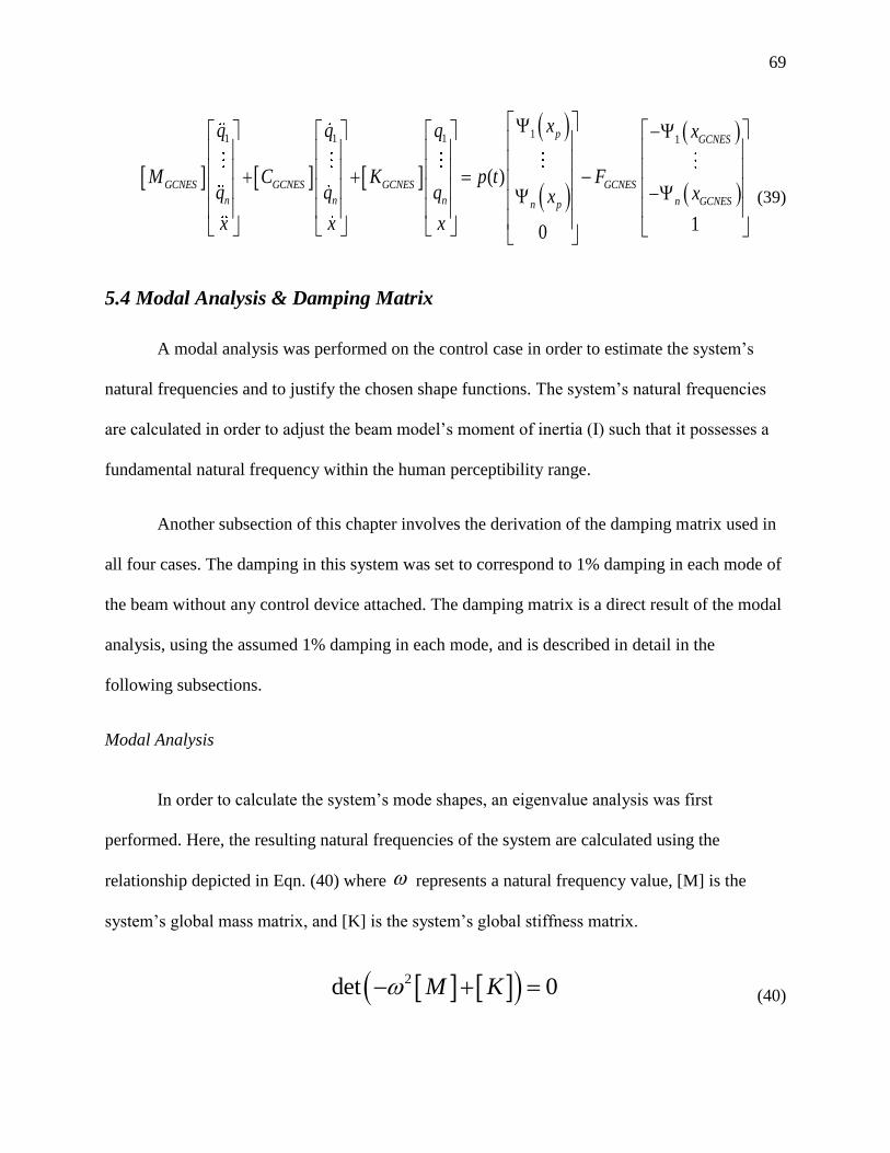
69
11 1 1 1
( )
10
pGCNES
GCNES GCNES GCNES GCNES
n n n n GCNESn p
xq q q x
M C K p t Fq q q xx
x x x
(39)
5.4 Modal Analysis & Damping Matrix
A modal analysis was performed on the control case in order to estimate the system’s
natural frequencies and to justify the chosen shape functions. The system’s natural frequencies
are calculated in order to adjust the beam model’s moment of inertia (I) such that it possesses a
fundamental natural frequency within the human perceptibility range.
Another subsection of this chapter involves the derivation of the damping matrix used in
all four cases. The damping in this system was set to correspond to 1% damping in each mode of
the beam without any control device attached. The damping matrix is a direct result of the modal
analysis, using the assumed 1% damping in each mode, and is described in detail in the
following subsections.
Modal Analysis
In order to calculate the system’s mode shapes, an eigenvalue analysis was first
performed. Here, the resulting natural frequencies of the system are calculated using the
relationship depicted in Eqn. (40) where represents a natural frequency value, [M] is the
system’s global mass matrix, and [K] is the system’s global stiffness matrix.
2det 0M K (40)

70
The resulting eigenvalues i that satisfy the relationship above are the resulting
system’s natural frequencies. Table 3 outlines all calculated natural frequencies for the control
case only. It should be noted that the eigenvalue analysis was performed on this case in order to
accurately estimate the floor model’s natural frequencies without any device attached.
Table 3 Fundamental natural frequencies
Natural Frequency of ith
Mode (ωi) (rad/s) (Hz)
ω1 25.13 4.00
ω2 100.66 16.02
ω3 226.45 36.04
ω4 402.63 64.08
ω5 629.07 100.12
Mode Shapes
Using the previously calculated natural frequencies, the system’s resulting mode shapes
can be plotted by substituting in each natural frequency i into Eqn. (41).
2 0i M K (41)
In this equation, [ϕ] represents the mode shape vector where each element corresponds to the
system’s respective DOF. This system of equations is then solved for by assuming a convenient
value for one element in the mode shape vector and solving the remaining equations
simultaneously. Once plotted, the result is a scaled version of the shape the system takes while
vibrating at the corresponding mode.

71
For this system, the assumed element value in the mode shape vector [ϕ] was taken as
one for the corresponding mode in question. In other words, solving for the 3rd
mode required the
third element to equal one as shown in Eqn. (42). This value was chosen for its simplicity in
solving the system of simultaneous equations, described previously, as it eliminates the need to
solve for one of the unknown mode shape vector elements and scales the remaining elements
around the assumed value. For example, Eqn. (42) depicts the relationship used in solving for the
elements in the third mode shape vector 3 where 31 denotes the first element in the third
mode shape vector.
31
32
2
3
3
1 0
n
M K
(42)
Once each mode shape vector is solved for, the corresponding physical mode shape is the
result of multiplying the mode shape vector with a vector of the assumed shape functions as
depicted in Eqn. (43). Here, MS1(x) represents the first physical mode shape as a function of the
floor model’s beam length, Ψi(x) is the assumed shape function for the ith
mode, and ϕ11
represents the first element in the first mode shape vector [ϕ].
11
1 1
1
S n
n
M x x x
(43)

72
The mode shapes are then plotted as a function of the floor model’s beam length. The
resulting mode shapes for the floor model are depicted in Figure 39. As one can see by
comparing Figure 35 and Figure 39, the first assumed mode shape is practically identical to the
system’s actual mode shape. In addition, the remaining assumed mode shapes are fairly accurate
representations of the system’s actual vibration modes, with only minor discrepancies. This
supports the use of the previously described assumed shape function forms and validates an
accurate representation of the floor model’s natural forms of vibration without any device
attached.

73
Figure 39 Modal analysis mode shapes plotted along beam length

74
Damping Matrix
The floor model’s damping matrix was derived using the concept of modal superposition.
Modal superposition is a method used to define a system’s physical coordinates as a function of
its mode shapes and a set of modal coordinates. This method produces a decoupled system of
single degree of freedom (SDOF) EOMs that result from an original multi degree of freedom
(MDOF) system. In general, a damping matrix can be derived using this technique, as
represented by Eqn. (44), where C is referred to as the modal damping matrix and is a
matrix containing all mode shape vectors .
TC C
(44)
The modal damping matrix is assumed to be diagonal in nature as all matrices, in modal form,
must be diagonal in order to represent the decoupled SDOF EOMs. Therefore, the modal
damping matrix’s elements, shown by Eqn. (45), correspond to each of the system’s DOFs.
1 0 0
0 0
0 0 n
C
C
C
(45)
Using this relationship, one can see, from Eqn. (46), that each modal damping element
iC is a function of its corresponding DOF’s viscous damping coefficient i , natural
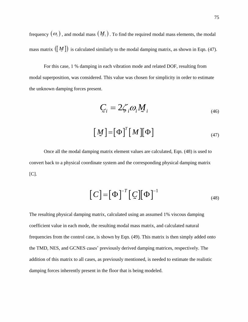
75
frequency i , and modal mass iM . To find the required modal mass elements, the modal
mass matrix M is calculated similarly to the modal damping matrix, as shown in Eqn. (47).
For this case, 1 % damping in each vibration mode and related DOF, resulting from
modal superposition, was considered. This value was chosen for simplicity in order to estimate
the unknown damping forces present.
2i i i iC M
(46)
T
M M (47)
Once all the modal damping matrix element values are calculated, Eqn. (48) is used to
convert back to a physical coordinate system and the corresponding physical damping matrix
[C].
1T
C C
(48)
The resulting physical damping matrix, calculated using an assumed 1% viscous damping
coefficient value in each mode, the resulting modal mass matrix, and calculated natural
frequencies from the control case, is shown by Eqn. (49). This matrix is then simply added onto
the TMD, NES, and GCNES cases’ previously derived damping matrices, respectively. The
addition of this matrix to all cases, as previously mentioned, is needed to estimate the realistic
damping forces inherently present in the floor that is being modeled.

76
0.2516 0 0 0 0
0 1.0065 0 0 0
0 0 2.2646 0 0
0 0 0 4.0260 0
0 0 0 0 6.2907
C
(49)

77
6. Optimization
In order to obtain the optimal parameters for both the 2DOF and Floor Model analysis,
Matlab Software, using a strong ODE solver, and a simple contour optimization method were
introduced. This process involved looping each simulation over a wide range of damping and
stiffness coefficients as simulation inputs. The minimum constraint or minimum response could
then be visually identified on a graph.
Here Figure 40 and Figure 41 represent TMD and NES optimal stiffness and damping
parameters used in the 2DOF analysis. The minimum displacement RMS response throughout
the entire twenty second simulation time was acquired. It should be noted that the TMD
optimization produces relatively uniform contours while the NES can be unpredictable and
require much larger stiffness values for effectiveness. This represents one of the many challenges
in optimizing a non-linear system justifying the need for even a simplistic cubic approximation
as described in this document. This lends credit to the ability of the complex GCNES restoring
force to be approximated with the cubic restoring force.
Figure 42 and Figure 43 show the contour plots for the TMD and NES produced using
the same process. The minimum displacement RMS from zero to two seconds was acquired for
these simulations. The same aforementioned phenomena regarding non-uniform variation with
the NES case can be seen as well.

78
Figure 40 TMD 2DOF Contour Optimization

79
Figure 41 NES 2DOF Contour Optimization
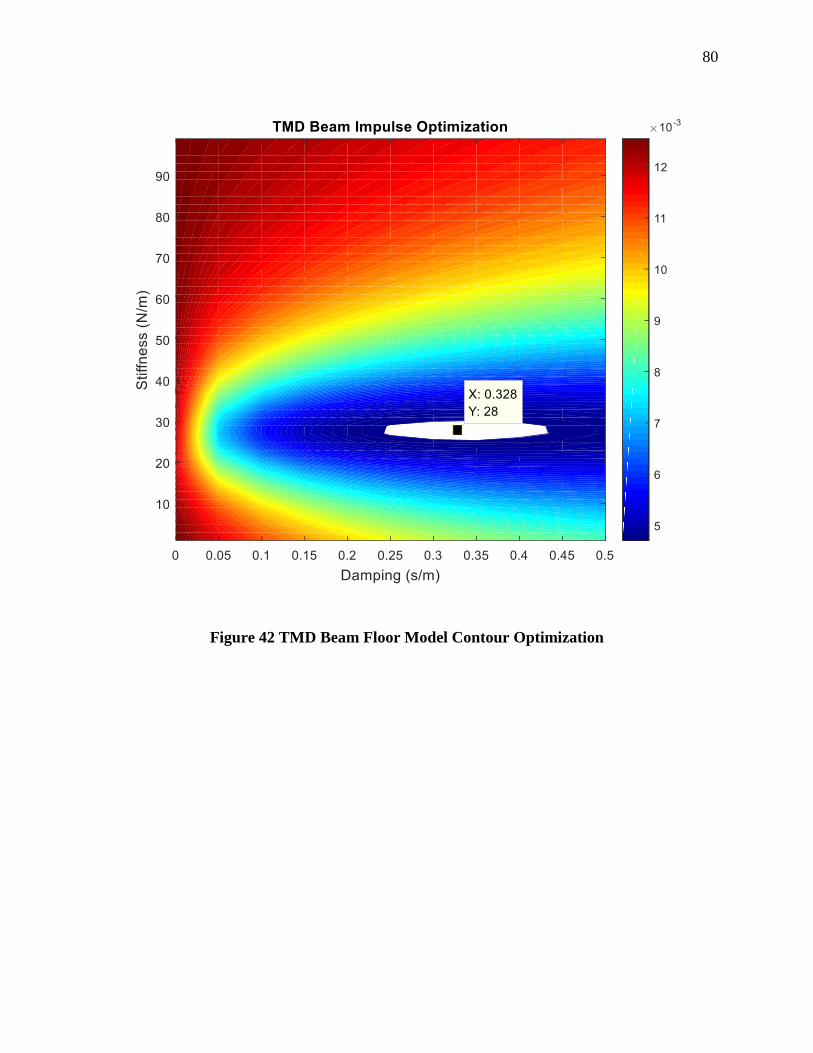
80
Figure 42 TMD Beam Floor Model Contour Optimization

81
Figure 43 NES Beam Floor Model Contour Optimization

82
7. Beam Model Vibration Mitigation
In this chapter, the findings from all four cases simulated using the beam floor model are
presented. These cases include the control, with no device attached, the TMD, NES, and
GCNES. The effectiveness of the TMD and the non-linear attachments is examined in a variety
of scenarios that deviate from the optimized conditions. Each of these scenarios mimics the
conditions that could occur in a flooring system. Perhaps more importantly, the GCNES’s ability
to compensate for the effect of gravity is also presented under the same scenarios with the
inclusion of gravitational force.
7.1 Control Impulse Excitation Response
This section describes in detail both the floor model’s response with no device and the
justification behind the optimized parameters discussed in Chapter 6. Optimization. Each
analysis was simulated for a total duration of twenty seconds and subjected to the impulse
loading shown in Eqn. (14) and described in detail by section 5.1 Proposed Model. This duration
was chosen as it is apparent from Figure 44 that the beam’s response is nearly completely
damped at a time t = 20 s. Consideration of the beam’s response at its midspan in this analysis
was chosen based on its tendency to become a maximum in the systems fundamental mode of
vibration, which is apparent from Figure 35 and Figure 39.
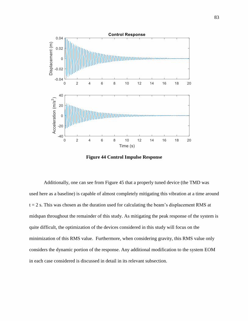
83
Figure 44 Control Impulse Response
Additionally, one can see from Figure 45 that a properly tuned device (the TMD was
used here as a baseline) is capable of almost completely mitigating this vibration at a time around
t = 2 s. This was chosen as the duration used for calculating the beam’s displacement RMS at
midspan throughout the remainder of this study. As mitigating the peak response of the system is
quite difficult, the optimization of the devices considered in this study will focus on the
minimization of this RMS value. Furthermore, when considering gravity, this RMS value only
considers the dynamic portion of the response. Any additional modification to the system EOM
in each case considered is discussed in detail in its relevant subsection.

84
Figure 45 Optimal Response Justification Example
7.2 Control, TMD, and NES Case Comparisons
Once the aforementioned minimum response criteria was established using the optimal
TMD mitigation effectiveness as the standard, the NES and GCNES cases could be examined. In
this section, gravity is not considered explicitly; therefore, the results for the NES shown can be
considered as the results expected with a GCNES if gravity was present.
TMD Optimal Response
From Figure 46, one can see that the optimal TMD time history response shows excellent
performance within the initial two second duration. The device limits the initial displacement
RMS to 0.0103 m. One can also see from the figure that the TMD experiences a peak in device
response followed by a progressive, damped motion for the remainder of the simulation.

85
Figure 46 TMD Optimal Response
NES Optimal Response
One can see from Figure 47 that the properly tuned NES also completely damps the
beam’s response at a time duration of approximately two seconds. Although the TMD performs
slightly better, the NES still performs adequately by limiting the beam’s displacement RMS
response to 0.0113 m. One interesting characteristic noticeable in the NES response is an
equivalent peak in the device’s motion not seen in the TMD analysis. This suggests that at
different time values, the NES is still experiencing equivalent amounts of motion and producing
equivalent amounts of force as previous time values. This is characteristic to a non-linear
response performance. In addition, having both devices perform within the same time duration
lends support to this work’s optimal parameter obtainment methods.

86
Figure 47 NES Optimal Response
Parameter Response Analysis
Furthermore, each case was simulated using a variety of scenarios that might occur in a
typical flooring system. For these investigations, each system’s device parameters discussed
previously were not adjusted in order to reoptimize and account for these changes. Rather, the
parameters are left constant in order to test the robustness needed from a solely, passive system
in a real world environment. Figure 48 shows the response variation between the control, TMD,
and NES cases with changing load amplitude. One can see from the figure that the control and
TMD possess typical linear responses that are scaled with amplitude, while the NES has a
nonlinear response about the optimized 10 N amplitude. This behavior is expected as the NES
being a nonlinear device is known to have amplitude dependent behavior. Although the NES

87
does not outperform the TMD at any amplitude, the NES and the TMD have similar responses
over a wide range of load amplitude considered. This shows that, despite being nonlinear, the
NES performance can show some robustness under changing load environments.
Figure 49 shows the response variation when the respective devices are moved to
different locations along the beam. This plot suggests, under constant load conditions, each
device is inherently more effective at mitigation of the beam’s midspan when placed near to that
point. Figure 50 compares the response when the loading location is changed. One interesting
aspect regarding this figure is the NES’s tendency to be more effective when the loading is near
the beam’s third points which supports the findings of (Georgiades and Vakakis 2007).
Figure 48 Amplitude Response Comparison

88
Figure 49 Device Position Response Comparison
Figure 50 Load Position Response Comparison

89
Lumped Mass Analysis
Finally, several scenarios in particular were developed to mimic variation in the floor
beam’s mass. This scenario is very prevalent in flooring systems, especially in structures that are
intended for multifunctional use or retrofitted for reuse. In order to subject the beam model to
these conditions, the addition of a lumped mass on the beam was derived. Given that this lumped
mass was not considered as an additional DOF but an increase in the beam’s mass at a certain
location, the only difference in each cases’s EOM can be found in the kinetic energy expression
(T). This expression is shown by Eqn. (50) where mDevice represents each respective device mass,
madd represents the additional mass value (kg), and xm represents the lumped mass’s location
along the beam. The resulting addition to each system’s global mass matrix [M] is illustrated by
Eqn. (51).
2 22
0
2 2
2
1 10
1 1 1, ,
2 2 2
1 1 1( ) ( ) ( ) ( )
2 2 2
L
Device add m
L n n
i i Device add i m i
i i
T A u x t dx m x t m u x t
T A x q t dx m x t m x q t
(50)
2
1 1
1
0
0 0
add m add m m m
add n m m add n m m m
m x m x x
m x x m x x
(51)
One of the more interesting relationships is illustrated in Figure 51. One can see that a
lumped mass equivalent to approximately 15 % of the beam’s mass and higher, located at
midspan, causes the TMD to detune and converge towards the control response. The NES, on the
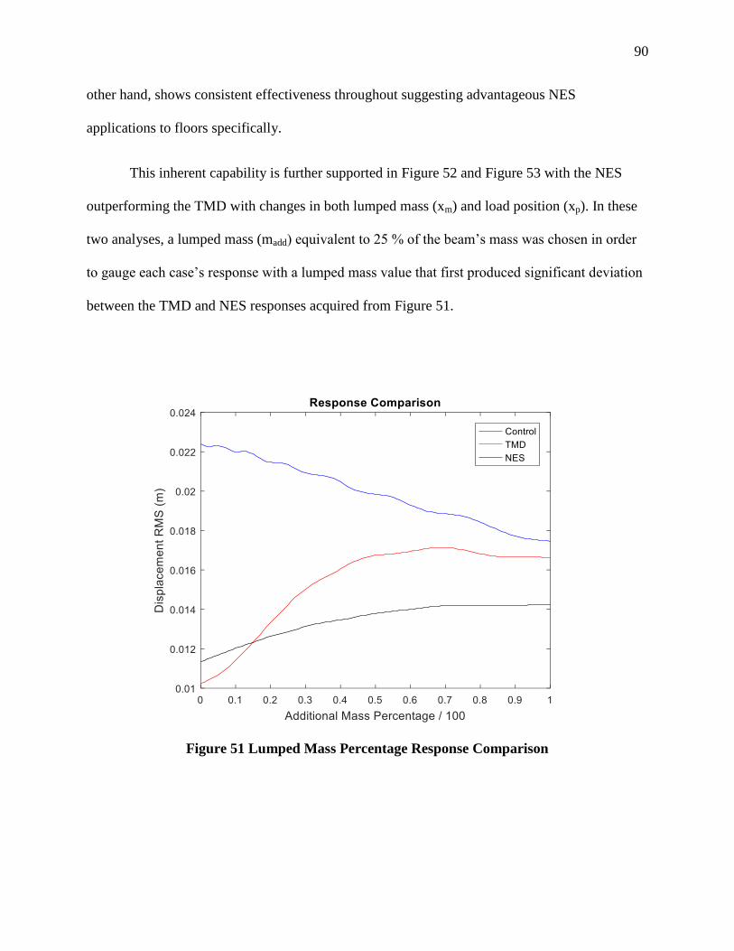
90
other hand, shows consistent effectiveness throughout suggesting advantageous NES
applications to floors specifically.
This inherent capability is further supported in Figure 52 and Figure 53 with the NES
outperforming the TMD with changes in both lumped mass (xm) and load position (xp). In these
two analyses, a lumped mass (madd) equivalent to 25 % of the beam’s mass was chosen in order
to gauge each case’s response with a lumped mass value that first produced significant deviation
between the TMD and NES responses acquired from Figure 51.
Figure 51 Lumped Mass Percentage Response Comparison

91
Figure 52 25% Lumped Mass Position Response Comparison
Figure 53 Load Position with 25% Lumped Mass Response Comparison

92
To better understand what is happening under these conditions, the time history responses
for the lumped mass (madd) equivalent to 25 % of the beam’s located at midspan are given in
Figure 54, Figure 55, and Figure 56. By comparing these figures, one can see that the TMD
device’s response is converging toward the control cases’s response. The TMD is therefore,
beginning to detune, and ultimately, as additional mass increases, become less and less effective
at mitigation.
Figure 54 Control 25% Lumped Mass Response

93
Figure 55 TMD 25% Lumped Mass Response
This convergence, however, is not apparent in the NES response which suggests energy
is still able to be absorbed. A close inspection of the device’s motion yields larger variation in
device displacement compared to its optimal response but contained within the same time
duration. This supports the assumption that energy is being irreversibly transferred between the
device and beam. Finally, Figure 57 provides a clear comparison in the beam’s response under
each case showing optimal effectiveness provided by the NES.
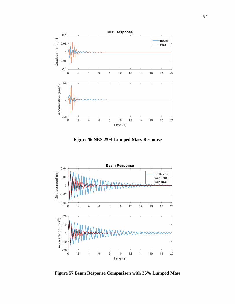
94
Figure 56 NES 25% Lumped Mass Response
Figure 57 Beam Response Comparison with 25% Lumped Mass

95
7.3 GCNES Gravity Compensation
In this section, the findings reported in section 7.2 Control, TMD, and NES Case
Comparisons are analyzed with the inclusion of gravitational force. In addition, the GCNES case
is analyzed with the goal of mimicking the advantageous, NES response characteristics. In order
to gauge the GCNES’s effectiveness, the optimal solutions were obtained and used for the
remainder of the simulations. Figure 58 shows the variation in beam response as a function of the
device’s horizontal length (a), which is one of the choices when designing the parameters of this
device. One can see that roughly beyond a = 0.1 m the response converges and is relatively
unaffected by the solution set used. Certain lengths below this threshold perform significantly
worse due to their displacement limitation and resulting inability to approximate the cubic
relationship needed.
Figure 58 GCNES Parameter Response as Function of Horizontal Length

96
Gravitational force was applied to each case’s device mass, respectively, via a constant
point load equivalent to the device mass (mDevice) multiplied by 9.81 m/s2. Additionally,
appropriate initial conditions were applied and solved for using the methods introduced in
Chapter 4. Two Degree of Freedom (2DOF) Oscillator Analysis such that each analysis begins
with the device and beam in their at rest positions. Figure 59 shows the GCNES’s time history
response under optimal conditions using the solutions obtained from the NES’s optimized cubic
stiffness coefficient. One can see that the response precisely resembles the NES response not
considering gravity, which is shown in Figure 47. This supports the GCNES’s gravity
compensation capabilities and validates its application to these types of scenarios.
Figure 59 GCNES Optimal Response

97
For better comparison and justification, all four cases were subjected to the applied
gravitational force and their responses investigated. Figure 60 illustrates both the GCNES’s
effectiveness and the importance of considering the effects due to gravity in vertical, non-linear
applications. It is clear that in the linear control and TMD responses are unaffected by gravity.
The NES, however, becomes progressively worse and deviates significantly from its beneficial
performance as the amount of added mass is increased. This is also reflected in the scenarios
depicted in Figure 61 and Figure 62. The GCNES shows an overall better performance than all
of the other systems considered. Critically, this GCNES performance precisely approximates the
NES’s response under no gravitational force (see Figure 51). This result further validates the
GCNES’s cubic approximation capability, solution obtainment methods, and overall
effectiveness in vertical vibration mitigation applications.
Figure 60 Lumped Mass Percentage Response Comparison (Gravity Considered)
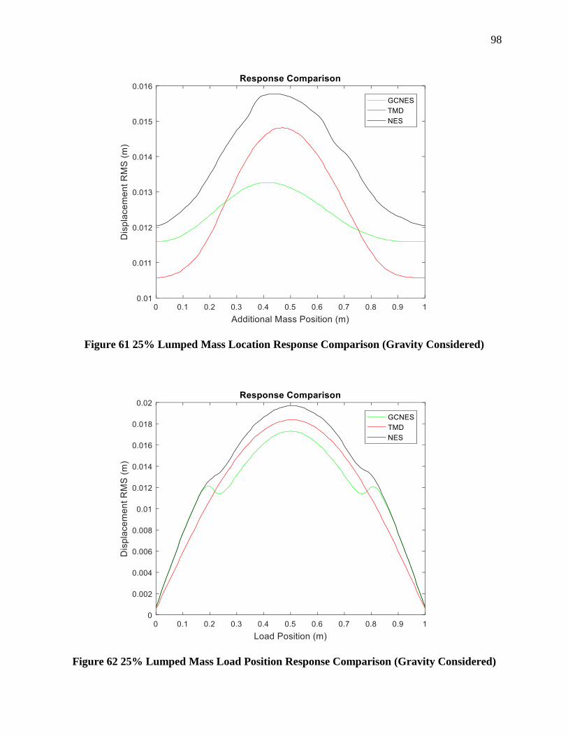
98
Figure 61 25% Lumped Mass Location Response Comparison (Gravity Considered)
Figure 62 25% Lumped Mass Load Position Response Comparison (Gravity Considered)

99
8. Realistic GCNES Design
In this chapter, practical implementation of the GCNES device is investigated. Primarily,
the feasibility to physically construct the required stiffness parameters using structural steel is
presented. An interior floor girder with section properties commonly used in thin composite
steel-concrete structures is analyzed herein under an impulsive load with the aforementioned
beam model, optimization technique, and GCNES design method. A complete design example
for this flooring system (without a vertical vibration suppression device) is illustrated and
described in the references (Wanant 2014).
Figure 63 Steel-Concrete Composite Deck Girder (Wanant 2014)
For this analysis, the floor system possessed a dead load equal to 60 psf and a reduced
live load equal to 45.3 psf in an office building with 28 x 28 ft column line dimensions and
beams spaced at the girder’s third points. It was predetermined, through the design example, that
a WT 10.5 x 55.5 girder with a 1 x 4 in flange plate would be sufficient. The composite floor

100
deck contained a 1.5 in, 19 gage steel deck with a yield stress of 50 ksi and a concrete portion
containing 3.25 in of 110 pcf lightweight concrete with a compressive stress of 4000 psi.
At this point, it should be noted that only twenty percent of the total live load was used to
mimic regular serviceable conditions on the girder and the loads, including self-weight, were
factored into the overall system mass. The resulting girder properties were: L = 26.5 ft, I = 960.8
in4, E = 29,000 ksi, A = 20.3 in
2, and 0.1915 slugs/in
3. For this analysis, the girder was
assumed to be simply supported. An eigenvalue analysis was performed, as described in the 5.4
subsection Modal Analysis, and the resulting first natural frequency was found to be equal to
4.55 Hz.
Next, an impulse, using the form shown in Eqn. (14), with an amplitude of 292.25 lbs
was applied in order to violate the minimum peak acceleration response suggested by the ISO
design criteria (Ebrahimpour and Sack 2005). This load was applied at approximately 8 ft along
the girder’s length.
Control of this girder was considered with a GCNES positioned at approximately 17 ft
along the girder’s length. The optimization technique described in Chpt. 6. Optimization was
implemented to determine the optimal NES parameters needed for control without considering
gravity. For this optimization, the objective is the minimization of the RMS girder displacement
response from 0 to 6 seconds after the start of the loading using a five percent device mass
(mNES) equal to 61.826 slugs. For this practicality assessment, only the optimal stiffness
coefficient (kNES) is considered.
Once optimized, the cubic stiffness coefficient (kNES) and the parametric analysis
technique, described in Section 3.3 Device Realization, were used to obtain solutions for the

101
GCNES parameters (k2,k1,h, and a) when considering gravity. Choosing a horizontal length (a)
of 1.52 in and using the optimized cubic stiffness of 3.77x10⁷ lb/in
3 resulted in a vertical spring
stiffness (k1) of 53,047.98 lb/in, oblique spring stiffness (k2) of 8.71x10⁷ lb/in, and an initial
vertical height (h) of 0.0375 in.
Finally, the required amount of steel rod area needed to produce the oblique spring
stiffness (k2) was calculated using Eqn. (52). This spring is primarily considered when assessing
practicality because it has a larger stiffness value and a specific spring length. In Eqn. (52), E is
the elastic modulus of steel (29,000 ksi), L is the required length of the bar, and A represents the
required steel rod’s area.
2
EAk
L (52)
Using Eqn. (52) results in a calculated area (A) of approximately 4.57 in2. One can see
that this value easily represents the practicality of constructing the needed parameters for the
GCNES device. These practical values obtained from the design of a lightweight steel-concrete
composite girder, analyzed under the serviceable loads in a typical floor system, support the
feasibility of implementing the GCNES in realistic civil engineering applications.

102
9. Conclusion
This work has produced valuable findings in the non-linear vertical vibration field.
Promising applications to floor vibration mitigation, and other vertical vibration mitigation
applications, using devices possessing cubic nonlinearities in their restoring force expressions
have been investigated. An investigation of the effects of gravitational forces on these systems,
have shown that this constant force can interfere with their performance. Up to this point, a clear
gap in the literature is prevalent regarding the obtainment of the desired non-linearity of
nonlinear energy sinks (NES) subjected to these gravitational force effects.
A proposed device, previously used for vibration isolation, has been introduced and
optimized for this purpose and included in a gravity-compensated nonlinear energy sink
(GCNES). A parametric investigation was carried out in order to study its limitations as well as
its potential for physical realization. Clear design considerations and limitations have become
apparent suggesting a preliminary knowledge of certain parameters such as relative
displacements expected and physical space requirements are needed in order to avoid irregular or
unwanted performance. On the other hand, if these are considered, the GCNES device’s physical
and geometrical parameters can be designed within a large space of acceptable values and the
performance can be consistent and comparable to the response with a cubic nonlinearity not
considering gravity.
NES and GCNES robustness has been shown through numerical simulation mimicking
scenarios that regularly occur in typical flooring systems. Advantages are present over the
traditional, linear TMD system. Scenarios involving changing load conditions, system mass, and
device placement all suggest the superior overall performance of this non-linear device. This

103
supports their use in flooring systems that are commonly subjected to these irregularities or
changing conditions in retrofit and multiuse spaces.
The ability of the GCNES device to approximate a cubic restoring force relationship
about its static deflection point due to gravity has resulted in performance which closely
coincides with the performance of an NES when gravity is neglected. This, in turn, can allow for
the simplification in obtaining the five parameters of the device necessary. The optimization and
design technique used in this work, for instance, proved to be very effective and simplistic. In
this optimization technique, gravity is not considered and the parameters of a nonlinear energy
sink with a cubic nonlinearity, the stiffness coefficient and damping coefficient, are determined
with a simple two-parameter optimization. After this, the parameters of the GCNES can be
chosen based on the NES cubic stiffness coefficient combined with information on the physical
layout and demands on the GCNES. Due to the consistency of the dynamic behavior of the
GCNES and NES, the large body of work related to the NES can be applied in vertical vibration
situations with the GCNES.
Some future research areas of interest should be the development and testing of a small
scale GCNES device which, if successful, would validate the analytical and numerical work in
this thesis and further support its practical application. The ability to physically construct the
GCNES device could bridge the gap between these numerical simulations and implementation
on a large scale.
Furthermore, developing a multidimensional floor model that could simulate varying
boundary conditions and human induced loading would further justify this work. Investigating
the use of realistic section properties, used commonly in flooring systems, combined with said

104
model would allow for more accurate representation as flooring systems, in general, are
relatively complex. In addition, the continued investigation into non-linear devices applied to
vertical applications and their advantages should be explored. Ultimately the combined research
and development in vertical NES applications, physical GCNES testing, and development of a
detailed floor model have the potential to lead into on site testing and the experimentation of a
real, problematic flooring system.
With the work presented in this thesis, a gap in the knowledge and literature has been
addressed. Through numerical modeling, the negative effects of gravity on non-linear vertical
mitigation devices, such as the NES, have been demonstrated. With modeling of simplified floor
vibration scenarios, the advantages of the NES, compared to the traditional TMD, have been
identified. Most importantly, a device which compensates for gravitational effects, the GCNES,
has been proposed. The design of the GCNES’s parameters has been considered and simplified
and its vertical vibration mitigation potential has been demonstrated.

105
References

106
Al-Foqaha’a, A. A., Cofer, W. F., and Fridley, K. J. (1999). “Vibration design criterion for wood floors
exposed to normal human activities.” Journal of structural engineering, 125(12), 1401–1406.
Allen, D. E., and Pernica, G. (1998). Control of floor vibration. Institute for Research in Construction,
National Research Council of Canada.
Allen, D. E., and Rainer, J. H. (1976). “Vibration criteria for long-span floors.” Canadian Journal of Civil
Engineering, 3(2), 165–173.
Allen, D. E., Rainer, J. H., and Pernica, G. (1985). “Vibration criteria for assembly occupancies.”
Canadian Journal of Civil Engineering, 12(3), 617–623.
Andrade, C. F. de, Filho, J. C. de A., Andrade, J. C. de, Al-Foqaha’a, A. A., Cofer, W. F., and Fridley, K.
J. (2001). “Vibration Design Criterion for Wood Floors Exposed to Normal Human Activities.”
Journal of Structural Engineering, 127(1), 98–100.
Carrella, A., Brennan, M. J., and Waters, T. P. (2007). “Static analysis of a passive vibration isolator with
quasi-zero-stiffness characteristic.” Journal of Sound and Vibration, 301(3–5), 678–689.
Dallard, P., Fitzpatrick, A. J., Flint, A., Le Bourva, S., Low, A., Ridsdill Smith, R. M., and Willford, M.
(2001). “The London millennium footbridge.” Structural Engineer, 79(22), 17–21.
Dolan, J. D., Murray, T. M., Johnson, J. R., Runte, D., and Shue, B. C. (1999). “Preventing annoying
wood floor vibrations.” Journal of structural engineering, 125(1), 19–24.
Ebrahimpour, A., and Sack, R. L. (2005). “A review of vibration serviceability criteria for floor
structures.” Computers & Structures, 83(28–30), 2488–2494.
Ellingwood, B., and Tallin, A. (1984). “Structural serviceability: floor vibrations.” Journal of Structural
engineering, 110(2), 401–418.
Foschi, R. O., Neumann, G. A., Yao, F., and Folz, B. (1995). “Floor vibration due to occupants and
reliability-based design guidelines.” Canadian Journal of Civil Engineering, 22(3), 471–479.
Georgiades, F., and Vakakis, A. F. (2007). “Dynamics of a linear beam with an attached local nonlinear
energy sink.” Communications in Nonlinear Science and Numerical Simulation, 12(5), 643–651.
Gutierrez Soto, M., and Adeli, H. (2013). “Tuned Mass Dampers.” Archives of Computational Methods in
Engineering, 20(4), 419–431.
Kalkert, R. E., Dolan, J. D., and Woeste, F. E. (1995). “Wood-floor vibration design criteria.” Journal of
Structural Engineering, 121(9), 1294–1297.
Kovacic, I., Brennan, M. J., and Waters, T. P. (2008). “A study of a nonlinear vibration isolator with a
quasi-zero stiffness characteristic.” Journal of Sound and Vibration, 315(3), 700–711.
Lee, Y. S., Vakakis, A. F., Bergman, L. A., McFarland, D. M., Kerschen, G., Nucera, F., Tsakirtzis, S.,
and Panagopoulos, P. N. (2008). “Passive non-linear targeted energy transfer and its applications
to vibration absorption: a review.” Proceedings of the Institution of Mechanical Engineers, Part
K: Journal of Multi-body Dynamics, 222(2), 77–134.
Lenzen, K. H. (1966). “Vibration of steel joist-concrete slab floors.” Engineering Journal-American
Institute of Steel Construction Inc, 3(3), 133.
Mann, B. P., and Sims, N. D. (2009). “Energy harvesting from the nonlinear oscillations of magnetic
levitation.” Journal of Sound and Vibration, 319(1–2), 515–530.
McFarland, D. M., Kerschen, G., Kowtko, J. J., Lee, Y. S., Bergman, L. A., and Vakakis, A. F. (2005).
“Experimental investigation of targeted energy transfers in strongly and nonlinearly coupled
oscillators.” The Journal of the Acoustical Society of America, 118(2), 791.
Murray, T. M. (1979). “Acceptability criterion for occupant-induced floor vibrations.” Sound and
Vibration, 13(11), 24–30.
Murray, T. M. (1981). “Acceptability Criterion for Occupant-Induced Floor Vibrations.” Engineering
Journal of the American Institute of Steel Construction, 18(2), 62–70.
Murray, T. M. (1991). “Building Floor Vibrations.” Engineering Journal of the American Institute of
Steel Construction, 28(3), 102–109.
Murray, T. M. (2001). “Tips for Avoiding Floor Vibration.” Modern Steel Construction.
Ohlsson, S. V. (1988). “A design approach for footstep-induced floor vibration.” Proceedings of the 1988
International Conference on Timber Engineering.

107
Parseh, M., Dardel, M., and Ghasemi, M. H. (2015). “Investigating the robustness of nonlinear energy
sink in steady state dynamics of linear beams with different boundary conditions.”
Communications in Nonlinear Science and Numerical Simulation, 29(1–3), 50–71.
Roffel, A. J., Lourenco, R., Narasimhan, S., and Yarusevych, S. (2010). “Adaptive compensation for
detuning in pendulum tuned mass dampers.” Journal of Structural Engineering, 137(2), 242–251.
Royston, T. J., and Singh, R. (1996). “Experimental study of a mechanical system containing a local
continuous stiffness non-linearity under periodic excitation and a static load.” Journal of sound
and vibration, 198(3), 279–298.
Saidi, I., Haritos, N., Gad, E. F., Wilson, J. L., and others. (2006). “Floor vibrations due to human
excitation-damping perspective.” Proceedings of the Earthquake Engineering in Australia, 257–
264.
Setareh, M., and Hanson, R. D. (1992). “Tuned mass dampers to control floor vibration from humans.”
Journal of Structural Engineering, 118(3), 741–762.
Smith, I., and Chui, Y. H. (1988). “Design of lightweight wooden floors to avoid human discomfort.”
Canadian Journal of Civil Engineering, 15(2), 254–262.
Ungar, E. E., Sturz, D. H., and Amick, H. C. (1990). “Vibration control design of high technology
facilities.” Journal of Sound and Vibration, 24(7), 20–27.
Wanant, S. (2014). “A Practical Design for Thin Composite Steel-Concrete Floor Systems.”
STRUCTURE magazine.
Webster, A. C., and Vaicaitis, R. (1992). “Application of tuned mass dampers to control vibrations of
composite floor systems.” Engineering Journal of the American Institute of Steel Construction,
29(3), 116–124.
Wiss, J. F., and Parmelee, R. A. (1974). “Human perception of transient vibrations.” Journal of the
Structural Division, 100(4), 773–787.
Younesian, D., Nankali, A., and Motieyan, E. (2011). “Optimal nonlinear energy sinks in vibration
mitigation of the beams traversed by successive moving loads.” Journal of Solid Mechanics Vol,
3(4), 323–331.

108
Appendix

109
Maple Solution Code
The presented code was developed using Maple software and formatted for Matlab
software applications. This code represents the closed form GCNES solutions obtained as
functions of the controlling parameters (a, mDEVICE, and kNES). Each equation represents the
single solution obtained for its respective GCNES parameter. For example, k11 describes the first
solution obtained for the GCNES vertical spring constant (k1). It should be noted that the
solutions obtained are in U.S. customary units.
Eq1 := 32.2*m/h-k1 = 0
Eq2 := k1+2*k2*(1-(a^2+h^2)^.5/a) = 0
Eq3 := -2*k2*((a-(a^2+h^2)^.5)/(2*a^2)-1/(2*a))/a-knes = 0
Sol := solve([Eq1, Eq2, Eq3], [k1, k2, h])
k1sols := 32.20000000*m/RootOf(100*_Z^4*a^4*knes^2-3220*_Z^3*a^2*knes*m-
3220*_Z*a^4*knes*m+25921*_Z^2*m^2+25921*a^2*m^2)
k2sols := (.1000000000*(10.*a^2*RootOf(100*_Z^4*a^4*knes^2-3220*_Z^3*a^2*knes*m-
3220*_Z*a^4*knes*m+25921*_Z^2*m^2+25921*a^2*m^2)*knes-
161.*m))/RootOf(100*_Z^4*a^4*knes^2-3220*_Z^3*a^2*knes*m-
3220*_Z*a^4*knes*m+25921*_Z^2*m^2+25921*a^2*m^2)
hsols := RootOf(100*_Z^4*a^4*knes^2-3220*_Z^3*a^2*knes*m-
3220*_Z*a^4*knes*m+25921*_Z^2*m^2+25921*a^2*m^2)

110
Allk1sols := allvalues(k1sols);
Allk2sols := allvalues(k2sols);
Allhsols := allvalues(hsols);
k11 := Allk1sols[1];
k12 := Allk1sols[2];
k13 := Allk1sols[3];
k14 := Allk1sols[4];
k21 := Allk2sols[1];
k22 := Allk2sols[2];
k23 := Allk2sols[3];
k24 := Allk2sols[4];
h1 := Allhsols[1];
h2 := Allhsols[2];
h3 := Allhsols[3];
h4 := Allhsols[4];
with(CodeGeneration);
Matlab(k11);
k11 = 0.3220000000e2 * m / (0.161e3 / 0.20e2 / a ^ 2 / knes * m + sqrt(0.3e1) / a ^ 2 / knes *
sqrt((0.25921e5 * m ^ 4 * (25921 ^ (0.2e1 / 0.3e1)) + (25921 ^ (0.1e1 / 0.3e1)) * (m ^ 2 *
(0.540000e6 * a ^ 12 * knes ^ 4 + 0.600e3 * sqrt(0.3e1) * sqrt(0.270000e6 * a ^ 12 * knes ^ 4 +
0.671898241e9 * m ^ 4) * a ^ 6 * knes ^ 2 + 0.671898241e9 * m ^ 4)) ^ (0.2e1 / 0.3e1) +
0.25921e5 * m ^ 2 * (m ^ 2 * (0.540000e6 * a ^ 12 * knes ^ 4 + 0.600e3 * sqrt(0.3e1) *
sqrt(0.270000e6 * a ^ 12 * knes ^ 4 + 0.671898241e9 * m ^ 4) * a ^ 6 * knes ^ 2 +
0.671898241e9 * m ^ 4)) ^ (0.1e1 / 0.3e1)) * (m ^ 2 * (0.540000e6 * a ^ 12 * knes ^ 4 + 0.600e3
* sqrt(0.3e1) * sqrt(0.270000e6 * a ^ 12 * knes ^ 4 + 0.671898241e9 * m ^ 4) * a ^ 6 * knes ^ 2
+ 0.671898241e9 * m ^ 4)) ^ (-0.1e1 / 0.3e1)) / 0.60e2 + 0.1e1 / a ^ 2 / knes * sqrt(-0.3e1 * (-
0.193200e6 * m * sqrt(0.3e1) * a ^ 6 * knes ^ 2 * (m ^ 2 * (0.540000e6 * a ^ 12 * knes ^ 4 +
0.600e3 * sqrt(0.3e1) * sqrt(0.270000e6 * a ^ 12 * knes ^ 4 + 0.671898241e9 * m ^ 4) * a ^ 6 *

111
knes ^ 2 + 0.671898241e9 * m ^ 4)) ^ (0.1e1 / 0.3e1) + 0.25921e5 * sqrt((0.25921e5 * m ^ 4 *
(25921 ^ (0.2e1 / 0.3e1)) + (25921 ^ (0.1e1 / 0.3e1)) * (m ^ 2 * (0.540000e6 * a ^ 12 * knes ^ 4
+ 0.600e3 * sqrt(0.3e1) * sqrt(0.270000e6 * a ^ 12 * knes ^ 4 + 0.671898241e9 * m ^ 4) * a ^ 6
* knes ^ 2 + 0.671898241e9 * m ^ 4)) ^ (0.2e1 / 0.3e1) + 0.25921e5 * m ^ 2 * (m ^ 2 *
(0.540000e6 * a ^ 12 * knes ^ 4 + 0.600e3 * sqrt(0.3e1) * sqrt(0.270000e6 * a ^ 12 * knes ^ 4 +
0.671898241e9 * m ^ 4) * a ^ 6 * knes ^ 2 + 0.671898241e9 * m ^ 4)) ^ (0.1e1 / 0.3e1)) * (m ^ 2
* (0.540000e6 * a ^ 12 * knes ^ 4 + 0.600e3 * sqrt(0.3e1) * sqrt(0.270000e6 * a ^ 12 * knes ^ 4
+ 0.671898241e9 * m ^ 4) * a ^ 6 * knes ^ 2 + 0.671898241e9 * m ^ 4)) ^ (-0.1e1 / 0.3e1)) *
(25921 ^ (0.2e1 / 0.3e1)) * m ^ 4 + sqrt((0.25921e5 * m ^ 4 * (25921 ^ (0.2e1 / 0.3e1)) + (25921
^ (0.1e1 / 0.3e1)) * (m ^ 2 * (0.540000e6 * a ^ 12 * knes ^ 4 + 0.600e3 * sqrt(0.3e1) *
sqrt(0.270000e6 * a ^ 12 * knes ^ 4 + 0.671898241e9 * m ^ 4) * a ^ 6 * knes ^ 2 +
0.671898241e9 * m ^ 4)) ^ (0.2e1 / 0.3e1) + 0.25921e5 * m ^ 2 * (m ^ 2 * (0.540000e6 * a ^ 12
* knes ^ 4 + 0.600e3 * sqrt(0.3e1) * sqrt(0.270000e6 * a ^ 12 * knes ^ 4 + 0.671898241e9 * m ^
4) * a ^ 6 * knes ^ 2 + 0.671898241e9 * m ^ 4)) ^ (0.1e1 / 0.3e1)) * (m ^ 2 * (0.540000e6 * a ^
12 * knes ^ 4 + 0.600e3 * sqrt(0.3e1) * sqrt(0.270000e6 * a ^ 12 * knes ^ 4 + 0.671898241e9 *
m ^ 4) * a ^ 6 * knes ^ 2 + 0.671898241e9 * m ^ 4)) ^ (-0.1e1 / 0.3e1)) * (25921 ^ (0.1e1 /
0.3e1)) * (m ^ 2 * (0.540000e6 * a ^ 12 * knes ^ 4 + 0.600e3 * sqrt(0.3e1) * sqrt(0.270000e6 * a
^ 12 * knes ^ 4 + 0.671898241e9 * m ^ 4) * a ^ 6 * knes ^ 2 + 0.671898241e9 * m ^ 4)) ^ (0.2e1
/ 0.3e1) - 0.51842e5 * m ^ 2 * (m ^ 2 * (0.540000e6 * a ^ 12 * knes ^ 4 + 0.600e3 * sqrt(0.3e1)
* sqrt(0.270000e6 * a ^ 12 * knes ^ 4 + 0.671898241e9 * m ^ 4) * a ^ 6 * knes ^ 2 +
0.671898241e9 * m ^ 4)) ^ (0.1e1 / 0.3e1) * sqrt((0.25921e5 * m ^ 4 * (25921 ^ (0.2e1 / 0.3e1))
+ (25921 ^ (0.1e1 / 0.3e1)) * (m ^ 2 * (0.540000e6 * a ^ 12 * knes ^ 4 + 0.600e3 * sqrt(0.3e1) *
sqrt(0.270000e6 * a ^ 12 * knes ^ 4 + 0.671898241e9 * m ^ 4) * a ^ 6 * knes ^ 2 +
0.671898241e9 * m ^ 4)) ^ (0.2e1 / 0.3e1) + 0.25921e5 * m ^ 2 * (m ^ 2 * (0.540000e6 * a ^ 12
* knes ^ 4 + 0.600e3 * sqrt(0.3e1) * sqrt(0.270000e6 * a ^ 12 * knes ^ 4 + 0.671898241e9 * m ^
4) * a ^ 6 * knes ^ 2 + 0.671898241e9 * m ^ 4)) ^ (0.1e1 / 0.3e1)) * (m ^ 2 * (0.540000e6 * a ^
12 * knes ^ 4 + 0.600e3 * sqrt(0.3e1) * sqrt(0.270000e6 * a ^ 12 * knes ^ 4 + 0.671898241e9 *
m ^ 4) * a ^ 6 * knes ^ 2 + 0.671898241e9 * m ^ 4)) ^ (-0.1e1 / 0.3e1))) * (m ^ 2 * (0.540000e6
* a ^ 12 * knes ^ 4 + 0.600e3 * sqrt(0.3e1) * sqrt(0.270000e6 * a ^ 12 * knes ^ 4 +
0.671898241e9 * m ^ 4) * a ^ 6 * knes ^ 2 + 0.671898241e9 * m ^ 4)) ^ (-0.1e1 / 0.3e1) *
((0.25921e5 * m ^ 4 * (25921 ^ (0.2e1 / 0.3e1)) + (25921 ^ (0.1e1 / 0.3e1)) * (m ^ 2 *
(0.540000e6 * a ^ 12 * knes ^ 4 + 0.600e3 * sqrt(0.3e1) * sqrt(0.270000e6 * a ^ 12 * knes ^ 4 +
0.671898241e9 * m ^ 4) * a ^ 6 * knes ^ 2 + 0.671898241e9 * m ^ 4)) ^ (0.2e1 / 0.3e1) +
0.25921e5 * m ^ 2 * (m ^ 2 * (0.540000e6 * a ^ 12 * knes ^ 4 + 0.600e3 * sqrt(0.3e1) *
sqrt(0.270000e6 * a ^ 12 * knes ^ 4 + 0.671898241e9 * m ^ 4) * a ^ 6 * knes ^ 2 +
0.671898241e9 * m ^ 4)) ^ (0.1e1 / 0.3e1)) * (m ^ 2 * (0.540000e6 * a ^ 12 * knes ^ 4 + 0.600e3
* sqrt(0.3e1) * sqrt(0.270000e6 * a ^ 12 * knes ^ 4 + 0.671898241e9 * m ^ 4) * a ^ 6 * knes ^ 2
+ 0.671898241e9 * m ^ 4)) ^ (-0.1e1 / 0.3e1)) ^ (-0.1e1 / 0.2e1)) / 0.60e2);
with(CodeGeneration);

112
Matlab(k12);
k12 = 0.3220000000e2 * m / (0.161e3 / 0.20e2 / a ^ 2 / knes * m + sqrt(0.3e1) / a ^ 2 / knes *
sqrt((0.25921e5 * m ^ 4 * (25921 ^ (0.2e1 / 0.3e1)) + (25921 ^ (0.1e1 / 0.3e1)) * (m ^ 2 *
(0.540000e6 * a ^ 12 * knes ^ 4 + 0.600e3 * sqrt(0.3e1) * sqrt(0.270000e6 * a ^ 12 * knes ^ 4 +
0.671898241e9 * m ^ 4) * a ^ 6 * knes ^ 2 + 0.671898241e9 * m ^ 4)) ^ (0.2e1 / 0.3e1) +
0.25921e5 * m ^ 2 * (m ^ 2 * (0.540000e6 * a ^ 12 * knes ^ 4 + 0.600e3 * sqrt(0.3e1) *
sqrt(0.270000e6 * a ^ 12 * knes ^ 4 + 0.671898241e9 * m ^ 4) * a ^ 6 * knes ^ 2 +
0.671898241e9 * m ^ 4)) ^ (0.1e1 / 0.3e1)) * (m ^ 2 * (0.540000e6 * a ^ 12 * knes ^ 4 + 0.600e3
* sqrt(0.3e1) * sqrt(0.270000e6 * a ^ 12 * knes ^ 4 + 0.671898241e9 * m ^ 4) * a ^ 6 * knes ^ 2
+ 0.671898241e9 * m ^ 4)) ^ (-0.1e1 / 0.3e1)) / 0.60e2 - 0.1e1 / a ^ 2 / knes * sqrt(-0.3e1 * (-
0.193200e6 * m * sqrt(0.3e1) * a ^ 6 * knes ^ 2 * (m ^ 2 * (0.540000e6 * a ^ 12 * knes ^ 4 +
0.600e3 * sqrt(0.3e1) * sqrt(0.270000e6 * a ^ 12 * knes ^ 4 + 0.671898241e9 * m ^ 4) * a ^ 6 *
knes ^ 2 + 0.671898241e9 * m ^ 4)) ^ (0.1e1 / 0.3e1) + 0.25921e5 * sqrt((0.25921e5 * m ^ 4 *
(25921 ^ (0.2e1 / 0.3e1)) + (25921 ^ (0.1e1 / 0.3e1)) * (m ^ 2 * (0.540000e6 * a ^ 12 * knes ^ 4
+ 0.600e3 * sqrt(0.3e1) * sqrt(0.270000e6 * a ^ 12 * knes ^ 4 + 0.671898241e9 * m ^ 4) * a ^ 6
* knes ^ 2 + 0.671898241e9 * m ^ 4)) ^ (0.2e1 / 0.3e1) + 0.25921e5 * m ^ 2 * (m ^ 2 *
(0.540000e6 * a ^ 12 * knes ^ 4 + 0.600e3 * sqrt(0.3e1) * sqrt(0.270000e6 * a ^ 12 * knes ^ 4 +
0.671898241e9 * m ^ 4) * a ^ 6 * knes ^ 2 + 0.671898241e9 * m ^ 4)) ^ (0.1e1 / 0.3e1)) * (m ^ 2
* (0.540000e6 * a ^ 12 * knes ^ 4 + 0.600e3 * sqrt(0.3e1) * sqrt(0.270000e6 * a ^ 12 * knes ^ 4
+ 0.671898241e9 * m ^ 4) * a ^ 6 * knes ^ 2 + 0.671898241e9 * m ^ 4)) ^ (-0.1e1 / 0.3e1)) *
(25921 ^ (0.2e1 / 0.3e1)) * m ^ 4 + sqrt((0.25921e5 * m ^ 4 * (25921 ^ (0.2e1 / 0.3e1)) + (25921
^ (0.1e1 / 0.3e1)) * (m ^ 2 * (0.540000e6 * a ^ 12 * knes ^ 4 + 0.600e3 * sqrt(0.3e1) *
sqrt(0.270000e6 * a ^ 12 * knes ^ 4 + 0.671898241e9 * m ^ 4) * a ^ 6 * knes ^ 2 +
0.671898241e9 * m ^ 4)) ^ (0.2e1 / 0.3e1) + 0.25921e5 * m ^ 2 * (m ^ 2 * (0.540000e6 * a ^ 12
* knes ^ 4 + 0.600e3 * sqrt(0.3e1) * sqrt(0.270000e6 * a ^ 12 * knes ^ 4 + 0.671898241e9 * m ^
4) * a ^ 6 * knes ^ 2 + 0.671898241e9 * m ^ 4)) ^ (0.1e1 / 0.3e1)) * (m ^ 2 * (0.540000e6 * a ^
12 * knes ^ 4 + 0.600e3 * sqrt(0.3e1) * sqrt(0.270000e6 * a ^ 12 * knes ^ 4 + 0.671898241e9 *
m ^ 4) * a ^ 6 * knes ^ 2 + 0.671898241e9 * m ^ 4)) ^ (-0.1e1 / 0.3e1)) * (25921 ^ (0.1e1 /
0.3e1)) * (m ^ 2 * (0.540000e6 * a ^ 12 * knes ^ 4 + 0.600e3 * sqrt(0.3e1) * sqrt(0.270000e6 * a
^ 12 * knes ^ 4 + 0.671898241e9 * m ^ 4) * a ^ 6 * knes ^ 2 + 0.671898241e9 * m ^ 4)) ^ (0.2e1
/ 0.3e1) - 0.51842e5 * m ^ 2 * (m ^ 2 * (0.540000e6 * a ^ 12 * knes ^ 4 + 0.600e3 * sqrt(0.3e1)
* sqrt(0.270000e6 * a ^ 12 * knes ^ 4 + 0.671898241e9 * m ^ 4) * a ^ 6 * knes ^ 2 +
0.671898241e9 * m ^ 4)) ^ (0.1e1 / 0.3e1) * sqrt((0.25921e5 * m ^ 4 * (25921 ^ (0.2e1 / 0.3e1))
+ (25921 ^ (0.1e1 / 0.3e1)) * (m ^ 2 * (0.540000e6 * a ^ 12 * knes ^ 4 + 0.600e3 * sqrt(0.3e1) *
sqrt(0.270000e6 * a ^ 12 * knes ^ 4 + 0.671898241e9 * m ^ 4) * a ^ 6 * knes ^ 2 +
0.671898241e9 * m ^ 4)) ^ (0.2e1 / 0.3e1) + 0.25921e5 * m ^ 2 * (m ^ 2 * (0.540000e6 * a ^ 12
* knes ^ 4 + 0.600e3 * sqrt(0.3e1) * sqrt(0.270000e6 * a ^ 12 * knes ^ 4 + 0.671898241e9 * m ^
4) * a ^ 6 * knes ^ 2 + 0.671898241e9 * m ^ 4)) ^ (0.1e1 / 0.3e1)) * (m ^ 2 * (0.540000e6 * a ^
12 * knes ^ 4 + 0.600e3 * sqrt(0.3e1) * sqrt(0.270000e6 * a ^ 12 * knes ^ 4 + 0.671898241e9 *
m ^ 4) * a ^ 6 * knes ^ 2 + 0.671898241e9 * m ^ 4)) ^ (-0.1e1 / 0.3e1))) * (m ^ 2 * (0.540000e6

113
* a ^ 12 * knes ^ 4 + 0.600e3 * sqrt(0.3e1) * sqrt(0.270000e6 * a ^ 12 * knes ^ 4 +
0.671898241e9 * m ^ 4) * a ^ 6 * knes ^ 2 + 0.671898241e9 * m ^ 4)) ^ (-0.1e1 / 0.3e1) *
((0.25921e5 * m ^ 4 * (25921 ^ (0.2e1 / 0.3e1)) + (25921 ^ (0.1e1 / 0.3e1)) * (m ^ 2 *
(0.540000e6 * a ^ 12 * knes ^ 4 + 0.600e3 * sqrt(0.3e1) * sqrt(0.270000e6 * a ^ 12 * knes ^ 4 +
0.671898241e9 * m ^ 4) * a ^ 6 * knes ^ 2 + 0.671898241e9 * m ^ 4)) ^ (0.2e1 / 0.3e1) +
0.25921e5 * m ^ 2 * (m ^ 2 * (0.540000e6 * a ^ 12 * knes ^ 4 + 0.600e3 * sqrt(0.3e1) *
sqrt(0.270000e6 * a ^ 12 * knes ^ 4 + 0.671898241e9 * m ^ 4) * a ^ 6 * knes ^ 2 +
0.671898241e9 * m ^ 4)) ^ (0.1e1 / 0.3e1)) * (m ^ 2 * (0.540000e6 * a ^ 12 * knes ^ 4 + 0.600e3
* sqrt(0.3e1) * sqrt(0.270000e6 * a ^ 12 * knes ^ 4 + 0.671898241e9 * m ^ 4) * a ^ 6 * knes ^ 2
+ 0.671898241e9 * m ^ 4)) ^ (-0.1e1 / 0.3e1)) ^ (-0.1e1 / 0.2e1)) / 0.60e2);
with(CodeGeneration);
Matlab(k13);
k13 = 0.3220000000e2 * m / (0.161e3 / 0.20e2 / a ^ 2 / knes * m - sqrt(0.3e1) / a ^ 2 / knes *
sqrt((0.25921e5 * m ^ 4 * (25921 ^ (0.2e1 / 0.3e1)) + (25921 ^ (0.1e1 / 0.3e1)) * (m ^ 2 *
(0.540000e6 * a ^ 12 * knes ^ 4 + 0.600e3 * sqrt(0.3e1) * sqrt(0.270000e6 * a ^ 12 * knes ^ 4 +
0.671898241e9 * m ^ 4) * a ^ 6 * knes ^ 2 + 0.671898241e9 * m ^ 4)) ^ (0.2e1 / 0.3e1) +
0.25921e5 * m ^ 2 * (m ^ 2 * (0.540000e6 * a ^ 12 * knes ^ 4 + 0.600e3 * sqrt(0.3e1) *
sqrt(0.270000e6 * a ^ 12 * knes ^ 4 + 0.671898241e9 * m ^ 4) * a ^ 6 * knes ^ 2 +
0.671898241e9 * m ^ 4)) ^ (0.1e1 / 0.3e1)) * (m ^ 2 * (0.540000e6 * a ^ 12 * knes ^ 4 + 0.600e3
* sqrt(0.3e1) * sqrt(0.270000e6 * a ^ 12 * knes ^ 4 + 0.671898241e9 * m ^ 4) * a ^ 6 * knes ^ 2
+ 0.671898241e9 * m ^ 4)) ^ (-0.1e1 / 0.3e1)) / 0.60e2 + 0.1e1 / a ^ 2 / knes * sqrt(-0.3e1 *
(0.193200e6 * m * sqrt(0.3e1) * a ^ 6 * knes ^ 2 * (m ^ 2 * (0.540000e6 * a ^ 12 * knes ^ 4 +
0.600e3 * sqrt(0.3e1) * sqrt(0.270000e6 * a ^ 12 * knes ^ 4 + 0.671898241e9 * m ^ 4) * a ^ 6 *
knes ^ 2 + 0.671898241e9 * m ^ 4)) ^ (0.1e1 / 0.3e1) + 0.25921e5 * sqrt((0.25921e5 * m ^ 4 *
(25921 ^ (0.2e1 / 0.3e1)) + (25921 ^ (0.1e1 / 0.3e1)) * (m ^ 2 * (0.540000e6 * a ^ 12 * knes ^ 4
+ 0.600e3 * sqrt(0.3e1) * sqrt(0.270000e6 * a ^ 12 * knes ^ 4 + 0.671898241e9 * m ^ 4) * a ^ 6
* knes ^ 2 + 0.671898241e9 * m ^ 4)) ^ (0.2e1 / 0.3e1) + 0.25921e5 * m ^ 2 * (m ^ 2 *
(0.540000e6 * a ^ 12 * knes ^ 4 + 0.600e3 * sqrt(0.3e1) * sqrt(0.270000e6 * a ^ 12 * knes ^ 4 +
0.671898241e9 * m ^ 4) * a ^ 6 * knes ^ 2 + 0.671898241e9 * m ^ 4)) ^ (0.1e1 / 0.3e1)) * (m ^ 2
* (0.540000e6 * a ^ 12 * knes ^ 4 + 0.600e3 * sqrt(0.3e1) * sqrt(0.270000e6 * a ^ 12 * knes ^ 4
+ 0.671898241e9 * m ^ 4) * a ^ 6 * knes ^ 2 + 0.671898241e9 * m ^ 4)) ^ (-0.1e1 / 0.3e1)) *
(25921 ^ (0.2e1 / 0.3e1)) * m ^ 4 + sqrt((0.25921e5 * m ^ 4 * (25921 ^ (0.2e1 / 0.3e1)) + (25921
^ (0.1e1 / 0.3e1)) * (m ^ 2 * (0.540000e6 * a ^ 12 * knes ^ 4 + 0.600e3 * sqrt(0.3e1) *
sqrt(0.270000e6 * a ^ 12 * knes ^ 4 + 0.671898241e9 * m ^ 4) * a ^ 6 * knes ^ 2 +
0.671898241e9 * m ^ 4)) ^ (0.2e1 / 0.3e1) + 0.25921e5 * m ^ 2 * (m ^ 2 * (0.540000e6 * a ^ 12
* knes ^ 4 + 0.600e3 * sqrt(0.3e1) * sqrt(0.270000e6 * a ^ 12 * knes ^ 4 + 0.671898241e9 * m ^
4) * a ^ 6 * knes ^ 2 + 0.671898241e9 * m ^ 4)) ^ (0.1e1 / 0.3e1)) * (m ^ 2 * (0.540000e6 * a ^
12 * knes ^ 4 + 0.600e3 * sqrt(0.3e1) * sqrt(0.270000e6 * a ^ 12 * knes ^ 4 + 0.671898241e9 *
m ^ 4) * a ^ 6 * knes ^ 2 + 0.671898241e9 * m ^ 4)) ^ (-0.1e1 / 0.3e1)) * (25921 ^ (0.1e1 /

114
0.3e1)) * (m ^ 2 * (0.540000e6 * a ^ 12 * knes ^ 4 + 0.600e3 * sqrt(0.3e1) * sqrt(0.270000e6 * a
^ 12 * knes ^ 4 + 0.671898241e9 * m ^ 4) * a ^ 6 * knes ^ 2 + 0.671898241e9 * m ^ 4)) ^ (0.2e1
/ 0.3e1) - 0.51842e5 * m ^ 2 * (m ^ 2 * (0.540000e6 * a ^ 12 * knes ^ 4 + 0.600e3 * sqrt(0.3e1)
* sqrt(0.270000e6 * a ^ 12 * knes ^ 4 + 0.671898241e9 * m ^ 4) * a ^ 6 * knes ^ 2 +
0.671898241e9 * m ^ 4)) ^ (0.1e1 / 0.3e1) * sqrt((0.25921e5 * m ^ 4 * (25921 ^ (0.2e1 / 0.3e1))
+ (25921 ^ (0.1e1 / 0.3e1)) * (m ^ 2 * (0.540000e6 * a ^ 12 * knes ^ 4 + 0.600e3 * sqrt(0.3e1) *
sqrt(0.270000e6 * a ^ 12 * knes ^ 4 + 0.671898241e9 * m ^ 4) * a ^ 6 * knes ^ 2 +
0.671898241e9 * m ^ 4)) ^ (0.2e1 / 0.3e1) + 0.25921e5 * m ^ 2 * (m ^ 2 * (0.540000e6 * a ^ 12
* knes ^ 4 + 0.600e3 * sqrt(0.3e1) * sqrt(0.270000e6 * a ^ 12 * knes ^ 4 + 0.671898241e9 * m ^
4) * a ^ 6 * knes ^ 2 + 0.671898241e9 * m ^ 4)) ^ (0.1e1 / 0.3e1)) * (m ^ 2 * (0.540000e6 * a ^
12 * knes ^ 4 + 0.600e3 * sqrt(0.3e1) * sqrt(0.270000e6 * a ^ 12 * knes ^ 4 + 0.671898241e9 *
m ^ 4) * a ^ 6 * knes ^ 2 + 0.671898241e9 * m ^ 4)) ^ (-0.1e1 / 0.3e1))) * (m ^ 2 * (0.540000e6
* a ^ 12 * knes ^ 4 + 0.600e3 * sqrt(0.3e1) * sqrt(0.270000e6 * a ^ 12 * knes ^ 4 +
0.671898241e9 * m ^ 4) * a ^ 6 * knes ^ 2 + 0.671898241e9 * m ^ 4)) ^ (-0.1e1 / 0.3e1) *
((0.25921e5 * m ^ 4 * (25921 ^ (0.2e1 / 0.3e1)) + (25921 ^ (0.1e1 / 0.3e1)) * (m ^ 2 *
(0.540000e6 * a ^ 12 * knes ^ 4 + 0.600e3 * sqrt(0.3e1) * sqrt(0.270000e6 * a ^ 12 * knes ^ 4 +
0.671898241e9 * m ^ 4) * a ^ 6 * knes ^ 2 + 0.671898241e9 * m ^ 4)) ^ (0.2e1 / 0.3e1) +
0.25921e5 * m ^ 2 * (m ^ 2 * (0.540000e6 * a ^ 12 * knes ^ 4 + 0.600e3 * sqrt(0.3e1) *
sqrt(0.270000e6 * a ^ 12 * knes ^ 4 + 0.671898241e9 * m ^ 4) * a ^ 6 * knes ^ 2 +
0.671898241e9 * m ^ 4)) ^ (0.1e1 / 0.3e1)) * (m ^ 2 * (0.540000e6 * a ^ 12 * knes ^ 4 + 0.600e3
* sqrt(0.3e1) * sqrt(0.270000e6 * a ^ 12 * knes ^ 4 + 0.671898241e9 * m ^ 4) * a ^ 6 * knes ^ 2
+ 0.671898241e9 * m ^ 4)) ^ (-0.1e1 / 0.3e1)) ^ (-0.1e1 / 0.2e1)) / 0.60e2);
with(CodeGeneration);
Matlab(k14);
k14 = 0.3220000000e2 * m / (0.161e3 / 0.20e2 / a ^ 2 / knes * m - sqrt(0.3e1) / a ^ 2 / knes *
sqrt((0.25921e5 * m ^ 4 * (25921 ^ (0.2e1 / 0.3e1)) + (25921 ^ (0.1e1 / 0.3e1)) * (m ^ 2 *
(0.540000e6 * a ^ 12 * knes ^ 4 + 0.600e3 * sqrt(0.3e1) * sqrt(0.270000e6 * a ^ 12 * knes ^ 4 +
0.671898241e9 * m ^ 4) * a ^ 6 * knes ^ 2 + 0.671898241e9 * m ^ 4)) ^ (0.2e1 / 0.3e1) +
0.25921e5 * m ^ 2 * (m ^ 2 * (0.540000e6 * a ^ 12 * knes ^ 4 + 0.600e3 * sqrt(0.3e1) *
sqrt(0.270000e6 * a ^ 12 * knes ^ 4 + 0.671898241e9 * m ^ 4) * a ^ 6 * knes ^ 2 +
0.671898241e9 * m ^ 4)) ^ (0.1e1 / 0.3e1)) * (m ^ 2 * (0.540000e6 * a ^ 12 * knes ^ 4 + 0.600e3
* sqrt(0.3e1) * sqrt(0.270000e6 * a ^ 12 * knes ^ 4 + 0.671898241e9 * m ^ 4) * a ^ 6 * knes ^ 2
+ 0.671898241e9 * m ^ 4)) ^ (-0.1e1 / 0.3e1)) / 0.60e2 - 0.1e1 / a ^ 2 / knes * sqrt(-0.3e1 *
(0.193200e6 * m * sqrt(0.3e1) * a ^ 6 * knes ^ 2 * (m ^ 2 * (0.540000e6 * a ^ 12 * knes ^ 4 +
0.600e3 * sqrt(0.3e1) * sqrt(0.270000e6 * a ^ 12 * knes ^ 4 + 0.671898241e9 * m ^ 4) * a ^ 6 *
knes ^ 2 + 0.671898241e9 * m ^ 4)) ^ (0.1e1 / 0.3e1) + 0.25921e5 * sqrt((0.25921e5 * m ^ 4 *
(25921 ^ (0.2e1 / 0.3e1)) + (25921 ^ (0.1e1 / 0.3e1)) * (m ^ 2 * (0.540000e6 * a ^ 12 * knes ^ 4
+ 0.600e3 * sqrt(0.3e1) * sqrt(0.270000e6 * a ^ 12 * knes ^ 4 + 0.671898241e9 * m ^ 4) * a ^ 6
* knes ^ 2 + 0.671898241e9 * m ^ 4)) ^ (0.2e1 / 0.3e1) + 0.25921e5 * m ^ 2 * (m ^ 2 *
115
(0.540000e6 * a ^ 12 * knes ^ 4 + 0.600e3 * sqrt(0.3e1) * sqrt(0.270000e6 * a ^ 12 * knes ^ 4 +
0.671898241e9 * m ^ 4) * a ^ 6 * knes ^ 2 + 0.671898241e9 * m ^ 4)) ^ (0.1e1 / 0.3e1)) * (m ^ 2
* (0.540000e6 * a ^ 12 * knes ^ 4 + 0.600e3 * sqrt(0.3e1) * sqrt(0.270000e6 * a ^ 12 * knes ^ 4
+ 0.671898241e9 * m ^ 4) * a ^ 6 * knes ^ 2 + 0.671898241e9 * m ^ 4)) ^ (-0.1e1 / 0.3e1)) *
(25921 ^ (0.2e1 / 0.3e1)) * m ^ 4 + sqrt((0.25921e5 * m ^ 4 * (25921 ^ (0.2e1 / 0.3e1)) + (25921
^ (0.1e1 / 0.3e1)) * (m ^ 2 * (0.540000e6 * a ^ 12 * knes ^ 4 + 0.600e3 * sqrt(0.3e1) *
sqrt(0.270000e6 * a ^ 12 * knes ^ 4 + 0.671898241e9 * m ^ 4) * a ^ 6 * knes ^ 2 +
0.671898241e9 * m ^ 4)) ^ (0.2e1 / 0.3e1) + 0.25921e5 * m ^ 2 * (m ^ 2 * (0.540000e6 * a ^ 12
* knes ^ 4 + 0.600e3 * sqrt(0.3e1) * sqrt(0.270000e6 * a ^ 12 * knes ^ 4 + 0.671898241e9 * m ^
4) * a ^ 6 * knes ^ 2 + 0.671898241e9 * m ^ 4)) ^ (0.1e1 / 0.3e1)) * (m ^ 2 * (0.540000e6 * a ^
12 * knes ^ 4 + 0.600e3 * sqrt(0.3e1) * sqrt(0.270000e6 * a ^ 12 * knes ^ 4 + 0.671898241e9 *
m ^ 4) * a ^ 6 * knes ^ 2 + 0.671898241e9 * m ^ 4)) ^ (-0.1e1 / 0.3e1)) * (25921 ^ (0.1e1 /
0.3e1)) * (m ^ 2 * (0.540000e6 * a ^ 12 * knes ^ 4 + 0.600e3 * sqrt(0.3e1) * sqrt(0.270000e6 * a
^ 12 * knes ^ 4 + 0.671898241e9 * m ^ 4) * a ^ 6 * knes ^ 2 + 0.671898241e9 * m ^ 4)) ^ (0.2e1
/ 0.3e1) - 0.51842e5 * m ^ 2 * (m ^ 2 * (0.540000e6 * a ^ 12 * knes ^ 4 + 0.600e3 * sqrt(0.3e1)
* sqrt(0.270000e6 * a ^ 12 * knes ^ 4 + 0.671898241e9 * m ^ 4) * a ^ 6 * knes ^ 2 +
0.671898241e9 * m ^ 4)) ^ (0.1e1 / 0.3e1) * sqrt((0.25921e5 * m ^ 4 * (25921 ^ (0.2e1 / 0.3e1))
+ (25921 ^ (0.1e1 / 0.3e1)) * (m ^ 2 * (0.540000e6 * a ^ 12 * knes ^ 4 + 0.600e3 * sqrt(0.3e1) *
sqrt(0.270000e6 * a ^ 12 * knes ^ 4 + 0.671898241e9 * m ^ 4) * a ^ 6 * knes ^ 2 +
0.671898241e9 * m ^ 4)) ^ (0.2e1 / 0.3e1) + 0.25921e5 * m ^ 2 * (m ^ 2 * (0.540000e6 * a ^ 12
* knes ^ 4 + 0.600e3 * sqrt(0.3e1) * sqrt(0.270000e6 * a ^ 12 * knes ^ 4 + 0.671898241e9 * m ^
4) * a ^ 6 * knes ^ 2 + 0.671898241e9 * m ^ 4)) ^ (0.1e1 / 0.3e1)) * (m ^ 2 * (0.540000e6 * a ^
12 * knes ^ 4 + 0.600e3 * sqrt(0.3e1) * sqrt(0.270000e6 * a ^ 12 * knes ^ 4 + 0.671898241e9 *
m ^ 4) * a ^ 6 * knes ^ 2 + 0.671898241e9 * m ^ 4)) ^ (-0.1e1 / 0.3e1))) * (m ^ 2 * (0.540000e6
* a ^ 12 * knes ^ 4 + 0.600e3 * sqrt(0.3e1) * sqrt(0.270000e6 * a ^ 12 * knes ^ 4 +
0.671898241e9 * m ^ 4) * a ^ 6 * knes ^ 2 + 0.671898241e9 * m ^ 4)) ^ (-0.1e1 / 0.3e1) *
((0.25921e5 * m ^ 4 * (25921 ^ (0.2e1 / 0.3e1)) + (25921 ^ (0.1e1 / 0.3e1)) * (m ^ 2 *
(0.540000e6 * a ^ 12 * knes ^ 4 + 0.600e3 * sqrt(0.3e1) * sqrt(0.270000e6 * a ^ 12 * knes ^ 4 +
0.671898241e9 * m ^ 4) * a ^ 6 * knes ^ 2 + 0.671898241e9 * m ^ 4)) ^ (0.2e1 / 0.3e1) +
0.25921e5 * m ^ 2 * (m ^ 2 * (0.540000e6 * a ^ 12 * knes ^ 4 + 0.600e3 * sqrt(0.3e1) *
sqrt(0.270000e6 * a ^ 12 * knes ^ 4 + 0.671898241e9 * m ^ 4) * a ^ 6 * knes ^ 2 +
0.671898241e9 * m ^ 4)) ^ (0.1e1 / 0.3e1)) * (m ^ 2 * (0.540000e6 * a ^ 12 * knes ^ 4 + 0.600e3
* sqrt(0.3e1) * sqrt(0.270000e6 * a ^ 12 * knes ^ 4 + 0.671898241e9 * m ^ 4) * a ^ 6 * knes ^ 2
+ 0.671898241e9 * m ^ 4)) ^ (-0.1e1 / 0.3e1)) ^ (-0.1e1 / 0.2e1)) / 0.60e2);
with(CodeGeneration)
Matlab(k21);
k21 = (0.1000000000e1 * a ^ 2 * (0.161e3 / 0.20e2 / a ^ 2 / knes * m + sqrt(0.3e1) / a ^ 2 / knes
* sqrt((0.25921e5 * m ^ 4 * (25921 ^ (0.2e1 / 0.3e1)) + (25921 ^ (0.1e1 / 0.3e1)) * (m ^ 2 *
(0.540000e6 * a ^ 12 * knes ^ 4 + 0.600e3 * sqrt(0.3e1) * sqrt(0.270000e6 * a ^ 12 * knes ^ 4 +
116
0.671898241e9 * m ^ 4) * a ^ 6 * knes ^ 2 + 0.671898241e9 * m ^ 4)) ^ (0.2e1 / 0.3e1) +
0.25921e5 * m ^ 2 * (m ^ 2 * (0.540000e6 * a ^ 12 * knes ^ 4 + 0.600e3 * sqrt(0.3e1) *
sqrt(0.270000e6 * a ^ 12 * knes ^ 4 + 0.671898241e9 * m ^ 4) * a ^ 6 * knes ^ 2 +
0.671898241e9 * m ^ 4)) ^ (0.1e1 / 0.3e1)) * (m ^ 2 * (0.540000e6 * a ^ 12 * knes ^ 4 + 0.600e3
* sqrt(0.3e1) * sqrt(0.270000e6 * a ^ 12 * knes ^ 4 + 0.671898241e9 * m ^ 4) * a ^ 6 * knes ^ 2
+ 0.671898241e9 * m ^ 4)) ^ (-0.1e1 / 0.3e1)) / 0.60e2 + 0.1e1 / a ^ 2 / knes * sqrt(-0.3e1 * (-
0.193200e6 * m * sqrt(0.3e1) * a ^ 6 * knes ^ 2 * (m ^ 2 * (0.540000e6 * a ^ 12 * knes ^ 4 +
0.600e3 * sqrt(0.3e1) * sqrt(0.270000e6 * a ^ 12 * knes ^ 4 + 0.671898241e9 * m ^ 4) * a ^ 6 *
knes ^ 2 + 0.671898241e9 * m ^ 4)) ^ (0.1e1 / 0.3e1) + 0.25921e5 * sqrt((0.25921e5 * m ^ 4 *
(25921 ^ (0.2e1 / 0.3e1)) + (25921 ^ (0.1e1 / 0.3e1)) * (m ^ 2 * (0.540000e6 * a ^ 12 * knes ^ 4
+ 0.600e3 * sqrt(0.3e1) * sqrt(0.270000e6 * a ^ 12 * knes ^ 4 + 0.671898241e9 * m ^ 4) * a ^ 6
* knes ^ 2 + 0.671898241e9 * m ^ 4)) ^ (0.2e1 / 0.3e1) + 0.25921e5 * m ^ 2 * (m ^ 2 *
(0.540000e6 * a ^ 12 * knes ^ 4 + 0.600e3 * sqrt(0.3e1) * sqrt(0.270000e6 * a ^ 12 * knes ^ 4 +
0.671898241e9 * m ^ 4) * a ^ 6 * knes ^ 2 + 0.671898241e9 * m ^ 4)) ^ (0.1e1 / 0.3e1)) * (m ^ 2
* (0.540000e6 * a ^ 12 * knes ^ 4 + 0.600e3 * sqrt(0.3e1) * sqrt(0.270000e6 * a ^ 12 * knes ^ 4
+ 0.671898241e9 * m ^ 4) * a ^ 6 * knes ^ 2 + 0.671898241e9 * m ^ 4)) ^ (-0.1e1 / 0.3e1)) *
(25921 ^ (0.2e1 / 0.3e1)) * m ^ 4 + sqrt((0.25921e5 * m ^ 4 * (25921 ^ (0.2e1 / 0.3e1)) + (25921
^ (0.1e1 / 0.3e1)) * (m ^ 2 * (0.540000e6 * a ^ 12 * knes ^ 4 + 0.600e3 * sqrt(0.3e1) *
sqrt(0.270000e6 * a ^ 12 * knes ^ 4 + 0.671898241e9 * m ^ 4) * a ^ 6 * knes ^ 2 +
0.671898241e9 * m ^ 4)) ^ (0.2e1 / 0.3e1) + 0.25921e5 * m ^ 2 * (m ^ 2 * (0.540000e6 * a ^ 12
* knes ^ 4 + 0.600e3 * sqrt(0.3e1) * sqrt(0.270000e6 * a ^ 12 * knes ^ 4 + 0.671898241e9 * m ^
4) * a ^ 6 * knes ^ 2 + 0.671898241e9 * m ^ 4)) ^ (0.1e1 / 0.3e1)) * (m ^ 2 * (0.540000e6 * a ^
12 * knes ^ 4 + 0.600e3 * sqrt(0.3e1) * sqrt(0.270000e6 * a ^ 12 * knes ^ 4 + 0.671898241e9 *
m ^ 4) * a ^ 6 * knes ^ 2 + 0.671898241e9 * m ^ 4)) ^ (-0.1e1 / 0.3e1)) * (25921 ^ (0.1e1 /
0.3e1)) * (m ^ 2 * (0.540000e6 * a ^ 12 * knes ^ 4 + 0.600e3 * sqrt(0.3e1) * sqrt(0.270000e6 * a
^ 12 * knes ^ 4 + 0.671898241e9 * m ^ 4) * a ^ 6 * knes ^ 2 + 0.671898241e9 * m ^ 4)) ^ (0.2e1
/ 0.3e1) - 0.51842e5 * m ^ 2 * (m ^ 2 * (0.540000e6 * a ^ 12 * knes ^ 4 + 0.600e3 * sqrt(0.3e1)
* sqrt(0.270000e6 * a ^ 12 * knes ^ 4 + 0.671898241e9 * m ^ 4) * a ^ 6 * knes ^ 2 +
0.671898241e9 * m ^ 4)) ^ (0.1e1 / 0.3e1) * sqrt((0.25921e5 * m ^ 4 * (25921 ^ (0.2e1 / 0.3e1))
+ (25921 ^ (0.1e1 / 0.3e1)) * (m ^ 2 * (0.540000e6 * a ^ 12 * knes ^ 4 + 0.600e3 * sqrt(0.3e1) *
sqrt(0.270000e6 * a ^ 12 * knes ^ 4 + 0.671898241e9 * m ^ 4) * a ^ 6 * knes ^ 2 +
0.671898241e9 * m ^ 4)) ^ (0.2e1 / 0.3e1) + 0.25921e5 * m ^ 2 * (m ^ 2 * (0.540000e6 * a ^ 12
* knes ^ 4 + 0.600e3 * sqrt(0.3e1) * sqrt(0.270000e6 * a ^ 12 * knes ^ 4 + 0.671898241e9 * m ^
4) * a ^ 6 * knes ^ 2 + 0.671898241e9 * m ^ 4)) ^ (0.1e1 / 0.3e1)) * (m ^ 2 * (0.540000e6 * a ^
12 * knes ^ 4 + 0.600e3 * sqrt(0.3e1) * sqrt(0.270000e6 * a ^ 12 * knes ^ 4 + 0.671898241e9 *
m ^ 4) * a ^ 6 * knes ^ 2 + 0.671898241e9 * m ^ 4)) ^ (-0.1e1 / 0.3e1))) * (m ^ 2 * (0.540000e6
* a ^ 12 * knes ^ 4 + 0.600e3 * sqrt(0.3e1) * sqrt(0.270000e6 * a ^ 12 * knes ^ 4 +
0.671898241e9 * m ^ 4) * a ^ 6 * knes ^ 2 + 0.671898241e9 * m ^ 4)) ^ (-0.1e1 / 0.3e1) *
((0.25921e5 * m ^ 4 * (25921 ^ (0.2e1 / 0.3e1)) + (25921 ^ (0.1e1 / 0.3e1)) * (m ^ 2 *
(0.540000e6 * a ^ 12 * knes ^ 4 + 0.600e3 * sqrt(0.3e1) * sqrt(0.270000e6 * a ^ 12 * knes ^ 4 +

117
0.671898241e9 * m ^ 4) * a ^ 6 * knes ^ 2 + 0.671898241e9 * m ^ 4)) ^ (0.2e1 / 0.3e1) +
0.25921e5 * m ^ 2 * (m ^ 2 * (0.540000e6 * a ^ 12 * knes ^ 4 + 0.600e3 * sqrt(0.3e1) *
sqrt(0.270000e6 * a ^ 12 * knes ^ 4 + 0.671898241e9 * m ^ 4) * a ^ 6 * knes ^ 2 +
0.671898241e9 * m ^ 4)) ^ (0.1e1 / 0.3e1)) * (m ^ 2 * (0.540000e6 * a ^ 12 * knes ^ 4 + 0.600e3
* sqrt(0.3e1) * sqrt(0.270000e6 * a ^ 12 * knes ^ 4 + 0.671898241e9 * m ^ 4) * a ^ 6 * knes ^ 2
+ 0.671898241e9 * m ^ 4)) ^ (-0.1e1 / 0.3e1)) ^ (-0.1e1 / 0.2e1)) / 0.60e2) * knes -
0.1610000000e2 * m) / (0.161e3 / 0.20e2 / a ^ 2 / knes * m + sqrt(0.3e1) / a ^ 2 / knes *
sqrt((0.25921e5 * m ^ 4 * (25921 ^ (0.2e1 / 0.3e1)) + (25921 ^ (0.1e1 / 0.3e1)) * (m ^ 2 *
(0.540000e6 * a ^ 12 * knes ^ 4 + 0.600e3 * sqrt(0.3e1) * sqrt(0.270000e6 * a ^ 12 * knes ^ 4 +
0.671898241e9 * m ^ 4) * a ^ 6 * knes ^ 2 + 0.671898241e9 * m ^ 4)) ^ (0.2e1 / 0.3e1) +
0.25921e5 * m ^ 2 * (m ^ 2 * (0.540000e6 * a ^ 12 * knes ^ 4 + 0.600e3 * sqrt(0.3e1) *
sqrt(0.270000e6 * a ^ 12 * knes ^ 4 + 0.671898241e9 * m ^ 4) * a ^ 6 * knes ^ 2 +
0.671898241e9 * m ^ 4)) ^ (0.1e1 / 0.3e1)) * (m ^ 2 * (0.540000e6 * a ^ 12 * knes ^ 4 + 0.600e3
* sqrt(0.3e1) * sqrt(0.270000e6 * a ^ 12 * knes ^ 4 + 0.671898241e9 * m ^ 4) * a ^ 6 * knes ^ 2
+ 0.671898241e9 * m ^ 4)) ^ (-0.1e1 / 0.3e1)) / 0.60e2 + 0.1e1 / a ^ 2 / knes * sqrt(-0.3e1 * (-
0.193200e6 * m * sqrt(0.3e1) * a ^ 6 * knes ^ 2 * (m ^ 2 * (0.540000e6 * a ^ 12 * knes ^ 4 +
0.600e3 * sqrt(0.3e1) * sqrt(0.270000e6 * a ^ 12 * knes ^ 4 + 0.671898241e9 * m ^ 4) * a ^ 6 *
knes ^ 2 + 0.671898241e9 * m ^ 4)) ^ (0.1e1 / 0.3e1) + 0.25921e5 * sqrt((0.25921e5 * m ^ 4 *
(25921 ^ (0.2e1 / 0.3e1)) + (25921 ^ (0.1e1 / 0.3e1)) * (m ^ 2 * (0.540000e6 * a ^ 12 * knes ^ 4
+ 0.600e3 * sqrt(0.3e1) * sqrt(0.270000e6 * a ^ 12 * knes ^ 4 + 0.671898241e9 * m ^ 4) * a ^ 6
* knes ^ 2 + 0.671898241e9 * m ^ 4)) ^ (0.2e1 / 0.3e1) + 0.25921e5 * m ^ 2 * (m ^ 2 *
(0.540000e6 * a ^ 12 * knes ^ 4 + 0.600e3 * sqrt(0.3e1) * sqrt(0.270000e6 * a ^ 12 * knes ^ 4 +
0.671898241e9 * m ^ 4) * a ^ 6 * knes ^ 2 + 0.671898241e9 * m ^ 4)) ^ (0.1e1 / 0.3e1)) * (m ^ 2
* (0.540000e6 * a ^ 12 * knes ^ 4 + 0.600e3 * sqrt(0.3e1) * sqrt(0.270000e6 * a ^ 12 * knes ^ 4
+ 0.671898241e9 * m ^ 4) * a ^ 6 * knes ^ 2 + 0.671898241e9 * m ^ 4)) ^ (-0.1e1 / 0.3e1)) *
(25921 ^ (0.2e1 / 0.3e1)) * m ^ 4 + sqrt((0.25921e5 * m ^ 4 * (25921 ^ (0.2e1 / 0.3e1)) + (25921
^ (0.1e1 / 0.3e1)) * (m ^ 2 * (0.540000e6 * a ^ 12 * knes ^ 4 + 0.600e3 * sqrt(0.3e1) *
sqrt(0.270000e6 * a ^ 12 * knes ^ 4 + 0.671898241e9 * m ^ 4) * a ^ 6 * knes ^ 2 +
0.671898241e9 * m ^ 4)) ^ (0.2e1 / 0.3e1) + 0.25921e5 * m ^ 2 * (m ^ 2 * (0.540000e6 * a ^ 12
* knes ^ 4 + 0.600e3 * sqrt(0.3e1) * sqrt(0.270000e6 * a ^ 12 * knes ^ 4 + 0.671898241e9 * m ^
4) * a ^ 6 * knes ^ 2 + 0.671898241e9 * m ^ 4)) ^ (0.1e1 / 0.3e1)) * (m ^ 2 * (0.540000e6 * a ^
12 * knes ^ 4 + 0.600e3 * sqrt(0.3e1) * sqrt(0.270000e6 * a ^ 12 * knes ^ 4 + 0.671898241e9 *
m ^ 4) * a ^ 6 * knes ^ 2 + 0.671898241e9 * m ^ 4)) ^ (-0.1e1 / 0.3e1)) * (25921 ^ (0.1e1 /
0.3e1)) * (m ^ 2 * (0.540000e6 * a ^ 12 * knes ^ 4 + 0.600e3 * sqrt(0.3e1) * sqrt(0.270000e6 * a
^ 12 * knes ^ 4 + 0.671898241e9 * m ^ 4) * a ^ 6 * knes ^ 2 + 0.671898241e9 * m ^ 4)) ^ (0.2e1
/ 0.3e1) - 0.51842e5 * m ^ 2 * (m ^ 2 * (0.540000e6 * a ^ 12 * knes ^ 4 + 0.600e3 * sqrt(0.3e1)
* sqrt(0.270000e6 * a ^ 12 * knes ^ 4 + 0.671898241e9 * m ^ 4) * a ^ 6 * knes ^ 2 +
0.671898241e9 * m ^ 4)) ^ (0.1e1 / 0.3e1) * sqrt((0.25921e5 * m ^ 4 * (25921 ^ (0.2e1 / 0.3e1))
+ (25921 ^ (0.1e1 / 0.3e1)) * (m ^ 2 * (0.540000e6 * a ^ 12 * knes ^ 4 + 0.600e3 * sqrt(0.3e1) *
sqrt(0.270000e6 * a ^ 12 * knes ^ 4 + 0.671898241e9 * m ^ 4) * a ^ 6 * knes ^ 2 +

118
0.671898241e9 * m ^ 4)) ^ (0.2e1 / 0.3e1) + 0.25921e5 * m ^ 2 * (m ^ 2 * (0.540000e6 * a ^ 12
* knes ^ 4 + 0.600e3 * sqrt(0.3e1) * sqrt(0.270000e6 * a ^ 12 * knes ^ 4 + 0.671898241e9 * m ^
4) * a ^ 6 * knes ^ 2 + 0.671898241e9 * m ^ 4)) ^ (0.1e1 / 0.3e1)) * (m ^ 2 * (0.540000e6 * a ^
12 * knes ^ 4 + 0.600e3 * sqrt(0.3e1) * sqrt(0.270000e6 * a ^ 12 * knes ^ 4 + 0.671898241e9 *
m ^ 4) * a ^ 6 * knes ^ 2 + 0.671898241e9 * m ^ 4)) ^ (-0.1e1 / 0.3e1))) * (m ^ 2 * (0.540000e6
* a ^ 12 * knes ^ 4 + 0.600e3 * sqrt(0.3e1) * sqrt(0.270000e6 * a ^ 12 * knes ^ 4 +
0.671898241e9 * m ^ 4) * a ^ 6 * knes ^ 2 + 0.671898241e9 * m ^ 4)) ^ (-0.1e1 / 0.3e1) *
((0.25921e5 * m ^ 4 * (25921 ^ (0.2e1 / 0.3e1)) + (25921 ^ (0.1e1 / 0.3e1)) * (m ^ 2 *
(0.540000e6 * a ^ 12 * knes ^ 4 + 0.600e3 * sqrt(0.3e1) * sqrt(0.270000e6 * a ^ 12 * knes ^ 4 +
0.671898241e9 * m ^ 4) * a ^ 6 * knes ^ 2 + 0.671898241e9 * m ^ 4)) ^ (0.2e1 / 0.3e1) +
0.25921e5 * m ^ 2 * (m ^ 2 * (0.540000e6 * a ^ 12 * knes ^ 4 + 0.600e3 * sqrt(0.3e1) *
sqrt(0.270000e6 * a ^ 12 * knes ^ 4 + 0.671898241e9 * m ^ 4) * a ^ 6 * knes ^ 2 +
0.671898241e9 * m ^ 4)) ^ (0.1e1 / 0.3e1)) * (m ^ 2 * (0.540000e6 * a ^ 12 * knes ^ 4 + 0.600e3
* sqrt(0.3e1) * sqrt(0.270000e6 * a ^ 12 * knes ^ 4 + 0.671898241e9 * m ^ 4) * a ^ 6 * knes ^ 2
+ 0.671898241e9 * m ^ 4)) ^ (-0.1e1 / 0.3e1)) ^ (-0.1e1 / 0.2e1)) / 0.60e2);
with(CodeGeneration)
Matlab(k22);
k22 = (0.1000000000e1 * a ^ 2 * (0.161e3 / 0.20e2 / a ^ 2 / knes * m + sqrt(0.3e1) / a ^ 2 / knes
* sqrt((0.25921e5 * m ^ 4 * (25921 ^ (0.2e1 / 0.3e1)) + (25921 ^ (0.1e1 / 0.3e1)) * (m ^ 2 *
(0.540000e6 * a ^ 12 * knes ^ 4 + 0.600e3 * sqrt(0.3e1) * sqrt(0.270000e6 * a ^ 12 * knes ^ 4 +
0.671898241e9 * m ^ 4) * a ^ 6 * knes ^ 2 + 0.671898241e9 * m ^ 4)) ^ (0.2e1 / 0.3e1) +
0.25921e5 * m ^ 2 * (m ^ 2 * (0.540000e6 * a ^ 12 * knes ^ 4 + 0.600e3 * sqrt(0.3e1) *
sqrt(0.270000e6 * a ^ 12 * knes ^ 4 + 0.671898241e9 * m ^ 4) * a ^ 6 * knes ^ 2 +
0.671898241e9 * m ^ 4)) ^ (0.1e1 / 0.3e1)) * (m ^ 2 * (0.540000e6 * a ^ 12 * knes ^ 4 + 0.600e3
* sqrt(0.3e1) * sqrt(0.270000e6 * a ^ 12 * knes ^ 4 + 0.671898241e9 * m ^ 4) * a ^ 6 * knes ^ 2
+ 0.671898241e9 * m ^ 4)) ^ (-0.1e1 / 0.3e1)) / 0.60e2 - 0.1e1 / a ^ 2 / knes * sqrt(-0.3e1 * (-
0.193200e6 * m * sqrt(0.3e1) * a ^ 6 * knes ^ 2 * (m ^ 2 * (0.540000e6 * a ^ 12 * knes ^ 4 +
0.600e3 * sqrt(0.3e1) * sqrt(0.270000e6 * a ^ 12 * knes ^ 4 + 0.671898241e9 * m ^ 4) * a ^ 6 *
knes ^ 2 + 0.671898241e9 * m ^ 4)) ^ (0.1e1 / 0.3e1) + 0.25921e5 * sqrt((0.25921e5 * m ^ 4 *
(25921 ^ (0.2e1 / 0.3e1)) + (25921 ^ (0.1e1 / 0.3e1)) * (m ^ 2 * (0.540000e6 * a ^ 12 * knes ^ 4
+ 0.600e3 * sqrt(0.3e1) * sqrt(0.270000e6 * a ^ 12 * knes ^ 4 + 0.671898241e9 * m ^ 4) * a ^ 6
* knes ^ 2 + 0.671898241e9 * m ^ 4)) ^ (0.2e1 / 0.3e1) + 0.25921e5 * m ^ 2 * (m ^ 2 *
(0.540000e6 * a ^ 12 * knes ^ 4 + 0.600e3 * sqrt(0.3e1) * sqrt(0.270000e6 * a ^ 12 * knes ^ 4 +
0.671898241e9 * m ^ 4) * a ^ 6 * knes ^ 2 + 0.671898241e9 * m ^ 4)) ^ (0.1e1 / 0.3e1)) * (m ^ 2
* (0.540000e6 * a ^ 12 * knes ^ 4 + 0.600e3 * sqrt(0.3e1) * sqrt(0.270000e6 * a ^ 12 * knes ^ 4
+ 0.671898241e9 * m ^ 4) * a ^ 6 * knes ^ 2 + 0.671898241e9 * m ^ 4)) ^ (-0.1e1 / 0.3e1)) *
(25921 ^ (0.2e1 / 0.3e1)) * m ^ 4 + sqrt((0.25921e5 * m ^ 4 * (25921 ^ (0.2e1 / 0.3e1)) + (25921
^ (0.1e1 / 0.3e1)) * (m ^ 2 * (0.540000e6 * a ^ 12 * knes ^ 4 + 0.600e3 * sqrt(0.3e1) *
sqrt(0.270000e6 * a ^ 12 * knes ^ 4 + 0.671898241e9 * m ^ 4) * a ^ 6 * knes ^ 2 +

119
0.671898241e9 * m ^ 4)) ^ (0.2e1 / 0.3e1) + 0.25921e5 * m ^ 2 * (m ^ 2 * (0.540000e6 * a ^ 12
* knes ^ 4 + 0.600e3 * sqrt(0.3e1) * sqrt(0.270000e6 * a ^ 12 * knes ^ 4 + 0.671898241e9 * m ^
4) * a ^ 6 * knes ^ 2 + 0.671898241e9 * m ^ 4)) ^ (0.1e1 / 0.3e1)) * (m ^ 2 * (0.540000e6 * a ^
12 * knes ^ 4 + 0.600e3 * sqrt(0.3e1) * sqrt(0.270000e6 * a ^ 12 * knes ^ 4 + 0.671898241e9 *
m ^ 4) * a ^ 6 * knes ^ 2 + 0.671898241e9 * m ^ 4)) ^ (-0.1e1 / 0.3e1)) * (25921 ^ (0.1e1 /
0.3e1)) * (m ^ 2 * (0.540000e6 * a ^ 12 * knes ^ 4 + 0.600e3 * sqrt(0.3e1) * sqrt(0.270000e6 * a
^ 12 * knes ^ 4 + 0.671898241e9 * m ^ 4) * a ^ 6 * knes ^ 2 + 0.671898241e9 * m ^ 4)) ^ (0.2e1
/ 0.3e1) - 0.51842e5 * m ^ 2 * (m ^ 2 * (0.540000e6 * a ^ 12 * knes ^ 4 + 0.600e3 * sqrt(0.3e1)
* sqrt(0.270000e6 * a ^ 12 * knes ^ 4 + 0.671898241e9 * m ^ 4) * a ^ 6 * knes ^ 2 +
0.671898241e9 * m ^ 4)) ^ (0.1e1 / 0.3e1) * sqrt((0.25921e5 * m ^ 4 * (25921 ^ (0.2e1 / 0.3e1))
+ (25921 ^ (0.1e1 / 0.3e1)) * (m ^ 2 * (0.540000e6 * a ^ 12 * knes ^ 4 + 0.600e3 * sqrt(0.3e1) *
sqrt(0.270000e6 * a ^ 12 * knes ^ 4 + 0.671898241e9 * m ^ 4) * a ^ 6 * knes ^ 2 +
0.671898241e9 * m ^ 4)) ^ (0.2e1 / 0.3e1) + 0.25921e5 * m ^ 2 * (m ^ 2 * (0.540000e6 * a ^ 12
* knes ^ 4 + 0.600e3 * sqrt(0.3e1) * sqrt(0.270000e6 * a ^ 12 * knes ^ 4 + 0.671898241e9 * m ^
4) * a ^ 6 * knes ^ 2 + 0.671898241e9 * m ^ 4)) ^ (0.1e1 / 0.3e1)) * (m ^ 2 * (0.540000e6 * a ^
12 * knes ^ 4 + 0.600e3 * sqrt(0.3e1) * sqrt(0.270000e6 * a ^ 12 * knes ^ 4 + 0.671898241e9 *
m ^ 4) * a ^ 6 * knes ^ 2 + 0.671898241e9 * m ^ 4)) ^ (-0.1e1 / 0.3e1))) * (m ^ 2 * (0.540000e6
* a ^ 12 * knes ^ 4 + 0.600e3 * sqrt(0.3e1) * sqrt(0.270000e6 * a ^ 12 * knes ^ 4 +
0.671898241e9 * m ^ 4) * a ^ 6 * knes ^ 2 + 0.671898241e9 * m ^ 4)) ^ (-0.1e1 / 0.3e1) *
((0.25921e5 * m ^ 4 * (25921 ^ (0.2e1 / 0.3e1)) + (25921 ^ (0.1e1 / 0.3e1)) * (m ^ 2 *
(0.540000e6 * a ^ 12 * knes ^ 4 + 0.600e3 * sqrt(0.3e1) * sqrt(0.270000e6 * a ^ 12 * knes ^ 4 +
0.671898241e9 * m ^ 4) * a ^ 6 * knes ^ 2 + 0.671898241e9 * m ^ 4)) ^ (0.2e1 / 0.3e1) +
0.25921e5 * m ^ 2 * (m ^ 2 * (0.540000e6 * a ^ 12 * knes ^ 4 + 0.600e3 * sqrt(0.3e1) *
sqrt(0.270000e6 * a ^ 12 * knes ^ 4 + 0.671898241e9 * m ^ 4) * a ^ 6 * knes ^ 2 +
0.671898241e9 * m ^ 4)) ^ (0.1e1 / 0.3e1)) * (m ^ 2 * (0.540000e6 * a ^ 12 * knes ^ 4 + 0.600e3
* sqrt(0.3e1) * sqrt(0.270000e6 * a ^ 12 * knes ^ 4 + 0.671898241e9 * m ^ 4) * a ^ 6 * knes ^ 2
+ 0.671898241e9 * m ^ 4)) ^ (-0.1e1 / 0.3e1)) ^ (-0.1e1 / 0.2e1)) / 0.60e2) * knes -
0.1610000000e2 * m) / (0.161e3 / 0.20e2 / a ^ 2 / knes * m + sqrt(0.3e1) / a ^ 2 / knes *
sqrt((0.25921e5 * m ^ 4 * (25921 ^ (0.2e1 / 0.3e1)) + (25921 ^ (0.1e1 / 0.3e1)) * (m ^ 2 *
(0.540000e6 * a ^ 12 * knes ^ 4 + 0.600e3 * sqrt(0.3e1) * sqrt(0.270000e6 * a ^ 12 * knes ^ 4 +
0.671898241e9 * m ^ 4) * a ^ 6 * knes ^ 2 + 0.671898241e9 * m ^ 4)) ^ (0.2e1 / 0.3e1) +
0.25921e5 * m ^ 2 * (m ^ 2 * (0.540000e6 * a ^ 12 * knes ^ 4 + 0.600e3 * sqrt(0.3e1) *
sqrt(0.270000e6 * a ^ 12 * knes ^ 4 + 0.671898241e9 * m ^ 4) * a ^ 6 * knes ^ 2 +
0.671898241e9 * m ^ 4)) ^ (0.1e1 / 0.3e1)) * (m ^ 2 * (0.540000e6 * a ^ 12 * knes ^ 4 + 0.600e3
* sqrt(0.3e1) * sqrt(0.270000e6 * a ^ 12 * knes ^ 4 + 0.671898241e9 * m ^ 4) * a ^ 6 * knes ^ 2
+ 0.671898241e9 * m ^ 4)) ^ (-0.1e1 / 0.3e1)) / 0.60e2 - 0.1e1 / a ^ 2 / knes * sqrt(-0.3e1 * (-
0.193200e6 * m * sqrt(0.3e1) * a ^ 6 * knes ^ 2 * (m ^ 2 * (0.540000e6 * a ^ 12 * knes ^ 4 +
0.600e3 * sqrt(0.3e1) * sqrt(0.270000e6 * a ^ 12 * knes ^ 4 + 0.671898241e9 * m ^ 4) * a ^ 6 *
knes ^ 2 + 0.671898241e9 * m ^ 4)) ^ (0.1e1 / 0.3e1) + 0.25921e5 * sqrt((0.25921e5 * m ^ 4 *
(25921 ^ (0.2e1 / 0.3e1)) + (25921 ^ (0.1e1 / 0.3e1)) * (m ^ 2 * (0.540000e6 * a ^ 12 * knes ^ 4

120
+ 0.600e3 * sqrt(0.3e1) * sqrt(0.270000e6 * a ^ 12 * knes ^ 4 + 0.671898241e9 * m ^ 4) * a ^ 6
* knes ^ 2 + 0.671898241e9 * m ^ 4)) ^ (0.2e1 / 0.3e1) + 0.25921e5 * m ^ 2 * (m ^ 2 *
(0.540000e6 * a ^ 12 * knes ^ 4 + 0.600e3 * sqrt(0.3e1) * sqrt(0.270000e6 * a ^ 12 * knes ^ 4 +
0.671898241e9 * m ^ 4) * a ^ 6 * knes ^ 2 + 0.671898241e9 * m ^ 4)) ^ (0.1e1 / 0.3e1)) * (m ^ 2
* (0.540000e6 * a ^ 12 * knes ^ 4 + 0.600e3 * sqrt(0.3e1) * sqrt(0.270000e6 * a ^ 12 * knes ^ 4
+ 0.671898241e9 * m ^ 4) * a ^ 6 * knes ^ 2 + 0.671898241e9 * m ^ 4)) ^ (-0.1e1 / 0.3e1)) *
(25921 ^ (0.2e1 / 0.3e1)) * m ^ 4 + sqrt((0.25921e5 * m ^ 4 * (25921 ^ (0.2e1 / 0.3e1)) + (25921
^ (0.1e1 / 0.3e1)) * (m ^ 2 * (0.540000e6 * a ^ 12 * knes ^ 4 + 0.600e3 * sqrt(0.3e1) *
sqrt(0.270000e6 * a ^ 12 * knes ^ 4 + 0.671898241e9 * m ^ 4) * a ^ 6 * knes ^ 2 +
0.671898241e9 * m ^ 4)) ^ (0.2e1 / 0.3e1) + 0.25921e5 * m ^ 2 * (m ^ 2 * (0.540000e6 * a ^ 12
* knes ^ 4 + 0.600e3 * sqrt(0.3e1) * sqrt(0.270000e6 * a ^ 12 * knes ^ 4 + 0.671898241e9 * m ^
4) * a ^ 6 * knes ^ 2 + 0.671898241e9 * m ^ 4)) ^ (0.1e1 / 0.3e1)) * (m ^ 2 * (0.540000e6 * a ^
12 * knes ^ 4 + 0.600e3 * sqrt(0.3e1) * sqrt(0.270000e6 * a ^ 12 * knes ^ 4 + 0.671898241e9 *
m ^ 4) * a ^ 6 * knes ^ 2 + 0.671898241e9 * m ^ 4)) ^ (-0.1e1 / 0.3e1)) * (25921 ^ (0.1e1 /
0.3e1)) * (m ^ 2 * (0.540000e6 * a ^ 12 * knes ^ 4 + 0.600e3 * sqrt(0.3e1) * sqrt(0.270000e6 * a
^ 12 * knes ^ 4 + 0.671898241e9 * m ^ 4) * a ^ 6 * knes ^ 2 + 0.671898241e9 * m ^ 4)) ^ (0.2e1
/ 0.3e1) - 0.51842e5 * m ^ 2 * (m ^ 2 * (0.540000e6 * a ^ 12 * knes ^ 4 + 0.600e3 * sqrt(0.3e1)
* sqrt(0.270000e6 * a ^ 12 * knes ^ 4 + 0.671898241e9 * m ^ 4) * a ^ 6 * knes ^ 2 +
0.671898241e9 * m ^ 4)) ^ (0.1e1 / 0.3e1) * sqrt((0.25921e5 * m ^ 4 * (25921 ^ (0.2e1 / 0.3e1))
+ (25921 ^ (0.1e1 / 0.3e1)) * (m ^ 2 * (0.540000e6 * a ^ 12 * knes ^ 4 + 0.600e3 * sqrt(0.3e1) *
sqrt(0.270000e6 * a ^ 12 * knes ^ 4 + 0.671898241e9 * m ^ 4) * a ^ 6 * knes ^ 2 +
0.671898241e9 * m ^ 4)) ^ (0.2e1 / 0.3e1) + 0.25921e5 * m ^ 2 * (m ^ 2 * (0.540000e6 * a ^ 12
* knes ^ 4 + 0.600e3 * sqrt(0.3e1) * sqrt(0.270000e6 * a ^ 12 * knes ^ 4 + 0.671898241e9 * m ^
4) * a ^ 6 * knes ^ 2 + 0.671898241e9 * m ^ 4)) ^ (0.1e1 / 0.3e1)) * (m ^ 2 * (0.540000e6 * a ^
12 * knes ^ 4 + 0.600e3 * sqrt(0.3e1) * sqrt(0.270000e6 * a ^ 12 * knes ^ 4 + 0.671898241e9 *
m ^ 4) * a ^ 6 * knes ^ 2 + 0.671898241e9 * m ^ 4)) ^ (-0.1e1 / 0.3e1))) * (m ^ 2 * (0.540000e6
* a ^ 12 * knes ^ 4 + 0.600e3 * sqrt(0.3e1) * sqrt(0.270000e6 * a ^ 12 * knes ^ 4 +
0.671898241e9 * m ^ 4) * a ^ 6 * knes ^ 2 + 0.671898241e9 * m ^ 4)) ^ (-0.1e1 / 0.3e1) *
((0.25921e5 * m ^ 4 * (25921 ^ (0.2e1 / 0.3e1)) + (25921 ^ (0.1e1 / 0.3e1)) * (m ^ 2 *
(0.540000e6 * a ^ 12 * knes ^ 4 + 0.600e3 * sqrt(0.3e1) * sqrt(0.270000e6 * a ^ 12 * knes ^ 4 +
0.671898241e9 * m ^ 4) * a ^ 6 * knes ^ 2 + 0.671898241e9 * m ^ 4)) ^ (0.2e1 / 0.3e1) +
0.25921e5 * m ^ 2 * (m ^ 2 * (0.540000e6 * a ^ 12 * knes ^ 4 + 0.600e3 * sqrt(0.3e1) *
sqrt(0.270000e6 * a ^ 12 * knes ^ 4 + 0.671898241e9 * m ^ 4) * a ^ 6 * knes ^ 2 +
0.671898241e9 * m ^ 4)) ^ (0.1e1 / 0.3e1)) * (m ^ 2 * (0.540000e6 * a ^ 12 * knes ^ 4 + 0.600e3
* sqrt(0.3e1) * sqrt(0.270000e6 * a ^ 12 * knes ^ 4 + 0.671898241e9 * m ^ 4) * a ^ 6 * knes ^ 2
+ 0.671898241e9 * m ^ 4)) ^ (-0.1e1 / 0.3e1)) ^ (-0.1e1 / 0.2e1)) / 0.60e2);
with(CodeGeneration)
Matlab(k23);

121
k23 = (0.1000000000e1 * a ^ 2 * (0.161e3 / 0.20e2 / a ^ 2 / knes * m - sqrt(0.3e1) / a ^ 2 / knes *
sqrt((0.25921e5 * m ^ 4 * (25921 ^ (0.2e1 / 0.3e1)) + (25921 ^ (0.1e1 / 0.3e1)) * (m ^ 2 *
(0.540000e6 * a ^ 12 * knes ^ 4 + 0.600e3 * sqrt(0.3e1) * sqrt(0.270000e6 * a ^ 12 * knes ^ 4 +
0.671898241e9 * m ^ 4) * a ^ 6 * knes ^ 2 + 0.671898241e9 * m ^ 4)) ^ (0.2e1 / 0.3e1) +
0.25921e5 * m ^ 2 * (m ^ 2 * (0.540000e6 * a ^ 12 * knes ^ 4 + 0.600e3 * sqrt(0.3e1) *
sqrt(0.270000e6 * a ^ 12 * knes ^ 4 + 0.671898241e9 * m ^ 4) * a ^ 6 * knes ^ 2 +
0.671898241e9 * m ^ 4)) ^ (0.1e1 / 0.3e1)) * (m ^ 2 * (0.540000e6 * a ^ 12 * knes ^ 4 + 0.600e3
* sqrt(0.3e1) * sqrt(0.270000e6 * a ^ 12 * knes ^ 4 + 0.671898241e9 * m ^ 4) * a ^ 6 * knes ^ 2
+ 0.671898241e9 * m ^ 4)) ^ (-0.1e1 / 0.3e1)) / 0.60e2 + 0.1e1 / a ^ 2 / knes * sqrt(-0.3e1 *
(0.193200e6 * m * sqrt(0.3e1) * a ^ 6 * knes ^ 2 * (m ^ 2 * (0.540000e6 * a ^ 12 * knes ^ 4 +
0.600e3 * sqrt(0.3e1) * sqrt(0.270000e6 * a ^ 12 * knes ^ 4 + 0.671898241e9 * m ^ 4) * a ^ 6 *
knes ^ 2 + 0.671898241e9 * m ^ 4)) ^ (0.1e1 / 0.3e1) + 0.25921e5 * sqrt((0.25921e5 * m ^ 4 *
(25921 ^ (0.2e1 / 0.3e1)) + (25921 ^ (0.1e1 / 0.3e1)) * (m ^ 2 * (0.540000e6 * a ^ 12 * knes ^ 4
+ 0.600e3 * sqrt(0.3e1) * sqrt(0.270000e6 * a ^ 12 * knes ^ 4 + 0.671898241e9 * m ^ 4) * a ^ 6
* knes ^ 2 + 0.671898241e9 * m ^ 4)) ^ (0.2e1 / 0.3e1) + 0.25921e5 * m ^ 2 * (m ^ 2 *
(0.540000e6 * a ^ 12 * knes ^ 4 + 0.600e3 * sqrt(0.3e1) * sqrt(0.270000e6 * a ^ 12 * knes ^ 4 +
0.671898241e9 * m ^ 4) * a ^ 6 * knes ^ 2 + 0.671898241e9 * m ^ 4)) ^ (0.1e1 / 0.3e1)) * (m ^ 2
* (0.540000e6 * a ^ 12 * knes ^ 4 + 0.600e3 * sqrt(0.3e1) * sqrt(0.270000e6 * a ^ 12 * knes ^ 4
+ 0.671898241e9 * m ^ 4) * a ^ 6 * knes ^ 2 + 0.671898241e9 * m ^ 4)) ^ (-0.1e1 / 0.3e1)) *
(25921 ^ (0.2e1 / 0.3e1)) * m ^ 4 + sqrt((0.25921e5 * m ^ 4 * (25921 ^ (0.2e1 / 0.3e1)) + (25921
^ (0.1e1 / 0.3e1)) * (m ^ 2 * (0.540000e6 * a ^ 12 * knes ^ 4 + 0.600e3 * sqrt(0.3e1) *
sqrt(0.270000e6 * a ^ 12 * knes ^ 4 + 0.671898241e9 * m ^ 4) * a ^ 6 * knes ^ 2 +
0.671898241e9 * m ^ 4)) ^ (0.2e1 / 0.3e1) + 0.25921e5 * m ^ 2 * (m ^ 2 * (0.540000e6 * a ^ 12
* knes ^ 4 + 0.600e3 * sqrt(0.3e1) * sqrt(0.270000e6 * a ^ 12 * knes ^ 4 + 0.671898241e9 * m ^
4) * a ^ 6 * knes ^ 2 + 0.671898241e9 * m ^ 4)) ^ (0.1e1 / 0.3e1)) * (m ^ 2 * (0.540000e6 * a ^
12 * knes ^ 4 + 0.600e3 * sqrt(0.3e1) * sqrt(0.270000e6 * a ^ 12 * knes ^ 4 + 0.671898241e9 *
m ^ 4) * a ^ 6 * knes ^ 2 + 0.671898241e9 * m ^ 4)) ^ (-0.1e1 / 0.3e1)) * (25921 ^ (0.1e1 /
0.3e1)) * (m ^ 2 * (0.540000e6 * a ^ 12 * knes ^ 4 + 0.600e3 * sqrt(0.3e1) * sqrt(0.270000e6 * a
^ 12 * knes ^ 4 + 0.671898241e9 * m ^ 4) * a ^ 6 * knes ^ 2 + 0.671898241e9 * m ^ 4)) ^ (0.2e1
/ 0.3e1) - 0.51842e5 * m ^ 2 * (m ^ 2 * (0.540000e6 * a ^ 12 * knes ^ 4 + 0.600e3 * sqrt(0.3e1)
* sqrt(0.270000e6 * a ^ 12 * knes ^ 4 + 0.671898241e9 * m ^ 4) * a ^ 6 * knes ^ 2 +
0.671898241e9 * m ^ 4)) ^ (0.1e1 / 0.3e1) * sqrt((0.25921e5 * m ^ 4 * (25921 ^ (0.2e1 / 0.3e1))
+ (25921 ^ (0.1e1 / 0.3e1)) * (m ^ 2 * (0.540000e6 * a ^ 12 * knes ^ 4 + 0.600e3 * sqrt(0.3e1) *
sqrt(0.270000e6 * a ^ 12 * knes ^ 4 + 0.671898241e9 * m ^ 4) * a ^ 6 * knes ^ 2 +
0.671898241e9 * m ^ 4)) ^ (0.2e1 / 0.3e1) + 0.25921e5 * m ^ 2 * (m ^ 2 * (0.540000e6 * a ^ 12
* knes ^ 4 + 0.600e3 * sqrt(0.3e1) * sqrt(0.270000e6 * a ^ 12 * knes ^ 4 + 0.671898241e9 * m ^
4) * a ^ 6 * knes ^ 2 + 0.671898241e9 * m ^ 4)) ^ (0.1e1 / 0.3e1)) * (m ^ 2 * (0.540000e6 * a ^
12 * knes ^ 4 + 0.600e3 * sqrt(0.3e1) * sqrt(0.270000e6 * a ^ 12 * knes ^ 4 + 0.671898241e9 *
m ^ 4) * a ^ 6 * knes ^ 2 + 0.671898241e9 * m ^ 4)) ^ (-0.1e1 / 0.3e1))) * (m ^ 2 * (0.540000e6
* a ^ 12 * knes ^ 4 + 0.600e3 * sqrt(0.3e1) * sqrt(0.270000e6 * a ^ 12 * knes ^ 4 +

122
0.671898241e9 * m ^ 4) * a ^ 6 * knes ^ 2 + 0.671898241e9 * m ^ 4)) ^ (-0.1e1 / 0.3e1) *
((0.25921e5 * m ^ 4 * (25921 ^ (0.2e1 / 0.3e1)) + (25921 ^ (0.1e1 / 0.3e1)) * (m ^ 2 *
(0.540000e6 * a ^ 12 * knes ^ 4 + 0.600e3 * sqrt(0.3e1) * sqrt(0.270000e6 * a ^ 12 * knes ^ 4 +
0.671898241e9 * m ^ 4) * a ^ 6 * knes ^ 2 + 0.671898241e9 * m ^ 4)) ^ (0.2e1 / 0.3e1) +
0.25921e5 * m ^ 2 * (m ^ 2 * (0.540000e6 * a ^ 12 * knes ^ 4 + 0.600e3 * sqrt(0.3e1) *
sqrt(0.270000e6 * a ^ 12 * knes ^ 4 + 0.671898241e9 * m ^ 4) * a ^ 6 * knes ^ 2 +
0.671898241e9 * m ^ 4)) ^ (0.1e1 / 0.3e1)) * (m ^ 2 * (0.540000e6 * a ^ 12 * knes ^ 4 + 0.600e3
* sqrt(0.3e1) * sqrt(0.270000e6 * a ^ 12 * knes ^ 4 + 0.671898241e9 * m ^ 4) * a ^ 6 * knes ^ 2
+ 0.671898241e9 * m ^ 4)) ^ (-0.1e1 / 0.3e1)) ^ (-0.1e1 / 0.2e1)) / 0.60e2) * knes -
0.1610000000e2 * m) / (0.161e3 / 0.20e2 / a ^ 2 / knes * m - sqrt(0.3e1) / a ^ 2 / knes *
sqrt((0.25921e5 * m ^ 4 * (25921 ^ (0.2e1 / 0.3e1)) + (25921 ^ (0.1e1 / 0.3e1)) * (m ^ 2 *
(0.540000e6 * a ^ 12 * knes ^ 4 + 0.600e3 * sqrt(0.3e1) * sqrt(0.270000e6 * a ^ 12 * knes ^ 4 +
0.671898241e9 * m ^ 4) * a ^ 6 * knes ^ 2 + 0.671898241e9 * m ^ 4)) ^ (0.2e1 / 0.3e1) +
0.25921e5 * m ^ 2 * (m ^ 2 * (0.540000e6 * a ^ 12 * knes ^ 4 + 0.600e3 * sqrt(0.3e1) *
sqrt(0.270000e6 * a ^ 12 * knes ^ 4 + 0.671898241e9 * m ^ 4) * a ^ 6 * knes ^ 2 +
0.671898241e9 * m ^ 4)) ^ (0.1e1 / 0.3e1)) * (m ^ 2 * (0.540000e6 * a ^ 12 * knes ^ 4 + 0.600e3
* sqrt(0.3e1) * sqrt(0.270000e6 * a ^ 12 * knes ^ 4 + 0.671898241e9 * m ^ 4) * a ^ 6 * knes ^ 2
+ 0.671898241e9 * m ^ 4)) ^ (-0.1e1 / 0.3e1)) / 0.60e2 + 0.1e1 / a ^ 2 / knes * sqrt(-0.3e1 *
(0.193200e6 * m * sqrt(0.3e1) * a ^ 6 * knes ^ 2 * (m ^ 2 * (0.540000e6 * a ^ 12 * knes ^ 4 +
0.600e3 * sqrt(0.3e1) * sqrt(0.270000e6 * a ^ 12 * knes ^ 4 + 0.671898241e9 * m ^ 4) * a ^ 6 *
knes ^ 2 + 0.671898241e9 * m ^ 4)) ^ (0.1e1 / 0.3e1) + 0.25921e5 * sqrt((0.25921e5 * m ^ 4 *
(25921 ^ (0.2e1 / 0.3e1)) + (25921 ^ (0.1e1 / 0.3e1)) * (m ^ 2 * (0.540000e6 * a ^ 12 * knes ^ 4
+ 0.600e3 * sqrt(0.3e1) * sqrt(0.270000e6 * a ^ 12 * knes ^ 4 + 0.671898241e9 * m ^ 4) * a ^ 6
* knes ^ 2 + 0.671898241e9 * m ^ 4)) ^ (0.2e1 / 0.3e1) + 0.25921e5 * m ^ 2 * (m ^ 2 *
(0.540000e6 * a ^ 12 * knes ^ 4 + 0.600e3 * sqrt(0.3e1) * sqrt(0.270000e6 * a ^ 12 * knes ^ 4 +
0.671898241e9 * m ^ 4) * a ^ 6 * knes ^ 2 + 0.671898241e9 * m ^ 4)) ^ (0.1e1 / 0.3e1)) * (m ^ 2
* (0.540000e6 * a ^ 12 * knes ^ 4 + 0.600e3 * sqrt(0.3e1) * sqrt(0.270000e6 * a ^ 12 * knes ^ 4
+ 0.671898241e9 * m ^ 4) * a ^ 6 * knes ^ 2 + 0.671898241e9 * m ^ 4)) ^ (-0.1e1 / 0.3e1)) *
(25921 ^ (0.2e1 / 0.3e1)) * m ^ 4 + sqrt((0.25921e5 * m ^ 4 * (25921 ^ (0.2e1 / 0.3e1)) + (25921
^ (0.1e1 / 0.3e1)) * (m ^ 2 * (0.540000e6 * a ^ 12 * knes ^ 4 + 0.600e3 * sqrt(0.3e1) *
sqrt(0.270000e6 * a ^ 12 * knes ^ 4 + 0.671898241e9 * m ^ 4) * a ^ 6 * knes ^ 2 +
0.671898241e9 * m ^ 4)) ^ (0.2e1 / 0.3e1) + 0.25921e5 * m ^ 2 * (m ^ 2 * (0.540000e6 * a ^ 12
* knes ^ 4 + 0.600e3 * sqrt(0.3e1) * sqrt(0.270000e6 * a ^ 12 * knes ^ 4 + 0.671898241e9 * m ^
4) * a ^ 6 * knes ^ 2 + 0.671898241e9 * m ^ 4)) ^ (0.1e1 / 0.3e1)) * (m ^ 2 * (0.540000e6 * a ^
12 * knes ^ 4 + 0.600e3 * sqrt(0.3e1) * sqrt(0.270000e6 * a ^ 12 * knes ^ 4 + 0.671898241e9 *
m ^ 4) * a ^ 6 * knes ^ 2 + 0.671898241e9 * m ^ 4)) ^ (-0.1e1 / 0.3e1)) * (25921 ^ (0.1e1 /
0.3e1)) * (m ^ 2 * (0.540000e6 * a ^ 12 * knes ^ 4 + 0.600e3 * sqrt(0.3e1) * sqrt(0.270000e6 * a
^ 12 * knes ^ 4 + 0.671898241e9 * m ^ 4) * a ^ 6 * knes ^ 2 + 0.671898241e9 * m ^ 4)) ^ (0.2e1
/ 0.3e1) - 0.51842e5 * m ^ 2 * (m ^ 2 * (0.540000e6 * a ^ 12 * knes ^ 4 + 0.600e3 * sqrt(0.3e1)
* sqrt(0.270000e6 * a ^ 12 * knes ^ 4 + 0.671898241e9 * m ^ 4) * a ^ 6 * knes ^ 2 +
123
0.671898241e9 * m ^ 4)) ^ (0.1e1 / 0.3e1) * sqrt((0.25921e5 * m ^ 4 * (25921 ^ (0.2e1 / 0.3e1))
+ (25921 ^ (0.1e1 / 0.3e1)) * (m ^ 2 * (0.540000e6 * a ^ 12 * knes ^ 4 + 0.600e3 * sqrt(0.3e1) *
sqrt(0.270000e6 * a ^ 12 * knes ^ 4 + 0.671898241e9 * m ^ 4) * a ^ 6 * knes ^ 2 +
0.671898241e9 * m ^ 4)) ^ (0.2e1 / 0.3e1) + 0.25921e5 * m ^ 2 * (m ^ 2 * (0.540000e6 * a ^ 12
* knes ^ 4 + 0.600e3 * sqrt(0.3e1) * sqrt(0.270000e6 * a ^ 12 * knes ^ 4 + 0.671898241e9 * m ^
4) * a ^ 6 * knes ^ 2 + 0.671898241e9 * m ^ 4)) ^ (0.1e1 / 0.3e1)) * (m ^ 2 * (0.540000e6 * a ^
12 * knes ^ 4 + 0.600e3 * sqrt(0.3e1) * sqrt(0.270000e6 * a ^ 12 * knes ^ 4 + 0.671898241e9 *
m ^ 4) * a ^ 6 * knes ^ 2 + 0.671898241e9 * m ^ 4)) ^ (-0.1e1 / 0.3e1))) * (m ^ 2 * (0.540000e6
* a ^ 12 * knes ^ 4 + 0.600e3 * sqrt(0.3e1) * sqrt(0.270000e6 * a ^ 12 * knes ^ 4 +
0.671898241e9 * m ^ 4) * a ^ 6 * knes ^ 2 + 0.671898241e9 * m ^ 4)) ^ (-0.1e1 / 0.3e1) *
((0.25921e5 * m ^ 4 * (25921 ^ (0.2e1 / 0.3e1)) + (25921 ^ (0.1e1 / 0.3e1)) * (m ^ 2 *
(0.540000e6 * a ^ 12 * knes ^ 4 + 0.600e3 * sqrt(0.3e1) * sqrt(0.270000e6 * a ^ 12 * knes ^ 4 +
0.671898241e9 * m ^ 4) * a ^ 6 * knes ^ 2 + 0.671898241e9 * m ^ 4)) ^ (0.2e1 / 0.3e1) +
0.25921e5 * m ^ 2 * (m ^ 2 * (0.540000e6 * a ^ 12 * knes ^ 4 + 0.600e3 * sqrt(0.3e1) *
sqrt(0.270000e6 * a ^ 12 * knes ^ 4 + 0.671898241e9 * m ^ 4) * a ^ 6 * knes ^ 2 +
0.671898241e9 * m ^ 4)) ^ (0.1e1 / 0.3e1)) * (m ^ 2 * (0.540000e6 * a ^ 12 * knes ^ 4 + 0.600e3
* sqrt(0.3e1) * sqrt(0.270000e6 * a ^ 12 * knes ^ 4 + 0.671898241e9 * m ^ 4) * a ^ 6 * knes ^ 2
+ 0.671898241e9 * m ^ 4)) ^ (-0.1e1 / 0.3e1)) ^ (-0.1e1 / 0.2e1)) / 0.60e2);
with(CodeGeneration)
Matlab(k24);
k24 = (0.1000000000e1 * a ^ 2 * (0.161e3 / 0.20e2 / a ^ 2 / knes * m - sqrt(0.3e1) / a ^ 2 / knes *
sqrt((0.25921e5 * m ^ 4 * (25921 ^ (0.2e1 / 0.3e1)) + (25921 ^ (0.1e1 / 0.3e1)) * (m ^ 2 *
(0.540000e6 * a ^ 12 * knes ^ 4 + 0.600e3 * sqrt(0.3e1) * sqrt(0.270000e6 * a ^ 12 * knes ^ 4 +
0.671898241e9 * m ^ 4) * a ^ 6 * knes ^ 2 + 0.671898241e9 * m ^ 4)) ^ (0.2e1 / 0.3e1) +
0.25921e5 * m ^ 2 * (m ^ 2 * (0.540000e6 * a ^ 12 * knes ^ 4 + 0.600e3 * sqrt(0.3e1) *
sqrt(0.270000e6 * a ^ 12 * knes ^ 4 + 0.671898241e9 * m ^ 4) * a ^ 6 * knes ^ 2 +
0.671898241e9 * m ^ 4)) ^ (0.1e1 / 0.3e1)) * (m ^ 2 * (0.540000e6 * a ^ 12 * knes ^ 4 + 0.600e3
* sqrt(0.3e1) * sqrt(0.270000e6 * a ^ 12 * knes ^ 4 + 0.671898241e9 * m ^ 4) * a ^ 6 * knes ^ 2
+ 0.671898241e9 * m ^ 4)) ^ (-0.1e1 / 0.3e1)) / 0.60e2 - 0.1e1 / a ^ 2 / knes * sqrt(-0.3e1 *
(0.193200e6 * m * sqrt(0.3e1) * a ^ 6 * knes ^ 2 * (m ^ 2 * (0.540000e6 * a ^ 12 * knes ^ 4 +
0.600e3 * sqrt(0.3e1) * sqrt(0.270000e6 * a ^ 12 * knes ^ 4 + 0.671898241e9 * m ^ 4) * a ^ 6 *
knes ^ 2 + 0.671898241e9 * m ^ 4)) ^ (0.1e1 / 0.3e1) + 0.25921e5 * sqrt((0.25921e5 * m ^ 4 *
(25921 ^ (0.2e1 / 0.3e1)) + (25921 ^ (0.1e1 / 0.3e1)) * (m ^ 2 * (0.540000e6 * a ^ 12 * knes ^ 4
+ 0.600e3 * sqrt(0.3e1) * sqrt(0.270000e6 * a ^ 12 * knes ^ 4 + 0.671898241e9 * m ^ 4) * a ^ 6
* knes ^ 2 + 0.671898241e9 * m ^ 4)) ^ (0.2e1 / 0.3e1) + 0.25921e5 * m ^ 2 * (m ^ 2 *
(0.540000e6 * a ^ 12 * knes ^ 4 + 0.600e3 * sqrt(0.3e1) * sqrt(0.270000e6 * a ^ 12 * knes ^ 4 +
0.671898241e9 * m ^ 4) * a ^ 6 * knes ^ 2 + 0.671898241e9 * m ^ 4)) ^ (0.1e1 / 0.3e1)) * (m ^ 2
* (0.540000e6 * a ^ 12 * knes ^ 4 + 0.600e3 * sqrt(0.3e1) * sqrt(0.270000e6 * a ^ 12 * knes ^ 4
+ 0.671898241e9 * m ^ 4) * a ^ 6 * knes ^ 2 + 0.671898241e9 * m ^ 4)) ^ (-0.1e1 / 0.3e1)) *

124
(25921 ^ (0.2e1 / 0.3e1)) * m ^ 4 + sqrt((0.25921e5 * m ^ 4 * (25921 ^ (0.2e1 / 0.3e1)) + (25921
^ (0.1e1 / 0.3e1)) * (m ^ 2 * (0.540000e6 * a ^ 12 * knes ^ 4 + 0.600e3 * sqrt(0.3e1) *
sqrt(0.270000e6 * a ^ 12 * knes ^ 4 + 0.671898241e9 * m ^ 4) * a ^ 6 * knes ^ 2 +
0.671898241e9 * m ^ 4)) ^ (0.2e1 / 0.3e1) + 0.25921e5 * m ^ 2 * (m ^ 2 * (0.540000e6 * a ^ 12
* knes ^ 4 + 0.600e3 * sqrt(0.3e1) * sqrt(0.270000e6 * a ^ 12 * knes ^ 4 + 0.671898241e9 * m ^
4) * a ^ 6 * knes ^ 2 + 0.671898241e9 * m ^ 4)) ^ (0.1e1 / 0.3e1)) * (m ^ 2 * (0.540000e6 * a ^
12 * knes ^ 4 + 0.600e3 * sqrt(0.3e1) * sqrt(0.270000e6 * a ^ 12 * knes ^ 4 + 0.671898241e9 *
m ^ 4) * a ^ 6 * knes ^ 2 + 0.671898241e9 * m ^ 4)) ^ (-0.1e1 / 0.3e1)) * (25921 ^ (0.1e1 /
0.3e1)) * (m ^ 2 * (0.540000e6 * a ^ 12 * knes ^ 4 + 0.600e3 * sqrt(0.3e1) * sqrt(0.270000e6 * a
^ 12 * knes ^ 4 + 0.671898241e9 * m ^ 4) * a ^ 6 * knes ^ 2 + 0.671898241e9 * m ^ 4)) ^ (0.2e1
/ 0.3e1) - 0.51842e5 * m ^ 2 * (m ^ 2 * (0.540000e6 * a ^ 12 * knes ^ 4 + 0.600e3 * sqrt(0.3e1)
* sqrt(0.270000e6 * a ^ 12 * knes ^ 4 + 0.671898241e9 * m ^ 4) * a ^ 6 * knes ^ 2 +
0.671898241e9 * m ^ 4)) ^ (0.1e1 / 0.3e1) * sqrt((0.25921e5 * m ^ 4 * (25921 ^ (0.2e1 / 0.3e1))
+ (25921 ^ (0.1e1 / 0.3e1)) * (m ^ 2 * (0.540000e6 * a ^ 12 * knes ^ 4 + 0.600e3 * sqrt(0.3e1) *
sqrt(0.270000e6 * a ^ 12 * knes ^ 4 + 0.671898241e9 * m ^ 4) * a ^ 6 * knes ^ 2 +
0.671898241e9 * m ^ 4)) ^ (0.2e1 / 0.3e1) + 0.25921e5 * m ^ 2 * (m ^ 2 * (0.540000e6 * a ^ 12
* knes ^ 4 + 0.600e3 * sqrt(0.3e1) * sqrt(0.270000e6 * a ^ 12 * knes ^ 4 + 0.671898241e9 * m ^
4) * a ^ 6 * knes ^ 2 + 0.671898241e9 * m ^ 4)) ^ (0.1e1 / 0.3e1)) * (m ^ 2 * (0.540000e6 * a ^
12 * knes ^ 4 + 0.600e3 * sqrt(0.3e1) * sqrt(0.270000e6 * a ^ 12 * knes ^ 4 + 0.671898241e9 *
m ^ 4) * a ^ 6 * knes ^ 2 + 0.671898241e9 * m ^ 4)) ^ (-0.1e1 / 0.3e1))) * (m ^ 2 * (0.540000e6
* a ^ 12 * knes ^ 4 + 0.600e3 * sqrt(0.3e1) * sqrt(0.270000e6 * a ^ 12 * knes ^ 4 +
0.671898241e9 * m ^ 4) * a ^ 6 * knes ^ 2 + 0.671898241e9 * m ^ 4)) ^ (-0.1e1 / 0.3e1) *
((0.25921e5 * m ^ 4 * (25921 ^ (0.2e1 / 0.3e1)) + (25921 ^ (0.1e1 / 0.3e1)) * (m ^ 2 *
(0.540000e6 * a ^ 12 * knes ^ 4 + 0.600e3 * sqrt(0.3e1) * sqrt(0.270000e6 * a ^ 12 * knes ^ 4 +
0.671898241e9 * m ^ 4) * a ^ 6 * knes ^ 2 + 0.671898241e9 * m ^ 4)) ^ (0.2e1 / 0.3e1) +
0.25921e5 * m ^ 2 * (m ^ 2 * (0.540000e6 * a ^ 12 * knes ^ 4 + 0.600e3 * sqrt(0.3e1) *
sqrt(0.270000e6 * a ^ 12 * knes ^ 4 + 0.671898241e9 * m ^ 4) * a ^ 6 * knes ^ 2 +
0.671898241e9 * m ^ 4)) ^ (0.1e1 / 0.3e1)) * (m ^ 2 * (0.540000e6 * a ^ 12 * knes ^ 4 + 0.600e3
* sqrt(0.3e1) * sqrt(0.270000e6 * a ^ 12 * knes ^ 4 + 0.671898241e9 * m ^ 4) * a ^ 6 * knes ^ 2
+ 0.671898241e9 * m ^ 4)) ^ (-0.1e1 / 0.3e1)) ^ (-0.1e1 / 0.2e1)) / 0.60e2) * knes -
0.1610000000e2 * m) / (0.161e3 / 0.20e2 / a ^ 2 / knes * m - sqrt(0.3e1) / a ^ 2 / knes *
sqrt((0.25921e5 * m ^ 4 * (25921 ^ (0.2e1 / 0.3e1)) + (25921 ^ (0.1e1 / 0.3e1)) * (m ^ 2 *
(0.540000e6 * a ^ 12 * knes ^ 4 + 0.600e3 * sqrt(0.3e1) * sqrt(0.270000e6 * a ^ 12 * knes ^ 4 +
0.671898241e9 * m ^ 4) * a ^ 6 * knes ^ 2 + 0.671898241e9 * m ^ 4)) ^ (0.2e1 / 0.3e1) +
0.25921e5 * m ^ 2 * (m ^ 2 * (0.540000e6 * a ^ 12 * knes ^ 4 + 0.600e3 * sqrt(0.3e1) *
sqrt(0.270000e6 * a ^ 12 * knes ^ 4 + 0.671898241e9 * m ^ 4) * a ^ 6 * knes ^ 2 +
0.671898241e9 * m ^ 4)) ^ (0.1e1 / 0.3e1)) * (m ^ 2 * (0.540000e6 * a ^ 12 * knes ^ 4 + 0.600e3
* sqrt(0.3e1) * sqrt(0.270000e6 * a ^ 12 * knes ^ 4 + 0.671898241e9 * m ^ 4) * a ^ 6 * knes ^ 2
+ 0.671898241e9 * m ^ 4)) ^ (-0.1e1 / 0.3e1)) / 0.60e2 - 0.1e1 / a ^ 2 / knes * sqrt(-0.3e1 *
(0.193200e6 * m * sqrt(0.3e1) * a ^ 6 * knes ^ 2 * (m ^ 2 * (0.540000e6 * a ^ 12 * knes ^ 4 +

125
0.600e3 * sqrt(0.3e1) * sqrt(0.270000e6 * a ^ 12 * knes ^ 4 + 0.671898241e9 * m ^ 4) * a ^ 6 *
knes ^ 2 + 0.671898241e9 * m ^ 4)) ^ (0.1e1 / 0.3e1) + 0.25921e5 * sqrt((0.25921e5 * m ^ 4 *
(25921 ^ (0.2e1 / 0.3e1)) + (25921 ^ (0.1e1 / 0.3e1)) * (m ^ 2 * (0.540000e6 * a ^ 12 * knes ^ 4
+ 0.600e3 * sqrt(0.3e1) * sqrt(0.270000e6 * a ^ 12 * knes ^ 4 + 0.671898241e9 * m ^ 4) * a ^ 6
* knes ^ 2 + 0.671898241e9 * m ^ 4)) ^ (0.2e1 / 0.3e1) + 0.25921e5 * m ^ 2 * (m ^ 2 *
(0.540000e6 * a ^ 12 * knes ^ 4 + 0.600e3 * sqrt(0.3e1) * sqrt(0.270000e6 * a ^ 12 * knes ^ 4 +
0.671898241e9 * m ^ 4) * a ^ 6 * knes ^ 2 + 0.671898241e9 * m ^ 4)) ^ (0.1e1 / 0.3e1)) * (m ^ 2
* (0.540000e6 * a ^ 12 * knes ^ 4 + 0.600e3 * sqrt(0.3e1) * sqrt(0.270000e6 * a ^ 12 * knes ^ 4
+ 0.671898241e9 * m ^ 4) * a ^ 6 * knes ^ 2 + 0.671898241e9 * m ^ 4)) ^ (-0.1e1 / 0.3e1)) *
(25921 ^ (0.2e1 / 0.3e1)) * m ^ 4 + sqrt((0.25921e5 * m ^ 4 * (25921 ^ (0.2e1 / 0.3e1)) + (25921
^ (0.1e1 / 0.3e1)) * (m ^ 2 * (0.540000e6 * a ^ 12 * knes ^ 4 + 0.600e3 * sqrt(0.3e1) *
sqrt(0.270000e6 * a ^ 12 * knes ^ 4 + 0.671898241e9 * m ^ 4) * a ^ 6 * knes ^ 2 +
0.671898241e9 * m ^ 4)) ^ (0.2e1 / 0.3e1) + 0.25921e5 * m ^ 2 * (m ^ 2 * (0.540000e6 * a ^ 12
* knes ^ 4 + 0.600e3 * sqrt(0.3e1) * sqrt(0.270000e6 * a ^ 12 * knes ^ 4 + 0.671898241e9 * m ^
4) * a ^ 6 * knes ^ 2 + 0.671898241e9 * m ^ 4)) ^ (0.1e1 / 0.3e1)) * (m ^ 2 * (0.540000e6 * a ^
12 * knes ^ 4 + 0.600e3 * sqrt(0.3e1) * sqrt(0.270000e6 * a ^ 12 * knes ^ 4 + 0.671898241e9 *
m ^ 4) * a ^ 6 * knes ^ 2 + 0.671898241e9 * m ^ 4)) ^ (-0.1e1 / 0.3e1)) * (25921 ^ (0.1e1 /
0.3e1)) * (m ^ 2 * (0.540000e6 * a ^ 12 * knes ^ 4 + 0.600e3 * sqrt(0.3e1) * sqrt(0.270000e6 * a
^ 12 * knes ^ 4 + 0.671898241e9 * m ^ 4) * a ^ 6 * knes ^ 2 + 0.671898241e9 * m ^ 4)) ^ (0.2e1
/ 0.3e1) - 0.51842e5 * m ^ 2 * (m ^ 2 * (0.540000e6 * a ^ 12 * knes ^ 4 + 0.600e3 * sqrt(0.3e1)
* sqrt(0.270000e6 * a ^ 12 * knes ^ 4 + 0.671898241e9 * m ^ 4) * a ^ 6 * knes ^ 2 +
0.671898241e9 * m ^ 4)) ^ (0.1e1 / 0.3e1) * sqrt((0.25921e5 * m ^ 4 * (25921 ^ (0.2e1 / 0.3e1))
+ (25921 ^ (0.1e1 / 0.3e1)) * (m ^ 2 * (0.540000e6 * a ^ 12 * knes ^ 4 + 0.600e3 * sqrt(0.3e1) *
sqrt(0.270000e6 * a ^ 12 * knes ^ 4 + 0.671898241e9 * m ^ 4) * a ^ 6 * knes ^ 2 +
0.671898241e9 * m ^ 4)) ^ (0.2e1 / 0.3e1) + 0.25921e5 * m ^ 2 * (m ^ 2 * (0.540000e6 * a ^ 12
* knes ^ 4 + 0.600e3 * sqrt(0.3e1) * sqrt(0.270000e6 * a ^ 12 * knes ^ 4 + 0.671898241e9 * m ^
4) * a ^ 6 * knes ^ 2 + 0.671898241e9 * m ^ 4)) ^ (0.1e1 / 0.3e1)) * (m ^ 2 * (0.540000e6 * a ^
12 * knes ^ 4 + 0.600e3 * sqrt(0.3e1) * sqrt(0.270000e6 * a ^ 12 * knes ^ 4 + 0.671898241e9 *
m ^ 4) * a ^ 6 * knes ^ 2 + 0.671898241e9 * m ^ 4)) ^ (-0.1e1 / 0.3e1))) * (m ^ 2 * (0.540000e6
* a ^ 12 * knes ^ 4 + 0.600e3 * sqrt(0.3e1) * sqrt(0.270000e6 * a ^ 12 * knes ^ 4 +
0.671898241e9 * m ^ 4) * a ^ 6 * knes ^ 2 + 0.671898241e9 * m ^ 4)) ^ (-0.1e1 / 0.3e1) *
((0.25921e5 * m ^ 4 * (25921 ^ (0.2e1 / 0.3e1)) + (25921 ^ (0.1e1 / 0.3e1)) * (m ^ 2 *
(0.540000e6 * a ^ 12 * knes ^ 4 + 0.600e3 * sqrt(0.3e1) * sqrt(0.270000e6 * a ^ 12 * knes ^ 4 +
0.671898241e9 * m ^ 4) * a ^ 6 * knes ^ 2 + 0.671898241e9 * m ^ 4)) ^ (0.2e1 / 0.3e1) +
0.25921e5 * m ^ 2 * (m ^ 2 * (0.540000e6 * a ^ 12 * knes ^ 4 + 0.600e3 * sqrt(0.3e1) *
sqrt(0.270000e6 * a ^ 12 * knes ^ 4 + 0.671898241e9 * m ^ 4) * a ^ 6 * knes ^ 2 +
0.671898241e9 * m ^ 4)) ^ (0.1e1 / 0.3e1)) * (m ^ 2 * (0.540000e6 * a ^ 12 * knes ^ 4 + 0.600e3
* sqrt(0.3e1) * sqrt(0.270000e6 * a ^ 12 * knes ^ 4 + 0.671898241e9 * m ^ 4) * a ^ 6 * knes ^ 2
+ 0.671898241e9 * m ^ 4)) ^ (-0.1e1 / 0.3e1)) ^ (-0.1e1 / 0.2e1)) / 0.60e2);
with(CodeGeneration)

126
Matlab(h1);
h1 = 0.161e3 / 0.20e2 / a ^ 2 / knes * m + sqrt(0.3e1) / a ^ 2 / knes * sqrt((0.25921e5 * m ^ 4 *
(25921 ^ (0.2e1 / 0.3e1)) + (25921 ^ (0.1e1 / 0.3e1)) * (m ^ 2 * (0.540000e6 * a ^ 12 * knes ^ 4
+ 0.600e3 * sqrt(0.3e1) * sqrt(0.270000e6 * a ^ 12 * knes ^ 4 + 0.671898241e9 * m ^ 4) * a ^ 6
* knes ^ 2 + 0.671898241e9 * m ^ 4)) ^ (0.2e1 / 0.3e1) + 0.25921e5 * m ^ 2 * (m ^ 2 *
(0.540000e6 * a ^ 12 * knes ^ 4 + 0.600e3 * sqrt(0.3e1) * sqrt(0.270000e6 * a ^ 12 * knes ^ 4 +
0.671898241e9 * m ^ 4) * a ^ 6 * knes ^ 2 + 0.671898241e9 * m ^ 4)) ^ (0.1e1 / 0.3e1)) * (m ^ 2
* (0.540000e6 * a ^ 12 * knes ^ 4 + 0.600e3 * sqrt(0.3e1) * sqrt(0.270000e6 * a ^ 12 * knes ^ 4
+ 0.671898241e9 * m ^ 4) * a ^ 6 * knes ^ 2 + 0.671898241e9 * m ^ 4)) ^ (-0.1e1 / 0.3e1)) /
0.60e2 + 0.1e1 / a ^ 2 / knes * sqrt(-0.3e1 * (-0.193200e6 * m * sqrt(0.3e1) * a ^ 6 * knes ^ 2 *
(m ^ 2 * (0.540000e6 * a ^ 12 * knes ^ 4 + 0.600e3 * sqrt(0.3e1) * sqrt(0.270000e6 * a ^ 12 *
knes ^ 4 + 0.671898241e9 * m ^ 4) * a ^ 6 * knes ^ 2 + 0.671898241e9 * m ^ 4)) ^ (0.1e1 /
0.3e1) + 0.25921e5 * sqrt((0.25921e5 * m ^ 4 * (25921 ^ (0.2e1 / 0.3e1)) + (25921 ^ (0.1e1 /
0.3e1)) * (m ^ 2 * (0.540000e6 * a ^ 12 * knes ^ 4 + 0.600e3 * sqrt(0.3e1) * sqrt(0.270000e6 * a
^ 12 * knes ^ 4 + 0.671898241e9 * m ^ 4) * a ^ 6 * knes ^ 2 + 0.671898241e9 * m ^ 4)) ^ (0.2e1
/ 0.3e1) + 0.25921e5 * m ^ 2 * (m ^ 2 * (0.540000e6 * a ^ 12 * knes ^ 4 + 0.600e3 * sqrt(0.3e1)
* sqrt(0.270000e6 * a ^ 12 * knes ^ 4 + 0.671898241e9 * m ^ 4) * a ^ 6 * knes ^ 2 +
0.671898241e9 * m ^ 4)) ^ (0.1e1 / 0.3e1)) * (m ^ 2 * (0.540000e6 * a ^ 12 * knes ^ 4 + 0.600e3
* sqrt(0.3e1) * sqrt(0.270000e6 * a ^ 12 * knes ^ 4 + 0.671898241e9 * m ^ 4) * a ^ 6 * knes ^ 2
+ 0.671898241e9 * m ^ 4)) ^ (-0.1e1 / 0.3e1)) * (25921 ^ (0.2e1 / 0.3e1)) * m ^ 4 +
sqrt((0.25921e5 * m ^ 4 * (25921 ^ (0.2e1 / 0.3e1)) + (25921 ^ (0.1e1 / 0.3e1)) * (m ^ 2 *
(0.540000e6 * a ^ 12 * knes ^ 4 + 0.600e3 * sqrt(0.3e1) * sqrt(0.270000e6 * a ^ 12 * knes ^ 4 +
0.671898241e9 * m ^ 4) * a ^ 6 * knes ^ 2 + 0.671898241e9 * m ^ 4)) ^ (0.2e1 / 0.3e1) +
0.25921e5 * m ^ 2 * (m ^ 2 * (0.540000e6 * a ^ 12 * knes ^ 4 + 0.600e3 * sqrt(0.3e1) *
sqrt(0.270000e6 * a ^ 12 * knes ^ 4 + 0.671898241e9 * m ^ 4) * a ^ 6 * knes ^ 2 +
0.671898241e9 * m ^ 4)) ^ (0.1e1 / 0.3e1)) * (m ^ 2 * (0.540000e6 * a ^ 12 * knes ^ 4 + 0.600e3
* sqrt(0.3e1) * sqrt(0.270000e6 * a ^ 12 * knes ^ 4 + 0.671898241e9 * m ^ 4) * a ^ 6 * knes ^ 2
+ 0.671898241e9 * m ^ 4)) ^ (-0.1e1 / 0.3e1)) * (25921 ^ (0.1e1 / 0.3e1)) * (m ^ 2 * (0.540000e6
* a ^ 12 * knes ^ 4 + 0.600e3 * sqrt(0.3e1) * sqrt(0.270000e6 * a ^ 12 * knes ^ 4 +
0.671898241e9 * m ^ 4) * a ^ 6 * knes ^ 2 + 0.671898241e9 * m ^ 4)) ^ (0.2e1 / 0.3e1) -
0.51842e5 * m ^ 2 * (m ^ 2 * (0.540000e6 * a ^ 12 * knes ^ 4 + 0.600e3 * sqrt(0.3e1) *
sqrt(0.270000e6 * a ^ 12 * knes ^ 4 + 0.671898241e9 * m ^ 4) * a ^ 6 * knes ^ 2 +
0.671898241e9 * m ^ 4)) ^ (0.1e1 / 0.3e1) * sqrt((0.25921e5 * m ^ 4 * (25921 ^ (0.2e1 / 0.3e1))
+ (25921 ^ (0.1e1 / 0.3e1)) * (m ^ 2 * (0.540000e6 * a ^ 12 * knes ^ 4 + 0.600e3 * sqrt(0.3e1) *
sqrt(0.270000e6 * a ^ 12 * knes ^ 4 + 0.671898241e9 * m ^ 4) * a ^ 6 * knes ^ 2 +
0.671898241e9 * m ^ 4)) ^ (0.2e1 / 0.3e1) + 0.25921e5 * m ^ 2 * (m ^ 2 * (0.540000e6 * a ^ 12
* knes ^ 4 + 0.600e3 * sqrt(0.3e1) * sqrt(0.270000e6 * a ^ 12 * knes ^ 4 + 0.671898241e9 * m ^
4) * a ^ 6 * knes ^ 2 + 0.671898241e9 * m ^ 4)) ^ (0.1e1 / 0.3e1)) * (m ^ 2 * (0.540000e6 * a ^
12 * knes ^ 4 + 0.600e3 * sqrt(0.3e1) * sqrt(0.270000e6 * a ^ 12 * knes ^ 4 + 0.671898241e9 *
m ^ 4) * a ^ 6 * knes ^ 2 + 0.671898241e9 * m ^ 4)) ^ (-0.1e1 / 0.3e1))) * (m ^ 2 * (0.540000e6

127
* a ^ 12 * knes ^ 4 + 0.600e3 * sqrt(0.3e1) * sqrt(0.270000e6 * a ^ 12 * knes ^ 4 +
0.671898241e9 * m ^ 4) * a ^ 6 * knes ^ 2 + 0.671898241e9 * m ^ 4)) ^ (-0.1e1 / 0.3e1) *
((0.25921e5 * m ^ 4 * (25921 ^ (0.2e1 / 0.3e1)) + (25921 ^ (0.1e1 / 0.3e1)) * (m ^ 2 *
(0.540000e6 * a ^ 12 * knes ^ 4 + 0.600e3 * sqrt(0.3e1) * sqrt(0.270000e6 * a ^ 12 * knes ^ 4 +
0.671898241e9 * m ^ 4) * a ^ 6 * knes ^ 2 + 0.671898241e9 * m ^ 4)) ^ (0.2e1 / 0.3e1) +
0.25921e5 * m ^ 2 * (m ^ 2 * (0.540000e6 * a ^ 12 * knes ^ 4 + 0.600e3 * sqrt(0.3e1) *
sqrt(0.270000e6 * a ^ 12 * knes ^ 4 + 0.671898241e9 * m ^ 4) * a ^ 6 * knes ^ 2 +
0.671898241e9 * m ^ 4)) ^ (0.1e1 / 0.3e1)) * (m ^ 2 * (0.540000e6 * a ^ 12 * knes ^ 4 + 0.600e3
* sqrt(0.3e1) * sqrt(0.270000e6 * a ^ 12 * knes ^ 4 + 0.671898241e9 * m ^ 4) * a ^ 6 * knes ^ 2
+ 0.671898241e9 * m ^ 4)) ^ (-0.1e1 / 0.3e1)) ^ (-0.1e1 / 0.2e1)) / 0.60e2;
with(CodeGeneration)
Matlab(h2);
h2 = 0.161e3 / 0.20e2 / a ^ 2 / knes * m + sqrt(0.3e1) / a ^ 2 / knes * sqrt((0.25921e5 * m ^ 4 *
(25921 ^ (0.2e1 / 0.3e1)) + (25921 ^ (0.1e1 / 0.3e1)) * (m ^ 2 * (0.540000e6 * a ^ 12 * knes ^ 4
+ 0.600e3 * sqrt(0.3e1) * sqrt(0.270000e6 * a ^ 12 * knes ^ 4 + 0.671898241e9 * m ^ 4) * a ^ 6
* knes ^ 2 + 0.671898241e9 * m ^ 4)) ^ (0.2e1 / 0.3e1) + 0.25921e5 * m ^ 2 * (m ^ 2 *
(0.540000e6 * a ^ 12 * knes ^ 4 + 0.600e3 * sqrt(0.3e1) * sqrt(0.270000e6 * a ^ 12 * knes ^ 4 +
0.671898241e9 * m ^ 4) * a ^ 6 * knes ^ 2 + 0.671898241e9 * m ^ 4)) ^ (0.1e1 / 0.3e1)) * (m ^ 2
* (0.540000e6 * a ^ 12 * knes ^ 4 + 0.600e3 * sqrt(0.3e1) * sqrt(0.270000e6 * a ^ 12 * knes ^ 4
+ 0.671898241e9 * m ^ 4) * a ^ 6 * knes ^ 2 + 0.671898241e9 * m ^ 4)) ^ (-0.1e1 / 0.3e1)) /
0.60e2 - 0.1e1 / a ^ 2 / knes * sqrt(-0.3e1 * (-0.193200e6 * m * sqrt(0.3e1) * a ^ 6 * knes ^ 2 *
(m ^ 2 * (0.540000e6 * a ^ 12 * knes ^ 4 + 0.600e3 * sqrt(0.3e1) * sqrt(0.270000e6 * a ^ 12 *
knes ^ 4 + 0.671898241e9 * m ^ 4) * a ^ 6 * knes ^ 2 + 0.671898241e9 * m ^ 4)) ^ (0.1e1 /
0.3e1) + 0.25921e5 * sqrt((0.25921e5 * m ^ 4 * (25921 ^ (0.2e1 / 0.3e1)) + (25921 ^ (0.1e1 /
0.3e1)) * (m ^ 2 * (0.540000e6 * a ^ 12 * knes ^ 4 + 0.600e3 * sqrt(0.3e1) * sqrt(0.270000e6 * a
^ 12 * knes ^ 4 + 0.671898241e9 * m ^ 4) * a ^ 6 * knes ^ 2 + 0.671898241e9 * m ^ 4)) ^ (0.2e1
/ 0.3e1) + 0.25921e5 * m ^ 2 * (m ^ 2 * (0.540000e6 * a ^ 12 * knes ^ 4 + 0.600e3 * sqrt(0.3e1)
* sqrt(0.270000e6 * a ^ 12 * knes ^ 4 + 0.671898241e9 * m ^ 4) * a ^ 6 * knes ^ 2 +
0.671898241e9 * m ^ 4)) ^ (0.1e1 / 0.3e1)) * (m ^ 2 * (0.540000e6 * a ^ 12 * knes ^ 4 + 0.600e3
* sqrt(0.3e1) * sqrt(0.270000e6 * a ^ 12 * knes ^ 4 + 0.671898241e9 * m ^ 4) * a ^ 6 * knes ^ 2
+ 0.671898241e9 * m ^ 4)) ^ (-0.1e1 / 0.3e1)) * (25921 ^ (0.2e1 / 0.3e1)) * m ^ 4 +
sqrt((0.25921e5 * m ^ 4 * (25921 ^ (0.2e1 / 0.3e1)) + (25921 ^ (0.1e1 / 0.3e1)) * (m ^ 2 *
(0.540000e6 * a ^ 12 * knes ^ 4 + 0.600e3 * sqrt(0.3e1) * sqrt(0.270000e6 * a ^ 12 * knes ^ 4 +
0.671898241e9 * m ^ 4) * a ^ 6 * knes ^ 2 + 0.671898241e9 * m ^ 4)) ^ (0.2e1 / 0.3e1) +
0.25921e5 * m ^ 2 * (m ^ 2 * (0.540000e6 * a ^ 12 * knes ^ 4 + 0.600e3 * sqrt(0.3e1) *
sqrt(0.270000e6 * a ^ 12 * knes ^ 4 + 0.671898241e9 * m ^ 4) * a ^ 6 * knes ^ 2 +
0.671898241e9 * m ^ 4)) ^ (0.1e1 / 0.3e1)) * (m ^ 2 * (0.540000e6 * a ^ 12 * knes ^ 4 + 0.600e3
* sqrt(0.3e1) * sqrt(0.270000e6 * a ^ 12 * knes ^ 4 + 0.671898241e9 * m ^ 4) * a ^ 6 * knes ^ 2
+ 0.671898241e9 * m ^ 4)) ^ (-0.1e1 / 0.3e1)) * (25921 ^ (0.1e1 / 0.3e1)) * (m ^ 2 * (0.540000e6

128
* a ^ 12 * knes ^ 4 + 0.600e3 * sqrt(0.3e1) * sqrt(0.270000e6 * a ^ 12 * knes ^ 4 +
0.671898241e9 * m ^ 4) * a ^ 6 * knes ^ 2 + 0.671898241e9 * m ^ 4)) ^ (0.2e1 / 0.3e1) -
0.51842e5 * m ^ 2 * (m ^ 2 * (0.540000e6 * a ^ 12 * knes ^ 4 + 0.600e3 * sqrt(0.3e1) *
sqrt(0.270000e6 * a ^ 12 * knes ^ 4 + 0.671898241e9 * m ^ 4) * a ^ 6 * knes ^ 2 +
0.671898241e9 * m ^ 4)) ^ (0.1e1 / 0.3e1) * sqrt((0.25921e5 * m ^ 4 * (25921 ^ (0.2e1 / 0.3e1))
+ (25921 ^ (0.1e1 / 0.3e1)) * (m ^ 2 * (0.540000e6 * a ^ 12 * knes ^ 4 + 0.600e3 * sqrt(0.3e1) *
sqrt(0.270000e6 * a ^ 12 * knes ^ 4 + 0.671898241e9 * m ^ 4) * a ^ 6 * knes ^ 2 +
0.671898241e9 * m ^ 4)) ^ (0.2e1 / 0.3e1) + 0.25921e5 * m ^ 2 * (m ^ 2 * (0.540000e6 * a ^ 12
* knes ^ 4 + 0.600e3 * sqrt(0.3e1) * sqrt(0.270000e6 * a ^ 12 * knes ^ 4 + 0.671898241e9 * m ^
4) * a ^ 6 * knes ^ 2 + 0.671898241e9 * m ^ 4)) ^ (0.1e1 / 0.3e1)) * (m ^ 2 * (0.540000e6 * a ^
12 * knes ^ 4 + 0.600e3 * sqrt(0.3e1) * sqrt(0.270000e6 * a ^ 12 * knes ^ 4 + 0.671898241e9 *
m ^ 4) * a ^ 6 * knes ^ 2 + 0.671898241e9 * m ^ 4)) ^ (-0.1e1 / 0.3e1))) * (m ^ 2 * (0.540000e6
* a ^ 12 * knes ^ 4 + 0.600e3 * sqrt(0.3e1) * sqrt(0.270000e6 * a ^ 12 * knes ^ 4 +
0.671898241e9 * m ^ 4) * a ^ 6 * knes ^ 2 + 0.671898241e9 * m ^ 4)) ^ (-0.1e1 / 0.3e1) *
((0.25921e5 * m ^ 4 * (25921 ^ (0.2e1 / 0.3e1)) + (25921 ^ (0.1e1 / 0.3e1)) * (m ^ 2 *
(0.540000e6 * a ^ 12 * knes ^ 4 + 0.600e3 * sqrt(0.3e1) * sqrt(0.270000e6 * a ^ 12 * knes ^ 4 +
0.671898241e9 * m ^ 4) * a ^ 6 * knes ^ 2 + 0.671898241e9 * m ^ 4)) ^ (0.2e1 / 0.3e1) +
0.25921e5 * m ^ 2 * (m ^ 2 * (0.540000e6 * a ^ 12 * knes ^ 4 + 0.600e3 * sqrt(0.3e1) *
sqrt(0.270000e6 * a ^ 12 * knes ^ 4 + 0.671898241e9 * m ^ 4) * a ^ 6 * knes ^ 2 +
0.671898241e9 * m ^ 4)) ^ (0.1e1 / 0.3e1)) * (m ^ 2 * (0.540000e6 * a ^ 12 * knes ^ 4 + 0.600e3
* sqrt(0.3e1) * sqrt(0.270000e6 * a ^ 12 * knes ^ 4 + 0.671898241e9 * m ^ 4) * a ^ 6 * knes ^ 2
+ 0.671898241e9 * m ^ 4)) ^ (-0.1e1 / 0.3e1)) ^ (-0.1e1 / 0.2e1)) / 0.60e2;
with(CodeGeneration)
Matlab(h3);
h3 = 0.161e3 / 0.20e2 / a ^ 2 / knes * m - sqrt(0.3e1) / a ^ 2 / knes * sqrt((0.25921e5 * m ^ 4 *
(25921 ^ (0.2e1 / 0.3e1)) + (25921 ^ (0.1e1 / 0.3e1)) * (m ^ 2 * (0.540000e6 * a ^ 12 * knes ^ 4
+ 0.600e3 * sqrt(0.3e1) * sqrt(0.270000e6 * a ^ 12 * knes ^ 4 + 0.671898241e9 * m ^ 4) * a ^ 6
* knes ^ 2 + 0.671898241e9 * m ^ 4)) ^ (0.2e1 / 0.3e1) + 0.25921e5 * m ^ 2 * (m ^ 2 *
(0.540000e6 * a ^ 12 * knes ^ 4 + 0.600e3 * sqrt(0.3e1) * sqrt(0.270000e6 * a ^ 12 * knes ^ 4 +
0.671898241e9 * m ^ 4) * a ^ 6 * knes ^ 2 + 0.671898241e9 * m ^ 4)) ^ (0.1e1 / 0.3e1)) * (m ^ 2
* (0.540000e6 * a ^ 12 * knes ^ 4 + 0.600e3 * sqrt(0.3e1) * sqrt(0.270000e6 * a ^ 12 * knes ^ 4
+ 0.671898241e9 * m ^ 4) * a ^ 6 * knes ^ 2 + 0.671898241e9 * m ^ 4)) ^ (-0.1e1 / 0.3e1)) /
0.60e2 + 0.1e1 / a ^ 2 / knes * sqrt(-0.3e1 * (0.193200e6 * m * sqrt(0.3e1) * a ^ 6 * knes ^ 2 *
(m ^ 2 * (0.540000e6 * a ^ 12 * knes ^ 4 + 0.600e3 * sqrt(0.3e1) * sqrt(0.270000e6 * a ^ 12 *
knes ^ 4 + 0.671898241e9 * m ^ 4) * a ^ 6 * knes ^ 2 + 0.671898241e9 * m ^ 4)) ^ (0.1e1 /
0.3e1) + 0.25921e5 * sqrt((0.25921e5 * m ^ 4 * (25921 ^ (0.2e1 / 0.3e1)) + (25921 ^ (0.1e1 /
0.3e1)) * (m ^ 2 * (0.540000e6 * a ^ 12 * knes ^ 4 + 0.600e3 * sqrt(0.3e1) * sqrt(0.270000e6 * a
^ 12 * knes ^ 4 + 0.671898241e9 * m ^ 4) * a ^ 6 * knes ^ 2 + 0.671898241e9 * m ^ 4)) ^ (0.2e1
/ 0.3e1) + 0.25921e5 * m ^ 2 * (m ^ 2 * (0.540000e6 * a ^ 12 * knes ^ 4 + 0.600e3 * sqrt(0.3e1)

129
* sqrt(0.270000e6 * a ^ 12 * knes ^ 4 + 0.671898241e9 * m ^ 4) * a ^ 6 * knes ^ 2 +
0.671898241e9 * m ^ 4)) ^ (0.1e1 / 0.3e1)) * (m ^ 2 * (0.540000e6 * a ^ 12 * knes ^ 4 + 0.600e3
* sqrt(0.3e1) * sqrt(0.270000e6 * a ^ 12 * knes ^ 4 + 0.671898241e9 * m ^ 4) * a ^ 6 * knes ^ 2
+ 0.671898241e9 * m ^ 4)) ^ (-0.1e1 / 0.3e1)) * (25921 ^ (0.2e1 / 0.3e1)) * m ^ 4 +
sqrt((0.25921e5 * m ^ 4 * (25921 ^ (0.2e1 / 0.3e1)) + (25921 ^ (0.1e1 / 0.3e1)) * (m ^ 2 *
(0.540000e6 * a ^ 12 * knes ^ 4 + 0.600e3 * sqrt(0.3e1) * sqrt(0.270000e6 * a ^ 12 * knes ^ 4 +
0.671898241e9 * m ^ 4) * a ^ 6 * knes ^ 2 + 0.671898241e9 * m ^ 4)) ^ (0.2e1 / 0.3e1) +
0.25921e5 * m ^ 2 * (m ^ 2 * (0.540000e6 * a ^ 12 * knes ^ 4 + 0.600e3 * sqrt(0.3e1) *
sqrt(0.270000e6 * a ^ 12 * knes ^ 4 + 0.671898241e9 * m ^ 4) * a ^ 6 * knes ^ 2 +
0.671898241e9 * m ^ 4)) ^ (0.1e1 / 0.3e1)) * (m ^ 2 * (0.540000e6 * a ^ 12 * knes ^ 4 + 0.600e3
* sqrt(0.3e1) * sqrt(0.270000e6 * a ^ 12 * knes ^ 4 + 0.671898241e9 * m ^ 4) * a ^ 6 * knes ^ 2
+ 0.671898241e9 * m ^ 4)) ^ (-0.1e1 / 0.3e1)) * (25921 ^ (0.1e1 / 0.3e1)) * (m ^ 2 * (0.540000e6
* a ^ 12 * knes ^ 4 + 0.600e3 * sqrt(0.3e1) * sqrt(0.270000e6 * a ^ 12 * knes ^ 4 +
0.671898241e9 * m ^ 4) * a ^ 6 * knes ^ 2 + 0.671898241e9 * m ^ 4)) ^ (0.2e1 / 0.3e1) -
0.51842e5 * m ^ 2 * (m ^ 2 * (0.540000e6 * a ^ 12 * knes ^ 4 + 0.600e3 * sqrt(0.3e1) *
sqrt(0.270000e6 * a ^ 12 * knes ^ 4 + 0.671898241e9 * m ^ 4) * a ^ 6 * knes ^ 2 +
0.671898241e9 * m ^ 4)) ^ (0.1e1 / 0.3e1) * sqrt((0.25921e5 * m ^ 4 * (25921 ^ (0.2e1 / 0.3e1))
+ (25921 ^ (0.1e1 / 0.3e1)) * (m ^ 2 * (0.540000e6 * a ^ 12 * knes ^ 4 + 0.600e3 * sqrt(0.3e1) *
sqrt(0.270000e6 * a ^ 12 * knes ^ 4 + 0.671898241e9 * m ^ 4) * a ^ 6 * knes ^ 2 +
0.671898241e9 * m ^ 4)) ^ (0.2e1 / 0.3e1) + 0.25921e5 * m ^ 2 * (m ^ 2 * (0.540000e6 * a ^ 12
* knes ^ 4 + 0.600e3 * sqrt(0.3e1) * sqrt(0.270000e6 * a ^ 12 * knes ^ 4 + 0.671898241e9 * m ^
4) * a ^ 6 * knes ^ 2 + 0.671898241e9 * m ^ 4)) ^ (0.1e1 / 0.3e1)) * (m ^ 2 * (0.540000e6 * a ^
12 * knes ^ 4 + 0.600e3 * sqrt(0.3e1) * sqrt(0.270000e6 * a ^ 12 * knes ^ 4 + 0.671898241e9 *
m ^ 4) * a ^ 6 * knes ^ 2 + 0.671898241e9 * m ^ 4)) ^ (-0.1e1 / 0.3e1))) * (m ^ 2 * (0.540000e6
* a ^ 12 * knes ^ 4 + 0.600e3 * sqrt(0.3e1) * sqrt(0.270000e6 * a ^ 12 * knes ^ 4 +
0.671898241e9 * m ^ 4) * a ^ 6 * knes ^ 2 + 0.671898241e9 * m ^ 4)) ^ (-0.1e1 / 0.3e1) *
((0.25921e5 * m ^ 4 * (25921 ^ (0.2e1 / 0.3e1)) + (25921 ^ (0.1e1 / 0.3e1)) * (m ^ 2 *
(0.540000e6 * a ^ 12 * knes ^ 4 + 0.600e3 * sqrt(0.3e1) * sqrt(0.270000e6 * a ^ 12 * knes ^ 4 +
0.671898241e9 * m ^ 4) * a ^ 6 * knes ^ 2 + 0.671898241e9 * m ^ 4)) ^ (0.2e1 / 0.3e1) +
0.25921e5 * m ^ 2 * (m ^ 2 * (0.540000e6 * a ^ 12 * knes ^ 4 + 0.600e3 * sqrt(0.3e1) *
sqrt(0.270000e6 * a ^ 12 * knes ^ 4 + 0.671898241e9 * m ^ 4) * a ^ 6 * knes ^ 2 +
0.671898241e9 * m ^ 4)) ^ (0.1e1 / 0.3e1)) * (m ^ 2 * (0.540000e6 * a ^ 12 * knes ^ 4 + 0.600e3
* sqrt(0.3e1) * sqrt(0.270000e6 * a ^ 12 * knes ^ 4 + 0.671898241e9 * m ^ 4) * a ^ 6 * knes ^ 2
+ 0.671898241e9 * m ^ 4)) ^ (-0.1e1 / 0.3e1)) ^ (-0.1e1 / 0.2e1)) / 0.60e2;
with(CodeGeneration)
Matlab(h4);
h4 = 0.161e3 / 0.20e2 / a ^ 2 / knes * m - sqrt(0.3e1) / a ^ 2 / knes * sqrt((0.25921e5 * m ^ 4 *
(25921 ^ (0.2e1 / 0.3e1)) + (25921 ^ (0.1e1 / 0.3e1)) * (m ^ 2 * (0.540000e6 * a ^ 12 * knes ^ 4
+ 0.600e3 * sqrt(0.3e1) * sqrt(0.270000e6 * a ^ 12 * knes ^ 4 + 0.671898241e9 * m ^ 4) * a ^ 6

130
* knes ^ 2 + 0.671898241e9 * m ^ 4)) ^ (0.2e1 / 0.3e1) + 0.25921e5 * m ^ 2 * (m ^ 2 *
(0.540000e6 * a ^ 12 * knes ^ 4 + 0.600e3 * sqrt(0.3e1) * sqrt(0.270000e6 * a ^ 12 * knes ^ 4 +
0.671898241e9 * m ^ 4) * a ^ 6 * knes ^ 2 + 0.671898241e9 * m ^ 4)) ^ (0.1e1 / 0.3e1)) * (m ^ 2
* (0.540000e6 * a ^ 12 * knes ^ 4 + 0.600e3 * sqrt(0.3e1) * sqrt(0.270000e6 * a ^ 12 * knes ^ 4
+ 0.671898241e9 * m ^ 4) * a ^ 6 * knes ^ 2 + 0.671898241e9 * m ^ 4)) ^ (-0.1e1 / 0.3e1)) /
0.60e2 - 0.1e1 / a ^ 2 / knes * sqrt(-0.3e1 * (0.193200e6 * m * sqrt(0.3e1) * a ^ 6 * knes ^ 2 * (m
^ 2 * (0.540000e6 * a ^ 12 * knes ^ 4 + 0.600e3 * sqrt(0.3e1) * sqrt(0.270000e6 * a ^ 12 * knes
^ 4 + 0.671898241e9 * m ^ 4) * a ^ 6 * knes ^ 2 + 0.671898241e9 * m ^ 4)) ^ (0.1e1 / 0.3e1) +
0.25921e5 * sqrt((0.25921e5 * m ^ 4 * (25921 ^ (0.2e1 / 0.3e1)) + (25921 ^ (0.1e1 / 0.3e1)) * (m
^ 2 * (0.540000e6 * a ^ 12 * knes ^ 4 + 0.600e3 * sqrt(0.3e1) * sqrt(0.270000e6 * a ^ 12 * knes
^ 4 + 0.671898241e9 * m ^ 4) * a ^ 6 * knes ^ 2 + 0.671898241e9 * m ^ 4)) ^ (0.2e1 / 0.3e1) +
0.25921e5 * m ^ 2 * (m ^ 2 * (0.540000e6 * a ^ 12 * knes ^ 4 + 0.600e3 * sqrt(0.3e1) *
sqrt(0.270000e6 * a ^ 12 * knes ^ 4 + 0.671898241e9 * m ^ 4) * a ^ 6 * knes ^ 2 +
0.671898241e9 * m ^ 4)) ^ (0.1e1 / 0.3e1)) * (m ^ 2 * (0.540000e6 * a ^ 12 * knes ^ 4 + 0.600e3
* sqrt(0.3e1) * sqrt(0.270000e6 * a ^ 12 * knes ^ 4 + 0.671898241e9 * m ^ 4) * a ^ 6 * knes ^ 2
+ 0.671898241e9 * m ^ 4)) ^ (-0.1e1 / 0.3e1)) * (25921 ^ (0.2e1 / 0.3e1)) * m ^ 4 +
sqrt((0.25921e5 * m ^ 4 * (25921 ^ (0.2e1 / 0.3e1)) + (25921 ^ (0.1e1 / 0.3e1)) * (m ^ 2 *
(0.540000e6 * a ^ 12 * knes ^ 4 + 0.600e3 * sqrt(0.3e1) * sqrt(0.270000e6 * a ^ 12 * knes ^ 4 +
0.671898241e9 * m ^ 4) * a ^ 6 * knes ^ 2 + 0.671898241e9 * m ^ 4)) ^ (0.2e1 / 0.3e1) +
0.25921e5 * m ^ 2 * (m ^ 2 * (0.540000e6 * a ^ 12 * knes ^ 4 + 0.600e3 * sqrt(0.3e1) *
sqrt(0.270000e6 * a ^ 12 * knes ^ 4 + 0.671898241e9 * m ^ 4) * a ^ 6 * knes ^ 2 +
0.671898241e9 * m ^ 4)) ^ (0.1e1 / 0.3e1)) * (m ^ 2 * (0.540000e6 * a ^ 12 * knes ^ 4 + 0.600e3
* sqrt(0.3e1) * sqrt(0.270000e6 * a ^ 12 * knes ^ 4 + 0.671898241e9 * m ^ 4) * a ^ 6 * knes ^ 2
+ 0.671898241e9 * m ^ 4)) ^ (-0.1e1 / 0.3e1)) * (25921 ^ (0.1e1 / 0.3e1)) * (m ^ 2 * (0.540000e6
* a ^ 12 * knes ^ 4 + 0.600e3 * sqrt(0.3e1) * sqrt(0.270000e6 * a ^ 12 * knes ^ 4 +
0.671898241e9 * m ^ 4) * a ^ 6 * knes ^ 2 + 0.671898241e9 * m ^ 4)) ^ (0.2e1 / 0.3e1) -
0.51842e5 * m ^ 2 * (m ^ 2 * (0.540000e6 * a ^ 12 * knes ^ 4 + 0.600e3 * sqrt(0.3e1) *
sqrt(0.270000e6 * a ^ 12 * knes ^ 4 + 0.671898241e9 * m ^ 4) * a ^ 6 * knes ^ 2 +
0.671898241e9 * m ^ 4)) ^ (0.1e1 / 0.3e1) * sqrt((0.25921e5 * m ^ 4 * (25921 ^ (0.2e1 / 0.3e1))
+ (25921 ^ (0.1e1 / 0.3e1)) * (m ^ 2 * (0.540000e6 * a ^ 12 * knes ^ 4 + 0.600e3 * sqrt(0.3e1) *
sqrt(0.270000e6 * a ^ 12 * knes ^ 4 + 0.671898241e9 * m ^ 4) * a ^ 6 * knes ^ 2 +
0.671898241e9 * m ^ 4)) ^ (0.2e1 / 0.3e1) + 0.25921e5 * m ^ 2 * (m ^ 2 * (0.540000e6 * a ^ 12
* knes ^ 4 + 0.600e3 * sqrt(0.3e1) * sqrt(0.270000e6 * a ^ 12 * knes ^ 4 + 0.671898241e9 * m ^
4) * a ^ 6 * knes ^ 2 + 0.671898241e9 * m ^ 4)) ^ (0.1e1 / 0.3e1)) * (m ^ 2 * (0.540000e6 * a ^
12 * knes ^ 4 + 0.600e3 * sqrt(0.3e1) * sqrt(0.270000e6 * a ^ 12 * knes ^ 4 + 0.671898241e9 *
m ^ 4) * a ^ 6 * knes ^ 2 + 0.671898241e9 * m ^ 4)) ^ (-0.1e1 / 0.3e1))) * (m ^ 2 * (0.540000e6
* a ^ 12 * knes ^ 4 + 0.600e3 * sqrt(0.3e1) * sqrt(0.270000e6 * a ^ 12 * knes ^ 4 +
0.671898241e9 * m ^ 4) * a ^ 6 * knes ^ 2 + 0.671898241e9 * m ^ 4)) ^ (-0.1e1 / 0.3e1) *
((0.25921e5 * m ^ 4 * (25921 ^ (0.2e1 / 0.3e1)) + (25921 ^ (0.1e1 / 0.3e1)) * (m ^ 2 *
(0.540000e6 * a ^ 12 * knes ^ 4 + 0.600e3 * sqrt(0.3e1) * sqrt(0.270000e6 * a ^ 12 * knes ^ 4 +

131
0.671898241e9 * m ^ 4) * a ^ 6 * knes ^ 2 + 0.671898241e9 * m ^ 4)) ^ (0.2e1 / 0.3e1) +
0.25921e5 * m ^ 2 * (m ^ 2 * (0.540000e6 * a ^ 12 * knes ^ 4 + 0.600e3 * sqrt(0.3e1) *
sqrt(0.270000e6 * a ^ 12 * knes ^ 4 + 0.671898241e9 * m ^ 4) * a ^ 6 * knes ^ 2 +
0.671898241e9 * m ^ 4)) ^ (0.1e1 / 0.3e1)) * (m ^ 2 * (0.540000e6 * a ^ 12 * knes ^ 4 + 0.600e3
* sqrt(0.3e1) * sqrt(0.270000e6 * a ^ 12 * knes ^ 4 + 0.671898241e9 * m ^ 4) * a ^ 6 * knes ^ 2
+ 0.671898241e9 * m ^ 4)) ^ (-0.1e1 / 0.3e1)) ^ (-0.1e1 / 0.2e1)) / 0.60e2;

132
Vita
James Ridge Ramsey was born in Sevierville, TN to the parents of Reann and William
Ramsey. He attended Caton’s Chapel Elementary in Sevierville and continued on to Gatlinburg-
Pittman High School in Gatlinburg, TN. Upon graduation, James attended West Virginia
University Institute of Technology accepting both athletic and academic scholarships to play
soccer and major in Civil Engineering. During his time there, he was introduced to vibrations
and their impact on structural systems. After four years, he obtained a Bachelor of Science
Degree and was offered a graduate research assistantship at the University of Tennessee,
Knoxville. Here, he worked in non-linear, structural control and obtained a Master of Science
Degree in Civil Engineering in August 2018. James is currently pursuing his career as a
practicing, structural engineer.