the ocean - on-line supplementary material - ipcc.ch · supplementary material ... entire regions...

SM30-1

30 The OceanSupplementary Material

Coordinating Lead Authors:Ove Hoegh-Guldberg (Australia), Rongshuo Cai (China)

Lead Authors:Elvira S. Poloczanska (Australia), Peter G. Brewer (USA), Svein Sundby (Norway), Karim Hilmi(Morocco), Victoria J. Fabry (USA), Sukgeun Jung (Republic of Korea)

Contributing Authors:William Skirving (USA), Dáithí Stone (Canada/South Africa/USA), Michael T. Burrows (UK),Johann Bell (New Caledonia), Long Cao (China), Simon Donner (Canada), C. Mark Eakin (USA),Arne Eide (Norway), Benjamin Halpern (USA), Charles R. McClain (USA), Mary I. O’Connor(Canada), Camille Parmesan (USA), R. Ian Perry (Canada), Anthony J. Richardson (Australia),Christopher J. Brown (Australia), David Schoeman (Australia), Sergio Signorini (USA),William Sydeman (USA), Rui Zhang (China), Ruben van Hooidonk (USA), Stewart M. McKinnell(PICES/Canada)

Review Editors:Carol Turley (UK), Ly Omar (Senegal)

Volunteer Chapter Scientists:Jo Davy (New Zealand), Sarah Lee (USA)

This chapter on-line supplementary material should be cited as:Hoegh-Guldberg, O., R. Cai, E.S. Poloczanska, P.G. Brewer, S. Sundby, K. Hilmi, V.J. Fabry, and S. Jung, 2014: The

ocean - supplementary material. In: Climate Change 2014: Impacts, Adaptation, and Vulnerability. Part B:Regional Aspects. Contribution of Working Group II to the Fifth Assessment Report of the IntergovernmentalPanel on Climate Change [Barros, V.R., C.B. Field, D.J. Dokken, M.D. Mastrandrea, K.J. Mach, T.E. Bilir,M. Chatterjee, K.L. Ebi, Y.O. Estrada, R.C. Genova, B. Girma, E.S. Kissel, A.N. Levy, S. MacCracken,P.R. Mastrandrea, and L.L. White (eds.)]. Available from www.ipcc-wg2.gov/AR5 and www.ipcc.ch.

SM30-2

Chapter 30 Supplementary Material The Ocean

30

Additional Informationon Past, Present, and Future Ocean Conditions

These supplementary materials include further information on primaryproductivity and fisheries as well as past, present, and future (overthe next 100 years) pH, Aragonite Saturation State, and Sea Surfacetemperatures (SST).

SM30.1. Primary Productivity andLong-Term Fisheries Catch

Different ocean sub-regions have substantially different primary andfishery productivities. Notably, over 80% of fisheries production isassociated with three Ocean sub-regions: Northern hemisphereHigh Latitude Spring Bloom Systems (HLSBS-North), Coastal BoundarySystems (CBS), and Eastern Boundary Upwelling Ecosystems (EBUE;Table SM30-1, Figure 30-1b).

SM30.2. Definition as well as Coolest andWarmest Months for Key OceanSub-Regions Examined in Chapter 30

The HadISST1.1 data set (Rayner et al., 2003) was used to explore SSTtrends over the past 60 years (1950–2009; main text, Table 30-1),particularly in terms of long-term trends in average temperature as wellas long-term trends in the coolest and warmest months of the year(Table SM30-2). The regions are outlined in Figure SM30-1 and TableSM30-2 (column 1). These data are discussed in the main text ofChapter 30 (Table 30-1).

Ocean sub-region Area (%)Primary

productivity (%)*

Long-term fi sh catch

(%)**

Relevant IPCC regions

(chapters)Chapter 30 sections

1. High Latitude Spring Bloom System (HLSBS)

Northern Hemisphere 10.60 22.74 29.20 23 – 24, 26, 28 30.5.6, 30.6.2.1, Box CC-MB

Southern Hemisphere 14.40 20.55 6.82 22, 25, 28 30.5.6

2. Equatorial Upwelling Systems (EUS) 8.20 9.01 4.68 22, 27, 29 30.5.3, 30.6.2.1, Box CC-CR

3. Semi-Enclosed Seas (SES) 1.12 2.35 3.28 22, 23 30.5.5

4. Coastal Boundary Systems (CBS) 6.29 10.64 28.02 22, 24 – 26, 29 30.5.4, 30.6.2.1, Box CC-CR

5. Eastern Boundary Upwelling Systems (EBUE) 1.80 6.97 19.21 22, 26, 27 30.5.5, Box CC-UP

6. Sub-Tropical Gyres (STG) 40.55 21.20 8.26 22, 24 – 26, 29 30.5.6, 30.6.2.1, Box CC-PP, Box CC-CR

7. Deep Sea (DS)*** N/A N/A N/A 22 – 29 30.5.7

Arctic and Antarctic System 17.04 6.54 0.53 23, 24, 25, 26

Table SM30-1 | Percentage surface area of the ocean, average primary production, and fi sheries productivity of key ocean sub-regions (Figure 30-1). Also shown are the primary IPCC assessments (by chapter number and sections of Chapter 30) that are relevant to each of the sub-regions. Details of calculations are as follows: (1) Calculation of the surface areas of the ocean sub-regions was made by transferring the boundary lines of the sub-regions to Google Maps and then using a graphical planimeter freeware provided in Google Maps. The planimeter program was made by Europa Technologies, MapLink, Tele Atlas, INEGI. (2) Calculation of primary production for each sub-region was carried out using a similar approach by transferring the original map of world primary production in Field et al. (1998) to the planimeter tool (freeware provided in Google Maps). Areas were weighted for each color scale value (g C m– 2) to get numbers in g C. These were summed for each area within a sub-region to get total values of g C. (3) Calculation of fi sh catch for each sub-region was based on the FAO Statistics on world fi sh catch in their standard regional areas (1– 88). However, as the FAO standard catch areas do not completely resolve the spatial areas of the sub-regions and partly cross different ocean sub-regions of Chapter 30, the division of fi sh catches in Large Marine Ecosystems (LMEs, as displayed in the project The Sea Around Us: http://www.seaaroundus.org/) was used to correct the numbers. The data from this source are, however, also based on the same FAO Fish Statistics. *Based on Field et al. (1998); **Average fi sh catch 1970–2006 Based on FAO; ***Not calculated.

SM30-3

The Ocean Chapter 30 Supplementary Material

30

Sub-region Map component (see Figure SM30-1) Area Coolest month Warmest month

1. High Latitude Spring Bloom Systems (HLSBS)

A Indian Ocean September February

B North Atlantic Ocean March August

C South Atlantic Ocean August February

D North Pacifi c Ocean (west) March August

E North Pacifi c Ocean (east) March August

D+E North Pacifi c Ocean March August

F South Pacifi c Ocean (west) September February

G South Pacifi c Ocean (east) September February

F+G South Pacifi c Ocean September February

2. Equatorial Upwelling Systems (EUS)

H Atlantic Equatorial Upwelling August April

I Pacifi c Equatorial Upwelling September April

3. Semi-Enclosed Seas (SES) J Arabian Gulf February August

K Baltic Sea March August

L Black Sea March August

M Mediterranean Sea February August

N Red Sea February August

4. Coastal Boundary Systems (CBS) O Western Atlantic August March

P Caribbean Sea/Gulf of Mexico February September

Q Indian Ocean (west) August May

R Indian Ocean (east) August April

S Indian Ocean (east)/Southeast Asia/Pacifi c Ocean (west) February August

5. Eastern Boundary Upwelling Ecosystems (EBUE)

T Benguela Current August March

U California Current March September

V Canary Current February September

W Humboldt Current September February

6. Sub-Tropical Gyres (STG) X Indian Ocean August March

Y North Atlantic Ocean March August

Z South Atlantic Ocean September March

AA North Pacifi c Ocean (west) February August

AB North Pacifi c Ocean (east) February September

AA+AB North Pacifi c Ocean February September

AC South Pacifi c Ocean (west) August February

AD South Pacifi c Ocean (east) September February

AC+AD South Pacifi c Ocean September February

Coral Reef Provinces See Figure 30-4(b) Caribbean Sea/Gulf of Mexico February September

Coral Triangle and Southeast Asia February May

Indian Ocean (east) August April

Indian Ocean (west) August April

Pacifi c Ocean (east) December August

Pacifi c Ocean (west) August February

Basin Scale B+Y North Atlantic Ocean March August

C+Z South Atlantic Ocean September March

B+Y+H+Z+C Atlantic Ocean December August

E+AB+D+AA North Pacifi c Ocean March August

AD+G+AC+F South Pacifi c Ocean August February

E+AB+I+AD+G+D+AA+AC+F Pacifi c Ocean December August

Q+X+A Indian Ocean August April

Table SM30-2 | The coolest and warmest months for ocean sub-regions identifi ed in Figure SM30-1. Entire regions (e.g., Indian Ocean) or parts of sub-regions (e.g., eastern portion of the North Pacifi c Ocean) are indicated by letters in the fi rst column that relate to those inscribed on Figure SM30-1. Coolest and hottest months were identifi ed from an analysis of the last 60 years of sea surface temperature using the HadISST1.1 dataset (Rayner et al., 2003).

SM30-4


30

66

6 6

6

4

4

44

22

2

5

5 5

3

3

3

3

3

5

6

1B 1B 1B 1B

1AE

H

U

I

B

Y

W 4O

P

Z

C

D

AA

I

ACR

FA

A

K

L

X

Q

JM

V

T

S

G

AB

AD

1A

1A

7

<1000 mDepth >1000 m

Chlorophyll a concentration (mg m–3)

0.01 0.03 0.1 0.3 1 3 10

Figure SM30-1 | The seven major sub-regions of the Ocean used in Chapter 30 (numbered) and areas identified in Table SM30-2 (marked with letters). The chlorophyll-a concentration averaged over the period from SeaWiFS (Sep 1997–30 Nov 2010; NASA) is provides a proxy for differences in marine productivity (with the caveats provided in Box CC-PP). Key oceanographic features and primary production was the basis for separating the ocean into the sub-regions shown (Section 30.1.1, Table SM30-1). The map insert shows the distribution of Deep Sea habitat (1000 m; Bathypelagic and Abyssopelagic habitats combined).

SM30-5


30

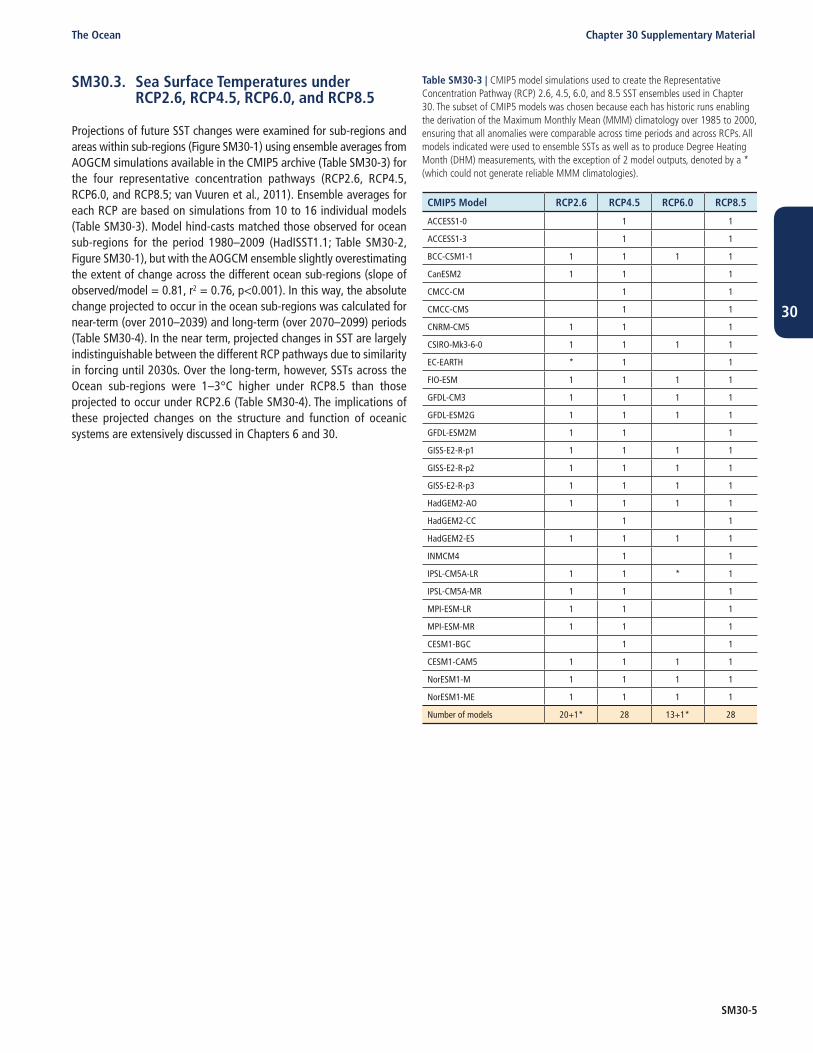
SM30.3. Sea Surface Temperatures underRCP2.6, RCP4.5, RCP6.0, and RCP8.5

Projections of future SST changes were examined for sub-regions andareas within sub-regions (Figure SM30-1) using ensemble averages fromAOGCM simulations available in the CMIP5 archive (Table SM30-3) forthe four representative concentration pathways (RCP2.6, RCP4.5,RCP6.0, and RCP8.5; van Vuuren et al., 2011). Ensemble averages foreach RCP are based on simulations from 10 to 16 individual models(Table SM30-3). Model hind-casts matched those observed for oceansub-regions for the period 1980–2009 (HadISST1.1; Table SM30-2,Figure SM30-1), but with the AOGCM ensemble slightly overestimatingthe extent of change across the different ocean sub-regions (slope ofobserved/model = 0.81, r2 = 0.76, p<0.001). In this way, the absolutechange projected to occur in the ocean sub-regions was calculated fornear-term (over 2010–2039) and long-term (over 2070–2099) periods(Table SM30-4). In the near term, projected changes in SST are largelyindistinguishable between the different RCP pathways due to similarityin forcing until 2030s. Over the long-term, however, SSTs across theOcean sub-regions were 1–3°C higher under RCP8.5 than thoseprojected to occur under RCP2.6 (Table SM30-4). The implications ofthese projected changes on the structure and function of oceanicsystems are extensively discussed in Chapters 6 and 30.

CMIP5 Model RCP2.6 RCP4.5 RCP6.0 RCP8.5

ACCESS1-0 1 1

ACCESS1-3 1 1

BCC-CSM1-1 1 1 1 1

CanESM2 1 1 1

CMCC-CM 1 1

CMCC-CMS 1 1

CNRM-CM5 1 1 1

CSIRO-Mk3-6-0 1 1 1 1

EC-EARTH * 1 1

FIO-ESM 1 1 1 1

GFDL-CM3 1 1 1 1

GFDL-ESM2G 1 1 1 1

GFDL-ESM2M 1 1 1

GISS-E2-R-p1 1 1 1 1

GISS-E2-R-p2 1 1 1 1

GISS-E2-R-p3 1 1 1 1

HadGEM2-AO 1 1 1 1

HadGEM2-CC 1 1

HadGEM2-ES 1 1 1 1

INMCM4 1 1

IPSL-CM5A-LR 1 1 * 1

IPSL-CM5A-MR 1 1 1

MPI-ESM-LR 1 1 1

MPI-ESM-MR 1 1 1

CESM1-BGC 1 1

CESM1-CAM5 1 1 1 1

NorESM1-M 1 1 1 1

NorESM1-ME 1 1 1 1

Number of models 20+1* 28 13+1* 28

Table SM30-3 | CMIP5 model simulations used to create the Representative Concentration Pathway (RCP) 2.6, 4.5, 6.0, and 8.5 SST ensembles used in Chapter 30. The subset of CMIP5 models was chosen because each has historic runs enabling the derivation of the Maximum Monthly Mean (MMM) climatology over 1985 to 2000, ensuring that all anomalies were comparable across time periods and across RCPs. All models indicated were used to ensemble SSTs as well as to produce Degree Heating Month (DHM) measurements, with the exception of 2 model outputs, denoted by a * (which could not generate reliable MMM climatologies).

SM30-6


30

Continued next page

Table SM30-4 | Projected changes in sea surface temperature (SST ºC) over the next 90 years for ocean sub-regions (Figure SM30-1) from AOGCM model simulations from the Coupled Model Intercomparison Project Phase 5 (CMIP5, http://cmip-pcmdi.llnl.gov/cmip5/). Simulations were available for four Representative Concentration Pathways (RCPs): RCP2.6, RCP4.5, RCP6.0, and RCP8.5. The CMIP5 models used in this analysis are listed in Table SM30-3. For each ocean sub-region, a linear regression was fi tted to all 1x1 degree monthly SST data extracted from the models for each of three periods; 2010 – 2039, 2040 – 2069, and 2070 – 2099. The average change in SST was calculated by multiplying the slope of each linear regression by 360 (months) to derive the average change over each successive 30-year period. The table is divided into two sections: “Near-term (2010 – 2039)” (the average change in SST over the next 30 years) and “Long-term (2010 – 2099)” (the total change over 2010 – 2099, which was calculated by adding the average change of the three 30-year periods from 2010 to 2099). This is a simplifi ed method to account for slight non-linearity in SST change over the 90-year period.

Sub-region AreaNear-term (2010–2039) Long-term (2010–2099) RCP8.5

minus RCP2.6RCP2.6 RCP4.5 RCP6.0 RCP8.5 RCP2.6 RCP4.5 RCP6.0 RCP8.5

1. High Latitude Spring Bloom Systems (HLSBS)

Indian Ocean 0.13 0.29 0.18 0.41 – 0.16 0.49 0.83 2.01 2.17

North Atlantic Ocean 0.31 0.56 0.52 0.65 0.54 1.54 1.95 3.02 2.48

South Atlantic Ocean 0.17 0.36 0.20 0.45 – 0.09 0.67 0.88 2.26 2.36

North Pacifi c Ocean (west) 0.79 0.96 0.91 1.17 1.46 2.47 3.07 4.84 3.38

North Pacifi c Ocean (east) 0.79 0.81 0.93 1.06 1.31 2.17 2.96 4.39 3.08

North Pacifi c Ocean 0.79 0.88 0.92 1.11 1.35 2.31 3.01 4.60 3.25

South Pacifi c Ocean (west) 0.17 0.40 0.25 0.50 – 0.16 0.63 0.85 2.37 2.53

South Pacifi c Ocean (east) 0.12 0.23 0.13 0.35 – 0.09 0.45 0.75 1.70 1.79

South Pacifi c Ocean 0.14 0.28 0.17 0.40 – 0.12 0.51 0.78 1.91 2.03

2. Equatorial Upwelling Systems (EUS)

Atlantic Equatorial Upwelling 0.43 0.58 0.49 0.81 0.46 1.19 1.61 3.03 2.56

Pacifi c Equatorial Upwelling 0.35 0.55 0.54 0.77 0.43 1.22 1.75 3.01 2.57

3. Semi-Enclosed Seas (SES)

Arabian Gulf 0.82 0.97 0.89 1.20 1.30 2.39 2.96 4.26 2.96

Baltic Sea 0.73 1.24 0.92 1.20 1.32 2.74 3.06 4.37 3.05

Black Sea 0.74 1.01 0.86 1.24 1.37 2.61 3.16 4.19 2.82

Mediterranean Sea 0.72 0.87 0.84 1.09 1.37 2.10 2.82 4.08 2.70

Red Sea 0.56 0.72 0.71 0.93 0.88 1.65 2.39 3.45 2.57

4. Coastal Boundary Systems (CBS)

Atlantic Ocean (west) 0.34 0.40 0.45 0.62 0.23 0.81 1.33 2.44 2.21

Caribbean Sea/Gulf of Mexico 0.50 0.67 0.64 0.85 0.74 1.53 1.97 3.23 2.49

Indian Ocean (west) 0.46 0.59 0.56 0.85 0.63 1.39 1.95 3.32 2.69

Indian Ocean (east) 0.34 0.57 0.46 0.69 0.38 1.22 1.59 2.80 2.42

Indian Ocean (east), Southeast Asia, Pacifi c Ocean (west)

0.48 0.66 0.57 0.82 0.66 1.47 1.89 3.12 2.46

5. Eastern Boundary Upwelling Ecosystems (EBUE)

Benguela Current 0.30 0.43 0.45 0.71 0.07 0.70 1.41 2.52 2.45

California Current 0.62 0.71 0.84 0.93 1.02 1.86 2.46 3.51 2.49

Canary Current 0.55 0.62 0.58 0.82 0.97 1.30 1.83 3.18 2.21

Humboldt Current 0.22 0.43 0.34 0.60 0.11 0.91 1.22 2.58 2.47

6. Sub-Tropical Gyres (STG)

Indian Ocean 0.30 0.44 0.37 0.63 0.19 0.89 1.35 2.62 2.43

North Atlantic Ocean 0.49 0.66 0.60 0.85 0.87 1.62 1.98 3.30 2.43

South Atlantic Ocean 0.25 0.33 0.33 0.55 0.03 0.58 1.03 2.20 2.18

North Pacifi c Ocean (west) 0.54 0.70 0.64 0.90 0.84 1.62 2.08 3.39 2.55

North Pacifi c Ocean (east) 0.56 0.66 0.71 0.91 0.90 1.56 1.50 3.44 2.54


South Pacifi c Ocean (west) 0.31 0.44 0.34 0.62 0.12 0.88 1.19 2.56 2.44

South Pacifi c Ocean (east) 0.17 0.27 0.21 0.45 – 0.03 0.52 0.89 1.90 1.93

South Pacifi c Ocean 0.20 0.31 0.24 0.49 0.00 0.60 0.96 2.05 2.05

Coral Reef Provinces; see Figure 30-4b

Caribbean Sea/Gulf of Mexico 0.48 0.64 0.61 0.83 0.68 1.43 1.87 3.14 2.46

Coral Triangle and Southeast Asia 0.42 0.61 0.52 0.76 0.58 1.35 1.75 2.95 2.37

Indian Ocean (east) 0.32 0.56 0.46 0.67 0.37 1.18 1.59 2.76 2.40

Indian Ocean (west) 0.39 0.51 0.50 0.77 0.43 1.18 1.71 2.97 2.54

Pacifi c Ocean (east) 0.46 0.64 0.64 0.83 0.63 1.44 1.99 3.23 2.60

Pacifi c Ocean (west) 0.35 0.48 0.40 0.68 0.30 1.02 1.39 2.66 2.35

SM30-7


30

Sub-region AreaNear-term (2010–2039) Long-term (2010–2099) RCP8.5

minus RCP2.6RCP2.6 RCP4.5 RCP6.0 RCP8.5 RCP2.6 RCP4.5 RCP6.0 RCP8.5

Basin Scale North Atlantic Ocean 0.37 0.60 0.55 0.72 0.66 1.57 1.96 3.12 2.46

South Atlantic Ocean 0.21 0.35 0.27 0.51 – 0.03 0.62 0.76 2.23 2.26

Atlantic Ocean 0.32 0.50 0.44 0.65 0.38 1.17 1.54 2.78 2.40


South Pacifi c Ocean 0.18 0.30 0.21 0.45 – 0.04 0.56 0.89 2.00 2.04

Pacifi c Ocean 0.41 0.54 0.51 0.73 0.52 1.23 1.70 2.97 2.45

Indian Ocean 0.30 0.44 0.37 0.63 0.19 0.89 1.35 2.62 2.43

Table SM30-4 (continued)

SM30-8


30

SM30.4. Changes to Surface pH and AragoniteSaturation State under DifferentConcentrations of Atmospheric CO2

The relative changes in pH and the aragonite saturation state ofseawater varies in concert with increases in the partial pressure of CO2

above the ocean. Observations of ocean chemistry (Doney et al., 2009;Feely et al., 2009) are highly consistent with models of the carbonatechemistry of the upper ocean (Caldeira and Wickett, 2003). Notably,high latitude areas, as well as regions where upwelling is dominant,show naturally lower pH and aragonite saturation states. These regionsare expected to reach critical levels in terms of pH and aragonitesaturation sooner than lower latitudes and non-upwelling regions(Section 30.3.2.2).

SM30-9


30

(a) Ocean pH as a function of atmospheric CO2 concentration

Ocean pH

280ppm

450ppm

394ppm

800ppm

280ppm

450ppm

394ppm

800ppm

(b) Aragonite saturation state

7.6 7.8 8.0 8.2 8.3

Aragonite saturation state

0.00 3.132.50 5.00

Figure SM30-2 | The carbonate chemistry of the Ocean under current different atmospheric concentration s of CO2. 280ppm represents pre-industrial and 394ppm present-day levels (WGI Annex II). (a) Surface pH and (b) Aragonite saturation state of the Ocean simulated by the University of Victoria Earth System Model. The fields of pH and aragonite saturation state are calculated from the model output of dissolved inorganic carbon concentration, alkalinity concentration, temperature, and salinity, together with the chemistry routine from the OCMIP-3 project (http://www.ipsl.jussieu.fr/OCMIP/phase3).

SM30-10


30

SM30.5. Projections of Changes to Sea SurfaceTemperatures (RCP2.6 and RCP8.5)for Different Regions that have CoralReefs

Warm-water coral reefs throughout the world (but particularly in CBS,SES, and STG; Figure SM30-1) are rapidly declining as result of localperturbations (i.e., coastal pollution, overexploitation) and climatechange (high confidence; Sections 30.5.3-4, 30.5.6). Reef-buildingcorals, which are responsible for building the carbonate framework ofcoral reefs, are sensitive to both elevated sea temperatures as well asreduced pH and carbonate concentrations (high confidence; Section6.3.2; Boxes CC-CR, CC-OA). Continued increases in sea temperaturewill increase the incidence of impacts such as mass coral bleaching andmortality (virtually certain), with the CMIP5 ensemble projecting theirreversible degradation of coral reefs from most sites globally by 2050(very likely; Section 30.5; Figure 30-10; Box CC-CR). Investigating past,present, and future sea temperatures in six major coral reef areas (Figure30-4b) reveals that future sea temperatures will exceed establishedthresholds of coral bleaching and mortality around the middle to latepart of this century (Figure SM30-3).

References

Caldeira, K. and M. E. Wickett, 2003: Oceanography: anthropogenic carbon andocean pH. Nature, 425(6956), 365-365.

Doney, S.C., V.J. Fabry, R.A. Feely, and J.A. Kleypas, 2009: Ocean acidification: theother CO2 problem. Annual Review of Marine Science, 1, 169-192.

Feely, R.A., S.C. Doney, and S.R. Cooley, 2009: Ocean acidification: present conditionsand future changes in a high-CO2 world. Oceanography, 22(4), 36-47.

Field, C.B., M.J. Behrenfeld, J.T. Randerson, and P. Falkowski, 1998: Primary productionof the biosphere: integrating terrestrial and oceanic components. Science, 281,237-240.

Rayner, N.A., D.E. Parker, E.B. Horton, C.K. Folland, L.V. Alexander, D.P. Rowell, E.C.Kent, and A. Kaplan, 2003: Global analyses of sea surface temperature, sea ice,and night marine air temperature since the late nineteenth century. Journal ofGeophysical Research, 108(D14), 4407.

van Vuuren, D.P., J. Edmonds, M. Kainuma, K. Riahi, A. Thomson, K. Hibbard, G.C.Hurtt, T. Kram, V. Krey, J.-F. Lamarque, T. Masui, M. Meinshausen, N. Nakicenovic,S.J. Smith, and S.K. Rose, 2011: The representative concentration pathways: anoverview. Climatic Change, 109, 5-31.

SM30-11


30

Historical

Natural RCP2.6

RCP8.5

OverlapOverlap

Caribbean & Gulf of Mexico Coral Triangle & Southeast Asia

Western Indian Ocean Western Pacific Ocean

Eastern Indian Ocean

Observed

Eastern Pacific Ocean

°C 5

3

2

1

0

–21900 1950 2000 2050 2100

–1

4

°C 5

3

2

1

0

–21900 1950 2000 2050 2100

–1

4

°C 5

3

2

1

0

–21900 1950 2000 2050 2100

–1

4

°C 5

3

2

1

0

–21900 1950 2000 2050 2100

–1

4

°C 5

3

2

1

0

–21900 1950 2000 2050 2100

–1

4

°C 5

3

2

1

0

–21900 1950 2000 2050 2100

–1

4

Figure SM30-3 | Past and future sea surface temperatures (SST) in six major coral reef provinces and locations (Figure 30-4b) under historic, un-forced (natural), RCP2.6 and RCP8.5 scenarios from CMIP5 ensembles (Table SM30-3). Observed and simulated variations in past and projected future annual average SST over various sites where coral reefs are prominent ecosystems (locations shown in Figure 30-4b). The black line shows estimates from HadISST1.1 [Rayner et al., 2003] reconstructed historical SST dataset. Shading denotes the 5–95 percentile range of climate model simulations driven with ‘historical’ changes in anthropogenic and natural drivers (62 simulations), historical changes in ‘natural’ drivers only (25), the RCP4.5 emissions scenario (62), and the RCP8.5 (62). Data are anomalies from the 1986–2006 average of the HadISST1.1 data (for the HadISST1.q time series) or of the corresponding historical all- forcing simulations. Further details are given in Box 21.1, 21.3.

the ocean - on-line supplementary material - ipcc.ch · supplementary material ... entire regions...

Documents