Online Investors: Do the Slow Die First?

Brad M. Barber* Graduate School of Management, UC-Davis

bmbarber@ucdavis.edu www.gsm.ucdavis.edu/~bmbarber

Terrance Odean* Haas School of Business, UC-Berkeley

odean@ucdavis.edu faculty.haas.berkeley.edu/odean

This Draft: October 2001

∗ We appreciate the comments of an anonymous reviewer, Franklin Allen, Randy Beatty, Ken French, Ravi

Jagannathan, John Heaton, Andrew Metrick, Cesare Robotti, Chuck Schnitzlein, Michael Vetsuypens, and seminar participants at the Berkeley Program in Finance (November 1999), National Bureau of Economic Research Behavioral Finance Group (December 1999), the European Finance Association meetings, the Maryland Finance Symposium, the Review of Financial Studies Behavior Finance Conference, the Western Finance Association meetings (June 2000), Princeton, the Rodney L White Conference on Household Financial Decision-Making (March 2001), the Securities and Exchange Commission, Southern Methodist University, UC-Berkeley, the University of Iowa, the University of Utah, and Yale University. Michael Foster provided valuable research assistance. All errors are our own.

Abstract We analyze 1,607 investors who switch from phone-based to online trading during the

1990s. Those who switch to online trading perform well prior to going online, beating the

market by more than two percent annually. After going online, they trade more actively,

more speculatively, and less profitably than before -- lagging the market by more than

three percent annually. Reductions in market frictions (lower trading costs, improved

execution speed, and greater ease of access) do not explain these findings.

Overconfidence – augmented by self-attribution bias and the illusions of knowledge and

control – can explain the increase in trading and reduction in performance of online

investors.

1

[The giant] tortoise lives longer than any other animal. Collier’s Encyclopedia

“Online trading is like the old west,” warns Fidelity Investments. “The slow die

first.” “Trading at home? Slow can kill you,” echoes a provider of internet connections.

“If your broker's so great, how come he still has to work?” asks E*TRADE. Another

E*TRADE ad notes online investing is: “A cinch. A snap. A piece of cake.” “I'm

managing my portfolio better than my broker ever did,” claims a middle-aged woman

(Datek Online). In Ameritrade's “Momma's Gotta Trade,” two suburban moms return

from jogging. Straight to her computer, a few clicks and a sale later, one declares “I think

I just made about $1,700!” Her kids cheer, while her friend laments, “I have mutual

funds.” And then there is Discover Brokerage's online trading tow-truck driver. He picks

up a snobbish executive who spots a postcard on the dashboard and asks “Vacation?”

“That's my home,” says the driver. “Looks more like an island,” says the executive.

“Technically, it's a country,” replies the driver.

These advertisements entice and amuse. They assure the uninitiated that they have

what it takes to trade online; tell them what to expect—sudden wealth; and what will be

expected of them—frequent trades. They also reinforce cognitive biases, which, for the

most part, do not improve investors' welfare.

In general, when the price of a product declines, the quantity demanded of the

product increases, as does consumer welfare. This has been the case, for example, with

personal computers over the last decade. While consumers are always better off paying

less for the same goods, there are situations where the increased demand associated with

lower prices is a questionable boon to individuals and a clear loss to society. An extreme

example is increased consumption of cigarettes due to price cuts or greater ease of access.

In recent years, there has been an explosion in online trading that is likely to

continue. Forrester Research, Inc. (Punishill (1999)) projects “that by 2003, 9.7 million

U.S. households will manage more than $3 trillion on-line—nearly 19 percent of total

retail investment assets—in 20.4 million on-line accounts.” The growth in online trading

2

has been accompanied by a drop in trading commissions.1 Lower commissions, greater

ease of access, and speedier trade executions constitute reductions in market frictions.

Such reductions of friction generally improve markets. However, while these changes can

obviously benefit investors, to the extent that they encourage excessive, speculative

trading, this benefit is attenuated.

In this paper, we provide a description of those who switch from phone-based to

online trading. Multivariate analyses document that young men who are active traders

with high incomes and a preference for investing in small growth stocks with high market

risk are more likely to switch to online trading. We find that those who switch to online

trading experience unusually strong performance prior to going online, beating the

market by more than two percent annually.

We also examine the change in trading behavior that takes place when investors

go online. In doing so, we test the theory that overconfidence leads to excessive trading.

Consistent with that theory, we find that, after going online, investors trade more

actively, more speculatively, and less profitably than before. It is difficult to reconcile

these results with rational behavior.

Human beings are overconfident about their abilities, their knowledge, and their

future prospects. Odean (1998a) shows that overconfident investors trade more than

rational investors and that doing so lowers their average utilities, since overconfident

investors trade too aggressively when they receive information about the value of a

security. Greater overconfidence leads to greater trading and to lower average utility.2

1 Credit Suisse First Boston Technology Group (Burnham and Earle (1999)) reports a 70% drop in the

average commission charged by the top ten online trading firms from first quarter 1996 to fourth quarter 1997, though commissions have remained largely unchanged from fourth quarter 1997 through first quarter 1999.

2 Kyle and Wang (1997) and Benos (1998) show that under particular circumstances when both a rational

insider and overconfident insider trade strategically and simultaneously with a market maker, the overconfident insider may earn greater profits than the rational insider. The overconfident insider earns greater profits by “precommitting” to trading aggressively. For this result to hold, traders must have sufficient resources and risk tolerance to trade up to the Cournot equilibrium, trade on correlated information, and know each other’s overconfidence. It is unlikely that these models describe individual

3

Due to several cognitive biases, in addition to selection bias, the investors we observe

switching from phone based trading to online trading are likely to have been

overconfident about their ability to profit from trading online. The reduced costs and

increased ease of online trading is most appealing to active traders. Thus, particularly in

these early years, online trading may have attracted more overconfident, more active

investors. However, this selection bias alone will not cause online investors to perform

worse after they commence online trading. (However, it is possible that investors whose

confidence has recently increased are particularly likely to anticipate more active future

trading and to therefore avail themselves of the benefits of trading online.)

We posit that online investors become more overconfident once online for three

reasons: the self-attribution bias, an illusion of knowledge, and an illusion of control.

People tend to attribute their successes to their own abilities, even when such attribution

is unwarranted (self-attribution bias). Thus, recent investment success is likely to foster

overconfidence in one’s stock picking abilities. We find that those who switched from

phone-based to online trading did so after a period of unusually strong performance,

which may have engendered greater overconfidence. People also become more

overconfident when given more information on which to base a forecast (the illusion of

knowledge) and they behave as if their personal involvement can influence the outcome

of chance events (the illusion of control). Online investors have access to vast quantities

of information, generally manage their own portfolios, and trade at the click of a mouse.

These aspects of online trading foster greater overconfidence. And greater

overconfidence leads to elevated trading and poor performance -- precisely the portrait of

the online investors that we study.

The paper proceeds as follows. We motivate our test of overconfidence in Section

I. In Section II, we describe the data and methods. We present our main results in

Section III. We discuss our results in Section IV and conclude in Section V.

investors, who have limited resources, trade asynchronously, and do not know the overconfidence levels of those with whom they trade.

4

1. A Test of Overconfidence

1.1 Overconfidence and Trading on Financial Markets Studies of the calibration of subjective probabilities find that people tend to

overestimate the precision of their knowledge (Alpert and Raiffa (1982); Fischhoff,

Slovic and Lichtenstein (1977); see Lichtenstein, Fischhoff, and Phillips (1982) for a

review of the calibration literature). Such overconfidence has been observed in many

professional fields. Clinical psychologists (Oskamp (1965)), physicians and nurses,

(Christensen-Szalanski and Bushyhead (1981); Baumann, Deber, and Thompson (1991)),

investment bankers (Staël von Holstein (1972)), engineers (Kidd (1970)), entrepreneurs

(Cooper, Woo, and Dunkelberg (1988)), lawyers (Wagenaar and Keren (1986)),

negotiators (Neale and Bazerman (1990)), and managers (Russo and Schoemaker (1992))

have all been observed to exhibit overconfidence in their judgments. (For further

discussion, see Lichtenstein, Fischhoff, and Phillips (1982) and Yates (1990).)

Overconfidence is greatest for difficult tasks, for forecasts with low predictability,

and for undertakings lacking fast, clear feedback (Fischhoff, Slovic, and Lichtenstein

(1977); Lichtenstein, Fischhoff, and Phillips (1982); Yates (1990); Griffin and Tversky

(1992)). Selecting common stocks that will outperform the market is a difficult task.

Predictability is low; feedback is noisy. Thus, stock selection is the type of task for which

people are most overconfident.

Survey and experimental evidence supports our contention that investors are

overconfident. Since October 1996, Paine Webber has sponsored 13 separate Gallup

surveys of individual investors. In each of these 13 surveys, on average, investors

expected their own portfolios to beat the market.3 For example, in October 1999,

investors expected their portfolios to return, on average, 15.7 percent over the next twelve

3 In each of these surveys, investors were asked two questions: “What overall rate of return do you expect

to get on your portfolio in the NEXT twelve months,” and “Thinking about the stock market more generally, what overall rate of return do you think the stock market will provide investors during the coming twelve months?” Across the 13 surveys, the average investor expects a return of 15 percent on their own portfolio, while they expect the market to return 13 percent.

5

months, while they expected the market to return 13.3 percent. Moore, Kurtzberg, Fox,

and Bazerman (1999) generate similar results in an investment experiment using 80 MBA

students.

DeBondt and Thaler (1995) note that the high trading volume on organized

exchanges is perhaps the single most embarrassing fact to the standard finance paradigm,

and that the key behavioral factor needed to understand the trading puzzle is

overconfidence. DeLong, Shleifer, Summers, and Waldmann (1991), Kyle and Wang

(1997), Benos (1998), Daniel, Hirshleifer, and Subramanyam (1998, 2001), Odean

(1998a), Gervais and Odean (2000), and Caballé and Sákovics (1998) develop theoretical

models based on the assumption that investors are overconfident. Most of these models

predict that overconfident investors will trade more than rational investors.

In theoretical models overconfident investors overestimate the precision of their

knowledge about the value of a financial security.4 They may also overestimate the

probability that their personal assessments of the security’s value are more accurate than

the assessments of others. Thus overconfident investors believe more strongly in their

own valuations, and concern themselves less about the beliefs of others. This intensifies

differences of opinion. And differences of opinion cause speculative trading (Varian

(1989); Harris and Raviv (1993)). Rational investors only trade and only purchase

information when doing so increases their expected utility (e.g., Grossman and Stiglitz

(1980)). Overconfident investors, on the other hand, lower their expected utility by

trading too much and too speculatively; they hold unrealistic beliefs about how high their

returns will be and how precisely these can be estimated; and they expend too many

resources (e.g., time and money) on investment information (Odean 1998a).5

4 Odean (1998a) points out that overconfidence may result from investors overestimating the precision of

their private signals or, alternatively, overestimating their abilities to correctly interpret public signals. 5 In some models that assume investors are overconfident, the overconfident investors may improve their

welfare by trading aggressively. However, the assumptions required to generate this result are unlikely to apply to individual investors, which is the focus of our empirical investigation (see footnote 2).

6

Barber and Odean (2000) and Odean (1999) test whether investors decrease their

expected utility by trading too much. Using the same data set from which the sample

analyzed here is drawn, Barber and Odean (2000) show that after accounting for trading

costs, individual investors underperform relevant benchmarks. Those who trade the most

realize, by far, the worst performance. This is what the models of overconfident investors

predict. Barber and Odean (2001) show that men, who tend to be more overconfident

than women, trade nearly one and a half times more actively than women and thereby

reduce their net returns more so than do women. With a different data set, Odean (1999)

finds that the securities individual investors buy subsequently underperform those they

sell. When he controls for liquidity demands, tax-loss selling, rebalancing, and changes in

risk-aversion, investors' timing of trades is even worse. This result suggests that not only

are investors too willing to act on too little information, but they are too willing to act

when they are wrong.

The overconfidence models predict that more overconfident investors will trade

more actively and will thereby reduce their net returns. In this paper we argue that

investors in our sample who switch to online trading are likely to have been more

overconfident than the average investor and to have been more overconfident after going

online than before. We test for differences in the turnover and returns of online and phone

based investors and for differences before and after investors go online.

1.2 Online investing and Overconfidence

1.2.1 Self-attribution bias Online investors in our sample outperform the market before going online. People

tend to ascribe their successes to their personal abilities and their failures to bad luck or

the actions of others (Miller and Ross (1975); Langer and Roth (1975)), and self-

enhancing attributions following success are more common than self-protective

attributions following failures (Fiske and Taylor (1991), see also Miller and Ross (1975)).

Gervais and Odean (2000) demonstrate this self-attribution bias will cause successful

investors to grow increasingly overconfident about their general trading prowess. (Daniel,

Hirshleifer, and Subrahmanyam (1998) further argue that the self-attribution bias can

7

intensify overreactions and lead to short-term momentum and long-run reversals in stock

prices.) Investors whose recent successes have increased their overconfidence will trade

more actively and more speculatively. Because they anticipate that the effort of switching

to online trading will be amortized over more trades, these investors are more likely to go

online. If self-attribution induced overconfidence triggers investors to go online, online

investors will tend to be more overconfident than phone based investors and more

overconfident subsequent to going online than in the period before.

1.2.2 The Illusion of Knowledge

When people are given more information on which to base a forecast or

assessment, the accuracy of their forecasts tends to improve much more slowly than their

confidence in the forecasts. While the improved accuracy of forecasts yields better

decisions, additional information can lead to an illusion of knowledge and foster

overconfidence, which leads to biased judgments. In a widely cited study, Oskamp

(1965) documents that pyschologists’ confidence in their clinical decisions increased with

more information, but accuracy did not. Several subsequent studies confirm the illusion

of knowledge (e.g., Hoge (1970); Slovic (1973); Peterson and Pitz (1988)).

Online investors have access to vast quantities of investment data. We posit that

online investors are more likely to access and use these data than investors with

traditional brokerage accounts, thus fostering greater overconfidence for online investors.

Online brokerages often tout their data offerings to customers. Waterhouse Securities, for

example, claims to offer more “free investment research and research information on-line

and in print than any other discount broker” including “Real-time Quotes, Historical

Charts, Real-time News, Portfolio Tracking, S&P Stock Reports, [and] Zack’s Earnings

Estimates.” Data provider eSignal promises investors that “You'll make more, because

you know more.” Indeed, online investors have access to nearly all the same data as

professional money managers, though in most cases, they lack the same training and

experience. Investors may be tempted to believe that so much data confers knowledge.

Yet past data may not predict the future. And even when data does offer insights,

investors may catch only glimmers of these. Individual investors, whose purchases

8

habitually underperform their sales by approximately three percentage points in a year

(Odean (1999)), need more than a glimmer of additional insight to profit from trading.

The tendency of more information to increase trading by increasing

overconfidence may be augmented by cognitive dissonance (Festinger (1957)).

Investors who spend a considerable amount of time (or money) gathering data will

generally believe themselves to be reasonable people. Since a reasonable person would

not spend so much time gathering useless data, investors are motivated to believe that the

data are useful. Furthermore, it would be unreasonable to spend so much time gathering

data on how to trade if one didn’t trade. And so, to resolve cognitive dissonance,

information-gathering investors are disposed to trade.

1.2.3 The Illusion of Control

Langer (1975) and Langer and Roth (1975) find that people behave as if their

personal involvement can influence the outcome of chance events -- an effect they label

the illusion of control. These studies document that overconfidence occurs when factors

ordinarily associated with improved performance in skilled situations are present in

situations at least partly governed by chance. Langer finds that choice, task familiarity,

competition, and active involvement all lead to inflated confidence beliefs. Presson and

Benassi (1996) review 53 experiments on the illusion of control and conclude that

“illusion of control effects have been found across different tasks, in many situations, and

by numerous independent researchers” (p.506).

Of the key attributes that foster an illusion of control (choice, task familiarity,

competition, and active involvement), active involvement is most relevant for online

investors. Online investors place their orders without the intermediation of a telephone

broker. They may feel that such active involvement improves their chances of favorable

outcomes and therefore choose to trade more. Balasubramanian, Konana, and Menon

(1999) study survey results from 832 visitors to an online brokerage house’s website.

9

Survey respondents list “feeling of empowerment” as one of seven basic reasons given

for switching to online trading.6

Advertisements for online brokerages often emphasize the importance of taking

control of one’s investments. Young Suretrade investors boast, “We're not relying on the

government. We're betting on ourselves.” Discover Brokerage states bluntly that online

investing is “about control.” A young woman in an Ameritrade ad proclaims “I don’t

want to just beat the market. I want to wrestle its scrawny little body to the ground and

make it beg for mercy.” Such advertisements reinforce investors’ illusion of control.

In summary, overconfident investors trade more actively and more speculatively.

Excessive trading lowers their returns. Due to selection bias, those who go online

(especially during the early years of online trading) are likely to be more overconfident

than other investors. Because of self-attribution bias, the switch to online trading is likely

to coincide with an increase in overconfidence. Furthermore, the illusion of knowledge

and the illusion of control will lead online investors to become more overconfident once

they are online. Thus online investors will tend to be more overconfident than other

investors and more overconfident after going online than before.

1.2.4 Selection Bias Online trading was a recent innovation during our sample period (1991-1996).

The effort and perceived risks of switching to trading online were probably greater then

than they are today. Overconfidence reduces the perception of risk (Odean (1998a)).

Furthermore, more overconfident investors tend to trade more actively and thus

potentially benefit more from online trading. If overconfident investors exist in financial

markets, it is likely that they were disproportionately represented among early online

investors. Thus, there is a selection bias in our sample of investors that switched to

online trading.

6 The other six reasons are: cost, speed and availability, convenience, easy access to reliable information,

lack of trust in and unsatisfactory experiences with traditional brokers, and investor discomfort when communicating directly with traditional brokers.

10

In summary, we have the following testable hypotheses:

H1. Online investors trade more actively once online.

H2. Online investors trade more actively than phone based investors.

H3. Online investors trade more speculatively once online.

H4. Online investors trade more speculatively than phone based investors.

H5. By trading more, online investors hurt their performance more after going

online than before.

H6. By trading more, online investors hurt their performance more than do

phone based investors.

2 Data and Methods

2.1 The Online and Size-Matched Samples

The primary focus of our analysis is 1,607 investors who switched from phone-

based trading to online trading; we refer to these investors as our online sample. These

investors are identified from 78,000 households with brokerage accounts at a large

discount brokerage firm.7 (For expositional ease, we often refer to households as

investors.) For these households, we have all trades and monthly position statements from

January 1991 through December 1996.8 The trade data document how each trade was

initiated (e.g., by phone or by personal computer). The online sample represents all

households that had a common stock position in each month of our six-year sample

period and initiated their first online (i.e., computer-initiated) trade between January 1992

and December 1995. We require six years of position statements so that we can analyze

changes in household investment behavior subsequent to the advent of online trading.

7 Previous studies of the behavior of individual investors include Lewellen, Lease, and Schlarbaum (1977);

Schlarbaum, Lewellen, and Lease (1978a, 1978b); Odean (1998b, 1999); Barber and Odean (2000a, 2000b); Grinblatt and Keloharju (2001); and Shapira and Venezia (2001). These studies do not analyze online trading.

8 The month-end position statements for this period allow us to calculate returns for February 1991 through

January 1997. Data on trades are from January 1991 through November 1996. See Barber and Odean (2000a) for a detailed description of these data.

11

To understand how the trading and performance of the online sample differs from

other investors, we employ a matched-pair research design. Each online investor is size

matched to the investor whose market value of common stock positions is closest to that

of the online investor; this size matching is done in the month preceding the online

investor’s first online trade. As is the case for the online sample, the matched investor

must have a common stock position in each month of our six-year sample period and at

least one common stock trade during the six years. However, the size-matched

households differ from the online households in that they made no online trades during

the six years.9

Our size matching works well. The mean value of month-end common stock

positions held by online investors is $135,000, while that for the control sample is

$132,000; median values are $45,400 and $42,700, respectively. Of the 78,000

households from which these samples are drawn, 27,023 have common stock positions in

all months. For these households, the mean (median) value of positions is $62,700

($21,900). Thus, the online investors have larger mean common stock positions than the

sample at large.

We present descriptive statistics for the online and size-matched samples in Table

1. Data on marital status, children, age, and income are from Infobase Inc. as of June

1997. Self-reported data are information supplied to the discount brokerage firm by

accountholders when they opened their accounts. Income is reported within eight ranges,

where the top range is greater than $125,000. We calculate means using the midpoint of

each range and $125,000 for the top range. Equity to Net Worth (%) is the proportion of

the market value of common stock investment at this discount brokerage firm as of

9 In auxiliary analyses, we matched the online sample to households with the most similar gross return in

the 12 months prior to the switch to online traded. Our main results are very similar to those reported later in the paper. Based on this analysis, the self-attribution bias alone cannot explain the increased trading and resulting poor performance of online investors. It may be that the successful investors most prone to self-attribution bias are the ones who, in anticipation of increased trading, go online. But we believe that other factors specific to the online environment, such as the illusion of knowledge and the illusion of control, also contribute to trading increases and poor performance.

12

January 1991 to total self-reported net worth when the household opened its first account

at this brokerage. Those households with a proportion equity to net worth greater than

100% are deleted when calculating means and medians.

Relative to the size-matched investors, online investors are more likely to be

younger men with higher income and net worth. Their common stock investments also

represent a smaller proportion of their total net worth. Online investors also report having

more investment experience than the size-matched investors. For example, 79 percent of

online investors report having good or extensive investment experience, while 68 percent

of the size-matched investors report the same level of experience and 63 percent of all

accounts report similar levels of experience. In section 3, we provide a comprehensive

multivariate analysis of the characteristics of those who switch from phone-based to

online trading.

2.2 Calculation of Trading Costs

For each trade, we estimate the bid-ask spread component of transaction costs for

purchases ( sprb ) and sales ( sprs ) as:

sprPP

sprPP

sdcl

ds

bdcl

db

s

s

b

b

= −FHGIKJ

= − −FHGIKJ

1

1

,

.

and

(1)

Pdclsand Pd

clb

are the reported closing prices from the Center for Research in Security Prices

(CRSP) daily stock return files on the day of a sale and purchase, respectively;

Pdssand Pd

bbare the actual sale and purchase price from our account database.10 Our

estimate of the bid-ask spread component of transaction costs includes any market impact

that might result from a trade. It also includes an intraday return on the day of the trade.

The commission component of transaction costs is calculated as the dollar value of the

10 Kraus and Stoll (1972), Holthausen, Leftwich, and Mayers (1987), Laplante and Muscarella (1997), and

Beebower and Priest (1980) use closing prices either before or following a transaction to estimate effective spreads and market impact. See Keim and Madhavan (1998) for a review of different approaches to calculating transactions costs.

13

commission paid scaled by the total principal value of the transaction, both of which are

reported in our account data.

We present descriptive statistics on the cost of trading for the online and size-

matched samples for trades of more than $1,000 in Table 2. For both online investors and

their-size matched counterparts, commissions and spreads are lower in the online periods,

reflecting a market wide decline in trading costs. For online investors average round-trip

commissions drop from 3.3 percent to 2.5 percent after they go online, while average

round-trip spreads drop from 1.1 percent to 0.9 percent.11,12 Transaction costs are similar

for the size-matched households.

2.3 Measuring Return Performance

We analyze both the gross performance and net performance (after a reasonable

accounting for commissions, the bid-ask spread, and the market impact of trades). We

estimate the gross monthly return on each common stock investment using the beginning-

of-month position statements from our household data and the CRSP monthly returns

file. In so doing, we make two simplifying assumptions. First, we assume that all

securities are bought or sold on the last day of the month. Thus, we ignore the returns

earned on stocks purchased from the purchase date to the end of the month and include

the returns earned on stocks sold from the sale date to the end of the month. Second, we

ignore intramonth trading (e.g., a purchase on March 6 and a sale of the same security on

March 20), though we do include in our analysis short-term trades that yield a position at

the end of a calendar month. In the current study, an accounting for intramonth trades and

the exact timing of trades would increase the performance of online investors before the

switch to online trading by 10 basis points per year, and decrease the performance of

online investors after the switch by 25 basis points per year.

11 If trades valued at less than $1,000 are included in these calculations, average round-trip commissions

drop from 5.1 percent to 3.4 percent when investors go online. Average round-trip spreads drop from 1.2 percent to 0.9 percent.

12 Since 1996, online commissions have continued to drop while investor trading has increased. To

determine whether investors have benefited from these offsetting trends will require additional research.

14

Consider the common stock portfolio for a particular household. The gross

monthly return on the household's portfolio ( Rhtgr ) is calculated as:

R p Rht it iti

shtgr gr=

=∑

1

, (2)

where pit is the beginning-of-month market value for the holding of stock i by household

h in month t divided by the beginning-of-month market value of all stocks held by

household h , Ritgr is the gross monthly return for stock i, and sht are the number of stocks

held by household h in month t.

For security i in month t, we calculate a monthly return net of transaction costs

( Ritnet ) as:

(3)

where spris and comis are the estimated spread and commission associated with a sale and

sprib and comib are the estimated spread and commission associated with a purchase.13

Because the timing and cost of purchases and sales vary across households, the net return

for security i in month t will vary across households. The net monthly portfolio return for

each household is:

(4)

If only a portion of the beginning-of-month position in stock i was purchased or sold, the

transaction cost is only applied to the portion that was purchased or sold.

13 Had we estimated spreads by dividing transaction prices by closing prices, net returns would be

calculated as: ( ) ( ) ( )( )

1 1 11

11

+ = + −+

−+

R R sprspr

comcomit it

is

ib

is

ib

net gr b gb g .

( ) ( ) ( )( )

1 1 11

11

+ = + −+

−+

R R s p rs p r

c o mc o mit i t

ib

i s

i s

ib

n e t g r b gb g

R p Rht it iti

shtnet net=

=∑

1

.

15

In our analysis of returns, we focus on four monthly return series. The first is the

average experience of online investors before online trading. In each month, we average

the returns of online investors who have not yet begun online trading. Thus, we end up

with a 58-month return series for online investors before switching to online trading

(February 1991 to November 1995 -- December 1995 being the month when the last

online investors begin online trading). The second return series is the average experience

of online investors after switching to online trading. In each month, we average the

returns of online investors who have begun trading online. Thus, we end up with a 60-

month return series for online investors after online trading begins (February 1992 to

January 1997 -- January 1992 being the month when the first online investors begin

online trading). We calculate two analogous return series for the size-matched

investors.14

2.4 Risk-Adjusted Return Performance

We calculate four measures of risk-adjusted performance. In the discussion that

follows, we describe the performance measures for the online sample; there are

analogous calculations for their size-matched counterparts. First, we calculate the mean

monthly market-adjusted abnormal return for online investors by subtracting the return

on a value-weighted index of NYSE/ASE/Nasdaq stocks from the return earned by online

investors.

Second, we calculate an own-benchmark abnormal return for online investors,

which is similar in spirit to that proposed by Grinblatt and Titman (1993) and

Lakonishok, Shleifer, and Vishny (1992). In this abnormal return calculation, the

benchmark for household h is the month t return of the beginning-of-year portfolio held

by household h.15 It represents the return that the household would have earned had it

14 The general tenor of our results are the same if we weight the returns of the online and size-matched

samples by account size rather than equally. 15 When calculating this benchmark, we begin the year on February 1st. We do so because our first monthly

position statements are from the month end of January 1991. If the stocks held by a household at the beginning of the year are missing CRSP returns data during the year, we assume that stock is invested in the remainder of the household’s portfolio.

16

merely held its beginning-of-year portfolio for the entire year. The own-benchmark

abnormal return is the return earned by household h less the own-benchmark return; if the

household did not trade during the year, the own-benchmark abnormal return would be

zero for all twelve months during the year. In each month, the abnormal returns for all

online investors are averaged yielding a monthly time-series of mean monthly own-

benchmark abnormal returns. Statistical significance is calculated using t-statistics based

on this time-series. The advantage of the own-benchmark abnormal return measure is that

it does not adjust returns according to a particular risk model. No model of risk is

universally accepted; furthermore, it may be inappropriate to adjust investors' returns for

stock characteristics that they do not associate with risk. The own-benchmark measure

allows each household to self-select the investment style and risk profile of its benchmark

(i.e., the portfolio it held at the beginning of the year), thus emphasizing the effect trading

has on performance. Own-benchmark returns are our primary measure of the detrimental

effect of overconfidence (and excessive trading) on returns.

Third, we employ the theoretical framework of the Capital Asset Pricing Model

and estimate Jensen’s alpha by regressing the monthly excess return earned by online

investors on the market excess return. For example, to evaluate the gross monthly return

earned by the average online investor ( )ROtgr , we estimate the following monthly time-

series regression:

(5)

where:

Rft = the monthly return on T-Bills,16

Rmt = the monthly return on a value-weighted market index,

αi = the CAPM intercept (Jensen's alpha),

βi = the market beta, and

εit = the regression error term.

16 The return on T-bills is from Stocks, Bonds, Bills, and Inflation, 1997 Yearbook, Ibbotson Associates,

Chicago, IL.

RO R R Rt ft i i mt ft itgr ,− = + − +d i d iα β ε

17

The subscript i denotes parameter estimates and error terms from regression i, where we

estimate four regressions for online investors and four for the size-matched control

sample: one each for the gross and net performance before online trading and one each

for the gross and net performance after online trading.

Fourth, we employ an intercept test using the three-factor model developed by

Fama and French (1993). For example, to evaluate the performance of the average online

investor, we estimate the following monthly time-series regression:

(6)

where SMBt is the return on a value-weighted portfolio of small stocks minus the return

on a value-weighted portfolio of big stocks and HMLt is the return on a value-weighted

portfolio of high book-to-market stocks minus the return on a value-weighted portfolio of

low book-to-market stocks.17 The regression yields parameter estimates of

α βj j j js h, , , and . The error term in the regression is denoted by ε jt . The subscript j

denotes parameter estimates and error terms from regression j, where we again estimate

four regressions for the online sample and four for the control sample.18

Fama and French (1993) argue that the risk of common stock investments can be

parsimoniously summarized as risk related to the market, firm size, and a firm’s book-to-

market ratio. We measure these three risk exposures using the coefficient estimates on

the market excess return ( )R Rmt ft− , the size zero-investment portfolio (SMBt), and the

book-to-market zero-investment portfolio (HMLt) from the three-factor regressions.

Portfolios with above-average market risk have betas greater than one, βj > 1. Portfolios

17 The construction of these portfolios is discussed in detail in Fama and French (1993). We thank Kenneth

French for providing us with these data. 18 Lyon, Barber, and Tsai (1999) document that intercept tests using the three-factor model are well

specified in random samples and samples of large or small firms. Thus, the Fama-French intercept tests employed here account well for the small stock tilt of individual investors.

RO R R R s SMB h HMLt ft j j mt ft j t j t jtgr ,− = + − + + +d i d iα β ε

18

with a tilt toward small (value) stocks relative to a value-weighted market index have size

(book-to-market) coefficients greater than zero, sj > 0 (hj > 0).

We suspect there is little quibble with interpreting the coefficient on the market

excess return (βj) as a risk factor. Interpreting the coefficient estimates on the size and

the book-to-market zero-investment portfolios is more controversial. For the purposes of

this investigation, we are interested in measuring risk as perceived by individual

investors. As such, it is our casual observation that investors view common stock

investment in small firms as riskier than that in large firms. Furthermore, theory supports

the link between firm size and returns (Berk (1995)). Thus, we would willingly accept a

stronger tilt toward small stocks as evidence that a particular group of investors is

pursuing a strategy that they perceive as riskier. It is less clear to us whether investors

believe a tilt towards high book-to-market stocks (which tend to be ugly, financially

distressed, firms) or towards low book-to-market stocks (which tend to be high-growth

firms) is perceived as riskier by investors. Daniel and Titman (1997) provide evidence

that book-to-market effects are attributable to firm characteristics, rather than covariance

with factor risks, while Davis, Fama, and French (2000) provide contrary evidence.

Daniel, Hirshleifer, and Subrahmanyam (2001) argue that overconfidence itself can lead

to a positive relation between book-to-market and returns. As such, we interpret the

coefficient estimates on the book-to-market zero-investment portfolio with a bit more

trepidation. Nonetheless, our primary results are unaffected if we exclude HMLt from the

time-series regressions.

3 Who goes online?

The multivariate analyses presented in this section provide a profile of those who

go online. Young men who are active traders with high incomes and no children are more

likely to switch to online trading. Those who switch also have higher levels of self-

reported investment experience and a preference for investing in small growth stocks

with high market risk. We also document that those who switch to online trading

experience unusually strong performance prior to going online.

19

These conclusions are based on a pooled time-series cross-sectional logistic

regression from January 1992 through December 1995. All households with available

data and six years of common stock positions (from January 1991 through December

1996) are included in the regression. The dependent variable for the regression is a

dummy variable that takes on a value of one in the month that a household begins online

trading and a zero otherwise. Households that go online are excluded from the sample

after going online.19

The independent variables in the regressions fall into three broad categories:

demographic characteristics, investor characteristics, and self-reported data.

Demographic characteristics include gender, marital status, presence of children in the

household, age, and income. The effect of gender, marital status, and the presence of

children on the probability of going online are measured with dummy variables that take

on a value of one for women, single investors, and households with children,

respectively. Age is measured in years. Income is reported within eight ranges, where the

top range is greater than $125,000. When estimating the logistic regression, we use the

midpoint of each income range and include a dummy variable that takes on a value of one

for households with income greater than $125,000.

Investor characteristics include account size, market-adjusted return, turnover,

and preferences for market risk, small firms, and value stocks. Account size is measured

as the log of the dollar value of common stock investments in January 1991, the start of

our sample period. Market-adjusted return for month t is the mean gross monthly return

on the household’s common stock portfolio less a value-weighted market index from

month t-12 to t-1. Monthly turnover for month t is one half the sum of purchases and

sales divided by the sum of month-end positions from month t-12 to t-1; when estimating

the regression we use the log of one plus monthly turnover. Market-adjusted returns and

monthly turnover are the only variables that vary from one month to the next for a

19 We estimate the logistic regression by pooling over time so that we can more precisely measure turnover

and return performance in the period preceding a switch to online trading. When we estimate the regression using households, rather than household months, as the unit of observation, the results for the remaining independent variables are qualitatively similar.

20

particular household. Preferences for market risk, small firms, and value stocks are

inferred from Fama-French three-factor model, where a separate regression is estimated

for each household.20

Self-reported data include net worth, the ratio of equity to net worth, and

investment experience. Net worth is the log of self-reported net worth. Equity to net

worth is the proportion of the market value of common stock investment at this discount

brokerage firm as of January 1991 to total self-reported net worth when the household

opened its first account at this brokerage. Three dummy variables, which take on a value

of one for those reporting limited, good, or extensive investment experience

(respectively), are used to measure the effect of experience. We suspect that while self-

reported experience is largely based on objective criteria such as the number of years or

the amount of money that one has invested, people vary in how they interpret these

criteria. We also suspect that, ceteris paribus, the more overconfident investors are likely

to overstate their experience.

The results of this analysis are presented in Table 3. Self reported data are

available for only about one-third of the total sample. Consequently, we estimate two

regressions -- one that includes only independent variables for demographics and investor

characteristics and one that includes independent variables for demographics, investor

characteristics, and self-reported data. The results of the first logistic regression are

presented in columns two and three of the table. Of the variables considered, only

marital status has no significant effect on the probability of going online. The remaining

coefficient estimates are all reliably nonzero (p < .10). The results of the regressions

requiring self-reported data are present in the last two columns of the table. Of the self-

reported data, experience has a significant effect of the probability of going online; those

with greater self-reported investment experience (perhaps because they are more

20 Using the full sample six-year sample period to estimate household investment preferences assumes that

preferences of online households do not change significantly after going online. In Section 4.6, we document that there is not a significant change in investment style once households begin trading online.

21

overconfident) are more likely to make the switch. The remaining independent variables

have coefficient estimates that are generally consistent with those in the regression that

excludes self-reported data, though the statistical significance of some coefficients is

weakened -- likely a result of the smaller sample size.

4 Results

In this section, we test and confirm our hypotheses about the trading activity and

return performance of online investors. Our four principal results are that those who

switch from phone-based trading to online trading:

• experience unusually strong performance prior to going online,

• accelerate their trading after going online,

• trade more speculatively after going online, and

• experience subpar performance (as a result of the accelerated trading) after going

online.

We consider each of these results in turn.

4.1 Performance before the Switch

Before the switch to online trading, the average online investor outperforms both

the market and the average size-matched investor. The returns both groups earned before

the switch are presented in columns two through four of Table 4. Before switching the

gross returns of the average online investor beat the market by 35 basis points a month

(4.2 percent annually, p = 0.09), and outpaced the average size-matched investor by 18

basis points a month (2.2 percent annually, p = 0.02). Even after netting out trading costs

the average online investor still beat the market by 20 basis points a month (2.4 percent

annually, not statistically significant) and outpaced the net returns of the average sized-

matched investor by 14 basis points a month (1.7 percent annually, p = 0.08).21

21 Before going online, the gross performance of online traders is positive for all of our return measures

except the own-benchmark measure which is essentially zero (-0.014, t = -0.55). Thus the superior returns earned before going online were due primarily to the portfolios these investors held at the beginning of our evaluation period, not to the trades they made during this period.

22

We argue that the strong performance of online investors before the switch

fostered greater overconfidence. Thus, our primary interest in this analysis is to identify

how investors perceived their own performance before the switch to online trading. We

believe market-adjusted returns are the most relevant measure of performance during this

period. To the extent individual investors evaluate their own performance against a

benchmark, it is likely that they use the market return. The average online investor

comfortably beat the market before the switch to online trading. Many investors likely

gauge the success of their investments on nominal, rather than market-adjusted returns.

Those that do so may attribute their high returns to their own abilities rather than market

returns (about 18 percent annually during the six-year sample period). Regardless of the

performance measure employed, the average online investor earned higher returns than

the average size-matched investor prior to the switch.

4.2 Turnover

We begin our analysis of turnover by calculating aggregate turnover for online

and size-matched investors in event time, where we define month 0 as the month of the

first online trade. For example, for online investors we calculate aggregate turnover in

event time as one half the total value of purchases and sales by all online investors in an

event month (the numerator) divided by the sum of month-end position statements for

that event month (the denominator).

We present annualized turnover (monthly turnover times twelve) in event-time in

Figure 1. In the two years prior to the switch to online trading, annualized turnover for

the online investors averaged about 70 percent, while that for the size-matched investors

averaged about 50 percent. In the month after the switch to online trading (month 1),

annualized turnover of the online investors surges to 120 percent. While a temporary

surge in trading activity is not surprising, a full two years after the switch to online

trading annualized turnover is still 90 percent for the online investors -- well above their

turnover rate in the period prior to the switch. There is no such change in the observed

turnover of the size-matched investors.

23

To more formally test whether the increase in turnover for online investors is

reliably greater than that for their size-matched counterparts, we calculate turnover

separately for each investor. Monthly turnover for each household is one half the total

value of purchases and sales, now summed over time, (the numerator) divided by the sum

of month-end position statements over time (the denominator). For each online and size-

matched household, we calculate two turnover measures -- one before and one after

online trading. (The month of the first online trade is excluded from both calculations.)

The annual turnover (monthly turnover times twelve) of online investors and their size-

matched counterparts are presented in Table 5, Panel A. Both before and after the switch,

online investors trade more actively than their size-matched counterparts.

After switching online, investors trade much more actively than before. Their

average annual turnover increases from 73.7 to 95.5 percent (p < 0.01), thus confirming

hypothesis H1. While online investors trade more actively than their size-matched

counterparts both before and after the switch, the difference in average turnover is much

greater after the switch. This confirms hypothesis H2. In the post-switch period, the

average turnover of online investors is nearly double that of their size-matched

counterparts (95.5 percent versus 48.2 percent, p < 0.01).22

Though the switch to online trading is associated with greater trading activity, it is

possible that those who switched to online trading would have traded more actively

regardless of the whether they were online or not. Though we are unable to dismiss this

possibility within the context of our study, Choi, Laibson, and Metrick (2000) provide

corroborating evidence that it is the online environment that spawns greater trading. They

document that at companies which adopted web-based interfaces for plan participants

during the 1990s, turnover in 401(k) accounts increased by 50 percent; there was no such

increase in trading activity for firms without web-based access.

22 There is also an increase in the turnover of the median online household after the switch to online

trading, though it is much smaller than the increase in average turnover (1.4 percent, p<0.10). Twenty-five percent of the online households increase their turnover by 35 percent or more; Ten percent of the online households increase their turnover by 109 percent or more. Thus, most households increase their trading activity, but some increase their trading dramatically.

24

4.3 Speculative Trading

An investor may trade common stocks for many reasons. An investor with a

bonus to invest or a large bill to pay may buy or sell for liquidity reasons. If one security

in his portfolio appreciates considerably, he may rebalance to restore diversification to

his portfolio (by selling part of his holding in that security and buying others). He may

sell to capture a tax loss. Or he may trade to speculate by selling one stock from his

portfolio and buying another in an effort to improve his performance.

To examine how speculative trading changes when investors go online, we screen

out most trades that may have been motivated by liquidity needs, a desire to rebalance, or

tax-losses. We screen liquidity sales by considering only sales for which a new purchase

follows within three weeks (fifteen trading days) of the sale; most investors who need to

raise cash for less than three weeks have lower cost alternatives available than trading

stocks (e.g., credit cards). We screen rebalancing sales by considering only sales of the

complete holding of a position. We eliminate tax-loss sales by considering only sales for

a profit. In short, we consider all profitable sales of complete positions that are followed

by a purchase within three weeks as speculative and all purchases made within three

weeks of a speculative sale as speculative. It is unlikely that we identify all (or even

most) speculative trades, but those trades that meet our screens are very likely to be

speculative.

As reported in Table 5, Panel B, speculative turnover nearly doubles when

investors go online (from 16.4 to 30.2 percent), confirming hypothesis H3. Even with our

conservative classification, speculative trading accounts for 60 percent of the increase in

turnover for the average online investor. Both before and after the switch, online

investors trade more speculatively than their size-matched counterparts. This confirms

hypothesis H4.

Do investors trade more speculatively because they are better able to identify and

execute profitable speculative trades after going online? To answer this question, we

compare the returns earned by stocks subsequent to speculative purchases and to

25

speculative sales. In each month, we construct a portfolio comprised of those stocks

purchased speculatively in the preceding three months. The daily returns on this portfolio

are calculated as:

RT R

T

pbi

pbipb

i

n

ipb

i

nτ

τ τ

τ

= =

=

∑

∑1

1

(7)

where Tipb

τ is the aggregate value of all speculative purchases in security i from day τ-63

through τ-1 and Ripbτ is the gross daily return of stock i on day τ. We compound the daily

returns within a month, which yields a time-series of monthly returns for four portfolios:

one for speculative purchases before going online ( Rtpb ), one for speculative purchases

after going online ( Rtpa ) one for speculative sales before going online ( Rt

sb ), and one for

speculative sales after going online ( Rtsa ).

Before going online, the stocks online investors buy speculatively outperform

those that they sell speculatively by 59 basis points per month (p=0.08).23 After going

online, the stocks online investors buy speculatively underperform those that they sell

speculatively by 27 basis points per month, though the underperformance is not reliably

different from zero (p=0.29). The difference in the relative performance of purchases and

sales before and after going online is significant (p = 0.10).24 Though the speculative

trades of online investors performed well prior to switching online, these profits would

not be sufficient to cover average round-trip transaction costs of four percent (see Table

2). Furthermore, online investors were unable to sustain their solid gross performance.

23 This t-statistic is calculated as: tR R

R Rtpb

tsb

tpb

tsb

=−

−c hc hσ / 56

.

24 If we look at all trades, not just speculative trades, the stocks online investors buy before going online

outperform those they sell by an insignificant 29 basis points a month (p = 0.15). After going online their buys underperform their sells by a significant 31 basis points a month (p=0.05).

26

4.4 Performance After the Switch

The returns earned by online investors after the switch to online trading and those

of their size-matched counterparts are presented in columns five through seven of Table

4. After the switch to online trading, online investors perform poorly. The gross returns

of online investors underperform the market by 9 basis points a month (not statistically

significant), while their net returns underperform by an economically large 29 basis

points a month (3.5 percent annually, p=0.13). Net own benchmark returns indicate that

after the switch, online investors lose 30 basis points a month (3.6 percent annually)

through their trading activities, while the size match group lose only 12 basis points (1.4

percent annually); both shortfalls and their difference are significant at the 1 percent

level, confirming hypothesis H6.

4.5 Changes in Performance

In this section, we formally test whether the changes in performance -- from

before to after online trading -- are significant. To do so, we compare the returns earned

by online investors who have not yet gone online to those earned, during the same

months, by online investors who have already begun trading online. For our online

sample, the first online trading begins in January 1992 and the last households commence

online trading in December 1995. Thus, we can calculate the before-after return series

for 46 months -- February 1992 to November 1995. The results of this analysis are

presented in Table 6. (Returns in Tables 4 and 6 differ because their observation periods

differ.)

Using any of our return measures, the gross and net returns of online investors

who have already switched to online trading are less than those of who have not yet made

the switch. For example, the average net raw return of online investors who have

commenced trading online is 36 basis points a month lower than that of online investors

who have not yet made the switch (4.3 percent annually, p < 0.01). After going online

net own-benchmark returns are 15 basis points a month lower (p < 0.01), confirming

hypothesis H5. Without equivocation, we can conclude that there is a dramatic erosion in

the performance of online investors after they switch to online trading. This erosion is

27

due to the combination of better than average (gross) performance before the switch and

inferior performance (both gross and net) afterwards.25

4.6 The Investment Style of Online Investors

It is natural to wonder whether the investment style of online investors differs

from other investors. The answer is yes and no. Yes, since relative to the size-matched

sample, online investors tilt their investments toward small growth stocks with higher

market risk.26 No, since the tilt toward small growth stocks with high market risk is

apparent both before and after online trading. There is some evidence that online

investors increase their exposure to small growth stocks after going online (the test

statistic is 1.36 for the coefficient estimate on the SMBt and -2.11 for HMLt). However,

there is a similar style change for the size-matched control group; there are no significant

differences in these changes between the online investors and the control group. At face

value, it does not appear that the switch from phone-based to online investing is

accompanied by a significant change in the style of stocks investors own.

5 Discussion

We find that those who switch from phone-based trading to online trading:

• experience unusually strong performance prior to the switch,

• accelerate their trading after going online,

• trade more speculatively after going online, and

25 An analogous analysis for the size-matched households yields differences in net performance (after

online less before online) ranging from 8 basis points (own-benchmark abnormal return) to -14 basis points (market-adjusted returns). The change in net performance of the online sample (after online less before online) less the change in performance for the size-matched households range from -21 basis points (Fama-French alpha) to -26 basis points (own-benchmark abnormal return); all of the differences between the online and size-matched samples are statistically significant at less than the 5 percent level (two-tailed).

26 These conclusions are based on the coefficient loadings and associated test statistics from the time-series

regressions that employ the Fama-French three-factor model. The online investors also have a preference for stocks with poor recent return performance relative to their size-matched counterparts. This inference is drawn by adding a zero-investment portfolio that is long stocks that have performed well recently and short stocks that have performed poorly (see, Carhart (1997)). None of our conclusions regarding performance are altered by the inclusion of this price momentum variable. We thank Mark Carhart for providing us with these return data.

28

• experience subpar performance (as a result of the accelerated trading) after going

online.

The strong performance prior to going online is consistent with self-attribution

bias. Investors with unusually good returns are likely to have taken too much credit for

their success and grown more overconfident about their stock picking abilities.

Overconfident investors were more likely to go online and once online the illusion of

control and the illusion of knowledge further increased their overconfidence.

Overconfidence led them to trade active and active trading caused subpar performance.

For overconfident investors, the greater effort of initiating trades by phone or,

more recently, the higher commissions associated with phone trades, may serve as

unintended barriers to excessive trading. When these market frictions are reduced, the

disutility of increased speculative losses may offset utility gains from lower trading effort

and cost.

While our results are consistent with the overconfidence model of trading and

confirmed all of our hypotheses based that model, other explanations warrant

consideration.

Investors may be trading more after they go online simply because lower trading

costs make more trades potentially profitable. If so, online trading should lead to

improved performance, which it does not.

Some investors may anticipate unusual liquidity needs and switch online in

hopes of facilitating liquidity driven purchases or sales more easily. This could explain

temporary increases in trading after going online. It does not account for higher

permanent levels of online trading, unless traders experience permanent shifts in their

liquidity based trading needs. Furthermore, changes in liquidity based trading do not

explain observed increases in speculative trading after investors go online.

29

It is conceivable that, through greater speed of execution, online trading allows

investors to make profitable trades that would not have otherwise been available. If so,

online trading should lead to improved performance, which it does not.

Investors may trade more when they go online simply because of greater ease of

access. For rational investors this implies that there were potentially profitable trades that

the investors declined to make before going online because the expected profits did not

warrant the effort of calling a broker. Due to the greater ease of trading online, these

investors now make such trades. Such investors must have placed a high cost on the

effort required to phone their discount broker. While this explanation is consistent with

increased trading after going online, it does not explain subpar performance.

Lower trading costs, liquidity needs, speed of execution, and ease of access do not

explain why rational investors would trade more actively, more speculatively, and less

profitably after going online. A final possibility is that rational investors trade more

actively online simply because online investing is entertaining. We cannot rule out the

possibility that we are observing the actions of fully rational investors who knowingly

trade to their financial detriment simply for fun. We believe it more plausible though that

the investors who find trading most fun are those who are overconfident about their

chances of success. The Gallup survey and experimental evidence (Moore et al., 1999)

cited earlier show that investors expect to beat the market. If investors rationally trade

for entertainment, they will recognize that the price of this entertainment is below-

average performance; overconfident investors will expect to beat the market. For a more

detailed discussion of this issue, see Barber and Odean (2000, 2001).

Another reason why investors trade more actively online may be that they simply

misunderstand trading costs. While the commissions they pay are explicitly reported to

investors, bid-ask spreads are not. Our online traders pay aggregate roundtrip

commissions of about 3.3 percent and bid-ask spreads of about 1.1 percent before going

online. After going online, they pay about 2.5 percent roundtrip commissions and 0.9

percent in spread. Commissions fell faster during this period, and subsequently, than

30

spreads. If investors ignore spreads when assessing their trading costs, they may conclude

that total costs have fallen much faster than is actually the case. This misapprehension

will encourage trade.27

When overconfident investors go online, they are likely to trade more for the

same reasons rational investors would trade more: lower costs, faster executions, easier

access (and entertainment). Unlike rational investors, however, overconfident investors

tend to incorrectly identify profitable speculative trades (Odean, 1999). Therefore

increased trading hurts their performance. Thus overconfidence, coupled with the lure of

cheaper, faster, easier trading, explains increased trading and speculation as well as

impaired performance after investors go online.

6 Conclusion

We analyze the characteristics, trading, and performance of 1,607 investors who

switched from phone-based to online trading between 1992 and 1995. During this period,

young men who were active traders with high incomes and no children were more likely

to switch to online trading. Those who switched also had higher levels of self-reported

investment experience and a preference for investing in small growth stocks with high

market risk.

Investors who went online during the period 1992 through 1995, generally earned

superior returns before switching to online trading. After the switch, they increased their

trading activity, traded more speculatively, and performed subpar. Rational investors

would not do this. Overconfident investors, on the other hand, are inclined to trade

excessively.

27 An additional bias that may encourage some investors to trade online is loss aversion. Kahneman and

Tversky (1979) argue that, when faced with losses, people will accept additional risks in hopes of recovering to the former status quo. While we do not believe that most investors are motivated to go online by loss aversion, some may be. An E*TRADE advertisement reads: “The Tooth Fairy, Santa Claus, Social Security.” The implied failure of social security would be a loss of anticipated welfare for many people. The prospect of such a loss could prompt people to take risks they might not otherwise take. Some might even go so far as to open an E*TRADE account.

31

Several cognitive biases reinforce the overconfidence of online investors.

Investors who earn strong returns before going online are likely to attribute this success

disproportionately to their own investment ability (rather than luck) and become

overconfident. Once online, investors have access to vast quantities of investment data;

these data can foster an illusion of knowledge, which increases overconfidence. Finally,

online investors generally manage their own stock portfolios and execute trades at the

click of a mouse; this fosters an illusion of control, which reinforces overconfidence.

Investors who do not increase their trading clearly benefit from the convenience

and low costs of trading online. But others, who trade more actively online, risk

offsetting per trade savings with greater cumulative costs and speculative losses. This is

the experience of the online investors we study here.

Online brokers encourage investors to trade speculatively and often. Some of their

advertisements reinforce cognitive biases, such as overconfidence. Others create

unrealistic expectations. While rational investors will consider only the relevant

informational content of advertising, SEC Chairman Arthur Levitt worries that many of

us may be unduly influenced by advertisements that “step over the line and border on

irresponsibility.”28

Advertisements compare online trading to the legendary west where the first to

draw prevailed. Investors are led to believe that profitable investment opportunities are

ephemeral events, seized only by the quick and vigilant. Most investors, however, will

benefit from a slow trading, buy-and-hold strategy. Trigger-happy traders are prone to

shooting themselves in the foot.

28 Speech at National Press Club, May 4, 1999, http://www.sec.gov/news/speeches/spch274.htm.

32

References

Alpert, Marc, and Howard Raiffa, 1982, A progress report on the training of probability

assessors, in Daniel Kahneman, Paul Slovic, and Amos Tversky, eds.: Judgment

Under Uncertainty: Heuristics and Biases, (Cambridge University Press,

Cambridge and New York).

Balasubramanian, S., P. Konana, and N. Menon, 1999, Understanding online investors:

An analysis of their investing behavior and attitudes, Working paper, University

of Texas, Austin.

Barber, Brad M., and Terrance Odean, 2000, Trading is hazardous to your wealth: The

common stock investment performance of individual investors, Journal of

Finance, 55, 773-806.

Barber, Brad M., and Terrance Odean, 2001, Boys will be boys: Gender, overconfidence,

and common stock investment, Quarterly Journal of Economics, 116, 261-292.

Baumann, Andrea O., Raisa B. Deber, and Gail G. Thompson, 1991, Overconfidence

among physicians and nurses: The ``Micro-Certainty, Macro-Uncertainty"

Phenomenon, Social Science and Medicine, 32, 167-174.

Beebower, Gilbert, and William Priest, 1980, The tricks of the trade, Journal of Portfolio

Management 6, 36-42.

Benos, Alexandros V., 1998, Aggressiveness and survival of overconfident traders,

Journal of Financial Markets, 1, 353-383.

Berk, Jonathan, 1995, A critique of size related anomalies, Review of Financial Studies,

8, 275-286.

33

Burnham, Bill, and Jamie Earle, 1999, Online Trading Quarterly: 1st Quarter 1999, Credit

Suisse First Boston Corporation, New York, New York.

Caballé, Jordi, and József Sákovics, 1998, Overconfident speculation with imperfect

competition, working paper, Universitat Autònoma de Barcelona, Spain.

Carhart, Mark M., 1997, On persistence in mutual fund performance, Journal of Finance,

52, 57-82.

Christensen-Szalanski, Jay J., and James B. Bushyhead, 1981, Physicians' use of

probabilistic information in a real clinical setting, Journal of Experimental

Psychology: Human Perception and Performance, 7, 928-935.

Choi, James J., David Laibson, and Andrew Metrick, 2000, Does the Internet Increase

Trading? Evidence from Investor Behavior in 401(k) Plans, working paper,

University of Pennsylvania.

Cooper, Arnold C., Carolyn Y. Woo, and William C. Dunkelberg, 1988, Entrepreneurs'

perceived chances for success, Journal of Business Venturing, 3, 97-108.

Daniel, Kent, David Hirshleifer, and Avanidhar Subrahmanyam, 1998, A theory of

overconfidence, self-attribution, and security market under- and over-reactions,

Journal of Finance, 53, 1839-1886.

Daniel, Kent, David Hirshleifer, and Avanidhar Subrahmanyam, 2001, Overconfidence,

arbitrage, and equilibrium asset pricing, Journal of Finance, 56, 921-965.

Daniel, Kent, and Sheridan Titman, 1997, Evidence on the characteristics of cross

sectional variation in stock returns, Journal of Finance, 52, 1-33.

34

Davis, James L., Eugene F. Fama, and Kenneth R. French, 2000, Characteristics,

covariances, and average returns: 1929 to 1997, Journal of Finance, 55, 389-406.

DeBondt, Werner, and Richard Thaler, 1995, Financial decision-making in markets and

firms: A behavioral perspective. In Finance: Handbooks in Operations Research

and Management Science, vol. 9, eds. Robert A. Jarrow, Vojislav Maksimovic,

and William T. Ziemba, Amersterdam and New York: North-Holland.

De Long, J. Bradford, Andrei Shleifer, Lawrence H. Summers, and Robert J. Waldmann,

1991, The survival of noise traders in financial markets, Journal of Business, 64,

1-19.

Fama, Eugene F., and Kenneth R. French, 1993, Common risk factors in returns on

stocks and bonds, Journal of Financial Economics, 33, 3-56.

Festinger, Leon, 1957, A theory of cognitive dissonance. (Stanford University Press:

Stanford, CA).

Fischhoff, Baruch, Paul Slovic, and Sarah Lichtenstein, 1977, Knowing with certainty:

The appropriateness of extreme confidence, Journal of Experimental Psychology,

3, 552-564.

Gervais, Simon, and Terrance Odean, 2000, Learning to be overconfident, forthcoming,

Review of Financial Studies.

Griffin, Dale, and Amos Tversky, 1992, The weighing of evidence and the determinants

of confidence, Cognitive Psychology, 24, 411-435.

Grinblatt, Mark, and Matti Keloharju, 2001, What makes investors trade?, Journal of

Finance, 56, 589-616.

35

Grinblatt, Mark, and Sheridan Titman, 1993, Performance measurement without

benchmarks: An examination of mutual fund returns, Journal of Business 66, 47-

68.

Grossman, Sanford J. and Joseph E. Stiglitz, 1980, On the impossibility of

informationally efficient markets, American Economic Review, 70, 393-408.

Harris, Milton, and Artur Raviv, 1993, Differences of opinion make a horse race, Review

of Financial Studies 6, 473-506.

Hoge, Robert D., 1970, Confidence in decision as an index of perceived accuracy of

information processing, Psyhonomic Science 18, 351-353.

Holthausen, Robert, Richard Leftwich, and David Mayers, 1987, The effect of large

block transactions of security prices: A cross-sectional analysis, Journal of

Financial Economics 19, 237-267.

Kahneman, Daniel, and Amos Tversky, 1979, Prospect theory: An analysis of decision

under risk, Econometrica, 46, 171-185.

Keim, Donald, and Ananth Madhavan, 1998, The cost of institutional equity trades,

Financial Analysts Journal 54, 50-69.

Kidd, John B., 1970, The utilization of subjective probabilities in production planning,

Acta Psychologica, 34, 338-347.

Kraus, Alan, and Hans Stoll, 1972, Price impacts of block trading on the New York Stock

Exchange, Journal of Finance 27, 569-588.

36

Kyle, Albert S. and Wang, F. Albert, 1997, Speculation duopoly with agreement to

disagree: Can overconfidence survive the market test?, Journal of Finance,

December 52, 2073-2090.

Lakonishok, Josef, Andrei Shleifer, and Robert W. Vishny, 1992, The structure and

performance of the money management industry, in Martin Neil Baily and

Clifford Winston, eds.: Brookings Papers on Economic Activity:

Microeconomics, (Brookings Institution, Washington D.C.).

Langer, Ellen J., 1975, The illusion of control, Journal of Personality and Social

Psychology, 32, 311-328.

Langer, Ellen J., and Jane Roth, 1975, Heads I win, tails it’s chance: The illusion of

control as a function of the sequence of outcomes in a purely chance task, Journal

of Personality and Social Psychology, 32, 951-955.

LaPlante, Michele, and Chris Muscarella, 1997, Do institutions receive comparable

execution in the NYSE and Nasdaq Markets? A transactions study of block

trades, Journal of Financial Economics 45, 97-134.

Lewellen, Wilber G., Ronald C. Lease, Gary G. Schlarbaum, 1977, Patterns of

investment strategy and behavior among individual investors, Journal of

Business, 50, 296-333.

Lichtenstein, Sarah, Baruch Fischhoff, and Lawrence Phillips, 1982, Calibration of

probabilities: The state of the art to 1980. In Judgment Under Uncertainty:

Heuristics and Biases, eds. Daniel Kahneman, Paul Slovic, and Amos Tversky,

Cambridge and New York: Cambridge University Press.

Lyon, John, Brad Barber, and Chih-Ling Tsai, 1999, Holding size while improving power

in tests of long-run abnormal stock returns, Journal of Finance, 54, 165-202.

37

Miller, Dale T., and Michael Ross, 1975, Self-serving biases in attribution of causality:

Fact or fiction? Psychological Bulletin, 82, 213-225.

Moore, Don A., Terri R. Kurtzberg, Craig R. Fox, and Max H. Bazerman, 1999, Positive

illusions and forecasting errors in mutual fund investment decisions,

Organizational Behavior and Human Decision Processes, 79, 95-114.

Neale, Margaret A., and Max H. Bazerman, 1990, Cognition and Rationality in

Negotiation, New York: The Free Press.

Odean, Terrance, 1998a, Volume, volatility, price and profit when all trades are above

average, Journal of Finance, 53, 1887-1934.

Odean, Terrance, 1998b, Are investors reluctant to realize their losses?, Journal of

Finance, 53, 1775-1798.

Odean, Terrance, 1999, Do investors trade too much?, forthcoming, American Economic

Review.

Oskamp, Stuart, 1965, Overconfidence in case-study judgments, Journal of Consulting

Psychology, 29, 261-265.

Peterson, Dane K., and Gordon F. Pitz, 1988, Confidence, uncertainty, and the use of

information, Journal of Experimental Psychology 14, 85-92.

Presson, Paul K., and Victor A. Benassi, 1996, Illusion of control: A meta-analytic

review, Journal of Social Behavior and Personality 11, 493-510.

Punishill, James P., 1999, Net Investing Goes Mainstream, Forrester Research, Inc.,

Cambridge, Massachusetts.

38

Russo, J. Edward, Paul J. H. Schoemaker, 1992, Managing overconfidence, Sloan

Management Review, 33, 7-17.

Schlarbaum, Gary G., Wilbur G. Lewellen, and Ronald C. Lease, 1978a, The common-

stock-portfolio performance record of individual investors: 1964-70, Journal of

Finance 33, 429-441.

Schlarbaum, Gary G., Wilbur G. Lewellen, and Ronald C. Lease, 1978b, Realized returns

on common stock investments: The experience of individual investors, Journal of

Business 51, 299-325.

Shapira, Zur, and Itzhak Venezia, 2001, Patterns of behavior of professionally managed

and independent investors, Journal of Banking and Finance, 25, 1573-1587.

Slovic, Paul, 1973, Behavioral problems of adhering to a decision policy, Working paper,

Oregon Research Institute, Eugene, Oregon.

Staël von Holstein, Carl-Axel S., 1972, Probabilistic forecasting: An experiment related

to the stock market, Organizational Behavior and Human Performance 8, 139-

158.

Varian, Hal R., 1989, Differences of opinion in financial markets, in Courtenay C. Stone,

ed.: Financial Risk: Theory, Evidence and Implications (Proceedings of the

Eleventh Annual Economic Policy conference of the Federal Reserve Bank of St.

Louis, Boston).

Wagenaar, Willem, and Gideon B. Keren, 1986, Does the expert know? The reliability of

predictions and confidence ratings of experts. In Intelligent Decision Support in

Process Environments, eds.: Erik Hollnagel, Giuseppe Mancini, David D. Woods,

eds. Berlin: Springer.

39

Yates, J. Frank, 1990, Judgment and Decision Making, Englewood Cliffs, New Jersey:

Prentice Hall.

40

Appendix A: The Analysis of Trade Timing

In this appendix, we analyze the timing of purchases and sales within a month.

The timing of trades within a month are ignored in our main analysis, since we assume all

purchases and sales are made at month end. The analysis that follows indicates that this

assumption does not materially affect the conclusions presented in the main text. If

anything, this assumption leads us to underestimate the performance of the online sample

prior to the switch, while overestimating their performance after the switch.

For each account with a beginning-of-month position statement in month t, we

identify all purchases in month t-1 and sales in month t. For both purchases and sales, we

calculate the compound return on the stock from the day following the trade to the last

day of the month. For purchases this return is excluded in our main results, while for

sales this return is included. Note that in our main results, we account for the intraday

return on the trade day in our estimate of the bid-ask spread.

The results of our analysis are presented in Table A1. The second (and fourth)

column of this table present aggregate purchase (and sale) turnover calculated as the

aggregate dollar value of purchases (or sales) divided by the aggregate dollar value of

positions held. (This turnover measure is slightly different than that used in the Table 5,

where turnover is calculated for each household and then averaged across households.)

Abnormal returns are calculated for purchases and sales by subtracting the compound

return on the CRSP NYSE/AMEX/Nasdaq value-weighted index. The trade-weighted

mean abnormal returns are presented in columns three (for purchases) and five (for sales)

of Table A1.

First, consider the results for the online sample (Panel A). Prior to the switch to

online trading, from the day following the trade to the end of the month, the stocks that

these investors bought outperformed the value-weighted market index by 14 basis points

per month, while those that they sold outperformed the index by nine basis points. After

the switch to online trading, the stocks that these investors bought underperformed the

value-weighted market index by 33 basis points per month, while those that they sold

41

outperformed the index by 21 basis points. Based on these abnormal returns and our

estimates of turnover, we estimate that the results we present in the main text

underestimate the performance of online investors by 0.23 basis points per month prior to

the switch and overestimate their performance by 3.38 basis points per month after the

switch.

Second, consider the results for the size-matched sample (Panel B). The same

analysis as that outlined in the preceding paragraph indicates that we have overestimated

the performance of the size-matched sample by 0.43 basis points per month prior to the

switch and 2.40 basis points per month after the switch.

Consider how the accounting for the exact timing of trades relates to the return

calculations contained in the main text. In Figure A1, we present an example of a

security that is purchased in month one and sold in month three. A time line for these

transactions is depicted in Figure A1.

In the main text, we calculate the return for this security from t1 to t3. In this

appendix, we calculate the return from timing as the return from tbcl to t1 minus the return

from tscl to ts . Our estimate of the bid-ask spread is the return from ts to ts

cl minus the

return from tb to tbcl . When the return from timing is added to the main calculation and

the spread is subtracted, one gets the (approximate) return from tb to ts , the period in

which the investor held the stock.

42

Table A1

The Gross Abnormal Returns for Stocks Bought and Sold from the Trade Date to the End of the Month

Online households are 1,607 households with 72 consecutive months of common stock positions, no online trades prior to January 1992, and at least one online trade between January 1992 and December 1995. Each size-matched household is the household with the closest account size to the sample firm in the month preceding its first online trade. The matched household must also have 72 consecutive months of common stock positions, no online trades during the 72 months, and at least one trade between January 1992 and December 1995. Purchase turnover is the aggregate value of stocks purchased divided by the aggregate value of stocks held in each month. The purchase abnormal return is calculated by compounding the daily returns on the purchased security from the day following the purchase to the end of the month less the compound return on the value-weighted NYSE/AMEX/Nasdaq market index. Sales turnover and sales abnormal return are analogously calculated. The estimated effect on the monthly abnormal return is purchase turnover times purchase abnormal return minus sale turnover times sale abnormal return.

Sample

Monthly Purchase Turnover

(%)

Purchase Abnormal Return (%)

Monthly

Sale Turnover

(%)

Sale Abnormal Return (%)

Estimated Effect on Monthly

Abnormal Return (%)

Panel A: Online Households Prior to Switch 4.157 0.137 3.774 0.091 0.0023 After Switch 6.260 -0.327 6.311 0.211 -0.0338

Panel B: Size-Matched Households Prior to Switch 3.395 -0.148 3.069 -0.023 -0.0043 After Switch 3.081 -0.807 3.147 -0.029 -0.0240

tb tbcl t1 t2 ts ts

cl t3

Figure

The clo

(sale) m

Close Month 1 Close Month 3

e

Close Month 2

Day of Purchase

A1. Time Line of Returns Calculations. The time o

se on the purchase (sale) day is tbcl ( ts

cl ). The close on

onth is t1 ( t3 ).

Day of Sal

43

f purchase (sale) is tb ( ts ).

the last day of the purchase

44

Appendix B: The Analysis of Intramonth Trades

In this appendix, we analyze the performance of stocks that are bought and then

sold within a calendar month (e.g., purchased on January 3 and sold on January 10).

These intramonth trades are excluded from our main analyses, since those analyses are

based on monthly position statements.

For each account, we identify all purchases followed by a sale within the same

month. In accounting for multiple purchases and sales, we assume that the first securities

purchased are the first sold. We calculate the gross returns on these round-trip

transactions using the CRSP daily return files assuming the security is purchased and sold

at the close of trading on the purchase and sale date, respectively. We calculate the net

returns on these round-trip transactions by subtracting estimates of the bid-ask spread and

commissions as is done in the main text for the case of monthly returns.

In Table B1, we summarize our analysis of the gross and net returns earned on

intramonth trades. In this table, we calculate market-adjusted abnormal returns by

subtracting the daily value-weighted NYSE/AMEX/Nasdaq CRSP market index from the

return earned on each intramonth trade. Both the gross and net abnormal returns in this

table are weighted by the size of each trade, so that we can estimate the aggregate impact

of these intramonth trades on the performance of the online sample and their size-

matched counterparts.

Panel A presents the results for the online sample. Prior to the switch to online

trading, their intramonth trades earn impressive gross abnormal returns of 3.540 percent;

the net abnormal returns are 1.812 percent. Since these intramonth trades represent 0.315

percent of the monthly positions, we estimate that these intramonth trades would improve

the performance of online investors by 0.57 basis points per month (1.812 times

0.00315). After the switch to online trading, intramonth trades would improve the

performance of online investors by 1.26 basis points per month (1.167 time 0.01078).

45

Panel B presents the results for the size-matched sample. Prior to the switch,

intramonth trades improve the performance of the size-matched sample by 0.41 basis

points per month. After the switch, these trades improve their performance by 0.55 basis

points per month. These small improvements in performance for the online sample and

their size-matched counterparts do not materially affect any of the conclusions that we

present in the main text.

In conclusion, we should emphasize that the positive net returns earned on

intramonth trades do not necessarily imply that individual investors have superior short-

term trading ability. If investors have a disposition to sell winning investments and ride

losing investments (as proposed by Shefrin and Statman (1985)), we would expect to

observe positive abnormal returns on short-term round-trip trades.

46

Table B1 The Gross and Net Abnormal Returns earned on Intramonth Trades

Online households are 1,607 households with 72 consecutive months of common stock positions, no online trades prior to January 1992, and at least one online trade between January 1992 and December 1995. Each size-matched household is the household with the closest account size to the sample firm in the month preceding its first online trade. The matched household must also have 72 consecutive months of common stock positions, no online trades during the 72 months, and at least one trade between January 1992 and December 1995. The gross abnormal return on intramonth trades is calculated as the compound return from the day following the purchase to the day of the sale less the compound return on a value-weighted NYSE/AMEX/Nasdaq index. The net abnormal return is the gross abnormal return adjusted for the return earned on the day of the purchase or sale, the bid-ask spread, and the commission cost. The intramonth trades as a percentage of total position value are the average monthly value of intramonth purchases divided by the average monthly value of all stocks held. The estimated effect on monthly abnormal return is the net abnormal return times the intramonth trades as a percentage of total position value.

Sample Mean Trade

Size

Gross Abnormal Return (%)

Net Abnormal Return (%)

Intramonth Trades as a % of Total Position Value

Estimated Change in Monthly

Abnormal Return (%)

Panel A: Online Sample Prior to Switch $13,941 3.540 1.812 0.315 0.0057 After Switch $23,251 2.036 1.167 1.078 0.0126 Panel B: Size-Matched Households Prior to Switch $20,310 2.971 1.447 0.286 0.0041 After Switch $26,562 2.562 1.163 0.470 0.0055

47

Table 1: Demographics of online investors and size-matched investors Online investors are 1,607 investors with 72 consecutive months of common stock positions, no online trades prior to January 1992, and at least one online trade between January 1992 and December 1995. Each size-matched investors is the investor with the closest account size (market value of common stocks held) to the sample firm in the month preceding its first online trade. The matched household must also have 72 consecutive months of common stock positions, no online trades during the 72 months, and at least one trade between January 1992 and December 1995. All accounts are 27,023 accounts with 72 months of common stock positions and no online trades during the 72 months. Data on marital status, children, age, and income are from Infobase Inc. as of June 1997. Self-reported data are information supplied to the discount brokerage firm by accountholders on opening their account. Income is reported within eight ranges, where the top range is greater than $125,000. We calculate means using the midpoint of each range and $125,000 for the top range. Equity to Net Worth (%) is the proportion of the market value of common stock investment at this discount brokerage firm as of January 1991 to total self-reported net worth when the household opened its first account at this brokerage. Those households with a proportion equity to net worth greater than 100% are deleted when calculating means and medians. Infobase data (Panel A) are available for approximately 900 online investors, 900 size-matched investors, and 15,000 of all accounts. Self-reported data (Panel B) are available for 510 online investors, 360 size-matched investors, and 9,500 or all accounts.

Variable Online Size-Matched All Accounts Panel A: Infobase Data

Percentage Men 85.7 79.7 77.2 Percentage Married 76.9 74.9 76.4

Percentage with Children 26.5 25.1 26.6 Mean Age 49.6 53.1 51.6

Median Age 48.0 52.0 50.0 Mean Income ($000) 79.6 74.9 73.9

% with Income > $125,000 12.9 11.1 9.8 Panel B: Self-Reported Data

Net Worth ($000) 90th Percentile 800.0 700.0 525.0 75th Percentile 350.0 300.0 250.0

Median 175.0 125.0 100.0 25th Percentile 87.5 75.0 75.0 10th Percentile 37.5 37.5 37.0

Equity to Net Worth (%) Mean 16.7 19.6 16.4

Median 8.3 11.7 9.0 Investment Experience (%)

None 1.8 3.6 3.8 Limited 19.0 28.7 33.7

Good 57.2 49.3 47.9 Extensive 22.0 18.4 14.6

48

Table 2: Mean Transaction Costs for Trades of Over $1,000 for Online and Size-Matched Households Before and After Online Trading.

Online investors are 1,607 investors with 72 consecutive months of common stock positions, no online trades prior to January 1992, and at least one online trade between January 1992 and December 1995. Each size-matched investors is the investor with the closest account size (market value of common stocks held) to the sample firm in the month preceding its first online trade. The matched household must also have 72 consecutive months of common stock positions, no online trades during the 72 months, and at least one trade between January 1992 and December 1995. Spread is calculated as the transaction price divided by the closing price on the day of the transaction minus one (and then multiplied by minus one for purchases). Commission is calculated as the commission paid divided by the value of the trade. Online Households Size-Matched Households Buys Sells Round-

Trip Buys Sells Round-

Trip

Panel A: Before Online Trading No. of Trades 27,371 19,834 20,739 14,784 Trade Size ($) 9,074 11,414 11,059 14,076 Trade Price ($) 30.85 32.84 32.61 35.25 Spread (%) 0.297 0.836 1.133 0.324 0.761 1.085 Commission (%) 1.697 1.568 3.265 1.637 1.473 3.110

Panel B: After Online Trading No. of Trades 42,296 34,878 17,886 15,001 Trade Size ($) 13,719 16,795 13,780 16,735 Trade Price ($) 31.60 32.53 33.62 34.44 Spread (%) 0.223 0.636 0.859 0.363 0.622 0.985 Commission (%) 1.315 1.192 2.507 1.348 1.246 2.594

49

Table 3: Logistic Regression of the Probability of Switching to Online Trading A pooled time-series, cross-sectional, logistic regression is estimated from January 1992 through December 1995. The dependent variable for the regression is a dummy variable that takes on a value of one in the month that a household begins online trading and a zero otherwise. All households with six years of common stock positions are included in the estimation of the regression. Woman, single, and children are dummy variables that take on a value of one for households headed by a woman, a single person, and households with children. Age is measured in years. Income is reported in eight ranges, where the top range is over $125,000. We also include a dummy variable that takes on a value of one if income is greater than $125,000. Account size is the log of the dollar value of common stock positions held in January 1991. Market-adjusted return in month t is the mean monthly return on the household’s portfolio less a value-weighted market index from month t-12 to t-1. Monthly turnover in month t is one half the sum of purchases and sales divided by the sum of monthly positions from month t-12 to t-1. The regression is estimated using the log of one plus monthly turnover. Market risk, small firm, and value preferences are based on coefficient estimates from the Fama-French three-factor model, which are estimated separately for each household. Net worth is the log of self-reported net worth. Proportion equity to net worth is the value of common stock investments in January 1991 to self-reported net worth. Limited, good, extensive investment experience are dummy variables that take on a value of one for households reporting that level of experience.

50

Table 3, cont’d Number of Households going online

727 377

Observations (Household-Months)

682,121 208,598

Variable Coef. p-value Coef. p-value Intercept -9.197 < 0.001*** -10.209 < 0.001*** Demographics:

woman -0.419 < 0.001*** -0.262 0.082* single -0.087 0.368 -0.018 0.899

children -0.158 0.068* -0.191 0.105* age (years) -0.014 < 0.001*** -0.014 0.005***

income ($000) 0.003 0.081* 0.002 0.258 income > $125 0.050 0.694 0.020 0.906

Investor Characteristics:

Account size (log) 0.165 < 0.001*** 0.082 0.135 Market-adjusted return 4.629 0.002*** 3.106 0.180

Monthly Turnover (log) 0.352 < 0.001*** 0.182 < 0.001*** Market risk preference 0.225 0.012** 0.120 0.357 Small firm preference 0.169 0.002*** 0.133 0.101 Value firm preference -0.256 < 0.001*** -0.192 0.027**

Self-Reported Data:

Net Worth (log) ---- ---- 0.085 0.161 Stock / Net Worth ---- ---- -0.146 0.721

Limited Experience ---- ---- 0.974 0.174 Good Experience ---- ---- 1.503 0.035**

Extensive Experience ---- ---- 1.684 0.019** ***,**,* - significant at the 1, 5, and 10 percent level, respectively.

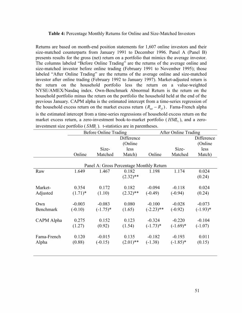
51

Table 4: Percentage Monthly Returns for Online and Size-Matched Investors

Returns are based on month-end position statements for 1,607 online investors and their size-matched counterparts from January 1991 to December 1996. Panel A (Panel B) presents results for the gross (net) return on a portfolio that mimics the average investor. The columns labeled “Before Online Trading” are the returns of the average online and size-matched investor before online trading (February 1991 to November 1995); those labeled “After Online Trading” are the returns of the average online and size-matched investor after online trading (February 1992 to January 1997). Market-adjusted return is the return on the household portfolio less the return on a value-weighted NYSE/AMEX/Nasdaq index. Own-Benchmark Abnormal Return is the return on the household portfolio minus the return on the portfolio the household held at the end of the previous January. CAPM alpha is the estimated intercept from a time-series regression of the household excess return on the market excess return ( )R Rmt ft− . Fama-French alpha is the estimated intercept from a time-series regressions of household excess return on the market excess return, a zero-investment book-to-market portfolio ( HMLt ), and a zero-investment size portfolio ( SMBt ). t-statistics are in parentheses. Before Online Trading After Online Trading

Online

Size-Matched

Difference (Online

less Match)

Online

Size-Matched

Difference (Online

less Match)

Panel A: Gross Percentage Monthly Return

Raw

1.649 1.467 0.182 (2.32)**

1.198 1.174 0.024 (0.24)

Market-Adjusted

0.354 (1.71)*

0.172 (1.10)

0.182 (2.32)**

-0.094 (-0.49)

-0.118 (-0.94)

0.024 (0.24)

Own Benchmark

-0.003 (-0.10)

-0.083 (-1.75)*

0.080 (1.65)

-0.100 (-2.23)**

-0.028 (-0.92)

-0.073 (-1.93)*

CAPM Alpha

0.275 (1.27)

0.152 (0.92)

0.123 (1.54)

-0.324 (-1.73)*

-0.220 (-1.69)*

-0.104 (-1.07)

Fama-French Alpha

0.120 (0.88)

-0.015 (-0.15)

0.135 (2.01)**

-0.182 (-1.38)

-0.193 (-1.85)*

0.011 (0.15)

52

Panel B: Net Percentage Monthly Return

Raw

1.492 1.355 0.137 (1.78)*

1.002

1.082 -0.080 (-0.78)

Market-Adjusted

0.197 (0.97)

0.060 (0.39)

0.137 (1.77)*

-0.291 (-1.52)

-0.211 (-1.69)*

-0.080 (-0.78)

Own Benchmark

-0.160 (-5.83)***

-0.196 (-4.21)***

0.036 (0.76)

-0.297 (-6.50)***

-0.120 (-3.91)***

-0.177 (-4.50)***

CAPM Alpha

0.126 (0.59)

0.044 (0.27)

0.082 (1.03)

-0.519 (-2.77)***

-0.311 (-2.40)**

-0.208 (-2.10)**

Fama-French Alpha

-0.023 (-0.17)

-0.117 (-1.18)

0.094 (1.42)

-0.363 (-2.76)***

-0.280 (-2.67)***

-0.083 (-1.11)

***, **, * significant at the 1, 5, and 10% level, respectively (two-tailed).

53

Table 5: Mean Annual Turnover of Online Households and Size-Matched Households Online households are 1,607 households with 72 consecutive months of common stock positions, no online trades prior to January 1992, and at least one online trade between January 1992 and December 1995. Each size-matched household is the household with the closest account size to the sample firm in the month preceding its first online trade. The matched household must also have 72 consecutive months of common stock positions, no online trades during the 72 months, and at least one trade between January 1992 and December 1995. Monthly turnover for each household is one half the sum of all trades for that household divided by the sum of all month-end positions. Monthly turnover times twelve yields annual turnover. Speculative turnover is calculated using only trades classified as speculative. We define speculative trades as all profitable sales of complete positions that are followed by a purchase within three weeks and all purchases made within three weeks of a speculative sale. Test statistics for the difference in means are based on a two-sample t-statistic assuming unequal variance for the two samples. Before

Online Trading After

Online Trading Change

(After Online less Before Online)

Panel A: Total Turnover

Online Households

73.7 21.8***

95.5

Size-Matched Households

53.2 48.2 -5.0**

Online less Size-Matched

26.8***

20.5*** 47.3***

Panel B: Speculative Turnover Online Households

16.4 30.2 13.8***

Size-Matched Households

11.5 13.9 2.4

Online less Size-Matched

11.4***

4.9*** 16.3***

***, **, * significant at the 1, 5, and 10% level, respectively (two-tailed).

54

Table 6: The Performance of Investors Already Online and Investors Who Have Not Yet Traded Online (but do so before 1997): February 1992 to November 1995

Online households are 1,607 households with 72 consecutive months of common stock positions, no online trades prior to January 1992, and at least one online trade between January 1992 and December 1995. From February 1992 to November 1995, these 1,607 online households are broken into two groups -- those that have already begun online trading (already online) and those that have not yet done so (not yet online). Market-adjusted return is the return on the household portfolio less the return on a value-weighted NYSE/AMEX/Nasdaq index. Own-Benchmark Abnormal Return is the return on the household portfolio minus the return on the portfolio the household held at the end of the previous January. CAPM alpha is the estimated intercept from a time-series regression of the household excess return on the market excess return ( )R Rmt ft− . Fama-French alpha is the estimated intercept from a time-series regressions of household excess return on the market excess return, a zero-investment book-to-market portfolio ( HMLt ), and a zero-investment size portfolio ( SMBt ). t-statistics are in parentheses.

Investors Not Yet Online

Investors Already

Online

Difference (Already Online- Not Yet Online)

Panel A: Gross Percentage Monthly Return

Raw

1.284 0.993 -0.291 (-3.15)***

Market-Adjusted 0.189 (1.08)

-0.104 (-0.52)

-0.291 (-3.15)***

Own Benchmark

0.001 (0.03)

-0.079 (-1.60)

-0.080 (-1.75)*

CAPM Alpha

0.083 (0.46)

-0.240 (-1.19)

-0.323 (-3.32)***

Fama-French

0.145 (0.99)

-0.106 (-0.75)

-0.251 (-2.71)***

55

Panel B: Net Percentage Monthly Return Raw

1.139 0.777 -0.362 (-3.72)***

Market-Adjusted

0.043 (0.25)

-0.319 (-1.60)

-0.362 (-3.72)***

Own Benchmark

-0.144 (-4.60)***

-0.296 (-5.81)***

-0.152 (-3.32)***

CAPM Alpha

-0.057 (-0.32)

-0.453 (-2.23)**

-0.396 (-3.85)***

Fama-French

0.010 (0.07)

-0.301 (-2.11)**

-0.311 (-3.23)***

***, **, * significant at the 1, 5, and 10% level, respectively (two-tailed).

56

Figure 1: Aggregate Turnover for Online and Size-Matched Investors in Event Time (Month 0 = Month of first online trade)

0%

20%

40%

60%

80%

100%

120%

140%

-24 -21 -18 -15 -12 -9 -6 -3 0 3 6 9 12 15 18 21 24

Event Month (0 is month of first online trade)

Annu

aliz

ed T

urno

ver (

%)

Size-Matched

Online

57