the pentagram map: a discrete integrable systemovsienko.perso.math.cnrs.fr/publis/penta.pdf ·...
TRANSCRIPT

Digital Object Identifier (DOI) 10.1007/s00220-010-1075-yCommun. Math. Phys. 299, 409–446 (2010) Communications in
MathematicalPhysics
The Pentagram Map: A Discrete Integrable System
Valentin Ovsienko1, Richard Schwartz2, Serge Tabachnikov3
1 CNRS, Institut Camille Jordan, Université Lyon 1, Villeurbanne Cedex 69622,France. E-mail: [email protected]
2 Department of Mathematics, Brown University, Providence,RI 02912, USA. E-mail: [email protected]
3 Department of Mathematics, Pennsylvania State University, University Park,PA 16802, USA. E-mail: [email protected]
Received: 14 October 2009 / Accepted: 4 February 2010Published online: 24 June 2010 – © Springer-Verlag 2010
Dedicated to the memory of V. Arnold
Abstract: The pentagram map is a projectively natural transformation defined on(twisted) polygons. A twisted polygon is a map from Z into RP
2 that is periodic moduloa projective transformation called the monodromy. We find a Poisson structure on thespace of twisted polygons and show that the pentagram map relative to this Poissonstructure is completely integrable. For certain families of twisted polygons, such asthose we call universally convex, we translate the integrability into a statement aboutthe quasi-periodic motion for the dynamics of the pentagram map. We also explain howthe pentagram map, in the continuous limit, corresponds to the classical Boussinesqequation. The Poisson structure we attach to the pentagram map is a discrete version ofthe first Poisson structure associated with the Boussinesq equation. A research announce-ment of this work appeared in [16].
Contents
1. Introduction . . . . . . . . . . . . . . . . . . . . . . . . . . . . . . . . . . 4102. Proof of the Main Theorem . . . . . . . . . . . . . . . . . . . . . . . . . . 414
2.1 Coordinates for the space . . . . . . . . . . . . . . . . . . . . . . . . . 4142.2 A formula for the map . . . . . . . . . . . . . . . . . . . . . . . . . . . 4152.3 The monodromy invariants . . . . . . . . . . . . . . . . . . . . . . . . 4172.4 Formulas for the invariants . . . . . . . . . . . . . . . . . . . . . . . . 4182.5 The Poisson bracket . . . . . . . . . . . . . . . . . . . . . . . . . . . . 4192.6 The corank of the structure . . . . . . . . . . . . . . . . . . . . . . . . 4212.7 The end of the proof . . . . . . . . . . . . . . . . . . . . . . . . . . . . 421
3. Quasi-periodic Motion . . . . . . . . . . . . . . . . . . . . . . . . . . . . . 4223.1 Universally convex polygons . . . . . . . . . . . . . . . . . . . . . . . 4223.2 The Hilbert perimeter . . . . . . . . . . . . . . . . . . . . . . . . . . . 4233.3 Compactness of the level sets . . . . . . . . . . . . . . . . . . . . . . . 4233.4 Proof of Theorem 2 . . . . . . . . . . . . . . . . . . . . . . . . . . . . 424
410 V. Ovsienko, R. Schwartz, S. Tabachnikov
3.5 Hyperbolic cylinders and tight polygons . . . . . . . . . . . . . . . . . 4253.6 A related theorem . . . . . . . . . . . . . . . . . . . . . . . . . . . . . 426
4. Another Coordinate System in Space Pn . . . . . . . . . . . . . . . . . . . 4274.1 Polygons and difference equations . . . . . . . . . . . . . . . . . . . . 4274.2 Relation between the two coordinate systems . . . . . . . . . . . . . . 4294.3 Two versions of the projective duality . . . . . . . . . . . . . . . . . . 4304.4 Explicit formula for α . . . . . . . . . . . . . . . . . . . . . . . . . . . 4314.5 Recurrent formula for β . . . . . . . . . . . . . . . . . . . . . . . . . . 4324.6 Formulas for the pentagram map . . . . . . . . . . . . . . . . . . . . . 4334.7 The Poisson bracket in the (a, b)-coordinates . . . . . . . . . . . . . . 434
5. Monodromy Invariants in (a, b)-Coordinates . . . . . . . . . . . . . . . . . 4345.1 Monodromy matrices . . . . . . . . . . . . . . . . . . . . . . . . . . . 4355.2 Combinatorics of the monodromy invariants . . . . . . . . . . . . . . . 4365.3 Closed polygons . . . . . . . . . . . . . . . . . . . . . . . . . . . . . . 438
6. Continuous Limit: The Boussinesq Equation . . . . . . . . . . . . . . . . . 4406.1 Non-degenerate curves and differential operators . . . . . . . . . . . . 4406.2 Continuous limit of the pentagram map . . . . . . . . . . . . . . . . . . 4416.3 The constant Poisson structure . . . . . . . . . . . . . . . . . . . . . . 4436.4 Discretization . . . . . . . . . . . . . . . . . . . . . . . . . . . . . . . 444
7. Discussion . . . . . . . . . . . . . . . . . . . . . . . . . . . . . . . . . . . 445
1. Introduction
The notion of integrability is one of the oldest and most fundamental notions in math-ematics. The origins of integrability lie in classical geometry and the development ofthe general theory is always stimulated by the study of concrete integrable systems.The purpose of this paper is to study one particular dynamical system that has a sim-ple and natural geometric meaning and to prove its integrability. Our main tools aremostly geometric: the Poisson structure, first integrals and the corresponding Lagrang-ian foliation. We believe that our result opens doors for further developments involvingother approaches, such as Lax representation, algebraic-geometric and complex analysismethods, Bäcklund transformations; we also expect further generalizations and relationsto other fields of modern mathematics, such as cluster algebras theory.
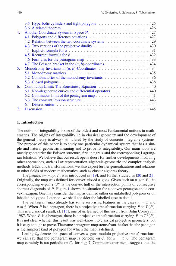
The pentagram map, T , was introduced in [19], and further studied in [20 and 21].Originally, the map was defined for convex closed n-gons. Given such an n-gon P , thecorresponding n-gon T (P) is the convex hull of the intersection points of consecutiveshortest diagonals of P . Figure 1 shows the situation for a convex pentagon and a con-vex hexagon. One may consider the map as defined either on unlabelled polygons or onlabelled polygons. Later on, we shall consider the labelled case in detail.
The pentagram map already has some surprising features in the cases n = 5 andn = 6. When P is a pentagon, there is a projective transformation carrying P to T (P).This is a classical result, cf. [15]; one of us learned of this result from John Conway in1987. When P is a hexagon, there is a projective transformation carrying P to T 2(P).It is not clear whether this result was well-known to classical projective geometers, butit is easy enough to prove. The name pentagram map stems from the fact that the pentagonis the simplest kind of polygon for which the map is defined.
Letting Cn denote the space of convex n-gons modulo projective transformations,we can say that the pentagram map is periodic on Cn for n = 5, 6. The pentagrammap certainly is not periodic on Cn for n ≥ 7. Computer experiments suggest that the

Pentagram Map: A Discrete Integrable System 411
T(P)
P
T(P)
P
Fig. 1. The pentagram map defined on a pentagon and a hexagon
pentagram map on Cn in general displays the kind of quasi-periodic motion one seesin completely integrable systems. Indeed, this was conjectured (somewhat loosely) in[21]. See the remarks following Theorem 1.2 in [21].
It is the purpose of this paper to establish the complete integrability conjectured in[21] and to explain the underlying quasi-periodic motion. However, rather than workwith closed n-gons, we will work with what we call twisted n-gons. A twisted n-gon isa map φ : Z → RP
2 such that that
φ(k + n) = M ◦ φ(k); ∀k.
Here M is some projective automorphism of RP2. We call M the monodromy. For tech-
nical reasons, we require that every 3 consecutive points in the image are in generalposition – i.e., not collinear. When M is the identity, we recover the notion of a closedn-gon. Two twisted n-gons φ1 and φ2 are equivalent if there is some projective transfor-mation � such that � ◦ φ1 = φ2. The two monodromies satisfy M2 = �M1�
−1. LetPn denote the space of twisted n-gons modulo equivalence.
Let us emphasise that the full space of twisted n-gons (rather than the geometricallynatural but more restricted space of closed n-gons) is much more natural in the generalcontext of the integrable systems theory. Indeed, in the “smooth case” it is natural toconsider the full space of linear differential equations; the monodromy then plays anessential rôle in producing the invariants. This viewpoint is adopted by many authors(see [9,14] and references therein) and this is precisely our viewpoint in the discretecase.
The pentagram map is generically defined on Pn . However, the lack of convexitymakes it possible that the pentagram map is not defined on some particular point of Pn ,or that the image of a point in Pn under the pentagram map no longer belongs to Pn .That is, we can lose the 3-in-a-row property that characterizes twisted polygons. We willput coordinates in Pn so that the pentagram map becomes a rational map. At least whenn is not divisible by 3, the space Pn is diffeomorphic to R
2n . When n is divisible by3, the topology of the space is trickier, but nonetheless large open subsets of Pn in thiscase are still diffeomorphic to open subsets of R
2n . (Since our map is only genericallydefined, the fine points of the global topology of Pn are not so significant.)
The action of the pentagram map in Pn was studied extensively in [21]. In that paper,it was shown that for every n this map has a family of invariant functions, the so-calledweighted monodromy invariants. There are exactly 2[n/2]+2 algebraically independent

412 V. Ovsienko, R. Schwartz, S. Tabachnikov
invariants. Here [n/2] denotes the floor of n/2. When n is odd, there are two exceptionalmonodromy functions that are somewhat unlike the rest. When n is even, there are 4such exceptional monodromy functions. We will recall the explicit construction of theseinvariants in the next section, and sketch the proofs of some of their properties. Later onin the paper, we shall give a new treatment of these invariants.
Here is the main result of this paper.
Theorem 1. There exists a Poisson structure on Pn having co-rank 2 when n is odd andco-rank 4 when n is even. The exceptional monodromy functions generically span thenull space of the Poisson structure, and the remaining monodromy invariants Poisson-commute. Finally, the Poisson structure is invariant under the pentagram map.
The exceptional monodromy functions are precisely the Casimir functions for thePoisson structure. The generic level set of the Casimir functions is a smooth sym-plectic manifold. Indeed, as long as we keep all the values of the Casimir functionsnonzero, the corresponding level sets are smooth symplectic manifolds. The remain-ing monodromy invariants, when restricted to the symplectic level sets, define a singularLagrangian foliation. Generically, the dimension of the Lagrangian leaves is precisely thesame as the number of remaining monodromy invariants. This is the classical picture ofArnold-Liouville complete integrability.
As usual in this setting, the complete integrability gives an invariant affine structureto every smooth leaf of the Lagrangian foliation. Relative to this structure, the pentagrammap is a translation. Hence
Corollary 1.1. Suppose that P is a twisted n-gon that lies on a smooth Lagrangian leafand has a periodic orbit under the pentagram map. If P ′ is any twisted n-gon on thesame leaf, then P ′ also has a periodic orbit with the same period, provided that the orbitof P ′ is well-defined.
Remark 1.2. In the result above, one can replace the word periodic with ε-periodic. Bythis we mean that we fix a Euclidean metric on the leaf and measure distances withrespect to this metric.
We shall not analyze the behavior of the pentagram map on Cn . One of the difficultiesin analyzing the space Cn of closed convex polygons modulo projective transformationsis that this space has positive codimension in Pn (codimension 8). We do not know inenough detail how the Lagrangian singular foliation intersects Cn , and so we cannotappeal to the structure that exists on generic leaves. How the monodromy invariantsbehave when restricted to Cn is a subtle and interesting question that we do not yet fullyknow how to answer (see Theorem 4 for a partial result). We hope to tackle the case ofclosed n-gons in a sequel paper.
One geometric setting where our machine works perfectly is the case of universallyconvex n-gons. This is our term for a twisted n-gon whose image in RP
2 is strictlyconvex. The monodromy of a universally convex n-gon is necessarily an element ofPGL3(R) that lifts to a diagonalizable matrix in SL3(R). A universally convex poly-gon essentially follows along one branch of a hyperbola-like curve. Let Un denote thespace of universally convex n-gons, modulo equivalence. We will prove that Un is anopen subset of Pn locally diffeomorphic to R
2n . Further, we will see that the penta-gram map is a self-diffeomorphism of U2n . Finally, we will see that every leaf in theLagrangian foliation intersects Un in a compact set.
Combining these results with our Main Theorem and some elementary differentialtopology, we arrive at the following result.

Pentagram Map: A Discrete Integrable System 413
Theorem 2. Almost every point of Un lies on a smooth torus that has a T -invariantaffine structure. Hence, the orbit of almost every universally convex n-gon undergoesquasi-periodic motion under the pentagram map.
We will prove a variant of Theorem 2 for a different family of twisted n-gons. SeeTheorem 3. The general idea is that certain points of Pn can be interpreted as embedded,homologically nontrivial, locally convex polygons on projective cylinders, and suitablechoices of geometric structure give us the compactness we need for the proof.
Here we place our results in a context. First of all, it seems that there is some con-nection between our work and cluster algebras. On the one hand, the space of twistedpolygons is known as an example of cluster manifold, see [6,7] and discussion in theend of this paper. This implies in particular that Pn is equipped with a canonical Poissonstructure, see [10]. We do not know if the Poisson structure constructed in this papercoincides with the canonical cluster Poisson structure. On the other hand, it was shownin [21] that a certain change of coordinates brings the pentagram map rather closely inline with the octahedral recurrence, which is one of the prime examples in the theory ofcluster algebras, see [11,18,22].
Second of all, there is a close connection between the pentagram map and integrableP.D.E.s. In the last part of this paper we consider the continuous limit of the pentagrammap. We show that this limit is precisely the classical Boussinesq equation which is oneof the best known infinite-dimensional integrable systems. Moreover, we argue that thePoisson bracket constructed in the present paper is a discrete analog of the so-calledfirst Poisson structure of the Boussinesq equation. We remark that a connection to theBoussinesq equation was mentioned in [19], but no derivation was given.
Discrete integrable systems is an actively developing subject, see, e.g., [26] and thebooks [5,23]. The paper [4] discusses a well-known discrete version (but with contin-uous time) of the Boussinesq equation; see [25] (and references therein) for a latticeversion of this equation. See [9] (and references therein) for a general theory of integra-ble difference equations. Let us stress that the r -matrix Poisson brackets considered in[9] are analogous to the second (i.e., the Gelfand-Dickey) Poisson bracket. A geometricinterpretation of all the discrete integrable systems considered in the above referencesis unclear.
In the geometrical setting which is closer to our viewpoint, see [5] for many inter-esting examples. The papers [1,2] considers a discrete integrable system on the spaceof n-gons, different from the pentagram map. The recent paper [13] considers a discreteintegrable systems in the setting of projective differential geometry; some of the formu-las in this paper are close to ours. Finally, we mention [12,14] for discrete and continuousintegrable systems related both to Poisson geometry and projective differential geometryon the projective line.
We turn now to a description of the contents of the paper. Essentially, our plan isto make a bee-line for all our main results, quoting earlier work as much as possible.Then, once the results are all in place, we will consider the situation from another pointof view, proving many of the results quoted in the beginning.
One of the disadvantages of the paper [21] is that many of the calculations are ad hocand done with the help of a computer. Even though the calculations are correct, one is notgiven much insight into where they come from. In this paper, we derive everything in anelementary way, using an analogy between twisted polygons and solutions to periodicordinary differential equations.
One might say that this paper is organized along the lines of first the facts, then thereasons. Accordingly, there is a certain redundancy in our treatment. For instance, we

414 V. Ovsienko, R. Schwartz, S. Tabachnikov
introduce two natural coordinate systems in Pn . In the first coordinate system, whichcomes from [21], most of the formulas are simpler. However, the second coordinatesystem, which is new, serves as a kind of engine that drives all the derivations in bothcoordinate systems; this coordinate system is better for computation of the monodromytoo. Also, we discovered the invariant Poisson structure by thinking about the secondcoordinate system.
In §2 we introduce the first coordinate system, describe the monodromy invariants,and establish the Main Theorem. In §3 we apply the main theorem to universally convexpolygons and other families of twisted polygons. In §4 we introduce the second coor-dinate system. In §4 and 5 we use the second coordinate system to derive many of theresults we simply quoted in §2. Finally, in §6 we use the second coordinate system toderive the continuous limit of the pentagram map.
2. Proof of the Main Theorem
2.1. Coordinates for the space. In this section, we introduce our first coordinate systemon the space of twisted polygons. As we mentioned in the Introduction, a twisted n-gonis a map φ : Z → RP
2 such that
φ(n + k) = M ◦ φ(k) (2.1)
for some projective transformation M and all k. We let vi = φ(i). Thus, the vertices ofour twisted polygon are naturally . . . vi−1, vi , vi+1, . . .. Our standing assumption is thatvi−1, vi , vi+1 are in general position for all i , but sometimes this assumption alone willnot be sufficient for our constructions.
The cross ratio is the most basic invariant in projective geometry. Given four pointst1, t2, t3, t4 ∈ RP
1, the cross-ratio [t1, t2, t3, t4] is their unique projective invariant. Theexplicit formula is as follows. Choose an arbitrary affine parameter, then
[t1, t2, t3, t4] = (t1 − t2) (t3 − t4)
(t1 − t3) (t2 − t4). (2.2)
This expression is independent of the choice of the affine parameter, and is invariantunder the action of PGL(2, R) on RP
1.
Remark 2.1. Many authors define the cross ratio as the multiplicative inverse of the for-mula in Eq. 2.2. Our definition, while perhaps less common, better suits our purposes.
The cross-ratio was used in [21] to define a coordinate system on the space of twistedn-gons. As the reader will see from the definition, the construction requires somewhatmore than 3 points in a row to be in general position. Thus, these coordinates are notentirely defined on our space Pn . However, they are generically defined on our space,and this is sufficient for all our purposes.
The construction is as follows, see Fig. 2. We associate to every vertex vi two num-bers:
xi = [vi−2, vi−1, ((vi−2, vi−1) ∩ (vi , vi+1)) , ((vi−2, vi−1) ∩ (vi+1, vi+2))
],
yi = [((vi−2, vi−1) ∩ (vi+1, vi+2)), ((vi−1, vi ) ∩ (vi+1, vi+2)), vi+1, vi+2], (2.3)
called the left and right corner cross-ratios. We often call our coordinates the cornerinvariants.

Pentagram Map: A Discrete Integrable System 415
i
i+2
vi+1v
i−1
vi−2
v
v
Fig. 2. Points involved in the definition of the invariants
Clearly, the construction is PGL(3, R)-invariant and, in particular, xi+n = xi andyi+n = yi . We therefore obtain a (local) coordinate system that is generically definedon the space Pn . In [21], §4.2, we show how to reconstruct a twisted n-gon from itssequence of invariants. The reconstruction is only canonical up to projective equiva-lence. Thus, an attempt to reconstruct φ from x1, y1, . . . , perhaps would lead to anunequal but equivalent twisted polygon. This does not bother us. The following lemmais nearly obvious.
Lemma 2.2. At generic points, the space Pn is locally diffeomorphic to R2n.
Proof. We can perturb our sequence x1, y1, . . . in any way we like to get a new sequencex ′
1, y′1, . . . . If the perturbation is small, we can reconstruct a new twisted n-gon φ′
that is near φ in the following sense. There is a projective transformation � such thatn-consecutive vertices of �(φ′) are close to the corresponding n consecutive verticesof φ. In fact, if we normalize so that a certain quadruple of consecutive points of �(φ′)match the corresponding points of φ, then the remaining points vary smoothly and alge-braically with the coordinates. The map (x ′
1, y′2, . . . , x ′
n, y′n) → [φ′] (the class of φ′)
gives the local diffeomorphism. Remark 2.3. (i) Later on in the paper, we will introduce new coordinates on all of Pn
and show, with these new coordinates, that Pn is globally diffeomorphic to R2n
when n is not divisible by 3.(ii) The actual lettering we use here to define our coordinates is different from the
lettering used in [21]. Here is the correspondense:
. . . p1, q2, p3, q4 . . . ⇐⇒ . . . , x1, y1, x2, y2, . . . .
2.2. A formula for the map. In this section, we express the pentagram map in the coor-dinates we have introduced in the previous section. To save words later, we say now thatwe will work with generic elements of Pn , so that all constructions are well-defined.Let φ ∈ Pn . Consider the image, T (φ), of φ under the pentagram map. One difficultyin making this definition is that there are two natural choices for labelling T (φ), the left

416 V. Ovsienko, R. Schwartz, S. Tabachnikov
5
2
3
4
5
4
1
right
22
3
4
5
34
1
left
3
Fig. 3. Left and right labelling schemes
choice and the right choice. These choices are shown in Fig. 3. In the picture, the blackdots represent the vertices of φ and the white dots represent the vertices of T (φ). Thelabelling continues in the obvious way.
If one considers the square of the pentagram map, the difficulty in making this choicegoes away. However, for most of our calculations it is convenient for us to arbitrarilychoose right over left and consider the pentagram map itself and not the square of themap. Henceforth, we make this choice.
Lemma 2.4. Suppose the coordinates for φ are x1, y1, . . . then the coordinates for T (φ)
are
T ∗xi = xi1 − xi−1 yi−1
1 − xi+1 yi+1, T ∗yi = yi+1
1 − xi+2 yi+2
1 − xi yi, (2.4)
where T ∗ is the standard pull-back of the (coordinate) functions by the map T .
In [21], Eq. 7, we express the squared pentagram map as the product of two involu-tions on R
2n , and give coordinates. From this equation one can deduce the formula inLemma 2.4 for the pentagram map itself. Alternatively, later in the paper we will give aself-contained proof of Lemma 2.4.
Lemma 2.4 has two corollaries, which we mention here. These corollaries are almostimmediate from the formula. First, there is an interesting scaling symmetry of the pen-tagram map. We have a rescaling operation on R
2n , given by the expression
Rt : (x1, y1, . . . , xn, yn) → (t x1, t−1 y1, . . . , t xn, t−1 yn). (2.5)
Corollary 2.5. The pentagram map commutes with the rescaling operation.
Second, the formula for the pentagram map exhibits rather quickly some invariantsof the pentagram map. When n is odd, define
On =n∏
i=1
xi ; En =n∏
i=1
yi . (2.6)
When n is even, define
On/2 =∏
i even
xi +∏
i odd
xi , En/2 =∏
i even
yi +∏
i odd
yi . (2.7)
The products in this last equation run from 1 to n.

Pentagram Map: A Discrete Integrable System 417
Corollary 2.6. When n is odd, the functions On and En are invariant under the penta-gram map. When n is even, the functions On/2 and En/2 are also invariant under thepentagram map.
These functions are precisely the exceptional invariants we mentioned in the Intro-duction. They turn out to be the Casimirs for our Poisson structure.
2.3. The monodromy invariants. In this section we introduce the invariants of the pen-tagram map that arise in Theorem 1.
The invariants of the pentagram map were defined and studied in [21]. In this sectionwe recall the original definition. Later on in the paper, we shall take a different point ofview and give self-contained derivations of everything we say here.
As above, let φ be a twisted n-gon with invariants x1, y1, . . .. Let M be the monodr-omy of φ. We lift M to an element of GL3(R). By slightly abusing notation, we alsodenote this matrix by M . The two quantities
�1 = trace3(M)
det(M); �2 = trace3(M−1)
det(M−1); (2.8)
enjoy 3 properties.
• �1 and �2 are independent of the lift of M .• �1 and �2 only depend on the conjugacy class of M .• �1 and �2 are rational functions in the corner invariants.
We define
�1 = O2n En�1; �2 = On E2
n�2. (2.9)
In [21] it is shown that �1 and �2 are polynomials in the corner invariants. Since the pen-tagram map preserves the monodromy, and On and En are invariants, the two functions�1 and �2 are also invariants.
We say that a polynomial in the corner invariants has weight k if we have the followingequation:
R∗t (P) = tk P. (2.10)
Here R∗t denotes the natural operation on polynomials defined by the rescaling operation
(2.5). For instance, On has weight n and En has weight −n. In [21] it is shown that
�1 =[n/2]∑
k=1
Ok; �2 =[n/2]∑
k=1
Ek, (2.11)
where Ok has weight k and Ek has weight −k. Since the pentagram map commuteswith the rescaling operation and preserves �1 and �2, it also preserves their “weightedhomogeneous parts”. That is, the functions O1, E1, O2, E2, . . . are also invariants of thepentagram map. These are the monodromy invariants. They are all nontrivial polynomi-als.
Algebraic Independence: In [21], §6, it is shown that the monodromy invariants arealgebraically independent provided that, in the even case, we ignore On/2 and En/2. Wewill not reproduce the proof in this paper, so here we include a brief description of the
418 V. Ovsienko, R. Schwartz, S. Tabachnikov
argument. Since we are mainly trying to give the reader a feel for the argument, we willexplain a variant of the method in [21]. Let f1, . . . , fk be the complete list of invariantswe have described above. Here k = 2[n/2] + 2. If our functions were not algebraicallyindependent, then the gradients ∇ f1, . . . ,∇ fk would never be linearly independent. Torule this out, we just have to establish the linear independence at a single point. Onecan check this at the point (1, ω, . . . , ω2n), where ω is a (4n)th root of unity. The actualmethod in [21] is similar to this, but uses a trick to make the calculation easier. Giventhe formulas for the invariants we present below, this calculation is really just a matterof combinatorics. Perhaps an easier calculation can be made for the point (0, 1, . . . , 1),which also seems to work for all n.
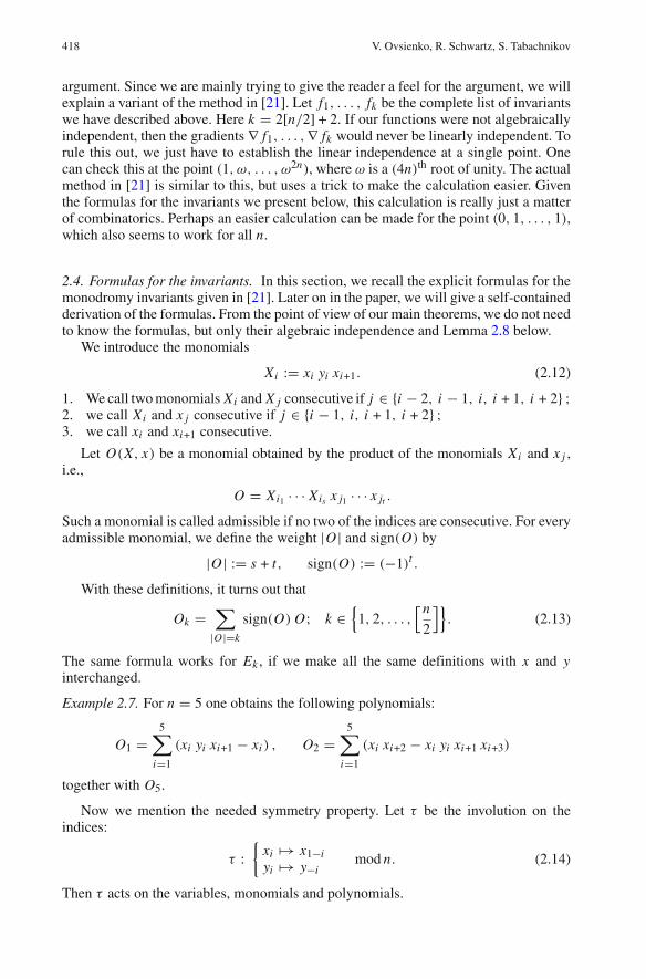
2.4. Formulas for the invariants. In this section, we recall the explicit formulas for themonodromy invariants given in [21]. Later on in the paper, we will give a self-containedderivation of the formulas. From the point of view of our main theorems, we do not needto know the formulas, but only their algebraic independence and Lemma 2.8 below.
We introduce the monomials
Xi := xi yi xi+1. (2.12)
1. We call two monomials Xi and X j consecutive if j ∈ {i − 2, i − 1, i, i + 1, i + 2} ;2. we call Xi and x j consecutive if j ∈ {i − 1, i, i + 1, i + 2} ;3. we call xi and xi+1 consecutive.
Let O(X, x) be a monomial obtained by the product of the monomials Xi and x j ,i.e.,
O = Xi1 · · · Xis x j1 · · · x jt .
Such a monomial is called admissible if no two of the indices are consecutive. For everyadmissible monomial, we define the weight |O| and sign(O) by
|O| := s + t, sign(O) := (−1)t .
With these definitions, it turns out that
Ok =∑
|O|=k
sign(O) O; k ∈{
1, 2, . . . ,[n
2
]}. (2.13)
The same formula works for Ek , if we make all the same definitions with x and yinterchanged.
Example 2.7. For n = 5 one obtains the following polynomials:
O1 =5∑
i=1
(xi yi xi+1 − xi ) , O2 =5∑
i=1
(xi xi+2 − xi yi xi+1 xi+3)
together with O5.
Now we mention the needed symmetry property. Let τ be the involution on theindices:
τ :{
xi �→ x1−iyi �→ y−i
mod n. (2.14)
Then τ acts on the variables, monomials and polynomials.

Pentagram Map: A Discrete Integrable System 419
Lemma 2.8. One has τ(Ok) = Ok.
Proof. τ takes an admissible partition to an admissible one and does not change thenumber of singletons involved.
2.5. The Poisson bracket. In this section, we introduce the Poisson bracket on Pn . LetC∞
n denote the algebra of smooth functions on R2n . A Poisson structure on C∞
n is a map
{ , } : C∞n × C∞
n → C∞n (2.15)
that obeys the following axioms:
1. Antisymmetry: { f, g} = −{g, f }.2. Linearity: {a f1 + f2, g} = a{ f1, g} + { f2, g}.3. Leibniz Identity: { f, g1g2} = g1{ f, g2} + g2{ f, g1}.4. Jacobi Identity: { f1, { f2, f3}} = 0.
Here denotes the cyclic sum.We define the following Poisson bracket on the coordinate functions of R
2n :
{xi , xi±1} = ∓xi xi+1, {yi , yi±1} = ±yi yi+1. (2.16)
All other brackets not explicitly mentioned above vanish. For instance
{xi , y j } = 0; ∀ i, j.
Once we have the definition on the coordinate functions, we use linearity and the Liebnizrule to extend to all rational functions. Though it is not necessary for our purposes, wecan extend to all smooth functions by approximation. Our formula automatically buildsin the anti-symmetry. Finally, for a “homogeneous bracket” as we have defined, it iswell-known (and an easy exercise) to show that the Jacobi identity holds.
Henceforth we refer to the Poisson bracket as the one that we have defined above.Now we come to one of the central results in the paper. This result is our main tool forestablishing the complete integrability and the quasi-periodic motion.
Lemma 2.9. The Poisson bracket is invariant with respect to the pentagram map.
Proof. Let T ∗ denote the action of the pentagram map on rational functions. One hasto prove that for any two functions f and g one has {T ∗( f ), T ∗(g)} = { f, g} and ofcourse it suffices to check this fact for the coordinate functions. We will use the explicitformula (2.4).
To simplify the formulas, we introduce the following notation: ϕi = 1−xi yi . Lemma2.4 then reads:
T ∗(xi ) = xiϕi−1
ϕi+1, T ∗(yi ) = yi+1
ϕi+2
ϕi.
One easily checks that {ϕi , ϕ j } = 0 for all i, j . Next,
{xi , ϕ j } = (δi, j−1 − δi, j+1
)xi x j y j ,
{yi , ϕ j } = (δi, j+1 − δi, j−1
)x j yi y j .
In order to check the T -invariance of the bracket, one has to check that the relationsbetween the functions T ∗(xi ) and T ∗(y j ) are the same as for xi and y j . The first relationto check is: {T ∗(xi ), T ∗(y j )} = 0.

420 V. Ovsienko, R. Schwartz, S. Tabachnikov
Indeed,
{T ∗(xi ), T ∗(y j )
} = {xi , ϕ j+2} y j+1 ϕi−1
ϕi+1 ϕ j− {xi , ϕ j } y j+1 ϕi−1 ϕ j+2
ϕi+1 ϕ2j
−{y j+1, ϕi−1} xi ϕ j+2
ϕi+1 ϕ j+ {y j+1, ϕi+1} xi ϕi−1 ϕ j+2
ϕ2i+1 ϕ j
= (δi, j+1 − δi, j+3
) xi x j+2 y j+2 y j+1 ϕi−1
ϕi+1 ϕ j
− (δi, j−1 − δi, j+1
) xi x j y j y j+1 ϕi−1 ϕ j+2
ϕi+1 ϕ2j
− (δ j+1,i − δ j+1,i−2
) xi−1 y j+1 yi−1 xi ϕ j+2
ϕi+1 ϕ j
+(δ j+1,i+2 − δ j+1,i
) xi+1 y j+1 yi+1 xi ϕi−1 ϕ j+2
ϕ2i+1 ϕ j
= 0,
since the first term cancels with the third and the second with the last one.One then computes {T ∗(xi ), T ∗(x j )} and {T ∗(yi ), T ∗(y j )}, the computations are
similar to the above one and will be omitted. Two functions f and g are said to Poisson commute if { f, g} = 0.
Lemma 2.10. The monodromy invariants Poisson commute.
Proof. Let τ by the involution on the indices defined at the end of the last section. Wehave τ(Ok) = Ok by Lemma 2.8. We make the following claim: For all polynomialsf (x, y) and g(x, y), one has
{τ( f ), τ (g)} = −{ f, g}.
Assuming this claim, we have
{Ok, Ol} = {τ(Ok), τ (Ol)} = −{Ok, Ol},
hence the bracket is zero. The same argument works for {Ek, El} and {Ok, El}.Now we prove our claim. It suffices to check the claim when f and g are monomials
in variables (x, y). In this case, we have: { f, g} = C f g, where C is the sum of ±1,corresponding to “interactions” between factors xi in f and x j in g (resp. yi and y j ).Whenever a factor xi in f interacts with a factor x j in g (say, when j = i + 1, and thecontribution is +1), there will be an interaction of x−i in τ( f ) and x− j in τ(g) yieldingthe opposite sign (in our example, − j = −i − 1, and the contribution is −1). Thisestablishes the claim, and hence the lemma.
A function f is called a Casimir for the Poisson bracket if f Poisson commutes withall other functions. It suffices to check this condition on the coordinate functions. Aneasy calculation yields the following lemma. We omit the details.
Lemma 2.11. The invariants in Eq. 2.7 are Casimir functions for the Poisson bracket.
Pentagram Map: A Discrete Integrable System 421
2.6. The corank of the structure. In this section, we compute the corank of our Poissonbracket on the space of twisted polygons. The corank of a Poisson bracket on a smoothmanifold is the codimension of the generic symplectic leaves. These symplectic leavescan be locally described as levels Fi = const of the Casimir functions. See [27] for thedetails.
For us, the only genericity condition we need is
xi �= 0, y j �= 0; ∀ i, j. (2.17)
Our next result refers to Eq. 2.7.
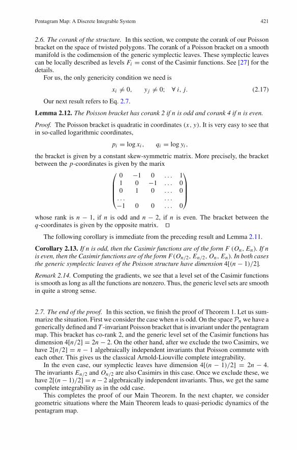
Lemma 2.12. The Poisson bracket has corank 2 if n is odd and corank 4 if n is even.
Proof. The Poisson bracket is quadratic in coordinates (x, y). It is very easy to see thatin so-called logarithmic coordinates,
pi = log xi , qi = log yi ,
the bracket is given by a constant skew-symmetric matrix. More precisely, the bracketbetween the p-coordinates is given by the marix
⎛
⎜⎜⎜⎝
0 −1 0 . . . 11 0 −1 . . . 00 1 0 . . . 0. . . . . .
−1 0 0 . . . 0
⎞
⎟⎟⎟⎠
whose rank is n − 1, if n is odd and n − 2, if n is even. The bracket between theq-coordinates is given by the opposite matrix.
The following corollary is immediate from the preceding result and Lemma 2.11.
Corollary 2.13. If n is odd, then the Casimir functions are of the form F (On, En). If nis even, then the Casimir functions are of the form F(On/2, En/2, On, En). In both casesthe generic symplectic leaves of the Poisson structure have dimension 4[(n − 1)/2].Remark 2.14. Computing the gradients, we see that a level set of the Casimir functionsis smooth as long as all the functions are nonzero. Thus, the generic level sets are smoothin quite a strong sense.
2.7. The end of the proof. In this section, we finish the proof of Theorem 1. Let us sum-marize the situation. First we consider the case when n is odd. On the space Pn we have agenerically defined and T -invariant Poisson bracket that is invariant under the pentagrammap. This bracket has co-rank 2, and the generic level set of the Casimir functions hasdimension 4[n/2] = 2n − 2. On the other hand, after we exclude the two Casimirs, wehave 2[n/2] = n − 1 algebraically independent invariants that Poisson commute witheach other. This gives us the classical Arnold-Liouville complete integrability.
In the even case, our symplectic leaves have dimension 4[(n − 1)/2] = 2n − 4.The invariants En/2 and On/2 are also Casimirs in this case. Once we exclude these, wehave 2[(n − 1)/2] = n − 2 algebraically independent invariants. Thus, we get the samecomplete integrability as in the odd case.
This completes the proof of our Main Theorem. In the next chapter, we considergeometric situations where the Main Theorem leads to quasi-periodic dynamics of thepentagram map.

422 V. Ovsienko, R. Schwartz, S. Tabachnikov
3. Quasi-periodic Motion
In this chapter, we explain some geometric situations where our Main Theorem, anessentially algebraic result, translates into quasi-periodic motion for the dynamics. Theuniversally convex polygons furnish our main example.
3.1. Universally convex polygons. In this section, we define universally convex poly-gons and prove some basic results about them.
We say that a matrix M ∈ SL3(R) is strongly diagonalizable if it has 3 distinctpositive real eigenvalues. Such a matrix represents a projective transformation of RP
2.We also let M denote the action on RP
2. Acting on RP2, the map M fixes 3 distinct
points. These points, corresponding to the eigenvectors, are in general position. M sta-bilizes the 3 lines determined by these points, taken in pairs. The complement of the 3lines is a union of 4 open triangles. Each open triangle is preserved by the projectiveaction. We call these triangles the M-triangles.
Let φ ∈ Pn be a twisted n-gon, with monodromy M . We call φ universally convex if
• M is a strongly diagonalizable matrix.• φ(Z) is contained in one of the M-triangles.• The polygonal arc obtained by connecting consecutive vertices of φ(Z) is convex.
The third condition requires more explanation. In RP2 there are two ways to connect
points by line segments. We require the connection to take place entirely inside theM-triangle that contains φ(Z). This determines the method of connection uniquely.
We normalize so that M preserves the line at infinity and fixes the origin in R2. We
further normalize so that the action on R2 is given by a diagonal matrix with eigenvalues
0 < a < 1 < b. This 2 × 2 diagonal matrix determines M . For convenience, we willusually work with this auxilliary 2 × 2 matrix. We slightly abuse our notation, and alsorefer to this 2 × 2 matrix as M . With our normalization, the M-triangles are the openquadrants in R
2. Finally, we normalize so that φ(Z) is contained in the positive openquadrant.
Lemma 3.1. Un is open in Pn.
Proof. Let φ be a universally convex n-gon and let φ′ be a small perturbation. Let M ′be the monodromy of φ′. If the perturbation is small, then M ′ remains strongly diago-nalizable. We can conjugate so that M ′ is normalized exactly as we have normalized M .
If the perturbation is small, the first n points of φ′(Z) remain in the open positivequadrant, by continuity. But then all points of φ′(Z) remain in the open positive quadrant,by symmetry. This is to say that φ′(Z) is contained in an M ′-triangle.
If the perturbation is small, then φ′(Z) is locally convex at some collection of n con-secutive vertices. But then φ′(Z) is a locally convex polygon, by symmetry. The onlyway that φ(Z) could fail to be convex is that it wraps around on itself. But, the invarianceunder the 2 × 2 hyperbolic matrix precludes this possibility. Hence φ(Z) is convex. Lemma 3.2. Un is invariant under the pentagram map.
Proof. Applying the pentagram map to φ(Z) all at once, we see that the image is againstrictly convex and has the same monodromy.

Pentagram Map: A Discrete Integrable System 423
i
vi+1v
i−1
vi−2
v
vi+2
Fig. 4. Points involved in the definition of the invariants
3.2. The Hilbert perimeter. In this section, we introduce an invariant we call the Hilbertperimeter. This invariant plays a useful role in our proof, given in the next section, thatthe level sets of the monodromy functions in Un are compact.
As a prelude to our proof, we introduce another projective invariant – a function ofthe Casimirs – which we call the Hilbert Perimeter. This invariant is also considered in[19], and for similar purposes.
Referring to Fig. 2, we define
zk = [(vi , vi−2), (vi , vi−1), (vi , vi+1), (vi , vi+2)]. (3.1)
We are taking the cross ratio of the slopes of the 4 lines in Fig. 4.We now define a “new” invariant
H = 1∏n
i=1 zi. (3.2)
Remark 3.3. Some readers will know that one can put a canonical metric inside anyconvex shape, called the Hilbert metric. In case φ is a genuine convex polygon, thequantity − log(zk) measures the Hilbert length of the thick line segment in Fig. 4. (Thereader who does not know what the Hilbert metric is can take this as a definition.) Thenlog(H) is the Hilbert perimeter of T (P) with respect to the Hilbert metric on P . Hencethe name.
Lemma 3.4. H = 1/(On En).
Proof. This is a local calculation, which amounts to showing that zk = xk yk . The bestway to do the calculation is to normalize so that 4 of the points are the vertices of asquare. We omit the details.
3.3. Compactness of the level sets. In this section, we prove that the level sets of themonodromy functions in U are compact.
Let Un(M, H) denote the subset of Un consisting of elements whose monodromy isM and whose Hilbert Perimeter is H . In this section we will prove that Un(M, H) iscompact. For ease of notation, we abbreviate this space by X .
Let φ ∈ X . We normalize so that M is as in Lemma 3.1. We also normalize so thatφ(0) = (1, 1). Then there are numbers (x, y) such that φ(n) = (x, y), independent ofthe choice of φ. We can assume that x > 1 and y < 1. The portion of φ of interestto us, namely φ({0, . . . , n − 1}), lies entirely in the rectangle R whose two opposite
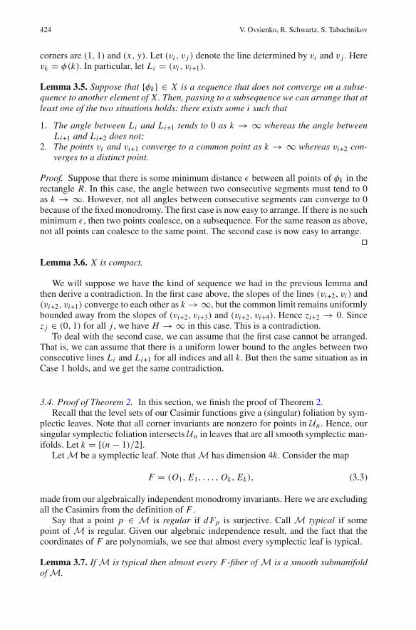
424 V. Ovsienko, R. Schwartz, S. Tabachnikov
corners are (1, 1) and (x, y). Let (vi , v j ) denote the line determined by vi and v j . Herevk = φ(k). In particular, let Li = (vi , vi+1).
Lemma 3.5. Suppose that {φk} ∈ X is a sequence that does not converge on a subse-quence to another element of X. Then, passing to a subsequence we can arrange that atleast one of the two situations holds: there exists some i such that
1. The angle between Li and Li+1 tends to 0 as k → ∞ whereas the angle betweenLi+1 and Li+2 does not;
2. The points vi and vi+1 converge to a common point as k → ∞ whereas vi+2 con-verges to a distinct point.
Proof. Suppose that there is some minimum distance ε between all points of φk in therectangle R. In this case, the angle between two consecutive segments must tend to 0as k → ∞. However, not all angles between consecutive segments can converge to 0because of the fixed monodromy. The first case is now easy to arrange. If there is no suchminimum ε, then two points coalesce, on a subsequence. For the same reason as above,not all points can coalesce to the same point. The second case is now easy to arrange.
Lemma 3.6. X is compact.
We will suppose we have the kind of sequence we had in the previous lemma andthen derive a contradiction. In the first case above, the slopes of the lines (vi+2, vi ) and(vi+2, vi+1) converge to each other as k → ∞, but the common limit remains uniformlybounded away from the slopes of (vi+2, vi+3) and (vi+2, vi+4). Hence zi+2 → 0. Sincez j ∈ (0, 1) for all j , we have H → ∞ in this case. This is a contradiction.
To deal with the second case, we can assume that the first case cannot be arranged.That is, we can assume that there is a uniform lower bound to the angles between twoconsecutive lines Li and Li+1 for all indices and all k. But then the same situation as inCase 1 holds, and we get the same contradiction.
3.4. Proof of Theorem 2. In this section, we finish the proof of Theorem 2.Recall that the level sets of our Casimir functions give a (singular) foliation by sym-
plectic leaves. Note that all corner invariants are nonzero for points in Un . Hence, oursingular symplectic foliation intersects Un in leaves that are all smooth symplectic man-ifolds. Let k = [(n − 1)/2].
Let M be a symplectic leaf. Note that M has dimension 4k. Consider the map
F = (O1, E1, . . . , Ok, Ek), (3.3)
made from our algebraically independent monodromy invariants. Here we are excludingall the Casimirs from the definition of F .
Say that a point p ∈ M is regular if d Fp is surjective. Call M typical if somepoint of M is regular. Given our algebraic independence result, and the fact that thecoordinates of F are polynomials, we see that almost every symplectic leaf is typical.
Lemma 3.7. If M is typical then almost every F-fiber of M is a smooth submanifoldof M.

Pentagram Map: A Discrete Integrable System 425
Proof. Let S = F(M) ⊂ R2k . Note that S has positive measure since d Fp is nonsin-
gular for some p ∈ M. Let ⊂ M denote the set of points p such that d Fp is notsurjective. Sard’s theorem says that F() has measure 0. Hence, almost every fiber ofM is disjoint from .
Let M be a typical symplectic leaf, and let F be a smooth fiber of F . Then Fhas dimension 2k. Combining our Main Theorem with the standard facts aboutArnold-Liouville complete integrability (e.g., [3]), we see that the monodromy invari-ants give a canonical affine structure to F . The pentagram map T preserves both F ,and is a translation relative to this affine structure. Any pre-compact orbit in F exhibitsquasi-periodic motion.
Now, T also preserves the monodromy. But then each T -orbit in F is contained inone of our spaces Un(H, M). Hence, the orbit is precompact. Hence, the orbit undergoesquasi-periodic motion. Since this argument works for almost every F-fiber of almostevery symplectic leaf in Un , we see that almost every orbit in Un undergoes quasi-periodic motion under the pentagram map.
This completes the proof of Theorem 2.
Remark 3.8. We can say a bit more. For almost every choice of monodromy M , theintersection
F(M) = F ∩ Un(H, M) (3.4)
is a smooth compact submanifold and inherits an invariant affine structure from F . Inthis situation, the restriction of T to F(M) is a translation in the affine structure.
3.5. Hyperbolic cylinders and tight polygons. In this section, we put Theorem 2 in asomewhat broader context. The material in this section is a prelude to our proof, givenin the next section, of a variant of Theorem 2.
Before we sketch variants of Theorem 2, we think about these polygons in a differentway. A projective cylinder is a topological cylinder that has coordinate charts into RP
2
such that the transition functions are restrictions of projective transformations. This is aclassical example of a geometric structure. See [24 or 17] for details.
Example 3.9. Suppose that M acts on R2 as a nontrivial diagonal matrix having eigen-
values 0 < a < 1 < b. Let Q denote the open positive quadrant. Then Q/M is aprojective cylinder. We call Q/M a hyperbolic cylinder.
Let Q/M be a hyperbolic cylinder. Call a polygon on Q/M tight if it has the following3 properties:
• It is embedded;• It is locally convex;• It is homologically nontrivial.
Any universally convex polygon gives rise to a tight polygon on Q/M , where M is themonodromy normalized in the standard way. The converse is also true. Moreover, twotight polygons on Q/M give rise to equivalent universally convex polygons iff somelocally projective diffeomorphism of Q/M carries one polygon to the other. We callsuch maps automorphisms of the cylinder, for short.
Thus, we can think of the pentagram map as giving an iteration on the space of tightpolygons on a hyperbolic cylinder. There are 3 properties that give rise to our resultabout periodic motion.
426 V. Ovsienko, R. Schwartz, S. Tabachnikov
θ
(0,0)
Fig. 5. The cylinder (θ, d)
1. The image of a tight polygon under the pentagram map is another well-defined tightpolygon.
2. The space of tight polygons on a hyperbolic cylinder, modulo the projective auto-morphism group, is compact.
3. The strongly diagonalizable elements are open in SL3(R).
The third condition guarantees that the set of all tight polygons on all hyperbolic cylindersis an open subset of the set of all twisted polygons.
3.6. A related theorem. In this section we prove a variant of Theorem 2 for a differentfamily of twisted polygons.
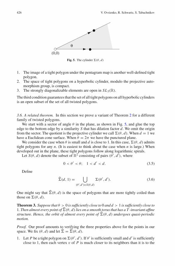
We start with a sector of angle θ in the plane, as shown in Fig. 5, and glue the topedge to the bottom edge by a similarity S that has dilation factor d. We omit the originfrom the sector. The quotient is the projective cylinder we call (θ, d). When d = 1 wehave a Euclidean cone surface. When θ = 2π we have the punctured plane.
We consider the case when θ is small and d is close to 1. In this case, (θ, d) admitstight polygons for any n. (It is easiest to think about the case when n is large.) Whendeveloped out in the plane, these tight polygons follow along logarithmic spirals.
Let S(θ, d) denote the subset of R2 consisting of pairs (θ ′, d ′), where
0 < θ ′ < θ; 1 < d ′ < d. (3.5)
Define
(d, 1) =⋃
(θ ′,d ′)∈S(θ,d)
(θ ′, d ′). (3.6)
One might say that (θ, d) is the space of polygons that are more tightly coiled thanthose on (θ, d).
Theorem 3. Suppose that θ > 0 is sufficiently close to 0 and d > 1 is sufficiently close to1. Then almost every point of (θ, d) lies on a smooth torus that has a T -invariant affinestructure. Hence, the orbit of almost every point of (θ, d) undergoes quasi-periodicmotion.
Proof. Our proof amounts to verifying the three properties above for the points in ourspace. We fix (θ, d) and let = (θ, d).
1. Let P be a tight polygon on (θ ′, d ′). If θ ′ is sufficiently small and d ′ is sufficientlyclose to 1, then each vertex v of P is much closer to its neighbors than it is to the
Pentagram Map: A Discrete Integrable System 427
origin. For this reason, the pentagram map acts on, and preserves, the set of tightpolygons on (θ ′, d ′). The same goes for the inverse of the pentagram map. Hence is a T -invariant subset of Pn .
2. Let Z(θ ′, d ′, α) denote the space of tight polygons on (θ ′, d ′) having Hilbertperimeter α. We consider these tight polygons equivalent if there is a similarityof (θ ′, d ′) that carries one to the other. A proof very much like the compactnessargument given in [19], for closed polygons, shows that Z(θ ′, d ′, α) is compact forθ ′ near 0 and d ′ near 1 and α arbitrary. Hence, the level sets of the Casimir functionsintersect in compact sets.
3. The similarity S is the monodromy for our tight polygons. S lifts to an element ofSL3(R) that has one real eigenvalue and two complex conjugate eigenvalues. Smallperturbations of S have the same property. Hence, is open in Pn .
We have assembled all the ingredients necessary for the proof of Theorem 2. The sameargument as above now establishes the result. Remark 3.10. The first property crucially uses the fact that θ is small. Consider the caseθ = 2π . It can certainly happen that P contains the origin in its hull but T (P) does not.We do not know the exact bounds on θ and d necessary for this construction.
4. Another Coordinate System in Space Pn
4.1. Polygons and difference equations. Consider two arbitrary n-periodic sequences(ai ), (bi ) with ai , bi ∈ R and i ∈ Z, such that ai+n = ai , bi+n = bi . Assume thatn �= 3 m. This will be our standing assumption whenever we work with the (a, b)-coordinates; its meaning will become clear shortly. We shall associate to these sequencesa difference equation of the form
Vi+3 = ai Vi+2 + bi Vi+1 + Vi , (4.1)
for all i .A solution V = (Vi ) is a sequence of numbers Vi ∈ R satisfying (4.1). Recall a
well-known fact that the space of solutions of (4.1) is 3-dimensional (any solution isdetermined by the initial conditions (V0, V1, V2)). We will often understand Vi as vectorsin R
3. The n-periodicity then implies that there exists a matrix M ∈ SL(3, R) called themonodromy matrix, such that Vi+n = M Vi .
Proposition 4.1. If n is not divisible by 3 then the space Pn is isomorphic to the spaceof the equations (4.1).
Proof. First note that since PGL(3, R) ∼= SL(3, R), every M ∈ PGL(3, R) correspondsto a unique element of SL(3, R) that (abusing the notations) we also denote by M .
A. Let (vi ), i ∈ Z be a sequence of points vi ∈ RP2 in general position with monodr-
omy M . Consider first an arbitrary lift of the points vi to vectors Vi ∈ R3 with the condi-
tion Vi+n = M(Vi ). The general position property implies that det(Vi , Vi+1, Vi+2) �= 0for all i . The vector Vi+3 is then a linear combination of the linearly independent vectorsVi+2, Vi+1, Vi , that is,
Vi+3 = ai Vi+2 + bi Vi+1 + ci Vi ,
for some n-periodic sequences (ai ), (bi ), (ci ). We wish to rescale: Vi = ti Vi , so that
det(Vi , Vi+1, Vi+2) = 1 (4.2)
428 V. Ovsienko, R. Schwartz, S. Tabachnikov
for all i . Condition (4.2) is equivalent to ci ≡ 1. One obtains the following system ofequations in (t1, . . . , tn):
ti ti+1ti+2 = 1/ det(Vi , Vi+1, Vi+2), i = 1, . . . , n − 2,
tn−1tnt1 = 1/ det(Vn−1, Vn, V1),
tnt1t2 = 1/ det(Vn, V1, V2).
This system has a unique solution if n is not divisible by 3. This means that any generictwisted n-gon in RP
2 has a unique lift to R3 satisfying (4.2). We proved that a twisted
n-gon defines Eq. (4.1) with n-periodic ai , bi .Furthermore, if (vi ) and (v′
i ), i ∈ Z are two projectively equivalent twisted n-gons,then they correspond to the same Eq. (4.1). Indeed, there exists A ∈ SL(3, R) such thatA(vi ) = v′
i for all i . One has, for the (unique) lift: V ′i = A(Vi ). The sequence (V ′
i ) thenobviously satisfies the same Eq. (4.1) as (Vi ).
B. Conversely, let (Vi ) be a sequence of vectors Vi ∈ R3 satisfying (4.1). Then every
three consecutive points satisfy (4.2) and, in particular, are linearly independent. There-fore, the projection (vi ) to RP
2 satisfies the general position condition. Moreover, sincethe sequences (ai ), (bi ) are n-periodic, (vi ) satisfies vi+n = M(vi ). It follows that everyEq. (4.1) defines a generic twisted n-gon. A choice of initial conditions (V0, V1, V2)
fixes a twisted polygon, a different choice yields a projectively equivalent one. Proposition 4.1 readily implies the next result.
Corollary 4.2. If n is not divisible by 3 then Pn = R2n.
We call the lift (Vi ) of the sequence (vi ) satisfying Eq. (4.1) with n-periodic (ai , bi )
canonical.
Remark 4.3. The isomorphism between the space Pn and the space of difference equa-tions (4.1) (for n �= 3m) goes back to the classical ideas of projective differentialgeometry. This is a discrete version of the well-known isomorphism between the spaceof smooth non-degenerate curves in RP
2 and the space of linear differential equations,see [17] and references therein and Sect. 6.1. The “arithmetic restriction” n �= 3m isquite remarkable.
Equations (4.1) and their analogs were already used in [9] in the context of integrablesystems; in the RP
1-case these equations were recently considered in [14] to study thediscrete versions of the Korteweg - de Vries equation. It is notable that an analogousarithmetic assumption n �= 2m is made in this paper as well.
Remark 4.4. Let us now comment on what happens if n is divisible by 3. A certainmodification of Proposition 4.1 holds in this case as well. Given a twisted n-gon (vi )
with monodromy M , lift points v0 and v1 arbitrarily as vectors V0, V1 ∈ R3, and then
continue lifting consecutive points so that the determinant condition (4.2) holds. Thisimplies that Eq. (4.1) holds as well.
One has:
M(Vi ) = ti Vi+n (4.3)
for non-zero reals ti , and (4.2) implies that ti ti+1ti+2 = 1 for all i ∈ Z. It follows thatthe sequence ti is 3-periodic; let us write t1+3 j = α, t2+3 j = β, t3 j = 1/(αβ). Applyingthe monodromy linear map M to (4.1) and using (4.3), we conclude that
an+i = ti+2
tiai , bn+i = ti+1
tibi ,
Pentagram Map: A Discrete Integrable System 429
that is,
an+3 j = αβ2 a3 j , an+3 j+1 = 1
α2βa3 j+1, an+3 j+2 = α
βa3 j+2,
bn+3 j = α2βb3 j , bn+3 j+1 = β
αb3 j+1, bn+3 j+2 = 1
αβ2 b3 j+2.
(4.4)
We are still free to rescale V0 and V1. This defines an action of the group R∗ × R
∗:
V0 �→ uV0, V1 �→ vV1, u �= 0, v �= 0.
The action of the group R∗ × R
∗ on the coefficients (ai , bi ) is as follows:
a3 j �→ u2v a3 j , a3 j+1 �→ v
ua3 j+1, a3 j+2 �→ 1
uv2 a3 j+2,
b3 j �→ u
vb3 j , b3 j+1 �→ uv2 b3 j+1, b3 j+2 �→ 1
u2vb3 j+2.
(4.5)
When n �= 3m, according to (4.4), this action makes it possible to normalize all ti to 1which makes the lift canonical. However, if n = 3m then the R
∗ × R∗-action on ti is
trivial, and the pair (α, β) ∈ R∗ × R
∗ is a projective invariant of the twisted polygon.One concludes that Pn is the orbit space
[{(a0, . . . , an−1, b0, . . . , bn−1)}/(R∗ × R∗)] × (R∗ × R
∗)
with respect to R∗ ×R
∗-action (4.5). This statement replaces Proposition 4.1 in the caseof n = 3m.
It would be interesting to understand the geometric meaning of the “obstruction”(α, β). If the obstruction is trivial, that is, if α = β = 1, then there exists a 2-parameterfamily of canonical lifts, but if the obstruction is non-trivial then no canonical lift exists.
4.2. Relation between the two coordinate systems. We now have two coordinate sys-tems, (xi , yi ) and (ai , bi ). Assuming that n is not divisible by 3, let us calculate therelations between the two systems.
Lemma 4.5. One has:
xi = ai−2
bi−2 bi−1, yi = − bi−1
ai−2 ai−1. (4.6)
Proof. Given four vectors a, b, c, d in R3, the intersection line of the planes Span(a, b)
and Span(c, d) is spanned by the vector (a ×b)× (c ×d). Note that the volume elementequips R
3 with the bilinear vector product:
R3 × R
3 →(R
3)�
.
Using the identity
(a × b) × (b × c) = det(a, b, c) b, (4.7)
and the recurrence (4.1), let us compute lifts of the quadruple of points
(vi−1, vi , (vi−1, vi ) ∩ (vi+1, vi+2), (vi−1, vi ) ∩ (vi+2, vi+3))
430 V. Ovsienko, R. Schwartz, S. Tabachnikov
involved in the left corner cross-ratio. One has
Vi−1 = Vi+2 − ai−1 Vi+1 − bi−1 Vi .
Furthermore, it is easy to obtain the lift of the intersection points involved in the leftcorner cross-ratio. For instance, (vi−1, vi ) ∩ (vi+1, vi+2) is
(Vi−1 × Vi ) × (Vi+1 × Vi+2) = ((Vi+2 − ai−1 Vi+1 − bi−1 Vi ) × Vi ) × (Vi+1 × Vi+2)
= Vi+2 − ai−1 Vi+1.
One finally obtains the following four vectors in R3:
(Vi+2−ai−1 Vi+1−bi−1, Vi , Vi , Vi+2−ai−1 Vi+1, bi Vi+2−ai−1 Vi −ai−1 bi Vi+1).
Similarly, for the points involved in the right corner cross-ratio
(ai Vi+2 + bi , Vi+1 + Vi , Vi+2, bi Vi+1 + Vi , bi Vi+2 − ai−1 Vi − ai−1 bi Vi+1) .
Next, given four coplanar vectors a, b, c, d in R3 such that
c = λ1 a + λ2 b, d = μ1 a + μ2 b,
where λ1, λ2, μ1, μ2 are arbitrary constants, the cross-ratio of the lines spanned by thesevectors is given by
[a, b, c, d] = λ2μ1 − λ1μ2
λ2μ1.
Applying this formula to the two corner cross-ratios yields the result. Formula (4.6) implies the following relations:
xi yi = − 1
ai−1 bi−2, xi+1 yi = − 1
ai−2 bi,
ai
ai−3= xi yi−1
xi+1 yi+1,
bi
bi−3= xi−1 yi−1
xi+1 yi,
(4.8)
that will be of use later.
Remark 4.6. If n is a multiple of 3 then the coefficients ai and bi are not well definedand they are not n-periodic anymore; however, according to formulas (4.4) and (4.5),the right hand sides of formulas (4.6) are still well defined and are n-periodic.
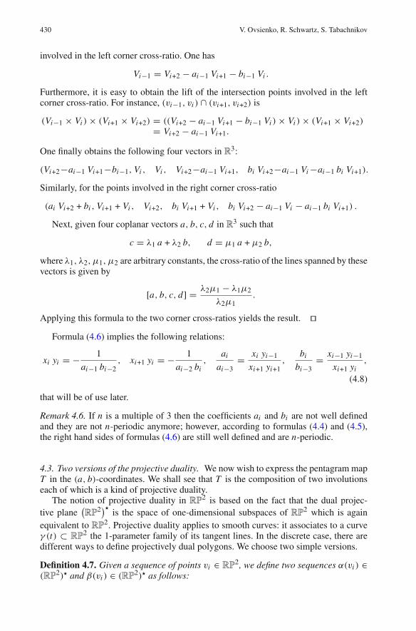
4.3. Two versions of the projective duality. We now wish to express the pentagram mapT in the (a, b)-coordinates. We shall see that T is the composition of two involutionseach of which is a kind of projective duality.
The notion of projective duality in RP2 is based on the fact that the dual projec-
tive plane(RP
2)�is the space of one-dimensional subspaces of RP
2 which is againequivalent to RP
2. Projective duality applies to smooth curves: it associates to a curveγ (t) ⊂ RP
2 the 1-parameter family of its tangent lines. In the discrete case, there aredifferent ways to define projectively dual polygons. We choose two simple versions.
Definition 4.7. Given a sequence of points vi ∈ RP2, we define two sequences α(vi ) ∈
(RP2)� and β(vi ) ∈ (RP
2)� as follows:

Pentagram Map: A Discrete Integrable System 431
Fig. 6. Projective dual for smooth curves and polygons
Fig. 7. Iteration of the duality maps: α2(vi )=α(vi ) ∩ α(vi+1), β2(vi )=β(vi−1) ∩ β(vi+1) and (α ◦ β)
(vi ) = β(vi ) ∩ β(vi+1)
1. α(vi ) is the line (vi , vi+1),2. β(vi ) is the line (vi−1, vi+1),
see Fig. 6.
Clearly, α and β commute with the natural PGL(3, R)-action and therefore are well-defined on the space Pn . The composition of α and β is precisely the pentagram map T .
Lemma 4.8. One has
α2 = τ, β2 = Id, α ◦ β = T, (4.9)
where τ is the cyclic permutation:
τ(vi ) = vi+1. (4.10)
Proof. The composition of the maps α and β, with themselves and with each other,associates to the corresponding lines (viewed as points of (RP
2)�) their intersections,see Fig. 7.
The map (4.10) defines the natural action of the group Z on Pn . All the geometricand algebraic structures we consider are invariant with respect to this action.
4.4. Explicit formula for α. It is easy to calculate the explicit formula of the map α interms of the coordinates (ai , b j ). As usual, we assume n �= 3 m.
Lemma 4.9. Given a twisted n-gon with monodromy (vi ), i ∈ Z represented by a dif-ference equation (4.1), the n-gon (α(vi )), i ∈ Z is represented by the Eq. (4.1) withcoefficients
α∗(ai ) = −bi+1, α∗(bi ) = −ai , (4.11)
where, as usual, a∗ stands for the pull-back of the coordinate functions.

432 V. Ovsienko, R. Schwartz, S. Tabachnikov
Proof. Consider the canonical lift (Vi ) to R3. Let Ui = Vi × Vi+1 ∈ (R3)�. This is obvi-
ously a lift of the sequence (α(vi )) to (R3)�. We claim that (Ui ) is, in fact, a canonicallift.
Indeed, Ui is a lift of ui since Vi × Vi+1 is orthogonal to Vi and to Vi+1. Next, usingthe identity (4.7) one has
det(Ui ×Ui+1, Ui+1×Ui+2, Ui+2×Ui+3) = [(Ui ×Ui+1)×(Ui+1×Ui+2)] · (Ui+2×Ui+3)
= Ui+1 · (Ui+2 × Ui+3) = det(Ui+1, Ui+2, Ui+3) = 1.
It follows that the sequence Ui ∈ R3 satisfies the equation
Ui+3 = α∗(ai ) Ui+2 + α∗(bi ) Ui+1 + Ui
with some α∗(ai ) and α∗(bi ). Let us show that these coefficients are, indeed, given by(4.11). For all i , one has
Ui+1 · Vi = 1, Ui · Vi+2 = 1, Ui+3 · Vi+3 = 0.
Using (4.1), the last identity leads to:
α∗(bi ) Ui+1 · Vi + ai Ui · Vi+2 = 0.
Hence α∗(bi ) = −ai . The first identity in (4.11) follows from formula (4.9). Indeed,one has α∗(α∗(ai )) = ai+1 and α∗(α∗(bi )) = bi+1, and we are done.
4.5. Recurrent formula for β. The explicit formula for the map β is more complicated,and we shall give a recurrent expression.
Lemma 4.10. Given an n-gon (vi ), i ∈ Z represented by a difference equation (4.1),the n-gon (β(vi )), i ∈ Z is represented by the Eq. (4.1) with coefficients
β∗(ai ) = −λi bi−1
λi+2, β∗(bi ) = −λi+3 ai+1
λi+1, (4.12)
where the coefficients λi are uniquelly defined by
λiλi+1λi+2 = − 1
1 + bi−1ai(4.13)
for all i .
Proof. The lift of the map β to R3 takes Vi to Wi = λi Vi−1 × Vi+1, where the coeffi-
cients λi are chosen in such a way that det(Wi , Wi+1, Wi+2) = 1 for all i . The sequenceWi ∈ R
3 satisfies the equation
Wi+3 = β∗(ai ) Wi+2 + β∗(bi ) Wi+1 + Wi .
To find β∗(ai ) and β∗(bi ), one substitutes Wi = λi Vi−1 × Vi+1, and then, using (4.1),expresses each V as a linear combination of Vi , Vi+1, Vi+2. The above equation is thenequivalent to the following one:
(β∗(ai ) λi+2 + bi−1 λi
)Vi × Vi+1
+(ai+1 λi+3 + β∗(bi ) λi+1
)Vi × Vi+2
+((1 + bi ai+1) λi+3 + β∗(ai ) ai λi+2 − λi
)Vi+1 × Vi+2 = 0.

Pentagram Map: A Discrete Integrable System 433
Since the three terms are linearly independent, one obtains three relations. The first twoequations lead to (4.12) while the last one gives the recurrence
λi+3 = λi1 + ai bi−1
1 + ai+1 bi.
On the other hand, one has
λi λi+1 λi+2 det (Vi−1 × Vi+1, Vi × Vi+2, Vi+1 × Vi+3) = 1.
Once again, expressing each V as a linear combination of Vi , Vi+1, Vi+2, yields
λiλi+1λi+2 (1 + ai bi−1) = −1,
and one obtains (4.13).
4.6. Formulas for the pentagram map. We can now describe the pentagram map in termsof (a, b)-coordinates and to deduce formulas (2.4).
Proposition 4.11. (i) One has:
T ∗(xi ) = xi1 − xi−1 yi−1
1 − xi+1 yi+1, T ∗(yi ) = yi+1
1 − xi+2 yi+2
1 − xi yi.
(ii) Assume that n = 3m + 1 or n = 3m + 2; in both cases,
T ∗(ai ) = ai+2
m∏
k=1
1 + ai+3k+2 bi+3k+1
1 + ai−3k+2 bi−3k+1, T ∗(bi ) = bi−1
m∏
k=1
1 + ai−3k−2 bi−3k−1
1 + ai+3k−2 bi+3k−1.
(4.14)
Proof. According to Lemma 4.8, T = α ◦ β. Combining Lemmas 4.9 and 4.10, oneobtains the expression:
T ∗(ai ) = λi+4 ai+2
λi+2, T ∗(bi ) = λi bi−1
λi+2,
where λi are as in (4.13). Equation (4.6) then gives
T ∗(xi ) = T ∗(ai−2)
T ∗(bi−2) T ∗(bi−1)= λi+2 ai
λi
λi
λi−2 bi−3
λi+1
λi−1 bi−2
= ai
bi−2 bi−3
1 + bi−3 ai−2
1 + bi−1 ai= ai−3
bi−2 bi−3
1 + bi−3 ai−2
1 + bi−1 ai
ai
ai−3
= xi−1
1 − 1xi−1 yi−1
1 − 1xi+1 yi+1
xi yi−1
xi+1 yi+1= xi
1 − xi−1 yi−1
1 − xi+1 yi+1,
and similarly for yi . We thus proved formula (2.4). To prove (4.14), one now uses (4.8).

434 V. Ovsienko, R. Schwartz, S. Tabachnikov
+
Fig. 8. The Poisson bracket for n=5 and n = 7
4.7. The Poisson bracket in the (a, b)-coordinates. The explicit formula of the Poissonbracket in the (a, b)-coordinates is more complicated than (2.16). Recall that n is not amultiple of 3 so that we assume n = 3m + 1 or n = 3m + 2. In both cases the Poissonbracket is given by the same formula.
Proposition 4.12. The Poisson bracket (2.16) can be rewritten as follows:
{ai , a j } =m∑
k=1
(δi, j+3k − δi, j−3k
)ai a j ,
{ai , b j } = 0,
{bi , b j } =m∑
k=1
(δi, j−3k − δi, j+3k
)bi b j .
(4.15)
Proof. One checks using (4.5) that the brackets between the coordinate functions (xi , y j )
coincide with (2.16).
Example 4.13. a) For n = 4, the bracket is
{ai , a j } = (δi, j+1 − δi, j−1
)ai a j
(and with opposite sign for b), the other terms vanish.b) For n = 5, the non-zero terms are:
{ai , a j } = (δi, j+2 − δi, j−2
)ai a j ,
corresponding to the “pentagram” in Fig. 8.c) For n = 7, one has:
{ai , a j } = (δi, j+1 − δi, j−1 − δi, j+3 + δi, j−3
)ai a j .
d) For n = 8, the result is
{ai , a j } = (δi, j+2 − δi, j−2 − δi, j+3 + δi, j−3
)ai a j .
5. Monodromy Invariants in (a, b)-Coordinates
The (a, b)-coordinates are especially well adapted to the computation of the monodr-omy matrix and the monodromy invariants. Such a computation provides an alternativededuction of the invariants (2.11), independent of [21].

Pentagram Map: A Discrete Integrable System 435
5.1. Monodromy matrices. Consider the 3 × ∞ matrix M constructed recurrently asfollows: the columns C0, C1, C2, . . . satisfy the relation
Ci+3 = ai Ci+2 + bi Ci+1 + Ci , (5.1)
and the initial 3 × 3 matrix (C0, C1, C2) is unit. The matrix M contains the monodromymatrices of twisted n-gons for all n; namely, the following result holds.
Lemma 5.1. The 3×3 minor Mn = (Cn, Cn+1, Cn+2) represents the monodromy matrixof twisted n-gons considered as a polynomial function in a0, . . . , an−1, b0, . . . , bn−1.
Proof. The recurrence (5.1) coincides with (4.1), see Sect. 4.1. It follows that Mnrepresents the monodromy of twisted n-gons in the basis C0, C1, C2.
Let
N j =⎛
⎝0 0 11 0 b j0 1 a j
⎞
⎠ .
The recurrence (5.1) implies the following statement.
Lemma 5.2. One has: Mn = N0 N1 . . . Nn−1. In particular, det Mn = 1.
To illustrate, the beginning of the matrix M is as follows:⎛
⎝1 0 0 1 a1 a1a2 + b2 . . .
0 1 0 b0 b0a1 + 1 b0a1a2 + a2 + b0b2 . . .
0 0 1 a0 a0a1 + b1 a0a1a2 + b1a2 + a0b1 + 1 . . .
⎞
⎠ .
The dihedral symmetry σ , that reverses the orientation of a polygon, replaces themonodromy matrices by their inverses and acts as follows:
σ : ai �→ −b−i , bi �→ −a−i ;this follows from rewriting Eq. (4.1) as
Vi = −bi Vi+1 − ai Vi+2 + Vi+3,
or from Lemma 4.5.1
Consider the rescaling 1-parameter group
ϕτ : ai �→ eτ ai , bi �→ e−τ bi .
It follows from Lemma 4.5 that the action on the corner invariants is as follows:
xi �→ e3τ xi , yi �→ e−3τ yi .
Thus our rescaling is essentially the same as the one in (2.5) with t = e3τ .The trace of Mn is a polynomial Fn(a0, . . . , an−1, b0, . . . , bn−1). Denote its homo-
geneous components in s := eτ by I j , j = 0, . . . , [n/2]; these are the monodromyinvariants. One has Fn = ∑
I j . The s-weight of I j is given by the formula:
w( j) = 3 j − k if n = 2k, and w( j) = 3 j − k + 1 if n = 2k + 1 (5.2)
1 Since all the sums we are dealing with are cyclic, we slightly abuse the notation and ignore a cyclic shiftin the definition of σ in the (a, b)-coordinates.
436 V. Ovsienko, R. Schwartz, S. Tabachnikov
(this will follow from Proposition 5.3 in the next section). For example, M4 is the matrix⎛
⎝a1 a1a2+b2 a1a2a3+a3b2+a1b3+1
a1b0 +1 a1a2b0 +a2 +b0b2 a1a2a3b0 +a2a3+a3b0b2 +a1b0b3+b3+b0a0a1+b1 a0a1a2+a2b1+a0b2+1 a0a1a2a3+a2a3b1+a0a3b2+a0a1b3+a0 +a3+b1b3
⎞
⎠
and
I0 =b0b2 +b1b3, I1 =a0 +a1+a2+a3+b0a1a2 +b1a2a3+b2a3a0 +b3a0a1, I2 =a0a1a2a3.
Likewise, for n = 5,
I0 =∑
(b0 + b0b2a3), I1 =∑
(a0a1 + b0a1a2a3), I2 = a0a1a2a3a4,
where the sums are cyclic over the indices 0, . . . , 4.One also has the second set of monodromy invariants J0, . . . , Jk constructed from
the inverse monodromy matrix, that is, applying the dihedral involution σ to I0, . . . , Ik .
5.2. Combinatorics of the monodromy invariants. We now describe the polynomialsIi , Ji and their relation to the monodromy invariants Ek, Ok .
Label the vertices of an oriented regular n-gon by 0, 1, . . . , n − 1. Consider markingof the vertices by the symbols a, b and ∗ subject to the rule: each marking should becoded by a cyclic word W in symbols 1, 2, 3, where 1 = a, 2 = ∗ b, 3 = ∗∗∗. Call suchmarkings admissible. If p, q, r are the occurrences of 1, 2, 3 in W then p + 2q + 3r = n;define the weight of W as p − q. Given a marking as above, take the product of therespective variables ai or bi that occur at vertex i ; if a vertex is marked by ∗ then itcontributes 1 to the product. Denote by Tj the sum of these products over all markingsof weight j . Then A := Tk is the product of all ai ; let B be the product of all bi ; herek = [n/2].Proposition 5.3. The monodromy invariants I j coincide with the polynomials Tj . Onehas:
E j = Ik− j
Afor j = 1, . . . , k, and En = (−1)n B
A2 .
J j are described similarly by the rule 1 = b, 2 = a ∗, 3 = ∗ ∗ ∗, and are similarlyrelated to O j :
O j = (−1)n+ j Jk− j
Bfor j = 1, . . . , k, and On = A
B2 .
Proof. First, we claim that the trace Fn is invariant under cyclic permutations of theindices 0, 1, . . . , n − 1.
Indeed, impose the n-periodicity condition: ai+n = ai , bi+n = bi . Let Vi be as (4.1).The matrix Mn takes (V0, V1, V2) to (Vn, Vn+1, Vn+2). Then the matrix (V1, V2, V3) →(Vn+1, Vn+2, Vn+3) is conjugated to Mn and hence has the same trace. This trace isFn(a1, b1, . . . , an, bn), and due to n-periodicity, this equals Fn(a1, b1, . . . , a0, b0). ThusFn is cyclically invariant.
Now we argue inductively on n. Assume that we know that I j = Tj for j = n −2, n − 1, n. Consider Fn+1. Given an admissible labeling of n − 2, n − 1 or n-gon, onemay insert ∗∗∗, ∗ b or a between any two consecutive vertices, respectively, and obtain

Pentagram Map: A Discrete Integrable System 437
an admissible labeling of n + 1-gon. All admissible labeling are thus obtained, possibly,in many different ways.
We claim that Fn+1 contains the cyclic sums corresponding to all admissible labeling.Indeed, consider an admissible cyclic sum in Fn−2 corresponding to a labeled n −2-gonL . This is a cyclic sum of monomials in a0, . . . , bn−3; these monomials are located inthe matrix M on the diagonal of its minor Mn−2. By recurrence (5.1), the same mono-mials will appear on the diagonal of Mn+1, but now they must contribute to a cyclic sumof variables a0, . . . , bn . These sums correspond to the labelings of n + 1-gon that areobtained from L by inserting ∗ ∗ ∗ between two consecutive vertices.
Likewise, consider a term in Fn−1, a cyclic sum of monomials in a0, . . . , bn−2corresponding to a labeled n − 1-gon L . By (5.1), these monomials are to be multi-plied by bn−2, bn−1 or bn (depending on whether they appear in the first, second orthird row of M) and moved 2 units right in the matrix M , after which they contribute tothe cyclic sums in Fn+1. As before, the respective sums correspond to the labelings ofn + 1-gon obtained from L by inserting ∗ b between two consecutive vertices. Similarlyone deals with a contribution to Fn+1 from Fn : this time, one inserts symbol a.
Our next claim is that each admissible term appears in Fn+1 exactly once. Supposenot. Using cyclicity, assume this is a monomial an P (or, similarly, bn P). Where coulda monomial an P come from? Only from the bottom position of the column Cn+2 (onceagain, according to recurrence (5.1)). But then the monomial P appears at least twice inthis position, hence in Fn , which contradicts our induction assumption. This completesthe proof that I j = Tj .
Now let us prove that E j = Ik− j/A. Consider E j as a function of x, y and switch tothe (a, b)-coordinates using Lemma 4.5:
x1 = a−1
b−1b0, y1 = − b0
a−1a0
and its cyclic permutations. Then
y0x1 y1 = 1
a−2a−1a0
and the cyclic permutations. An admissible monomial in E j then contributes the factor−bi/(ai−1ai ) for each singleton yi+1 and 1/(ai−2ai−1ai ) for each triple yi xi+1 yi+1.
Admissibility implies that no index appears twice. Clear denominators by multiplyingby A, the product of all a’s. Then, for each singleton yi+1, we get the factor −bi and emptyspace ∗ at the previous position i − 1, because there was ai−1 in the denominator and,for each triple yi xi+1 yi+1, we get empty spaces ∗∗∗ at positions i −2, i −1, i . All other,“free”, positions are filled with a’s. In other words, the rule 1 = a, 2 = ∗ b, 3 = ∗ ∗ ∗applies. The signs are correct as well, and the result follows.
Finally, En is the product of all yi+1, that is, of the terms −bi/(ai−1ai ). This productequals (−1)n B/A2. Remark 5.4. Unlike the invariants Ok, Ek , there are no signs involved: all the terms inpolynomials Ii are positive.
Similarly to Remark 4.6, the next lemma shows that one can use Proposition 5.3 evenif n is a multiple of 3. In particular, this will be useful in Theorem 4 in the next section.
Lemma 5.5. If n is a multiple of 3 then the polynomials I j , J j of variables a0, . . . , bn−1are invariant under the action of the group R
∗ × R∗ given in (4.5).

438 V. Ovsienko, R. Schwartz, S. Tabachnikov
Proof. Recall that, by Lemma 5.2, Mn = N0 N1 . . . Nn−1, where
N j =⎛
⎝0 0 11 0 b j0 1 a j
⎞
⎠ .
The action of R∗ × R
∗ on the matrices N j depends on j mod 3 and is given by the nextformulas:
⎛
⎝0 0 11 0 b00 1 a0
⎞
⎠ �→⎛
⎝0 0 11 0 u
vb0
0 1 u2v a0
⎞
⎠ =⎛
⎝1 0 00 u
v0
0 0 u2v
⎞
⎠
⎛
⎝0 0 11 0 b00 1 a0
⎞
⎠
⎛
⎝vu 0 00 1
u2v0
0 0 1
⎞
⎠ ,
⎛
⎝0 0 11 0 b10 1 a1
⎞
⎠ �→⎛
⎝0 0 11 0 uv2 b10 1 v
u a1
⎞
⎠ =⎛
⎝1 0 00 uv2 00 0 v
u
⎞
⎠
⎛
⎝0 0 11 0 b10 1 a1
⎞
⎠
⎛
⎝1
uv2 0 00 u
v0
0 0 1
⎞
⎠ ,
⎛
⎝0 0 11 0 b20 1 a2
⎞
⎠ �→⎛
⎝0 0 11 0 1
u2vb2
0 1 1uv2 a2
⎞
⎠ =⎛
⎝1 0 00 1
u2v0
0 0 1uv2
⎞
⎠
⎛
⎝0 0 11 0 b20 1 a2
⎞
⎠
⎛
⎝u2v 0 0
0 uv2 00 0 1
⎞
⎠ .
Note that⎛
⎝vu 0 00 1
u2v0
0 0 1
⎞
⎠
⎛
⎝1 0 00 uv2 00 0 v
u
⎞
⎠ = v
uE,
⎛
⎝1
uv2 0 00 u
v0
0 0 1
⎞
⎠
⎛
⎝1 0 00 1
u2v0
0 0 1uv2
⎞
⎠ = 1
uv2 E,
and⎛
⎝u2v 0 0
0 uv2 00 0 1
⎞
⎠
⎛
⎝1 0 00 u
v0
0 0 u2v
⎞
⎠ = u2v E,
where E is the unit matrix. Therefore the R∗ × R
∗-action on Mn is as follows:
Mn �→ 1
u2v
⎛
⎝1 0 00 u
v0
0 0 u2v
⎞
⎠ N0 N1 . . . Nn−1
⎛
⎝u2v 0 0
0 uv2 00 0 1
⎞
⎠ ∼ Mn,
where ∼ means “is conjugated to”. It follows that the trace of Mn , as a polynomial ina0, . . . , bn−1, is R
∗ × R∗-invariant, and so are all its homogeneous components.
5.3. Closed polygons. A closed n-gon (as opposed to a merely twisted one) is charac-terized by the condition that Mn = I d. This implies that
∑I j = 3 (and, of course,∑
J j = 3 as well). There are other linear relations on the monodromy invariants whichwe discovered in computer experiments. All combined, we found five identities.
Theorem 4. For a closed n-gon, one has:
k∑
j=0
I j =k∑
j=0
J j = 3,
k∑
j=0
w( j)I j =k∑
j=0
w( j)J j = 0,
k∑
j=0
w( j)2(I j − J j ) = 0,
where k = [n/2] and w( j) are the weights (5.2).

Pentagram Map: A Discrete Integrable System 439
Proof. The monodromy M ∈ SL(3, R) is a matrix-valued polynomial function of ai , bi ,and M(τ ) = M ◦ ϕτ , where ϕτ is the scaling action
ai �→ eτ ai , bi �→ e−τ bi .
The characterization of Cn is M(0) = I d.Let eλ1 , eλ2 , eλ3 be the eigenvalues of M(τ ) considered as functions of ai , bi , τ . Then
λi = 0 for τ = 0 and each i = 1, 2, 3, and
λ1 + λ2 + λ3 = 0 (5.3)
identically. The eigenvalues of M−1 are similar with negative λs as exponents. Thedefinition of I (a, b) and J (a, b) implies:
eλ1 + eλ2 + eλ3 =∑
eτw( j) I j , e−λ1 + e−λ2 + e−λ3 =∑
e−τw( j) J j , (5.4)
where w( j) are the weights. Setting τ = 0 in (5.4) we obtain the obvious relations∑I j = ∑
J j = 3. Differentiating (5.4) with respect to τ and setting τ = 0, we get
3∑
i=1
λ′i (0) =
∑w( j)I j =
∑w( j)J j .
By (5.3), the left hand side is zero, and we obtain two other relations stated in the theorem.Differentiate (5.4) twice and set τ = 0:
3∑
i=1
λ′′i (0) + λ′
i (0)2 =∑
w( j)2 I j ,
3∑
i=1
−λ′′i (0) + λ′
i (0)2 =∑
w( j)2 J j .
Subtract and use the fact that∑3
i=1 λ′′i (0) = 0 (as follows from (5.3) by differentiating
in τ twice) to obtain:∑
w( j)2(I j − J j ) = 0. (5.5)
This is the fifth relation of the theorem. Example 5.6. In the cases n = 4 and n = 5, it is easy to solve the equation Mn = I d.For n = 4, the solution is a single point
a0 = a1 = a2 = a3 = 1, b0 = b1 = b2 = b3 = −1,
and then I0 = 2, I1 = 0, I2 = 1. For n = 5, one has a 2-parameter set of solutions withfree parameters x, y:
a0 = x, a1 = y, a2 = − 1 + x
1 − xy, a3 = −(1 − xy), a4 = − 1 + y
1 − xy,
and bi = −ai+2. Hence
I0 = J0 = 2 − z, I1 = J1 = 1 + 2z, I2 = J2 = −z with z = xy(1 + x)(1 + y)
1 − xy.
Remark 5.7. Cn has codimension 8 in Pn , and we have the five relations of Theorem 4.We conjecture that there are no other relations between the monodromy invariants thathold identically on Cn .

440 V. Ovsienko, R. Schwartz, S. Tabachnikov
6. Continuous Limit: The Boussinesq Equation
Since the theory of infinite-dimensional integrable systems on functional spaces is muchmore developed than the theory of discrete integrable systems, it is important to inves-tigate the n → ∞ “continuous limit” of the pentagram map.
It turns out that the continuous limit of T is the classical Boussinesq equation. This isquite remarkable since the Boussinesq equation and its discrete analogs are thoroughlystudied but, to the best of our knowledge, their geometrical interpretation remainedunknown.
We will also show that the Poisson bracket (2.16) can be viewed as a discrete versionof the well-known first Poisson structure of the Boussinesq equation.
6.1. Non-degenerate curves and differential operators. We understand the continuouslimit of a twisted n-gon as a smooth parametrized curve γ : R → RP
2 with monodromy:
γ (x + 1) = M(γ (x)), (6.1)
for all x ∈ R, where M ∈ P SL(3, R) is fixed. The assumption that every three consec-utive points are in general position corresponds to the assumption that the vectors γ ′(x)
and γ ′′(x) are linearly independent for all x ∈ R. A curve γ satisfying these conditionsis usually called non-degenerate.
As in the discrete case, we consider classes of projectively equivalent curves. Thecontinuous analog of the space Pn , is then the space, C, of parametrized non-degener-ate curves in RP
2 up to projective transformations. The space C is very well known inclassical projective differential geometry, see, e.g., [17] and references therein.
Proposition 6.1. There exists a one-to-one correspondence between C and the space oflinear differential operators on R:
A =(
d
dx
)3
+ u(x)d
dx+ v(x), (6.2)
where u and v are smooth periodic functions.
This statement is classical, but we give here a sketch of the proof.
Proof. A non-degenerate curve γ (x) in RP2 has a unique lift to R
3, that we denote by�(x), satisfying the condition that the determinant of the vectors �(x), �′(x), �′′(x)
(the Wronskian) equals 1 for every x :∣∣�(x) �′(x) �′′(x)
∣∣ = 1. (6.3)
The vector �′′′(x) is a linear combination of �(x), �′(x), �′′(x) and the condition (6.3) isequivalent to the fact that this combination does not depend on �′′(x). One then obtains:
�′′′(x) + u(x) �′(x) + v(x) �(x) = 0.
Two curves in RP2 correspond to the same operator if and only if they are projectively
equivalent.Conversely, every differential operator (6.2) defines a curve in RP
2. Indeed, the spaceof solutions of the differential equation A f = 0 is 3-dimensional. At any point x ∈ R,one considers the 2-dimensional subspace of solutions vanishing at x . This defines acurve in the projectivization of the space dual to the space of solutions.
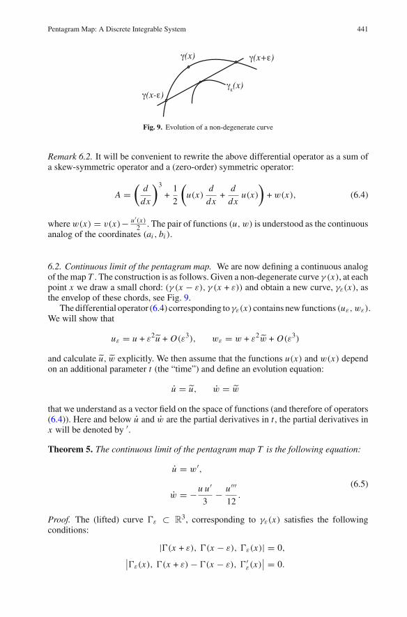
Pentagram Map: A Discrete Integrable System 441
Fig. 9. Evolution of a non-degenerate curve
Remark 6.2. It will be convenient to rewrite the above differential operator as a sum ofa skew-symmetric operator and a (zero-order) symmetric operator:
A =(
d
dx
)3
+1
2
(u(x)
d
dx+
d
dxu(x)
)+ w(x), (6.4)
where w(x) = v(x)− u′(x)2 . The pair of functions (u, w) is understood as the continuous
analog of the coordinates (ai , bi ).
6.2. Continuous limit of the pentagram map. We are now defining a continuous analogof the map T . The construction is as follows. Given a non-degenerate curve γ (x), at eachpoint x we draw a small chord: (γ (x − ε), γ (x + ε)) and obtain a new curve, γε(x), asthe envelop of these chords, see Fig. 9.
The differential operator (6.4) corresponding toγε(x) contains new functions (uε, wε).We will show that
uε = u + ε2u + O(ε3), wε = w + ε2w + O(ε3)
and calculate u, w explicitly. We then assume that the functions u(x) and w(x) dependon an additional parameter t (the “time”) and define an evolution equation:
u = u, w = w
that we understand as a vector field on the space of functions (and therefore of operators(6.4)). Here and below u and w are the partial derivatives in t , the partial derivatives inx will be denoted by ′.
Theorem 5. The continuous limit of the pentagram map T is the following equation:
u = w′,
w = −u u′
3− u′′′
12.
(6.5)
Proof. The (lifted) curve �ε ⊂ R3, corresponding to γε(x) satisfies the following
conditions:
|�(x + ε), �(x − ε), �ε(x)| = 0,∣∣�ε(x), �(x + ε) − �(x − ε), �′
ε(x)∣∣ = 0.

442 V. Ovsienko, R. Schwartz, S. Tabachnikov
We assume that the curve �ε(x) is of the form:
�ε = γ + ε A + ε2 B + (ε3),
where A and B are some vector-valued functions. The above conditions easily implythat A is proportional to �, while B satisfies:
∣∣�(x), �′(x), B ′(x)∣∣ = 0,
12
∣∣�(x), �′(x), �′′(x)∣∣ +
∣∣�(x), �′(x), B(x)∣∣ = 0.
It follows that B = 12�′′ + g�, where g is a function. We proved that the curve �ε(x) is
of the form:
�ε = (1 + ε f + ε2g
)� + ε2
2 �′′ + (ε3),
where f and g are some functions.It remains to find f and g and the corresponding differential operator. To this end
one has to use the normalization condition (6.3).
Lemma 6.3. The condition (6.3) implies f (x) ≡ 0 and g(x) = u(x)3 .
Proof. A straightforward computation. One has finally the following expression for the lifted curve:
�ε =(
1 +ε2
3u
)� +
ε2
2�′′ + (ε3). (6.6)
We are ready to find the new functions uε, vε such that
�′′′ε (x) + uε(x) �′
ε(x) + vε(x) �ε(x) = 0.
After a straightforward calculation, using the additional formula
�(V ) = −(2u′ + v) �′′ − (u′′ + 2v′ − u2) �′ − (v′′ − uv) �,
one gets directly from (6.6):
uε = u + ε2(
v′ − u′′
2
), vε = v + ε2
(v′′
2− uu′
3− u′′′
3
).
The result follows. Remark 6.4. Equation (6.5) is equivalent to the following differential equation:
u = −(u2
)′′
6− u(I V )
12,
which is nothing else but the classical Boussinesq equation.
Remark 6.5. It is not hard to compute that the continuous limit of the scaling symmetryis given by the formula:
u(x) �→ u(x), w(x) �→ w(x) + t,
where t is a constant.

Pentagram Map: A Discrete Integrable System 443
Remark 6.6. The fact that the continuous limit of the pentagram map is the Boussinesqequation is discovered in [19] (not much details are provided). The computation in [19]is made in an affine chart R
2 ⊂ RP2. In this lift, different from the canonical one
(characterized by constant Wronskian), one obtains the curve flow
� = −1
3
[�′, �′′′][�′, �′′] �′ +
1
2�′′,
where [., .] is the cross-product; this is equivalent to Eq. (6.6) (we omit a rather tediousverification of this equivalence).
6.3. The constant Poisson structure. Eq. (6.5) is integrable. In particular, it isHamiltonian with respect to (two) Poisson structures on the space of functions (u, w).We describe here the simplest Poisson structure usually called the first Poisson structureof the Boussinesq equation.
Consider the space of functionals of the form
H(u, w) =∫
S1h(u, u′, . . . , w,w′, . . .) dx,
where h is a polynomial. The variational derivatives, δu H and δw H , are the smoothfunctions on S1 given by the Euler-Lagrange formula, e.g.,
δu H = ∂h
∂u−
(∂h
∂u′
)′+
(∂h
∂u′′
)′′− + · · · ,
and similarly for δw H .
Definition 6.7. The constant Poisson structure on the space of functionals is defined by
{G, H} =∫
S1
(δuG (δw H)′ + δwG (δu H)′
)dx . (6.7)
Note that the “functional coordinates” (u(x), w(x)) play the role of Darbouxcoordinates.
Another way to define the above Poisson structure is as follows. Given a functionalH as above, the Hamiltonian vector field with Hamiltonian H is given by
u = (δw H)′ ,w = (δu H)′ .
(6.8)
The following statement is well known, see, e.g., [8].
Proposition 6.8. The function
H =∫
S1
(w2
2− u3
18− uu′′
24
)dx
is the Hamiltonian function for Eq. (6.5).
Proof. Straightforward from (6.8).

444 V. Ovsienko, R. Schwartz, S. Tabachnikov
This statement has many consequences. For instance, the following functions are thefirst integrals of (6.5):
H1 =∫
S1u dx, H2 =
∫
S1w dx, H3 =
∫
S1uw dx .
Note that the functions H1 and H2 are precisely the Casimir functions of the structure(6.8).
6.4. Discretization. Let us now test the inverse procedure of discretization. Being more“heuristic”, this procedure will nevertheless be helpful for understanding the discretelimit of the classical Poisson structure of the Boussinesq equation.
Given a non-degenerate curve γ (x), fix an arbitrary point vi := γ (x) and, for a smallε, set vi+1 := γ (x + ε), etc. We then have:
vi = γ (x), vi+1 = γ (x + ε) vi+2 = γ (x + 2 ε) vi+3 = γ (x + 3 ε).
Lifting γ (x) and (vi ) to R3 so that the difference equation (4.1) is satisfied, we are
looking for a and b in
�(x + 3 ε) = a(x, ε) �(x + 2 ε) + b(x, ε) �(x + ε) + �(x),
as functions of x depending on ε, where ε is small.
Lemma 6.9. Representing a(x) and b(x) as a series in ε:
a(x, ε) = a0(x) + ε a1(x) + · · · , b(x, ε) = b0(x) + ε b1(x) + · · · ,
one gets for the first four terms:
a0 = 3, b0 = −3,
a1 = 0, b1 = 0,
a2 = −u(x), b2 = u(x),
a3 = − 74 u′(x) − 1
2 w(x), b3 = 54 u′(x) − 1
2 w(x).
(6.9)
Proof. Straightforward Taylor expansion of the above expression for �(x + 3 ε). The Poisson structure (2.16) can be viewed as a discrete analog of the structure (6.7)
and this is, in fact, the way we guessed it. Indeed, one has the following two observations:
(1) Formula (6.9) shows that the functions log a and log b are approximated by linearcombinations of u and w and therefore (4.15), a discrete analog of the bracket (6.7),should be a constant bracket in the coordinates (log a, log b).
(2) Consider the following functionals (linear in the (a, b)-coordinates):
F f (a, b) =∫
S1f (x) a(x, ε) dx, G f (a, b) =
∫
S1f (x) b(x, ε) dx .
Using (6.7) and (6.9), one obtains:
{F f , Fg} = ε5∫
S1f g′ dx + O(ε6), {F f , Gg} = O(ε6),
{G f , Gg} = −ε5∫
S1f g′ dx + O(ε6).

Pentagram Map: A Discrete Integrable System 445
One immediately derives the following general form of the “discretized” Poissonbracket on the space Pn :
{ai , a j } = Pi, j ai a j , {ai , b j } = 0, {bi , b j } = −Pi, j bi b j ,
where Pi, j are some constants. Furthermore, one assumes: Pi+k, j+k = Pi, j by cyclicinvariance. One then can check that (4.15) is the only Poisson bracket of the above formpreserved by the map T .
7. Discussion
We finish this paper with questions and conjectures.
Second Poisson structure. The Poisson structure (2.16) is a discretization of (6.7) knownas the first Poisson structure of the Boussinesq equation. We believe that there existsanother, second Poisson structure, compatible with the Poisson structure (2.16), thatallows to obtain the monodromy invariants (and thus to prove integrability of T ) via thestandard bi-Hamiltonian procedure.
Note that the Poisson structure usually considered in the discrete case, cf. [9], is adiscrete version of the second Adler-Gelfand-Dickey bracket. We conjecture that onecan adapt this bracket to the case of the pentagram map.
Integrable systems on cluster manifolds. The space Pn is closely related to clustermanifolds, cf. [7]. The Poisson bracket (2.16) is also similar to the canonical Poissonbracket on a cluster manifold, cf. [10].
Example 5.6 provides a relation of the (a, b)-coordinates to the cluster coordinates.A twisted pentagon is closed if and only if
a0 = a3 + 1
a1, a2 = a1 + a3 + 1
a1 a3, a4 = a1 + 1
a3,
and bi = −ai+2. Note that ai+5 = ai . This formula coincides with formula of coordinateexchanges for the cluster manifold of type A2, see [7]. The 2-dimensional submanifoldof P5 with M = Id is therefore a cluster manifold; the coordinates (a1, a3), etc. are thecluster variables.
It would be interesting to compare the coordinate systems on Pn naturally arisingfrom our projective geometrical approach with the canonical cluster coordinates andcheck whether the Poisson bracket constructed in this paper coincides with the canoni-cal cluster Poisson bracket.
We think that analogs of the pentagram map may exist for a larger class of clustermanifolds.2
Polygons inscribed into conics. We observed in computer experiments that if a twistedpolygon is inscribed into a conic then one has: Ek = Ok for all k; the same holds forpolygons circumscribed about conics. As of now, this is an open conjecture. Workingon this conjecture, we discovered, by computer experiments, a variety of new configu-ration theorems of projective geometry involving polygons inscribed into conics; theseresults will be published separately. Let us also mention that twisted n-gons inscribedinto a conic constitute a coisotropic submanifold of the Poisson manifold Pn . Dynamicalconsequences of this observations will be studied elsewhere.3
2 See the recent preprint arXiv:1005.0598.3 See the recent preprints arXiv:0910.1952, arXiv:1004.4311.

446 V. Ovsienko, R. Schwartz, S. Tabachnikov
Acknowledgements. We are endebted to A. Bobenko, V. Fock, I. Marshall, S. Parmentier, M. Semenov-Tian-Shanski and Yu. Suris for stimulating discussions. V. O. and S. T. are grateful to the Research in Teams programat BIRS. S. T. is also grateful to Max-Planck-Institut in Bonn for its hospitality. R. S. and S. T. were partiallysupported by NSF grants, DMS-0604426 and DMS-0555803, respectively.
References
1. Adler, V.E.: Cuttings of polygons. Funct. Anal. Appl. 27, 141–143 (1993)2. Adler, V.E.: Integrable deformations of a polygon. Phys. D 87, 52–57 (1995)3. Arnold, V.I.: Mathematical Methods of Classical Mechanics. Graduate Texts in Mathematics, 60. New
York: Springer-Verlag, 19894. Belov, A., Chaltikian, K.: Lattice analogues of W -algebras and classical integrable equations. Phys. Lett.
B 309, 268–274 (1993)5. Bobenko, A., Suris, Yu.: Discrete Differential Geometry: Integrable Structure. Providence, RI: Amer.
Math. Soc., 20086. Fock, V., Goncharov, A.: Moduli spaces of convex projective structures on surfaces. Adv. Math. 208,
249–273 (2007)7. Fomin, S., Zelevinsky, A.: Cluster algebras I: foundations. J. Amer. Math. Soc. 12, 497–529 (2002)8. Falqui, G., Magri, F., Tondo, G.: Reduction of bi-Hamiltonian systems and the separation of variables:
an example from the Boussinesq hierarchy. Theoret. and Math. Phys. 122, 176–192 (2000)9. Frenkel, E., Reshetikhin, N., Semenov-Tian-Shansky, M.: Drinfeld-Sokolov reduction for difference
operators and deformations of W -algebras. I. The case of Virasoro algebra. Commun. Math. Phys. 192,605–629 (1998)
10. Gekhtman, M., Shapiro, M., Vainshtein, A.: Cluster algebras and Poisson geometry. Mosc. Math. J. 3, 899–934 (2003)
11. Henriques, A.: A periodicity theorem for the octahedron recurrence. J. Alg. Combin. 26, 1–26 (2007)12. Hoffmann, T., Kutz, N.: Discrete curves in CP1 and the Toda lattice. Stud. Appl. Math. 113, 31–55 (2004)13. Konopelchenko, B.G., Schief, W.K.: Menelaus’ theorem, Clifford configurations and inversive geometry
of the Schwarzian KP hierarchy. J. Phys. A: Math. Gen. 35, 6125–6144 (2002)14. Marshall, I., Semenov-Tian-Shansky, M.: Poisson groups and differential Galois theory of Schroedinger
Equation on the circle. Commun. Math. Phys 284, 537–552 (2008)15. Motzkin, Th.: The pentagon in the projective plane, with a comment on Napiers rule. Bull. Amer. Math.
Soc. 52, 985–989 (1945)16. Ovsienko, V., Schwartz, R., Tabachnikov, S.: Quasiperiodic motion for the pentagram map. Electron.
Res. Announc. Math. Sci. 16, 1–8 (2009)17. Ovsienko, V., Tabachnikov, S.: Projective Differential Geometry old and New, from Schwarzian Deriva-
tive to the Cohomology of Diffeomorphism Groups. Cambridge Tracts in Mathematics, 165, Cambridge:Cambridge University Press, 2005
18. Robbins, D., Rumsey, H.: Determinants and alternating sign matrices. Adv. Math. 62, 169–184 (1986)19. Schwartz, R.: The pentagram map. Experiment. Math. 1, 71–81 (1992)20. Schwartz, R.: The pentagram map is recurrent. Experiment. Math. 10, 519–528 (2001)21. Schwartz, R.: Discrete monodromy, pentagrams, and the method of condensation. J. of Fixed Point Theory
and Appl. 3, 379–409 (2008)22. Speyer, D.: Perfect matchings and the octahedron recurrence. J. Alg. Combin. 25, 309–348 (2007)23. Suris, Yu.: The Problem of Integrable Discretization: Hamiltonian Approach, Progress in Mathematics,
219, Basel: Birkhauser Verlag, 200324. Thurston, W.: Three-dimensional Geometry and Topology. Vol. 1, Princeton Mathematical Series, 35,
Princeton, NJ: Princeton University Press, 199725. Tongas, A., Nijhoff, F.: The Boussinesq integrable system: compatible lattice and continuum struc-
tures. Glasg. Math. J. 47, 205–219 (2005)26. Veselov, A.: Integrable mappings. Russ. Math. Surv. 46(5), 1–51 (1991)27. Weinstein, A.: The local structure of Poisson manifolds. J. Diff. Geom. 18, 523–557 (1983)
Communicated by N.A. Nekrasov