1 

 

The Personal Side of Relationship Banking

Antoinette Schoar1

Abstract:

This paper documents a widely overlooked dimension of relationship lending: the personal

interaction between the borrower and the lender reduces the willingness of the borrower to

engage in moral hazard and default on the loan officer. We conduct a randomized experiment

with small business borrowers of the largest commercial bank in India to test the impact of three

different levels of interactions between the borrower and the bank. Borrowers who are regularly

called either by a single assigned relationship manager or by one manager randomly selected

from a small team of managers shows much better repayment behavior and greater satisfaction

with the bank services than borrowers who either receive no follow up or only receive follow up

calls from the bank when they are delinquent. The results are economically and statistically

significant: borrowers who receive the more intensive treatment see a large reduction in the

number of late payment spells and delinquencies.

                                                            1Michael Koerner '49 Professor of Entrepreneurial Finance, MIT Sloan School of Management, NBER and ideas42, email: aschoar@mit.edu. I thank Eduardo Montoya, Max Comer, Matt Chitharanjan, and especially Sharon Buteau for outstanding research assistance. I thank Nittai Bergman, Raj Iyer, Sendhil Mullainathan and Jeremy Stein for very helpful comments. The Small Enterprise Finance Centre at the Institute for Financial Management and Research in Chennai, India provided financial support. All errors are my own.

     

2 

 

Introduction Banks play a critical role in reducing information asymmetries and moral hazard problems in the lending process. This is especially true for small and private firms which are opaque and present many difficulties in how to judge their credit risk. To improve the accuracy of their credit assessment banks resort to relationship lending as a central tool of screening and monitoring potential borrowers. The idea is that a relationship lending approach increases the breadth and detail of the information that a loan officer can obtain about the borrower. Petersen and Rajan (1994) or Stein (2005) emphasize the importance of soft information for bank lending decisions especially in cases where hard or verifiable information is difficult to obtain. By relying on the direct relationship between loan officers and their clients, the former should be able to learn subtle information about a borrower’s type, competence, quality of business or even personal integrity. This approach to lending is especially used in less developed financial systems where credit screening is complicated due to inadequate disclosure standards or lack of credit bureaus.

The predominant focus of the discussion about relationship lending has been in one direction: the literature emphasizes that lenders can obtain better information about their borrowers through the in-person interaction2. However, relationship lending might also have an effect in the reverse direction. If borrowers have a personal relationship with their loan officer, their willingness to default might change. A borrower might feel more hesitant if he is defaulting on an individual person rather than an anonymous bank. Thus the likelihood of the borrower to engage in moral hazard behavior might be reduced because of the relationship with a loan officer. This reluctance could either be the outcome of behavior norms or fairness perceptions which make it personally costly for a borrower to default on “their” loan officer. In other words, relationship lending might create a feeling of personal responsibility between borrower and lender which increases the personal cost for borrowers to default on their loan officer. An alternative, non-behavioral interpretation of the reluctance to default would assume that borrowers understand that their relationship with their loan officer has a lot of soft information embedded in it which cannot be easily replicated with a new bank. So if the continuation value of working with this loan officer is larger than any outside loans the borrower can get, she rationally should be less willing to default on this loan. But either of these interpretations relies on a change in the behavior of the borrower rather than an improvement in the information basis of the bank.

This paper tests the impact of relationship lending in shaping the behavior of the borrower towards the lender, which has not been explored by the literature so far. I show that borrowers have a lower likelihood of being delinquent as well as reduced multiple delinquent periods if they receive more personalized attention from the bank. Personalized attention was provided

                                                            2 For an interesting discussion of the forms of soft versus hard information and the way banks can produce this information see Petersen (2004). 

     

3 

 

through matching borrowers with individual relationship managers who help clients with any questions or problems they have with the account. We conducted a field experiment with ICICI bank, India’s largest commercial bank, on their portfolio of small business borrowers from July 2007 until April 2009.3 Borrowers were randomly assigned to four different treatment groups which varied the levels of personalized attention that borrowers receive. The role of the relationship manager is to help the borrower with any problems they might have with the current loan (for example, missing bank statements, ATM cards etc.) or if they need other assistance from the bank. In order to isolate the personal cost of defaulting on the relationship, we set up the experiment in such a way that the relationship manager does not collect any soft (or hard) information on the borrower and will not be involved in making loan renewal decision at the end of the loan maturity. This is made clear to borrowers from the very beginning. Therefore borrowers would not have to be concerned about protecting the continuation value of the relationship with the manager.

Borrowers were randomly assigned to four different groups. In the high touch group (Group A) borrowers are assigned to a personal relationship manager who is the sole interface between the borrower and the bank and who can be directly reached by the borrower via phone or email. The high touch group receives a phone call from their personal relationship manager bi-weekly to check if the client has any issues with the loan. In case the client is late with a payment the relationship manager will also remind the borrower to pay in time to avoid late fees. Borrowers in the second, the medium touch group (Group B), receive exactly the same treatment as the high touch group with one important difference: instead of interacting with a single relationship manager their contact person varies randomly every time. However, the frequency and nature of the calls are otherwise identical to the first group. The comparison between these two treatment groups will allow us to test if the results are driven by having a personal relationship with one contact person or if better and more attentive service by the bank is driving any differences.

Borrowers in the third group, low touch (Group C), only receive a reminder call when a payment due date was approaching. The caller is randomly assigned and no attempts were made to establish a personal relationship with the client. This treatment group was added to rule out that the impact of the calls in Groups A and B is mainly a function of reminding customers that their payment is coming up. Finally we also implement a control group (Group D) which is treated like the regular small business customer of ICICI bank. These borrowers do not receive any regular check in calls by a relationship manager or any other follow up. They do, however,

                                                            3 ICICI’s small business loan product provides uncollateralized loans of a size between $10,000 and $50,000. These loans are structured as overdraft facilities with a one year maturity. Credit assessments are based on a credit scoring mechanisms and the loan is expected to be renewed at the end of the year if they borrower was not in default. 

     

4 

 

receive an SMS reminding them of their due date.4 After we implemented our treatments the bank was so convinced by our approach that they implemented reminder calls for all borrowers with delayed payments, thus blurring the distinction between the low touch group and the control group. We find that borrowers in the high and medium touch treatment groups, Groups A and B, show a respective reduction of 0.1 in the number of periods in which they pay late, relative to the control. Since the overall propensity to be 30+ days late is about 0.22 in the sample, this constitutes an economically very significant reduction in late payments. However, the difference between treatment Groups A and B is not significant. When we restrict the sample to only those accounts that ever showed a propensity to be late, we find an even stronger difference to the control group: a 21.7% and 24.5% percent reduction in the likelihood of ever being late for Group A and Group B, respectively. Again the difference between the treatments A and B is not significant. When we look at the most serious defaulters who are 90+ late in their payments, we do not see a significant difference between treatment and control groups. This might suggest that in the long run, the collections efforts of the bank reach the severely delinquent customers independent of prior treatment. But we cannot rule out that the power of our test was low.

When examining the results of the monitoring calls placed by the relationship managers, we find an 8.2% lower likelihood that a Group A account ever registers a complaint with the bank during the experiment period, relative to Group B. But when we look at the percentage of complaints that are unresolved we see that these are 5.7 % higher for the high touch treatment group. This might suggest that the increased contact with the bank could have led the high touch customers to both be more outspoken when they have a problem and demand a higher level of service in resolving those issues.

Interestingly, when looking at the margin of how borrowers pay, we see that treatment Group A has the most significant improvements: the overall amount of time that the account is overdrawn is lower by 5% for Group A compared to the control group. There is no significant difference in account usage for Groups B and C. Similarly the average first delinquency spell for borrowers in Group A is 35 days later than the control group, which is economically very significant since the loan maturity is one year. Again the other treatment groups do not see any significant delay in when they become delinquent relative to the control group. As a result we also find that the internal assessment of ICICI ranks the borrowers in the high touch treatment group more positive at the end of the first loan term.

                                                            4 All customers receive a reminder call if they are more than 15 days late in their payment. Within one week of moving in to delinquency, defined as 30+ days late, the customer will receive collections calls

from the collections department of the bank.

 

     

5 

 

One limitation in how treatment Group B was implemented is that the bank only assigned 4 relationship managers to this group (plus two temporary replacements). So many clients in Group B would have been called only by the same one or two callers during the course of the experiment even by random chance. As a result the level of “familiarity” even in Group B would have been relatively high overall. Therefore we rerun all regression where we assign clients from Group B to Group A if by random chance they received the majority of their calls from only one caller. Since customers in Group B were randomly assigned to callers each time, this design does not compromise our identification strategy. We find that reassigning clients in the described way strengthens the results for Group A and weakens the ones for B. While the difference between A and B is still not statistically significant in several of the regressions, it suggests that an increase in the familiarity between the borrower and the bank seems to have the expected effect.

Finally, when looking at the soft dimensions in the interaction between relationship managers and borrowers, we see that treatment Group A has significantly better outcomes: they have a higher rate of being reached by their personal relationship manager compared to treatment Group B, who were contacted by a random relationship manager. This 2% difference in being reached is economically significant since the average reachability rate is 91%. In addition we find that the clients in treatment Group A have an 8% lower likelihood of raising a complaint about their account. However, we find that among those who ever do complain, Group A clients are more likely to register multiple complaints.  

Overall the results in this paper support the idea that relationship banking is based on a two way interaction between borrower and bank: not only does it allow a bank to collect more soft information about the borrower, but it also reduces the willingness of borrowers to engage in moral hazard behavior and default. Our experiment is set up to reliably isolate only the second channel, the response of the client, but it does not allow for any improvement in information gathering by the bank. We ensure that the results from the bi-weekly calls were only used to address specific client inquiries and were not fed in to bank’s client assessment processes. We still find that the borrowers in Groups A and B who receive more personalized attention show better outcomes across a number of loan payment dimensions. But since the results for treatment Groups A and B are not significantly different from each other (though both are significantly better than the control groups), we cannot reliably confirm if borrowers respond better to having only one contact person or several.

The rest of the paper is organized as follows: section 2 will provide an overview of the literature, sections 3 and 4 will lay out the institutional background and details of the randomization. Sections 5 and 6 discuss the analysis and results.

1. Literature Review

     

6 

 

The role of relationship banking in helping banks to gather “soft information” about the borrowers has been widely discussed in the economic literature. Soft information plays a particularly important role in credit screening of small businesses, which are more opaque and have fewer measurable outcomes than large firms. Petersen and Rajan (1994), Berger and Udall (1995), Cole (1998), and Petersen (1999) are among many authors examining the impact of creditor-borrower relationships on the availability and pricing of financing to US small business. Generally, they find that stronger reliance on relationship lending increases the availability of capital and reduces collateral requirements. Rajan (1992) also points out that collecting greater amounts of soft information can allow the lender to charge a marginally higher risk adjusted interest rate and thus recuperate the cost of screening small businesses, since outsiders do not have the same knowledge of the borrower. Stein (1997, 2002) develops a model of how the internal organization of banks can either facilitate or hinder the use of soft information. The idea is that smaller, decentralized banks possess a comparative advantage relative to hierarchical ones in decisions based on soft information. This model is particularly relevant for the small business lending sector where hard financial information on potential borrowers is often unverifiable or difficult to obtain. Indeed, several authors (Nakamura (1994), Berger, Kashyap and Scalise (1995), Peek and Rosengren (1998)) find the share of assets invested in small business loans decreasing in bank size. Similarly, several empirical studies find a reduction in small businesses lending when large banks acquire small banks, relative to the preacquisition activity of the combined entities (Peek and Rosengren (1998), Berger et al (1998), Sapienza (1998)). Berger et al (2002) test the Stein model across a wide variety of dimensions, finding that within the SME lending sector, small banks lend to more difficult credit cases; interact more personally with borrowers; have longer, more exclusive lender-borrower relationships; and are more effective at alleviating credit constraints.

A number of studies have extended this analysis to non-US contexts, with the results varying by country. Using data on Belgian small businesses, Degryse and Van Cayseele (2000) surprisingly find that interest rates are positively associated with the duration of the firm’s banking relationship. In the developing country context, Chakravarty and Shahriar (2010) find the probability of extending credit to Bangladeshi cooperatives is positively associated with the strength of their relationship with MFIs. Using the unexplained variance in credit scoring models as a proxy for the amount of soft information, Agarwal (2010) finds it has significant predictive power for default rates on new SME loans from a U.S. bank. Similarly, Chang et al. (2010) use empirical evidence from China to show that relationship lending can be used as a substitute for hard information in credit scoring models and can also be used to predict loan defaults. We contribute to this literature by analyzing an alternative channel by which relationship lending improves the loan outcomes for the lender.

     

7 

 

2. Description of Experimental Set-Up 2.1. ICICI bank’s small business loan program

To implement the experiment we worked with ICICI bank, the largest commercial bank in India. The bank introduced a collateral-free small business loan product in 2005, which was intended for working capital or ad hoc investment purposes. The loan is set up as an overdraft facility with a predetermined limit. These are overdraft products for small businesses that function like a de facto credit card account. The target group of borrowers includes small manufacturers, trading companies and service providers. At the time of the product introduction in 2005 the small business sector constituted a relatively new set of clients for the bank. In order to reduce the overhead costs on the small business clients, ICICI did not want to depute individual loan officers to interact with each client. Therefore, the bank tried to rely on a credit scoring model and minimal interaction between the borrower and the bank when introducing the product.

The process of loan origination is done by loan officers who meet clients at the branches and provide an initial review of the eligibility criteria, collect documentation and forward the application files to a central credit processing agency (“CPA”). The credit appraisal is based on the characteristics of the business such as business type and hard information such as bank statements, references, credit reports, and financial information based on unaudited financial statements or income tax returns.

The small business loan product has two separate variants Smart Business Loan product (SBL) and SBL Power (Power). The SBL Power loan is differentiated from the standard SBL product in that it has a quicker approval time but on average has smaller loan sizes, at $10,937 compared to the standard SBL average of $24,523. Overdraft amounts for SBL overall range from $5,515 to $55,1505 for businesses with annual sales from $88,240 to $3,308,994. All other features are the same between SBL and SBL Power. Each month a borrower must pay an amount equal to 5% of their total outstanding balance including interest charges. Interest rates depend on the loan size and a fixed premium above an internal benchmark rate and are fixed at the time the loan is sanctioned but may be revised on renewal. All overdraft limits are sanctioned for a period of 12 months. Penalty interest rates and late fees are not used, though past due accounts may be contacted by collections staff and have their non-performance reported to credit agencies.

In the eleventh month after sanctioning the loan, the bank reviews account performance and decides whether to renew the loan for an additional year and whether to adjust to the overdraft limit. Accounts in the best standing have a maximum of two late payments that are never more than 30 days late (Category A accounts). These accounts are automatically renewed and their

                                                            5Throughout the paper all currency amounts have been converted to USD using the February 23, 2011 exchange rate of 1 USD = 45.331 INR 

     

8 

 

limits are adjusted based on the ratio of annual deposits to limit size. Accounts with more than three late payments or cautions by the bank are marked for further review (Category B and C accounts), while the most delinquent accounts are marked for closure (Category D and Caution 4 accounts).

3. Study Design

3.1. Experimental Set up

To test whether relationship lending and closer personal ties between the bank and the client do indeed affect the loyalty and repayment behavior of the clients, we conducted a randomized controlled study. We selected new loan clients to be included in our study based on their loan amount and location. Loans in smaller (non-CPA) cities were initially excluded since the distribution network of the bank in small cities was fundamentally different and introduce noise. Thus, from July 2007 to February 2008 we enrolled all businesses in large cities6 receiving SBL or Power Loans of RS 500,000 ($11,030) and above. In January and February 2008 the selection criteria were expanded to include loans disbursed in small cities to allow a comparison to large metro areas, since by that time the operations of the bank in the smaller cities had been set up. We randomized all clients into three treatment groups and a control group with different levels of follow-up intensity and personalization of the interaction between the client and the bank.

Group A: High Touch. The first type of treatment provided clients with a personal relationship manager, who was the sole interface between the borrower and the bank. The relationship manager would call the client twice a month, roughly in two week intervals. In addition, the client would have a direct phone number to reach his or her dedicated relationship manager. The goal of the call was for the relationship manager to establish trust with the client and to see if the borrower had any questions about the loan or needed help with any administrative issues related to the loan (e.g. if monthly statements had not been received, checks had not been deposited, etc.). The call was not set up as a sales pitch for other products and would never include cross selling of other products. The relationship manager would however remind the client if a payment deadline was coming up. These relationship managers were trained to handle any complaints or issues that clients have with the loan account. But it is important to note that it was made clear to the client that the relationship manager is not the loan officer who would make decisions about loan renewals later on. This is a common practice in Indian banking and would not strike the clients as unusual treatment.

Group B: Medium Touch. The second type of treatment provided clients with the same level of customer service the high touch clients received, but without the personalized relationship.

                                                            6 For purposes of this study large, CPA cities include Ahmedabad, Bangalore, Chandigarh, Chennai, Delhi, Hyderabad, Jaipur, Kolkata, Ludhiana, Mumbai, and Udaipur. 

     

9 

 

Twice a month one relationship manager was randomly drawn from a pool of three candidates and assigned to contact each medium touch client. Clients were not provided with direct phone number access to any relationship managers. The goal of the call was to address any service issues and provide a reminder if any upcoming payments were due. The bank limited the pool of relationship managers to only three people at a given time, since these were able to cover all the calls we needed to make in a month. One caveat we need to mention is that even drawing from a pool of three relationship managers, clients might quickly become acquainted with all of them, since they receive bi-weekly calls. This might reduce some of the difference with the personalized relationship manager provided to treatment Group A. Since the group of callers ended up smaller than we had initially expected, we also analyze the effect of the within group distribution of calls. By pure chance some of the clients in Group B interacted primarily with only 1 or 2 callers, while others might have interacted with all six callers and thus had a much less personalized experience. We will analyze this secondary randomization at the caller for all our treatment outcomes.

Group C: Low Touch. The third type of treatment consisted of only providing reminder calls when a payment deadline was approaching. In this case a random caller was assigned monthly. The purpose of the call was strictly to remind the client about the coming payment, and no specific attempts were made to establish a personal relationship with the client. However during the reminder calls any issues the clients raised were also addressed.

Group D: Control. Standard bank policy was that SBL and Power clients would receive SMS text reminders when an upcoming payment was due. Thus, each of the above treatment groups also received SMS reminders in addition to their monthly account statements.

Early in the study the bank collections department initiated a new policy of providing direct reminder calls in addition to SMS messages to all clients with upcoming payments due. Because of this policy change some clients in the high touch, medium touch, and low touch treatment groups may have received multiple reminder calls, but otherwise would not have been greatly affected. On the other hand there would no longer be a distinction between the low touch and control groups, and these loans should be pooled into a new control group collectively representing Groups C and D. However, because clients initially assigned to Group C may have received multiple calls while Group D clients would only have received calls from the collections department, we maintain the distinction between the treatment groups in the initial discussion and results.

3.2. Study Implementation

To implement the call outreach we initially hired and trained three relationship managers in collaboration with the bank, with an additional three managers hired during the course of the study. We selected relationship managers for their problem-solving skills, language proficiency

     

10 

 

in Hindi and English, general communication skills and ability to build trust over the phone. The callers were stationed at the bank’s main call center in Mumbai under the joint supervision of a study research associate and the ICICI customer service team responsible for SBL and Power customers.

The managers were trained in line with ICICI’s protocols to handle typical customer service issues. In addition, we provided basic scripts for high touch and medium touch customer service calls and trained the relationship managers to log all study calls in a standardized way, including whether clients were reached, what issues they had if any, and their responses when prompted about repayment. Typical client issues included failing to receive monthly account statements or other services they had signed up for. There were also many requests for information about the status of account transactions or bank charges policies. When an issue arose that the relationship managers could not handle directly, they explained the process to forward the complaint to a higher level. However, after complaints are forwarded, we were not able to track the resolution of specific client issues. The relationship managers began contacting study clients in October 2007 and continued through April 2009. Initial contact with clients in all treatment groups began with welcome calls between one to four months after the loan was disbursed. At this time the relationship managers reviewed the terms of the product and answered any questions. For the high touch and medium touch clients, they also explained that they would be receiving bi-monthly monitoring calls to address any service issues they might have. In subsequent months each client received the appropriate calls depending on their treatment group. A few clients requested not to receive further customer service calls and were removed from future calling lists. But they are of course included in the analysis. Of the six total relationship managers employed, only one remained on the team during the entire course of the study. Whenever a relationship manager moved on, they simply explained to their high touch clients that a new relationship manager would be taking over in order to make the transition as seamless as possible. When relationship managers were sick or on vacation, the other two managers explained to the absent managers’ high touch clients that they were phoning on their relationship manager’s behalf, and proceeded with the standard monitoring script. Finally, from April 2009 to June 2009 we conducted an exit survey of all clients in large cities in order to understand how customers used their overdraft accounts and measure the impact of relationships on client perceptions of the bank. In order to encourage objective responses, we hired three callers external to the bank and trained them off-site. We developed and pre-tested a survey instrument in English in April and May 2009, prepared a Hindi translation, and implemented the survey in June 2009.

     

11 

 

Two events during the course of the study may have had an impact on results. First, the bank implemented a new scorecard for SBL loans in August 2007 that would have been in use for SBL loans disbursed from October 2007 onward. Indeed, the October-November volume of SBL disbursals fell by around 50% compared to the July-September averages; Power disbursals, which do not depend on the same scorecard, remained stable. While it is possible the scorecard change may have introduced additional heterogeneity and noise into the client cohorts, randomization prevents this from biasing our treatment effects.

In addition, the 2008 financial crisis may have had direct or indirect effects on study outcomes. Again randomization protects us from bias in the estimated results. But, if small businesses have less discretion in their repayment behavior in bad economic times, the average size of the estimated effect might be a lower bound of the steady state impact of relationship lending. On the other hand, Indian financial markets were relatively insulated from the global effects of the crisis.

4. Data Description

We obtained three major sources of data for this study. The bank provided daily and monthly repayment reports for all clients in the study, in addition to information on business incorporation type, geographic location, loan size, and any loan modifications. Moreover, during the course of monitoring high and medium touch clients, we collected information on their complaints and queries. Finally, we conducted an exit survey among all clients to assess satisfaction based on the type of loan treatment and monitoring they received.

4.1. Loan Characteristics

In total, we included 1,319 individual accounts which are described in the first column of Table 1. When looking at the geographic distribution of loans, we see 50% of loans were sanctioned in north India, of which three quarters were in Delhi or the surrounding areas. Over 20% of loans were sanctioned in the west region. About 19% of loans were sanctioned in south India, with equal numbers disbursed in the southern states of Andhra Pradesh, Karnataka, and Tamil Nadu, and a smaller number in Orissa. In east India the majority of loans were made in the city of Kolkata in West Bengal. This distribution of loans is representative with the overall distribution of SME lending activities for ICICI overall. We also see that less than 20% of loans were made in non-CPA (large) cities, since these types of loans were initially excluded from the study.

Nearly two-thirds of the clients incorporated as sole proprietorships. Partnerships were a distant second, at 19% of businesses, followed by private limited and other incorporation types. The average initial loan limit was $20,723. Descriptive statistics for each of the different treatment groups are reported in columns (2) through (10) of Table 1. To ensure that our random assignment was conducted successfully, we verify that the distribution across the observable characteristics known at the time of account sanctioning did not vary significantly across the

     

12 

 

groups. The distribution of each of the treatment groups was tested against that of the control group (Group D) using chi-squared significance tests for categorical variables and one-way Anova for continuous variables. The only significant difference was found in the average loan limit of treatment Group B, which had a p value is .07. However, the difference loses its significance when the SBL and SBL Power products are examined individually.

4.2. Outcome Variables

The primary data for our analysis is daily and monthly payment transactions based on the bank’s transaction database, which records standard information on each client’s end of day account balance as well as cumulative deposits and withdrawals in the month. It also includes the total amount due by month’s end, paid and unpaid current due amounts, and paid and unpaid past due amounts. In addition, the data allow us to confirm the past due amounts and days late as well as any changes in overdraft limits.

Using this database we can establish on any given day a client’s overdraft usage, whether any payments are past due, by what amount, and for how many months. Monthly downloads are generated between the 15th and 18th of each month by the bank’s collections department and are a comprehensive snapshots of client status. We confirm the monthly payment statistics for each client with daily transactions data which give us more continuous information about the progression of each client’s payment and delinquency behavior. 7

Figure 1 illustrates the progression of each of the monthly client cohorts through the course of the study. The earliest study cohort, disbursed in July 2007, began receiving monitoring calls in October 2007; that is, in the fourth month since account sanctioning and the first month of collection of repayment data. For later cohorts, monitoring typically began in the second month of the account, and all study outcomes are based on the first 11 months of monitoring. Results are also limited to the first year of the account to isolate the effects of monitoring from the effects of changes in loan size, account closures, and other events that may occur as a result of account renewal processes at the end of the first year.

The primary study outcomes are binary indicators of late payment and the intensive margin statistics measuring the frequency of delinquency. Based on months 1-11 of the account, we construct indicators for whether the client ever reached a given number of days late in repayment, with a past due account defined as being 30 days or more past due. Using the daily repayment data, we construct indicators for whether clients are ever 30 or more days past due (which de facto is 31+ days since current), 60 or 90 days past due.8                                                             7 The monthly report provided for November 2008 contained errors and was dropped from the analysis.  

 

     

13 

 

Table 2 reports summary statistics for these primary outcome measures, as well as additional account variables. As shown in Column (1), 14.1% of all clients were ever past due, with a standard deviation of 34.8%. This figure drops substantially when looking at longer delinquency tenures. Only 3.2%, 1.4% and 1.0% of clients were ever 30+, 60+ or 90+ days past due, respectively. The associated standard deviations were 17.6%, 11.9% and 9.9%. Restricting the sample to those clients located in large city areas where the bank maintains a CPA facility, as shown in Columns (3) and (4) does not change the delinquency results significantly.

On the intensive margin, we construct variables that measure the path and shape of delinquencies. From the repayment data we can determine the number of distinct instances that a client fell delinquent (Number of Late Periods). The mean number of late periods was 0.22 with a standard deviation of 0.63. Among the 186 clients that were ever delinquent, we construct an indicator variable for clients that had multiple delinquencies during the study (More than One Late Period if Ever Late). Of these ever delinquent clients, 31.2% had more than one late period, with a standard deviation of 46.5%.

Additional outcome variables describe average SBL account utilization as measured as the average daily loan balance over the study duration (Average Overdraft Usage), a binary indicator for a change in loan size (Limit Change) and the number of days from when the account was sanctioned to the first delinquent day (First Delinquent Day). For the former variable the mean and standard deviation was 65.3% and 27.2%, respectively. Overall, 13.2% of clients received a limit change while the mean first delinquent day was 128 from account disbursement. The standard deviations for these variables were 33.9% and 86.2 days, respectively.

Next, during the course of monitoring clients in treatment Groups A and B, we collected information on their complaints and queries. All data were initially recorded by the relationship managers in a semi-standardized format with open-ended comments. We then reviewed and categorized all issues roughly in order of increasing customer dissatisfaction, as queries, service requests, issues, disputes, and complaints. The most common topics raised related to account charges, interest rates, account statements and activating additional services. We construct binary indicators for whether a client ever raised any kind of issue, dispute, or complaint that the relationship managers had an opportunity to address (Ever Complaint). Of the 659 clients in treatment Groups A and B, 55.7% fell in to this category. The mean number of issues, disputes or complaints raised among all clients (Number of Complaints) was 1.5 with a standard deviation of 2.2. We also examined a restricted subsample of accounts that had registered at least one complaint during study and the mean number of issues, disputes or complaints (Complaints if Ever Complaint) among this group was 2.7, with a standard deviation of 2.4.

     

14 

 

4.3. Endline Survey

Finally, the customer survey evaluated client satisfaction with the SBL and Power products across a number of dimensions. Particularly important were items measuring client satisfaction on a scale from 1-5 for initial loan size, interest rates, branch customer service and the renewal process. Other dimensions measured included client satisfaction with the initial application process, call center service, email or web customer service, and their overall satisfaction with the SBL account. Clients were also asked how intensively they used their account and for what purposes, what fraction of their bills they used their SBL or Power accounts for, whether they would like to continue to receive customer service calls (or begin to receive customer service calls if they were in treatment Groups C or D), and reasons for any late payments. Full details are available in the appendix.

5. Results

5.1. Repayment behavior

Our first step in examining the impact of personal banking relationships on borrower behavior is to test repayment parameters. If behavioral norms established through personal contact cause borrowers to be less likely to default as proposed earlier, we expect the default rates for those clients who received additional attention from the bank to be lower relative to the control group. In Table 3 we report the results from OLS regressions of different delinquency variables on dummies representing treatment Groups A, B, and C and selected control variables. Treatment Group D (control group) serves as the omitted category. We first investigate the impact of the treatment on variables that capture the extensive margin of late payments. As reported in Column (1), we estimate that accounts in Group A and B have a significant decrease of 0.09 and 0.10 in the number of late periods, respectively, when compared to the control group. Similarly, Column (3) shows that among accounts which are ever late, those in Groups A and B were negatively associated with having multiple late periods compared to the control group, with coefficients of -21.7% and -24.5%, respectively. In both cases, the coefficient on treatment Group C was insignificant as was the difference between treatment Group A and Group B. These results suggests that the interactions between the relationship manager and client not only prevented late payments overall, but in particular reduced the likelihood of repeated late payment spells. The stronger reduction in repeated late payment spells but not first time late payments might suggest that it is difficult for SMEs in India to avert all incidences of late payments given the volatile economic environment. However, SMEs in the higher touch treatment (Groups A and B) seem to pay more attention to not slipping into repeated late payments. When comparing the personalized manager provided to Group A with the randomized manager assigned to Group B, we see no significant difference in the coefficients on the treatment dummies, suggesting that function of the relationship manager itself may have been sufficient to generate an impact, irrespective of who was actually serving in the role.

     

15 

 

In Columns (2) and (4) we now limit the sample to clients located in larger (CPA) cities in order to focus only on those borrowers that we know had full access to all the facilities of the bank. We repeat the same regressions as in Columns (1) and (3) and the impact of the treatment, as measured by the coefficients of the treatment dummies, becomes slightly more pronounced relative to the full SBL sample.

In Columns (5) and (6) we now look at any client who had spells of 90+ days late payments. This is a key variable of interest as the implementation of Basel II in India has required banks to write down loans once they become 90 days late. Our results in Columns (5) and (6) show that the treatment did not have a significant impact on whether a client ever became delinquent at the 90+ days threshold. This might be explained by the fact that clients are handed over to a specialized collection unit once a borrower is more than 90 days late and so at this point the relationship with the original relationship manager becomes less important.

As shown in Table 4, the above results are robust to testing impact of the pooled treatment definition utilized to account for the impact of the bank’s implementation of reminder calls to the control group (Group D) and low touch group (Group C). Columns (1) through (4) show the treatment dummy for the Group A & B pooled treatment effect is negatively associated with both the number of late periods and having multiple late periods among those accounts that were ever late. Similar to the earlier results discussed, the pooled specification also had no significant impact on the whether an account was ever 90+ days delinquent As mentioned above, the impact of the treatment on the 90+ days ever late variable is less clear. Although the coefficients on the treatment dummies are negative they are highly insignificant. However, less than five accounts per treatment group reached this delinquency threshold during the study. Given our sample sizes, this limited level of delinquencies is likely below the minimum magnitude required to detect a treatment effect.

Taken together Tables 3 and 4 suggest that the enhanced relationship developed through repeated contact with the relationship manager limits the delinquency of clients. So while clients in the higher touch treatment (Groups A and B) do significantly better relative to the control groups, we do not find a significant difference between A and B. Based on these results, we cannot rule out that the higher frequency of interaction and increased attention given to clients in both groups A and B, is driving the results.

We now turn to analyze the timing and path of clients’ payment behavior. Columns (1) and (2) of Table 5 show the results from a regression with the first delinquent day as the dependent variable on our standard regression set up. We show that for Group A the first delinquent day was approximately 35 days later relative to the control group. The coefficient is also significantly larger than the magnitude of treatment B, which shows an average onset of delinquency in 23 days, but the result is not significantly different from the control group. The results displayed in the next four columns examine the bank’s response at account renewal. In Columns (3) and (4),

     

16 

 

the coefficient on the Group A dummy indicates that these clients were approximately 4.8-5.0% more likely to receive a limit change at renewal, while the coefficients on the dummies for Group B and C are both insignificant. As noted earlier, the Category A designation is a dummy variable derived from the bank’s internal review process for clients with less than two late payments that were never more than 30 days late, and indicates those account with the highest level of credit performance. Column (5) shows that Group A and B clients from the full SBL sample are 7.5% and 7.2% more likely to receive this designation, respectively. Columns (7) and (8) use average overdraft usage of the loan facility as the dependent variable. Overall loan usage was between 5.0-6.0% lower for treatment Group A, depending on whether we condition on the full sample or only the larger cities. However the outcome is not surprising, since high account usage is mechanically correlated with more delinquent borrowers, since these carry a bigger balance. When looking at the pooled specification shown in Table 6, the only consistently significant impact of the pooled treatment dummy is on Average Overdraft usage. These results suggest that after having looked at all of the borrow characteristics in terms of both delinquency and behavioral parameters, the bank responds more favorably to Group A clients at the time of renewal. We think that this outcome could potentially be interpreted as a summary statistic for how a client “looks” on the unobservable characteristics. While these unobservables are unknown to the econometrician they might flow into the assessment of the client at loan renewal. Therefore the fact that the high touch group also has a higher likelihood of getting a bigger limit at the point of loan renewals suggests that this treatment has beneficial impact on the bank firm relationship. These results on the pattern of loan repayment are a first indication that the personalized treatment of borrowers in the high touch Group A, has a significantly positive impact on the clients in the treatment Groups A and B.

5.2. Adjusting for Relationships in Group B

As mentioned above, the number of relationship managers who were assigned to making calls in treatment Group B was relatively small, only six people over the one year duration of our experiment. So by random chance a number of the clients in treatment Group B received at least 50% of their calls from only one relationship manager. We identify 23 such cases, representing 7% of the total Group B clients. These clients would have had an experience with the bank that more closely resembles the set up for treatment Group A than B. We therefore rerun the previous regressions but we reassign these 23 clients from treatment Group A to B. Since calls were randomly assigned this reassignment does not corrupt the randomization set up.

The results from this exercise are reported in Table 7. The regressions follow exactly the same set up as the prior ones with the one difference that treatment Group A is now slightly increased by the 23 clients which received a high touch treatment in Group B. As shown in Columns (1) and (2), the reassignment increased the effect of the treatment on the intensive margin variables for Group A. Relative to the control, Group A now shows a 0.10 reduction in the number of late periods a 22.5% lower likelihood of having multiple late periods. In contrast, the reassignment

     

17 

 

had the opposite effect on the coefficients of the treatment dummy for Group B, who now have a 0.09 reduction in the number of late periods and are 23.9% less likely to have multiple delinquent periods. As before, there was no impact for either Group A or Group B on whether a client was ever 90+ days late.

When looking at the account behavior variables in Columns (5) through (8), a similar pattern emerges. Relative the control, Group A clients experienced their first delinquent day 37 days later, were 7.7% more likely to receive the Category A distinction and utilized their overdraft facility 4.9% less. All three of these coefficients are higher than the unadjusted specification. The coefficients on the Group B treatment dummies moved in the opposite direction under reassignment, and remain insignificant for all variables except the Category A designation. As shown in Column (6), Group A was 4.2% more likely to receive a limit change on renewal, a slight decrease compared to original results. The coefficient on the Group B dummy was insignificant.

Overall the results show that the effect of the interaction between borrower and bank becomes stronger when we reassign the borrowers from treatment Group B to A, who had received more personalized treatment in B. While the difference between Groups A and B in most cases are not significant at conventional levels, the effect goes in the expected direction.

5.3. Complaint Outcomes

The next set of regressions examines the softer factors in the relationship between clients and their relationship managers. For that purpose we analyze the complaints that the relationship managers reported and the status of the resolution of these claims utilizing the records from the monitoring calls. Our regression set up is parallel to the earlier specifications. The control variables are the same and the results are robust to omitting region, disbursement month and incorporation type fixed effects. Our sample is restricted to clients in treatment Groups A and B, as these are the only clients who received personalized attention in resolving their complaints. Table 8 displays the results of OLS regressions of customer reachability statistics on the treatment A dummy with additional controls. As reported in Column (1), having a dedicated relationship manager made clients in Group A 1.6% more likely to respond to the biweekly monitoring calls relative to Group B. A similar result is found in Column (2), which displays the reachability results for larger (CPA) cities, finding Group A clients 1.5% more likely to be reached compared to Group B. When examining the reachability statistics on a more granular level, the coefficients on the Group A dummy are insignificant for the first monitoring call of the month, while Columns (5) and (6) show that Group A clients A are 2.2% and 1.8% more likely to be reached during the second monitoring call of the month. Interestingly, conditional on having not been reached during the first call, there is no significant difference in reachability between Group A and B on the second monitoring call of the month, suggesting that Group A clients do not make an extra effort to talk to their relationship manager at least once per month.

     

18 

 

As with the delinquency regressions, the reachability results may also be affected a select number of Group B clients being provided with Group A type treatment solely through random chance. As a result, we rerun the reachability regression using the same specifications but replace the treatment dummy with a truncated variable representing the share of calls placed by the two most frequent callers. The results, presented in Table 9, show that the greater of concentration of calls placed by these two individuals, the more likely the client was to be reached. As shown in Column (1), doubling the share of calls placed by the top 2 callers leads to a 9.3% increase in the overall reachability of Group A & B clients, with the increase in reachability of the first and second monitoring calls of the month 11.9% and 6.6%, respectively. All coefficients are significant at the 95% level. These reachability results suggest that the closer the relationship with the manager, the more likely the client is to value the relationship, and thus answer the monitoring call.

Table 10 reports the results of the OLS regression of the complaint variables on the Group A dummy variable and selected controls. For all specifications, a complaint is defined as the client raising an issue, dispute or complaint as noted on the monitoring call log. These three categories were pooled together as there was considerable overlap in the topics raised. Column (1) shows that Group A is negatively associated with having ever complained, with an 8.2% reduction relative to treatment Group B at a 95% significance level. Group A clients also have an increased number of complaints as shown in Column (2); however, this difference is not significant when looking at the entire sample. When conditioning on clients who registered at least one complaint, Column (3) shows that Group A clients register a significant difference of 0.66 more complaints relative to Group B, indicating that while Group A clients are less likely to complain, those that do complain more. The specification in Column (4) examines the resolution of each complaint raised. A complaint is considered unresolved if the same issue is brought up again by the client in any of the four calls occurring subsequent to the issue initially being raised; however, the results are robust to reducing this time frame further. The coefficient on the Treatment A dummy indicates the percentage of unresolved cases relative to the total number of complaints per customer is 5.7% higher for Group A clients compared to Group B. These results are robust to limiting the definition of complaints to excluding the issue of a client not receiving his or her statement, which comprised nearly half of all issues raised. One hypothesis is that the personal connection clients developed with their dedicated relationship managers led to increased expectations of service. This improved expectation can on the one hand increase the demand for service, i.e. clients raise their problems on the monitoring call instead of giving up on the bank before they even try to resolve an issue. But higher expectation might also shade how people respond to the monitoring calls themselves.

5.4. Survey Outcomes

The final set of results tests the responses to an endline survey conducted in June 2009 where each client was asked to rate their satisfaction with the SBL product across a variety of

     

19 

 

characteristics on a 1 to 5 scale. Although survey response rates vary by question, from a low of 62% to a high of 69%, the number of responders per treatment group was roughly equal. Table 11 shows the results of ordered logit regressions on the survey response outcomes and Columns (3) and (8) display the regression results without correcting for any potential response bias. Relative to the control group, Groups A and B register increased satisfaction with the size of the SBL loan, branch customer service and the account renewal process. However, the only significant effect was found among the latter two categories for treatment Group B. In contrast, client satisfaction with interest rates was lower among the treatment groups that experienced increased interaction with the bank’s relationship managers, with the effect on Group A significant at the 90% level. When asked to assess their overall rating of the SBL product, there was no discernable effect of the treatment relative to the control group. The last set of regressions in Table 11 examines differences in clients’ self-reported delinquency behavior. Interestingly, the unadjusted responses indicate that clients in Group A and Group B were more likely to self-report being late relative to the control group, despite the fact that Group D had the highest percentage of ever late accounts among the survey responders. When looking at the unadjusted survey results it is also noteworthy that there is no systematic difference in satisfaction between the clients who received a personalized relationship manager (Group A) and those who were randomly assigned a manager from the pool (Group B). Since the attrition rate in the survey is around 30% depending on the question we test the sensitivity of the results to two different methods of correction for non-response. The first method, as shown in Columns (1) and (6) of Table 11, estimates a minimum treatment effect by imputing the highest satisfaction score to non-responders if they were assigned to the control group and the lowest satisfaction score if they were assigned to one of the three treatment groups. Similarly, the maximum treatment effect, shown in Columns (5) and (10), is estimated by imputing the lowest satisfaction score to the non-responders in the control group while the highest satisfaction scores are imputed for treatment group non-responders. So these imputations present the toughest test since it assumes that the missing respondents would have answered in the worst possible way. The second method follows the approach utilized by Kling and Liebman (2004) whereby the minimum treatment effect (maximum treatment effect) is estimated by imputing the mean plus (minus) .25 standard deviations for the non-responders in the control group while the survey score of non-responders in the treatment groups is estimated by imputing the mean minus (plus) .25 standard deviations. As illustrated in Table 10, the treatment effect is highly sensitive to assumptions about the non-responders, which is not surprising given that nearly one-third of clients did not respond. At the lower boundary, the treatment effect is strongly and significantly negative for all categories except interest rate satisfaction, while the effect reverses at the upper boundary. Relative to the maximum/minimum adjustments, the Kling and Liebman boundary specification reduces the treatment effect range and in some cases reduces the significance of the estimates as well. In contrast to the unadjusted specifications, the Kling and Liebman analysis does yield some differences between Group A and Group B. However, there does not appear be

     

20 

 

a consistent impact, as in some categories satisfaction is higher among those who received the personalized relationship manager, while in others the reverse is true.

In Table 12, we utilize the same regression model except the treatment dummy is now specified using the pooled definition. In first looking the unadjusted results in Columns (3) and (8), we see that the coefficients on the treatment dummy representing Group A & B are similar to the unpooled specifications. Satisfaction with branch customer service and the renewal process are both positively associated with the treatment group, while the reverse is true of satisfaction with interest rates. The effect on self-reported delinquencies is also similar, with the Group A and B clients 5.2% more likely to respond to having ever been late with payment. All coefficients are significant at the 10% level. In contrast, there is no significant effect on the loan size and overall product satisfaction categories.

When using the boundary adjustments to correct for non-response, we see the same wide variance pattern. Although the Kling Liebman specification tempers the treatment effect relative the minimum/maximum boundaries, for all categories the lower boundary is a significantly negative effect on satisfaction while the upper boundary is a significantly positive effect. It is however interesting to note that the only categories where the satisfaction results were significant in the unadjusted specification were areas that were explicitly beyond the purview of the relationship manager, suggesting perhaps that the enhanced level of contact may have shifted perceptions about the bank’s services as a whole.

6. Conclusions

This research project aims to understand how relationship lending can shape borrowers’ attitudes towards lenders and their willingness to engage in moral hazard behavior. The literature so far has only focused on the reverse direction, i.e. that relationship lending improves the monitoring of clients though better information gathering. But the results in this paper suggest that even when the bank does not collect any additional information about the borrowers, having a higher level of contact and more personalized outreach to the borrower improved repayment behavior and the satisfaction of borrowers.

We are able to isolate the effect on client behavior by running a randomized control trial with the largest private bank in India. We compare three different treatments: (a) a high touch treatment where borrowers receive biweekly calls from a dedicated relationship manager, (b) a medium touch treatment where borrowers are called biweekly but by a random manager and finally (c) a treatment where they are only called if they are falling behind in their payment but not otherwise.

We find that borrowers who receive more personalized attention via calls from relationship managers relative to the control group demonstrate significantly better repayment behaviour, such as lower delinquency rates, fewer delinquent periods and a later onset of the first default.

     

21 

 

When looking at non-financial outcomes, borrowers assigned to dedicated relationship managers are less likely to complain about services and have higher rate of answering the phone when called compared to the other groups. But conditional on registering a complaint, borrowers with a personalized relationship manager tend to be more vocal and complained more frequently, in particular when issues were not addressed.

Overall the results demonstrate that greater attention and more personalized services from the bank have a positive effect on borrower repayment behavior, which when taken together with the reachability and complaint results, seems to signal a greater loyalty on the part of these clients. This greater loyalty could either be the outcome of a behavioral bias such as fairness, i.e. clients might find it difficult to default on a loan officer who has been nice to them before. Or it could also be a rational tradeoff if clients believe that in an economy where personal relationships are very important, it would be detrimental to default on the relationship with the loan officer, since the future continuation value from the relationship could be high. In the context of our experiment the first explanation is more reasonable, since it was made clear to the borrowers from the very beginning that the relationship managers are not involved in any loan renewal or other underwriting decisions. But there might be other contexts where the second channel is more important.

This is only a first study but there are many open questions that deserve further research. In particular, we do not know if greater loyalty leads to a reduction in the overall level of default across all lending relationships of an individual customer or if it only results in a crowding out dynamic, since clients prioritize who to default on based on their relationship with the bank or the loan officer. Similarly, it will be important to understand the different levers that banks have to create loyalty in their customers and how these interact in equilibrium if many banks are using similar techniques.

     

22 

 

References

Agarwal, Sumit 2010. "Distance and Private Information in Lending," Review of Financial Studies, Oxford University Press for Society for Financial Studies, vol. 23(7), pages 2757-2788, July.

Allen N. Berger & Nathan H. Miller & Mitchell A. Petersen & Raghuram G. Rajan & Jeremy C. Stein, 2002."Does Function Follow Organizational Form? Evidence From the Lending Practices of Large and Small Banks," NBER Working Papers 8752, National Bureau of Economic Research, Inc. Berger, Allen N. and Gregory F. Udell. 1995. “Relationship lending and lines of credit in small firm finance.” Journal of Business 68: 351-382. Berger, Allen N., Kashyap, Anil K and Scalise, Joseph M., 1995. “The Transformation of the U.S. Banking Industry: What a Long, Strange Trip It’s Been,” Brookings Papers on Economic Activity, 55-218

Chang, Chun, Liao, Guanmin, Yu Xiaoyn and Ni, Zheng, 2010. “Information from Relationship Lending: Evidence from Loan Defaults on China. European Banking Center Discussion Paper No.2009-01

Chakravarty, Sugato & Abu Zafar Shahriar, 2010. "Relationship Lending in Microcredit: Evidence from Bangladesh," Working Papers 1004, Purdue University, Department of Consumer Sciences. Cole, Rebel A., 1998. "The importance of relationships to the availability of credit," Journal of Banking & Finance, Elsevier, vol. 22(6-8), pages 959-977, August. Degryse, Hans & Patrick Van Cayseele, 2000. "Relationship Lending within a Bank-Based System: Evidence from European Small Business Data," Journal of Financial Intermediation, Elsevier, vol. 9(1), pages 90-109, January. Harhoff, Dietmar and Timm Körting, 1998. "Lending Relationships in Germany: Empirical Results from Survey Data,"CIG Working Papers FS IV 98-06, Wissenschaftszentrum Berlin (WZB), Research Unit: Competition and Innovation (CIG). Kling, J. and J. Liebman (2004). "Experimental Analysis of Neighborhood Effects on Youth." unpublished manuscript. Nakamura, Leonard I., 1994. “Small Borrowers and the Survival of the Small Bank: Is Mouse Bank Mighty or Mickey?” Federal Reserve Bank of Philadelphia Business Review, November/December, 3-15.

     

23 

 

Peek, Joe and Rosengren, Eric S., 1996. “Small Business Credit Availability: How Important is Size of Lender?” in Saunders, A. and Walter I., (eds.) Financial System Design: The Case for Universal Banking. Irwin, Burr Ridge IL, pp. 628-655 Petersen, Mitchell A., 2004, “Information: Hard and Soft,” Working paper, Northwestern University. Petersen, Mitchell A. and Raghuram G. Rajan. 2002. Does Distance Still Matter? The Information Revolution in Small Business Lending. Journal of Finance. 57(6), 2533-2570. Petersen, Mitchell A. and Raghuram G. Rajan. 1995. The Effect of Credit Market Competition on Lending Relationships. Quarterly Journal of Economics. 110(2), 407-443. Peek, Joe and Rosengren, Eric S., 1998. “Bank Consolidation and Small Business Lending: It’s Not Just Bank Size That Matters,” Journal of Banking and Finance 22, 799-819. Sapienza, Paola, 1998. “The Effects of Banking Mergers on Loan Contracts,” working paper, Northwestern University Stein, Jeremy C., 1997. “Internal Capital Markets and the Competition for Corporate Resources,” Journal of Finance 52, 111-133 Stein, Jeremey, 2002. “Information Production and Capital Allocation: Decentralized vs. Hierarchical Firms,” Journal of Finance, 57, October 2002, pp. 1891-1921.

     

24 

 

Figure 1: Study Overview

2007‐Jul[N=209]

2007‐Aug[N=121]

2007‐Sep[N=151]

2007‐Oct[N=105]

2007‐Nov[N=91]

2007‐Dec[N=95]

2008‐Jan[N=143]

2008‐Feb[N=152]

Calendar Month of Study

Study Cohorts by Month of Disbursal

Loan Disbursed, No Monitoring Calls Monitored Months,  pre‐Study Period

Monitored Months  in 1st Year Study Period Monitored Months  in 2nd Year, Post‐Study Period

Customer Survey

New eligibility criteria for SBL Customersdisbursed from October 2007

2007‐Oct

2007‐Jul

2008‐Jan

2008‐Apr

2008‐Jul

2008‐Oct

2009‐Jan

2009‐M

ar

2009‐Jun

     

25 

 

Table 1: Sample Size and Randomization

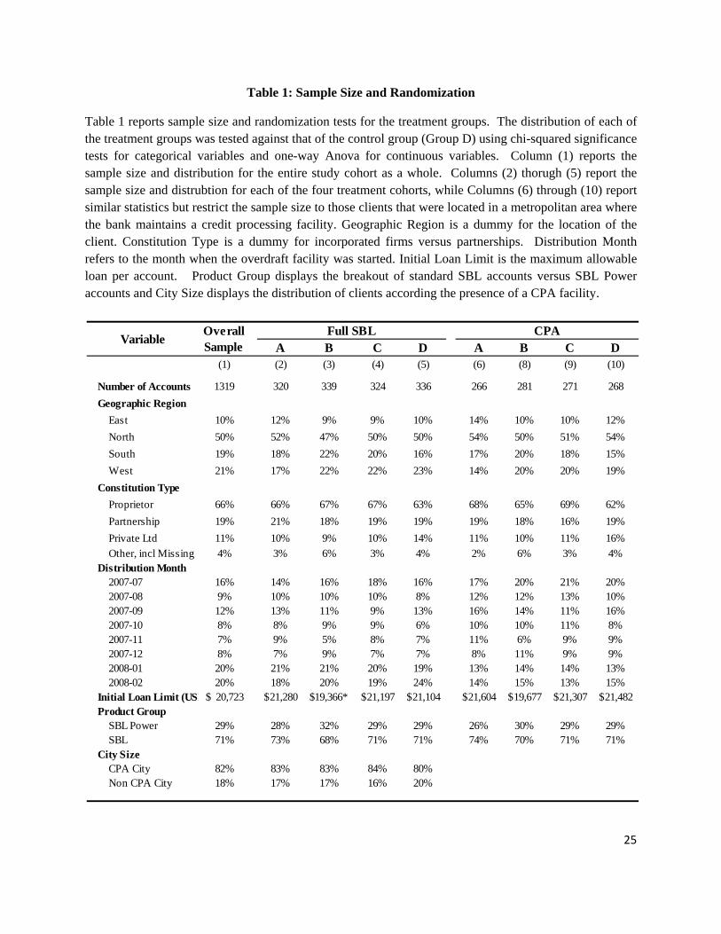
Table 1 reports sample size and randomization tests for the treatment groups. The distribution of each of the treatment groups was tested against that of the control group (Group D) using chi-squared significance tests for categorical variables and one-way Anova for continuous variables. Column (1) reports the sample size and distribution for the entire study cohort as a whole. Columns (2) thorugh (5) report the sample size and distrubtion for each of the four treatment cohorts, while Columns (6) through (10) report similar statistics but restrict the sample size to those clients that were located in a metropolitan area where the bank maintains a credit processing facility. Geographic Region is a dummy for the location of the client. Constitution Type is a dummy for incorporated firms versus partnerships. Distribution Month refers to the month when the overdraft facility was started. Initial Loan Limit is the maximum allowable loan per account. Product Group displays the breakout of standard SBL accounts versus SBL Power accounts and City Size displays the distribution of clients according the presence of a CPA facility.

A B C D A B C D(1) (2) (3) (4) (5) (6) (8) (9) (10)

Number of Accounts 1319 320 339 324 336 266 281 271 268

Geographic Region

East 10% 12% 9% 9% 10% 14% 10% 10% 12%

North 50% 52% 47% 50% 50% 54% 50% 51% 54%

South 19% 18% 22% 20% 16% 17% 20% 18% 15%

West 21% 17% 22% 22% 23% 14% 20% 20% 19%

Constitution Type

Proprietor 66% 66% 67% 67% 63% 68% 65% 69% 62%

Partnership 19% 21% 18% 19% 19% 19% 18% 16% 19%

Private Ltd 11% 10% 9% 10% 14% 11% 10% 11% 16%

Other, incl Missing 4% 3% 6% 3% 4% 2% 6% 3% 4%Distribution Month

2007-07 16% 14% 16% 18% 16% 17% 20% 21% 20%2007-08 9% 10% 10% 10% 8% 12% 12% 13% 10%2007-09 12% 13% 11% 9% 13% 16% 14% 11% 16%2007-10 8% 8% 9% 9% 6% 10% 10% 11% 8%2007-11 7% 9% 5% 8% 7% 11% 6% 9% 9%2007-12 8% 7% 9% 7% 7% 8% 11% 9% 9%2008-01 20% 21% 21% 20% 19% 13% 14% 14% 13%2008-02 20% 18% 20% 19% 24% 14% 15% 13% 15%

Initial Loan Limit (USD 20,723$ 21,280$ $19,366* 21,197$ 21,104$ 21,604$ 19,677$ 21,307$ 21,482$ Product Group

SBL Power 29% 28% 32% 29% 29% 26% 30% 29% 29%SBL 71% 73% 68% 71% 71% 74% 70% 71% 71%

City SizeCPA City 82% 83% 83% 84% 80%Non CPA City 18% 17% 17% 16% 20%

VariableFull SBL CPAOverall

Sample

     

26 

 

Table 2: Descriptive Statistics

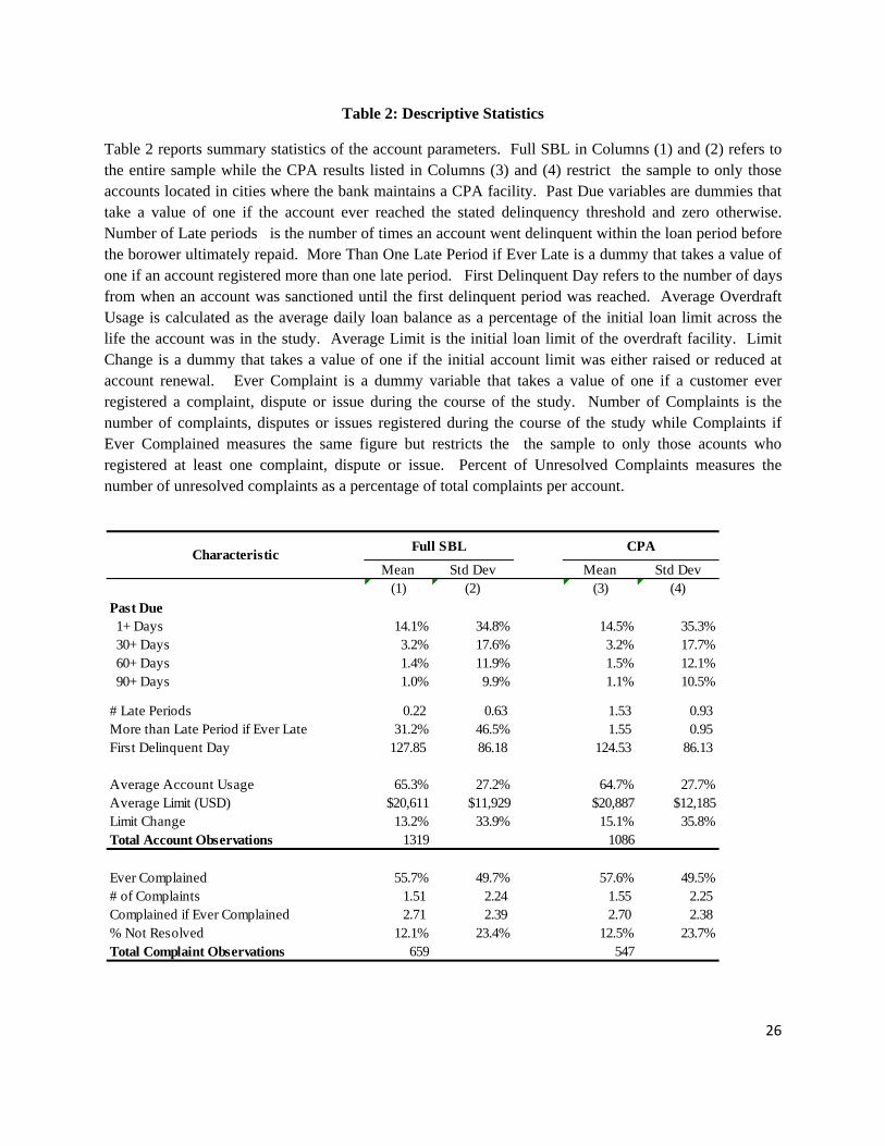
Table 2 reports summary statistics of the account parameters. Full SBL in Columns (1) and (2) refers to the entire sample while the CPA results listed in Columns (3) and (4) restrict the sample to only those accounts located in cities where the bank maintains a CPA facility. Past Due variables are dummies that take a value of one if the account ever reached the stated delinquency threshold and zero otherwise. Number of Late periods is the number of times an account went delinquent within the loan period before the borower ultimately repaid. More Than One Late Period if Ever Late is a dummy that takes a value of one if an account registered more than one late period. First Delinquent Day refers to the number of days from when an account was sanctioned until the first delinquent period was reached. Average Overdraft Usage is calculated as the average daily loan balance as a percentage of the initial loan limit across the life the account was in the study. Average Limit is the initial loan limit of the overdraft facility. Limit Change is a dummy that takes a value of one if the initial account limit was either raised or reduced at account renewal. Ever Complaint is a dummy variable that takes a value of one if a customer ever registered a complaint, dispute or issue during the course of the study. Number of Complaints is the number of complaints, disputes or issues registered during the course of the study while Complaints if Ever Complained measures the same figure but restricts the the sample to only those acounts who registered at least one complaint, dispute or issue. Percent of Unresolved Complaints measures the number of unresolved complaints as a percentage of total complaints per account.

Mean Std Dev Mean Std Dev(1) (2) (3) (4)

14.1% 34.8% 14.5% 35.3%3.2% 17.6% 3.2% 17.7%1.4% 11.9% 1.5% 12.1%1.0% 9.9% 1.1% 10.5%

# Late Periods 0.22 0.63 1.53 0.93 More than Late Period if Ever Late 31.2% 46.5% 1.55 0.95 First Delinquent Day 127.85 86.18 124.53 86.13

65.3% 27.2% 64.7% 27.7%$20,611 $11,929 $20,887 $12,185

Limit Change 13.2% 33.9% 15.1% 35.8%1319 1086

Ever Complained 55.7% 49.7% 57.6% 49.5%# of Complaints 1.51 2.24 1.55 2.25 Complained if Ever Complained 2.71 2.39 2.70 2.38 % Not Resolved 12.1% 23.4% 12.5% 23.7%

659 547

Characteristic

Past Due

Total Account Observations

Full SBL CPA

60+ Days 90+ Days

1+ Days 30+ Days

Average Account UsageAverage Limit (USD)

Total Complaint Observations

     

27 

 

Table 3: OLS Regressions of Deliquency Outcomes on Treatment Groups

Table 3 reports summary data from the OLS regressions of delinquency variables on treatment dummies representing Groups A, B and C and a host of control variables. Treatment Group D serves as the control. Number of Late payments is the number of times an account went delinquent within the loan period before the borrower ultimately repaid. More than one late period is a dummy that takes a value of one if an account registered more than one late period conditional of having at least one late period. 90+ is a dummy that takes the value of one if the account was ever 90+ days delinquent and zero otherwise. SBL Power Product is a dummy that takes a value of one for power product account types while loan limit is the log of the maximum allowable loan provided per account. Large city is a dummy variable that takes a value of one for accounts that are located in metropolitan areas where the bank maintains a credit processing agency. For each dependent variable, two specifications are reported. The first utilizes the entire sample while second restricts the sample to include only accounts located in CPA cities. For the latter specification the dummy variable for large city is ommitted. All regressions include fixed effect controls for 4 different geographic regions, 8 different disbursement months of the SBL product and 6 different types of incorporation of the banking client. R-squared and sample size are reported at the bottom of the table and robust standard errors for all coefficients are reported in parentheses. The symbols ***,**,* indicate significance levels of 1%, 5% and 10%, respectively.

 

Full SBL CPA Full SBL CPA Full SBL CPA

(1) (2) (3) (4) (5) (6)

TreatmentA -0.0912* -0.0939 -0.217** -0.267** 0.00721 0.00903

(0.0513) (0.0577) (0.105) (0.109) (0.00765) (0.00940)

B -0.101** -0.109* -0.245** -0.287** 0.00213 -0.000471

(0.0512) (0.0590) (0.0954) (0.111) (0.00664) (0.00743)

C -0.0643 -0.0519 -0.0724 -0.0470 0.00656 0.00775

(0.0533) (0.0625) (0.0996) (0.114) (0.00754) (0.00918)

SBL Power Product 0.170*** 0.179*** 0.164 0.126 0.00685 0.00508

(0.0512) (0.0577) (0.104) (0.115) (0.00832) (0.00969)

Loan Limit 0.0469 0.0640 -0.0122 -0.0475 -0.00487 -0.00709

(0.0370) (0.0417) (0.0964) (0.106) (0.00837) (0.00982)

Large City 0.0272 0.0945 0.00862

(0.0492) (0.121) (0.00825)

Constant -0.794 -0.560 0.591 1.182 0.0574 0.102

(0.534) (0.578) (1.319) (1.467) (0.122) (0.138)

N 1,319 1,086 186 158 1,319 1,086

R-Squared 0.031 0.034 0.114 0.143 0.014 0.016

90+ DaysNumber of Late

PeriodsMore than One Late period if Ever Late

     

28 

 

Table 4: OLS Regressions of Deliquency Outcomes on Pooled Treatment Groups

Table 4 reports summary data from OLS regressions of delinquency variables on a dummy representing treatment Groups A and B combined. Treatment Groups C and D serve as the control group. We also include the same control variables as in Table 2. 90+ is a dummy that takes the value of one if the account was ever 90+ days delinquent and zero otherwise. Number of Late periods is the number of times an account went delinquent within the loan period before the borrower ultimately repaid. More than one late period is a dummy that takes a value of one if an account registered more than one late period conditional of having at least one late period. SBL Power Product is a dummy that takes a value of one for power product account types while loan limit is the log of the maximum allowable loan provided per account. Large city is a dummy variable that takes a value of one for accounts that are located in metropolitan areas where the bank maintains a credit processing agency. For each dependent variable, two specifications are reported. The first utilizes the entire sample while second restricts the sample to include only accounts located in CPA cities. For the latter specification the dummy variable for large city is ommitted. All regressions also includefixed effect controls for 4 different geographic regions, 8 different disbursement months of the SBL product and 6 different types of incorporation of the banking client. R-squared and sample size are reported at the bottom of the table and robust standard errors for all coefficients are reported in parentheses. The symbols ***,**,* indicate significance levels of 1%, 5% and 10%, respectively.

  

Full SBL CPA Full SBL CPA Full SBL CPA

(1) (2) (3) (4) (5) (6)

Group A & B Dummy -0.0645* -0.0754* -0.198*** -0.253*** 0.00136 0.000256

(0.0350) (0.0396) (0.0693) (0.0756) (0.00561) (0.00659)

SBL Power Product 0.170*** 0.179*** 0.176* 0.135 0.00687 0.00507

(0.0512) (0.0579) (0.102) (0.112) (0.00832) (0.00971)

Loan Limit 0.0464 0.0643 -0.00430 -0.0413 -0.00463 -0.00667

(0.0369) (0.0415) (0.0948) (0.103) (0.00825) (0.00970)

Large City 0.0251 0.0877 0.00874

(0.0492) (0.121) (0.00827)

Constant -0.810 -0.594 0.451 1.098 0.0571 0.0984

(0.536) (0.581) (1.293) (1.427) (0.122) (0.139)

N 1,319 1,086 186 158 1,319 1,086

R-Squared 0.030 0.033 0.110 0.142 0.013 0.014

90+ DaysNumber of Late

PeriodsMore than One Late period if Ever Late

     

29 

 

Table 5: OLS Regressions of Account Behavior Variables on Treatment Groups

Table 5 reports summary data from the OLS regressions of account behavior variables on treatment dummies representing Groups A, B and C. Treatment Group D serves as the control. First Delinquent Day refers to the number of days from when an account was sanctioned until the first delinquent period was reached. Limit Change is a dummy that takes a value of one if the initial account limit was either raised or reduced at account renewal. Category A is dummy that indicates whether accounts were classified with the lowest credit risk at account renewal. Average Overdraft Usage is calculated as the average daily loan balance as a percentage of the initial loan limit for the duration the account was in the study. SBL Power Product is a dummy variable that takes a value of one for power product account types while loan limit is the log of the maximum allowable loan provided per account. Large city is a dummy variable that takes a value of one for accounts that are located in metropolitan areas where the bank maintains a credit processing agency. For each dependent variable, two specifications are reported. The first utilizes the entire sample while second restricts the sample to include only accounts located in CPA cities. For the latter specification the dummy variable for large city is ommitted. All regressions include fixed effect controls for 4 different geographic regions, 8 different disbursement months of the SBL product and 6 different types of incorporation of the banking client. R-squared and sample size are reported at the bottom of the table and robust standard errors for all coefficients are reported in parentheses. The symbols ***,**,* indicate significance levels of 1%, 5% and 10%, respectively.

 

Full SBL CPA Full SBL CPA Full SBL CPA Full SBL CPA

(1) (2) (3) (4) (5) (6) (7) (8)

TreatmentA 34.89* 38.52* 0.0475* 0.0500* 0.0753** 0.0616 -0.0516** -0.0582**

(18.85) (20.37) (0.0251) (0.0292) (0.0371) (0.0412) (0.0212) (0.0239)

B 23.73 25.89 0.0126 0.0160 0.0715** 0.0682* -0.0281 -0.0390*

(16.49) (18.86) (0.0232) (0.0272) (0.0363) (0.0403) (0.0203) (0.0228)

C 26.69 18.27 0.0224 0.0255 0.0141 0.0167 -0.00382 -0.0159

(18.44) (20.12) (0.0241) (0.0283) (0.0362) (0.0403) (0.0208) (0.0233)

SBL Power Product -30.05* -22.13 -0.235*** -0.264*** -0.0581 -0.0625 0.0177 0.00705

(17.47) (19.36) (0.0239) (0.0276) (0.0368) (0.0409) (0.0212) (0.0241)

Loan Limit -16.34 -10.40 -0.0877*** -0.0881*** 0.0471 0.0580 0.00806 0.0140

(15.78) (16.98) (0.0239) (0.0275) (0.0339) (0.0368) (0.0190) (0.0213)

Large City 11.21 -0.0126 -0.0562 -0.0714***

(24.39) (0.0193) (0.0399) (0.0226)

Constant 340.2 261.5 1.404*** 1.165*** -0.0536 0.00925 0.550* 0.364

(226.6) (239.9) (0.371) (0.387) (0.527) (0.515) (0.294) (0.300)

N 186 158 1,319 1,086 1,319 1,086 1,319 1,086

R-Squared 0.155 0.177 0.148 0.152 0.132 0.127 0.041 0.042

Average Overdraft Usage

First Delinquent Day Limit Change Category A

     

30 

 

Table 6: OLS Regressions of Account Behavior Variables on Pooled Treatment Groups

Table 6 reports summary data from OLS regressions of account behavior on a dummy representing treatment Groups A and B combined. Treatment Groups C and D serve as the control group. We also include the same comtrol variables as in Table 4. First Delinquent Day refers to the number of days from when an account was sanctioned until the first delinquent period was reached, thus restricting the sample to delinquent accounts only. Limit Change is a dummy that takes a value of one if the initial account limit was either raised or reduced at account renewal. Category A is dummy that indicates whether accounts were classified with the lowest credit risk at account renewal. Average Overdraft Usage is calculated as the average daily loan balance as a percentage of the initial loan limit for the duration the account was in the study. SBL Power Product is a dummy variable that takes a value of one for power product account types while loan limit is the log of the maximum allowable loan provided per account. Large city is a dummy variable that takes a value of one for accounts that are located in metropolitan areas where the bank maintains a credit processing agency. For each dependent variable, two specifications are reported. The first utilizes the entire sample while second restricts the sample to include only accounts located in CPA cities. For the latter specification the dummy variable for large city is ommitted. All regressions include fixed effect controls for 4 different geographic regions, 8 different disbursement months of the SBL product and 6 different types of incorporation of the banking client. R-squared and sample size are reported at the bottom of the table and robust standard errors for all coefficients are reported in parentheses. The symbols ***,**,* indicate significance levels of 1%, 5% and 10%, respectively.

Full SBL CPA Full SBL CPA Full SBL CPA Full SBL CPA

(1) (2) (3) (4) (5) (6) (7) (8)

Group A&B Dummy 16.30 23.41* 0.0185 0.0198 0.0664** 0.0566** -0.0376** -0.0403**

(12.63) (13.15) (0.0174) (0.0202) (0.0260) (0.0286) (0.0148) (0.0167)

SBL Power Product -33.48** -25.15 -0.235*** -0.264*** -0.0581 -0.0627 0.0177 0.00709

(16.82) (18.20) (0.0239) (0.0276) (0.0368) (0.0409) (0.0212) (0.0241)

Loan Limit -19.25 -12.48 -0.0863*** -0.0867*** 0.0474 0.0578 0.00726 0.0132

(15.37) (16.33) (0.0239) (0.0276) (0.0338) (0.0367) (0.0191) (0.0213)

Large City 15.21 -0.0125 -0.0558 -0.0711***

(24.17) (0.0193) (0.0398) (0.0226)

Constant 384.3* 293.6 1.397*** 1.151*** -0.0520 0.0215 0.557* 0.371

(219.0) (232.2) (0.372) (0.385) (0.527) (0.514) (0.295) (0.300)

N 186 158 1,319 1,086 1,319 1,086 1,319 1,086

R-Squared 0.142 0.169 0.146 0.150 0.132 0.127 0.040 0.041

Average Overdraft Usage

First Delinquent Day Limit Change Category A

     

31 

 

Table 7: OLS Regressions of Delinquency Outcomes and Account Behavior Variables on Caller Adjusted Treatment Groups

Table 7 reports summary data from the OLS regressions of delinquency outcomes and account behavior variables on treatment dummies representing Groups A, B and C. Callers in Treatment Group B who received 50% or more calls from a single caller were recoded to be included in Treatment Group A. Treatment Group D serves as the control. We also include the same comtrol variables as in Table 4. First Delinquent Day refers to the number of days from when an account was sanctioned until the first delinquent period was reached, thus restricting the sample to delinquent accounts only. Limit Change is a dummy that takes a value of one if the initial account limit was either raised or reduced at account renewal. Category A is dummy that indicates whether accounts were classified with the lowest credit risk at account renewal. Average Overdraft Usage is calculated as the average daily loan balance as a percentage of the initial loan limit for the duration the account was in the study. SBL Power Product is a dummy variable that takes a value of one for power product account types while loan limit is the log of the maximum allowable loan provided per account. Large city is a dummy variable that takes a value of one for accounts that are located in metropolitan areas where the bank maintains a credit processing agency. All regressions include fixed effect controls for 4 different geographic regions, 8 different disbursement months of the SBL product and 6 different types of incorporation of the banking client. R-squared and sample size are reported at the bottom of the table and robust standard errors for all coefficients are reported in parentheses. The symbols ***,**,* indicate significance levels of 1%, 5% and 10%, respectively.

Number of Late Periods

More than One Late

period if Ever Late

90+ Days Late

First Delinquent

Day

Limit Change

Category A

Average Overdraft

Usage

Full SBL Full SBL Full SBL Full SBL Full SBL Full SBL Full SBL

(1) (2) (3) (4) (5) (6) (7)

Caller Share Adj. TreatA -0.101** -0.225** 0.00616 37.00** 0.0428* 0.0774** -0.0487**

(0.0504) (0.105) (0.00732) (18.67) (0.0243) (0.0364) (0.0206)

B -0.0905* -0.239** 0.00291 21.69 0.0153 0.0689* -0.0297

(0.0523) (0.0958) (0.00694) (16.61) (0.0237) (0.0371) (0.0207)

C -0.0642 -0.0728 0.00657 26.80 0.0224 0.0141 -0.00385

(0.0533) (0.0996) (0.00754) (18.44) (0.0241) (0.0362) (0.0208)

SBL Power Product 0.170*** 0.164 0.00685 -30.49* -0.235*** -0.0581 0.0177

(0.0512) (0.104) (0.00832) (17.45) (0.0239) (0.0368) (0.0212)

Loan Limit 0.0477 -0.0123 -0.00484 -16.39 -0.0877*** 0.0469 0.00805

(0.0370) (0.0963) (0.00838) (15.75) (0.0239) (0.0339) (0.0191)

Large City 0.0271 0.0950 0.00854 10.47 -0.0131 -0.0562 -0.0711***

(0.0492) (0.122) (0.00822) (24.40) (0.0193) (0.0399) (0.0226)

Constant -0.800 0.259 0.0568 345.5 1.401*** -0.0521 0.552*

(0.534) (1.351) (0.122) (229.0) (0.371) (0.527) (0.295)

N 1,319 186 1,319 186 1,319 1,319 1,319

R-Squared 0.031 0.113 0.014 0.157 0.147 0.133 0.041

     

32 

 

Table 8: OLS Regressions of Monitoring Reachability on Treatment Groups

Table 8 reports summary data from the OLS regressions of survey response variables on a dummy representing treatment Group A. Treatment Group B serves as the control group. Percent Reachable Overall refers is the percent of all calls from the relationship manager in which the client was successfully contacted. Percent Reachable Monitoring 1 is the percent of calls in which the client was reached during the first monitoring call of the month. Percent Reachable Monitoring 2 refers to the percents of calls in which the client was reached during the second monitoring call of the month. SBL Power Product is a dummy variable that takes a value of one for power product account types while loan limit is the log of the maximum allowable loan provided per account. Large city is a dummy variable that takes a value of one for accounts that are located in metropolitan areas where the bank maintains a credit processing agency. For each dependent variable, two specifications are reported. The first utilizes the entire sample while second restricts the sample to include only accounts located in CPA cities. For the latter specification the dummy variable for large city is ommitted. All regressions include fixed effect controls for 4 different geographic regions, 8 different disbursement months of the SBL product and 6 different types of incorporation of the banking client. R-squared and sample size are reported at the bottom of the table and robust standard errors for all coefficients are reported in parentheses. The symbols ***,**,* indicate significance levels of 1%, 5% and 10%, respectively.

 

Full SBL CPA Full SBL CPA Full SBL CPA

(1) (2) (3) (4) (5) (6)

Treatment A 0.0161** 0.0154* 0.00991 0.0127 0.0216** 0.0183*

(0.00725) (0.00793) (0.00796) (0.00880) (0.00869) (0.00935)

SBL Power Product -0.0102 -0.0182 -0.0160 -0.0206 -0.00515 -0.0160

(0.0119) (0.0134) (0.0127) (0.0145) (0.0141) (0.0156)

Loan Limit 0.00316 -0.00157 0.00116 -0.00544 0.00555 0.00214

(0.0119) (0.0135) (0.0116) (0.0132) (0.0145) (0.0162)

Large City 0.00740 -0.00509 0.0169

(0.0109) (0.0118) (0.0140)

Constant 0.870*** 0.889*** 0.916*** 0.929*** 0.825*** 0.851***

(0.167) (0.196) (0.161) (0.192) (0.205) (0.234)

N 659 547 659 547 659 547

R-Squared 0.078 0.094 0.065 0.069 0.064 0.083

% Reachable Overall A & B

% Reachable Monitoring 1

A & B

% ReachableMonitoring 2

A & B

     

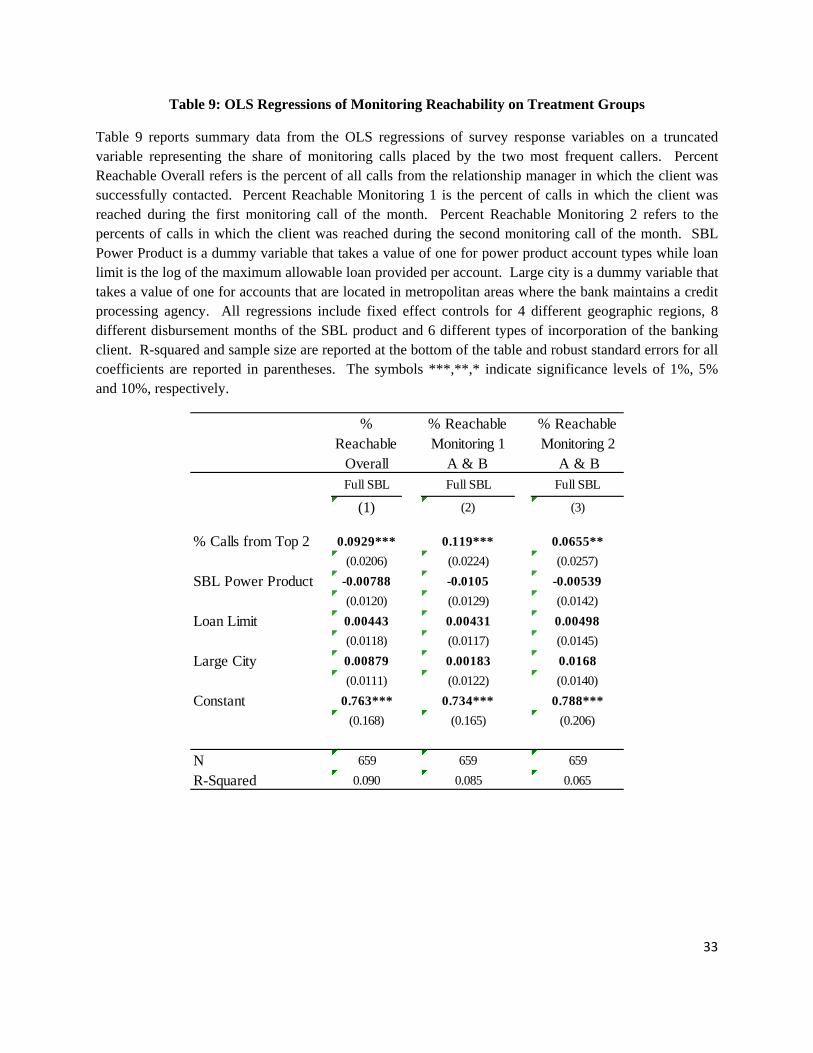
33 

 

Table 9: OLS Regressions of Monitoring Reachability on Treatment Groups

Table 9 reports summary data from the OLS regressions of survey response variables on a truncated variable representing the share of monitoring calls placed by the two most frequent callers. Percent Reachable Overall refers is the percent of all calls from the relationship manager in which the client was successfully contacted. Percent Reachable Monitoring 1 is the percent of calls in which the client was reached during the first monitoring call of the month. Percent Reachable Monitoring 2 refers to the percents of calls in which the client was reached during the second monitoring call of the month. SBL Power Product is a dummy variable that takes a value of one for power product account types while loan limit is the log of the maximum allowable loan provided per account. Large city is a dummy variable that takes a value of one for accounts that are located in metropolitan areas where the bank maintains a credit processing agency. All regressions include fixed effect controls for 4 different geographic regions, 8 different disbursement months of the SBL product and 6 different types of incorporation of the banking client. R-squared and sample size are reported at the bottom of the table and robust standard errors for all coefficients are reported in parentheses. The symbols ***,**,* indicate significance levels of 1%, 5% and 10%, respectively.

% Reachable

Overall

% Reachable Monitoring 1

A & B

% ReachableMonitoring 2

A & BFull SBL Full SBL Full SBL

(1) (2) (3)

% Calls from Top 2 0.0929*** 0.119*** 0.0655**

(0.0206) (0.0224) (0.0257)

SBL Power Product -0.00788 -0.0105 -0.00539

(0.0120) (0.0129) (0.0142)

Loan Limit 0.00443 0.00431 0.00498

(0.0118) (0.0117) (0.0145)

Large City 0.00879 0.00183 0.0168

(0.0111) (0.0122) (0.0140)

Constant 0.763*** 0.734*** 0.788***

(0.168) (0.165) (0.206)

N 659 659 659

R-Squared 0.090 0.085 0.065

     

34 

 

Table 10: OLS Regressions of Customer Complaint Outcomes on Treatment Group A

Table 10 reports summary data from the OLS regressions of customer complaint outcomes on a dummy representing treatment Group A. Treatment Group B serves as the control group. The data is derived from the records of the bimonthly monitoring calls conducted during the study period and the sample size is restricted to clients in Group A or Group B, as they were the only treatment groups whose complaints were recorded. Ever Complaint is a dummy variable that takes a value of one if a customer ever registered a complaint, dispute or issue during the course of the study. Number of Complaints is the number of complaints, disputes or issues registered during the course of the study while Complaints if Ever Complained measures the same figure but restricts the the sample to only those acounts who registered at least one complaint, dispute or issue. Percent of Unresolved Complaints measures the number of unresolved complaints as a percentage of total complaints per account. SBL Power Product is a dummy variable that takes a value of one for power product account types while loan limit is the log of the maximum allowable loan provided per account. Large city is a dummy variable that takes a value of one for accounts that are located in metropolitan areas where the bank maintains a credit processing agency. All regressions include fixed effect controls for 4 different geographic regions, 8 different disbursement months of the SBL product and 6 different types of incorporation of the banking client. R-squared and sample size are reported at the bottom of the table and robust standard errors for all coefficients are reported in parentheses. The symbols ***,**,* indicate significance levels of 1%, 5% and 10%, respectively.

Ever Complaint

Number of Complaints

Complaints if Ever

Complaint

% of Unresolved Complaints

Full SBL Full SBL Full SBL Full SBL

(1) (2) (3) (4)

Treatment A -0.0822** 0.232 0.661*** 0.0570***

(0.0387) (0.173) (0.240) (0.0183)

SBL Power Product 0.00133 0.224 0.548 0.0109

(0.0550) (0.247) (0.335) (0.0257)

Loan Limit 0.0411 0.0607 -0.355 -0.0265

(0.0513) (0.230) (0.308) (0.0227)

Large City -0.00851 0.0747 0.360 0.0356

(0.0621) (0.278) (0.407) (0.0290)

Constant 0.153 0.00380 5.670 0.346

(0.691) (3.095) (4.172) (0.306)

N 659 659 367 659

R-Squared 0.055 0.062 0.195 0.055

     

35 

 

Table 11: OLS Regressions of Customer Satisfaction Outcomes on Treatment Groups

Table 11 reports summary data from the ordered logit regressions of customer responses to an endline survey in June 2009 that asked about their satisfication with the SBL overdraft product on treatment dummies representing Groups A, B and C. Treatment Group D serves as the control. Loan Size measures customer satisfaction with the size of the limit of the overdraft account. Interest Rates refers to satisfaction with the interest charged on the overdraft product, while Branch Customer service refers to satisfaction with the service provided by bank branch offices. Renewal Process measures customer satisfication with the account renewal process conducted at the end of the first year, while Average Rating refers to satisfaction with the SBL product as a whole. Ever Late is a dummy variable which takes a value of one if the customer ever self-reported making late payments on their overdraft account, and the coefficients shown are marginal effects from a probit regressions. All dependent variables except Ever Late measure customer satisifaction for the listed category on a one to five scale spanning very dissastified to very satisfied. Lower bound (upper bound) imputes the highest satisfaction score to non-responders if they were assigned to the control group (treatment group) and the lowest satisfaction score if they were assigned to one of the three treatment groups (control group). The specifications reported in Columns (2) and (7) estimate a minimum treatment effect by imputing the mean plus (minus) .25 standard deviations for the control group (treatment groups) while Columns (4) and (9) estimate a maximum treatment by imputing the mean minus (plus) .25 standard deviations to the control group (treatment groups). The unadjusted specification does not correct for non-responders. SBL Power Product is a dummy variable that takes a value of one for power product account types while loan limit is the log of the maximum allowable loan provided per account. All regressions include fixed effect controls for 4 different geographic regions, 8 different disbursement months of the SBL product and 6 different types of incorporation of the banking client. Psuedo r-squared and sample size are reported at the bottom of the table and robust standard errors for all coefficients are reported in parentheses. The symbols ***,**,* indicate significance levels of 1%, 5% and 10%, respectively.

     

36 

 

Lower Bound

Mean -.25 SD Unadjusted

Mean +.25 SD

Upper Bound

Lower Bound

Mean -.25 SD Unadjusted

Mean +.25 SD

Upper Bound

(1) (2) (3) (4) (5) (6) (7) (8) (9) (10)

TreatmentA -1.772*** -0.0806 0.145 0.661*** 1.974*** -2.027*** -1.429*** -0.355** -0.0569 1.601***

(0.152) (0.138) (0.176) (0.141) (0.154) (0.155) (0.146) (0.175) (0.137) (0.152)

B -1.715*** -0.481*** 0.0717 0.251* 1.843*** -1.837*** -0.494*** -0.135 0.270* 1.598***

(0.150) (0.140) (0.173) (0.138) (0.151) (0.151) (0.137) (0.171) (0.138) (0.149)

C -1.806*** -0.332** 0.102 0.408*** 1.975*** -1.790*** -0.102 0.0816 0.698*** 1.797***

(0.152) (0.139) (0.177) (0.139) (0.154) (0.153) (0.136) (0.174) (0.141) (0.151)

SBL Power Product -0.159 -0.00997 -0.0270 0.0231 0.107 0.0508 0.112 0.173 0.0991 0.174

(0.145) (0.138) (0.178) (0.138) (0.147) (0.149) (0.137) (0.177) (0.138) (0.146)

Loan Limit 0.0261 0.102 0.138 0.113 0.0932 0.0601 0.0359 0.0602 0.00589 0.0235

(0.130) (0.125) (0.160) (0.126) (0.134) (0.134) (0.125) (0.159) (0.126) (0.133)

CPA Cities 1.383*** -0.244 -0.185 -1.224*** 0.643*** -0.0912 -0.312** -1.668***

(0.184) (0.149) (0.149) (0.186) (0.185) (0.146) (0.148) (0.184)

N 1,319 1,319 868 1,319 1,319 1,319 1,319 863 1,319 1,319

R-Squared 0.0794 0.00692 0.00903 0.00823 0.0826 0.0760 0.0248 0.00872 0.0102 0.0791

Lower Bound

Mean -.25 SD Unadjusted

Mean +.25 SD

Upper Bound

Lower Bound

Mean -.25 SD Unadjusted

Mean +.25 SD

Upper Bound

TreatmentA -1.831*** -0.0710 0.240 0.615*** 2.115*** -1.840*** -0.730*** 0.165 1.124*** 2.069***

(0.154) (0.138) (0.180) (0.141) (0.156) (0.153) (0.140) (0.178) (0.143) (0.155)

B -1.778*** -0.215 0.306* 0.916*** 2.115*** -1.665*** -0.372*** 0.374** 1.480*** 2.059***

(0.152) (0.138) (0.179) (0.141) (0.154) (0.150) (0.137) (0.176) (0.146) (0.153)

C -2.004*** -0.727*** -0.0786 0.200 1.993*** -1.874*** -1.112*** 0.0178 0.759*** 1.979***

(0.155) (0.142) (0.181) (0.139) (0.155) (0.152) (0.143) (0.176) (0.139) (0.153)

SBL Power Product -0.0805 -0.0763 -0.0706 -0.0447 0.0129 0.0124 0.0348 0.158 0.113 0.122

(0.148) (0.138) (0.184) (0.138) (0.150) (0.147) (0.137) (0.181) (0.137) (0.149)

Loan Limit -0.0308 -0.0547 -0.115 -0.0563 -0.0716 0.0112 -0.0318 0.0289 0.0180 0.0104

(0.133) (0.125) (0.164) (0.125) (0.135) (0.133) (0.125) (0.162) (0.125) (0.135)

CPA Cities 1.381*** 0.371** 0.424*** -0.885*** 1.052*** 0.333** -0.119 -1.260***

(0.184) (0.147) (0.147) (0.183) (0.183) (0.146) (0.146) (0.182)

N 1,319 1,319 829 1,319 1,319 1,319 1,319 823 1,319 1,319

R-Squared 0.0882 0.0116 0.0110 0.0143 0.0868 0.0764 0.0178 0.0109 0.022 0.0857

Lower Bound

Mean -.25 SD Unadjusted

Mean +.25 SD

Upper Bound

Lower Bound

Mean -.25 SD Unadjusted

Mean +.25 SD

Upper Bound

TreatmentA -1.957*** -0.651*** -0.0617 0.133 1.917*** 0.568*** 0.0743* -0.178***

(0.156) (0.143) (0.182) (0.140) (0.155) (0.0416) (0.0424) (0.0185)

B -1.767*** -0.0951 0.170 0.672*** 1.954*** 0.549*** 0.0943** -0.171***

(0.153) (0.138) (0.181) (0.142) (0.154) (0.0422) (0.0423) (0.0192)

C -1.937*** -0.408*** -0.0126 0.369*** 1.970*** 0.545*** 0.0533 -0.187***

(0.155) (0.140) (0.182) (0.141) (0.155) (0.0428) (0.0412) (0.0183)

SBL Power Product -0.0510 0.0809 0.186 0.111 0.199 0.0829* 0.0549 0.0250

(0.147) (0.139) (0.185) (0.140) (0.149) (0.0436) (0.0397) (0.0321)

Loan Limit 0.0163 0.0417 0.0797 0.0466 0.0459 0.0158 0.0138 0.0136

(0.132) (0.127) (0.166) (0.127) (0.135) (0.0383) (0.0338) (0.0284)

CPA Cities 1.547*** 0.336** 0.397*** -1.088*** -0.585*** -0.122***

(0.187) (0.149) (0.149) (0.186)

N 1,319 1,319 863 1,319 1,319 1,249 828 1,249

R-Squared 0.0957 0.0126 0.0124 0.0131 0.0866 0.249 0.0295 0.112

Loan Size

Average Rating Ever Late

Branch Customer Service Renewal Process

Interest Rates

     

37 

 

Table 12: OLS Regressions of Customer Satisfaction Outcomes on Pooled Treatment Groups

Table 12 reports summary data from the ordered logit regressions of customer responses to an endline survey in June 2009 that asked about their satisfication with the SBL overdraft product on a dummy representing treatment Groups A and B combined. Treatment Groups C and D serve as the control group. Loan size measures customer satisfaction with the size of the limit of the overdraft account. Interest Rates refers to satisfaction with the interest charged on the overdraft product, while Branch Customer service referst to satisfaction with the service provided by bank branch offices. Renewal Process measures customer satisfication with the account renewal process conducted at the end of the first year, while Average Rating refers to satisfaction with the SBL product as a whole. Ever Late is a dummy variable which takes a value of one if the customer ever self-reported making late payments on their overdraft account and the coefficients shown are marginal effects from a probit regressions. All dependent variables except Ever Late measure customer satisifaction for the listed category on a one to five scale spanning very dissastified to very satisfied. Lower bound (upper bound) imputes the highest satisfaction score to non-responders if they were assigned to the control group (treatment group) and the lowest satisfaction score if they were assigned to one of the three treatment groups (control group). The specifications reported in Columns (2) and (7) estimate a minimum treatment effect by imputing the mean plus (minus) .25 standard deviations for the control group (treatment groups) while Columns (4) and (9) estimate a maximum treatment by imputing the mean minus (plus) .25 standard deviations to the control group (treatment groups). The Unadjusted specification does not correct for non-responders. SBL Power Product is a dummy variable that takes a value of one for power product account types while loan limit is the log of the maximum allowable loan provided per account. All regressions include fixed effect controls for 4 different geographic regions, 8 different disbursement months of the SBL product and 6 different types of incorporation of the banking client. Psuedo r-squared and sample size are reported at the bottom of the table and robust standard errors for all coefficients are reported in parentheses. The symbols ***,**,* indicate significance levels of 1%, 5% and 10%, respectively.

     

38 

 

Lower Bound

Mean -.25 SD Unadjusted

Mean +.25 SD

Upper Bound

Lower Bound

Mean -.25 SD Unadjusted

Mean +.25 SD

Upper Bound

(1) (2) (3) (4) (5) (6) (7) (8) (9) (10)

Group A&B Dummy -1.785*** -0.308*** 0.0580 0.437*** 1.850*** -2.027*** -0.611*** -0.279** 0.154 1.605***

(0.108) (0.0990) (0.124) (0.0994) (0.109) (0.155) (0.0997) (0.124) (0.0982) (0.107)

SBL Power Product -0.0808 0.0118 -0.0290 0.0254 0.0156 0.0508 0.0822 0.168 0.0826 0.128

(0.144) (0.139) (0.177) (0.139) (0.144) (0.149) (0.139) (0.177) (0.139) (0.145)

Loan Limit 0.154 0.123 0.139 0.0983 -0.0404 0.0601 0.0103 0.0546 -0.0145 -0.0403

(0.130) (0.126) (0.160) (0.126) (0.131) (0.134) (0.126) (0.159) (0.126) (0.132)

CPA Cities -0.0881 -0.254* -0.218 0.267 0.643*** -0.358** -0.319** -0.328*

(0.174) (0.149) (0.150) (0.176) (0.185) (0.148) (0.149) (0.174)

N 1,319 1,319 868 1,319 1,319 1,319 1,319 863 1,319 1,319

R-Squared 0.0769 0.00715 0.00883 0.00825 0.0797 0.0923 0.0128 0.00799 0.00496 0.0642

Lower Bound

Mean -.25 SD Unadjusted

Mean +.25 SD

Upper Bound

Lower Bound

Mean -.25 SD Unadjusted

Mean +.25 SD

Upper Bound

Group A&B Dummy -1.831*** -0.229** 0.312** 0.665*** 2.099*** -1.840*** -0.679*** 0.264** 1.144*** 2.069***

(0.154) (0.0991) (0.128) (0.100) (0.113) (0.153) (0.101) (0.125) (0.105) (0.155)

SBL Power Product -0.0805 -0.0530 -0.0710 -0.0581 -0.0516 0.0124 0.0696 0.149 0.0696 0.122

(0.148) (0.139) (0.184) (0.139) (0.148) (0.147) (0.138) (0.180) (0.138) (0.149)

Loan Limit -0.0308 -0.0284 -0.117 -0.0658 -0.170 0.0112 0.0243 0.0161 -0.0310 0.0104

(0.133) (0.126) (0.164) (0.126) (0.133) (0.133) (0.126) (0.161) (0.126) (0.135)

CPA Cities 1.381*** 0.382** 0.420*** 0.410** 1.052*** 0.0897 0.170 -1.260***

(0.184) (0.148) (0.149) (0.174) (0.183) (0.147) (0.147) (0.182)

N 1,319 1,319 829 1,319 1,319 1,319 1,319 823 1,319 1,319

R-Squared 0.0749 0.00687 0.0109 0.0152 0.103 0.0734 0.0132 0.0104 0.028 0.0933

Lower Bound

Mean -.25 SD Unadjusted

Mean +.25 SD

Upper Bound

Lower Bound

Mean -.25 SD Unadjusted

Mean +.25 SD

Upper Bound

Group A&B Dummy -1.957*** -0.361*** 0.0627 0.425*** 1.936*** 0.370*** 0.0522** -0.124***

(0.156) (0.100) (0.130) (0.100) (0.111) (0.0238) (0.0253) (0.0218)

SBL Power Product -0.0510 0.0797 0.180 0.0794 0.0631 0.0569 0.0531 0.0256

(0.147) (0.140) (0.185) (0.140) (0.146) (0.0382) (0.0396) (0.0324)

Loan Limit 0.0163 0.0477 0.0698 0.0212 -0.0822 -0.00241 0.0132 0.0115

(0.132) (0.128) (0.166) (0.128) (0.132) (0.0338) (0.0338) (0.0286)

CPA Cities 1.547*** 0.368** 0.412*** 0.412** -0.316*** -0.136***

(0.187) (0.150) (0.151) (0.177) (0.0502) (0.0422)

N 1,319 1,319 863 1,319 1,319 1,249 828 1,249

R-Squared 0.0866 0.0115 0.0116 0.0131 0.0928 0.215 0.0266 0.0545

Branch Customer Service

Interest Rates

Average Rating Ever Late

Loan Size

Renewal Process