the physical impact of sea level rise in the area of...
TRANSCRIPT
Chapter 4
The Physical Impact of SeaLevel Rise in the Area of
Charleston, South Carolina
Timothy W. Kana, Jacqueline Michel,Miles O. Hayes, and John R. Jensen
INTRODUCTION
This chapter reports on a pilot study to determine the shoreline impact from accelerated rises insea level due to anthropogenic (man induced) factors. The methods developed have been applied to thecoastal city of Charleston, South Carolina, to determine the effects of various accelerated sea level risescenarios for the years 2025 and 2075.
In the last few decades, there have been numerous studies on the trends and rates of both eustatic andlocal sea level changes. Eustatic changes are global in nature due to a general rise of the sea level comparedto local changes for a specific area due to the relative rise or subsidence of the land surface with respect toa stationary, general sea level. There has been an overall rise in sea level of about 40 m (130 ft) since thelast glacial epoch, called the Wisconsin ice age, which ended about 14,000 years ago. From 7,000 to 3,000years ago, sea level along the east coast of the United States rose at a rate of about 0.3 cm (0.1 in) per year(Kraft, 1971). Studies of sea level over the last two centuries have estimated that global sea level is risingat a rate of 0.10-0.12 cm/yr (0.04-0.05 in/yr). For the Charleston case study area, Hicks and others (1978,1983) have estimated that the total sea level rise since 1922 has been 0.25 cm/yr (0.1 in/yr).*
*Based on a global (eustatic) rise of 0. 12 cm/yr (0.05 in/yr) plus local subsidence of 0. 13 cm/yr (0.05 in/yr).
Sea Level Rise Physical Impact in Charleston
For our analysis, the local rate was assumed to be 0.25 cm/yr (0. 10 in/yr), and the eustatic rates used werea baseline of 0.12 cm/yr (0.05 in/yr) and the low, medium, and high scenarios discussed in Chapters 1 and3. These scenarios are outlined in Table 4-1 for the years 2025 and 2075.
This chapter describes the physical responses of coastal land forms in Charleston to accelerated sealevel rise. Three types of response are addressed: shoreline changes due to landward displacement of thewater line after a sea level rise (in some geomorphic settings, where sediment supply is great, the shorelinemay accrete or keep pace with a sea level rise.); storm surges that affect new or higher elevations after a sealevel rise; and groundwater changes caused by the intrusion of seawater to higher levels in aquifers.
The chapter is organized as follows. First, the Charleston case study area is described. Then, in turn,we discuss the methodology used in the study: modeling shoreline changes, mapping methods, historicalshoreline trends, and storm surge and groundwater analyses. Finally, the results and an analysis of themethodology used are presented.
CHARLESTON CASE STUDY AREA
History of Human Development
The first European settlers arrived in Charleston around 1670. Since that time, the peninsula city hasundergone dramatic shoreline changes, predominantly by landfilling of the intertidal zone. Early maps showthat over one-third of the peninsula has been "reclaimed." Much of the landfilling occurred on the southerntip of Charleston, behind a high seawall and promenade, known as the Battery. Many of the buildings onthe lower peninsula are of historic value and play an important role in the area's major industry-tourism.These areas already experience frequent flooding during intense rainstorms and unusually high tides andwould high priority for any protection/mitigation actions to prevent further flooding due to sea level rise.
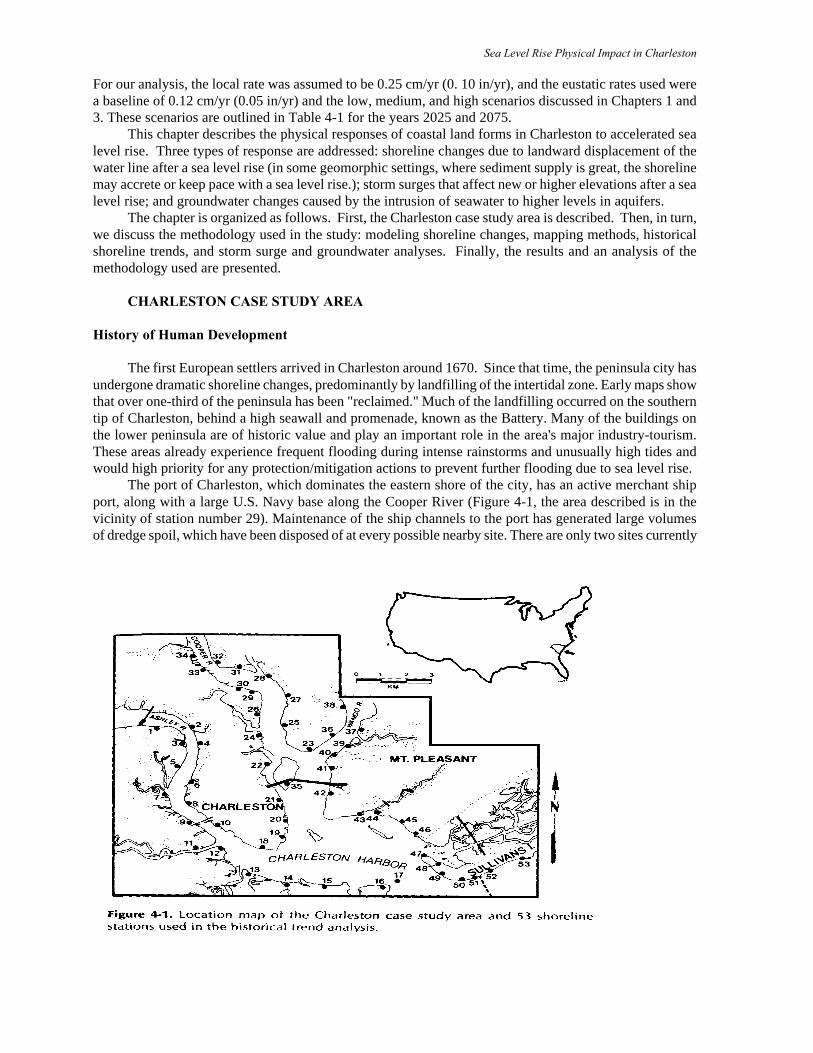
The port of Charleston, which dominates the eastern shore of the city, has an active merchant shipport, along with a large U.S. Navy base along the Cooper River (Figure 4-1, the area described is in thevicinity of station number 29). Maintenance of the ship channels to the port has generated large volumesof dredge spoil, which have been disposed of at every possible nearby site. There are only two sites currently
Sea Level Rise Physical Impact in Charleston
authorized for spoil disposal, and the addition of other sites is unlikely. Plans call for construction of dikesas high as necessary to retain spoil in the designated sites.
The mainland to the east and west of Charleston is primarily residential; much of it is of low density.The trend has been toward slow encroachment on farmland with more intensive development near theharbor, along the Intracoastal Waterway, or on the larger creeks. Sullivans Island and Isle of Palms,developed before World War II, have a large year-round population. These barrier islands northeast ofCharleston Harbor are also the principal recreational beaches for the metropolitan area.
Site Description
The Charleston area has a complex coastal plain morphology which has been significantly alteredby man in the last 100 years (Figure 4-1). The outer shore to the north is composed of geologically young,developed barrier islands (e.g., Sullivans Island) which are relatively flat; elevations typically average lessthan 3 m (10 ft) above mean sea level (MSL) on the islands in the study area. Sheltered by the barrierislands is an extensive, intertidal salt marsh/tidal creek system. At the edge of the marsh/ mainland contact(Figure 4-1, dashed line beginning at station number 46 in Mount Pleasant), there is a break in slope anda distinct change to terrestrial vegetation. Elevations on the lower Charleston peninsula are generally 3 m(10 ft), with small areas up to 5.5 m (18 ft). The study area west of the Ashley River is very flat, withelevations generally about 3 m (10 ft). The Charleston shoreline has a characteristic dendritic drainagepattern typical of drowned coastal plain areas.
The highly populated Charleston peninsula is formed by the junction of three rivers which dischargeinto Charleston Harbor: the Cooper, Ashley, and Wando Rivers (shown in Figure 4-1). The Cooper Riverdominates the discharge into the harbor, with an average flow of 450 m?/s [15,600 ft?/s (cfs)], whichincludes flow from the Santee River (a large river originating in the mountains) diverted for hydroelectricpower in 1942. The diversion has reportedly caused a significant increase in sedimentation in CharlestonHarbor, requiring increased dredging from 400,000 m 3 (525,000 yd3) per year to over 7,500,000 m3
(10,000,000 yd 3) per year (S.C. Water Resources Commission, 1979). Studies have shown that diversionis responsible for 85 percent of the sedimentation in Charleston Harbor (U.S. Army Corps of Engineers,1966). To alleviate this problem, the flow will be rediverted back to the Santee River by 1985, reducingdischarge to one-fifth its present volume. The natural harbor shoreline is dominated by fringing salt marshfrom several meters to over a kilometer wide. As will be shown from the historical shoreline trend data,most of the marshes have accreted since diversion of the Santee into Charleston Harbor.
The entrance to Charleston Harbor has also been modified by the construction of jetties in the 1890sto stabilize the navigation channel. The jetties have caused large-scale changes in sediment transportpatterns, producing up to 300 m (1,000 ft) of deposition along the barrier islands (Sullivans and Isle ofPalms) to the north. Concomitant with accretion north of the harbor, extensive erosion has occurred southof the jetties, including over 500 m (1,700 ft) of erosion along Morris Island (Stephen et. al., 1975). Anotherman-made change in the system is the Intracoastal Waterway, dredged to 4 m (12 ft), which has altered flowpatterns in the marsh behind the barrier islands.
Physical Processes
South Carolina's climate is mild, with an average temperature for the coastal region ranging between10.1EC (50.2E) in December and 27.2EC (81.0EF) in July. An average of 1.4 hurricanes and tropical stormsaffect the coast annually- Winds are somewhat seasonal, with northerly components dominating in fall andwinter and southerly components dominating in spring and summer (Landers, 1970). The tidal rangeincreases considerably from north to south along the state's shoreline, from approximately 1.7 m (5.5 ft) atthe northern border to 2.7 m (8.8 ft) at the southern border. The increasing tidal prism (volume of waterflowing in and out of a harbor or estuary with the movement of the tides) has several effects as one movessouthward along the South Carolina coast: tidal inlets become more frequent and are larger in order to
Sea Level Rise Physical Impact in Charleston
accommodate greater tidal flow, salt marshes are more extensive, and the ebb-tidal deltas (seaward shoalsat inlets) become much larger (Nummedal et al., 1977). Charleston's mean tidal range is 1.6 m (5.2 ft);spring tides average 1.9 m (6.1 ft); and the highest astronomic tides of the year exceed 2.1 m (7.0 ft) (U.S.Department of Commerce, 1981). The spring tidal elevation represents the limit of human developmentbecause the land surface is inundated every 14 days to that elevation, and it is the upper limit of high marshvegetation on which development or any alteration is strictly regulated by South Carolina Coastal ZoneManagement laws (U.S. Department of Commerce, 1979).
The wave climate at Charleston is dependent on offshore swell conditions but is diurnally modified bythe seabreeze/landbreeze cycle typically occurring in the area. The prevailing winds are from the south andwest in these latitudes, but the dominant wind affecting the coastline is from the northeast, originating inextratropical storms travelling parallel to the coast (Finley, 1976). Breaking wave heights along the outerbeaches average approximately 60 cm (2 ft) high in the Charleston area. Predominant wave-energy fluxis directed south along the beaches, accounting for net longshore transport rates of approximately 100,000m3yr (135,000 yd 3/yr) (Kana, 1977).
The relatively large tidal range produces current velocities at all tidal entrances and creeks that oftenexceed 1.5 m/s (5.0 ft/s) (Finley, 1976). With three major tidal rivers within the study site, a diverse set ofestuarine processes influences circulation, flushing, and sedimentation patterns in Charleston Harbor.
The subtropical climate of the southeast produces high weathering rates, which provide large fluxesof sediment to the coastal area. Suspended sediment loads, which dramatically increased in CharlestonHarbor because of diversion of the Santee River, provide significant inputs to the study area and mayaccount for growth of some marsh shorelines. Marshes accrete through the settling of fine-grained sedimenton the marsh surface as cordgrass (Spartina alterniflora) baffles the flow adjacent to tidal creeks. Marshsedimentation has generally been able to keep up with or exceed recent sea level rises along many areas ofthe eastern U.S. shoreline (Ward and Domeracki, 1979).
Hydrogeology
The water table aquifer is composed of surficial sands and clays of Pleistocene age and, in the studyarea, extends to 10-20 m (30-65 ft) below sea level. It is heavily used by the Mount Pleasant and SullivansIsland water districts; both have over 20 wells or well-point systems, each tapping the shallow aquifer.Although the exact position of the freshwater/saltwater interface is unknown, there have been reports ofshallow wells close to shore being moved because of unsuitable water quality. The next geologic unit is theCooper Marl, a calcareous clay, which acts as a confining layer on top of the Santee Limestone-Black Mingoaquifers. These aquifers have not been used for drinking water in the area since about 1950 because ofsaltwater intrusion. The present freshwater/saltwater interface in this aquifer system is thought to be nearSummerville, about 40 km (25 mi) inland (Drennen Parks, 1983, South Carolina Water ResourcesCommission, personal communication).
The Black Creek aquifer of Late Creataceous age is an important water source. Although there isno saltwater currently in the Black Creek aquifer in the study area, the U.S. Geological Survey (USGS) hasmeasured chloride contents of 390-534 mg/l in the lower half of the aquifer on Kiawah and SeabrookIslands, about 30 km (20 mi) to the southwest. The position of the freshwater/saltwater interface in theBlack Creek offshore of Charleston is unknown. The deepest aquifer used in Charleston is the MiddendorfFormation; deep wells down to 700 m (2,200 ft) have not encountered saltwater in the study area. However,on Kiawah and Seabrook Islands, freshwater (62-160 mg/l chloride) was found to 700 m (2,200 ft), andsaline water (1,440 mg/l chloride) was encountered at 790 m (2,400 ft).
The main users of groundwater are the municipalities of Mount Pleasant, Sullivans Island, and Isleof Palms, which use several million gallons per day. Groundwater demand is expected to grow rapidly, asthese areas are projected to experience rapid population growth. The city of Charleston uses surface waterand services the peninsula and west Ashley areas. The present position of the freshwater/saltwater interfacefor the shallow and deep aquifers is unknown, except 30 km (20 mi) to the southwest, and the middle aquifer
Sea Level Rise Physical Impact in Charleston
is already too salty to use. As water usage increases, saltwater intrusion due to overpumpage alone ispredicted to be a serious problem in the future, eventually resulting in abandonment of the shallow aquiferfor potable water.
MODELING EFFECTS OF SEA LEVEL RISEShoreline Changes
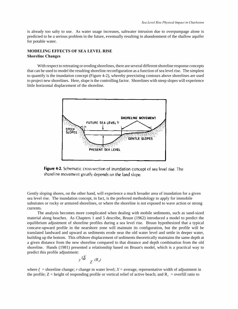
With respect to retreating or eroding shorelines, there are several different shoreline response conceptsthat can be used to model the resulting shoreline reconfiguration as a function of sea level rise. The simplestto quantify is the inundation concept (Figure 4-2), whereby preexisting contours above shorelines are usedto project new shorelines. Here, slope is the controlling factor. Shorelines with steep slopes will experiencelittle horizontal displacement of the shoreline.
Gently sloping shores, on the other hand, will experience a much broader area of inundation for a givensea level rise. The inundation concept, in fact, is the preferred methodology to apply for immobilesubstrates or rocky or armored shorelines, or where the shoreline is not exposed to wave action or strongcurrents.
The analysis becomes more complicated when dealing with mobile sediments, such as sand-sizedmaterial along beaches. As Chapters 1 and 5 describe, Bruun (1962) introduced a model to predict theequilibrium adjustment of shoreline profiles during a sea level rise. Bruun hypothesized that a typicalconcave-upward profile in the nearshore zone will maintain its configuration, but the profile will betranslated landward and upward as sediments erode near the old water level and settle in deeper water,building up the bottom. This offshore displacement of sediments theoretically maintains the same depth ata given distance from the new shoreline compared to that distance and depth combination from the oldshoreline. Hands (1981) presented a relationship based on Bruun's model, which is a practical way topredict this profile adjustment: rX
y = Z
(RA)
where ( = shoreline change; r change in water level; X = average, representative width of adjustment inthe profile; Z = height of responding profile or vertical relief of active beach; and RA = overfill ratio to
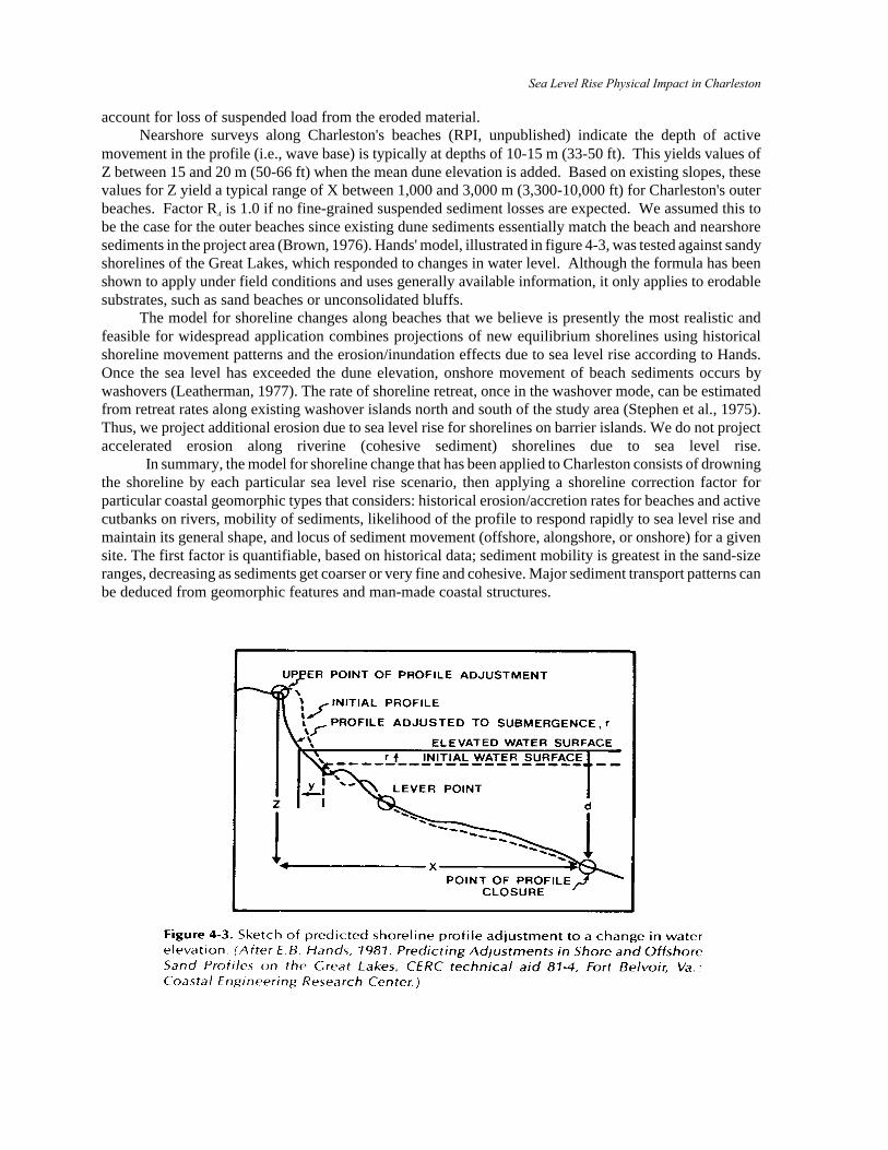
Sea Level Rise Physical Impact in Charleston
account for loss of suspended load from the eroded material.Nearshore surveys along Charleston's beaches (RPI, unpublished) indicate the depth of active
movement in the profile (i.e., wave base) is typically at depths of 10-15 m (33-50 ft). This yields values ofZ between 15 and 20 m (50-66 ft) when the mean dune elevation is added. Based on existing slopes, thesevalues for Z yield a typical range of X between 1,000 and 3,000 m (3,300-10,000 ft) for Charleston's outerbeaches. Factor RA is 1.0 if no fine-grained suspended sediment losses are expected. We assumed this tobe the case for the outer beaches since existing dune sediments essentially match the beach and nearshoresediments in the project area (Brown, 1976). Hands' model, illustrated in figure 4-3, was tested against sandyshorelines of the Great Lakes, which responded to changes in water level. Although the formula has beenshown to apply under field conditions and uses generally available information, it only applies to erodablesubstrates, such as sand beaches or unconsolidated bluffs.
The model for shoreline changes along beaches that we believe is presently the most realistic andfeasible for widespread application combines projections of new equilibrium shorelines using historicalshoreline movement patterns and the erosion/inundation effects due to sea level rise according to Hands.Once the sea level has exceeded the dune elevation, onshore movement of beach sediments occurs bywashovers (Leatherman, 1977). The rate of shoreline retreat, once in the washover mode, can be estimatedfrom retreat rates along existing washover islands north and south of the study area (Stephen et al., 1975).Thus, we project additional erosion due to sea level rise for shorelines on barrier islands. We do not projectaccelerated erosion along riverine (cohesive sediment) shorelines due to sea level rise.
In summary, the model for shoreline change that has been applied to Charleston consists of drowningthe shoreline by each particular sea level rise scenario, then applying a shoreline correction factor forparticular coastal geomorphic types that considers: historical erosion/accretion rates for beaches and activecutbanks on rivers, mobility of sediments, likelihood of the profile to respond rapidly to sea level rise andmaintain its general shape, and locus of sediment movement (offshore, alongshore, or onshore) for a givensite. The first factor is quantifiable, based on historical data; sediment mobility is greatest in the sand-sizeranges, decreasing as sediments get coarser or very fine and cohesive. Major sediment transport patterns canbe deduced from geomorphic features and man-made coastal structures.
Sea Level Rise Physical Impact in Charleston
Storm Surge
The term storm surge refers to any departure from normal water levels due to the action of storms.This can take the form of a set-up or rise in the sea surface due to excess water piling up against the shoreor a set-down if water is removed from the coastal region. For obvious reasons, a super-elevation of coastalwaters is of most concern because of its potential for causing property damage from flooding.
Storm surges are generally reported as a deviation in height from MSL. The magnitude of thisdeviation at any point along the coast is a function of several factors, including: the energy available to moveexcess water toward the coast (wind and waves), the width of the continental shelf, the shape of the basin,and the phase of the normal astronomic tide.
The most widely applied model for predicting open-coast hurricane-surge elevations is the NationalOceanic and Atmospheric Administration's (NOAA) SPLASH [Special Program to List Amplitudes ofSurges from Hurricanes (Jelesnianski, 1972)]. Recently, a model called SLOSH (Sea, Lake, and OverlandSurges from Hurricanes), which "routes" the surge inland, has been developed by NOAA (Jelesnianski andChen, 1984) and is considered the state of the art for inland surge computations. Unfortunately, this modelwas not complete for the Charleston study area at the time the study was undertaken.
Designers and engineers have set standard recurrence intervals such as 1, 10, 25, 50, or 100 yearsto compare flood elevations from one place to another. This can be restated as the percent chance ofoccurrence for a particular flood level in any year. For example, a 10-year flood elevation has a 10 percentchance of occurring each year, whereas a 100-year flood has a 1 percent chance of occurring. The relativeincrease in flood levels from a 10-year to a 100-year storm is generally less than 25 percent (U.S. ArmyCorps of Engineers, 1977). In most regions, this holds true for inland, as well as open-coast, surges. Thegenerally accepted standard for safe design is the 100-year flood level. This is the basis for delineatingflood-prone areas used by the Army Corps of Engineers, NOAA, and the Federal Insurance Administration(FIA).
Two different probability storms were used in the present study to evaluate the effect of sea levelrise on flooding frequency: the 100-year storm and the threshold storm. (Threshold storm is that storm withthe greatest probability of initiating significant damage in the study area.) The 100-year storm elevationsranged from 4. 2 m (14 ft) on the outer beaches to 2.7 m (9 ft) inland. For Charleston, the threshold stormwas selected to be the 10-year storm. It was determined by sequentially raising water levels until significantinundation of developed areas occurred. The 10-year storm elevations ranged from 2.1 m (7 ft) on the outerbeaches to 1.4 m (4.5 ft) inland. Intermediate storm-surges can be selected from frequency curves on thehistorical tidal-storm elevations for Charleston (Myers, 1975).
Groundwater Analyses
Saltwater intrusion is the most common and serious pollutant of fresh groundwater in coastalaquifers. Although many complex mathematical models have been developed to predict saltwater intrusion,a simple concept, the Ghyben-Herzberg principle (Herzberg, 1961), can be used as a conservative estimateof the position of and change in the freshwater/saltwater boundary. The Ghyben-Herzberg principle predicts that the depth of the freshwater/saltwater interface is 40 timesthe elevation of the water table above MSL. Therefore, if the water table is 1 m above MSL, thefreshwater/saltwater interface is predicted to be at 40 m below MSL at that point. For artesian aquifers(aquifers which are confined by overlying, relatively impermeable beds), the freshwater/saltwater interfacecan be predicted by using the elevation of the piezometric surface, which is the artesian pressure or levelof water in the aquifer analogous to the water level in unconfined aquifers. A later section on resultsincludes an explanation of our assumptions regarding the modeling of groundwater impacts from sea levelrise.
Sea Level Rise Physical Impact in Charleston
MAPPING METHODS
The first step required in the analysis was to establish a method for contouring new shorelinepositions and storm surge elevations for each sea level rise scenario. New positions and elevations couldbe plotted by manual interpolation between closest contours on standard USGS topographic maps. Thisprocedure is appropriate for simple shorelines or small geographic areas. However, for the Charleston casestudy, an automated interpolation scheme was necessary for two reasons: first, the 5 ft contour interval onthe existing topographic maps did not provide the necessary detail for accurate interpolation, especiallybetween 0 and 5 ft; and second, there were well over 800 km (500 mi) of shoreline to interpolate.
Topographic maps were made by the translation of map contours using a digital map data base.Computer-generated maps were produced from digital terrain data (point elevations located on ageographical coordinate system). The maps consisted of interpolated contours generated by numericalaveraging within grid squares. For example, the most accurate map would be one that has digital dataplotted every few meters so that contour plotting interpolation would take place over a very small grid cell.Unfortunately, few surveys ever contain "field" data this closely spaced. Also, for practical reasons, gridspacings of a few meters would be inappropriate for a geographical area such as Charleston, which coversover 20 km 2 (75 m 2). Instead, a compromise grid-cell spacing was required that was appropriate to thescale of the map and concentration of original contour data.
Programs using a digital terrain model (DTM) are limited to mapping with grids that fit within adesignated number of rows and columns on the computer matrix. For example, if the largest matrix for aparticular system is 500 rows by 500 columns, map resolution will be proportional to the scale of the map.Each grid unit on a 500 X 500 km map would represent one km2, whereas one unit on a 500 X 500 m mapcould represent one m2. The system used in the present study allowed for a 240 X 256 matrix with a gridcell for the case area of 30 m2(375 ft2 ). This translates to map dimensions of 7.31 X 7.79 km (4.54 X 4.84mi). The study area was approximately 3.2 times these dimensions.
Base Maps
Two types of source map were used to extract topographic/bathymetric control points. First, controlpoints were selected from the USGS 7.5 minute topographic maps at a scale of 1:24,000 with 1.5 m (5 ft)contour intervals. Control points from this source were measured to the nearest foot. The control pointswere obtained by periodically sampling the contour lines and using existing benchmarks. All contours andbenchmarks from -1.8 m (-6 ft) MSL up to +5.8 m (+19 ft) MSL were sampled.
An additional map source covering the city of Charleston (1:2,400 planimetric maps with 1ft contourintervals) was used to supplement the digital topography data. Only benchmark data (no contours) wereused in this data set. Control points from the large-scale maps were digitized at a resolution of 0.03 m (0.1ft), substantially improving the quality of the DTM-computer-generated map, compared with using only datafrom the 1:24,000 scale USGS quadrangles. This procedure is recommended wherever additional, moreaccurate map sources are available.
Digitization
The spatial resolution of the DTM was chosen to be 30 m (100 ft) on the 1:24,000 base map. Theelevation matrices for the study area were generated with dimensions of 240 rows by 256 columns [7.31 X7.79km (4.54 X 4.84mi)] . A total of 3.5 maps was required (2,000-2,500 data points each) to cover theentire project area. A two-phase interpolation algorithm was employed to estimate the elevation values forall 900-m 2 (9,700-ft 2) cells. The first phase performed a quadrant search around each cell in question toensure that control points would be obtained from at least two of the compass directions. A nearest-neighbormethod then automatically selected, from the subset of control points generated initially, the n nearestneighbors to estimate the elevation of each cell. The interpolation was to the nearest 0.03 m (0.1ft), resultingin a DTM with relatively accurate elevation data.
Sea Level Rise Physical Impact in Charleston
Contour maps were generated and overlaid onto the 1:24,000 base map to determine the planimetricand topographic accuracy of the interpolated grid matrix. When discrepancies occurred, additional controlpoints were located and digitized, and a new grid matrix was created by the same interpolation methoddescribed above. This procedure was repeated several times to improve resolution as much as possiblewithin the size limits of each grid cell.
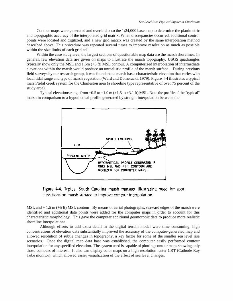
Within the case study area, the largest sections of questionable map data are the marsh shorelines. Ingeneral, few elevation data are given on maps to illustrate the marsh topography. USGS quadranglestypically show only the MSL and 1.5m (+5 ft) MSL contour. A computerized interpolation of intermediateelevations within the marsh would produce an unrealistic profile of the marsh surface. During previousfield surveys by our research group, it was found that a marsh has a characteristic elevation that varies withlocal tidal range and type of marsh vegetation (Ward and Domeracki, 1979). Figure 4-4 illustrates a typicalmarsh/tidal creek system for the Charleston area (a shoreline type representative of over 75 percent of thestudy area).
Typical elevations range from +0.5 to +1.0 m (+1.5 to +3.1 ft) MSL. Note the profile of the "typical"marsh in comparison to a hypothetical profile generated by straight interpolation between the
MSL and + 1.5 m (+5 ft) MSL contour. By means of aerial photographs, seaward edges of the marsh wereidentified and additional data points were added for the computer maps in order to account for thischaracteristic morphology. This gave the computer additional geomorphic data to produce more realisticshoreline interpolations.
Although efforts to add extra detail in the digital terrain model were time consuming, highconcentrations of elevation data substantially improved the accuracy of the computer-generated map andallowed resolution of subtle changes in topography, a key factor for some of the smaller sea level risescenarios. Once the digital map data base was established, the computer easily performed contourinterpolation for any specified elevation. The system used is capable of plotting contour maps showing onlythose contours of interest. It also can display color maps on a high resolution raster CRT (Cathode RayTube monitor), which allowed easier visualization of the effect of sea level changes.
Sea Level Rise Physical Impact in CharlestonComputer-Generated Maps
Contour/bathymetric maps displaying the desired contours and contour intervals were prepared,scaled to overlay the original 1:24,000 scale base map. Various combinations of contours and contourintervals were plotted, depending upon the sea level rise scenario selected. These computer generated mapsbecame the new base maps for final determination of shoreline position using geomorphic data andincreased storm surge elevations. Vertical resolution of contours was to the nearest 0.03 in (0.1 ft), whereasspatial resolution was " 15m (50 ft).
The color CRT allowed viewing various sea level rise scenarios applying the simple inundationconcept. By choosing colors illustrative of water, intertidal, and land areas, it was possible to obtain apreliminary picture of the effect of each sea level scenario. The digital terrain elevation values wereconverted to 8 bit (byte) data ranging from values of 0 to 255. Selected elevation class intervals wereassigned different colors to represent baseline and predicted changes in sea level and storm surge elevations.Although the CRT screen does not offer permanent hard copy for detailed analysis, it can be photographeddirectly for illustrative purposes. This is one of the most useful modern tools for applications of this kind.
HISTORICAL SHORELINE TRENDS
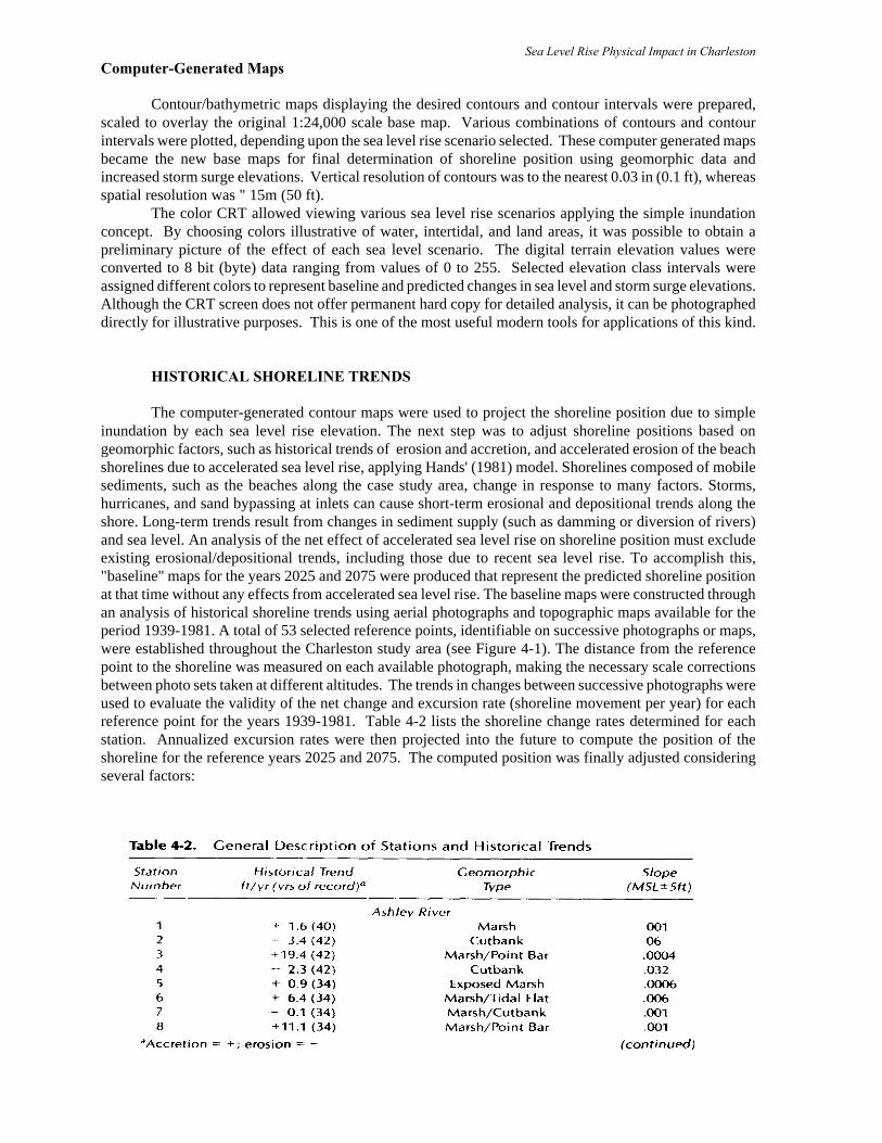
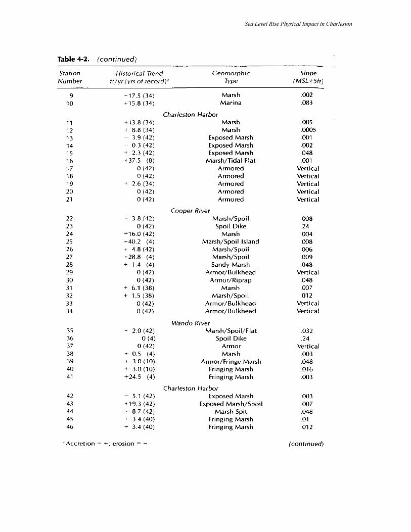
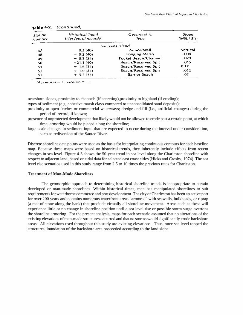
The computer-generated contour maps were used to project the shoreline position due to simpleinundation by each sea level rise elevation. The next step was to adjust shoreline positions based ongeomorphic factors, such as historical trends of erosion and accretion, and accelerated erosion of the beachshorelines due to accelerated sea level rise, applying Hands' (1981) model. Shorelines composed of mobilesediments, such as the beaches along the case study area, change in response to many factors. Storms,hurricanes, and sand bypassing at inlets can cause short-term erosional and depositional trends along theshore. Long-term trends result from changes in sediment supply (such as damming or diversion of rivers)and sea level. An analysis of the net effect of accelerated sea level rise on shoreline position must excludeexisting erosional/depositional trends, including those due to recent sea level rise. To accomplish this,"baseline" maps for the years 2025 and 2075 were produced that represent the predicted shoreline positionat that time without any effects from accelerated sea level rise. The baseline maps were constructed throughan analysis of historical shoreline trends using aerial photographs and topographic maps available for theperiod 1939-1981. A total of 53 selected reference points, identifiable on successive photographs or maps,were established throughout the Charleston study area (see Figure 4-1). The distance from the referencepoint to the shoreline was measured on each available photograph, making the necessary scale correctionsbetween photo sets taken at different altitudes. The trends in changes between successive photographs wereused to evaluate the validity of the net change and excursion rate (shoreline movement per year) for eachreference point for the years 1939-1981. Table 4-2 lists the shoreline change rates determined for eachstation. Annualized excursion rates were then projected into the future to compute the position of theshoreline for the reference years 2025 and 2075. The computed position was finally adjusted consideringseveral factors:
Sea Level Rise Physical Impact in Charleston
Sea Level Rise Physical Impact in Charleston
nearshore slopes, proximity to channels (if accreting),proximity to highland (if eroding); types of sediment (e.g.,cohesive marsh clays compared to unconsolidated sand deposits); proximity to open fetches or commercial waterways; dredge and fill (i.e., artificial changes) during the
period of record, if known;presence of unprotected development that likely would not be allowed to erode past a certain point, at which
time armoring would be placed along the shoreline; large-scale changes in sediment input that are expected to occur during the interval under consideration,
such as rediversion of the Santee River.
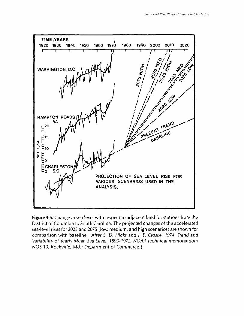
Discrete shoreline data points were used as the basis for interpolating continuous contours for each baselinemap. Because these maps were based on historical trends, they inherently include effects from recentchanges in sea level. Figure 4-5 shows the 50-year trend in sea level along the Charleston shoreline withrespect to adjacent land, based on tidal data for selected east coast cities (Hicks and Crosby, 1974). The sealevel rise scenarios used in this study range from 2.5 to 10 times the previous rates for Charleston.
Treatment of Man-Made Shorelines
The geomorphic approach to determining historical shoreline trends is inappropriate to certaindeveloped or man-made shorelines. Within historical times, man has manipulated shorelines to suitrequirements for waterborne commerce and port development. The city of Charleston has been an active portfor over 200 years and contains numerous waterfront areas "armored" with seawalls, bulkheads, or riprap(a mat of stone along the bank) that preclude virtually all shoreline movement. Areas such as these willexperience little or no change in shoreline position until a sea level rise or possible storm surge overtopsthe shoreline armoring. For the present analysis, maps for each scenario assumed that no alterations of theexisting elevations of man-made structures occurred and that no storms would significantly erode backshoreareas. All elevations used throughout this study are existing elevations. Thus, once sea level topped thestructures, inundation of the backshore area proceeded according to the land slope.
Sea Level Rise Physical Impact in Charleston
Sea Level Rise Physical Impact in Charleston
Treatment of Marsh Shorelines
Shorelines fronted by marshes were treated differently than sand beaches because they do notmaintain an equilibrium profile with sea level changes. Marsh surfaces accrete through the deposition offine-grained, suspended sediment when water flow is baffled by marsh vegetation. Erosion of marshes isa slow process of wave erosion at the seaward edge of the marsh or at cutbanks of meandering streams. Asshown in Table 4-2, most of the marsh stations in Charleston have been accretionary since 1939. However,the rediversion of the Santee River is expected to reduce the sediment input by 85 percent, and the marshesare not likely to continue accreting as in the recent past.
Our analysis did not assume that marsh sedimentation would keep pace with sea level rise in the(low to high) scenarios. Therefore, a sea level rise would result in significant flooding of areas that are nowmarshes. Where marshes exist, there tends to be a critical elevation range for the majority of the deposit.In Charleston, that range is from +0.5 m (1.5 ft) to the highest normal level of tidal inundation, referred toas mean spring high water (MSHW).
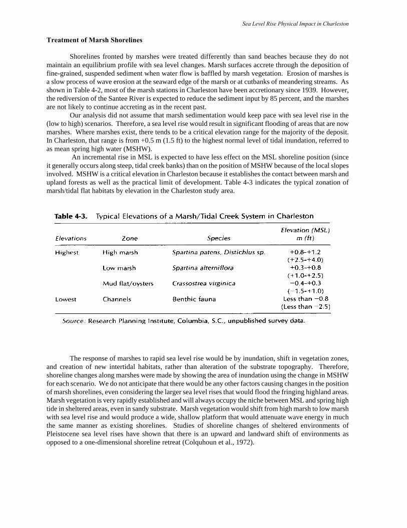
An incremental rise in MSL is expected to have less effect on the MSL shoreline position (sinceit generally occurs along steep, tidal creek banks) than on the position of MSHW because of the local slopesinvolved. MSHW is a critical elevation in Charleston because it establishes the contact between marsh andupland forests as well as the practical limit of development. Table 4-3 indicates the typical zonation ofmarsh/tidal flat habitats by elevation in the Charleston study area.
The response of marshes to rapid sea level rise would be by inundation, shift in vegetation zones,and creation of new intertidal habitats, rather than alteration of the substrate topography. Therefore,shoreline changes along marshes were made by showing the area of inundation using the change in MSHWfor each scenario. We do not anticipate that there would be any other factors causing changes in the positionof marsh shorelines, even considering the larger sea level rises that would flood the fringing highland areas.Marsh vegetation is very rapidly established and will always occupy the niche between MSL and spring hightide in sheltered areas, even in sandy substrate. Marsh vegetation would shift from high marsh to low marshwith sea level rise and would produce a wide, shallow platform that would attenuate wave energy in muchthe same manner as existing shorelines. Studies of shoreline changes of sheltered environments ofPleistocene sea level rises have shown that there is an upward and landward shift of environments asopposed to a one-dimensional shoreline retreat (Colquhoun et al., 1972).
Sea Level Rise Physical Impact in CharlestonDetermination of Shoreline Change
The shoreline position (at mean high spring tide) for each of the 53 stations in the study area wascomputed for all scenarios at the years 2025 and 2075, respectively. Because of the large reduction insediment input anticipated when the Santee River is rediverted, the marshes were assumed to go into a stablephase with no change projected from the historical trends, which are accretionary. The only shorelinechange in the marsh stations for the baseline maps was assumed to be by inundation due to the continuedhistorical rise in sea level at 0.25 cm/yr (0.1 in/yr). The total baseline change in the position of sandyshorelines (station numbers 49-53) for each scenario year included both extrapolation of historical trends(in ft/yr O number of years) and inundation. Discrete station data were used to produce the baseline mapsfor the years 2025 and 2075.
The changes in shoreline location by scenario for each year are estimated as the net change causedby accelerated sea level rise, measured from the baseline for that year, and total change, measured from the1979 USGS 7.5 minute topographic maps. The net and total change included only inundation for marshshorelines. The net change on sandy beaches included inundation and erosion (projection of historicaltrends using Hands' (1981) relationship) due to the higher sea level. After sea level topped the currentelevation of the dunes, the shoreline retreat was projected as a washover process, using averaged rates fromexisting washover islands along the South Carolina coast (as determined by Stephen et al., 1975). The totalchange was a summation of the historical trends and the sea level rise-induced changes. Therefore, ratherthan project the total disappearance of the barrier island, it was assumed that waves would build washoverridges to the spring tidal level for a uniform width which would migrate landward. The appendix tables atthe end of this chapter show predicted shoreline changes for all scenarios and stations, giving a breakdownof the various components contributing to the change.
Example Analysis. As an example, the analysis for one station (52 on Figure 4-1) follows (see alsoappendix). The historical trend at that station for the last 40 years has been +0.3 m (1.0 ft/yr) of accretion.(It is a beach along a recurved spit on Sullivans Island.) To determine the change in the position of theshoreline for the year 2025 without accelerated sea level rise (the baseline position), the yearly depositionalrate was multiplied by 45, equal to 14 m (45 ft) of accretion. Historical sea level rise rates were alsoprojected to the year 2025 to determine the elevation of MSHW at that time, under the baseline scenario,which was a rise of 11 cm (0.4 ft). This placed MSHW for the year 2025 (baseline) at 1.0 m (3.5 ft) abovepresent MSL. Computer-plotted maps of the present and 2025 baseline shoreline positions were overlaidand the change in position measured. For Station 52, there was a change of -6 m (-20 ft) due to inundationalong the existing beach slope. The total change in the 2025 baseline position, compared to the present, wasthe sum of both the historical trend and inundation, which in this case was equal to +7.6 m (+25 ft). Thechange in shoreline position for the 2025 low scenario can be measured from both the present shoreline(called total change) or from the projected baseline position (called net change), which is due solely toaccelerated sea level rise. Net change was determined by summing the inundation component (from thecomparison of contour positions for each MSHW elevation), which was -15 m (-50 ft) for Station 52, anda component for additional erosion due to the higher sea level, using Hands '(1981) model, which was -14m (-45 ft). The total change from the present also included the change from the present due to historicaltrends in erosion or deposition. Thus, the total change for Station 52 under the 2025 low scenario was equalto -21 m (-70 ft), which is the sum of the projected baseline [+8 m (+25 ft)], plus changes due to inundation[-15 m (-50 ft)], plus the effect of accelerated erosion [-14 m (-45 ft)].
Shoreline changes due to inundation were measured at each station directly from the computer-generated contour maps for each sea level rise. The shoreline position was then altered whereappropriate according to historical trends for baseline maps or erosion due to sea level rise on eachscenario map. The shoreline between stations was interpolated using the shoreline type and adjacentstations as guides.
Sea Level Rise Physical Impact in CharlestonSTORM SURGE ANALYSES
The next major impact of sea level rise considered was the alteration of storm surge levels inproportion to the sea level rise scenario. There may be minor factors that would tend to change theincremental rise in storm surge elevations, but these would be dwarfed by the present inaccuracies of inlandsurge modeling. The approach used was to elevate the selected storm surges (10-year and 100-year storms)by an amount equal to the sea level rise scenario. Although this technique is slightly conservative, by notaccounting for displacement of the storm surge inland with sea level rise, there is no available model toestimate what the effects of sea level rise would be on the inland routing of the storm surge.
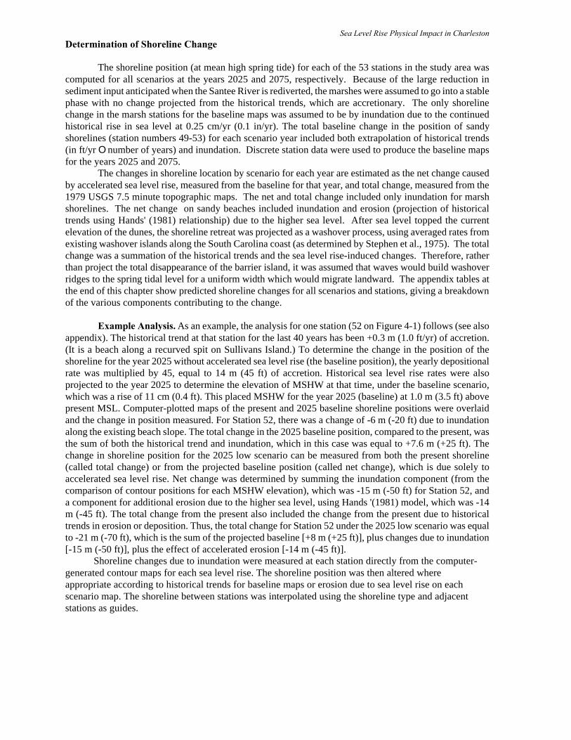
Storm surge elevations for the study area were taken from Federal Emergency Management Agency(FEMA) flood maps. These maps, produced for various Charleston sites since the early 1970s, are the basisfor Federal Flood Insurance rates and zoning and indicate flooding zones and corresponding surge elevationsfor the 100-year event (storm with a probability of 0.01). The 10-year storm elevation (with a probabilityof 0.1) was determined from a summary of storm tide frequencies prepared by Myers (1975) for Charleston(Figure 4-6). This figure shows that for the 10-year storm, total tidal heights would be above 1.5 m (5 ft)MSL.
GROUNDWATER ANALYSES
There have been numerous case studies of saltwater intrusion, which generally occurs from thereversal or reduction of groundwater gradients which causes denser saltwater to displace freshwater or fromthe destruction of natural barriers separating freshwater and saltwater. Many methods have been developed
Sea Level Rise Physical Impact in Charlestonto calculate the position, simulate the motion, and predict the rate of intrusion of the freshwater/saltwaterboundary (Cooper et al., 1964; Mercer et al., 1980; Pinder and Cooper,1970). The most accurate methodsinvolve complex convective-dispersive solute-transport equations, which require specific hydrogeologicalparameters and are difficult to solve. Also, for many coastal aquifers, hydrogeological parameters are notwell known, not even within an order of magnitude.
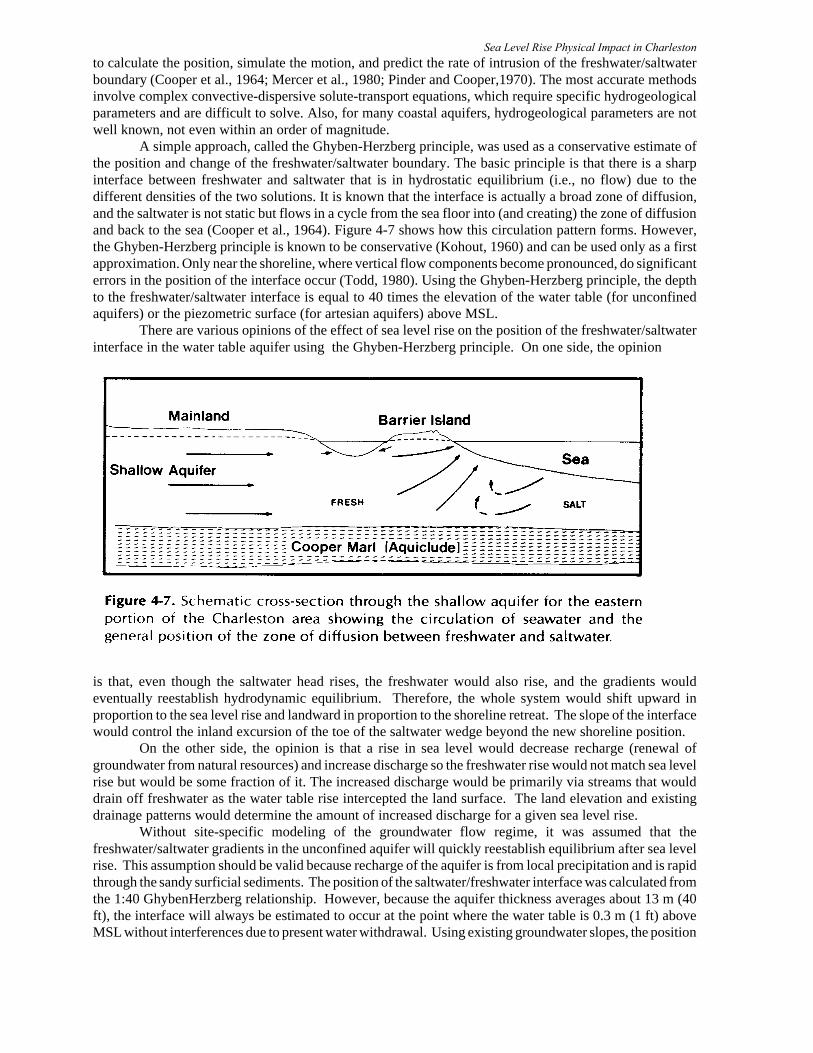
A simple approach, called the Ghyben-Herzberg principle, was used as a conservative estimate ofthe position and change of the freshwater/saltwater boundary. The basic principle is that there is a sharpinterface between freshwater and saltwater that is in hydrostatic equilibrium (i.e., no flow) due to thedifferent densities of the two solutions. It is known that the interface is actually a broad zone of diffusion,and the saltwater is not static but flows in a cycle from the sea floor into (and creating) the zone of diffusionand back to the sea (Cooper et al., 1964). Figure 4-7 shows how this circulation pattern forms. However,the Ghyben-Herzberg principle is known to be conservative (Kohout, 1960) and can be used only as a firstapproximation. Only near the shoreline, where vertical flow components become pronounced, do significanterrors in the position of the interface occur (Todd, 1980). Using the Ghyben-Herzberg principle, the depthto the freshwater/saltwater interface is equal to 40 times the elevation of the water table (for unconfinedaquifers) or the piezometric surface (for artesian aquifers) above MSL.
There are various opinions of the effect of sea level rise on the position of the freshwater/saltwaterinterface in the water table aquifer using the Ghyben-Herzberg principle. On one side, the opinion
is that, even though the saltwater head rises, the freshwater would also rise, and the gradients wouldeventually reestablish hydrodynamic equilibrium. Therefore, the whole system would shift upward inproportion to the sea level rise and landward in proportion to the shoreline retreat. The slope of the interfacewould control the inland excursion of the toe of the saltwater wedge beyond the new shoreline position.
On the other side, the opinion is that a rise in sea level would decrease recharge (renewal ofgroundwater from natural resources) and increase discharge so the freshwater rise would not match sea levelrise but would be some fraction of it. The increased discharge would be primarily via streams that woulddrain off freshwater as the water table rise intercepted the land surface. The land elevation and existingdrainage patterns would determine the amount of increased discharge for a given sea level rise.
Without site-specific modeling of the groundwater flow regime, it was assumed that thefreshwater/saltwater gradients in the unconfined aquifer will quickly reestablish equilibrium after sea levelrise. This assumption should be valid because recharge of the aquifer is from local precipitation and is rapidthrough the sandy surficial sediments. The position of the saltwater/freshwater interface was calculated fromthe 1:40 GhybenHerzberg relationship. However, because the aquifer thickness averages about 13 m (40ft), the interface will always be estimated to occur at the point where the water table is 0.3 m (1 ft) aboveMSL without interferences due to present water withdrawal. Using existing groundwater slopes, the position
Sea Level Rise Physical Impact in Charlestonof the interface was estimated to be at approximately 60m (200ft) inland of the new shoreline position foreach scenario. Thus, for this study, saltwater intrusion after sea level rise can be approximated by the shoreerosion/inundation distance for each scenario. For artesian aquifers, the adjustment in thefreshwater/saltwater interface can be predicted using the Ghyben-Herzberg principle: that is, a 1:40 ratiofor sea level rise to freshwater/saltwater interface rise (Henry,1962). The recharge zone for artesian aquifersis generally far removed from the coast, and there would not be a significant increase in discharge. However,the time lag of saltwater intrusion is very large, as discussed in the next section.
Rates of Saltwater Intrusion
The rates of adjustment of the freshwater/saltwater zone of diffusion in groundwater in response tosea level rise will be different for water table compared to confined aquifers. Although a determination ofthe absolute rates is beyond the scope of this study, there are examples which demonstrate the relative ratesto be expected.
There are many examples of very rapid saltwater contamination of water table aquifers due toman's activities. Large-scale construction of canals in south Florida has resulted in the penetration ofsaltwater into previously fresh areas-an effect somewhat analogous to sea level rise. Dense saltwatergradually replaced fresh groundwater below the canals in several years, including a drought (Parker,1955). The saltwater zone then moved in response to gradients created by heavy pumping in the area. In New Jersey, construction of the Washington Canal in the early 1940s breached the confining layer ofthe shallow aquifer. By the 1980s, saltwater had traveled 8-16 km (5-10 mi) inland (Harold Miesler,1983, USGS, personal communication). There are many other case histories that show that whereshallow aquifers come in direct contact with seawater, saltwater intrusion can occur on a scale of severalto tens of years. The time necessary to reach equilibrium may be much longer and is generallycomplicated by local changes in recharge and discharge.
The rates of adjustment in extensive artesian aquifers will be very slow, especially for the deep,stratified aquifers along the east coast. The USGS is developing a digital technique to model the movementof the altwater/freshwater zone of diffusion during the sea level fluctuations throughout the Pleistoceneepoch (Harold Miesler, 1983, USGS, personal communication). Although the model is still beingdeveloped, they estimate that the time required for stabilization of the zone of diffusion for the New Jerseysections with which they are working is on the order 105 and 106 years.
These calculated time periods are supported by studies done by the USGS on the Atlanticcontinental shelf. Hathaway et al. (1979) reported that low-chlorinity water occurs beneath much of the shelffrom 16 to 120 km (10-75 mi) offshore. The general pattern was described as a freshwater lens overlain bylow-permeability clays, which have a sharp chlorinity gradient increasing toward seawater concentrations.They interpret the freshwater lens as a remnant of fresh groundwater that recharged the shelf sedimentsduring the Pleistocene glacial maximum, when sea level was as much as 100 m (330 ft) lower than present.The impermeable clay has acted as a confining bed, preventing saltwater intrusion during the last floodingof the continental shelf about 8,000 years ago. Hathaway et al. (1979) proposed that the offshore freshwaterlens had played an important role in preventing saltwater intrusion into mainland wellfields. The slow ratesof adjustment in the freshwater/saltwater zone of diffusion is further supported by reports of remnant salinewater that intruded during higher sea level stands into various coastal aquifers (Stringfield, 1966; Wilson,1982).
RESULTS AND DISCUSSION
Smooth shoreline and flood maps for the various baseline and sea level rise scenarios for the years2025 and 2075 were prepared from the digital terrain model and methodology already outlined. Thefollowing results offer a sampling of the changes expected under selected scenarios. A technical report byMichel et al. (1982) contains a more complete data summary.
The first set of maps prepared illustrate existing conditions, giving the location of the 1980 MSL
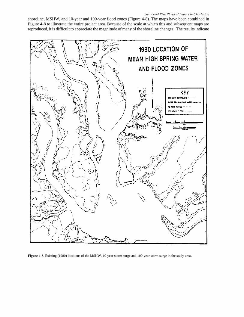
Sea Level Rise Physical Impact in Charlestonshoreline, MSHW, and 10-year and 100-year flood zones (Figure 4-8). The maps have been combined inFigure 4-8 to illustrate the entire project area. Because of the scale at which this and subsequent maps arereproduced, it is difficult to appreciate the magnitude of many of the shoreline changes. The results indicate
Figure 4-8. Existing (1980) locations of the MSHW, 10-year storm surge and 100-year storm surge in the study area.
Sea Level Rise Physical Impact in Charlestonfuture shoreline change is indeed significant under all but the lowest scenarios. At the scale of these maps,a pencil width represents up to 100 m (330 ft) of change, a result that would certainly be of concern to mostshorefront property owners. Despite the complexity of the maps at this scale, major trends are still apparent.
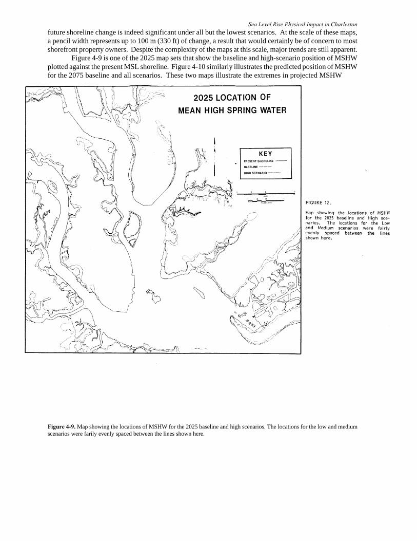
Figure 4-9 is one of the 2025 map sets that show the baseline and high-scenario position of MSHWplotted against the present MSL shoreline. Figure 4-10 similarly illustrates the predicted position of MSHWfor the 2075 baseline and all scenarios. These two maps illustrate the extremes in projected MSHW
Figure 4-9. Map showing the locations of MSHW for the 2025 baseline and high scenarios. The locations for the low and mediumscenarios were farily evenly spaced between the lines shown here.
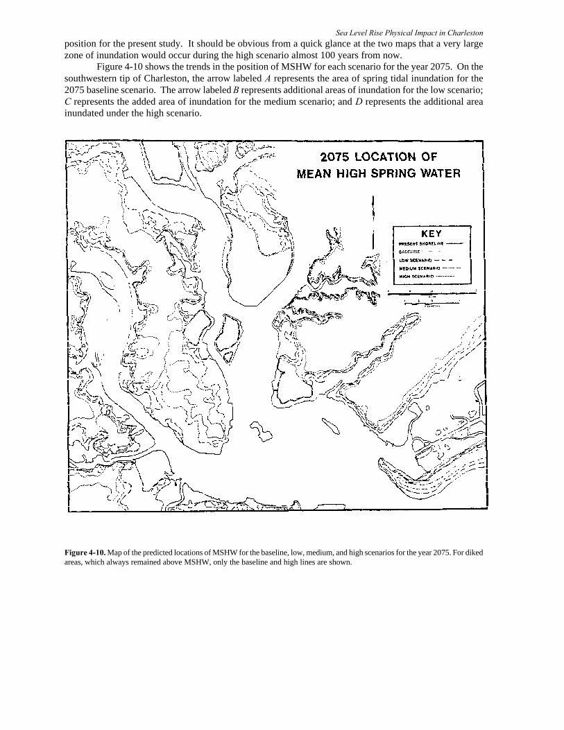
Sea Level Rise Physical Impact in Charlestonposition for the present study. It should be obvious from a quick glance at the two maps that a very largezone of inundation would occur during the high scenario almost 100 years from now.
Figure 4-10 shows the trends in the position of MSHW for each scenario for the year 2075. On thesouthwestern tip of Charleston, the arrow labeled A represents the area of spring tidal inundation for the2075 baseline scenario. The arrow labeled B represents additional areas of inundation for the low scenario;C represents the added area of inundation for the medium scenario; and D represents the additional areainundated under the high scenario.
Figure 4-10. Map of the predicted locations of MSHW for the baseline, low, medium, and high scenarios for the year 2075. For dikedareas, which always remained above MSHW, only the baseline and high lines are shown.
Sea Level Rise Physical Impact in Charleston
Baseline Map-Year 2025
The baseline map for 2025 (see Figure 4-9) was generated to represent the future shoreline and storm surgechanges under current rates of sea level rise, which effected an 11 cm (0.4 ft) rise by 2025. When comparedwith existing (1980) conditions shown in Figure 4-8, there are few significant changes. An average of 30m (100 ft) of inundation occurred along the western shore of the Ashley River, but the new MSHW was stillwithin the astronomic tidal elevations and thus within high marsh vegetation. Along vertical seawalls andspoil dikes, the MSHW was already considered to be at the base of the structure; thus, there were nodetectable changes along the man-made shorelines. The accretionary trends along the islandbeachesdominated over the small amount of inundation. The extensive marsh between Mount Pleasant andSullivans Island was already mostly below MSHW, except for spoil islands along the Intracoastal Waterwayand areas fringing the highland. In fact, considering the accuracy of the computer-plotted contours and the± 15 m (50 ft) precision in measuring the changes between contours, there was essentially no changebetween present (1980) and the baseline for 2025 along interior shorelines. However, along shorelineswhich can be historically documented to be undergoing long-term deposition or erosion, the use of abaseline composed of a historical trend component is important. Inundation as a separate factor is notnecessary because it is inherently included in the historical trend analysis.
The changes in shoreline and storm surge positions for the scenarios in 2025 were small and difficultto display at page-size scales. The shape of the study area is also difficult to illustratein sections and still retain any sense of area-wide comparisons. Thus, the results for the 2025 high scenarioonly are shown in Figure 4-9. The low and medium scenario results are not shown but can be visuallyplaced between the high and baseline positions. The results are described below; the reader should referto Figure 4-9 during the following discussion.
2025 Low Scenario
This scenario represented a total rise in sea level of 28 cm (0.9 ft) but only 17 cm (0.5 ft) above thebaseline for 2025. The changes in the MSHW would be very small compared to the baseline. Inundationat the marsh stations ranged between 0 and 75 m (0-250 ft). As expected, changes in areas of narrowmarshes that fringe developed highland, such as along James Island, would not be discernible because ofgreater slopes (and the limitations of computer interpolation). Mount Pleasant, formed on an old barrierisland itself, rises sharply above the marsh fill behind Sullivans island; there would be little or no changein MSHW on all sides. Parts of Sullivans Island would become erosional, while the bulge in the lee of thejetties would slow its growth.
The changes in the 10- and 100-year storm surges would be small, generally less than 60 m (200 ft).A 28 cm (0.9 ft) rise obviously was not large enough to exceed any breaks in slope. The most significantchange would occur on Sullivans Island, all of which is currently within the l00-year flood zone. The 10-yearflood zone was predicted to dissect the island across contiguous low areas.
2025 Medium Scenario
The medium 2025 scenario of a 46 cm (1.5 ft) rise in sea level did not cause many changes in theshoreline position of consequence to developed property. At a total elevation of 1.4 m (4.6 ft) above presentMSL, the new MSHW position was close to but below the 1.5 m (5 ft) contour, which is the practical lowerlimit for construction of permanent structures. Thus, while there would be no cases of complete structuralproperty damage along the harbor shoreline, many structures would be placed in the zone of yearlyastronomical flooding. This pattern was typical for the entire western shore of the Ashley River, which wasprimarily low density residential property.
Few structures would be included in the 10-year flood zone in this scenario, which ranged between1.8 and 2.3 m (6.0-7.5 ft) above present MSL. Some new areas of residential property would be located inthe 100-year flood zone, particularly between the Ashley River and Wappoo Creek (near station 11 onFigure 4-1).
The shoreline in the city of Charleston has areas that would lose up to 75 m (250 ft) due to
Sea Level Rise Physical Impact in Charleston
erosion/inundation, particularly in the middle part of the peninsula. Although industrially developed, this
middle section has not been landfilled to the extent which occurred to the north (U.S. Navy facilities) andsouth (port facilities and residential). Therefore, a narrow neck of land with smaller areas above the 10- and100-year storm surges occurred. North Charleston, up to 10 m (33 ft) above MSL, would show even fewershoreline changes, except along the cutbank of the Ashley River. Most of the Cooper River shoreline iscomposed of bulkheads and docks for the U.S. Navy Reservation and would not be affected. This area alsowould show regular inland shifts in the 10- and 100-year flood zones of about 75m (250 ft). The historicaldistrict on the Charleston peninsula had no changes along the man-made shorelines. The seawalls range inelevation between 1.5 and 2.7 m (5-9 ft) above present MSL. Thus, increasing periodicity of flooding
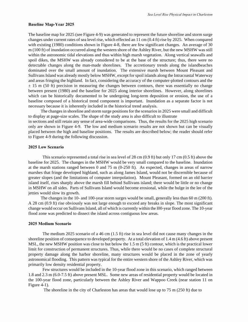
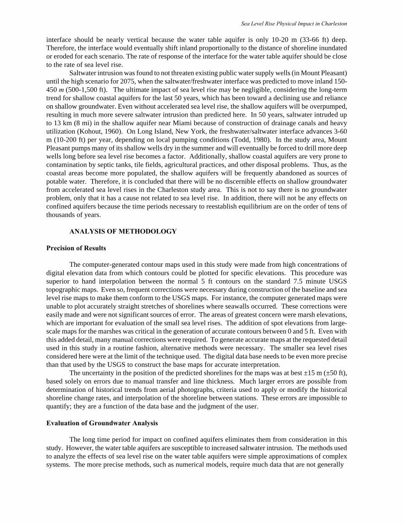
Figure 4-11. Map of the predicted locations of the 100-year storm surge for the baseline, low, medium, and high scenarios forthe year 2075. For diked areas, which always remained above the 100-year surge, only the baseline and high lines were shown.Some of the diked spoil areas were affected under the medium and high scenarios.
Sea Level Rise Physical Impact in Charleston
was of more concern than inundation for this scenario. Of great importance is the projection that some ofthe key arteries of the city would be regularly flooded. The 10-year flood zone moved inland about 75 m(250 ft) in densely populated areas on the west side. The 100-year flood zone became scattered islands ofhigh ground down the center of the peninsula.
Sullivans Island was the area of most serious impact. The causeway connecting the island to themainland would be barely above spring tidal elevations. Any storm or unusual astronomical tides wouldregularly cut off access to and from the island. The projected position of MSHW was landward of the firstrow of houses in the middle section of the island. Erosion of this section would supply sediment to thewestern end of the island, parts of which were still accreting. Wave refraction caused by the jetties wouldcontinue to cause accretion near station 50 (Figure 4-1). Areas above the 10-year flood would be limitedto a narrow strip of land down the center of the island [the only part higher than 2.3 m (7.5ft) MSL]. Furtheraccretion into the harbor would be limited by the deep channel and strong ebb currents, which would carrysand back out the jetties.
2025 High Scenario
There would be few additional changes in the shoreline inundation/erosion trends for this scenario,with some notable exceptions. Large movement in the MSHW position occurred on both sides of WappooCreek, west of the Ashley River. The scenario elevation of MSHW at 1.6 m (5.2 ft) above present MSLbarely exceeded the present 1.5 m (5 ft) contour. The maps showed shoreline positions behind someexisting structures and several islands of highland would be isolated in the southwestern part of the studyarea. Although the 10-year flood zone would get progressively larger, most of the areas above the 100-yearflood west of the Ashley would now be in the flood zone.
On the peninsula, there would still be few serious shoreline problems. The newly filled anddeveloped commercial area north of the Ashley River bridge (station 8, Figure 4-1) would be within the newintertidal zone. Otherwise, existing seawalls were high enough to prevent daily inundation. The 10-yearflood would have moved 90 m (300 ft) inland of the present position. Only small areas would be above the100-year flood along the historic district.
Currently, the town of Mount Pleasant is divided in half by a small water body (Shem Creek), whichseparates two highland areas. As old barrier islands, both sections are relatively high and flat. Shorelineand flood position changes would be generally small and regular, even along the convoluted areas.
Few if any structures in Mount Pleasant would be affected by shoreline movement for this scenario.The largest changes would be along the mainland facing Sullivans Island (Figure 4-9); MSHW shifted upto 225 m (750 ft) inland of its baseline position.
The causeway to Sullivans Island would be regularly flooded during spring tides, that is, every 14days. Sullivans Island itself would have continued to narrow from both shorelines. There would no longerbe any accretion on the southern end and the western tip was barely maintained by a seawall. A second rowof houses would be threatened by erosion and storm waves. The 10-year flood lines would have changedlittle; there would still be a narrow corridor barely above the 2.5m (8.1 ft) elevation.
Even at the highest rise for 2025, there would be no effects on the diked spoil areas throughout theharbor. Dike elevations range between 4.3 and 7,3 m (14-24 ft) above present MSL and thus would protectthe spoil areas from even the 100-year storm surge.
Baseline Map-Year 2075
Projections of historical trends in shoreline position and sea level rise were used to create the 2075baseline maps (Figure 4-10). The sea level rise of 24 cm (0.8 ft) was practically the same as the 2025 lowscenario, which had a 28 cm (0.9 ft) rise. There were few areas of significant change. The new MSHW,at 1.2 m (3.9 ft), would still be below normal astronomical tides, and there would have been a graduallandward shift in marsh vegetation of a few tens of meters at the most. The only structural loss along theshoreline would have occurred in scattered locations along the seaward row of homes on Sullivans Island.Expansion of the 10- and 100-yea r flood zones would be highly variable but would average some 60m (200ft).
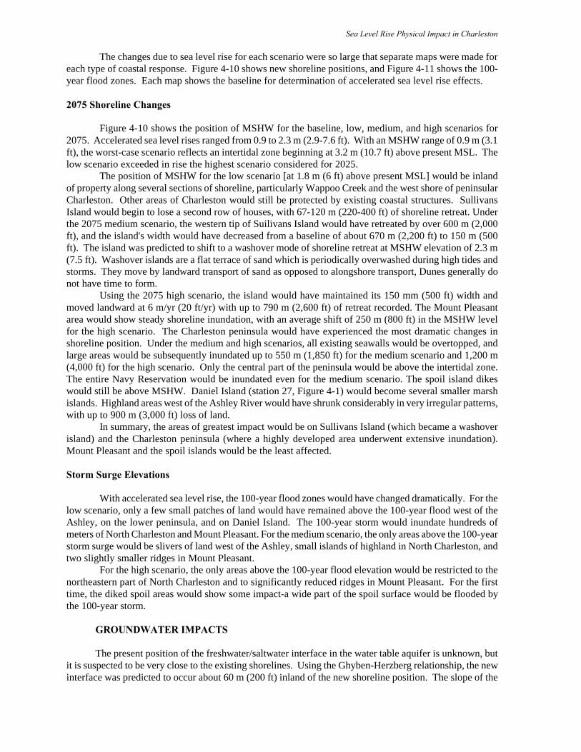
Sea Level Rise Physical Impact in Charleston The changes due to sea level rise for each scenario were so large that separate maps were made for
each type of coastal response. Figure 4-10 shows new shoreline positions, and Figure 4-11 shows the 100-year flood zones. Each map shows the baseline for determination of accelerated sea level rise effects.
2075 Shoreline Changes
Figure 4-10 shows the position of MSHW for the baseline, low, medium, and high scenarios for2075. Accelerated sea level rises ranged from 0.9 to 2.3 m (2.9-7.6 ft). With an MSHW range of 0.9 m (3.1ft), the worst-case scenario reflects an intertidal zone beginning at 3.2 m (10.7 ft) above present MSL. Thelow scenario exceeded in rise the highest scenario considered for 2025.
The position of MSHW for the low scenario [at 1.8 m (6 ft) above present MSL] would be inlandof property along several sections of shoreline, particularly Wappoo Creek and the west shore of peninsularCharleston. Other areas of Charleston would still be protected by existing coastal structures. SullivansIsland would begin to lose a second row of houses, with 67-120 m (220-400 ft) of shoreline retreat. Underthe 2075 medium scenario, the western tip of Suilivans Island would have retreated by over 600 m (2,000ft), and the island's width would have decreased from a baseline of about 670 m (2,200 ft) to 150 m (500ft). The island was predicted to shift to a washover mode of shoreline retreat at MSHW elevation of 2.3 m(7.5 ft). Washover islands are a flat terrace of sand which is periodically overwashed during high tides andstorms. They move by landward transport of sand as opposed to alongshore transport, Dunes generally donot have time to form.
Using the 2075 high scenario, the island would have maintained its 150 mm (500 ft) width andmoved landward at 6 m/yr (20 ft/yr) with up to 790 m (2,600 ft) of retreat recorded. The Mount Pleasantarea would show steady shoreline inundation, with an average shift of 250 m (800 ft) in the MSHW levelfor the high scenario. The Charleston peninsula would have experienced the most dramatic changes inshoreline position. Under the medium and high scenarios, all existing seawalls would be overtopped, andlarge areas would be subsequently inundated up to 550 m (1,850 ft) for the medium scenario and 1,200 m(4,000 ft) for the high scenario. Only the central part of the peninsula would be above the intertidal zone.The entire Navy Reservation would be inundated even for the medium scenario. The spoil island dikeswould still be above MSHW. Daniel Island (station 27, Figure 4-1) would become several smaller marshislands. Highland areas west of the Ashley River would have shrunk considerably in very irregular patterns,with up to 900 m (3,000 ft) loss of land.
In summary, the areas of greatest impact would be on Sullivans Island (which became a washoverisland) and the Charleston peninsula (where a highly developed area underwent extensive inundation).Mount Pleasant and the spoil islands would be the least affected.
Storm Surge Elevations
With accelerated sea level rise, the 100-year flood zones would have changed dramatically. For thelow scenario, only a few small patches of land would have remained above the 100-year flood west of theAshley, on the lower peninsula, and on Daniel Island. The 100-year storm would inundate hundreds ofmeters of North Charleston and Mount Pleasant. For the medium scenario, the only areas above the 100-yearstorm surge would be slivers of land west of the Ashley, small islands of highland in North Charleston, andtwo slightly smaller ridges in Mount Pleasant.
For the high scenario, the only areas above the 100-year flood elevation would be restricted to thenortheastern part of North Charleston and to significantly reduced ridges in Mount Pleasant. For the firsttime, the diked spoil areas would show some impact-a wide part of the spoil surface would be flooded bythe 100-year storm.
GROUNDWATER IMPACTS
The present position of the freshwater/saltwater interface in the water table aquifer is unknown, butit is suspected to be very close to the existing shorelines. Using the Ghyben-Herzberg relationship, the newinterface was predicted to occur about 60 m (200 ft) inland of the new shoreline position. The slope of the
Sea Level Rise Physical Impact in Charleston
interface should be nearly vertical because the water table aquifer is only 10-20 m (33-66 ft) deep.Therefore, the interface would eventually shift inland proportionally to the distance of shoreline inundatedor eroded for each scenario. The rate of response of the interface for the water table aquifer should be closeto the rate of sea level rise.
Saltwater intrusion was found to not threaten existing public water supply wells (in Mount Pleasant)until the high scenario for 2075, when the saltwater/freshwater interface was predicted to move inland 150-450 m (500-1,500 ft). The ultimate impact of sea level rise may be negligible, considering the long-termtrend for shallow coastal aquifers for the last 50 years, which has been toward a declining use and relianceon shallow groundwater. Even without accelerated sea level rise, the shallow aquifers will be overpumped,resulting in much more severe saltwater intrusion than predicted here. In 50 years, saltwater intruded upto 13 km (8 mi) in the shallow aquifer near Miami because of construction of drainage canals and heavyutilization (Kohout, 1960). On Long Island, New York, the freshwater/saltwater interface advances 3-60m (10-200 ft) per year, depending on local pumping conditions (Todd, 1980). In the study area, MountPleasant pumps many of its shallow wells dry in the summer and will eventually be forced to drill more deepwells long before sea level rise becomes a factor. Additionally, shallow coastal aquifers are very prone tocontamination by septic tanks, tile fields, agricultural practices, and other disposal problems. Thus, as thecoastal areas become more populated, the shallow aquifers will be frequently abandoned as sources ofpotable water. Therefore, it is concluded that there will be no discernible effects on shallow groundwaterfrom accelerated sea level rises in the Charleston study area. This is not to say there is no groundwaterproblem, only that it has a cause not related to sea level rise. In addition, there will not be any effects onconfined aquifers because the time periods necessary to reestablish equilibrium are on the order of tens ofthousands of years.
ANALYSIS OF METHODOLOGY
Precision of Results
The computer-generated contour maps used in this study were made from high concentrations ofdigital elevation data from which contours could be plotted for specific elevations. This procedure wassuperior to hand interpolation between the normal 5 ft contours on the standard 7.5 minute USGStopographic maps. Even so, frequent corrections were necessary during construction of the baseline and sealevel rise maps to make them conform to the USGS maps. For instance, the computer generated maps wereunable to plot accurately straight stretches of shorelines where seawalls occurred. These corrections wereeasily made and were not significant sources of error. The areas of greatest concern were marsh elevations,which are important for evaluation of the small sea level rises. The addition of spot elevations from large-scale maps for the marshes was critical in the generation of accurate contours between 0 and 5 ft. Even withthis added detail, many manual corrections were required. To generate accurate maps at the requested detailused in this study in a routine fashion, alternative methods were necessary. The smaller sea level risesconsidered here were at the limit of the technique used. The digital data base needs to be even more precisethan that used by the USGS to construct the base maps for accurate interpretation.
The uncertainty in the position of the predicted shorelines for the maps was at best ±15 m (±50 ft),based solely on errors due to manual transfer and line thickness. Much larger errors are possible fromdetermination of historical trends from aerial photographs, criteria used to apply or modify the historicalshoreline change rates, and interpolation of the shoreline between stations. These errors are impossible toquantify; they are a function of the data base and the judgment of the user.
Evaluation of Groundwater Analysis
The long time period for impact on confined aquifers eliminates them from consideration in thisstudy. However, the water table aquifers are susceptible to increased saltwater intrusion. The methods usedto analyze the effects of sea level rise on the water table aquifers were simple approximations of complexsystems. The more precise methods, such as numerical models, require much data that are not generally
Sea Level Rise Physical Impact in Charleston
available or accurately known. Even the USGS models to simulate the movement of the freshwater/saltwaterinterface during Pleistocene sea level fluctuations in a region with an extensive data base, have beenextremely difficult to calibrate.
The shallow aquifer in the study area was only 10-20 m (33-66 ft) thick; thus, the Ghyben-Herzbergprinciple predicted 60 m (200 ft) of saltwater intrusion beyond the new shoreline position for each scenario.In thicker aquifers, the Ghyben-Herzberg principle works well as a conservative estimate. The mainuncertainties in its application are the degree to which the freshwater system equilibrates with the rise insaltwater head and the net effect of increased discharge. Since little is known about how these two processesaffect the response of the water table, they have not been incorporated into this study. However,groundwater effects from sea level rises up to 200 cm (6.5 ft) appear to be minor compared with otherprocesses that are causing more rapid and extreme saltwater intrusion. Studies should be made to test theimpact of sea level rise on large water table aquifers that are well understood, such as the Long Island glacialaquifer, to determine if groundwater effects are an important consideration to evaluate.
General Applicability
The methods developed in this pilot study used data that are readily available for most coastal regions(i.e., various scales of topographic maps, aerial photographs, flood-hazard boundary maps) and widelyapplicable. The methods used to predict the position of the shoreline for the baseline and scenario mapshave been described in detail in this report. They are based on general principles of coastal geology and canbe applied to almost any shoreline type or location. The general applicability of this method should betested in other areas, especially to test for differences in geomorphology, tide regime, and local effects suchas high subsidence rates. The coastal geomorphology and physical setting of the Chesapeake area, forexample, may require a very different ordering of the dominant processes. The tidal range is smaller, andit borders a major estuary. The sediment flux will be smaller for both fine-grained, suspended sedimentsand littoral sediments eroding from the headlandsin the bay and at the entrance capes.
REFERENCES
Brown, P. J. 1976. "Variations in South Carolina Coastal Morphology." In M. 0. Hayes and T. W. Kana, eds.,Terrigenous Clastic Depositional Environments.Guidebook to field trip sponsored by the AmericanAssociation of Petroleum Geologists, pp. II-2-II-15.
Bruun, P 1962. "Sea-Level Rise as a Cause of Shore Erosion." Journal of the Waterways and Harbors Division 88(WW1):117-130.
Colquhoun, D. J., T. A. Bond, and D. Chappel. 1972. "Santee Submergence: Example of Cyclic Submerged andEmerged Sequences." Geological Society of America Memoir 133, pp. 475-496.
Cooper, H. H., F. A. Kohout, H. R. Henry, and R. E. Glover. 1964. Sea Water in Coastal Aquifers. U.S. GeologicalSurvey Water-Supply Paper 1613-C.
Finley, R. J. 1981. Hydraulics and Dynamics of North Inlet, South Carolina 1974-1975. GITI report no. 10. FortBelvoir, Va.: Coastal Engineering Research Center.
Hands, E. B. 1981. Predicting Adjustments in Shore and Offshore Sand Profiles on the Great Lakes. CERC technicalaid 81-4. Fort Beivoir, Va.: Coastal Engineering Research Center.
Hathaway, J. C., C. W Poag, R C. Valentine, R. E. Miller, D. M. Schultz, F. T. Manheim, F. A. Kahout, M. E. Bothner, and D. A. Sangrey. 1979. "U.S. Geological Survey Core Drilling on the
Atlantic Shelf." Science 206(4418):515-527. Henry, H. R. 1962. Transitory Movements of the Salt- Water Front in an Extensive Artesian Aquifer. U.S. Geological
Survey Professional Paper 450-B, pp. 1387-1388.Herzberg, A. 1961. "Die Wasserversorgung Einiger Nordseebader, Munich,” Journal Gasbeleuchtung und
Wasserversorgung 44:815-819, 842-844.Hicks, S. D. 1978. "An Average Geopotential Sea Level Series for the United States." Journal of Geophysical
Research 83(C3):1377-1379.Hicks, S. D., and J. E. Crosby. 1974. Trend and Variability of Yearly Mean Sea Level, 1893-1972. NOAA technical
memorandum NOS-13. Rockville, Md.: Department of Commerce.
Sea Level Rise Physical Impact in Charleston
Hicks, S. D., H. A. Debaugh, Jr., and L. E. Hickman, Jr. 1983. Sea Level Variations for the United States, 1855- 1980. NOAA report. Rockville, Md.
Jelesnianski, C. P. 1972. SPLASH (Special Program to List Amplitudes of Surges from Hurricanes) 1. LandfallStorms. Silver Spring, Md.: NOAA technical memorandum NWS TDI,46.
Jelesnianski, C. P., and J. Chen. 1984 (in press). SLOSH (Sea, Lake, and Overland Surges from Hurricanes). NOAAtechnical memorandum. Silver Spring, Md.: NOAA.
Kana, T 1977. "Suspended Sediment Transport at Price Inlet, S.C." In Proceedings of Coastal Sediments '77. New York: American Society of Civil Engineers, pp. 366-382.
Kohout, F. A. 1960. "Cyclic Flow of Salt Water in the Biscayne Aquifer of South-Eastern Florida." Journal of Geophysical Research 65 (7): 2133-2141.
Kraft, J. C. 1971. "Sedimentary Facies Patterns and Geologic History of a Holocene Marine Transgressions Bulletinof the Geological Society America 82:2131-2158.
Landers, H. 1970. "Climate of South Carolina." In Climates of the States: South Carolina, Climatography of theUnited States. Asheville, N.C.: 6038, ESSA,Environmental Data Service.
Leatherman, S. P. 1977. "Overwash Hydraulics and Sediment transport." In Proceedings of Coastal Sediments '77. New York: American Society of Civil Engineers, pp. 135-148.
Mercer, J. W., S. P. Larson, and C. R. Faust. 1980. "Simulation of Saltwater interface Motion." Ground Water 18(4):374-385.
Michel, J., T W. Kana, and M. 0. Hayes. 1982. Hypothetical Shoreline Changes Associated with Various Sea-LevelScenarios for the United States: Case Study, Charleston, South Carolina. Report to ICF under contract toEPA. Columbia, S.C.: RPI.
Myers, V. 1975. Storm-Tide Frequencies on the South Carolina Coast. Silver Spring, Md.: National WeatherService, Office of Hydrology.
Nummedal, D., G. F. Oertel, D. K. Hubbard, and A. C. Hine. 1977. "Tidal Inlet Variability: Cape Hatteras to CapeCanaveral." In Proceedings of Coastal Sediments '77. New York: American Society of Civil Engineers, pp.543-562.
Parker, G. G. 1955. "Salt-Water Contamination of the Aquifer from tidal Canals." In Water Resources of SoutheasternFlorida. U.S. Geological Survey Water Supply Paper 1255, pp. 682-707.
Pinder, G. F., and H. H. Cooper, Jr. 1970. "A Numerical Technique for Calculating the Transient Position of the Saltwater Front." Water Resources Research 6(3):875-882.
Research Planning Institute. Unpublished nearshore survey data for Isle of Palms, Kiawah Island, and SeabrookIsland, 1974-83. Columbia, S.C.: RPI.
South Carolina Water Resources Commission. 1979. Cooper River Controlled Low-Flow Study. Columbia, S.C.: Report no. 131.
Stephen, M. F., P. J. Brown, D. M. FitzGerald, D. K. Hubbard, and M. 0. Hayes. 1975. Beach Erosion Inventory ofCharleston County, S.C.: A Preliminary Report. Columbia, S.C.: University of South Carolina, SouthCarolina Sea Grant technical report no. 4.
Stringfield, F. 1 1966. Artesian Water in Tertiary Limestone in the Southeastern States. Washington, D.C.: U.S.Geological Survey Professional Paper 517.
Todd, D. K. 1980. Groundwater Hydrology. New York: John Wiley & Sons. U.S. Army Corps of Engineers. 1966. Survey Report on Cooper River, S.C. (Shoaling in Charleston Harbor). U.S.
Army Corps of Engineers, Charleston, S.C., District.U.S. Army Coastal Engineering Research Center. 1977. Shore Protection Manual. 3 vols. Washington, D.C.:
Superintendent of Documents.U.S. Department of Commerce. 1979. State of South Carolina Coastal Zone Management Program and Final
Environmental Impact Statement. Rockville, Md.: NOAA.U.S. Department of Commerce. 1981. 77de 7hbles, North America. Rockville, Md.: NOAA.Ward, L. G., and D. D. Domeracki. 1979. "Hydrodynamic and Sedimentologic Processes in Tidal Channels." In
Proceedings with Abstracts, International Meeting Holocene Marine Sediments. North Sea Basin, Texel, Holland.
Wilson, W. E. 1982. Estimated Effects of Projected Ground-Water Withdrawals on Movement of the Saltwater Frontin the Floridan Aquifer, 1976-2000. West-Central Florida. U.S. Geological Survey Water-Supply Paper 2189.
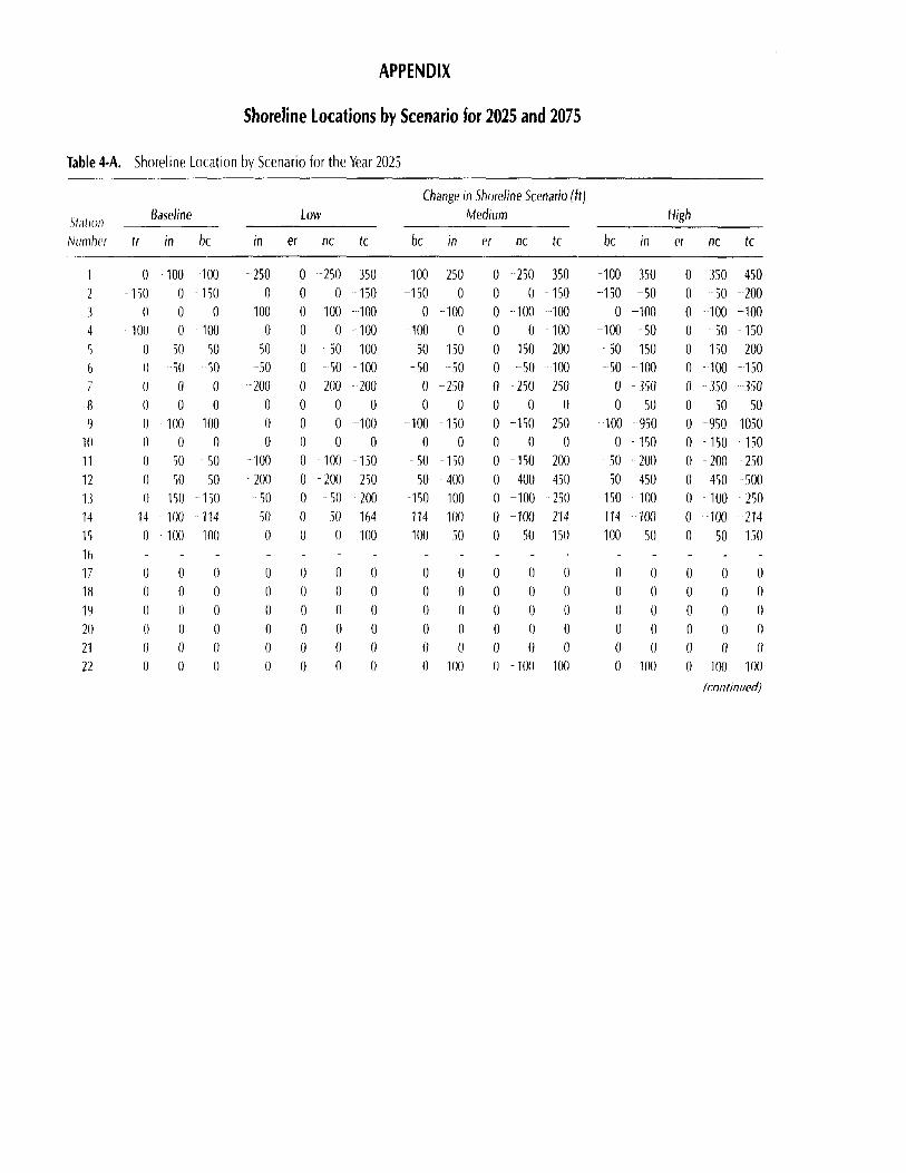
Sea Level Rise Physical Impact in Charleston
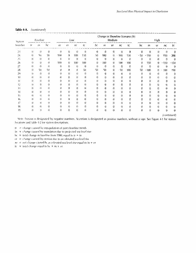
Sea Level Rise Physical Impact in Charleston
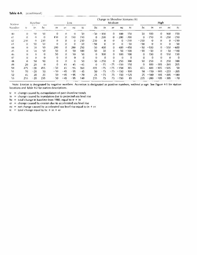
Sea Level Rise Physical Impact in Charleston
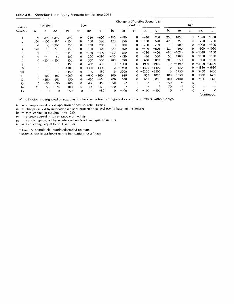
Sea Level Rise Physical Impact in Charleston
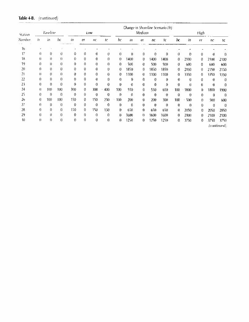
Sea Level Rise Physical Impact in Charleston
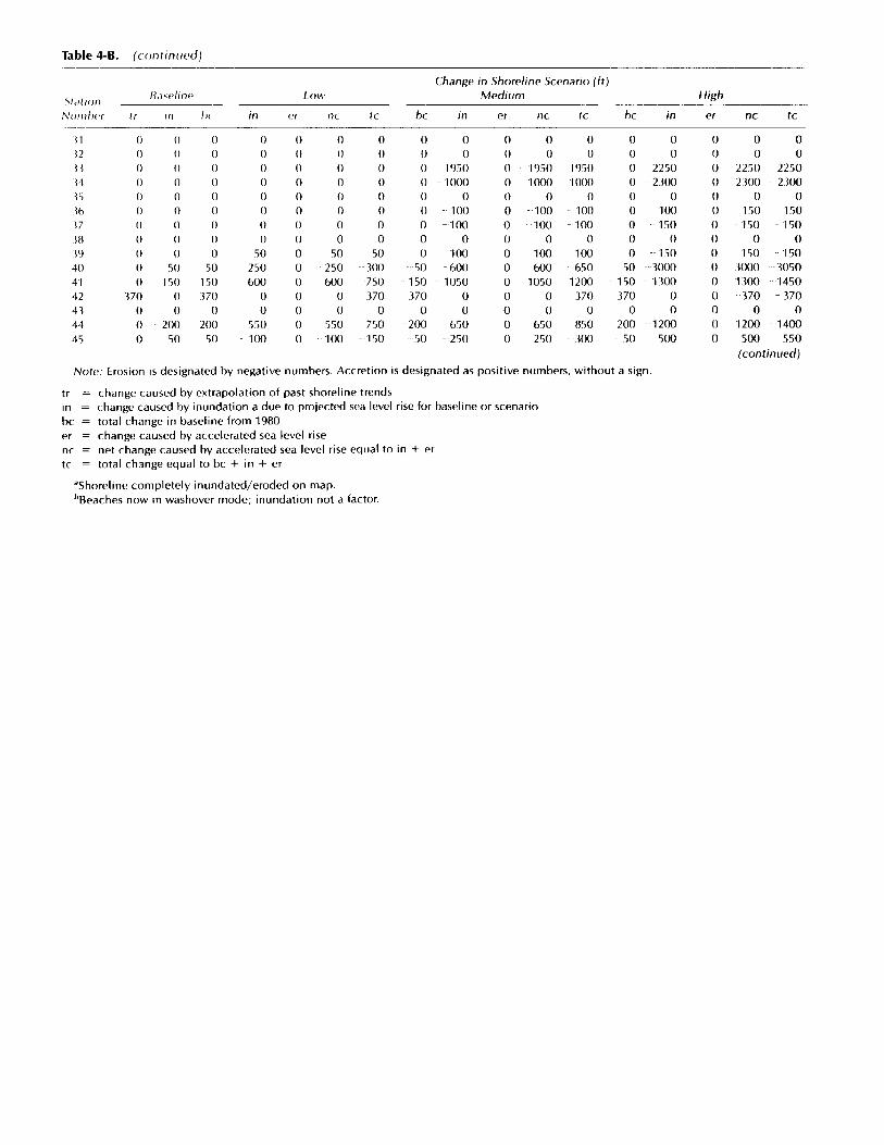
Sea Level Rise Physical Impact in Charleston
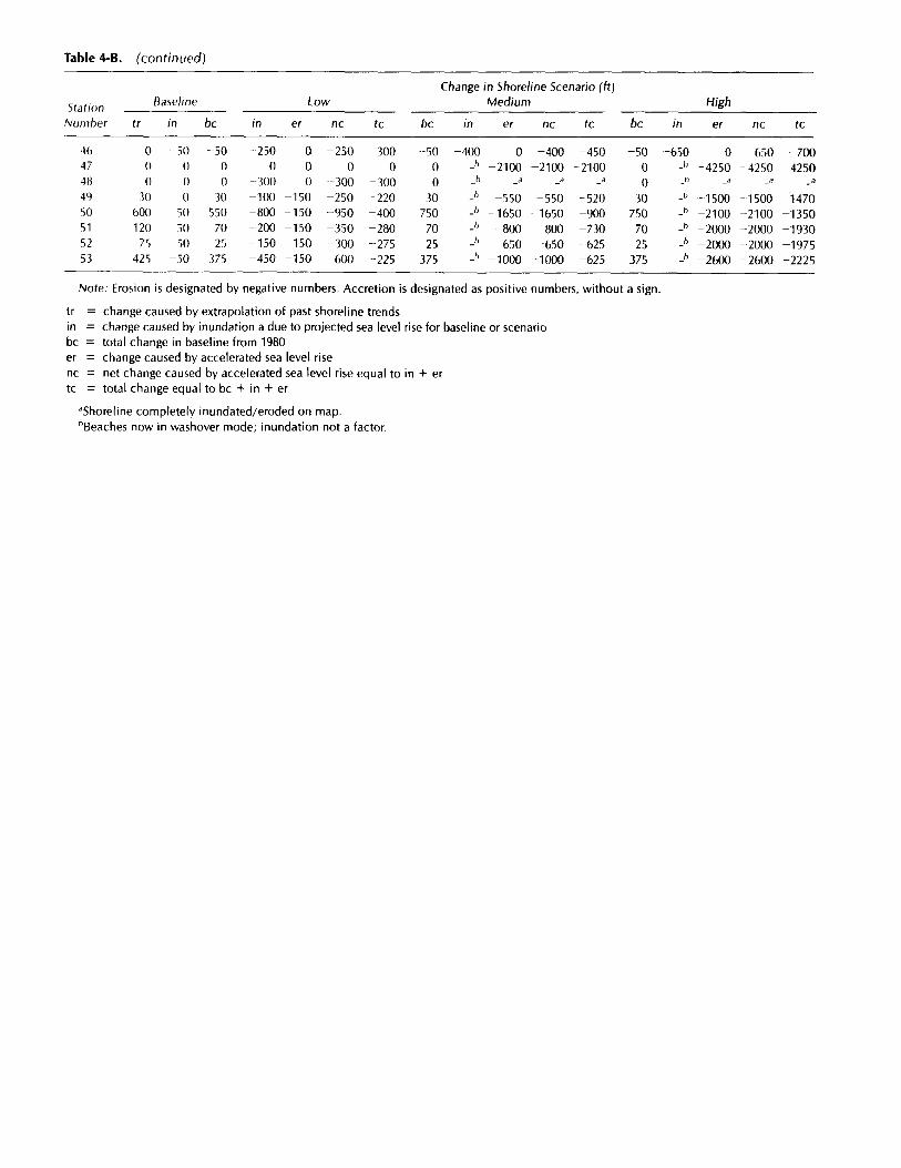
Sea Level Rise Physical Impact in Charleston