the poincar© conjecture - icm 2006

The Poincaré Conjecture

John W. Morgan

1. Introduction

It is a great pleasure for me to report on the recent spectacular developments concern-ing the Poincaré Conjecture.

Grigory Perelman has solved the Poincaré Conjecture. He has shown that, asPoincaré conjectured, any closed, simply connected 3-manifold is homeomorphic tothe 3-sphere.

The paper in which Poincaré posed this problem in 1904 ([14]) marked, in myview, the founding of topology as an independent discipline within pure mathematics.Over the intervening 100 years, the problem has been much studied and generalized,and many related problems have been solved. It has been linked, in one way oranother, with most of the progress in topology in the last 100 years. While relatedproblems have been solved, the original conjecture stood untouched, resisting all at-tempts. Before Perelman’s work, there had been no progress on toward solving thePoincaré Conjecture, and many viewed it as the siren song of Topology, for many aboat had foundered on the rocks trying to reach it. There have been innumerable pro-posed proofs and proposed counter-examples, but none, before Perelman’s, withstoodscrutiny.

Solving the Poincaré Conjecture is a signal achievement for Perelman, but it isalso a signal achievement for all of mathematics, for it gives a measure of how farour understanding of the subject has advanced in the last 100 years. To paraphraseNewton, Perelman has seen far, but to do so he stood on the shoulders of giants whocame before him. One giant, in particular, stands out. He is Richard Hamilton. Overa period of 25 years, Hamilton painstakingly built the solid and elaborate foundationupon which Perelman constructed the edifice of his proof. Without Hamilton’s work,Perelman’s would not have been possible.

One of the most interesting aspects of the resolution of the Poincaré Conjecture isthe nature of the solution. While the problem is purely topological in its formulation,the proof is not. The proof uses deep techniques and results from other areas ofmathematics, namely analysis and differential geometry. It is not at all clear a priorithat these ideas have any relevance to the Poincaré Conjecture, but in the end theyturn out to be the only way (so far) to approach this question successfully.

My goal in this article is to give you a sense of the importance, centrality, andthe depth of the Poincaré Conjecture. Then I will discuss surfaces and 3-dimensionalspaces and describe how topologists think about them. Next, I will formulate and

Proceedings of the International Congressof Mathematicians, Madrid, Spain, 2006© 2007 European Mathematical Society

714 John W. Morgan

explain the statement of the conjecture. Then I will give an overview of the ideas thatgo into the solution – Ricci flow, Ricci flow with surgery, and finite-time extinction forRicci flow with surgery when applied to a simply connected 3-manifold. The latterwill be a very superficial view of the mathematics. I refer the reader to the body ofHamilton’s work [2] as well as to Perelman’s preprints [11], [13], and [12] for moreprecise statements of the analytic and geometric results that are needed.

2. Problems in mathematics

2.1. A brief history. The central role of problems in mathematics goes back tothe Greeks (at least). From them we have the famous examples of the question ofsquaring the circle and of doubling the cube using only compass and straightedge,among others1. Starting in the 16th century mathematicians challenged each otherwith problems and by the 18th century learned societies posed problems to the generalmathematical community often with prizes awarded for their solution. The mostfamous set of problems in modern mathematics is Hilbert’s 23 problems posed atthe International Congress of Mathematicians in Paris in 1900; see [7]. These wereposed for an entirely different reason and were of an entirely different order from mostof the problems heretofore seen in mathematics. Hilbert’s goal was to lay out whathe considered central problems across the entire subject, problems, whose solutionsand even attempted solutions, he thought would be important, indeed central, for thedevelopment of the subject in the century that was about to begin. He introduced hisproblems, making it clear that he saw them being linked to the future development ofthe subject by saying “Who among us would not be glad to lift the veil behind whichthe future lies hidden; to case a glance at the next advances of our science and at thesecrets of its development during the future centuries?” Some of the problems werealready well known before Hilbert’s address, for example the Riemann hypothesis,and others were formulated for the first time by Hilbert. Much progress has beenmade on many, but not all, of these problems. Some still remain open. And asHilbert foresaw, they did play an instrumental role in mathematics. They formedthe backdrop against which a significant portion of the mathematical development ofthe 20th century was measured. To solve one of Hilbert’s problems was to enter theMathematical Hall of Fame.

A new list of seven problems was proposed in 2000 by the Clay MathematicsFoundation, the Clay Millennium Problems. As the Clay Foundation makes clear, thechoice of the timing (100 years after Hilbert’s address) and the location (Paris, the sameas the location of Hilbert’s address) was explicitly made to honor Hilbert’s address andthe role his problems had indeed played in twentieth century mathematics. They arealso hopeful that their list of problems will have a similar impact on mathematics in thetwenty-first century. The problems which they introduced are called the 7 Millennium

1For more details on the role of problems in mathematics, see the article by Jeremy Gray in [5].

The Poincaré Conjecture 715

Problems. Attached to each of the problems is a prize of $1,000,000 for its successfulsolution. There is one problem on this list in common with Hilbert’s list, the Riemannhypothesis. The other six are more recent problems.

One of the Clay Millennium Problems is the Poincaré Conjecture. Aside from theRiemann Hypothesis it is the oldest on the list, dating from 1904. It is the problemwhose solution we are celebrating. It is the first of the Millennium Problems to besolved. None of the others seems ripe for solution. But of course, before its solutionneither did the Poincaré Conjecture.

2.2. The role of problems. What makes a good problem and what role do prob-lems play in mathematics? Quoting again from Hilbert’s address to the InternationalCongress in 1900, “I should still more demand for a mathematical problem if it is tobe perfect; for what is clear and easily comprehended attracts, the complicated repelsus. Moreover, a mathematical problem should be difficult in order to entice us, yetnot completely inaccessible, lest it mock our efforts. It should be to us a signposton the tortuous paths to hidden truths, ultimately rewarding us by the pleasure in thesuccessful solution.”

Hilbert is making several points here. If a problem is sufficiently difficult that itcannot be immediately solved but if it is not so difficult as to be inaccessible, then itwill stimulate much mathematical activity and progress as different approaches aretried. History is replete with examples of extraordinary mathematics being createdin an attempt to solve a long-standing problem. Sometimes these attempts result inpartial solutions or further clarifications of the problem under consideration, othertimes, the mathematics does not reach its intended target, but ends up being usefulin a completely different area. Good problems stimulate mathematical activity bothdirectly related to the problem and in other surrounding areas of mathematics.

Another point that Hilbert is making is that problems become more famous asthey resist more and more different attempts at solution, and that, when they reachthis status, they are used a measuring stick against which the power of new ideasis tested. If a new idea makes progress on an old and famous problem, then it hasdemonstrated its originality, depth and power. Of course, solving such long-standingproblems bestows honor in the first instance on the solver because he or she hassucceeded where all others failed, but also most of the time it is a marker for theprogress of the discipline as a whole. Mathematics has matured to the point whererarely, if ever, is the solution of a significant problem the result entirely of the workof a single mathematician. Rather such advances rest on the general advancement ofunderstanding of the subject and the various previously developed techniques availableto attack the given problem. In the case of the Poincaré Conjecture I have alreadyreferred to the indispensable work of Hamilton on Ricci flow, but Perelman’s argumentalso rests on the modern theory of Riemannian manifolds and the modern theory ofvarious compactness results for spaces of Riemannian manifolds and more generalsingular objects. This theory has been developed over the last 50 to 60 years byan entire army of mathematicians. Hamilton’s work in turn relies on the progress

716 John W. Morgan

in partial differential equations on manifolds, especially parabolic equations such asthe heat equation and the mean curvature flow equation. Again the workers whodeveloped these techniques are too numerous to list.

To me, the most amazing thing about mathematics is that there are mathematicalproblems that are hard enough that their solution requires decades if not centuries ofwork, and yet it is possible by dint of long hard work, many ideas, and incrementaladvances over time to arrive at a solution. Once the perspective is correct and thetechnical power is sufficiently developed, they succumb. They are hard not becausethey are computationally difficult, but because they are conceptually difficult; yet theyare not conceptually too difficult that human beings are incapable of solving them.It just takes us a while to get the perspective correct, to get the right position andwith the right frame of mind to solve them. That the human race is capable of suchadvances is cause for celebration by all of us.

3. The Poincaré Conjecture

This brings us to the problem whose solution we are discussing – the Poincaré Con-jecture. This problem was originally formulated in 1904 by Henri Poincaré [14] nearthe end of a long article on 3-dimensional topology. This article laid out many of thebasic tenets of topology and marked its beginning as an independent field of mathe-matical study. At the end of the article, Poincaré states that there remains one centralquestion to be addressed, “Is every simply connected 3-manifold topologically equiv-alent to the 3-sphere?” In an interesting twist of history, this is not Poincaré’s firstformulation of such a question. Several years earlier he had asked a similar questionwhere the hypothesis of simply connected is replaced by a related (but we now know)weaker condition. After posing this question, Poincaré realized that he knew howto construct counter-examples to that question and that the way to show that theywere indeed counter-examples was to use a topological invariant that he had inventedabout 10 years before; we call it the fundamental group2, and in French it is calledthe ‘groupe de Poincaré.’ Anyway, using this invariant he showed the answer to hisfirst question was ‘no’ and then he formulated the question that lasted 100 years.

The Poincaré Conjecture has all the attributes of an excellent problem. It was sim-ple (for the mathematician) to state. It was a generalization of a well-known propertyof surfaces, so it was a natural guess as to a fundamental fact about 3-dimensionalmanifolds. While simple to state and while being an obvious generalization of aknown mathematical result, it was not easy to resolve, or indeed to make any progressat all on this problem. The problem is a problem purely in topology: the hypothesesare topological and the conclusion is topological. It was attacked by direct topologicalmeans for 100 years without any progress; see [18]. Nevertheless, all this effort wasnot futile. We learned much, just not about this question.

2For a formal definition of this group and all other technical terms see the appendix.


3.1. Mathematics generated by the Poincaré Conjecture. The Poincaré Conjec-ture is an attempt to characterize topologically the simplest of all 3-dimensional man-ifolds, the 3-sphere. In approaching this question, many techniques were developedto study 3-dimensional manifolds. Some of the most important go back to Papakyria-kopoulos [10] in the 1950s. Among these are Dehn’s lemma and the loop theorem andthe sphere theorem. These are incredibly powerful tools for studying 3-manifolds.For example, they allow one to prove the analogue of the Poincaré Conjecture forknots in the 3-sphere. More precisely, Parakyriakipoulos showed that a knot in the3-sphere is topologically equivalent to the unknotted circle if and only if the funda-mental group of the space obtained by removing the knot from the 3-sphere is thesame as the fundamental group of the space obtained by removing the trivial unknottedcircle from the 3-sphere. Using these techniques Waldhausen [20], in the 1960s, gavea complete characterization of a large class of 3-manifolds, but unfortunately fromthe perspective of the Poincaré Conjecture, the class that Waldhausen characterizedis at the other end of the spectrum from simply connected 3-manifolds. Here, we seeattempts to solve the Poincaré Conjecture leading to enormous progress in a closelyrelated area – the study of other 3-manifolds – but saying nothing about the originalconjecture. But this is just the beginning of the story.

In 1960 Smale [17], in one of the most revolutionary advances in topology, real-ized that it was not the case that manifolds were harder and harder to study as theirdimension increased. Before Smale the thinking was: surfaces are understood; wecannot prove central results about 3-dimensional manifolds, so those of higher dimen-sion must be even harder, too hard to even begin to think about until we understand3-dimensional manifolds. Smale generalized the Poincaré Conjecture to all dimen-sions (this was fairly obvious) and then proceeded to solve it in the affirmative in alldimensions 5 and higher. This was the revolution. Four years earlier Milnor [8] hadshown that a closely related question was false starting in dimension 7. In particular,Milnor showed that the smooth version3 of the Poincaré Conjecture was not true inhigher dimensions. Smale and Milnor each won Fields Medals for the works wehave just cited. But this was just the beginning of a 20 year period of unparalleledadvances in topology. Using the ideas of Smale and Milnor and others such as RenéThom, topologists succeeded in answering almost every question that could possiblybe answered about manifolds of dimension 5 and greater. This whole area of topologyis known as ‘surgery theory,’ or ‘Browder–Novikov surgery theory’ after its two maindevelopers; see [1]. The reason that high dimensional manifolds are easier to studythan the ones of dimensions 3 and 4 is that in them there is enough room to movesubmanifolds (e.g., loops and surfaces) around and put them in good position withrespect to each other, whereas in lower dimensional manifolds this is not possible.

By the late 1970s high dimensional manifolds were well understood, and the at-tention of topologists reverted back to their ‘problem children’– dimensions 3 and 4 –and in particular to the Poincaré Conjecture. It was not clear how to proceed. Flushed

3See the appendix.

718 John W. Morgan

with the success in high dimensions (and dare we say the hubris it engendered), manytopologists, myself included, felt that it was just a matter of time before the ‘so-called’low dimensions would succumb to our purely topological techniques. Others, in par-ticular Shing-TungYau, argued strongly that one needed geometric and analytic tools,for example minimal surfaces and special metrics, to attack these low dimensions.From a different direction, Atiyah and Singer were saying ‘Physics takes place in thelow dimensions and could well make an impact.’ The history of the low dimensions isstill being written but the verdict is in and is clear: topologists like myself were wrong;Yau was right; and Atiyah and Singer were right. The evolution to using ever moreanalysis, geometry, and physics to attack questions about manifolds of dimensions 3and 4 is the next part of the story of topology and the Poincaré Conjecture.

3.2. Thurston’s generalization. The next advance in 3-dimensional topology datesfrom the late 1970s and early 1980s. Thurston was applying geometric ideas, inparticular hyperbolic geometry4, to 3-dimensional manifolds. His work led himto formulate a general conjecture about all 3-dimensional manifolds, a conjecturethat says that they could be cut apart in a very precise way into pieces that hadhomogeneous 3-dimensional geometries; see [19] and [15], and see also the appendix.The list of all possible 3-dimensional homogeneous geometries was known classically.Examining this list one sees that by far the most interesting case is the hyperbolicgeometry that Thurston had been studying. It is also immediate from studying the listof possibilities that the Poincaré Conjecture is a very special case of Thurston’s moregeneral conjecture. So here we have the first real progress on the Poincaré Conjecture.This progress consists in embedding the Poincaré Conjecture as a special case of avastly more general conjecture about all 3-dimensional manifolds. Thurston’s workalso established many special cases of his general conjecture, but not a case that relateddirectly to the Poincaré Conjecture. One effect of this was that Thurston’s workconvinced most topologists that his conjecture and therefore the Poincaré Conjecturewas most likely true. (Some would have said definitely true.) For his work Thurstonreceived a Fields Medal in 1982.

3.3. Resolution in dimension four. In the early 1980s there were two advances indimension four. M. Freedman [4] managed to push the higher dimensional argumentsdown into dimension four and to prove the four-dimensional version of the PoincaréConjecture, leaving only the original 3-dimensional version of the conjecture open.This argument required crinkling various surfaces inside the four-dimensional mani-fold infinitely badly in order to get them to fit and the argument could not be made towork with smooth surfaces. Freedman’s work not only solved the four-dimensionalPoincaré Conjecture, it applied to all simply connected four-manifolds. (Unlike di-mension three, there are many simply connected four-manifolds.) At almost the sametime, Donaldson [3], using the Yang–Mill’s equations from physics, showed that

4See appendix.


the analogues of Freedman’s results definitely did not hold for smooth manifolds.Freedman and Donaldson each received a Fields Medal in 1986 for their work onfour-dimensional manifolds.

At this point, 1986, the situation is the following: The Generalized Poincaré Con-jecture has been resolved affirmatively in all dimensions except dimension three. Itis understood that in dimensions four and higher there is a difference between study-ing smooth manifolds and topological manifolds, something that was unsuspected byPoincaré and anyway does not occur in dimension three. Manifolds of dimensionfive and higher, and simply connected topological 4-manifolds were well understood.For all the work in topology related to the Poincaré Conjecture a total of five FieldsMedals over a period of 28 years had been awarded. At the end of this unbelievablefertile period the main outstanding problem was exactly the same as it was at the be-ginning – the Poincaré Conjecture in its original formulation. Furthermore, all directtopological attacks on this problem had yielded no results at all – no special caseshad been solved, no reductions of the problem had been made that showed promiseof yielding essential new insights. While there had been incredible advances in un-derstanding manifolds, what had been clear from the 1950s had been confirmed bythese advances: the Poincaré Conjecture was the central problem in topology.

4. Method of solution

There was, however, progress being made in a different area of mathematics thatwould eventually pave the way for a solution of the Poincaré Conjecture. In 1982Richard Hamilton had developed enough of the theory of the Ricci flow to provethat a compact 3-manifold admitting a Riemannian metric5 of non-negative Riccicurvature in fact admits a Riemannian metric of constant positive sectional curvature;see [6]. In particular, if such a manifold is simply connected, then a classical theorem,essentially going back to Riemann, implies that the Riemannian manifold is isometricto the 3-spheres. In particular, the manifold is diffeomorphic to the S3. While thismight seem significant progress on toward the Poincaré Conjecture, the fact that thehypothesis of Hamilton’s theorem is geometric (non-negative Ricci curvature) and thefact that there was no known way to construct such metrics, meant that while this wasa beautiful theorem in geometric analysis it was not apparent that it represented realprogress on the Poincaré Conjecture. It suggests that it might be possible to attack thePoincaré Conjecture in this way, but whether this method is fruitful for such an attackhad to await further developments. For a general survey of Ricci flow, including mostof Hamilton’s papers, see [2].

There was, however, an interesting relationship, which according to Hamilton wasfirst pointed out to him byYau, between Thurston’s more general conjecture and Ricci

5We discuss Riemannian metrics and curvature in more detail in Section 6 and Ricci flow in more detail inSection 7.

720 John W. Morgan

flow. This relationship operates at two levels. To a first approximation, Thurston’sconjecture posits that a 3-manifold admits a nice metric. Thus, in this more generalconjecture the hypotheses remain topological but the conclusion is geometric. Ifwe are searching for such a nice metric, then we can hope to find it by geometricor analytic techniques. Based on the analogy with the heat flow, one expects Ricciflow to produce such nice metrics. Indeed, in Hamilton’s result, cited above, thisis exactly what happens. This is the reasoning that led Hamilton to hope to applyhis evolution equation for a Riemannian metric, the Ricci flow equation, to the moregeneral problem of constructing homogeneous metrics on 3-manifolds, that is to sayto attack Thurston’s more general conjecture by using Ricci flow. But this reasoningcan be pushed further to operate at a deeper level, Thurston’s conjecture requires acutting or a surgery of 3-manifolds before finding pieces admitting nice metrics. Onthe other hand, the Ricci flow equation, like most non-linear parabolic equations,develops finite-time singularities that must be dealt with. It seems conceivable thatthese issues are of a similar nature. Maybe cutting away the finite-time singularities inorder to continue the Ricci flow would exactly lead to the cutting process required inThurston’s conjecture. This then was the idea: use the Ricci flow on all 3-manifoldsand the singularity development will exactly mimic the cutting process required byThurston’s conjecture.

To study the Ricci flow and to prove results that are relevant to 3-dimensional topol-ogy requires a detailed and delicate analytic and geometric analysis of the Ricci flowequation and the properties of its solutions. So approaching the Poincaré Conjectureand the more general geometrization conjecture of Thurston’s in this way changesthe mathematical techniques and results required to solve the topological problemfrom topological ones (which had been attempted without success) to geometric andanalytical ones, which are more refined and hence hold out the possibility of beingmore powerful, but of course use many deep analytic results and delicate analytictechniques.

Hamilton established some beautiful results about singularity development inRicci flow on 3-manifolds which were suggestive that the entire program might bemade to work, but he could not get good enough control on the singularities that de-velop in finite time to prove that he could always do surgery and continue the process.Here is where Perelman enters the story. He realized that in addition to the propertiesthat Hamilton had established there was one more crucial one that Hamilton had notconsidered, a volume non-collapsing result. Perelman introduced a beautiful newconcept, unlike anything in Hamilton’s work, that allowed him to establish that thisextra property holds in general when dealing with Ricci flow on compact 3-manifolds.Then using a delicate combination of blow-up limits and inductive arguments he wasable to show that one could always do surgery, and that after surgery the same proper-ties hold. This allowed him to repeatedly perform surgery and create a more generalflow, which is called a Ricci flow with surgery, defined for all positive time. It re-mained only to show that the limits as time goes to infinity of a Ricci flow with surgerysatisfies Thurston’s conjecture to conclude that the initial manifold does. In the case


of the simply connected manifolds, Perelman showed that the Ricci flow with surgeryeventually leads to an empty manifold. (This is analogous to, though more compli-cated than, Hamilton’s result about what happens when one starts with positive Riccicurvature.) From this Perelman immediately deduced the Poincaré Conjecture.

5. Statement of the Poincaré Conjecture

Poincaré derived his conjecture for 3-manifolds by arguing by analogy from whatwas well known for surfaces by 1900. Recall the classification of surfaces. (Allsurfaces are implicitly closed, and oriented.) These are classified by one invariant:the genus g, which is an integer ≥ 0. The two-sphere is the only surface, up toequivalence, of genus 0. The torus, i.e., the surface of a doughnut, is the only surfaceof genus 1, etc. One can view the surface of genus g as the result of removing from atwo-sphere g pairs of disks (with all 2g disks being disjoint) and sewing in a cylinder(i.e., an annulus) between each pair of boundary circles, so that g annuli are glued tothe sphere with the disks removed.

Let me say a word about what a surface is and what equivalence means in thiscontext. A surface is a space that locally looks like the Euclidean plane. This meansthat near every point one can impose two local coordinate functions that behave likethe x and y coordinates in the plane near some point. For example, on the surface ofthe earth in a Mercator projection we normally use latitude and longitude. Of course,near the pole we use polar coordinates. On a torus we could use the angles in each ofthe product circles. There is no requirement here that the coordinates extend over theentire surface or even almost all of it, they need only be defined in a neighborhoodof a point. But each point has such local coordinates. There is also no assumptionabout how different systems of coordinates are related to each other. What I amdescribing here is technically a topological manifold. A closely related notion isthat of a smooth of C∞-manifold. Here as one passes from one coordinate systemto another there is an assumption that the coordinate functions in one system aresmooth, i.e., infinitely differentiable, functions when expressed in terms of the othercoordinate system. It is important to note that there are not chosen or distinguishedcoordinates near any point. All possible coordinate systems are on an equal footing.Thus, there is no natural notion of a metric or distance function on a topological orsmooth surface. The advantage of smooth manifolds is that one can do calculus, havedifferential equations, etc. So, for example, a Riemannian metric only makes senseon a smooth manifold, so that the Ricci flow equation exists for smooth manifolds(with Riemannian metrics) but not for topological manifolds.

Now to the notion of equivalence. For topological manifolds it is homeomor-phism. Namely, two topological manifolds are equivalent (and hence considered thesame object for the purposes of classification) if there is a homeomorphism, i.e., acontinuous bijection with a continuous inverse, between them. Two smooth mani-folds are equivalent if there is a diffeomorphism, i.e., a continuous bijection with a

722 John W. Morgan

continuous inverse with the property that both the map and its inverse are smoothmaps, between the manifolds. Milnor’s examples were of smooth 7-dimensionalmanifolds that were topologically equivalent but not smoothly equivalent to the 7-sphere. That is to say, the manifolds were homeomorphic but not diffeomorphic tothe 7-sphere. Fortunately, these delicate issues need not concern us here, since indimensions two and three every topological manifold comes from a smooth manifoldand if two smooth manifolds are homeomorphic then they are diffeomorphic. Thus,in studying 3-manifolds, we can pass easily between two notions. Since we shall bedoing analysis, we work exclusively with smooth manifolds.

The statement that there is a unique smooth surface up to equivalence for eachg ≥ 0 means that associated to every (closed, oriented) smooth surface is an invariant,called the genus (it is the number of holes), and for every g ≥ 0 there is a smoothsurface of genus g and any two such are diffeomorphic. Above, I have briefly describedhow to construct a surface of genus g for any g ≥ 0. Now to the punch line forsurfaces, the jumping-off point for Poincaré. For any surface of genus g > 0 (i.e., forany surface not equivalent to the sphere) there is a loop on the surface that cannot becontinuously deformed to a point; namely, take a loop that ‘goes around’ one of theholes. The situation for the two-sphere is the opposite. Any loop on the two-spherecan be continuously deformed to a point: Imagine that the loop misses the north poleand then contract it along lines of longitude to the south point.

Thus, the simplest of all surfaces, the 2-sphere, is characterized by the propertythat every loop on the surface deforms continuously to a point. That is to say, thesphere is, up to equivalence, the only surface with this property. If every loop in aspace deforms continuously to a point, then we say that the space is simply connected.

Poincaré Conjecture is the conjecture that the analogous statement holds for(closed, oriented) 3-manifolds.

The Poincaré Conjecture. A (closed) 3-manifold is topologically equivalent to the3-sphere if and only if it is simply connected.

The argument showing that the 2-sphere is simply connected applies equally wellto the 3-sphere, or indeed any sphere of any dimension greater than 1. Thus, thereal import of the Poincaré Conjecture is that a simply connected 3-manifold is topo-logically equivalent to the 3-sphere. For more details on the history of the PoincaréConjecture see [9].

5.1. A description of the 3-sphere. How should we think of the 3-sphere? Bydefinition, it is the subset of points in Euclidean four-space at distance one from theorigin:

S3 = {(x1, x2, x3, x4) ∈ R

4 | x21 + x2

2 + x23 + x2

4 = 1}.

Stereographic projection from the north pole (0, 0, 0, 1) gives an identification ofthe complement of the north pole in S3 with the Euclidean 3-space, so that we canview S3 as a compactification of R

3 by adding one point at infinity. More useful for


what follows, we can identity each of the northern hemisphere S3 ∩ {x4 ≥ 0} and thesouthern hemisphere S3 ∩ {x4 ≤ 0} with 3-balls, and then realize S3 as the union oftwo 3-balls with their boundaries glued together (or identified with each other).

5.2. Presentation of any 3-manifold. This latter description of the 3-sphere has ageneralization that can be used to present every 3-manifold, up to equivalence. Thispresentation uses solid handlebodies. Consider a compact 3-manifold with boundaryobtained in the following way. Begin with the compact 3-ball in 3-space and attachsome number, g, of solid handles (two-disks cross the interval) along their ends (two-disks cross the boundary of the interval). This makes a solid subset of 3-space whoseboundary is a surface of genus g. The solid (i.e., 3-dimensional object) is called a solidhandlebody of genus g. We can make a 3-manifold by taking two solid handlebodiesof genus g and gluing their entire boundaries together by a topological equivalence.A note of caution is probably in order here: there are many ways to do this gluing, i.e.,many essentially different topological equivalences between the boundaries. Usingdifferent equivalences to glue will often result in different 3-manifolds. It is a fairlydirect theorem in topology that every 3-manifold is obtained by this construction forsome g and some gluing identification. Such a presentation of a 3-manifold is calleda Heegaard decomposition and the genus of the handlebodies is called the genus ofthe Heegaard decomposition. Gluing two 3-balls together by an equivalence of the S2

always yields a 3-manifold equivalent to S3. Thus, the 3-sphere is characterized asthe only 3-manifold with a Heegaard decomposition of genus 0. It is also a directcomputation to deduce from the Heegaard decomposition of a 3-manifold a presen-tation for the fundamental group of the resulting 3-manifold. Of course, the problemhere is that the 3-sphere has many other Heegaard decompositions. In fact every3-manifold has infinitely many different Heegaard decompositions, and indeed hasHeegaard decompositions of arbitrarily high genus. The direct topological approachto proving the Poincaré Conjecture is to use the information that the manifold is sim-ply connected, which gives some information about the Heegaard decomposition, anduse this information to show that the Heegaard decomposition can be reduced by theallowable moves to one of genus zero. Fortunately, there is a finite (and quite short)list of ‘moves’ that describe how to get from one Heegaard decomposition to anyother. Unfortunately, this process is ineffective in the sense that knowing, say, thegenus of the two-decompositions there is no bound to the number of moves that maybe required nor the maximal genus of the Heegaard decompositions that occur in the‘path’ of moves connecting the two given ones.

Another possibility, similar in spirit to much of the recent work in low dimen-sional topology, would be to establish a counter-example to the Poincaré Conjectureby defining a new invariant associated to Heegaard decompositions that remainedinvariant under the allowable moves, an invariant beyond the fundamental group, andthen find a Heegaard decomposition that was simply connected yet where this morerefined invariant differed from that of the 3-sphere.

724 John W. Morgan

In spite of much effort over a period of 100 years, no one was ever able to carryout either of these approaches successfully.

6. Riemannian metrics and Curvature

There was no progress on the Poincaré Conjecture coming from a direct topologicalattack. Rather the mathematical progress that would eventually lead to the solutionwas coming from the study of a certain evolution equation, the Ricci flow equation,for Riemannian metrics on manifolds. In order to set the stage for describing theseadvances, we leave the realm of topology and pass to differential geometry, in partic-ular Riemannian geometry. A Riemannian metric on a smooth manifold is a smoothlyvarying, positive definite inner product on the tangent spaces of the manifolds. Theseinner products allow us to measure lengths of tangent vectors and angles betweentangent vectors at the same point of the manifold. To say that the inner productsvary smoothly means that the inner product of two smooth vector fields is a smoothfunction. Once we have a Riemannian metric, we can measure the length of anysmooth curve in the manifold, and then by minimizing the lengths of smooth curveswith given endpoints we construct an ordinary distance function (i.e., metric) on themanifold. The Riemannian metric however is more subtle and powerful than the re-sulting distance function. A diffeomorphism between Riemannian manifolds is saidto be an isometry if it preserves the Riemannian metrics and the manifolds are saidto be isometric. For example, the 3-sphere receives a Riemannian metric from itsnatural embedding in Euclidean 4-space. Given two tangent vectors to the 3-sphere,their inner product is their usual inner product in 4-space.

Let us try to understand the nature of the space of all Riemannian metrics on agiven manifold. Associated to any manifold there is an infinite dimensional vectorspace of all smoothly varying contravariant, symmetric two-tensors on that manifold.Inside this vector space is the open cone of positive definitive ones. This positivecone is the space of Riemannian metrics on the manifold. If we work in a set of localcoordinates (x1, . . . , xn) on the manifold, then the metric is written as

gij (x1, . . . , xn)dxi ⊗ dxj

where gij is a symmetric matrix of smooth functions on the coordinate patch, positivedefinite at every point of the coordinate patch. Of course, if we change the localcoordinates the matrix gij changes; it transforms as a tensor. This means that onecannot view the matrix itself as an invariant of the metric since it depends on thelocal coordinates we choose to express the metric. One can ask for example, forwhich (local) metrics are there local coordinates in which the metric is the usualEuclidean metric gij (x

1, . . . , xn) = δij ? The answer goes back to Riemann, and wewill attempt to explain it below. We shall also need the inverse to the metric: in thelocal coordinates it is denoted gij , where gij is the inverse matrix to gij .


Let us begin with the case of surfaces where the results essentially go back toGauss. Let � be a surface with a Riemannian metric and consider a point p ∈ �. Foreach r > 0 sufficiently small, the ball B(p, r) of radius r centered at p will have anarea A�,p(r). If � is the Euclidean plane then A�,p(r) = πr2. Gauss curvature is ameasure of the difference of the area A�,p(r) and πr2. More precisely, we consider

K�(p) = limr �→012(πr2 − A�,p(r))

πr4 .

It turns out that this limit exists and is finite, and the result is a smooth function on �.This function is called the Gauss curvature of �. The intuitive idea is the following.If we take the cap of an orange peel, then there is less area in this cap than in a diskin the plane of the same radius. This is evident if we press the orange peel flat. Itwill tear because there is not enough of it to be pushed flat. This deficit of the area ascompared to Euclidean area is a reflection of the fact that the orange peel (which isbasically part of a 2-sphere) has positive curvature. On the other hand, if we performthe same construction with a small disk on a rolled up cylinder, then it will flattenout without tearing since in fact we could have made the cylinder in the first placefrom rolling up a flat sheet of paper and this rolling does not change the Riemannianmetric. The cylinder is flat, that is to say it has zero Gauss curvature.

For higher dimensional manifolds curvature is a much more complicated algebraicobject than a smooth function on the manifold. Every two-dimensional direction atevery point in the manifold has a Gauss-type curvature, called the sectional curvaturein that direction at that point. These fit together to make a contravariant four-tensorcalled the Riemannian curvature tensor. The best way to view it is the following: toeach two-plane in the tangent space at a point we have a sectional curvature, whichis a number. These sectional curvatures fit together to define a quadratic form, theRiemann curvature tensor, on the linear space generated by the two-planes at eachpoint. In terms of local coordinates the Riemann curvature tensor is expressed as

Rm = Rijkldxi ⊗ dxj ⊗ dxk ⊗ dxl.

It has three symmetry properties: (i) skew symmetry in the first two variables, (ii)skew symmetry in the last two-variables, and (iii) symmetry under interchange ofthe first pair and the second pair. The first property is expressed by Rijkl = −Rjikl .It is a direct consequence of the definition. The second property is expressed byRijlk = −Rijkl . It is a consequence of the fact that Rij is an infinitesimal orthogonalautomorphism of the tangent spaces, and the usual fact that the Lie algebra of theorthogonal group is the Lie algebra of skew symmetric matrices. The third propertyis expressed by Rklij = Rijkl .

We will often denote the Riemann curvature tensor of a Riemannian manifold ata point x by Rm(x). In the case of a flow of metrics g(t) we will denote the Riemanncurvature tensor at the point x under the metric g(t) by Rm(x, t).

According to results that go back to Riemann, the basic invariant of a Riemannianmetric is its curvature, that is to say, its Riemann curvature tensor. For example, there

726 John W. Morgan

are local coordinates in a point of a Riemannian manifold in which the metric becomesthe usual Euclidean metric if and only if the Riemann curvature tensor vanishes nearthe point in question. Similarly, a neighborhood of a point p in a Riemannian manifoldis isometric to an open subset in the sphere of radius r if and only if all the sectionalcurvatures are constant and equal to r−2 near that point (or equivalently, if the Riemanncurvature tensor viewed as a symmetric endomorphism of the second exterior powerof the tangent bundle is diagonal with diagonal entries r−2).

In the end, it is this result that is used to finish off the proof of the PoincaréConjecture. Every smooth manifold has a Riemannian metric; but unfortunately ithas an infinite dimensional space of them. Nevertheless, we can view the PoincaréConjecture as saying that any simply connected manifold has a metric of constantpositive curvature. The way to find this metric is to use Ricci flow starting with anyRiemannian metric and show that under this evolution the metric tends to a Riemannianmetric of constant sectional curvature. From this it is an easy and classical step toshow that the Riemannian manifold is isometric to the 3-sphere.

7. Ricci curvature and the Ricci flow equation

A Riemannian metric g on a manifold is a point in an open cone in the infinitedimensional vector space of sections of the symmetric square of the cotangent bundleof the manifold. It follows that, formally at least, the tangent space to the space ofall metrics on a manifold is the vector space of sections of the symmetric squareof the cotangent bundle of the manifold. The Riemann curvature is a section of thesymmetric square of the second exterior power of the cotangent bundle and hence doesnot have the correct tensor structure to be a tangent vector to the space of Riemannianmetrics. There is however a curvature derived from the Riemann curvature tensor thatdoes have the correct tensor structure. That is the Ricci curvature. It is the symmetrictwo-tensor given in local coordinates by Ric(g) = Ricik dxi ⊗ dxk where

Ricik = gjlRijkl

is the trace of the Riemannian curvature tensor on the second and fourth indices. Thesymmetry properties of the Riemannian curvature tensor translate into the fact thatRicik = Ricki , i.e., that the Ricci curvature is a symmetric two-tensor. The Ricci flowequation as written down by Hamilton is

∂g

∂t= −2 Ricg,

or written in local coordinates∂gij

∂t= −2 Ricij .

A solution, or a Ricci flow, is a smooth one-parameter family of metrics g(t), pa-rameterized by t in a non-degenerate interval, on a fixed smooth manifold, a family


satisfying this equation. Again we use the notation Ric(x) to denote the Ricci curva-ture at the point x and for a Ricci flow we denote by Ric(x, t) the Ricci curvature atthe point x under the Riemannian metric g(t).

The Ricci flow equation is an evolution equation for the Riemannian metric ona manifold, modeled on the heat equation which is mathematical model for heatflow. The intuition is that this equation should distribute the curvature equally overthe manifold in much the same way as the heat equation distributes heat equally.There is one significant difference between these two situations, a difference thatarises because the Ricci flow equation is non-linear. It has a correction term that isquadratic in the curvature (but involves no derivatives of the curvature). This quadraticterm becomes dominant in regions where the curvature is large. As a consequence,this evolution equation can (and often does) develop singularities in finite-time. Asthe singularities develop the curvature is becoming unbounded and the non-linearitiesgovern the equation.

There is one other curvature that plays an important role in the story, that is thescalar curvature. It is the trace of the Ricci curvature: R = gik Ricik . The scalarcurvature at a point x is denoted R(x) and in the case of a Ricci flow the scalarcurvature at a point x under the metric g(t) is denoted R(x, t).

8. Applying Ricci flow to find good metrics

Hamilton showed that given a compact Riemannian manifold then there is a solutionto the Ricci flow equation with this manifold as the initial condition and this solution isunique. Of course, one issue that plays a huge role when one uses this evolution equa-tion is the development of singularities at finite-time T < ∞. As we indicated abovethese occur when the norm of the Riemann curvature (or indeed the scalar curvature)of (M, g(t)) becomes unbounded as t approaches T . Let me give one simple exampleof this phenomenon. Begin with an n-sphere (Sn, g0) of constant sectional curvature(n − 1), then the Ricci curvature is equal to the metric: Ric(g0) = g0. We see thatg(t) = (1 − 2t)g0 solves the Ricci flow equation. Notice that this solution becomessingular at T = 1/2, and that as t approaches T , the manifold (M, g(t)) shrinksto a point in the sense that its diameter goes to zero. Also, notice that its sectionalcurvatures go uniformly to infinity as we approach the singular time t = 1/2.

Another closely related example is to take as the initial manifold S2 ×R where theRiemannian metric is the product of a round metric on S2 with the usual Euclideanmetric on R. Then the Ricci flow is the product of a shrinking family of round 2-spheres with the trivial flow on R. Again we have a finite-time singularity and as weapproach the singularity the manifold is shrinking to a line.

There is a more general result along these lines due to Hamilton. Suppose that(M, g(0)) is any compact Riemannian 3-manifold of positive Ricci curvature. Thenthe Ricci flow (M, g(t)) develops a finite-time singularity at some time T < ∞ andas t → T from below, the manifolds (M, g(t)) are shrinking to points and the metric

728 John W. Morgan

is becoming round. This example is reassuring in the sense that even though a finite-time singularity develops, as that singularity develops, the metric (rescaled to have aconstant diameter) is converging to the metric for which we are searching.

In one way these examples are prototypical; in another they are very special. Whatis typical is that in general every finite-time singularity is associated with manifoldsof non-negative curvature. What is atypical is that, unlike these examples, in generalsingularities develop along proper subsets of the manifold not everywhere in themanifold. This means that in order to prove results about the topology or geometry ofthe entire manifold one must extend the Ricci flow past the finite-time singularities.This requires a detailed and refined understanding of models for all singularities thatcan arise at finite time. It also requires extending all the basic results about Ricci flowsto the more general flows that are constructed in extending past the singularities.

Hamilton laid out a program to do this and began a systematic study of the finite-time singularities. His results represented steps in the right direction, but much morewas needed. In his first preprint on the subject [11], Perelman introduced a newingredient, which he calls volume non-collapsing6. He showed that as singularitiesdevelop, they are volume non-collapsed on the scale of their curvature. With this extracondition Perelman was able to give a complete qualitative classification of modelsfor singularity development: every singularity at finite-time is either modeled on amanifold of positive curvature, modeled on a manifold made up of long thin necks,or modeled on a manifold made up of a long thin neck capped off with a 3-disk ora punctured real projective 3-space, RP 3. Furthermore, Perelman established stronganalytic control on the time derivatives and the norm of the gradient of the scalarcurvature in regions of high curvature.

9. Ricci flows with surgery

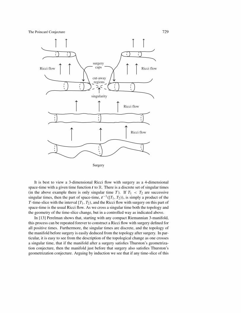
Suppose that we have a 3-dimensional Ricci flow (M, g(t)), a ≤ t < T , goingsingular at time T < ∞. In his second preprint on Ricci flow [13], Perelman extendsthis flow past time T by constructing a Ricci flow with surgery. To do this he makesuse of the classification of finite-time singularities described above. At the singulartime T there is a limiting metric (possibly incomplete) defined on an open submanifold� ⊂ M . The ends of � are diffeomorphic to S2 × [0, 1), with metrics near any pointthat look like a rescaled version of a product of a round metric on S2 with the Euclideanmetric on the interval, and with the curvature tending to infinity as one approaches theend. Surgery consists in cutting off the ends of these tubes along one of the 2-spheresin the product structure and sewing in a 3-ball to construct a new compact Riemannian3-manifold (M ′, g(T )) which will be the time-slice of the Ricci flow with surgery attime T . One restarts the Ricci flow at time T using (M ′, g(T )) as the initial metric.This flow will go singular at some time T ′ > T . See the figure below.

6See appendix.


Ricci flow

surgery

cut-away

singularity

Ricci flow

Ricci flow

Ricci flowcaps

regions

Surgery

It is best to view a 3-dimensional Ricci flow with surgery as a 4-dimensionalspace-time with a given time function t to R. There is a discrete set of singular times(in the above example there is only singular time T ). If T1 < T2 are successivesingular times, then the part of space-time, t−1([T1, T2)), is simply a product of theT -time-slice with the interval [T1, T2), and the Ricci flow with surgery on this part ofspace-time is the usual Ricci flow. As we cross a singular time both the topology andthe geometry of the time-slice change, but in a controlled way as indicated above.

In [13] Perelman shows that, starting with any compact Riemannian 3-manifold,this process can be repeated forever to construct a Ricci flow with surgery defined forall positive times. Furthermore, the singular times are discrete, and the topology ofthe manifold before surgery is easily deduced from the topology after surgery. In par-ticular, it is easy to see from the description of the topological change as one crossesa singular time, that if the manifold after a surgery satisfies Thurston’s geometriza-tion conjecture, then the manifold just before that surgery also satisfies Thurston’sgeometrization conjecture. Arguing by induction we see that if any time-slice of this

730 John W. Morgan

Ricci flow with surgery satisfies Thurston’s geometrization conjecture, then so doesthe initial manifold.

10. Completion of the proof of the Poincaré Conjecture

Let M be a closed, simply connected 3-manifold. To prove the Poincaré Conjecturefor M , namely to prove that M is diffeomorphic to the 3-sphere, we shall show that itsatisfies Thurston’s geometrization conjecture, which means that it has a Riemannianmetric of constant positive curvature. From there, it is easy to see that it is diffeo-morphic to the 3-sphere. Fix any Riemannian metric g(0) on M . (Remember thereis an infinite dimensional space of possibilities.) Now construct the Ricci flow withsurgery defined for all time with (M, g(0)) as the 0 time-slice. As we noted above, ifwe can show that any time-slice of this Ricci flow satisfies Thurston’s geometrizationconjecture, then so does M . So the proof of the Poincaré Conjecture is completedby showing that the time-slices of this Ricci flow with surgery at all sufficiently largetimes are empty, that is to say the Ricci flow with surgery becomes extinct at somefinite-time, just as Hamilton showed for the Ricci flow in the case when the Riccicurvature is positive.

The special property that Perelman uses about a homotopy 3-sphere in [12] in orderto prove the above finite-time extinction result is the fact that its second homotopygroup vanishes and its third homotopy group is non-trivial. Associated to a non-trivial element in the third homotopy group of a Riemannian manifold is a geometricinvariant. This invariant is the area of a certain disk related to the homotopy element,so that in particular the invariant is always non-negative. On the other hand, Perelmanshows that as long as the Ricci flow with surgery starting with a homotopy 3-spheredoes not become extinct, the derivative of this invariant is bounded above by a functionthat eventually becomes negative and stays bounded away from zero. This means thatthe invariant would have to become negative in finite-time, if the Ricci flow withsurgery does not become extinct. This is impossible, showing that the Ricci flow withsurgery does become extinct in finite-time.

11. Status of the Geometrization Conjecture

It seems quite likely that one can apply the existence of a Ricci flow with surgery, start-ing with any compact manifold, to establish the complete classification of3-manifolds as posited by Thurston’s conjecture. For example, the arguments ofthe previous section apply to any prime manifold with non-trivial π2 or π3. TheRicci flow with surgery starting at such a manifold becomes extinct in finite time,and hence these manifolds satisfy Thurston’s conjecture. To classify all 3-manifolds,one must understand the nature of the limits as t tends to infinity of the t time-slices.In [13] Perelman, following similar earlier arguments of Hamilton, showed that for


all sufficiently large t the time t time-slice Mt of a Ricci flow with surgery containsa finite collection of tori (and Klein bottles) whose fundamental groups inject intothe fundamental group of Mt . Furthermore, the complementary components are oftwo general types: those of the first type admit a complete hyperbolic metric of finitevolume, and those of the second type are collapsed, in the sense that they are, locallyat least, metrically close to lower dimensional spaces, spaces of dimension 1 or 2. Tocomplete the proof of Thurston’s conjecture one must show that the complementarycomponents of the second type are unions of generalized circle bundles and 2-torusbundles where the union takes place along boundary tori whose fundamental groupinjects into the fundamental group of Mt .

Perelman has stated such a result at the end of [13], and there is a closely relatedresult in [16], which relies on an earlier, unpublished result of Perelman. The evidenceis quite strong that these arguments will withstand scrutiny, but it is still too early tosay that this result has been established.

12. Future applications of Perelman’s work

Ironically enough Perelman’s proof of the Poincaré Conjecture, and even the proofof the Geometrization Conjecture, assuming that it withstands scrutiny, will havelittle effect of 3-dimensional topology. Those working in the subject either werealready assuming these results were true, were working on hyperbolic 3-manifolds,where by definition Thurston’s conjecture holds, or were working on the properties ofvarious algebraic, combinatorial, and geometric invariants of 3-manifolds, invariantsthat seem, at the present moment, to have little to do with the classification of 3-mani-folds. I believe the deepest impact of Perelman’s work will lie elsewhere.

One obvious area where these ideas will have impact is in the area of 4-dimensionalmanifolds. We know much less about smooth 4-manifolds than we do about smooth3-manifolds, and there are many significant questions to face before there can be fullapplication of the Ricci flow techniques to the study of 4-manifolds. These questionsinclude the nature of Einstein 4-manifolds (the fixed points up to scaling of the Ricciflow), as well as an extension of the curvature pinching results of Hamilton and thecollapsing results of Perelman, et al., to four dimensions. Still, this is an area wherethere seems much possibility for future advances.

Another area, where progress is already being seen, is the area of the Kähler–Ricciflow – Ricci flow on Kähler manifolds. Here many of the analytic problems disappear,and there is much more understood about Ricci flow.

Lastly, and more speculatively, Perelman’s techniques give one strong control oversingularity development in the Ricci flow for compact 3-manifolds. There are manyevolution equations in both mathematics and in mathematical models of physicalphenomena that are evolution equations which share many properties with Ricci flow.Understanding of singularity development in these equations could have significantinfluence both in mathematics and in the study of physical phenomena.

732 John W. Morgan

These applications, however significant, lie in the future. What we are discussingtoday is a milestone – the application of Ricci flow and Perelman’s breakthroughs tothe proof of one of the most central and long-standing problems in mathematics. Thatalone is enough to demonstrate the power and originality of the techniques.

Appendix. Formal definitions

The fundamental group: For any topological space X with a chosen point, x ∈ X,called the base point, the fundamental group π1(X, x) is defined. The elements ofthis group are deformation classes of loops based at x. The multiplication is given bycomposing loops. The identity element of the group is the class of the trivial loop atthe base point and the inverse of the class of a loop is the class of the loop with thedirection reversed.

Topological and smooth manifolds. By definition every point in a topological n-manifold has a neighborhood that is homeomorphic to a neighborhood in Euclideann-space. Transferring the usual coordinates on Euclidean space by this homeomor-phism gives us local coordinates on this neighborhood of the point. Thus, every pointin a topological manifold has a neighborhood with local coordinates like those ob-tained by restricting the usual Euclidean coordinates to an open subset of Euclideann-space. If two coordinate systems overlap, then the coordinate functions in onesystem are continuous functions of the other coordinates. A smooth manifold orequivalently a smooth structure on a topological manifold is a choice of a subsetof coordinate systems covering the entire manifold so that when two of the chosencoordinate systems overlap, the coordinate functions of one system are infinitely dif-ferentiable functions of the other coordinates. Amazingly enough, Milnor’s resultsshow that starting in dimension 8, it is not always possible to find a smooth structureon a topological manifold, and starting in dimension 7 it is possibly to have non-isomorphic smooth structures on a topological manifold, in fact on the 7-sphere. Thework of Freedman [4] and Donaldson [3] show that the theory of smooth 4-manifoldsdiffers enormously from the theory of topological 4-manifolds.

Hyperbolic geometry. Hyperbolic space of dimension n can be thought of as then-dimension sphere of radius i, and hence of constant curvature −1. The solutions tothe equation

−x20 + x2

1 + · · · + x2n = −1

in (n + 1)-space form a two-sheeted hyperboloid. Hyperbolic n-space is the uppersheet of this hyperboloid, i.e., the intersection of this locus with {x0 > 0}. Its groupof isometries is the subgroup of index two of the automorphism group preserving thequadratic form Q(x0, . . . , xn) = −x2

0 + x21 + · · · + x2

n preserving the two-sheets.Hyperbolic manifolds are obtained by taking the quotient of hyperbolic space bydiscrete subgroups of the isometry group that act freely on hyperbolic space.


Homogeneous 3-dimensional manifolds. Homogeneous 3-dimensional manifoldsare by definition 3-dimensional manifolds of the form G/H where G is a connectedLie group and H ⊂ G is a compact, connected subgroup. For example, S3 is homoge-nous because it can be written as the quotient Spin(4)/Spin(3). Hyperbolic space ofdimension three, is written as the quotient SL(2, C)/ SU(2). There are 9 possibilitiesthat lead to 3-dimensional quotients. A locally homogeneous manifold is then thequotient of G/H by a discrete subgroup � ⊂ G that acts freely on G/H . We are onlyconcerned with those G/H that admit cofinite volume discrete subgroups �. Thisleaves only 8 three-dimensional examples. The most interesting locally homogeneous3-manifolds are the hyperbolic ones. All others are easily classified and give fairlysimple examples.

Cutting apart 3-manifolds, Part I: The prime decomposition. Let X and Y beconnected, oriented 3-manifolds. The connected sum of X and Y , denoted X # Y isformed by removing from each of X and Y an open 3-ball and then identifying theboundary two-spheres, to create a new 3-manifold. Notice that if X is homeomorphicto the 3-sphere, then X # Y is homeomorphic to Y . A connected sum decompositionof a 3-manifold M is an equivalence between M and a connected sum X # Y . Bydefinition, it is a non-trivial connected sum decomposition if and only if neither X

nor Y is homeomorphic to the 3-sphere. A 3-manifold is prime if it does not admita non-trivial connected sum decomposition. It is a theorem of Kneser’s from the1920s that every 3-manifold can be decomposed as a finite connected sum of primemanifolds, and a result due to Milnor shows that this decomposition is unique up tothe order of the pieces. The first step in Thurston’s Conjecture is to decompose ageneral compact 3-manifold into its prime pieces. This is achieved by cutting the3-manifold open along a finite collection of disjoint 2-spheres and capping off theresulting 2-sphere boundaries with 3-balls. Of course, in general this process willproduce a disconnected manifold from a connected one.

Cutting apart 3-manifolds, Part II: The decomposition along tori. Thurston’sConjecture states that every prime 3-manifold can further be decomposed along adisjoint family of tori and Klein bottles (each of which has fundamental group injectinginto the fundamental group of the 3-manifold) so that each open complementarycomponent admits a complete, locally homogeneous metric of finite volume.

Curvature and covariant derivatives. There is another way to view the Riemanncurvature tensor. A Riemannian metric produces a way to differentiate tensors on themanifold, called covariant differentiation. If X is a vector field on the manifold thencovariant differentiation in the X direction is denoted ∇X. Briefly, there are two typesof conditions that determine the covariant differentiation associated to a metric. Thefirst are general rules for covariant differentiation in contexts much more general thanthis one. They are:

(1) The pairing of vector fields (X, Y ) �→ ∇XY is bilinear over the scalars (R).

734 John W. Morgan

(2) The pairing in the first item is linear over the smooth functions in the firstvariable:

∇f XY = f ∇XY.

(3) The pairing in the first item satisfies a Leibniz rule in the second variable:

∇X(f Y ) = f ∇XY + X(f )Y,

where X(f ) is the usual differentiation of the function f by the vector field X.

The rest of the rules relate the covariant differentiation determined by a Riemannianmetric to that metric and to the Lie bracket of vector fields. They are:

(4) Covariant differentiation preserves the metric in the sense that for all vectorfields X, Y , Z we have

X〈Y, Z〉 = 〈∇XY, Z〉 + 〈X, ∇Y Z〉,where the brackets denote the inner product coming from the metric.

(5) The covariant derivative is symmetric in the sense that ∇XY −∇Y X = [X, Y ],where [ · , ·] is the usual Lie bracket of vector fields.

We then examine the extent to which the usual commutation rules fail for covariantdifferentiation in the coordinate directions. That is to say, suppose that we have localcoordinates (x1, . . . , xn) on the Riemannian manifold and denote by ∂i the (local)vector field ∂/∂xi , in the ith-coordinate direction. Then the failure of the usualcommutativity is given by

Rij = ∇∂i∇∂j − ∇∂j ∇∂i

.

Then Rij acts on vector fields so that we can form

Rijkl = 〈Rij ∂l, ∂k〉.Here, the inner product is the one determined by the metric between the pair of vectorfields. Also notice that reversal of indices between the two sides of the expression. Thereason for this is to make the sphere have positive rather than negative curvature. Thenwe have the symmetry properties of Rijkl : skew-symmetric in the first two variablesand in the last two variables, and symmetric under interchange of variables 1 and 2with 3 and 4.

There are many ways to view this tensor, but one of the most fruitful is to makeuse of all the symmetries described above and thus to consider it as a symmetricbilinear pairing on the second exterior power of the tangent bundle of the manifold.The associated quadratic form associates a real number to every two-dimensionalsubspace in the tangent plane to the manifold at a point. This number is the sectionalcurvature in the two-plane direction at the point. These sectional curvatures arethe analogues of the Gauss curvature for surfaces. Of course, using the metric we


can transform this symmetric bilinear pairing to a symmetric endomorphism of thesecond exterior power of the tangent bundle, and that is another useful way to viewthe Riemann curvature tensor. In the case of a surface, the Riemann curvature tensoris equivalent to the Gauss curvature.

Volume non-collapsing. Suppose that we have a Ricci flow (M, g(t)) on an n-dimensional manifold, and a point p ∈ M . The curvature scale at (p, t) is the largestr > 0 such that the norm of the Riemann curvature tensor is bounded by r−2 on theball of radius r in (M, g(t)) centered at p, denoted B(p, t, r), for all the metrics g(t ′)for t ′ ∈ [t−r2, t]. Fix a positive constant κ . We say that (M, g(t)) is κ-non-collapsedon the scale of its curvature at (p, t) if for r equal to the curvature scale at (p, t) wehave Vol B(p, t, r) ≥ κrn.

References

[1] Browder, William, Surgery on simply-connected manifolds. Ergeb. Math. Grenzgeb. 65,Springer-Verlag, New York 1972.

[2] Cao, H. D., Chow, B., Chu, S. C., and Yau, S. T., (eds.), Collected papers on Ricci flow,Series in Geometry and Topology 37, International Press, Somerville, MA, 2003.

[3] Donaldson, S. K., Smooth 4-manifolds with definite intersection form. In Four-manifoldtheory (Durham, N.H., 1982), Contemp. Math. 35, Amer. Math.Soc., Providence, RI, 1984,201–209.

[4] Freedman, Michael Hartley, The topology of four-dimensional manifolds. J. DifferentialGeom. 17 (3) (1982), 357–453.

[5] Gray, Jeremy, A history of prizes in mathematics. In The Millennium Prize Problems, ClayMathematics Series, Amer. Math. Soc., Providence, RI, 2006, 3–30.

[6] Hamilton, Richard S., Three-manifolds with positive Ricci curvature. J. Differential Geom.17 (2) (1982), 255–306.

[7] Hilbert, David, Mathematical problems. Bull. Amer. Math. Soc. (N.S.) 37 (4) (2000),407–436; reprinted from Bull. Amer. Math. Soc. 8 (1902), 437–479.

[8] Milnor, John, On manifolds homeomorphic to the 7-sphere. Ann. of Math. (2) 64 (1956),399–405.

[9] Milnor, John, Towards the Poincaré conjecture and the classification of 3-manifolds. No-tices Amer. Math. Soc. 50 (10) (2003), 1226–1233.

[10] Papakryiakopoulos, C. D., On Dehn’s lemma and the asphericity of knots. Proc. Nat. Acad.Sci. U.S.A 43 (1957), 169–172.

[11] Perelman, Grisha, The entropy formula for the Ricci flow and its geometric applications.Preprint, 2002; arXiv:math.DG/0211159.

[12] Perelman, Grisha, Finite extinction time for the solutions to the Ricci flow on certainthree-manifolds. Preprint, 2003; arXiv:math.DG/0307245.

[13] Perelman, Grisha, Ricci flow with surgery on three-manifolds. Preprint, 2003;arXiv:math.DG/0303109.

736 John W. Morgan

[14] Poincaré, Henri, Cinquième complément à l’analysis situs. In Œuvres. Tome VI, reprint ofthe 1953 edition, Grands Class. Gauthier-Villars, Éditions Jacques Gabay, Sceaux 1996.

[15] Scott, Peter, The geometries of 3-manifolds. Bull. London Math. Soc. 15 (5) (1983),401–487.

[16] Shioya, Takashi, and Yamaguchi, Takao, Volume collapsed three-manifolds with a lowercurvature bound. Math. Ann. 333 (1) (2005), 131–155.

[17] Smale, Stephen, Generalized Poincaré’s conjecture in dimensions greater than four. Ann.of Math. (2) 74 (1961), 391–406.

[18] Stallings, John, A topological proof of Gruscho’s theorem on free products. Math. Z. 90(1965), 1–8.

[19] Thurston, William P., Hyperbolic structures on 3-manifolds. I. Deformation of acylindricalmanifolds. Ann. of Math. (2) 124 (2) (1986), 203–246.

[20] Waldhausen, Friedhelm, On irreducible 3-manifolds which are sufficiently large. Ann. ofMath. (2) 87 (1968), 56–88.

Mathematics Department, Columbia University, 2990 Broadway, New York, NY 10027,U.S.A.E-mail: [email protected]

the poincar© conjecture - icm 2006

Documents