the political economy of debt and entitlements · the political economy of debt and entitlements...
TRANSCRIPT

The Political Economy of Debt and Entitlements�
Laurent Boutony Alessandro Lizzeriz Nicola Persicox
August 12, 2016
Abstract
This paper presents a dynamic political-economic model of total government oblig-
ations. Its focus is on the interplay between debt and entitlements. In our model, both
are tools by which temporarily powerful groups can extract resources from groups that
will be powerful in the future: debt transfers resources across periods; entitlements
directly target the future allocation of resources. We prove �ve main results. First,
debt and entitlement are strategic substitutes in the sense that constraining debt in-
creases entitlements (and vice versa). Second, if entitlements are unconstrained, it
is sometimes bene�cial not to constrain debt (even in the absence of shocks that re-
quire smoothing). Third, if debt is unconstrained, it is bene�cial to limit entitlements
but not to eliminate them. Fourth, debt and entitlements respond in opposite ways
to political instability and, in contrast with prior literature, political instability may
even reduce debt when entitlements are endogenous. Finally, we identify a possible
explanation for the joint growth of debt and entitlements.
JEL Classi�cation: D72, E62, H60
Keywords: Government debt, entitlement programs, �scal rules, political economy
�We thank Marina Azzimonti, Micael Castanheira, Pedro Gete, and Stefanie Stantcheva.yDepartment of Economics, Georgetown University, and ECARES, Université libre de Bruxelles. E-
mail: [email protected] of Economics, NYU. E-mail: [email protected] School of Management, Northwestern University. E-mail: [email protected]

1 Introduction
Increasingly, governments are struggling to meet their �scal obligations. Fiscal stress is
usually blamed on government debt; but governments have other spending obligations
that, like interest payments, are di¢ cult to compress, most notably pensions and health
care. Because these programs can be di¢ cult to renegotiate, in the US they are referred
to as entitlements.
Entitlements are a major determinant of �scal sustainability in many jurisdictions
because they are large (on a �ow basis, larger than interest payments on debt) and because
by de�nition they cannot easily be compressed. Sometimes entitlements are practically
the sole determinant of �scal sustainability: this is the case for some US states where debt
is strictly capped by state constitutions. In comparative terms, in the U.S. entitlements
have grown rapidly since the 1960s and have overtaken discretionary spending, suggesting
that entitlement programs must be crowding out other types of government spending
such as, perhaps, infrastructure and R&D spending.1 ;2 A similar pattern in the growth of
entitlements holds across OECD countries.3
Leading academics have long pointed out that debt and entitlements should be recog-
nized as a combined burden from an accounting perspective (see Kotliko¤ and Burns,
2004). On occasion, this accounting fungibility has even been made explicit through policy
choices.4 Accordingly, the European Commission has recently developed a forward-looking
measure of �scal sustainability, the �intertemporal net worth,�that captures government
obligations much more broadly than simple measures of debt.5 But despite this recogni-
tion in the policy world and at the level of measurement, there is no academic work that
studies the political forces that jointly shape debt and entitlements.
In this paper we provide a politico-economic model in which debt and entitlement levels
1See, e.g., Steuerle (2014) and David Crane: �New California Taxes Pay for Pensions, Not Students.�Bloomberg, April 23 2012.
2Another way to illustrate this evolution is to look at the Steuerle and Roeper index of Fiscal Democracythat measures the percentage of (projected) revenues not claimed by permanent programs currently inplace. In the US, this index dropped from 65% in 1962 to a range between 0 and 20 percent in the period1998-2012; it is forecast to stay in this range through 2022, and there is no expectation of improvementin the more distant future. See Steuerle (2014). Evans, Kotliko¤, and Phillips (2012) provide anothermeasure of �scal sustainability �the so-called duration to game over. In the case of the US, this measurealso points to the high (or even unsustainable) �scal burden of entitlement programs.
3De�ned as: public social expenditure as a percent of GDP in 1960-2014. Source: OECD (2014).4�Chile performed such a greased swap in 1980. [...] It took back pension promises from workers in
exchange for government bonds plus a kicker. Argentina, Bolivia, and Hungary have forcefully con�scatedprivate pension assets (largely government bonds), swapping them for larger future pension commitments.�Newsweek, January 15 2015.
5 Intertemporal Net Worth is based on the total discounted sum of future primary balances undercurrent policies and current net worth. This measure suggests that assessing the �scal burden via debt onlyand ignoring entitlements not only severely understates the problem but can also bring about misleadinginferences about the relative burden across countries. For instance, according to some of these measuresthe EU country in the best state of �scal health is Italy, despite its extremely high level of governmentdebt.
2

are jointly determined in equilibrium. Because we aim to keep our analysis comparable
with the previous literature, our starting point is a slight variant on the canonical politico-
economic model by Alesina and Tabellini (1990), which focuses on debt only. Absent
entitlements, our model replicates key results in the debt-only models by Persson and
Svensson (1989) and by Alesina and Tabellini (1990). We then allow for the coexistence
of debt and entitlements. The resulting model allows us to study the interplay between
debt and entitlements and thus to investigate the political economy of total government
obligations.
The key ingredients of the model are the following. In each period, a political process
determines spending on a public good as well as private goods for two groups. Political
power changes over time, as for instance in an intergenerational setting. The currently
powerful groups (we call these �group A�) can use debt to leverage future resources to
�nance higher current consumption. In addition, group A can set entitlements, i.e., �pre-
commit� some fraction of future resources to a desired allocation. Thus, in our model
both debt and entitlements are tools for temporarily powerful groups to extract resources
from groups that will be more powerful in the future (we call these �group B�).
This way of modeling entitlements is consistent with Schick�s de�nition (2009, p. 2-3):
an entitlement is a provision of law that establishes a legal right to public funds for a class
of citizens. A further characteristic of entitlements is that they have proved di¢ cult to
change without the bene�ciaries�consent.6 In the vast majority of US states, for example,
changing future bene�ts for current employees is extremely di¢ cult.7 And across the
world, even when pension laws have been revised, the bene�ts of current retirees have
generally been protected. We discuss the mechanisms that protect entitlements in Section
9.5, but in our model we simply assume that entitlements cannot be changed without the
bene�ciaries�consent.
Our results are the following. We �rst characterize the equilibrium level of debt and
entitlements. We show that, while absent entitlements debt is always positive, in the
presence of endogenous entitlements debt levels are reduced to an extent that group A
may choose to run a surplus. Nevertheless, we show that the presence of entitlements leads
to an increase of total government obligations compared to the case of zero entitlements.
Furthermore, entitlements allow group A to smooth its private consumption over time but
they crowd out period-2 public consumption.
We then show that debt and entitlement are strategic substitutes in the sense that
constraints on debt lead to increases in entitlements (and vice versa). This result has direct
6Schick (2009, p. 2-3). �The government (or the social security fund) is obligated to pay the amount towhich recipients are entitled whether or not su¢ cient funds have been set aside for this purpose in the bud-get. In many countries, a permanent appropriation �nances social security and various other entitlementprogrammes. But even when the entitlement is �nanced by annual appropriations, the government mustprovide the bene�ts mandated by law.�For US federal spending, entitlements can be de�ned precisely asgovernment spending that is mandatory �that is, not subject to appropriation.�
7Munnell and Quinby (2012).
3

implications for the evaluation of policies implementing debt limits�e.g., the so-called
balanced budget rules that have long existed in many US states�and more generally, for
the �scal rules that are increasingly prevalent across many countries.8 These policies may
have the unintended (and hard-to-measure) consequence of increasing entitlements. This
could in turn dramatically reduce the e¤ect of those limits on total government obligations.
We argue that our analysis has implications for the empirical literature studying the e¤ect
of �scal rules (Poterba 1996, Alesina and Perotti 1999, Badinger and Reuter 2015).
We then evaluate the welfare consequences of �scal rules in the presence of endogenous
entitlements. We show that relaxing balanced-budgets requirements may lead to Pareto
improvements even in the absence of any tax-smoothing motive driven by economic shocks.
This is because debt helps reduce the socially excessive use of entitlements. This is in
contrast with prior work where, absent aggregate shocks, debt is always excessive and hence
debt limits are bene�cial. We then consider the utilitarian-welfare e¤ects of constraining
entitlements. We show that, if debt is unconstrained, it is bene�cial to limit entitlements
but not to eliminate them. Entitlements are socially useful because they allow consumption
smoothing for group A. Yet, because in equilibrium group A extracts too much from group
B, it is socially bene�cial to reduce group A�s extractive ability, implying that a limit to
entitlements is bene�cial.
We then explore how equilibrium levels of debt and entitlements respond to changes in
the persistence of political power, or its opposite, government instability. This exploration
is motivated by prior literature that provides compelling reasons to think that debt de-
creases as political power becomes more persistent.9 This result can be reproduced in our
environment when we do not allow for entitlements. However, we show that predictions
become more nuanced if entitlements are endogenous. Speci�cally, we show that debt and
entitlements move in opposite directions when persistence increases. Furthermore, debt
sometimes increases with persistence�and even more surprisingly, the total �scal burden
(debt plus entitlements) may increase with persistence. This is a rich set of empirical
implications that could in principle be tested in cross-country data, as was done for the
Alesina-Tabellini model by Ozler and Tabellini (1991), Crain and Tollison (1993), Franzese
(2002), and Lambertini (2003).
Finally, we study potential factors that may explain the joint growth of debt and enti-
tlements in the past decades. In most OECD countries, �scal pressure has been ratcheted
up by the simultaneous growth in debt and entitlements. That these two aggregates should
grow together is intriguing, because it is natural to think of debt and entitlements as sub-
stitute tools of intergenerational redistribution. Yet under some conditions, our model
predicts that debt and entitlements are comonotonic, meaning that as some underlying
8The number of countries with at least one �scal rule has grown from �ve in 1990 to 80 in 2012 (seeSchaechter et al. 2012).
9The logic is that debt is issued by the currently politically powerful only when they fear losing powerin the future (see the seminal work of Alesina and Tabellini 1990).
4

features of the environment change, debt and entitlements move together. For instance,
we show that an increase in generational con�ict may lead to an increase in both debt and
entitlements.
2 Related Literature
Some papers explain debt as the outcome of a struggle between di¤erent groups in the
population who want to gain more control over resources. The reason debt is accumulated
is that the group that is in power today may not be in power tomorrow, and debt is a way
to take advantage of this temporary power. For instance, Cukierman and Meltzer (1989)
and Song, Storesletten, and Zilibotti (2012) argue that debt is a tool used to redistribute
resources across generations. Persson and Svensson (1989), Alesina and Tabellini (1990),
and Tabellini and Alesina (1990) argue that debt represents a way to tie the hands of future
governments that will have di¤erent preferences from the current one. In Tabellini and
Alesina (1990), voters choose the composition of public spending in an environment where
the median voter theorem applies. If the median voter remains the same in both periods,
the equilibrium involves budget balance. If the median voter tomorrow has di¤erent
preferences, the current median voter may choose to run a budget de�cit to take advantage
of his temporary power and tie the hands of the future government. The equilibrium may
also involve a budget surplus because there is an �insurance�component that links the two
periods as well: a surplus tends to equalize the median voter�s utility in the two periods.
Tabellini and Alesina (1990) detail conditions such that de�cits will be incurred and show
that increased polarization leads to larger de�cits.
Browning (1975) and Boadway and Wildasin (1989) have studied voting models of pen-
sions in which age is the only dimension of heterogeneity. Conde-Ruiz and Galasso (2005)
study a two-dimensional voting model in which pensions coexist with a welfare state. Thus
they allow for voting on both intragenerational and intergenerational redistribution. They
argue that pensions are particularly stable because the elderly are a relatively homoge-
neous voting group, and the pension system is supported by a broad coalition including
the low-income young.
Tabellini (1991) also illustrates how debt and social security di¤er as distributional
instruments in an overlapping generations environment. In contrast with our model, the
main force concerns the di¤erence in default between the two instruments.
Battaglini and Coate (2008) present a dynamic model of taxation and debt where
a rich policy space is considered within a legislative bargaining environment. Velasco
(1996) discusses a model where government resources are �common property�with which
interest groups can �nance their own consumption. De�cits arise in his model because of
a dynamic �common pools�problem. Lizzeri (1999) presents a model of debt as a tool of
redistributive politics.
5

The dynamic public �nance literature (e.g., Golosov, Tsyvinski and Werning 2006)
provides a setup that is suited to the normative study of debt and entitlements, although
this question has not been a main substantive focus of this literature so far.10
This paper is also related to work on legislative bargaining with endogenous status quo.
Kalandrakis (2004) studies a classic divide-the-dollar problem where the division agreed to
in one period is the status quo for the next period. Bowen, Chen and Eraslan (2014) study a
model in which two parties decide unanimously how to allocate a given budget to spending
on a public good and private transfers. The focus is on the comparison between two
political institutions: discretionary vs. mandatory public good spending (private transfers
are discretionary in both cases).11 When the public good is discretionary (mandatory),
the status quo level of the public good is zero (the one from the previous period). By
contrast, we focus on the interplay between debt and entitlements.
A very di¤erent approach to understanding public debt is explored by Azzimonti et al.
(2014). They propose a multi-country model with incomplete markets, and they show that
governments may choose higher public debt when �nancial systems are more integrated.
They thus o¤er an explanation of the rise in debt as driven by an increase in �nancial
integration. Related to our discussion of the comovement of entitlements and debt, they
also show that debt increases with the level of idiosyncratic risk.
3 Model
In this section we present the model. Section 9 provides a discussion of some of the
assumptions.
3.1 Demography and economy
There are two groups, A and B, who each live for two periods. In each period t there is
an endowment of 1 that can be allocated to private goods for the two groups xtA and xtB,
or to a public good gt. Preferences in each period are given by:
ui�xti; x
tj ; g
t�= h
�xti�+ v
�gt�;
where h (�) and v (�) are concave, and twice continuously di¤erentiable. We also assumethat both the private and the public goods are su¢ ciently valuable that h0 (0) = 1 =
v0 (0), implying that it is not optimal for one group to spend all the resources on its own
private good or on the public good. Utility is additive across periods and there is no
10See also Stantchveva (2014) and (2016). Regarding the latter, one could think of entitlements aspromised spending on education and health.
11 In a modi�ed version of this model�with two periods and no private transfers�Bowen et al. (2015)allow the party making the take-it-or-leave-it o¤er to choose whether the public good is discretionary ormandatory. The focus is on the e¢ ciency of the public good provision under various budgetary institutions.
6

discounting. There are no capital markets to either privately save or borrow.12
The resource constraints in periods 1 and 2 are given by:
x1A + x1B + g
1 � 1 + d
x2A + x2B + g
2 � 1� d;
where d represents debt or surplus, and the interest rate is assumed to be zero. We assume
xtA; xtB; g
t � 0, and thus d 2 [�1; 1] :We assume no default on debt, but we revisit this assumption in Section 9.5.4.
3.2 Political structure and entitlements
Except for Section 7, throughout the paper the political structure is such that group A
decides the allocation in period 1; group B decides the allocation in period 2 subject to
debt and entitlements, as speci�ed below.
In period 1, group A chooses the quintuple:
�x1A; x
1B; g
1; d; E�;
subject to the resource constraint. E is a nonnegative number that represents group A�s
entitlements in the future. In period 2, group B chooses the triple:
�x2A; x
2B; g
2�;
subject to the resource constraint and to the additional constraint that entitlements need
to be honored:
x2A � E:
Note that like debt, entitlements (E) are placed beyond group B�s political ability to
renegotiate.
4 Equilibrium Analysis
In this section, we start with some preliminary analysis that are necessary for our charac-
terization of equilibrium policies. We denote by c the portion of the second period budget
that has been already been committed (either in debt or entitlements) in period 1.
De�nition 1 (second-period policies) De�ne second-period policy choices conditional
12 In Section 9.2 we argue that the main results are unchanged if we allow for private savings as long asthere is some intertemporal friction such as a positive tax on capital.
7

on a budget commitment of c as the set X (c) ; G (c) that solves:
max(x;g)
h (x) + v (g) s.t. x+ g � 1� c:
X (c) represents the amount of private good that a group (either A or B, whichever
has the power to choose the allocation) would allocate itself in period 2, subject to the
constraint that a fraction c of period 2�s endowment has been reserved for other purposes.
G (c) represents the corresponding amount of public good.
Lemma 1 (well-behaved second-period policies) Second period policy choices X (c)and G (c) are single-valued di¤erentiable functions that are decreasing in c: Thus, increas-
ing the fraction of the second period budget which is committed lowers private and public
consumption in the second period.
Proof. See Appendix A.
In period 2, group B is in power. We can use De�nition 1 to describe group B�s
allocation choice.
Corollary 1 (second period equilibrium allocation) Assume the second period startswith pre-de�ned commitments d of debt and E of entitlements. Then in period 2 group B
allocates exactly E to group A�s private good, allocates X (d+ E) in private good to itself,
and allocates G (d+ E) to the public good.
Given period-2 policy choices, we can move to consideration of optimal policies in the
�rst period.
De�nition 2 (�rst-period policies) De�ne �rst-period policy choices as the set (x�; g�; d�; E�)that solves:
max(x;g;d;E)
h (x) + v (g) + h (E) + v (G (d+ E)) s.t. x+ g � 1 + d: (1)
The four-tuple (x�; g�; d�; E�)maximizes group A�s lifetime payo¤. This payo¤ is partly
accrued in period 1 (the �rst two addends in equation (1)) and partly in period 2 (the last
two addends in equation (1)). However, in period 2 group A does not directly control the
allocation; therefore, its private consumption in period 2 is given by the amount E it chose
in entitlements in the �rst period, and its amount of public consumption is determined by
whatever amount group B chooses to provide given the (uncommitted) resources available
in the second period.
8

In what follows, we assume that v (G (�)) is concave. This guarantees concavity of theproblem faced by group A. Because G (�) is endogenous, it is helpful to provide su¢ cientconditions on the primitives that ensure the desired property. This is the purpose of the
next result.
Lemma 2 (su¢ cient conditions for concavity) v (G (�)) is concave if G (x) is con-cave.
1. G (x) is concave if and only ifv00([v0]�1(x))h00([h0]�1(x))
is nonincreasing in x:
2. (symmetric case) G (x) is concave if h (x) = v (x) :
3. (proportional CRRA functions) G (x) is concave if v (x) is CRRA and h (x) = �v (x)
for � > 0.
4. (CRRA functions with di¤erent curvatures) Suppose v (x) = xp=p and h (x) = xq=q;
with p; q < 1: Then G (x) is strictly concave if and only if p < q:
Proof. See Appendix A.
Before proceeding to discuss the characterization of the �rst period allocation, and of
debt and entitlements, it is useful to obtain a benchmark result in which, as in the prior
literature, we do not allow for entitlements. We will then contrast this with the case in
which entitlements are allowed. A useful feature of our model is that, absent entitlements,
it behaves similarly to prior literature on debt, notably the literature following Alesina and
Tabellini (1990). In this literature, debt arises whenever the currently powerful generation
fears the loss of political power in the future.
Proposition 1 (No entitlement benchmark) Fix E � 0: Then in equilibrium:
1. Group A runs up debt in period 1, d�E=0 > 0;
2. Group A�s private consumption decreases between periods 1 and 2;
3. Public good provision decreases between periods 1 and 2.
Proof. See Appendix A.
To gain some intuition for this result, it is useful to examine the �rst order condition
determining debt. Equation (2) below is obtained by di¤erentiating the objective function
(1) with respect to d (and �xing E = 0):
h0 (x) = �v0 (G (d))G0 (d) : (2)
9

If group A were in charge in both periods, then the term G0 (d) would not appear. This
term captures the fact that an extra dollar left uncommitted to period 2 only increases
public consumption by G0 (d) < 1, the marginal amount chosen by group B, with the
remainder going to group B�s private consumption. We call the presence of this term the
crowdout e¤ect. The crowdout e¤ect gives an incentive to increase debt. There is also a
smoothing e¤ect that works as follows: because of concavity in the utility function, group
A wants to smooth consumption over time. If public consumption is smaller in period
2 (which must be the case when debt is positive), then the smoothing e¤ect gives an
incentive to decrease debt. The balance of the crowdout e¤ect and the smoothing e¤ect
determines the equilibrium level of debt.
Part 2 is immediate: group B has no incentive to allocate resources to group A�s private
consumption since it does not bene�t from doing so.
Part 3 follows directly from part 1: since debt is positive, there are fewer resources
e¤ectively available for consumption, hence less public good, in period 2 than in period 1.
The next result o¤ers an initial characterization of the equilibrium of the model when
entitlements are allowed.
Proposition 2 (Equilibrium characterization) In equilibrium:
1. Total government obligations are always positive and larger than in the case without
entitlements: d� + E� > d�E=0;
2. Group A does not fully commit period 2�s budget: d� + E� < 1;
3. Public consumption decreases between periods 1 and 2;
4. Group A�s private consumption is perfectly smoothed;
5. Group A may choose to run a surplus; for example, if h (x) = v (x) have a CRRA
form (x)1�� = (1� �) ; then group A runs a surplus if and only if � > 1:
Proof. See Appendix A.
Part 1 of Proposition 2 shows that allowing for entitlements increases government oblig-
ations. In our model both types of government obligations arise because in period 2 group
A lacks political control and understands that a fraction of any uncommitted dollar will be
diverted from public consumption to group B�s private consumption. Absent entitlements,
the only way to pre-commit period 2 dollars is to consume them today (by issuing debt).
But, due to the concavity of the utility function, group A would prefer to allocate (at least
some of) these period 2 dollars to its private consumption in period 2. This is exactly
what entitlements allow group A to do. This additional commitment channel raises the
value of committing period 2 dollars and therefore leads to larger government obligations.
10

Part 2 highlights the moderating role that the public good plays in our model. Group
A does not wish to commit the entirety of tomorrow�s resources, because this would lead
to zero public consumption. We believe that this feature of the model is realistic in that
one reason that current generations refrain from full �scal depredation is that they realize
that they will need some public goods when they are retired. These public goods can only
be provided if whoever is in power then is left with some uncommitted �scal capacity.
Part 3 indicates that the pre-commitment of period 2�s budget results in a reduction
in public good provision. This feature has an empirical counterpart in the crowding out
of discretionary expenditures that is associated with the increase in entitlements.
Parts 4 and 5 of Proposition 2 highlight the di¤erences with the no-entitlements bench-
mark. Absent entitlements, private consumption cannot be perfectly smoothed across
periods. This is because group A lacks any political control over how money is spent in
period 2, and group B has no incentive to provide private consumption for group A. By
contrast, the availability of entitlements in conjunction with debt allows group A control
over its own private consumption in period 2. Thus, the presence of entitlements allows for
better intertemporal resource allocation (part 4) and lessens the proclivity to accumulate
debt (part 5).13
As we did after Proposition 1 for the case without entitlements, it is useful to discuss
the forces determining debt and entitlements. The two key �rst-order conditions that
determine debt and entitlements are obtained by di¤erentiating the objective function (1)
with respect to E and d respectively:
h0 (E) = �v0 (G (d+ E))G0 (d+ E) ; (3)
h0 (x) = �v0 (G (d+ E))G0 (d+ E) : (4)
These equations illustrate the di¤erent roles of debt and entitlements. Group A uses
debt to smooth consumption over time and entitlements to smooth consumption over
types of goods in period 2. As in the model with a single �commitment instrument,�the
crowdout e¤ect gives an incentive to group A to increase government obligations; this e¤ect
pushes toward both higher debt and higher entitlements. The smoothing e¤ect, however,
is quantitatively di¤erent in terms of how it a¤ects debt, and qualitatively di¤erent in
terms of how it a¤ects entitlements.
Regarding debt, the smoothing e¤ect is ampli�ed by the presence of entitlements and
in fact still remains strong even when debt is zero: part of period 2 resources are pre-
committed to entitlements, and thus for any given level of debt, the imbalance in public
consumption between periods 1 and 2 is even more pronounced. To smooth public con-
13We wish to emphasize that the possibility of surplus is not of interest in itself. We view it as a usefulcontrast with the no entitlement benchmark. Of course, surplus is also a possibility in other politicaleconomy models of debt (e.g., Persson and Svensson 1989). However, this is due to di¤erences in theutility functions between groups.
11
sumption across periods, group A may therefore choose to run a surplus.
Regarding entitlements, the smoothing e¤ect can be either positive or negative because
entitlements may be either lower or higher than public consumption depending on the
degree of risk aversion and on the relative importance of public consumption. In contrast,
in the case of debt, the sign of the smoothing e¤ect is always negative because public
consumption is always lower in the second period.
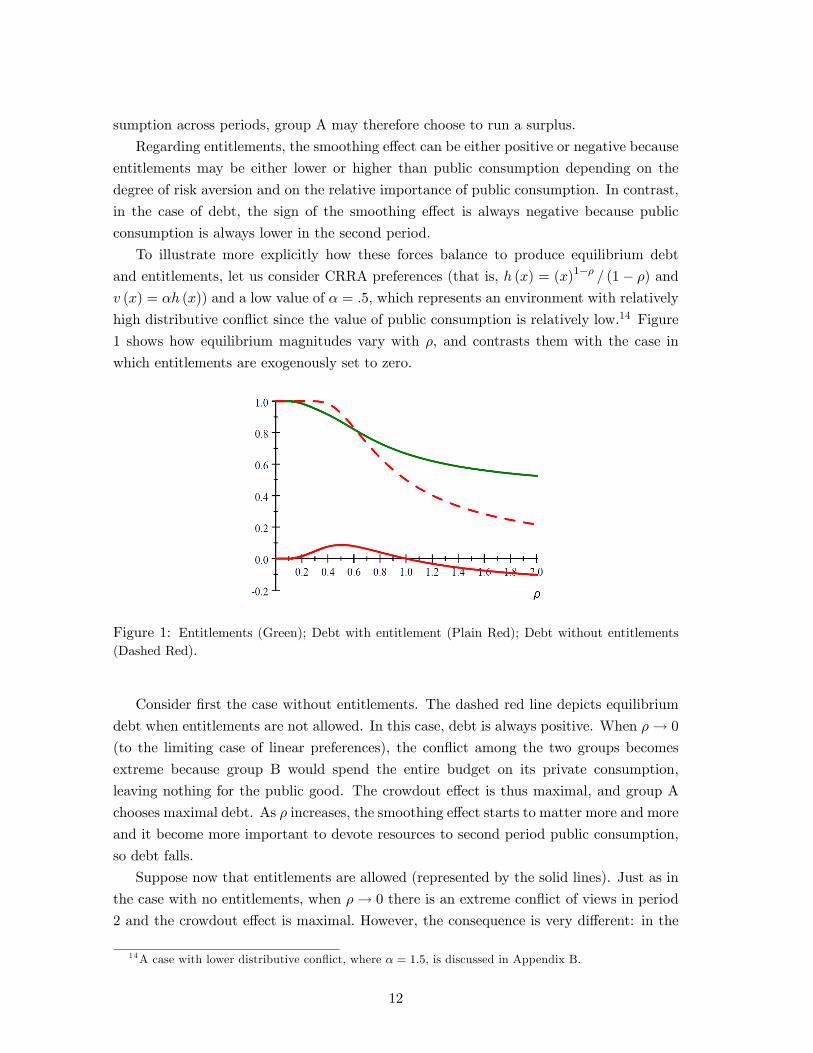
To illustrate more explicitly how these forces balance to produce equilibrium debt
and entitlements, let us consider CRRA preferences (that is, h (x) = (x)1�� = (1� �) andv (x) = �h (x)) and a low value of � = :5, which represents an environment with relatively
high distributive con�ict since the value of public consumption is relatively low.14 Figure
1 shows how equilibrium magnitudes vary with �, and contrasts them with the case in
which entitlements are exogenously set to zero.
Figure 1: Entitlements (Green); Debt with entitlement (Plain Red); Debt without entitlements(Dashed Red).
Consider �rst the case without entitlements. The dashed red line depicts equilibrium
debt when entitlements are not allowed. In this case, debt is always positive. When �! 0
(to the limiting case of linear preferences), the con�ict among the two groups becomes
extreme because group B would spend the entire budget on its private consumption,
leaving nothing for the public good. The crowdout e¤ect is thus maximal, and group A
chooses maximal debt. As � increases, the smoothing e¤ect starts to matter more and more
and it become more important to devote resources to second period public consumption,
so debt falls.
Suppose now that entitlements are allowed (represented by the solid lines). Just as in
the case with no entitlements, when �! 0 there is an extreme con�ict of views in period
2 and the crowdout e¤ect is maximal. However, the consequence is very di¤erent: in the
14A case with lower distributive con�ict, where � = 1:5, is discussed in Appendix B.
12

limit there is no debt and full entitlements. Entitlements are a superior way to capture the
second period resources as long as � > 0. Just as before, when � increases the smoothing
e¤ect implies that it becomes more desirable to devote part of the budget to the public
good, so entitlements drop. Debt responds non-monotonically to an increase in �. While
resources become available for the public good over both periods, the amount invested in
the public good is di¤erent in the two periods; for low values of �, the crowdout e¤ect
dominates, and for high values of � the smoothing e¤ect dominates.
5 Strategic Substitutes Property
We now discuss the relation between debt and entitlements. The next proposition estab-
lishes that the e¤ects of tightening a debt ceiling are partly (but not fully) o¤set by a
strategic adjustment in entitlements�and viceversa, that the e¤ects of constraining enti-
tlements are partly (but not fully) o¤set by a strategic increase in debt.
Proposition 3
1. (strategic substitutes property) Fix debt at a level d: The entitlement level E�d�
that maximizes group A�s lifetime utility conditional on d is a decreasing function of
d;
2. (strategic substitutes property) Fix entitlements at a level E: The debt leveld�E�that maximizes group A�s lifetime utility conditional on E is a decreasing
function of E;
3. (debt ceilings are partially e¤ ective) Tightening a binding debt ceiling d reducesd+ E
�d�, the sum of debt and entitlements in equilibrium;
4. (entitlement caps are partially e¤ ective) Tightening a binding cap on entitle-ments E reduces d
�E�+ E, the sum of debt and entitlements in equilibrium.
Proof. See Appendix B.
To understand the mechanism at work in part 1 (which also applies to part 2), imagine
that group A is constrained and can only run debt up to d. This may be because of a
�scal rule or for other reasons. Imagine now that the �scal rule is relaxed. The relaxation
causes a reduction in group B�s �scal capacity in the second period, and therefore a
reduction in public-good spending in that period. This reduction raises the marginal cost
of entitlements for group A.
Parts 3 and 4 show that, despite the partial crowding out, constraining either debts or
entitlements still reduces the total obligations that group A bequeaths to group B.
Despite its simplicity, Proposition 3 has a number of important implications.
13

First, consider the important literature that has highlighted the role of debt as an
instrument that perpetuates temporary power (e.g., Alesina and Tabellini 1990, Tabellini
and Alesina 1990, Persson and Svensson 1989).15 If, consistent with this literature, entitle-
ments were left out of our model (i.e., implicitly set to zero), Proposition 3 part 2 indicates
that the equilibrium level of debt would be larger than if entitlements were accounted for
by the model. That is, by abstracting from the presence of entitlements, there is a risk
of over-estimating the amount of debt that is created in an e¤ort to take advantage of
temporary power. Note however, that from Proposition 2 part 1 a model that abstracts
from entitlements would underestimate the total level of government obligations (i.e., the
sum of debt and entitlements).
Second, Proposition 3 has consequences for the evaluation of �scal constitutions. For
instance, the implementation of �scal rules or debt ceilings may have the unintended (and
di¢ cult-to-measure) consequence of increasing entitlements, thus partially o¤setting the
reduction in debt. By the same token, implementing pension reforms will make it harder to
stabilize government debt. This latter trade-o¤ seems con�rmed by the current structure
of the EU�s Stability and Growth Pact, a �scal rule that binds EU states. In 2005, it was
agreed that the spending ceiling enacted by the Pact would be relaxed for countries that
implemented structural reforms. As in our Proposition 3, structural reform and de�cit
reduction are treated as strategic substitutes.
Third, the result yields a testable implication: entitlements should be larger where
balanced-budget rules are more stringent.16 This speaks to the literature exploring the
e¤ects of �scal rules (Poterba 1996, Alesina and Perotti 1999, Badinger and Reuter 2015).
6 Welfare E¤ects of Constraining Debt or Entitlements
Absent entitlements, in our model, debt is harmful from the perspective of utilitarian
social welfare: there is no insurance motive (no shock, recession, war, or natural disaster)
in the model that could make debt desirable from the perspective of a utilitarian social
planner. In this section we study the welfare e¤ects of �scal rules constraining debt or
entitlements in our setting, where policies are not set by the social planner but emerge
endogenously from the political process.
We start with debt. The following proposition shows that, due to the endogenous
response of entitlements to tightening debt constraints, the welfare e¤ect of introducing
such constraints can be quite di¤erent than in a model without entitlements.
Proposition 4 (welfare e¤ ects of constraining debt).15This determinant of debt is a major component of recent developments in the political economy theory
of public debt (see, e.g., Battaglini and Coate 2008, Battaglini 2011, and Azzimonti et al. 2015).16A suggestive piece of prima facie evidence comes from the interaction between entitlements (proxied
by the percentage of pensions unfunded)and the stringency of balanced-budget rules in US states (asmeasured by Hou and Smith 2006). The correlation between the two is indeed positive (0.173).
14

1. Suppose debt is unconstrained and h (x) = v (x) have a CRRA form (x)1�� = (1� �).There is a �̂ such that introducing a barely-binding debt cap leaves group A indi¤erent
at the margin; group B is made strictly better o¤ if � > �̂ and strictly worse o¤ if
� < �̂;
2. For some parameter con�gurations, relaxing a binding constraint on debt is a strict
Pareto improvement: for example, if h (x) = v (x) have a CRRA form (x)1�� = (1� �) ;then relaxing a binding constraint on debt makes both groups A and B better o¤ at
the margin if � < �̂:
Proof. See Appendix C.
The intuition of part 1 of Proposition 4 is as follows. A marginal constraint on debt
transfers resources from period 1 to period 2. This increases group B�s utility in period 2
(total obligations go down, thus available resources to group B go up), but decreases it in
period 1 (debt goes down, hence public good provision). To understand the net welfare
e¤ect, note that (i) group B�s marginal utility of consumption is higher in period 2 than in
period 1 (because public good provision is higher in the second period), and (ii) due to the
endogenous reaction of entitlements to a change in debt, only a portion of the resources
transferred to period 2 bene�t group B. Thus, the net welfare e¤ect for group B is positive
if the di¤erence in marginal utility across periods is su¢ cient to compensate for the �loss�
in resources.
Proposition 4 part 2 is rather intriguing. Despite the fact that debt is used by group
A as a tool to expropriate group B, in equilibrium, allowing more debt can be socially
bene�cial. A central driver for Proposition 4 part 2 is the fact that, in our model, resources
are used less e¢ ciently in period 2 than in period 1. Indeed, group A chooses the level of
entitlements, taking into account that only a fraction of the remaining budget in period 2
will be devoted to the public good by group B. As a consequence, group A entitles itself
excessively (from a social perspective). By decreasing the budget in period 2, debt helps
reduce that ine¢ ciency. However, of course, increasing debt also has a cost: it leads to
a decrease in other types of consumption in period 2. This is particularly costly from
a utilitarian perspective because group 2 receives lower consumption to start with and
public consumption is lower in period 2 to start with (Proposition 2). If the cost of this
lack of consumption smoothing is low, i.e., if the intertemporal elasticity of substitution is
relatively small, than the bene�t can be larger than the cost even for group B. However,
if this cost is large, then debt is harmful for group B and can be harmful for utilitarian
social welfare as well.
The e¤ect of a constraint on entitlements is more straightforward. In our model,
entitlements have both negative and positive features from the perspective of utilitarian
social welfare: entitlements allow group A to expropriate group B, but they are also a tool
15

for group A to guarantee itself some consumption in period 2, thereby allowing for some
consumption smoothing across periods for group A. Accordingly, the following proposition
shows that it is good to constrain entitlements a bit, but not too much. If one believes that
the real-world status quo is one in which entitlements have been relatively unconstrained
thus far, then part 1 of Proposition 4 reassures us that a bit of reform might indeed be a
good thing.
Proposition 5 (welfare e¤ ects of constraining entitlements).
1. There exists a constraint on entitlements that increases utilitarian social welfare;
2. Eliminating entitlements altogether decreases utilitarian welfare relative to any allo-
cation with positive entitlements.
Proof. See Appendix C.
7 Persistence in Power
An important question in prior literature (e.g., Alesina and Tabellini 1990) concerns the
response of debt to government instability.17 The idea is that instability increases the in-
tensity of the con�ict between groups in charge in di¤erent periods, so debt may respond
to this. In fact, Alesina and Tabellini (1990) show that, under mild conditions on pref-
erences, debt increases as the political system becomes more unstable (measured by the
probability that the government remains in charge). The question that we wish to address
is whether this result still holds once we allow for entitlements and, more generally, what
is the e¤ect of political instability on total government obligations.
We follow Alesina and Tabellini and assume that, conditional on being in charge in
the �rst period, group A stays in charge with probability �, whereas power changes hands
(group B takes over) with probability 1 � �. Thus, � is a measure of persistence of thepolitical system, while 1� � is a measure of the instability of the political system.
In the event that group A persists in power, one needs to specify how entitlements
constrain group A�s period-2 decision. At issue is whether group A, if in power in period
2, might be forced to allocate at least E to its own private good, even if it prefers to
reduce some of its own entitlements in favor of �nancing more public goods. We assume
that this is not the case; that is, the entitlements set by group A in period 1 do not bind
group A itself in the event that group A persists in power in period 2. This is because we
feel that any generation should be able to give up some pre-existing entitlements easily if
they wish.18
17This question was investigated empirically by Ozler and Tabellini (1991), Crain and Tollison (1993),Hallerberg and Von Hagen (2000), Franzese (2002), and Lambertini (2003).
18For some assumptions on preferences, this assumption is not binding. Furthermore, for more generalpreferences, it is possible to relax this assumption without a¤ecting the results qualitatively.
16

Proposition 6 (e¤ ects of increasing the probability � that group A stays inpower in period 2). In equilibrium:
1. absent entitlements, that is, if E � 0; debt is decreasing in �.
2. debt and entitlements move in opposite directions when � varies;
3. total government obligations move in the same direction as debt when � varies;
4. debt and entitlements are monotonic in �; debt (entitlements) is monotonically de-
creasing (increasing) if equilibrium debt is positive at � = 0; and debt (entitlements)
is monotonically increasing (decreasing) if equilibrium debt is negative at � = 0:
Proof. See Appendix D.
The intuition behind part 1 is the following. When there are no entitlements�i.e.,
E = 0�the direct e¤ect is that when group A remains in charge tomorrow, debt is harmful
for that group because it reduces both private and public consumption (while it only
reduces public consumption if B is in charge tomorrow). Thus, more political persistence
(higher �) leads to a reduction in debt.
The intuition for Proposition 6 parts 2 and 3 is as follows. Given that entitlements
are relevant only if group B is in power, their level does not depend directly on �. Rather,
the e¤ect of a change of � on entitlements is indirect�through the e¤ect of � on debt.
Given that debt and entitlements are substitutes, they move in opposite directions when
� changes (part 2). Given that the elasticity of entitlements to debt is larger than -1, total
government obligations move in the same direction as debt when � changes (part 3).
In order to gain an intuition for part 4, note that when group A stays in power, debt
(or surplus) introduces an intertemporal distortion. Group A would prefer debt to be zero
in this event. By increasing �; the probability of that distortion increases; hence debt
must get closer to zero. The monotonicity for entitlements follows from the monotonicity
proved in part 2.
Proposition 6 speaks to the testable implications sought by the literature following
Alesina and Tabellini (1990). This literature (see footnote 7) seeks to explain debt accu-
mulation using power persistence as the explanatory variable. Our analysis suggests that
entitlements are an important moderating variable in this relationship. For example, the
evolution of debt should be di¤erent in a jurisdiction that has the ability to incur debt but
not to alter entitlements (e.g., many European cities), compared to a jurisdiction that has
the ability to alter both debt and entitlements (national governments, for example). By
the same token, the evolution of entitlements should be di¤erent in jurisdictions in which
debt is severely constrained (e.g., US states) compared to national governments.
17

8 Comovement of Debt and Entitlement
Debt and entitlements have risen together since the mid 1970s.19 There are many possible
forces that one could explore to understand this phenomenon. In this section, we �rst
analyze some of these but we cannot be exhaustive, and our model may not naturally
accommodate all possible explanations. We then propose one possible channel for the
comovement of debt and entitlements. We view this section as being exploratory in nature.
The results in Sections 5 and 7 directly exclude some potential explanations for this
joint growth, at least within the logic of our model. The strategic substitute property high-
lighted in Proposition 3 indicates that the comonotonicity of the two variables cannot be
explained by a relaxing of �scal rules�i.e., procedures that constrain debt or entitlements�
since this would have caused the two variables to evolve in opposite directions. It also
excludes the possibility that this joint growth is due to the �mechanical� and positive
e¤ect of population aging on payout due to pre-existing payment formulas. Politicians
being forced, to some extent, to redistribute resources intertemporally through entitle-
ments because of population aging should be less willing to use other instruments of
intertemporal redistribution (i.e., debt). Furthermore, while the larger number of elderly
people has probably contributed to the increase in total spending on entitlements, it is not
immediately clear why this should be associated with increased per capita spending on
entitlements, as took place through the 70s and 80s.20 Analogously, Proposition 6 shows
that a change in political instability, whatever its cause, leads debt and entitlements in
opposite directions.
Because of these di¢ culties that arise with these potential explanations, we focus on
a di¤erent, though partly related, feature of the environment: the fact that our society
started polarizing in the 1970s, along cleavages both economic (see, e.g., Piketty 2013)
and cultural (see, e.g., Murray 2012). This growing apart is often mentioned as the cause
of increased political disagreement (see Azzimonti 2015). We do not want to take a stand
on a speci�c mechanism, but, whatever the mechanism, this disagreement is likely to be
associated with a decreased taste for common spending: if we �grow apart�we have less
goods that we both commonly enjoy, even within a cohort. So, for example, the young
rich and the young poor have fewer and fewer public goods �in common.�We black-box
this phenomenon by assuming that, within each cohort, everybody likes the public good
less: an increase in redistributive con�ict between groups is equivalent to a reduction in
the value of the public good for all groups.21
For the purposes of this analysis we focus on the case of CRRA preferences with h (x) =
(x)1�� = (1� �) and v (x) = �h (x). As we discussed before, the parameter � captures19E.g., see U.S. O¢ ce of Management and Budget 2015; Budget of the United States Government,
Fiscal Year 2015: Historical Tables, 2014, Tables 1.2 and 8.4.20E.g., see Eberstadt 2016.21Of course, this is a very speci�c way to capture political disagreement. However, this is related to the
discussion by Tabellini and Alesina (1990) of a parameter that leads to an increase in debt.
18

the value that groups place on public consumption and lower values of � imply more
disagreement over the distribution of resources since both groups wish to shift consumption
toward their private good.
Proposition 7 (growth in debt and entitlements) Suppose h (x) = (x)1�� = (1� �)and v (x) = �h (x) ; where � > 0 is a parameter that captures the degree of redistributive
con�ict. Then, as � decreases: for � < 1 (respectively: � > 1), debt and entitlements
increase jointly if and only if � is smaller (respectively: larger) than
24 ��
1���1��
�1��
�35�.
Proof. See Appendix E.
A reduction in � has the following e¤ects on debt and entitlements. As � falls, there is
a direct e¤ect of a reduction in the value that group A places on public consumption. This
is a force in favor of increasing debt and entitlements because both can lead to increases
in private consumption for group A. Of course, the reduction in � also reduces group B�s
value for public consumption, implying that group B contributes less to the public good
in the second period both in total and at the margin, changing both the crowdout and the
smoothing e¤ects. A larger crowdout e¤ect also pushes toward an increase in debt and
entitlements. However, the smoothing e¤ect can become larger pushing in the opposite
direction. Figure 2 illustrates the region of parameters for which debt and entitlements
increase with con�ict.
Figure 2: Shaded areas give the combinations of � and � such that debt and entitlementsco-move when con�ict increases.
We have also considered two other ways to de�ne increasing intergenerational con�ict.
First, we have considered a case in which � decreases over time in the same way for both
19

groups. In this case we have shown that debt and entitlements increase with con�ict for all
values of �. Second, we have considered a case in which � is smaller for the new generation:
group B has lower � than group A. In this case there is always comovement between debt
and entitlements, but debt and entitlements increase in con�ict if and only if � < 1.22
This proposition can be contrasted with Alesina and Tabellini (1990). In their model,
an increase in disagreement always leads to an increase in debt. Absent entitlements, our
model delivers the same result. When entitlements are endogenous, the results are more
subtle: entitlements always increase with con�ict, but this is not always the case for debt.
9 Discussion of Modeling Assumptions
This section marshals evidence in support of our key modeling assumptions.
9.1 Number of Periods
Our model only has two periods. The two-period (�nite-horizon) model facilitates com-
parison with some of the prior work done in the literature on debt and outlines how some
basic forces are changed by the presence of entitlements. We have also worked out the
model for a longer �nite horizon, and the main results remain unchanged. An in�nite-
horizon version of our model would require some substantial modi�cations in the setup,
but we believe that the major forces identi�ed in this paper should still be present in the
richer model.
9.2 Savings and Intertemporal Frictions
In our analysis we have worked under the assumption that private agents do not have
access to capital markets. However, it is easy to see that this is purely for convenience,
and our results require much weaker assumptions. In particular, we can allow for private
savings as long as there is a positive tax � on capital.23 We can show that under this weaker
assumption private savings are 0 in equilibrium and our results hold as stated. Indeed,
suppose that there is a positive equilibrium saving rate s by group A. This increases
private consumption by s(1��) in the second period. Group A can increase its welfare bymaking a budget neutral change in entitlements and debt: that is, increase entitlements
by s(1 � �), decrease debt by the same amount. This leads individuals to reduce privatesavings and leaves an extra amount of resources s� available to group A, which can be
distributed across the two periods thereby raising its welfare. This logic explains why the
analysis in this paper is robust to allowing for private savings.22 Interestingly, the latter version of the model is close to the model used by Persson and Svensson
(1989) to study debt. For the case without entitlements we can replicate their results in our version of themodel.
23More generally, we need some form of intertemporal friction which could also arise from fear ofexpropriation or from some distortion from government debt.
20

9.3 Interpreting Groups A and B as Workers and Retirees
In our model, there are only two groups and they alternate in power. However, the strategic
analysis remains unchanged if we reinterpret the model as follows: group A represents a
single generation that is young in period 1 and old in period 2; and group B represents
two di¤erent generations: the old in period 1, and the young in period 2. The analysis
remains unchanged because in our model there are no wealth e¤ects or other connections
to link group B�s period 2 objective function to the allocation that group B received in
period 1, so group B�s period-2 self is una¤ected by what happened to its period-1 self.
Thus, our equilibrium can be reinterpreted as the equilibrium of a two-period over-
lapping generation model. In our preferred interpretation, group A represents workers in
period 1 and retirees in period 2; group B represents successively period-1 retirees and
period-2 workers. In each period, workers hold political power.
The next two subsections provide arguments in favor of this interpretation.
9.3.1 Con�ict of Interest: Age or Wealth?
Interpreting groups A and B as workers and retirees means that the con�ict of interest in
our model is generational. A di¤erent perspective could be that the key con�ict for public
policy is not workers vs. pensioners, but rather rich vs. poor. For some public policies
this alternative view is likely correct (in the case of taxes, for example). However, welfare
policy often appears to go beyond the rich-poor cleavage. Indeed, Bonoli (2000), p. 5
argues:
�the main political cleavage in social policy-making seems to be shifting
from the left-right axis to an opposition between governments, to a large extent
regardless of their political orientation, and a pro-welfare coalition of interest
groups, which is often led by the labour movement. This has long been the
case in France where the Socialist governments of the 1980s clashed with the
unions on a number of occasions. As new left-of-centre governments have been
voted into power in Europe, this shift in the dominant cleavage in the politics
of social policy has become more evident. In Germany, Italy and, to a lesser
extent, Britain, the left-of-centre governments of the late 1990s are committed
to continue reforming their welfare states, and the main confrontation is be-
tween themselves and the labour movement. [...] in most OECD countries a
relatively small fraction of public spending is means-tested.�
Thus, there is clearly a generational dimension to distributional con�ict. However, it
may still be interesting to extend the model to allow for additional forms of heterogeneity.
The simplest extension of our model that accommodates additional forms of heterogeneity
is the following. Assume that in period 1 there are two homogeneous groups, as in our
21

basic model. In period 2 individual agents in each group receive income that is subject
to idiosyncratic uncertainty yielding a non degenerate income distribution within groups.
The polity becomes more complex because groups are no longer homogeneous in period 2
and some choices need to made about how preferences are aggregated within group. One
simple way to think about it is to maintain the assumption that group B is in power,
and assume that the median voter in group B is decisive, as if this is the median of the
majority party in congress. However, other alternative ways to aggregate preferences could
be explored.
A force pushing for an increase in entitlements in such a variation of the model is the
fact that these now have an additional social insurance role for group 1 agents who face
income risk in the second period. The challenge is to understand how debt responds. There
are two e¤ects. First, an increase in entitlements will initially reduce public good provision
in the second period, and therefore lead to a reduction in debt (this is our substitution
e¤ect). Second, there is a countervailing force: group B becomes more unequal, and public
good provision serves a redistributive function. We conjecture that for some preference
pro�les it should be possible to obtain an overall increase in public good provision in the
second period, and therefore an increase in debt.
9.3.2 Workers, Not Retirees, Hold the Political Power
Throughout most of this paper workers, not retirees, hold political power. (The assumption
is relaxed in Section 7, where we assume that group A stays in power with probability �:)
Is this a natural assumption?
In a sense, the assumption that workers have all the political power is natural: there
are more workers than pensioners, and thus the median voter must be a worker, not a
pensioner. But what of the idea that�because there are a lot of older voters and they are
more likely to vote�older voters should have a disproportionate in�uence on policy? The
idea has some merit, but the fact is that while older voters are more likely to vote, the
median voter�s age is far lower than pensionable age (see, e.g., Galasso and Profeta 2004
and Galasso 2008). In the US, for example, the median voter�s age in the 2008 election
was about 45. The fact that the median voter is squarely of working age holds true across
all democracies, including demographically older democracies.
If the median voter is a worker, what are the consequences for welfare policy? Ac-
cording to the median-voter model, all the political power should rest with the workers.
Assuming that workers� interests regarding welfare policy are relatively homogenous, it
should not matter whether the retiree population is getting older or larger (provided re-
tirees do not exceed 50%): in a median-voter model, welfare policy should only re�ect
the preference of workers. Consistent with this hypothesis, Vanhuysse (2012) �nds that,
while there is a lot of cross-national variation in the pro-elderly bias of welfare spending in
the OECD, �population aging actually cannot explain very much of this pro-elderly bias
22

variance. For instance, countries such as Denmark, Finland and Sweden are demograph-
ically old societies, yet they boast among the lowest pro-elderly spending biases in the
OECD world.� For the US, Mulligan and Sala-i-Martin (1999) share the view that this
pro-elderly bias cannot be solely explained by demographics. These �ndings are consistent
with our modeling assumption that welfare policy (i.e., entitlements) is chosen by workers
and protected by pensioners.
9.4 Modeling Entitlements
We model entitlements as spending �oors on private consumption only. This choice was
made for tractability. We also explored a di¤erent, more �exible speci�cation in which
group A can create entitlements on public goods Eg as well as on their private consumption.
In this speci�cation, there is a �budget constraint� for commitment: E + Eg � E. Thelogic is that there is a limit E to the intergenerational commitments that a court system
will enforce or a political system will protect. Under plausible parameter values, we found
that group A would choose Eg = 0: that is, group A would use whatever commitment
power is available on private, not public, goods.24 This �nding supports our modeling
choice of simply assuming no ability to commit on public good provision.
It might appear that the model gives generation A a lot of �intergenerational power�
by allowing them to set their own entitlements in period 2. But if our model is interpreted
as a building block of an overlapping generation model, then it does not take much power
to set entitlements. This is because in period 1 there are only two groups who are alive: the
worker generation who will bene�ts from entitlements in the next period; and the retiree
generation who will not be around in the next period. Therefore, there is no con�ict of
interest regarding entitlements between the generations who are alive in period 1. This
observation suggests that setting entitlements may not in reality require a lot of power.
In contrast, defending entitlements in period 2 would require power.
We assume that retirees can fully defend whatever entitlements they previously arranged
for themselves. Of course, such an extreme form of commitment is not necessary to get
the �avor of our results. All that is required is that new generations cannot easily renego-
tiate the older generations�entitlements. Surely generations that ��ght for their right�to
entitlements must believe that these entitlements cannot easily be renegotiated, otherwise
the political �ghts would hardly be worthwhile. But is this belief factually correct? Have
pensioners been able to defend their entitlements? We take up this issue in the following
section.
24The intuition is as follows: given that the level of public good is positive in period 2, it is too costlyto set Eg such that it a¤ects the level of public good provided in that period.
23

9.5 What Are the Sources of the Commitment to Entitlements?
The promises of the welfare state have been resilient beyond expectations. In the 1980s,
some leading political scientists expected the welfare state to retrench.25 In the US and the
UK, Reagan and Thatcher had brought conservative, anti-welfare agendas to power; union
membership was declining across OECD countries and the �working class�was decreasing;
and government debt was shooting up, creating �scal pressure. And yet, despite this
unfavorable environment, there was no retrenchment. Instead, the welfare state continued
to expand (see OECD 2012, p.5). The welfare state also survived cataclysmic events, such
as the fall of communist regimes (see Vanhuysse 2006, p. 77-8).
In this section we explore the sources of the commitment to these promises. In our view,
the forces discussed in this subsection can, when taken together, explain the remarkable
durability of welfare commitments. An important quali�cation is in order: while the
mechanisms mentioned below su¢ ce to defend the status quo (entitlements), they do not
create su¢ cient power to improve upon the status quo. In other words, these mechanisms
would not allow the pensioners to increase the generosity of existing policies.26 This is an
important observation because, in our model, we do not contemplate such renegotiation
of entitlements.
9.5.1 Entitlements Defended Through Political Institutions
In the seminal book Dismantling the Welfare State, Pierson (1994) called attention to the
remarkable durability of the welfare state, founding the literature on the �new politics of
the welfare state.�27 Pierson (1994, pp. 1-2) argues that
�retrenchment is a distinctive and di¢ cult political enterprise. It is in no
sense a simple mirror image of welfare state expansion.[...] Retrenchment advo-
cates must operate on a terrain that the welfare state itself has fundamentally
transformed. Welfare states have created their own constituencies. If citizens
dislike paying taxes, they nonetheless remain �ercely attached to public so-
cial provision. That social programs provide concentrated and direct bene�ts
while imposing di¤use and often indirect costs is an important source of their
continuing political viability. Voters�tendency to react more strongly to losses
than to equivalent gains also gives these programs strength.�
In other words, Pierson argues that entitlements could be defended because welfare
policies created constituencies that became entrenched, and because the bene�ts of entitle-25For an intellectual history, see Myles and Guadagno (2002) and Gingrich (2015).26The economic literature on pensions recognizes the importance of the status quo, and studies how
this importance di¤ers across political institutions (see, e.g., Hansson and Stuart 1989, and Azariadis andGalasso 2002). It also explores how lobbying helps explain how the elderly defend their entitlements (see,e.g., Grossman and Helpman 1998 and Mulligan and Sala-i-Martin 1999).
27For a review of this literature see Gingrich (2015).
24

ments are relatively concentrated (according to our model, on the old), but their costs are
di¤use.28 In a similar vein, Pierson (1994, p. 42) points out that undoing pay-as-you-go
pension entitlements would impose concentrated costs on the �switch generation,�which
would need to fund two pensions. Bonoli (2000, p. 5) identi�es some institutional features
that make it easier to defend entitlements:
�The degree of in�uence that pro-welfare interest groups have on policy
depends to a large extent on the opportunities provided by the political in-
stitutions. Absence of veto points means that governments will be able to
go much further in the restructuring of their welfare state. In contrast, po-
litical systems that o¤er veto points will �nd it more di¢ cult to adapt their
welfare states and pension systems to a changing economic and demographic
environment.�
Thus, Bonoli argues that universalism contributes to status-quo bias: countries where
change requires the consensus of broad coalitions �nd it di¢ cult to move away from a
high-welfare status quo.29
If commitments were defended exclusively through political power, we would expect
groups with more political power to be better able to defend their entitlements. Instead,
when entitlements have been retrenched (typically, for pension bene�ts), the adjustments
have been made gradually and with grandfather clauses designed to protect senior citizens
in proportion to their seniority, and thus in inverse proportion to their electoral/political
power.30 ;31 This observation suggests that commitments to entitlements are not defended
through political power alone.28 In this vein, Vanhuysse (2006) argues that the cohesion of threatened workers and pensioners was
instrumental in preserving the commitment to pensions in certain Eastern European countries during thetransition from Communism.
29Bonoli�s leading example is Switzerland, but the same argument could apply to France, Germany,and Italy. In the same vein, Orenstein (2000, p. 2) argues that countries with more �veto actors��socialand institutional actors with an e¤ective veto over reform�engaged in less radical reform. According toOrenstein, Poland and Hungary have generated less radical change than Kazakhstan, partly because theyhad more representative political systems, to which more associations, interest groups, and �proposalactors�have access.
30Pension retrenchment has taken two main forms: so-called parametric reforms (e.g., increases inretirement age or decreases in bene�ts) and so-called systemic reforms (that is, moving from public,de�ned-bene�t systems to private, de�ned-contribution systems). Parametric reforms have been morecommon in Europe (OECD 2013), whereas systemic reforms have been more common in Latin America(Mesa-Lago and Márquez 2007).
31Regardless of the form retrenchments have taken, a broadly shared principle has held true: currentpensioners have been grandfathered in. Indeed, current pensioners have been automatically protectedagainst increases to the pensionable age (pensioners cannot be recalled to work), and they have alsotypically been protected against decreases in bene�t levels (with the occasional exception of cost-of-livingadjustments). Some academic authors actually promote grandfathering of current pensioners as welfare-improving (see, e.g., Conesa and Garriga 2008, Aubuchon et al. 2011). As concerns current workers,decrease in pension bene�ts have typically been phased in gradually; for example, increases in the retirementage have typically been larger for workers who were younger at the time of the reform. Quoting from Arpaiaet al. (2009), emphasis ours: �Almost all countries increased the statutory retirement age, the majorityopting for a smooth transition towards higher retirement ages. [...] The age of eligibility to a state pension
25

9.5.2 Judicial Protection of Entitlements
Judicial recourse has been a powerful protection against the renegotiation of welfare poli-
cies. There are many examples in which the courts have prohibited legislatures from
impairing entitlements. In Illinois, for instance, the New York Times reports that:
�All seven members of the state�s highest court found that a pension over-
haul lawmakers had agreed to almost a year and a half ago violated the Illinois
Constitution. The changes would have curtailed future cost-of-living adjust-
ments for workers, raised the age of retirement for some and put a cap on
pensions for those with the highest salaries. But under the state Constitution,
bene�ts promised as part of a pension system for public workers �shall not be
diminished or impaired.�(Davey 2015)
Illinois is the norm, not the exception, among US states. In their report on legal con-
straints on changing public pensions, Munnell and Quinby (2012) indicate that �[f]or the
vast majority of states, changing future bene�ts for current employees is extremely di¢ -
cult.�32 Outside the US, courts have invalidated welfare reforms in, e.g., Turkey (2006),33
Latvia (2009),34 Portugal (2014),35 and Italy (2015).36
9.5.3 Commitment to Entitlements Arising from Threat of Breakdown in theSocial Contract
The economic literature identi�es conditions under which the younger generation does not
renege on entitlements that bene�t the older generation because they know that this would
lead to tomorrow�s younger generation following suit and reneging on the entitlements that
bene�t them. By reneging on pensions today, the young generation would deprive itself
of pensions tomorrow. When the economy is dynamically ine¢ cient, they are better o¤
not reneging. A pay-as-you-go pension system (or any similar form of entitlements) may
was progressively increased from 65 to 67 in Denmark, Sweden and Germany, in the latter with a very longphasing-in period. [...] The retirement age was also progressively increased in the Czech Republic (2003)[...], in Hungary (1997) up to 62, Slovenia (1999) and Romania (2000).�If, as argued in Section 9.3.2, themedian voter is a 45 year-old worker, then the e¤ect of gradual phase-ins has been to provide a higherlevel of protection to citizens who are farther away from the median voter.
32Similarly, Monahan (2013, p. 5) states that �Changes to a participant�s bene�t once she has retiredwill be extremely di¢ cult to make in any state.�At the US federal level, interestingly, the entitlement toSocial Security is not legally enforceable. �Congress has the power legislatively to promise to pay individualsa certain level of Social Security bene�ts, and to provide legal evidence of Congress�s �guarantee�of theobligation of the federal government to provide for the payment of such bene�ts in the future. WhileCongress may decide to take whatever measures necessary to ful�ll such an obligation, courts would beunlikely to �nd that Congress�s unilateral promise constitutes a contract which could not be modi�ed inthe future.�Page ii, Lanza and Nicola (2014).
33Stewart (2008).34See Social Protection �Human Rights (2009).35See Fox (2014).36See Merler (2015).
26

thus be part of an equilibrium, hence sustained without any institutional or legal defense
of the pension system (see, e.g., Samuelson 1958 and Aaron 1966, and the discussion in
Weil 2008). Browning (1975) shows that, because workers see past contributions as a sunk
cost, a pay-as-you-go pension system can be political sustainable even when the economy
is dynamically ine¢ cient.
9.5.4 Allowing for Default
In our model we assume that there is no default on either debt or entitlements. This
assumption is in line with most of the prior literature on the political economy of debt.
However, a novel question arises in our context: the possibility that default may impact
debt and entitlements di¤erentially. This is a rich question with many possible angles.
For instance, an important di¤erence between debt and entitlements arises because debt
is partly owed to outsiders (sovereign debt), while entitlements are only �owed� to a
speci�c group of voters. This di¤erence potentially generates di¤erent political incentives
to default. We believe that this is an important di¤erence, and we plan to purse it in
follow-up work. Yet, it requires a major departure from the model that we have worked
with so far. Tabellini (1991) also points out that there is an additional potential di¤erence
among the coalitions supporting default, even if he focuses on domestic debt and does not
focus on the comparative statics of default.
Here we discuss some preliminary analysis of the consequences of default for the size
of debt and entitlements. To �x ideas, let us begin by assuming that there are exogenous
probabilities � and � with which debt repayments and entitlement payments are reduced
by a �xed amount � (the default size). In equilibrium, for investors to be willing to lend,
the interest rate on debt has to be adjusted to re�ect this probability of default. This, of
course, a¤ects the willingness of group A to take on debt. This market discipline e¤ect
is absent in the case of entitlements. In fact, we believe that we can construct scenarios
in which debt decreases with the probability and size of default, while entitlements are
increasing in the same quantities. Note that these are statements about the e¤ect of default
on one given obligation�say entitlements�on the endogenous size of that obligation. The
e¤ect of an increase in the default probability for entitlements on the equilibrium size of
debt is complex and may well be positive: if lenders expect pensions to be reduced, they
may be more willing to lend.
A richer model of default incorporates an endogenous default response by group B to
the size of debt and entitlements. A particularly simple way to do this is to assume that
there is a default technology for debt F (d; dr; Ir) and one for entitlements H�E;Er; IE
�.
These re�ect the cost for group B to change the amount (entitlements) from d to dr (E to
Er). In order to introduce uncertainty about these possibilities, we could add some shocks
to the size of the endowment available in period 2. In turn group A may, at some cost,
build institutions IE and Id in period 1 that raise the cost of defaulting on these promises
27

in the subsequent period. We conjecture that in equilibrium, group A would over-entitle
itself relative to the target level of desired entitlements and build institutions to protect
debt and entitlements in anticipation of partial default on both.
10 Conclusions
Entitlements are a key determinant of �scal sustainability beyond the level of sovereign
debt. When entitlements are taken into account, the healthiest country (lower total gov-
ernment obligations, according to EU calculations) is Italy, a country with a very large
debt.
Despite the policy relevance of entitlements, the political economy literature has not
yet focused on the interplay between debt and entitlements. And yet there is a lot we can
learn from taking a closer look at the interplay between these two quantities.
In this paper we have presented a very simple politico-economic model where enti-
tlements and debt are jointly determined. The main �ndings are the following. Debt
and entitlement are strategic substitutes: constraining debt increases entitlements (and
vice versa). From a welfare perspective, it is good to constrain entitlements, but not too
strictly; and constraining debt may be detrimental even in the absence of shocks to be
smoothed � an unintended consequence of �scal rules. Debt and entitlements move in
opposite directions in response to political instability. Surprisingly, debt, and even the
expected total �scal burden can go down in response to political instability when entitle-
ments are endogenous. We have proposed that the joint growth of debt and entitlements
could be attributed to increases with redistributive con�ict.
We view this paper as an initial step in an ambitious research program: the politico-
economic analysis of the forces that shape total government obligations, that is, the sum
of debt and entitlements.
28

Appendix A: Proofs and Additional Example for Section 4
Proof of Lemma 1. Uniqueness follows directly from the concavity of the problem, and
di¤erentiability from the implicit function theorem. Using the constraint to substitute for x and
taking the �rst order conditions with respect to c we have:
�h0 (1� c� g) + v0 (g) = 0: (5)
Replacing g with G (c) and di¤erentiating yields:
v00 (G (c))G0 (c) = �h00 (1� c�G (c)) (1 +G0 (c)) ;
hence
G0 (c) = � h00 (1� c�G (c))v00 (G (c)) + h00 (1� c�G (c)) 2 (�1; 0) :
Because at the optimum the constrain holds with equality, we have:
X (c) +G (c) = 1� c
Di¤erentiating, we have X 0 (c) = �1�G0 (c) 2 (�1; 0).
Proof of Lemma 2.Part 1. X (c) ; G (c) solve:
max(x;g)
h (x) + v (g) s.t. x+ g � 1� c:
G (c) is concave in c i¤ G (1� c) is concave in c. So, let�s make the change of variables k = 1� cand write the following auxiliary problem:
max(x;g)
h (x) + v (g) s.t. x+ g � k:
Denote the solutions to the auxiliary problem by eX (k) ; eG (k) : Let us derive necessary and su¢ cientconditions for eG (k) to be globally concave.
Form the auxiliary problem�s Lagrangian to get the �rst order conditions:
h0� eX (k)� = � (k) = v0 � eG (k)� : (6)
Di¤erentiate with respect to k :
h00� eX (k)� eX 0 (k) = �0 (k) = v00
� eG (k)� eG0 (k) :Note that �0 (k) < 0: Use (6) to substitute for eX (k) and eG (k) :
h00�[h0]
�1(� (k))
� eX 0 (k) = �0 (k) = v00�[v0]
�1(� (k))
� eG0 (k) :
29

Eliminate �0 (k) to get: eX 0 (k)eG0 (k) =v00�[v0]
�1(� (k))
�h00�[h0]
�1(� (k))
� :Since the constraint x+ g � k must hold with equality, we must have eX 0 (k) + eG0 (k) = 1; whenceour equation can be rewritten as follows:
1eG0 (k) � 1 =v00�[v0]
�1(� (k))
�h00�[h0]
�1(� (k))
� :Therefore eG0 (k) is decreasing in k if and only if:
v00�[v0]
�1(� (k))
�h00�[h0]
�1(� (k))
� is nondecreasing in k:Since � (k) is decreasing in k (recall that �0 (k) < 0), the above condition is equivalent to:
v00�[v0]
�1(x)�
h00�[h0]
�1(x)� nonincreasing in x:
Part 2. In this case we can see directly that eG (c) is linear. Indeed, symmetry and concavityguarantee that eX (c) = eG (c) = c=2: Thus eG (c) is (weakly) concave.
Part 3. Consider now ev (x) = �v (x) : Then:ev0 (x) = �v0 (x)ev00 (x) = �v00 (x)
[ev0]�1 (x) = [v0]�1�x�
�:
When v (x) = xp=p we get:
v0 (x) = xp�1
v00 (x) = (p� 1)xp�2
[v0]�1(x) = (x)
1=(p�1):
Thus:
ev00 (x) = � (p� 1)xp�2
[ev0]�1 (x) = [v0]�1�x�
�=�x�
�1=(p�1)=
�1
�
�1=(p�1)[v0]
�1(x) :
30
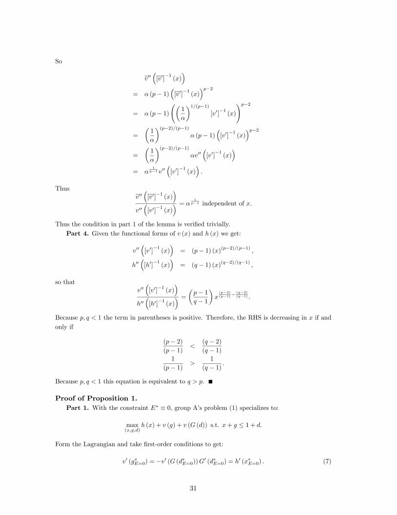
So
ev00 �[ev0]�1 (x)�= � (p� 1)
�[ev0]�1 (x)�p�2
= � (p� 1) �
1
�
�1=(p�1)[v0]
�1(x)
!p�2
=
�1
�
�(p�2)=(p�1)� (p� 1)
�[v0]
�1(x)�p�2
=
�1
�
�(p�2)=(p�1)�v00
�[v0]
�1(x)�
= �1
p�1 v00�[v0]
�1(x)�:
Thus ev00 �[ev0]�1 (x)�v00�[v0]
�1(x)� = � 1
p�1 independent of x:
Thus the condition in part 1 of the lemma is veri�ed trivially.
Part 4. Given the functional forms of v (x) and h (x) we get:
v00�[v0]
�1(x)�
= (p� 1) (x)(p�2)=(p�1) ;
h00�[h0]
�1(x)�
= (q � 1) (x)(q�2)=(q�1) ;
so thatv00�[v0]
�1(x)�
h00�[h0]
�1(x)� = �p� 1
q � 1
�x(p�2)(p�1)�
(q�2)(q�1) :
Because p; q < 1 the term in parentheses is positive. Therefore, the RHS is decreasing in x if and
only if
(p� 2)(p� 1) <
(q � 2)(q � 1)
1
(p� 1) >1
(q � 1) :
Because p; q < 1 this equation is equivalent to q > p:
Proof of Proposition 1.Part 1. With the constraint E� � 0; group A�s problem (1) specializes to:
max(x;g;d)
h (x) + v (g) + v (G (d)) s.t. x+ g � 1 + d:
Form the Lagrangian and take �rst-order conditions to get:
v0 (g�E=0) = �v0 (G (d�E=0))G0 (d�E=0) = h0 (x�E=0) : (7)
31

The proof of Lemma 1 shows thatG0 (c) 2 (�1; 0) ; hence the �rst equality in (7) implies v0 (G (d�E=0)) >v0 (g�E=0) ; which in turn implies:
G (d�E=0) < g�E=0: (8)
Now take the second equality in (7), substitute from equation (5) in the proof of Lemma 1, and
again use G0 (c) 2 (�1; 0) to write:
h0 (1� d�E=0 �G (d�E=0)) > h0 (x�E=0) ;
whence:
1� d�E=0 �G (d�E=0) < x�E=0: (9)
Adding up (8) and (9) yields:
1� d�E=0 < x�E=0 + g�E=0:
The last line can be rewritten as X (d�E=0) + G (d�E=0) < x
�E=0 + g
�E=0; which implies that more
resources are allocated to private and public good consumption in in period 1 than in period 2
(the implication follows because group 2 in period 1, as well as group 1 in period 2, are allocated
zero private consumption). So it must be d�E=0 > 0:
Part 2. In equilibrium group 1 is not allocated any private good in period 2.
Part 3. See (8).
Proof of Proposition 2.
Part 1. Let us �rst prove that d� + E� > 0: Suppose, by contradiction, that d� + E� � 0:Given that E� > 0; we have from Lemma 1 and the proof of part 3 of this Proposition, that public
good provision must be higher in period 2 than in period 1 (i.e. G (d� + E�) � g�). This impliesthat v0 (g�) > �v0 (G (d� + E�))G0 (d� + E�) : Therefore, group A could increase its lifetime payo¤by increasing public good provision in period 1. To do so, group A just has to increase debt (or
reduce surplus). So, d� + E� � 0 cannot be true. We now prove that d� + E� > d�E=0: From
Proposition 3 part 4, we know that, for E < E�; increasing E increases d�E�+ E. Thus, to get
the result, it su¢ ces to note that, in E = 0; d�E�+E = d�E=0; and that, in E = E
�, d�E�+E =
d� + E�:
Part 2. If, by contradiction, group A were to choose d� + E� = 1 then period 2�s budget
constraint implies the no public good could be provided. Because of Inada conditions for group
A�s utility function, this could never be an optimal choice for group A.
Part 3. Fix any d (for example, d = d�) and consider the vector (x; g; E) that solves problem(1) conditional on the debt level being set at d. The conditional problem is separable in the sense
that the x and g that solve the conditional problem (1) are the solutions to the following simpler
problem which does not involve E:
max(x;g)
h (x) + v (g) s.t. x+ g � 1 + d:
This problem was introduced in De�nition 1, and so the g that solves the conditional problem (1)
must be exactly G (�d) : The solution to the unconditional problem (1) is then g� = G (�d�) : Nowfrom Lemma 1 we know that G (�) is a decreasing function, so if d� is positive then g� = G (�d�) >
32

G (d� + E�) : The inequality is the desired conclusion.
Part 4. Suppose, by contradiction, that the marginal value of group A�s private consumptionwas larger in period 2. Then group A could reduce debt (or increase surplus) by one unit, and
simultaneously increase entitlements by one unit. This operation would not change group B�s
optimization problem in period 2, hence public good provision in period 2 would be unchanged;
and it would increase group A�s lifetime utility.
Part 5. See Proposition 8 part 3 in the Appendix F.
Additional Example
In the text we showed how debt and entitlements respond to changes in � for a case in
which there is relatively high con�ict between groups, i.e., � = 0:5. We now consider a
case with relatively low con�ict, i.e., � = 1:5. When �! 0, there is essentially no con�ict
between groups because group B spends the entire budget on the public good. Thus, in
this case, the optimal debt (entitlements) level goes to zero as � goes to zero. When �
increases, con�ict starts mattering, but the e¤ect di¤ers for debt and entitlements. For
debt, and the crowdout e¤ect �rst dominates so debt rises until it is overtaken by the
smoothing e¤ect and debt drops. For entitlements, both e¤ects pull in the same direction.
Because group B starts allocating resources to its private consumption, the crowdout e¤ect
pulls entitlements up. Because of the change in the concavity of the utility function, group
A wants to balance private and public consumption more in period 2. Given that we start
from zero private consumption (and full public consumption), this requires an increase in
entitlements.
0.5 1.0 1.5 2.0
0.2
0.0
0.2
0.4
0.6
rho
Entitlements (Green); Debt with entitlement (Plain Blue); Debt without entitlements (Dashed
Blue).
Appendix B: Proofs of Section 5
Proof of Proposition 3.
33

Part 1. Fix any d and consider the vector (x; g; E) that solves problem (1) conditional on the
debt level being set at d. The entitlement level that solves the conditional problem is the solution
to the following simpler problem which does not involve x or g:
maxEh (E) + v (G (d+ E)) : (10)
The �rst order conditions read:
h0 (E) = �v0 (G (d+ E))G0 (d+ E) : (11)
The LHS is an decreasing function of E: Because v (G (d+ E)) is concave in E, its �rst derivative
with respect to E; v0 (G (�))G0 (�) ; is a decreasing function of E: The RHS is its opposite, andtherefore an increasing function of E. Now increase d: The LHS function stays unchanged. The
RHS function shifts up. Therefore the two functions now cross at a lower level of E:
Part 2. Fix any E and consider the vector (x; g; d) that solves problem (1) conditional on the
entitlement level being set at E. The debt level that solves the conditional problem is the solution
to the following simpler problem:
max(x;g;d)
h (x) + v (g) + v (G (d+ E)) s.t. x+ g � 1 + d:
De�ne the following value function:
U (d) = max(x;g)
h (x) + v (g) s.t. x+ g � 1 � d: (12)
Because h (�) and v (�) are concave, U (d) is concave in d: Our problem can then be rewritten as
follows:
maxdU (d) + v (G (d+ E)) . (13)
This problem is isomorphic to (10), and the rest of the proof follows the argument in part 1.
Part 3. Consider any �d < d: Suppose by contradiction that
�d +E
� �d�> d+E
�d�: Then,
because the RHS of (11) is an increasing function of d+ E; we have:
�v0�G� �d + E
� �d���
G0� �d + E
� �d��> �v0
�G�d+ E
�d���
G0�d+ E
�d��: (14)
Now, we know from part part 1 that E� �d�> E
�d�: Because h0 (�) is a decreasing function it
follows that:
h0�E� �d��< h0
�E�d��: (15)
By de�nition of E�d�; the RHS of (14) must equal the RHS of (15). But then it follows that:
h0�E� �d��< �v0
�G� �d + E
� �d���
G0� �d + E
� �d��;
which contradicts the de�nition of E� �d�:
Part 4. Problem (13) is isomorphic to (10), and the rest of the proof follows the argument in
part 3.
34

Appendix C: Proofs of Section 6
Proof of Proposition 4. The proof starts with a foundational result. Let g�(d) and E�d�
denote the optimal choice of period-1 public good and entitlements, respectively, conditional on a
debt level d. Suppose a debt ceiling d is binding for group A. We now show that relaxing the debt
ceiling increases group B�s lifetime utility if
�G0�d+ E(d)
� @g� �d�@d
> 1 + E0�d�:
Let x�(d) and g��d�denote the optimal choice of private and public goods, respectively, in the
�rst period conditional on a debt level d. Similarly, X(d + E) and G�d+ E
�denote the optimal
choice of private and public goods, respectively, by group B in the second period conditional on a
debt level d and an entitlements level E:
(i) Period-1 social return to relaxing debt limit.
Suppose a binding debt cap is increased by one dollar (so the budget available to group A
increases). The variation in period-1 utility for group A is:
@W 1A
@d= v0
�g��d��:
The variation in period-1 utility for group B is:
@W 1B
@d= v0
�g��d�� @g� �d�
@d
(ii) Period-2 social return to relaxing debt limit.
Let E�d�denote the solution to problem (10) for d = d: The period-2 total variation in utility
for group A is given by
@W 2A
@d= E0(d)h0
�E(d)
�+�1 + E0
�d��G0�d+ E(d)
�v0�G�d+ E(d)
��:
Use the �rst-order conditions (11) to simplify this expression:
@W 2A
@d= G0
�d+ E(d)
�v0�G�d+ E(d)
��:
The total variation in utility for group B is given by
@W 2B
@d=�1 + E0
�d�� �X 0(d+ E(d))h0
�X(d+ E(d))
�+G0
�d+ E(d)
�v0�G�d+ E(d)
���:
The �rst order conditions for group B require that h0�X(d)
�= v0
�G�d+ E(d)
��; whence
@W 2B
@d=�1 + E0
�d����X 0(d+ E(d)) +G0
�d+ E(d)
��� v0�G�d+ E(d)
��:
From the proof of Lemma 1 we have that X 0(�) + G0 (�) = �1: Substitute into group B�s total
35

variation to get:@W 2
B
@d= �
�1 + E0
�d��� v0�G�d+ E(d)
��:
(iii) Conditions for improvement in group B�s lifetime utility:
By assumption the debt limit is binding for group A, which implies:
@W 1A
@d+@W 2
A
@d= v0
�g��d��+ v0
�G�d+ E(d)
��G0�d+ E(d)
�> 0: (16)
Group B�s lifetime utility is given by:
@W 1B
@d+@W 2
B
@d= v0
�g��d�� @g� �d�
@d� v0
�G�d+ E(d)
�� �1 + E0
�d��
> v0�G�d+ E(d)
�� "�G0
�d+ E(d)
� @g� �d�@d
��1 + E0
�d��#
; (17)
where the inequality follows from (16). This expression has the same sign as the expression in
brackets. The desired statement follows (remember that we now work under the assumption that
h (x) = v (x) have a CRRA form (x)1��
= (1� �)):Part 1. If debt is unconstrained, that is, d = d�; then the inequality in (16) is replaced by
an equality. Consequently, the inequality in (17) is replaced by an equality. Thus the variation
in group B�s lifetime utility from forcing group A to incur slightly more debt than they would
choose to is exactly equal to the RHS of (17). If � > (log 2= log 6) ; Proposition 11 part 3 ensures
that the bracketed term in expression (17) is negative for any d. Hence group B su¤ers from
relaxing the binding constraint. Group A is indi¤erent at the margin because we assumed that the
constraint was barely binding. Conversely, therefore, tightening any barely-binding constraint on
debt makes group A no worse o¤ and group B strictly better o¤ at the margin. The case where
� < (log 2= log 6) is exactly symmetric.
Part 2. If debt is constrained at d < d�; then the variation in group B�s lifetime utility
from allowing group A to incur slightly more debt is bounded below by the RHS of (17). Since
� < (log 2= log 6) ; Proposition 11 part 3 ensures that the bracketed term in expression (17) is
positive for any d. Hence group B bene�ts from relaxing the binding constraint. Group A bene�ts
too because we assumed that the constraint was binding. Conversely, therefore, tightening any
binding constraint on debt strictly hurts both groups.
Proof of Proposition 5.Part 1. Group A�s allocation problem can be described as a constrained optimization problem.
If a constraint on entitlements barely binds, its Lagrange multiplier will be close to zero. In the
limit, it will be exactly zero. Thus the marginal impact on group A�s lifetime payo¤ of introducing
a constraint on entitlements is zero. Let�s now consider the e¤ects on group B�s lifetime payo¤.
Proposition 3 part 4 ensures that tightening a cap on entitlements reduces the total obligations
that group A bequeaths to group B. This means that group B is strictly better o¤ in period 2.
Also, group B is strictly better o¤ in period 1 because constraining entitlements leads group A to
increase debt (Proposition 3 part 2), and part of the additional period-1 resources will be allocated
to the public good in period 1, from which group B bene�ts.
36

Part 2. Follows from the Inada condition on group A�s utility for the private good.
Appendix D: Proofs of Section 7
The next proof makes use of the following property:
Lemma 3 Let f(x; y) be a concave function. Denote y� (x) = argmaxx f(x; y) and
F (x) = f (x; y� (x)) : Then F (x) is concave.
Proof. The �rst derivative of F is:
@
@xF (x) = fx + fy � y�0 (x) :
The second derivative of F is:
@2
@x2F (x) = fxx + fxy � y�0 (x) + [fyx + fyy � y�0 (x)] y�0 (x) + fy � y�00 (x)
=h1 y�0 (x)
i "fxx fxy
fyx fyy
#"1
y�0 (x)
#+ fy � y�00 (x) :
The last addend is zero because fy = 0 by de�nition of y� (x) : So the above is a quadratic form of
the Hessian, and the quadratic form is negative by concavity of f(x; y). Hence @2
@x2F (x) < 0:
Proof of Proposition 6.Part 1. Substitute E (d) � 0 into equation (19) below and repeat the argument that follows.
Proposition 1 part 1 ensures that at � = 0 we have d� > 0. The desired conclusion then follows
from part 4.
Part 2. If group A persists in power it faces the following period-2 allocation problem:
maxx;g
h (x) + v (g) s.t. x+ g � 1� d:
The solution to this problem is given by X (d), G (d) (refer to Lemma 1). Using these expressions
we can write group A�s allocation problem as follows:
1.
maxd;E
U (d) + � [h (1� d�G (d)) + v (G (d))] + (1� �) [h (E) + v (G (d+ E))] ; (18)
where U (d) is de�ned in (12). Fix d; due to multiplicative separability of E and �, the
optimal level of entitlements E (d) is independent of �: This means that any e¤ect of varying
� on E�; the equilibrium level of entitlements, must be channeled through the choice of debt,
that is:@E�
@�=@E (d)
@d
@d�
@�:
Because E (d) is independent of �; Proposition 3 part 1 applies, ensuring that @E (d) =@d < 0:
Thus we have proved that equilibrium debt and entitlement move in opposite directions when
� varies.
37

Part 3. It follows directly from the previous step that
@d�
@�+@E�
@�=@d�
@�
�1 +
@E (d)
@d
�:
It thus remains to prove that 1 + @E(d)@d > 0: Di¤erentiating equation (3) implicitly, we obtain:
@E
@d= � v00 (GB (d+ E)) (G
0B (d+ E))
2+ v0 (GB (d+ E))G
00B (d+ E)
h00 (E) + v00 (GB (d+ E)) (G0B (d+ E))2+ v0 (GB (d+ E))G00B (d+ E)
From the concavity of v (GB (�)) and the concavity of h (�), we have that this is larger than �1:Part 4. We �rst need to prove that the objective function in equation (18) is concave. Rewrite
this by distributing U (d) in the two brackets. This yields
� [h (1 + d� g� (d)) + v (g� (d)) + h (1� d�G (d)) + v (G (d))] + (19)
(1� �) [h (1 + d� g� (d)) + v (g� (d)) + h (E (d)) + v (G (d+ E (d)))] :
We prove that the functions in the two brackets are concave in d. Taking the second derivative of
the �rst bracket gives:
�[h00 (1 + d� g (d)) (1� g0 (d))2 � h0 (1 + d� g (d)) g00 (d) + v00 (g (d)) (g0 (d))2 + v0 (g (d)) g00 (d) +h00 (1� d�G (d)) (1 +G0 (d))2 � h0 (1� d�G (d))G00 (d) + v00 (G (d)) (G0 (d))2 + v0 (G (d))G00 (d)]
By de�nition of g� (d) we have h0 (1 + d� g� (d)) = v0 (g� (d)) ; and by de�nition of G (d) ; we haveh0 (1� d�G (d)) = v0 (G (d)) : Therefore, the expression boils down to
�[h00 (1 + d� g (d)) (1� g0 (d))2+v00 (g (d)) (g0 (d))2+h00 (1� d�G (d)) (1+G0 (d))2+v00 (G (d)) (G0 (d))2]
From the concavity of h (�) ; v (�) ; and v (G (�)) ; we have that this is necessarily negative. For thefunction in the second bracket, �rst note that the following function is concave in (d;E):
h (1 + d� g� (d)) + v (g� (d)) + h (E) + v (G (d+ E)) :
We know from the proof of Proposition 3 that h (1 + d� g� (d)) + v (g� (d)) is concave in d andthus (d;E). Furthermore, we have that (i) h (E) is a concave function of (d;E) (by assumption),
and (ii) because d + E is a concave function of (d;E), and v (G (�)) is concave (by assumption),then v (G (d+ E)) is also concave in (d;E). Given that E (d) solves problem 10, we can apply
Lemma 3, to show that the function in the second bracket is concave in d:
We can now prove that d� (�) ; the value of d that maximizes 19 for a given �, is monotonic in
�: By the concavity of the functions in the two brackets of 19, we have that
@
@d[h (1 + d� g� (d)) + v (g� (d)) + h (1� d�G (d)) + v (G (d))] , and
@
@d[h (1 + d� g� (d)) + v (g� (d)) + h (E (d)) + v (G (d+ E (d)))]
are both decreasing functions. Denoting by d1 and d2; respectively, the values at which these two
functions are equal to 0; we have that d� (�) lies in the interval with extremes d1 and d2, where d1
38

may be larger or smaller than d2. In that interval, one of the two functions must be negative, and
the other one positive. Thus, increasing � moves d� (�) monotonically towards d1. To conclude
the proof, note that we have d� (1) = 0 (when A is the social planner, smoothing requires no debt
or surplus); thus if debt started out positive at � = 0 then it must monotonically decrease with
�; and if debt started out negative at � = 0 then it must monotonically increase in �: Together
with part 2 of this Proposition, this shows that entitlements are monotonic in � (in the opposite
direction as debt).
Appendix E: Proofs of Section 8
Proof of Proposition 7. From Proposition 10 in Appendix F. we have that: E� is decreasing
in � for any � > 0; for � < 1; d� is decreasing in � if and only if � is smaller than
24 ��
1���1��
�1��
�35�;
for � > 1; d� is decreasing in � if and only if � is greater than
24 ��
1���1��
�1��
�35� :
Appendix F: CRRA Preferences
In this Appendix we provide closed-form solutions for the equilibrium under the assump-
tion that groups have CRRA preferences, that is, when:
ui�xti; x
tj ; g
t�=
�xti�1��i
1� �i+ �i
�gt�1��i
1� �i;
with �i > 0:
Note that we allow the possibility that �A 6= �B and �A 6= �B. This type of hetero-geneity is not contemplated in the main model, but this extension poses no di¢ culties. To
simplify notation, �A = � and �A = �:
Period 2
Group B�s problem is
maxg
(1� d� E � g)1��B1� �B
+ �Bg1��B
1� �B:
The �rst order with respect to g read:
(1� d� E � g)��B = �Bg��B ;
and solving for g yields the public good allocation in period 2:
39

G (d+ E) =�
1�BB
1 + �1�BB
(1� d� E) : (20)
Group B�s private consumption in period 2, X (d+ E) ; can be recovered from the budget
constraint G (d+ E) +X (d+ E) = 1� d� E.
Note that this implies v (G (d+ E)) =
0B@ �
1�BB
1+�
1�BB
(1�d�E)
1CA1��B
1��B.
Period 1
Group A�s problem is:
maxg;E;d
(1 + d� g)1��
1� � + �g1��
1� � +E1��
1� � + �
�
1�BB
1+�1�BB
(1� d� E)!1��
1� � :
Let g�(d) and E�d�denote the optimal choice of period-1 public good and entitlements,
respectively, conditional on a debt level d.
Lemma 4 (period-1 equilibrium allocations conditional on a given debt level inthe CRRA case)
1. The equilibrium allocation of period-1 public good conditional on a debt level d, is
g�(d) =�1 + d
��1�
1+�1�;
2. The equilibrium allocation of entitlements conditional on a debt level d, is E(d) =
�1� d
�=
2641 + � 1�
0@ �1�BB
1+�
1�BB
1A1���
375 :Proof.
Part 1. The function g�(d) solves the following problem:
g�(d) = argmaxg
�1 + d� g
�1��1� � + �
g1��
1� � :
The �rst order with respect to g reads:�1 + d� g
���B = �g��;and solving for g yields:
g�(d) =�
1�
1 + �1�
�1 + d
�
40

Part 2. The function E(d) solves the following problem:
E(d) = argmaxE
E1��
1� � + �
0@ �1
�B
B
1 + �1�B
B
1A1�� �1� d� E
�1��1� � :
The �rst order with respect to E read:
�
0@ �1
�B
B
1 + �1�B
B
1A1�� �1� d� E
���= E��;
and solving for E yields, after some algebra:
E(d) =1
1 + �1�
�
1�BB
1+�
1�BB
! 1���
�1� d
�: (21)
Lemma 5 The equilibrium level of debt in the CRRA case is determined by the following
condition:
(1� d)(1 + d)
=
0BB@1 + � 1�
0B@ �1�BB
1 + �
1
�BB
1CA1���
1CCA 1�1 + �
1�
� : (22)
Proof. Substitute the expressions for g�(d) and E(d) into group A�s period-1 problem:
maxd
(1 + d�K (1 + d))1��
1� � + �(K (1 + d))
1��
1� � +(Z (1� d))1��
1� � + �
�
1�BB
1+�1�BB
(1� d� Z (1� d))!1��
1� �
= maxd
(1 + d)1��
1� �
h(1�K)1�� + �K1��
i+(1� d)1��
1� �
264Z1�� + �0@ �
1�B
B
1 + �1�B
B
(1� Z)
1A1��375 ; (23)
where we have denoted K = �1�
1+�1�and Z = 1=
24� 1�
�
1�BB
1+�
1�BB
! 1���
+ 1
35 : The problem is concave
in d: The �rst order conditions with respect to d are:
(1 + d)��h(1�K)1�� + �K1��
i= (1� d)��
264Z1�� + �0@ �
1�B
B
1 + �1�B
B
(1� Z)
1A1��375 ;
41

or equivalently:
(1� d)(1 + d)
=
8><>:264Z1�� + �
0@ �1�B
B
1 + �1�B
B
(1� Z)
1A1��375" 1
(1�K)1�� + �K1��
#9>=>;1=�
:
After much algebra, the �rst term in square brackets simpli�es to:0B@� 1�
0@ �1�B
B
1 + �1
�B
B
1A1���
+ 1
1CA�
;
and the second term in square brackets simpli�es to:�1 + �
1�
���:
Substituting back into the �rst order conditions we get equation (22).
Proposition 8 (properties of the equilibrium in the CRRA case). In the CRRAcase (with the same �):
1. the equilibrium level of debt is strictly interior: d� 2 (�1; 1) ;
2. d� = 0 when � = 1;
3. d� > 0 if and only if � < 1;
4. the equilibrium level of entitlements is strictly positive, E� > 0;
5. in equilibrium, total obligations, that is, debt and entitlements, are related by the
following proportion: (1 + d�) =E� =�1 + �
1�
�:
Proof.Part 1. The RHS of (22) is nonnegative. The LHS of (22) goes from +1 at d = �1 to 0
at d = 1; and it is a decreasing function of d on [�1; 1] : Therefore, the equilibrium level of debt
d� 2 (�1; 1) :Part 2. The RHS of (22) equals 1 when � = 1; hence d� = 0 when � = 1:Part 3. d� > 0 if and only if the RHS of (22) is smaller than 1, that is, if and only if:
0@ �1�B
B
1 + �1
�B
B
1A1���
< 1;
which is the case if and only if 1� � > 0 or � < 1:Part 4. E� = E (d�) : The conclusion follows from expression (21) and the fact that d� < 1:
42

Part 5. Combine expressions (21) and (22) to get:
E(d�) =1
1 + �1�
�
1�BB
1+�
1�BB
! 1���
(1� d�)
=1 + d��1 + �
1�
� :
Proposition 9 In the CRRA case (with the same �) we have: d� = 1�h(z)1+h(z) and E
� =
2[1+h(z)](1+z) where z = �
1� and h (z) = 1
(1+z) +�
z1+z
� 1�:
Proof. From Lemma 5, we know that
(1� d)(1 + d)
=
0@1 + � 1�
�
1�
1 + �1
�
! 1���
1A 1�1 + �
1�
� :Make the change of variable: �
1� = z > 0: Because � > 0 by assumption, z is a monotonic function
of �: Then
(1� d)(1 + d)
=
1 + z
�z
1 + z
� 1���
!1
(1 + z)
=1
(1 + z)+
�z
1 + z
� 1�
:
Denote:
h (z) =1
(1 + z)+
�z
1 + z
� 1�
:
Then we have:
(1� d)(1 + d)
= h (z) ; (24)
d� =1� h (z)1 + h (z)
:
Take the expression for E (d) from Lemma 4, and substitute z to get:
E(d) =(1� d)
(1 + z)h (z):
Substitute from (24) to get:
E� =2
[1 + h (z)] (1 + z)
43

Proposition 10 (comparative statics with respect to �) In the CRRA case (with
the same �) :
1. E� is decreasing in � for any � > 0.
2. d� is decreasing in �: for 0 < � < 1 if and only if � is larger than
24 ��
1���1��
�1��
�35� ;
for � > 1 if and only if � is smaller than
24 ��
1���1��
�1��
�35�.
Proof.Part 1. E� is increasing in z if and only if [1 + h (z)] (1 + z) is decreasing in z: First, compute:
h (z) =1
(1 + z)+
�z
1 + z
� 1�
:
h0 (z) = � 1
(1 + z)2 +
1
�
�z
1 + z
� 1��1 1
(1 + z)2 :
Then
@
@z[1 + h (z)] (1 + z)
= h0 (z) (1 + z) + 1 + h (z)
=
"� 1
(1 + z)2 +
1
�
�z
1 + z
� 1��1 1
(1 + z)2
#(1 + z) + 1 +
1
(1 + z)+
�z
1 + z
� 1�
=1
�
�z
1 + z
� 1��1 1
(1 + z)+ 1 +
�z
1 + z
� 1�
> 0:
Hence E� is decreasing in z; and hence in �; for any � > 0:
Part 2. We have:
d� =1� h (z)1 + h (z)
@
@zd� =
�h0 (z) (1 + h (z))� (1� h (z))h0 (z)(1 + h (z))
2
This has the same sign as its numerator:
�h0 (z) (1 + h (z))� (1� h (z))h0 (z)= �2h0 (z)
= 21
(1 + z)2
"1� 1
�
�z
1 + z
� 1��1#:
This expression is positive i¤
� >
�z
1 + z
� 1���
:
44

So debt is increasing in z if and only if � >�
z1+z
� 1���
: In the case 0 < � < 1; this condition
rewrites as:
0 < � <
��1=�
1 + �1=�
� 1���
���
1���1=� < ��
1�� < �1=� � ��
1���1=�
�
24 ��
1���1� �
�1��
�35� � <
24 ��
1���1� �
�1��
�35� < �
So if 0 < � < 1 then debt is decreasing in � for � larger than
24 ��
1���1��
�1��
�35�. In the case 1 < �;
the condition rewrites as:
0 < � <
��1=�
1 + �1=�
� 1���
1 > ��
1��
�1 + �1=�
�> �1=�
1 >
24 ��
1���1� �
�1��
�35� > �
So if 1 < � then debt is decreasing in � for � smaller than
24 ��
1���1��
�1��
�35�.
Proposition 11 (welfare properties of a constrained equilibrium in the CRRAcase). In the CRRA case with �B = � and �B = �:
1. a zero-debt cap is binding if and only if � < 1;
2. relaxing a binding zero-debt cap is Pareto-optimal if:
��1�
� 2��1�
�1 + �
1
�
� 1���
+��1�
� �+1�>
�1 + �
1
�
�2;
3. if � = 1 then relaxing a zero-debt cap is Pareto-optimal if � < log 2= log 6 ' 0:39:
4. if � = 1� " then relaxing a binding zero-debt cap is never Pareto-optimal for any �provided that " is su¢ ciently small.
Proof.Part 1. Expression (23) describes group A�s period-1 allocation problem as a function of d alone.
In the case � < 1 the unconstrained optimum d� exceeds 0 (see Proposition 8 part 3). A zero-debt
cap rule out d�: Because problem (23) is concave in d; the constrained optimum is for group A to
45

choose debt right up to the ceiling. Thus a zero-debt cap is binding. If � > 1 Proposition 8 part 3
indicates that a zero-debt cap is not binding.
Part 2. In the CRRA case, we can leverage (20) and Lemma (4) to write:
�G0�d+ E(d)
�=
�1�B
B
1 + �1�B
B
;
@g��d�
@d=
�1�
1 + �1�
;
E0�d�= � 1
1 + �1�
�
1�BB
1+�
1�BB
! 1���
:
Recall the condition Proposition 4 states that if a debt ceiling d is binding for group A, then
relaxing the debt ceiling increases group B�s lifetime utility if
�G0�d+ E(d)
� @g� �d�@d
> 1 + E0�d�:
Substitute to get:
�1�B
B
1 + �1�B
B
�1�
1 + �1�
> 1� 1
1 + �1�
�
1�BB
1+�
1�BB
! 1���
Set �B = � and �B = �; then manipulate the previous equation to get:��
1�
� 2��1��1 + �
1
�
� 1���
+��
1�
�2>�1 + �
1
�
�2: (25)
Part 3. When � = 1 condition (25) specializes to:
21��� + 1 > 4:
After some manipulation, this condition is seen to be equivalent to:
� <log 2
log 6:
Part 4. When � = 1 condition (25) specializes to:
�+ �2 > (1 + �)2:
This condition never holds for any � > 0: Therefore, if � = 1� " condition (25) must also fail for" small enough.
46
References
[1] Aaron, H. (2007) �Budget Crisis, Entitlement Crisis, Health Care Financ-
ing Problem�Which Is It?� Health A¤airs, 26, no.6:1622-1633. Available at
http://content.healtha¤airs.org/content/26/6/1622.full.html
[2] Alesina, A. and R. Perotti (2000). �Budget De�cits and Budget Institutions,�in J. Poterba,
ed., Fiscal Institutions and Fiscal Performance, Chicago: University of Chicago Press.
[3] Alesina, A. and G. Tabellini (1990) �A Positive Theory of Fiscal De�cits and Government
Debt.�Review of Economic Studies (1990) 57 (3): 403-414.
[4] Arpaia, A., K. Dybczak, and F. Pierini (2009). �Assessing the short-term impact of pension
reforms on older workers�participation rates in the EU: a di¤-in-di¤ approach.�European
Commission, Economic Papers 385, September 2009.
[5] Aubuchon, C., J. Conesa, and C. Garriga (2011). �A Primer on Social Security Systems and
Reforms.�Federal Reserve Bank of St. Louis Review, 93(1), pp. 19-35.
[6] Azariadis, C. and V. Galasso (2002). �Fiscal Constitutions.� Journal of Economic Theory,
103(2), pp. 255-281.
[7] Azzimonti, M. (2015), �Partisan Con�ict and Private Investment,� NBER working paper,
21273.
[8] Azzimonti, M., M. Battaglini, and S. Coate (2015). �The Costs and Bene�ts of Balanced
Budget Rules: Lessons from a Political Economy Model of Fiscal Policy.�Journal of Public
Economics, forthcoming.
[9] Azzimonti, M., E. de Francisco, and V. Quadrini (2014). "Financial Globalization, Inequality,
and the Rising Public Debt." American Economic Review, 104(8): 2267-2302.
[10] Badinger, H. andW. Reuter (2015). �The Case for Fiscal Rules,�University of Vienna working
paper.
[11] Battaglini, M. (2011), �The Political Economy of Public Debt,�Annual Review of Economics,
3, 161-189.
[12] Battaglini, M. and S. Coate (2008), �A dynamic theory of public spending, taxation, and
debt,�American Economic Review, Vol. 98, No. 1, 201-236.
[13] Boadway, R. and Wildasin, D. (1989) �A Median Voter Model of Social Security,� Interna-
tional Economic Review, Vol. 30, pp. 307-328.
[14] Bonoli, G. (2000). The politics of pension reform: institutions and policy change in Western
Europe. Cambridge University Press.
47

[15] Bowen, R., Y. Chen, and H. Eraslan (2014) �Mandatory Versus Discretionary Spending: the
Status Quo E¤ect,�American Economic Review, 104(10): 2941-2974
[16] Bowen, R., Y. Chen, H. Eraslan, and J. Zapal (2015) �E¢ ciency of Flexible Budgetary
Institutions,�working paper.
[17] Browning, E. (1975), �Why the Social Insurance Budget is too Large in a Democracy;�
Economic Inquiry, Vol. 22, pp. 373-388.
[18] Conde-Ruiz, J. I. and V. Galasso (2005), �Positive Arithmetic of Social Security.�Journal of
Public Economics; vol. 89, pp. 933-955.
[19] Conesa, J. and C. Garriga (2008). �Optimal Fiscal Policy in the Design of Social Security
Reforms.�International Economic Review, 49(1), pp. 291-318.
[20] Crain, M. and Tollison R.(1993) �Time Inconsistency and Fiscal Policy: Empirical Analysis
of US States, 1969-89.�Journal of Public Economics, Vol. 51, pp. 153-159.
[21] Cukierman, A. and A. Meltzer, (1989), �A Political Theory of Government Debt and De�cits
in a Neo-Ricardian Framework,�American Economic Review, Vol. 79, No. 4, Pages 713-732.
[22] Davey, M. (2015) �Illinois Supreme Court Rejects Lawmakers�Pension Overhaul,�New York
Times, May 8, 2015. Available at http://www.nytimes.com/2015/05/09/us/illinois-supreme-
court-rejects-lawmakers-pension-overhaul.html?
[23] Eberstadt, N. (2016). America�s Entitlements Explosition. Statement before the House Com-
mittee on the Judiciary.
[24] Evans, R., L. Kotliko¤, and K. Phillips (2012), �Game Over: Simulating Unsustainable Fiscal
Policy,�NBER working paper, 17917.
[25] European Commission (2012). Fiscal Sustainability Report.
[26] Franzese, R. (2002). �The Positive Political Economy of Public Debt: An Empirical Exami-
nation of the OECD Postwar Experience through the 1990s,�University of Michigan working
paper.
[27] Fox, B. (2014). �Portuguese court throws out �unconstitutional�pay and pension cuts.�Pub-
lished on euobserver, 2. JUN 2014, https://euobserver.com/news/124434
[28] Galasso, V. (2008). The Political Future of Social Security in Aging Societies. Cambridge:
MIT Press,
[29] Galasso, V. and P. Profeta (2004). �Lessons for an Ageing Society: The Political Sustainability
of Social Security Systems.�Economic Policy, pp. 63-115.
48

[30] Gingrich, J. (2015). �Still Not Dismantling? The Legacy of Dismantling the Wel-
fare State in Comparative Politics.� PS: Political Science & Politics, 48, pp. 279-283.
doi:10.1017/S1049096514002194.
[31] Golosov, M., A. Tsyvinski, and I. Werning (2006) �New Dynamic Public Finance: A User�s
Guide�in NBER Macroeconomics Annual Volume 21, edited by Acemoglu, D., K. Rogo¤ and
M. Woodford.
[32] Grossman, G. and E. Helpman (1998). �Intergenerational Redistribution with Short-Lived
Governments.�Economic Journal, 108, pp. 1299-1329.
[33] Hallerberg, M. and J. Von Hagen (2000) �Electoral Institutions, Cabinet Negotiations, and
Budget De�cits in the European Union�in Fiscal Institutions and Fiscal Performance, edited
by Poterba, J. and J. Von Hagen. University of Chicago Press.
[34] Hansson , L. and C. Stuart (1989). �Social Security as Trade among Living Generations.�
American Economic Review, 79, pp. 549-559.
[35] Hou, Y. and D. Smith (2006). �A Framework for Understanding State Balanced Budget Re-
quirement Systems: Reexamining Distinctive Features and an Operational De�nition,�Public
Budgeting and Finance, Fall, pp. 22-45
[36] Kalandrakis, T. (2004), �A Three-Player Dynamic Majoritarian Bargaining Game,�Journal
of Economic Theory, 116: 294-322.
[37] Kotliko¤, L. and S. Burns (2004) The Coming Generational Storm MIT Press.
[38] Lambertini, L. (2003) �Are Budget De�cits Used Strategically,�SSRN working paper.
[39] Lanza, E. M., and T. J. Nicola (2014). �Social Security reform: Legal analysis of Social
Security bene�t entitlement issues.�Washington, DC: Congressional Research Service.
[40] Lizzeri, A. (1999), �Budget De�cits and Redistributive Politics,�Review of Economic Studies,
Vol. 4, Pages 909-928.
[41] McCarty, N., K. Poole, H. Rosenthal (2006), Polarized America: The Dance of Ideology and
Unequal Riches, MIT Press.
[42] Merler, S. (2015) � �Dura Lex, sed Lex�(?)�Published May 22, 2015. Available on Bruegel
at http://bruegel.org/2015/05/dura-lex-sed-lex/
[43] Mesa-Lago, C. and G. Márquez (2007). �Reform of Pension and Social Assistance Systems.�
In The State of State Reform in Latin America edited by Eduardo Lora, Stanford University
Press 1450 Page Mill Road Palo Alto, CA 94304.
49

[44] Monahan, A. (2013). �Understanding the Legal Limits on
Public Pension Reform.� AEI Working Paper, available at
http://www.nasra.org/Files/Topical%20Reports/Legal/Monahan1305.pdf
[45] Mulligan, C. and X. Sala-i-Martin (1999). �Gerontocracy, Retirement and Social Security.�
NBER Working Paper, 7117.
[46] Munnell, A. and L. Quinby (2012). �Legal Constraints on Changes in State and Local Pen-
sions.� Center for Retirement Research at Boston College, State and Local Pension Plans
Number 25, August 2012.
[47] Myles, J., and J. Quadagno. 2002. �Political Theories of the Welfare State�. Social Service
Review 76 (1). University of Chicago Press: 34�57. doi:10.1086/324607.
[48] OECD (2012), �Social spending during the crisis: So-
cial expenditure (SOCX) data update 2012.� Available at
http://www.oecd.org/els/soc/OECD2012SocialSpendingDuringTheCrisis8pages.pdf
[49] OECD (2013), �Recent pension reforms and their distributional impact�, in
Pensions at a Glance 2013: OECD and G20 Indicators, OECD Publishing.
http://dx.doi.org/10.1787/pension_glance-2013-4-en
[50] OECD (2014). �Social Expenditure Update - Social spending is falling in some
countries, but in many others it remains at historically high levels.� Available at
http://www.oecd.org/els/soc/OECD2014-Social-Expenditure-Update-Nov2014-8pages.pdf
[51] Orenstein, M. (2000). �How Politics and Institutions A¤ect Pension Reform in Three Post-
communist Countries.�Policy Research Working Paper No. 2310. World Bank, Washington,
DC.
[52] Ozler, S. and G. Tabellini (1991) �External Debt and Political Instability,�NBER working
paper.
[53] Persson, T. and L. Svenson (1989), �Why a Stubborn Conservative Would Run a De�cit:
Policy with Time Inconsistent Preferences,�Quarterly Journal of Economics, Vol. 104, No.
2, Pages 325-345.
[54] Pierson, Paul (1994) Dismantling the Welfare State? Reagan, Thatcher, and the Politics of
Retrenchment Cambridge, England: Cambridge University Press.
[55] Poterba, J. (1996). �Budget Institutions and Fiscal Policy in the U.S. States,� American
Economic Review, 86(2), Papers and Proceedings, pp. 395-400
[56] Samuelson, P. (1958). �An Exact Consumption-Loan Model of Interest With or Without the
Social Contrivance of Money,�Journal of Political Economy, 66(6), pp. 467-482.
50

[57] Schick, A. (2009). �Budgeting for Entitlements,�OECD Journal on Budgeting, 2009/2, pp.
1-13.
[58] Schaechter, A., Kinda, T., Budina, N. and A. Weber (2012). �Fiscal Rules in Response to the
Crisis �Toward the �Next-Generation�Rules. A New Dataset.�IMF WP/12/187.
[59] Social Protection - Human Rights (2009) �Protecting pensions against austerity measures in
Latvia.�Available at http://socialprotection-humanrights.org/legaldep/protecting-pensions-
against-austerity-measures-in-latvia.
[60] Song, Z., K. Storesletten, and F. Zilibotti (2014), �Rotten Parents and Disciplined Children:
A Politico-Economic Theory of Public Expenditure and Debt,� Econometrica, 80(6), pp.
2785-2803.
[61] Stantcheva, S. (2014) �Optimal Income Taxation with Adverse Selection in the Labour Mar-
ket.�Review of Economic Studies, Vol. 81, pp. 1296-1329.
[62] Stantcheva, S. (2016) �Optimal Taxation and Human Capital Policies over the Life Cycle.�
Journal of Political Economy, forthcoming.
[63] Steuerle, E. (2014) �Dead Men Ruling: How to Restore Fiscal Freedom and Rescue our
Future.�The Century Foundation Press.
[64] Stewart, N. (2008) �Turkey reforms should remain "priority".� Published 21 July 2008
on Investment and Pensions in Europe, http://www.ipe.com/turkey-reforms-should-remain-
priority/28605.fullarticle.
[65] Tabellini, G. (1991), �The Politics of Intergenerational Redistribution,�Journal of Political
Economy, Vol. 99, No. 2, Pages 335-357.
[66] Tabellini, G. and A. Alesina (1990), �Voting on the Budget De�cit,�American Economic
Review Vol. 80, No. 1, Pages 37-49.
[67] Vanhuysse, P. (2006). Divide and Pacify: Strategic Social Policies and Political Protests in
Post-Communist Democracies. Budapest: Central European University Press, Project MUSE.
Web. 29 Feb. 2016. <https://muse.jhu.edu/>.
[68] Vanhuysse, P. (2012) �Does Population Aging Drive Up Pro-Elderly Social Spending?�(Feb
2012). European Social Observatory (OSE) Research Paper Series, No. 7, 9 pages, 2012.
Available at http://ssrn.com/abstract=2404281.
[69] Velasco, A. (1996), �A Model of Endogenous Fiscal De�cits and Delayed Fiscal Reform,�
NYU working paper.
[70] Weil, P. (2008). �Overlapping Generations: The First Jubilee.� Journal of Economic Per-
spectives, 22(4), pp. 115-134.
51