the political economy of infrastructure …556.pdf · the political economy of infrastructure...

THE POLITICAL ECONOMY OF INFRASTRUCTURE INVESTMENT: COMPETITION, COLLUSION AND

UNCERTAINTY By

Arghya Ghosh and Kieron Meagher

ANU Working Papers in Economics and Econometrics # 556

October, 2011

JEL: D43, L13, H4

ISBN: 086831 556 7

THE POLITICAL ECONOMY OF INFRASTRUCTURE INVESTMENT:COMPETITION, COLLUSION AND UNCERTAINTY

ARGHYA GHOSH AND KIERON MEAGHER

ABSTRACT. Infrastructure, as it impacts transport costs, is crucial in determiningequilibrium outcomes in spatial competition; however, infrastructure investment istypically exogenous. Our political economy analysis of infrastructure choice is basedupon consumer preferences derived from Salop’s circular city model. In this setting,infrastructure investment has two effects: it directly lowers costs to consumers andindirectly affects market power. We show how political support for infrastructure in-vestments depends crucially on the details of the market. Competition boosts popularsupport for infrastructure — often excessively so — while collusion leads to underin-vestment. The uncertainty produced by infrastructure induced entry leads to trapsand thresholds.

Keywords: Spatial Competition, Infrastructure Investment, Salop’s circular city, Vot-ing, Referendum.JEL Codes: D43, L13, H4

1. INTRODUCTION

One of the original interpretations of transportation costs in the spatial competi-tion framework is as a reflection of transport infrastructure:

“These particular merchants would do well, instead of organising im-provement clubs and booster associations to better the roads, to maketransportation as difficult as possible.” Hotelling (1929, page 50).

Implicit in this quote is a recognition of the pro-competitive nature of the trans-port infrastructure in the model. Since the transport costs determine participation,substitutability and hence competition in a market, one can interpret infrastructurequite broadly as physical (e.g. roads and telecommunications) as well as institutional(e.g. trade liberalization, contract enforcement, anti-trust regulation and bankingsector reforms).

Although the spatial competition literature shows the impact of infrastructure onindividual welfare, it typically treats the level of infrastructure as exogenous. See, for

We thank Simon Anderson, Bill Schworm, seminar participants at Australian National University(ANU), Penn State, University of New South Wales (UNSW), and Virginia for helpful suggestions. Wealso thank the participants of 2010 conference on Economics of Infrastructure in a Globalized Worldjointly organized by ANU and Brookings, and 2011 Society for Advancement of Economic Theory (SAET)Conference at Faro (Portugal) for their comments.

1

2 ARGHYA GHOSH AND KIERON MEAGHER

example, Anderson et al (1992), Gabszewicz and Thisse (1992), Anderson et al (1997),and Meagher and Zauner (2004) among others. In this paper we develop a politicaleconomy framework which shows how individual voting can be used to determine thepublic provision of infrastructure in Salop’s “circular city” spatial market.

In our approach, citizens play a dual role as both consumers and voters/taxpayers;as a result, their endogenous voting preferences depend intimately on the details ofcompetitive conditions in the product market. Infrastructure investment has two ef-fects in the product market: it directly lowers costs to consumers and it indirectly af-fects market power. These market-based effects of infrastructure investments on con-sumers are heterogeneous because consumer locations are heterogeneous. The tax-based effects on citizens are unambiguously negative because taxes must increase inorder to pay for the investment (we preclude the bundling of redistribution policieswith the infrastructure funding).

Voting is analysed through two related political paradigms — (i) pairwise votingprocess in a representative democracy, which produces a Condorcet winner when in-dividuals vote sincerely for their preferred level of infrastructure and (ii) what ap-pears to be a new set based approach to represent a referendum in a representativedemocracy where individuals vote yes or no for a proposed increase from the statusquo level of infrastructure provision.

Almost by definition, infrastructure improves the performance of individual mar-kets and hence in aggregate the performance of an economy. Empirical studies aretypically not at the level of the individual consumers and firms considered in ourmodel; nonetheless, macro empirical estimates indicate the effects of infrastructurecan be large. In a seminal paper, Aschauer (1989) showed that public capital, es-pecially core infrastructure (roads, utility networks, etc.) had a strong role in de-termining productivity. Similarly, Fernald (1999) found that the construction of theinterstate road network had a large one off impact on growth. Roller and Waverman(2001) showed that about one-third of growth in OECD countries over the period1971–90 can be attributed to telecommunications investment. Czernich et al (2011)found a 10 percentage point increase in broadband penetration raised annual percapita growth by 0.9–1.5 percentage points.

These empirical models, though sophisticated in their treatment, are too macro-scopic to show who benefits from infrastructure and how these individual benefitsresult in government investment decisions. In line with the theoretical move to aug-ment the traditional social planner approach with a more realistic political economyapproach (see, for example, Persson and Tabellini, 2000; Winer and Hettich, 2004),a recent empirical literature has considered the political dimensions of public infras-tructure expenditure. Papers such as Knight (2004) and Cadot et al (2006) providesignificant evidence that government expenditure on infrastructure is directed by self

POLITICAL ECONOMY OF INFRASTRUCTURE 3

interested politicians to please key voters rather than to maximise social welfare. Ev-idence that policy is distorted to meet the interests of powerful lobby groups is notconclusive for the simple reasons that lobbying is typically hard to observe and theinterests of firms are hard to identify.

Analyzing voting over infrastructure, we find that when market structure is ex-ogenous, competition boosts popular support for infrastructure —often excessivelyso—while collusion often leads to underinvestment. Infrastructure trap—a situationin which no investment in infrastructure is made despite the existence of social wel-fare enhancing investment—is common under collusion. Traps and thresholds ariseunder competition when market structure is endogenously determined through entryand exit. It is the uncertainty caused by infrastructure induced entry, that leads totraps and thresholds.

Infrastructure appears in a number of micro economic models. Transportationinfrastructure plays an important role in urban economics, predominantly throughcommute times. Although this large literature also uses spatial techniques, and oc-casionally political economy, it is most definitely not a branch of oligopoly theoryand hence is mute on the competitive aspects of infrastructure which we investigatehere.1 Aghion and Schankerman (2004) consider some aspects of competition; how-ever, rather than analyzing voting, they consider how differential producer interests,based on asymmetric production costs, impact on regulation. Free entry and uncer-tainty, which are the key to traps and thresholds under competition in our frame-work, are not considered in Aghion and Schankerman (2004).

Individual uncertainty, in the context of public goods, is considered in Jain andMukand (2003). The public good is valued directly as an input to a production func-tion, as opposed to our approach which distinguishes infrastructure as a conduit foraccessing the market. Individual uncertainty in their two-sector model is a randomcost of switching to work in a different sector. Thus uncertainty has nothing to dowith the public good. Fernandez and Rodrik (1991) show how individual specific un-certainty can stall reforms and generate status quo bias even if a majority benefitfrom the reforms ex-post. Key to our infrastructure traps—akin to status quo bias—are the details of market environment which have little role to play in Fernandezand Rodrik (1991) and Jain and Mukand (2003). Status quo bias is also consideredin Majumdar and Mukand (2004). Political economy forces also generate this bias in

1Felbermayr (2006) introduces transport infrastructure in a multi-country trade setting and shows thatinfrastructure investments are often suboptimal because the independent governments ignore positiveexternalities of infrastructure projects on foreign consumers. The effects of multiple jurisdictions oninfrastructure are also considered by Ghosh et al (2007) in the context of country integration. To high-light the subtle interaction between the market environment and political economy, we abstract fromthe multiple jurisdiction issue as it provides a separate rationale for suboptimal investment, even whenpolitical economy concerns are absent.


their model, but the driver of inefficient policy choice is a government’s reputationrather than voter heterogeneity.

While spatial models are used extensively in the industrial organization literature,the underlying infrastructure provision, as well as the institutional details determin-ing the provision, are treated as exogenous. On the other hand the public economicsliterature, despite its richness in tax and voting structures, has typically not anal-ysed spatial markets. By embedding voting over infrastructure in spatial oligopolymodels we provide an explicit link between market environment and infrastructure.The link between infrastructure and prices is not only of theoretical interest but isalso of practical concern to policy makers:

“The obvious benefit to regional Australia lies in the continuing reduc-tion of the cost of transporting goods ... will increase the scope for com-petitive pricing ... [and] should eventually result in price reductions atthe consumer level.”2

In the subsequent sections, in all scenarios, there exist strictly positive investmentlevels that increase aggregate surplus. This suggests that the results arise for po-litical economy reasons rather than from the existence of fixed costs or increasingreturns. Though it is well known in general that political outcomes can differ fromthe social optimum, to our knowledge, our work is the first to explore how the differ-ence between the two depend on the subtleties of the market environment within avoting setup.

2. A MODEL OF INFRASTRUCTURE INVESTMENT

Following Salop (1979), assume that a unit mass of consumers is uniformly dis-tributed around a circle C of circumference 1 with density 1, which can be interpretedeither geographically or as a type space. The locations of consumers y are describedin a clockwise manner starting from 12 o’clock. Assume there are n firms, with thelocation of firm i denoted by xi. We will make the standard assumption that firmsare evenly dispersed around the circle.3

Assume that the n(> 1) firms produce a product with marginal cost m ≥ 0 andfixed cost K. Each consumer buys either zero or one unit of the product which yieldsgross utility of A per unit of consumption. If a consumer living at y purchases fromfirm i then he incurs a price of pi and a transport cost or utility loss of t|y−xi|β (β ≥ 1).Consumer y’s net utility from consumption of good i, denoted by vi(y) is given by

(2.1) vi(y) = A− p− t|y − xi|β,

2This statement by the South Australian Government is taken from the Productivity Commission report(1999).3Economides (1989) shows that this is the unique symmetric equilibrium in a location-then-price game.


where the distance |y − xi| is measured around the circumference of the circle. Theconsumers have a generic outside option, whose utility we normalize to zero and theychoose whichever option yields the highest net utility. This implies that a consumery purchases product i as long as vi(y) ≥ 0 and vi(y) ≥ vj(y), j 6= i.

We interpret the transport cost parameter t as an index of infrastructure. Morespecifically, we consider a reduction in t as resulting from an investment in infras-tructure. The interpretation is quite natural in the geographical context where im-provements in roads or rail connections, or the construction of a freeway system,lead to lower physical transportation costs. More generally we might think of theconsumers being located in a characteristic space. Aghion and Schankerman (2004)suggest that the transportation cost parameter in a characteristic space measuresthe level of competition between firms. As a result, they assert t would be reduced byinfrastructure investments which increase competition, for example law and order,or anti-trust regulation and enforcement.

We assume t is determined by consumers/voters through a political process, whichwe describe below. Starting from an initial t0, an investment of I ≥ 0 reduces trans-port cost to t0− I. An investment of amount I costs γI2

2 and is financed by a lumpsumtax of g per consumer. Since there is a unit mass of consumers, the total tax revenueis g.1 = g as well. We assume that the proceeds from the lumpsum tax cannot beused for redistributive purposes. This implies that in equilibrium g = γI2

2 . The tax gor equivalently the level of investment I is determined by political process.

The sequence of events is as follows. Given some status quo t0, the political processdetermines the level of infrastructure investment I which determines transport costt = t0 − I. Subsequently, firms set prices, then consumers make their purchasingdecisions.

In order to focus on the voting behavior of consumers, we assume that profits, ifany, accrue to a measure zero elite.4 In the absence of shareholding by consumers,surplus of a consumer y, denoted by S(y, I), is the indirect utility from consumptionless tax, i.e.

(2.2) s(y, I) = max{v1(y), ..., vn(y), 0} − γI2

2.

2.1. Aggregate Surplus Measures. Though the individual surplus measure de-termines the voting behavior of an individual, the cost-benefit comparison requires

4The results are qualitatively unchanged if a small fraction of the shares are held by a unit mass ofconsumers and there is no heterogeneity (across consumers) in shareholding. However, the analysis iscleaner if all the shares belong to a measure zero elite, as we assume to be the case in the main text. Theassumption on shareholding accords well with the findings in developing countries where shareholdingis extremely skewed. In developed countries many people who hold shares do so through pension fundsor unit trusts due to the cost saving of delegated diversification or regulation. One observed consequenceof the diffusion of ownership and the ensuing free rider problems is that most individuals do not exerciseany effective influence over the management of the firms in which they hold shares.


aggregate measures. Two aggregate surplus measures are introduced below. Themeasures are defined generally so that they can be used for comparison in the latersections. The first measure, denoted by S(I) is simply the sum of consumer surplusfor all y:

(2.3) S(I) =

∫Cs(y, I)dy.

The second measure, aggregate social surplus, denoted by W (I), is the sum of aggre-gate consumer surplus S(I) and aggregate profits Π:

(2.4) W (I) = S(I) + Π(I).

Note Π(I) ≡∑n

i=1 πi(I), where πi(I) denotes firm i’s profit for a given investmentlevel I.

3. POLITICAL ECONOMY

At regional or local levels or even at a country level (especially if the country issmall), proposals are often put forward in a popular vote or referendum (see Catt,1999). For example, in September 2003, the residents of Hampton Roads and North-ern Virginia voted on whether to raise sales tax to fund the improvements and exten-sion of existing roads in the area. In September 2002, Mexico City voted on a doubledeck road plan which promised to relieve the traffic crisis by building elevated free-ways over a crosstown artery. Examples of referendum also exist on telecommunica-tion related issues in Slovenia, electricity liberalization in Switzerland, etc. We usereferendum in our analysis, not only because some of the decision making or decisionapproval occur in reality in this fashion, but also because theoretically it providesa useful refinement of the set of proposals in absence of a priori position selectionmechanisms.

In the current context, the referendum on infrastructure works as follows. A posi-tive level of income tax g = γI2

2 is proposed to finance an infrastructure investment ofamount I which lowers the transport cost from t0 to t0 − I. The proposal is passed inthe referendum if at least 50% of the consumers/voters vote in favor of the proposalagainst the status quo I = 0.

A consumer y votes in favor of a proposed investment level I1 over the alternativeI2 if and only if s(y, I1) ≥ s(y, I2). Let m(I1, I2) denote the measure of consumers whovote in favor of the proposal I1 over the alternative investment level I2. We define R0

as the set of investment levels which a majority of voters favour over the status quoI2 = 0, i.e.

(3.1) R0 = {I : m(I, 0) ≥ 1

2}.


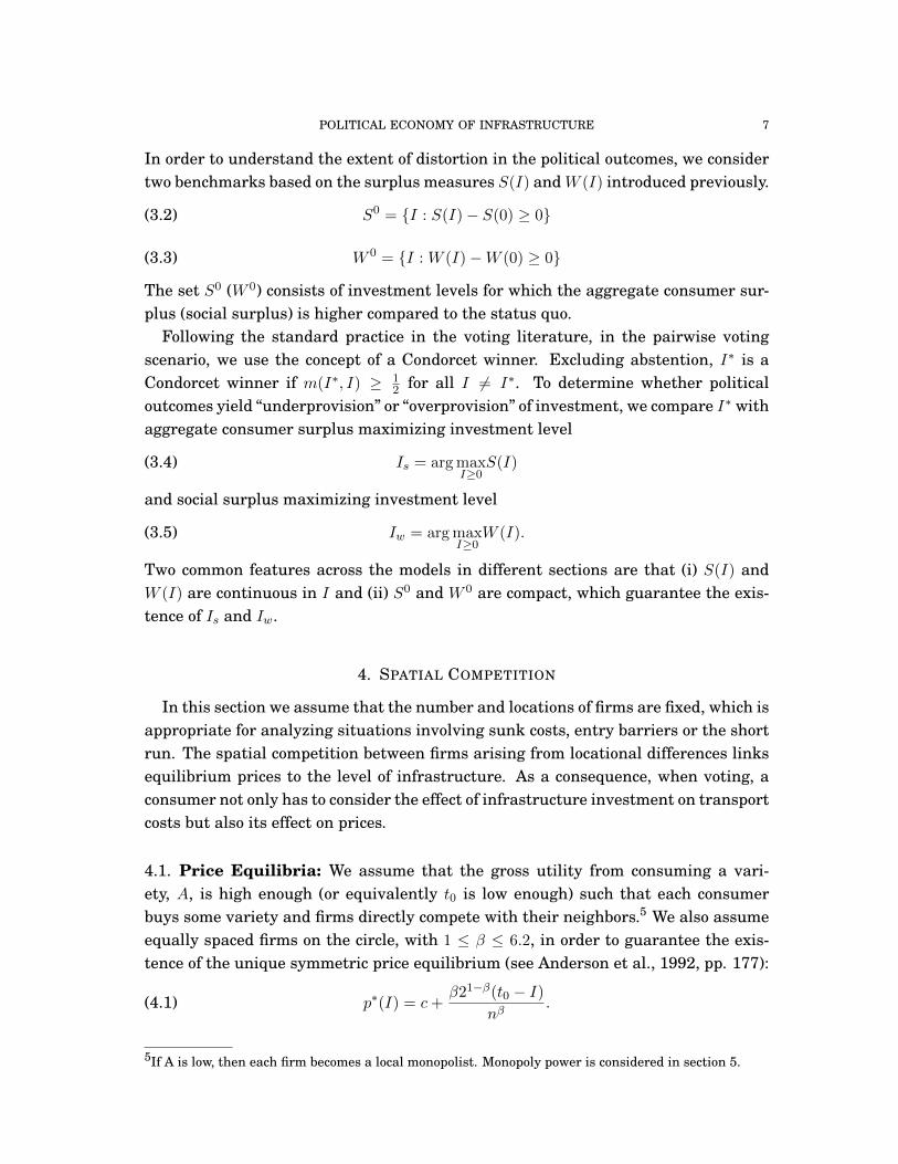
In order to understand the extent of distortion in the political outcomes, we considertwo benchmarks based on the surplus measures S(I) andW (I) introduced previously.

(3.2) S0 = {I : S(I)− S(0) ≥ 0}

(3.3) W 0 = {I : W (I)−W (0) ≥ 0}

The set S0 (W 0) consists of investment levels for which the aggregate consumer sur-plus (social surplus) is higher compared to the status quo.

Following the standard practice in the voting literature, in the pairwise votingscenario, we use the concept of a Condorcet winner. Excluding abstention, I∗ is aCondorcet winner if m(I∗, I) ≥ 1

2 for all I 6= I∗. To determine whether politicaloutcomes yield “underprovision” or “overprovision” of investment, we compare I∗ withaggregate consumer surplus maximizing investment level

(3.4) Is = arg maxI≥0

S(I)

and social surplus maximizing investment level

(3.5) Iw = arg maxI≥0

W (I).

Two common features across the models in different sections are that (i) S(I) andW (I) are continuous in I and (ii) S0 and W 0 are compact, which guarantee the exis-tence of Is and Iw.

4. SPATIAL COMPETITION

In this section we assume that the number and locations of firms are fixed, which isappropriate for analyzing situations involving sunk costs, entry barriers or the shortrun. The spatial competition between firms arising from locational differences linksequilibrium prices to the level of infrastructure. As a consequence, when voting, aconsumer not only has to consider the effect of infrastructure investment on transportcosts but also its effect on prices.

4.1. Price Equilibria: We assume that the gross utility from consuming a vari-ety, A, is high enough (or equivalently t0 is low enough) such that each consumerbuys some variety and firms directly compete with their neighbors.5 We also assumeequally spaced firms on the circle, with 1 ≤ β ≤ 6.2, in order to guarantee the exis-tence of the unique symmetric price equilibrium (see Anderson et al., 1992, pp. 177):

(4.1) p∗(I) = c+β21−β(t0 − I)

nβ.

5If A is low, then each firm becomes a local monopolist. Monopoly power is considered in section 5.


Note that p∗(I) is decreasing in I reflecting the fact that an increase in investmentlevel, i.e. a reduction in t, creates more competition among the existing firms, whichin turn leads to lower equilibrium prices.

4.2. Political Economy Results. Recall the individual surplus measure, s(y, I), in-troduced in section 2, substituting p = p∗(I) from equation (4.1), for a consumer y ∈ Cwe have:

(4.2) s(y, I) = A− p∗(I)− (t0 − I)|y − x∗i |β −γI2

2,

where x∗i is the location of the firm nearest to consumer y.Since the n firms are equally spaced around the circle and the equilibrium prices

are identical, it suffices to consider a mass of 12n consumers all located on one side of

a representative firm whose location is normalised to 0. A consumer y ∈ [0, 12n ] votes

against the status quo if

(4.3) s(y, I)− s(y, 0) = [p∗(0)− p∗(I)] + Iyβ − γI2

2≥ 0.

Observe that s(y, I) − s(y, 0) exhibits single crossing in y. Thus by an applicationof Gans and Smart (1996) the voting behavior of the median voter is sufficient todetermine the voting behavior of the majority.6 Noting that |y| = 1

4n is the medianconsumer, the set of investment level that beats the status quo in pairwise voting isgiven by:

R0 =

{I : s

(1

4n, I

)− s

(1

4n, 0

)≥ 0

}.(4.4)

Solving this inequality for I characterizes the investment levels which will win ina referendum. It also follows from single crossing and Gans and Smart (1996) thatthe most preferred investment level of the median consumer is the unique Condorcetwinner. The results are summarized in the following proposition.

Proposition 1. In a circular city model, with n ≥ 2 firms, voting on infrastructureinvestment yields the Condorcet winner I∗, where

I∗ =β21+β + 1

4βnβγ.

The set of investment R0 which dominate the status quo is R0 = [0, 2I∗]

By inspection I∗ is decreasing in γ and n. γ determines the rate at which marginalcost increases, thus quite naturally as the marginal cost of infrastructure increases,the equilibrium choice decreases.

6Also see pp 23, Chapter 2 in Persson and Tabellini (2000) for a definition and implication of the single-crossing property.


Increased n, an exogenous increase in the number of firms, lowers the distancetravelled by the median consumer which in turn reduces the direct marginal benefitfrom I. The indirect benefit of increased I, which operates through price reduction,i.e. d(p∗(0)−p∗(I))

dI = β21−β

nβ, is decreasing in n. Hence on both counts, the incentive to

invest becomes smaller as the number of firms increases.Finally, we turn to comparative statics with respect to β, the convexity of the

transport cost function. The direct marginal benefit of an increase in I is (4n)−β,which is decreasing in β. This is reinforced by the indirect effect, of price reduction,d(p∗(0)−p∗(I))

dI = 2β(2n)β

which becomes smaller as β increases. Thus I∗ is decreasing inβ.

4.3. Welfare Results. Substituting s(y, I) as given by equation (4.2) into the defini-tions of S and W gives

S(I) = A− p∗(I)− t0 − I(2n)β(1 + β)

− γI2

2,(4.5)

W (I) = A− c− t0 − I(2n)β(1 + β)

− γI2

2.(4.6)

We begin by determining S0 and W 0, respectively the set of I that improves ag-gregate consumer surplus and welfare compared to the status quo. Using equations(4.5) and (4.6) gives the following proposition.

Proposition 2. In a circular city model, with n ≥ 2 firms, the investment levels whichmaximize consumer surplus Is and welfare Iw are

Is =2β(1 + β) + 1

(2n)β(1 + β)γ,(4.7)

Iw =1

(2n)β(1 + β)γ.(4.8)

The set of investments which increases consumer surplus, over the status quo, is S0 =

[0, 2Is] and the set of investments which increases welfare is W 0 = [0, 2Iw]

Comparing W 0 and S0 it follows that W 0 ⊂ S0. The reasoning is simple. An in-crease in investment level increases S(I) through two channels - reduction in equilib-rium prices and reduction in aggregate transport costs. Change in price do not affectW (I). This implies that, corresponding to any change in I, the increase in W (I) isless than the increase in S(I) and accordingly any investment level that increases ag-gregate social surplus increases aggregate consumer surplus as well. In other words,W 0 ⊂ S0. This argument, appropriately modified, applies to marginal changes in I

too. Since marginal increase in W (I) is less than that of S(I), and W (I) and S(I)


are strictly concave, it follows that Iw < Is. A complete comparison of welfare andequilibrium outcomes is given by the following proposition.7

Proposition 3. In a circular city model, with n ≥ 2 firms, voting will lead to overinvestment:

Iw < I∗ ≤ Is(4.9)

W 0 ⊂ R0 ⊆ S0(4.10)

where equality holds only for β = 1.

The savings in transport costs for the median consumer, due to improved infras-tructure, is less than the average savings. This implies that there are investmentlevels I which increase S(I) but are not favored by the median consumer, and accord-ingly not supported by the majority. Hence R0 ⊆ S0. Since the savings are valuedsimilarly in W 0 and S0, the argument described above would suggest that R0 ⊆ W 0

as well. However, recall that the change in aggregate social surplus, W (I) −W (0),does not take into account the beneficial effect of price reduction due to improvedinfrastructure. This enlarges the set R0, and in fact for the specification chosen, itturns out that W 0 ⊂ R0. Similar arguments can be used to establish the ordering ofthe investment levels in (4.9).

5. COLLUSION

We take a simple approach to collusion in which the number of firms, n is fixed. Wederive the single price that firms set in the market, assuming they are able to colludeperfectly.8

Given the underlying symmetric structure of the model, there is a unique collusiveprice, which is increasing in I (as the following lemma shows).

Lemma 1. In a circular city model, with n ≥ 2 firms and A ≥ c + t(1+β)(2n)β

the uniquecollusive price is

pc(I) = A− (t0 − I)(1

2n)β.

This price is just high enough to reduce the utility of a marginal consumer —midway between two firms — to zero. The gross value of the product A is sufficientlyhigh, relative to costs, to make it unattractive for firms to set a price which excludesany consumer from the market.

In collusion, for pivotal consumers, the loss from increased price exactly offsets thegain from transport cost savings. All other consumers are made strictly worse off by

7Qualitatively Is(orIw) vary with n, β and γ in the same way was as I∗ does and the arguments aresimilar to those presented immediately after Proposition 3.8Implicit in this derivation is an assumption that discount rates are high enough to sustain collusion orthere exists some other collusive mechanism. The impact of infrastructure on the functioning of cartelsis left for future research.


improving infrastructure. This exploitative aspect of infrastructure under collusionleads to the following:

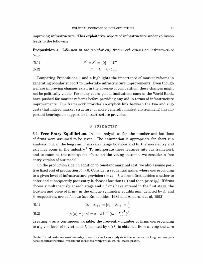
Proposition 4. Collusion in the circular city framework causes an infrastructuretrap:

R0 = S0 = {0} ⊂W 0(5.1)

I∗ = Is = 0 < Iw(5.2)

Comparing Propositions 1 and 4 highlights the importance of market reforms ingenerating popular support to undertake infrastructure improvements. Even thoughwelfare improving changes exist, in the absence of competition, those changes mightnot be politically viable. For many years, global institutions such as the World Bank,have pushed for market reforms before providing any aid in terms of infrastructureimprovements. Our framework provides an explicit link between the two and sug-gests that indeed market structure (or more generally market environment) has im-portant bearings on support for infrastructure provision.

6. FREE ENTRY

6.1. Free Entry Equilibrium. In our analysis so far, the number and locationsof firms were assumed to be given. The assumption is appropriate for short runanalysis, but, in the long run, firms can change locations and furthermore entry andexit may occur in the industry.9 To incorporate these features into our frameworkand to examine the consequent effects on the voting outcome, we consider a freeentry version of our model.

On the production side, in addition to constant marginal cost, we also assume posi-tive fixed cost of production K > 0. Consider a sequential game, where correspondingto a given level of infrastructure provision t = t0 − I, a firm i first decides whether toenter and subsequently post-entry it chooses location (xi) and then price (pi). If firmschoose simultaneously at each stage and n firms have entered in the first stage, thelocation and price of firm i in the unique symmetric equilibrium, denoted by xi andpi respectively, are as follows (see Economides, 1989 and Anderson et al, 1992):

|xi − xi+1| = |xi − xi−1| =1

n(6.1)

pi(n) = p(n) = c+ β21−β(t0 − I)(1

n)β.(6.2)

Treating n as a continuous variable, the free-entry number of firms correspondingto a given level of investment I, denoted by n∗(I) is obtained from solving the zero

9Note if fixed costs are sunk on entry, then the short run analysis is the same as the long run analysisbecause infrastructure investment increases competition which lowers profits.


profits condition (p(n)− c) 1n = K. This yields

(6.3) n∗(I) =

(β21−β(t0 − I)

K

) 11+β

.

For a given I ≥ 0, the subgame perfect Nash equilibrium outcome of the three-stagegame — entry (stage 1), location choice (stage 2) and price competition (stage 3) —can be summarized by a triplet (n∗(I), {x∗i (I)}n

∗(I)i=1 , p∗(I)) where n∗(I) is as in equation

(6.3), and x∗i (I) and p∗(I) are xi and pi respectively evaluated at n = n∗(I).

6.2. Welfare and Uncertainty. Suppose the initial level of infrastructure provisionin the economy is t = t0 and the number of firms, locations and prices are given byn∗(0), {x∗i (0)}n

∗(0)i=1 and p∗(0) respectively. While voting for I > 0, a consumer y cor-

rectly anticipates n∗(I) and p∗(I). However, since any equispaced location of n∗(I)

firms constitutes an equilibrium, a consumer computes the expected utility over allpossible distances |y−x∗i (I)| where x∗i (I) denotes the location of the nearest firm. As-suming a uniform prior for equilibrium distance |y−x∗i (I)| over the support [0, 1

2n∗(I) ],the expected surplus from an investment I > 0 is:

E[s(y, I)] = A− p∗(I)− (t0 − I)2n∗(I)

∫ y+ 12n∗(I)

y|y − xi|βdxi −

γI2

2

= A− p∗(I)− t0 − I(2n∗(I))β(1 + β)

− γI2

2,(6.4)

≡ S(I).

We use a constrained optimal approach to welfare in considering free entry—constrained in the sense that we take as given the way in which market forces deter-mine equilibrium prices and the equilibrium number of firms. This seems a naturalway to examine in isolation the distortions caused by the political process in deter-mining infrastructure investments.

Since s(y, I) = S(I) for all y on the circle C, and there is a unit mass of consumers,it follows that S(I) = S(I). Moreover, since profits are zero in free-entry equilibrium,the two aggregate surplus measures are equivalent: W (I) = S(I) = S(I) for all I > 0.This equivalence in turn implies that for all β ≥ 1,

W 0 = S0 ⊃ {0},(6.5)

Iw = Is = arg maxI≥0

S(I) > 0.(6.6)

As in the previous sections, the existence of strictly positive, surplus enhancing I,follows from the observation that infinitesimally small levels of I have zero cost andW (I) and S(I) are continuous in I for all I ≥ 0. However, those surplus enhancing Iare politically viable only if

S(I)− s(ymedian, 0) > 0,


where ymedian is the location of the median consumer. To check whether this inequal-ity holds, we first compute s(y, 0) and then identify the median consumer.

Note that if no investment is undertaken and the status quo is preserved it isnatural to assume that the firms maintain the initial locations. This yields

(6.7) s(y, 0) = A− p∗(0)− t0|y − x∗i (0)|β.

Since s(y, I) = S(I) for all y when I > 0, and s(y, 0) is decreasing in y it follows that

s(y, I)− s(y, 0) = S(I)− s(y, 0)

is increasing in y. Exploiting this, it can be shown that, I > 0 beats the status quo ifand only if the median consumer votes against the status quo. The relevant medianis the one with respect to initial equilibrium configuration, which means that themedian consumer(s) is located at distance 1

4n∗(0) from the nearest firm.

6.3. Political Economy Results. Having identified the relevant aspects of the pref-erences of voters, we now turn to some results. An interesting and somewhat surpris-ing property of the free entry model is the following threshold result.

Proposition 5 (Referendum Threshold). For all β > 1, there exists a thresholdI(β) > 0 such that investments below the threshold cannot beat the status quo in areferendum, i.e. if I < I(β) then I /∈ R0.

Infinitesimally small levels of investment decrease the transportation costs at eachlocation by an infinitesimal amount. At the same time, they cause firms to shiftin the long run so the median consumer now faces the average transportation costwhich is higher than the median transportation cost. As I → 0, p∗(I) → p∗(0) andn∗(I)→ n∗(0), implying that the indirect effects that work through price reduction orentry/exit are negligible. However, the negative effect of increased expected transportcosts arising as a result of switching from median to average does not vanish as longas β > 1. This in turn implies that unless the proposed investment level is higherthan a certain threshold ,it could not win a referendum. Thus, our referendum cangenerate an endogenous investment threshold — a feature which typically arises inthe presence of fixed costs and/or increasing returns. Also note that this thresholdfeature is only reflected in R0 and not in W 0 or S0 which once again highlights thequalitative differences between socially beneficial and politically viable outcomes.

Proposition 5 shows that I > 0 is politically viable only if I > I. On the otherhand, I cannot be too large either, since γ > 0. Let I(β) denote the upper bound ofpolitically viable investments. Indeed, if γ is suitably large there does not exist any Ithat satisfies both: I < I and I > I.

Proposition 6 (Free Entry Infrastructure Trap). For all β > 1 there exists a γ(β)

such that if γ > γ(β) there is an infrastructure trap: R0 = {0} and I∗ = 0.


Previously we showed that an infrastructure trap can arise due to collusion/monopoly,but here, the cause is different. The uncertainty regarding the distance ex post —inparticular the possibility that distance can increase — renders small changes polit-ically non-viable and if γ is suitably large, the moderate or high level of investmentlevels are not feasible either, leading to the “trap” or persistence of the status quo.

In the context of trade policy reforms in a competitive general equilibrium model,Fernandez and Rodrik (1991) obtained a bias for the status quo trade policy. Like ourtrap result, their status quo bias arises from individual specific uncertainty. How-ever, the context as well as the focus of their paper is quite different from ours. Forexample, market environment has little role to play in their model. Furthermore, thethreshold result (Proposition 5), offers a novel insight regarding the set of politicallyviable outcomes.

A comparison of the welfare optimal results and the political economy results isgiven in the following proposition for a strictly convex transport cost function.

Proposition 7. In a circular city model with free entry, if the transport cost functionis strictly convex (i.e. β > 1) then there exists γ(β) such that

(i) if γ ≤ γ(β) then {0} ⊂ R0 ⊂ S0 = W 0 and I∗ = Is = Iw > 0,(ii) while if γ > γ(β) then R0 = {0} ⊂ S0 = W 0 and I∗ = 0 < Is = Iw.

The relationships between S0 andW 0, Is and Iw as well as the “trap” for large γ (i.e.part (ii) of Proposition 7) has already been explained in this section. What remainsto be explained is the political outcome when γ is small, i.e. γ ≤ γ. Recall that, forI > 0, each individual’s (and hence the median voter’s) expected consumer surplusis the same as the consumer surplus for the population. This in turn implies thatthe political outcome from the electoral competition setting (i.e. Condorcet winner) issocially optimal, if there exists I that wins a referendum. Such I exists if γ ≤ γ.

Despite the identical point outcomes (i.e. I∗ = Is = Iw), the set of politically viableinvestments, R0, is strictly smaller than the set of welfare enhancing investments(S0 or W 0). The median transportation cost is lower than the average transportationcosts under t = t0 and accordingly the net benefit from a positive investment is valuedless by the median consumer. This explains the strict inclusion: R0 ⊂ B0 — theexistence of I that improves welfare and yet immiserizes the median consumer.

Finally, note that under linear transport costs and uniform distribution of con-sumers, socially desirable investments are also politically viable and vice versa.

Proposition 8 (Equivalence under Linearity). In a circular city model with freeentry, if the transport cost function is linear (i.e. β = 1) then R0 = S0 = W 0 andI∗ = Is = Iw > 0.

In this case, the median voter’s transport costs are the same as the average transportcosts and hence the median voter behaves in a socially optimal way.


7. CONCLUSION

Despite the importance of public infrastructure investments, theory, especiallywith regard to competition, is underdeveloped. We consider a spatial competitionmodel where we interpret the transport cost parameter as an index of infrastructure.By incorporating voting over infrastructure by consumers, we provide an explicit po-litical economy foundation for infrastructure investment. As one might expect, po-litical processes do not necessarily generate socially optimal or efficient outcomes.However, as our analysis shows, the source and magnitude of the inefficiency dependin subtle ways on the characteristics of the market environment.

We analyze a number of aspects of the market environment: market structure(competition versus collusion/monopoly); transport cost curvature (linear versus strictlyconvex); and entry (short run versus long run). Across the models, competition wasinfrastructure promoting (excessively so) while collusion and the uncertainty causedby free entry both led to infrastructure traps: choice of zero infrastructure investmentin a referendum or election where positive investment is socially optimal.

By focusing on consumers and voting, we have ignored the other side of the story:producers and the political apparatus they employ to protect their profits — lobbying.In the applied literature (e.g. trade policy literature) the presence of lobbying is oftencaptured by considering weighted social surplus as the objective function, with profitsbeing assigned higher weights than aggregate consumer surplus.10 Our preliminaryinvestigation suggests that inefficiencies and the possibility of an infrastructure trapexist under this setting as well.

Though we covered some distance in the analysis of market environments — com-petition, collusion and free entry— on the political economy front we have been moreselective. Two recent advances, in modelling electoral competition, which we do notconsider, are the citizen-candidate framework, a la Besley and Coate (1997) or Os-borne and Slivinski (1996) and the party competition approach of Roemer (2001) andLevy (2004). However, we would like to highlight the novelty our analysis offers byconsidering both point outcomes (e.g. electoral competition) as well as set outcomes(e.g. referendum outcomes). As we have shown, the referendum set can displayunique features which cannot be described with point outcomes (e.g. investmentthresholds). Also, the comparison between referendum and surplus enhancing setsdoes not necessarily mirror the results from the electoral competition setting. Forexample in Proposition 7(i), there is strict equality in the point outcomes, I∗ = Is,while the corresponding set outcomes do not exhibit equality, R0 ⊂ S0.

By endogenizing the transport cost parameter as a politically determined infras-tructure investment, we allow consumers, in their dual role as voters, to partially

10See Grossman and Helpman (1994) and Mitra (2001) for a microfoundation of this approach.


determine the environment they face when they make purchasing decisions. This ap-proach, of allowing consumers some role in choosing the “rules of the game”, appearsto produce a rich framework without a great deal of additional technical complexity.Our results highlight how market environment and political economy concerns cansubtly impact public investment in infrastructure.


APPENDIX

Proof of Proposition 1. Substituting equation (4.2) into the winning referendumequation (4.4) gives

(7.1) [p∗(0)− p∗(I)] +I

4nβ− γI2

2≥ 0.

Substituting the equilibrium prices from equation (4.1) gives

(7.2) I

[β21−β

(1

n

)β+

1

(4n)β− γI

2

]≥ 0.

Solving for I gives the expression for I∗ in Proposition 1. Note the upper bound on R0

is indeed positive if, as assumed, β ≥ 1. As the discussion preceeding the propositionshows the voting outcome is the median voter’s preferred policy, which is given by thefollowing:

I∗ = arg maxI∈R0

(s(1

4n, I)− s( 1

4n, 0))

=1

γ(β21−β(

1

n)β +

1

(4n)β)

=β21+β + 1

(4n)βγ

Since I∗ is the maximum of the same quadratic equation which defines R0 by twohorizontal intercepts it follows that I∗ is exactly half the upper bound of R0 (sincequadratic functions are symmetric).�

Proof of Proposition 2. By definition S0 := {I : I ≥ 0, S(I)− S(0) ≥ 0}. Using (4.5)it follows that

S(I)− S(0) = [p(0)− p∗(I)] + I(1

2nβ(1 + β)− γI

2)(7.3)

= I(β21−β(1

n)β +

1

(2n)β(1 + β)− γI

2),(7.4)

which is positive for all I ≤ 2γ (β21−β( 1

n)β + 1(2n)β(1+β)

). Hence

S0 := {I : 0 ≤ I ≤ 2

γ(β21−β(

1

n)β +

1

(2n)β(1 + β))} = {I : 0 ≤ I ≤ 2Is}

where

Is = arg maxI∈S0

S0 =1

γ(β21−β(

1

n)β +

1

(2n)β(1 + β)) =

2β(1 + β) + 1

(2n)β(1 + β)γ.

Similarly W 0 := {I : I ≥ 0,W (I)−W (0) ≥ 0}. Thus using equation (4.6) we find that

W 0 : = {I : 0 ≤ I ≤ 2

(2n)β(1 + β)γ} = {I : 0 ≤ I ≤ 2Iw}


where

Iw = arg maxI∈W 0

W 0 =1

(2n)β(1 + β)γ

�

Proof of Proposition 3. Direct substitution of β = 1 yields I∗ = 5/(4nγ) = Is, fromwhich the equality result follows immediately.

From propositions 1 and 2 the upper boundaries of the appropriate sets are simplydouble the correspond I value (with lower boundaries all zero). Hence it suffices toestablish the ranking of the I ’s. First comparing I∗ and Iw from propositions 1 and 2:

I∗ =β21+β + 1

4βnβγ≥ 1

(2n)β(1 + β)γ= Iw(7.5)

⇔ β21+β + 1

4β≥ 1

2β(1 + β)(7.6)

⇔ (β21+β + 1)(1 + β) > 2β.(7.7)

which holds for all β ≥ 1 since β21+β + 1 > 2β.Comparing I∗ and Is from propositions 1 and 2:

I∗ =β21+β + 1

4βnβγ≤ 2β(1 + β) + 1

(2n)β(1 + β)γ= Is(7.8)

⇔ 2β +1

2β≤ 2β +

1

1 + β,(7.9)

which holds because β ≥ 1.�

Proof of Lemma 1. Suppose n firms cooperatively set a single price p to maximizeindustry profits. The value of p that solves this maximization problem is the uniquecollusive price.

As firms have identical costs and are evenly dispersed around the circle C, maxi-mizing industry profits is equivalent to maximizing profit per firm. For a given p andt, each firm’s output and profit respectively are

q(p, t) = 2 min{(A− pt

)1β ,

1

2n},

π(p, t) = (p− c)q(p, t),

where min{(A−pt )1β , 1

2n} = (A−pt )

1β if market is not completely covered and 1

2n other-wise.

First consider p ∈ [A− t(2n)β

, A] for which q(p, t) = (A−pt )1β and consequently π(p, t) =

(p− c)(A−pt )1β . We have that

dπ(p, t)

dp= −(1 + β)(A− p)

1β−1

βt1β

[p− βA+ c

1 + β].


We find that A ≥ c + t(1+β)(2n)β

⇒ A − t(2n)β

> βA+c1+β ⇒ p − βA+c

1+β > 0 ⇔ dπ(p,t)dp < 0 for

all p ∈ [A − t(2n)β

, A]. This implies p = A − t(2n)β

maximizes π(p, t) in the intervalp ∈ [A − t

(2n)β, A]. Now consider p ≤ A − t

(2n)βfor which q(p, t) = 1

n . As q(p, t) isnot affected by p, π(p, t) is maximized at the highest possible price that satisfy p ≤A− t

(2n)βwhich is p = A− t

(2n)β. Thus at any given t, p = A− t

(2n)βmaximizes π(p, t)

which immediately implies that for all I ≥ 0, A− t0−I(2n)β

≡ pc(I) is the unique collusiveprice. �

Proof of Proposition 4. Substituting the collusive price pc into the change in indi-vidual surplus from equation (4.3) gives

(7.10) −I(

1

2n

)β+ Iyβ − γI2

2.

Now on the circle with n fixed we y ∈ [0, 12n ] thus yβ ≤

(12n

)β for all y since β ≥ 1.Thus the surplus change for any consumer from an increase in infrastructure un-der collusion is non-positive and strictly negative for all but the most distant con-sumer. Therefore all consumers are hurt by infrastructure improvements and henceR0 = S0 = {0} and I∗ = Is = 0. Notice the collusive price is just sufficient to ensurethat the most distant (lowest surplus from consumption) consumers still purchase.Thus under collusion all consumers still purchase and hence the effects of infrastruc-ture improvements on social welfare are the same as under competition just with adifferent distribution of benefits. Thus, as in proposition 2, W 0 6= {0} and Iw > 0.�

Proof of Proposition 5. Evaluating the median consumer’s change in net surplusfrom arbitrarily small levels of investment yields,

limI→0

(S(I)− s(x∗i +1

4n∗(0), 0)) = (S(0)− s(x∗i +

1

4n∗(0), 0))

= − t0(2n∗(0))β(1 + β)

(2β − 1− β)

< 0,

where the strict inequality follows from noting that 2β − 1− β > 0 for all β > 1. Thusfor a given β > 1, there exists I(β) such that no I < I(β) beats status quo. �

Proof of Proposition 6. Consider I > 0. I ∈ R0 requires

(7.11) s(ymedian, I)− s(ymedian, 0) = S(I)− s(ymedian, 0) ≥ 0.

where S(I) is the expected consumer surplus for median consumer (and in fact allconsumers). For a given β > 1, Let Imax(β) denote the value of I that maximizesS(I). Given the quadratic specification of cost of investment, i.e., γI2

2 , it is easy toshow that (i) Imax(β) > 0 and (ii) limγ→∞ Imax(β) = 0. The latter one , i.e. (ii), implythat for any given β > 1, there exists γ(β) large enough such that Imax(β) < I(β)


whenever γ > γ(β). Then the result follows from noting that no I < I(β) beats statusquo (Proposition 5).

Proof of Proposition 7. Summing s(y, 0), as given in equation (6.7) over y yields

S(0) =

∫y∈C

s(y, 0) = A− p∗(0)− t0(2n∗(0))β(1 + β)

Similarly

S(I) =

∫y∈C

s(y, I) = A− p∗(I)− t0 − I(2n∗(I))β(1 + β)

− γI2

2

Since n∗(I) and p∗(I) are continuous in I for all I ≥ 0, limI→0 S(I) − S(0) = 0. Fur-thermore, dS(I)dI |I=0 = 1

2n∗(0))β(1+β)> 0. This implies that there exists strictly positive

investment levels which increases aggregate consumer surplus. Also, since the twosurplus measures are equivalent, it follows that

W 0 = S0 ⊃ {0},(7.12)

Iw = Is = arg maxI≥0

S0 = arg maxI≥0

S(I) > 0(7.13)

Although expected utility from a positive level of investment is S(I) for all con-sumers the expected change in utility varies according to the initial transportationcost of each consumer. Since transport costs are convex, the transportation costs in-curred by the median consumer is lower than the average transportation costs in thestatus quo. Consequently, the average expected surplus is less than the surplus formedian consumers:

S(0) ≤ s(x∗i +1

4n∗(0), 0).

Since S(I) = S(I), we have that S(I) − S(0) ≥ S(I) − s(x∗i + 14n∗(0) , 0) which in turn

implies that S0 ⊇ R0, where equality only holds for β = 1.Note that since S(I) = S(I), the most preferred investment level for any consumer

y, amongst the strictly positive ones is arg maxI>0 S(I) = arg maxI>0 S(I) = Is. IfS(Is)− s(x∗i + 1

4n∗(0) , 0)) > 0 then Is = I∗. Else I∗ = 0 which occurs if γ is larger thana critical value, γ say. Obviously, when I∗ = 0, R0 = 0.�

Proof of Proposition 8. If transport costs are linear in distance, β = 1, then theexpected transport costs overall locations are the same as transport costs for themedian voter (in the uniform case the median voter is also the mean voter). Thus, inthe linear case the median voters preferences are the same as the social planner,s andhence the outcomes of the political process are equivalent to the appropriate welfareoptimal outcomes.�


REFERENCES

Aghion, P., Schankerman, M., 2004. On the welfare effects and political economy of competition-enhancing policies, Economic Journal 114, 800-24.

Aschauer, D. A., 1989. Is public expenditure productive? Journal of Monetary Economics 23,177-200.

Anderson, S.P, de Palma, A., Thisse, J.-F., 1992. Discrete choice theory of product differenti-ation, Cambridge, MA: MIT Press.

Anderson, S.P., Goeree, J.K., Ramer, R., 1997. Location, location, location. Journal of Eco-nomic Theory 77, 102-27.

Besley, T., Coate, S., 1997. An economic model of representative democracy, Quarterly Journalof Economics 112, 85-114.

Cadot, O., Roller, L.-H., Stephan, A., 2006. Contribution to productivity or pork barrel? Thetwo faces of infrastructure investment. Journal of Public Economics, 90(6-7):1133-53.

Catt, H., 1999, Democracy in practice, London and New York: Routledge.

Czernich, N., Falck, O., Kretschmer, T., Woessmann,L., 2011. Broadband infrastructure andeconomic growth, Economic Journal 121, 505-32.

Economides, N., 1989. Symmetric equilibrium existence and optimality in a differentiatedproduct market, Journal of Economic Theory 47, 178-94.

Felbermayr, G., 2007. International trade and the political economy of transport infrastruc-ture investment, mimeo, University of Tubingen.

Fernald, J., 1999. Roads to prosperity: assessing the link between public capital and produc-tivity, American Economic Review 89, 619-39.

Fernandez, R., Rodrik, D., 1991. Resistance to reform: Status quo bias in the presence ofindividual-specific uncertainty, American Economic Review 81, 1146-55.

Gabszewicz, J. J., Thisse,J.-F., 1992. Location, in R. J. Aumann and S. Hart, eds., Handbookof game theory, Vol. 1 Amsterdam: North Holland, 281-304.

Gans, J., Smart, M., 1996. Majority voting with single-crossing preferences, Journal of PublicEconomics 59, 219-37.

Ghosh, A., K.J. Meagher, and Ernie G.S. Teo, 2007, Full and federal integration of asymmetricnations, http://ssrn.com/abstract=1270478.

Grossman, G., Helpman, E., 1994, Protection for sale, American Economic Review 84, 833-50.

Hotelling, H., 1929. Stability in competition, Economic Journal 39, 41-57.

Jain, S., Mukand, S., 2003. Redistributive promises and the adoption of economic reform,American Economic Review 93, 256-64.

Knight, B., 2004. Parochial interests and the centralized provision of local public goods: evi-dence from Congressional voting on infrastructure projects, Journal of Public Economics88, 845-66.

Levy, G., 2004. A model of political parties, Journal of Economic Theory 115, pp. 250-77.

Majumdar, S., Mukand, S., 2004. Policy gambles, American Economic Review 94, 120722.


Meagher, K., Zauner. K., 2004. Product differentiation and location decisions under demanduncertainty. Journal of Economic Theory 117, 201-16.

Mitra, D., 1999. Endogenous lobby formation and endogenous protection: A long-run modelof trade policy determination, American Economic Review 89, 1116-34.

Osborne, M., Slivinski,A., 1996. Model of political competition with citizen-candidates, Quar-terly Journal of Economics 111, 65-96.

Persson, T., Tabellini, G., 2000. Political economics: Explaining economic policy, Cambridge,MA: MIT Press.

Productivity Commission, 1999. National Competition Policy-related infrastructural reforms”in Impact of Competition Policy Reforms on Rural and Regional Australia Inquiry Report,Australia: Pirion/ J.S.McMillan, 97 - 170. Also available athttp://www.pc.gov.au/inquiry/compol/finalreport/index.html

Roemer, J. E., 2001. Political competition: Theory and application, Cambridge MA: HarvardUniversity Press.

Roller, L., Waverman, L., 2001. Telecommunications infrastructure and economic develop-ment: A simultaneous approach, American Economic Review 91, 909-23.

Salop, S., 1979. Monopolistic competition with outside goods, Bell Journal of Economics, 10,141-56.

Winer, S.L., Hettich, W., 2008. Structure and coherence in the political economy of publicfinance, in B.R.Weingast and D.Wittman, eds., Oxford Handbook of Political Economy.

World Bank, 1994, World Bank Development Report 1994: Infrastructure for development,Oxford and New York: Oxford University Press.

SCHOOL OF ECONOMICS, UNIVERSITY OF NEW SOUTH WALES, SYDNEY, NSW 2052, AUSTRALIA.FAX:+61-2-9313 6337

E-mail address: [email protected]

RESEARCH SCHOOL OF ECONOMICS, AUSTRALIAN NATIONAL UNIVERSITY.E-mail address: [email protected]

the political economy of infrastructure …556.pdf · the political economy of infrastructure...

Documents