The Political Impact of the Internet in US

Presidential Elections∗

Valentino Larcinese† & Luke Miner‡

June 2017

Abstract

What are the political consequences of the diffusion of broadband internet? We

address this question by studying the 2008 US presidential election, the first politi-

cal campaign where the internet played a key role. Drawing on data from the FEC

and the FCC, we provide robust evidence that internet penetration in US counties

is associated with an increase in turnout, an increase in campaign contributions to

the Democrats and an increase in the share of Democratic vote. We then propose

an IV strategy to deal with potential endogeneity concerns: we exploit geographic

discontinuities along state borders with different right-of-way laws, which constitute

the main determinant of the cost of building new infrastructure. IV estimates con-

firm a positive impact of broadband diffusion on turnout, while the pro-Democratic

Party effect of the internet appears to be less robust.

Keywords: internet diffusion, political economy of the media, United States

elections, turnout, campaign contributions.

JEL Codes: D72, L82, L86

∗We are grateful for their useful comments to Oriana Bandiera, Tim Besley, Robin Burgess, BillCheswick, Ruben Durante, Greg Fischer, Maitreesh Ghatak, Steve Gibbons, Jason Ketola, Erik Kline,Alan Manning, Thomas J. Mather, George Michaelson, Henry Overman, and Gerard Padró i MiquelTorsten Persson, Steve Pischke, Jim Snyder, Piero Stanig, William Stevenson, Dimitri Szerman, TomVest. We greatly benefitted from presenting preliminary drafts of this papers at various conferences andworkshops, including APSA, EPSA, MPSA, PSPE, the Mass Media workshop at the EUI Florence andin seminars at Bocconi, Catholic University of Milan, EBRD, LSE, IRVAPP, Padova, Sciences Po. Weremain solely responsible for any errors.†Department of Government, London School of Economics, Houghton Street, London WC2A 2AE,

United Kingdom. email: v.larcinese@lse.ac.uk‡New Economic School, Moscow

1

1 Introduction

According to a survey conducted in February 2016 by the PEW Research Center,1 the

percentage of American adults who often get their news online is 38%. This is second

only to TV (57%) and larger than Radio (27%) or print news (20%). Among younger age

groups, 18-29 and 30-49, online news consumption actually exceeds TV news consumption.

Thus, it is unsurprising that a common theme has emerged in the U.S. press, expressed

succinctly by the Huffi ngton Post in the weeks after the 2008 presidential election: “were

it not for the internet, Barack Obama would not be president.”2 Similar claims were

made in the wake of the 2016 election crediting the proliferation of online “fake news”

for Donald Trump’s upset win. 3 At the same time, scholars are debating whether the

internet is responsible for the increased ideological polarization of American voters (see

for example Sunstein, 2001, and Gentzkow and Shapiro, 2011).

The presumption that the diffusion of broadband internet can have profound political

implications is certainly not limited to US politics. The use of internet censorship in

countries like China, for example, must be based on the presumption that free access to

some of the content available online can have political consequences. Alec Ross, , Hillary

Clinton’s senior political adviser at the US state department, compared the internet to a

“Che Guevara of the XXI century”. Speaking about the upsurge of democratic movements

in some Arab countries (the so-called “Arab spring”), he declared that “dictatorships

are now more vulnerable than ever as disaffected citizens organize influential protest

movements on Facebook and Twitter”.4 Robert McChesney, a leading communication

scholar, talks of a “communication revolution”providing yet unexplored opportunities for

democratic development and social reform.5

In this paper we provide evidence of the impact of internet broadband diffusion on

US presidential elections, with a special focus on the 2008 election. In many ways this

was a landmark election that transformed electoral campaigning strategies. As claimed

in the New York Times the day before the election took place, the 2008 presidential cam-

paign“has rewritten the rules on how to reach voters, raise money, organize supporters,

manage the news media, track and mold public opinion, and wage – and withstand –

1See Matsa and Lu (2016).2See Schiffman (2008).3See for example https://www.theguardian.com/commentisfree/2016/nov/14/fake-

news-donald-trump-election-alt-right-social-media-tech-companies.4The Guardian, June 22, 2011.5McChesney (2007).

2

political attacks, including many carried by blogs that did not exist four years ago”.6 Ac-

cording to Mark McKinnon, a senior adviser to George W. Bush’s presidential campaigns

“we’ll be analyzing this election for years as a seminal, transformative race”.7

Apart from the inherent importance of the 2008 election in US political history, there

are several empirical advantages to focusing on the first decade of the 2000s for under-

standing the impact of internet on politics. Following similar studies that have focused

on the availability of radio (Stromberg 2004 and Adena et al. 2015), television (Gentzkow

2006), or of specific cable channels like Fox News (DellaVigna and Kaplan 2007), it is

clear that periods where a new medium is introduced offer empirical advantages in iden-

tifying causal relationships. As shown by these papers, in order to identify a treatment

and a control group with aggregate observational data it is a necessary (although not

suffi cient) condition that only part of the population is reached by the new technology.

The period between 2004 and 2008 saw the largest growth in broadband penetration in

the US between any two presidential elections: hence comparing 2004 with 2008 creates

a pre-post difference for a large number of observational units. At the same time, focus-

ing on the 2004-08 period allows us to exploit a large geographic variation in internet

access or uptake. In subsequent years the market has become saturated, leaving little

variation to exploit for identification purposes.8 In particular, the availability of internet

on mobile phones means that there is now more widespread access opportunity and that

therefore broadband uptake is more likely to reflect individual characteristics rather than

external constraints. Exogenous constraints on supply (as opposed to variables affecting

demand) are key in identifying a causal effect of broadband diffusion rather than simple

correlations.

The 2008 race is also the first Presidential election that saw widespread usage of

internet as a campaigning tool. The Obama campaign’s online fundraising arm brought

in a record $500 million in small individual donations; and the campaign’s heavy use of

social media purportedly contributed to the highest rate of youth turnout since voting

was extended to 18-year-olds.

We test the extent to which these assertions hold, looking at the effect of internet

diffusion on campaign contributions, turnout and vote share in the 2008 election. Our

analysis is conducted at the county level, for which we assemble a dataset of political

outcomes, combining presidential vote data with turnout and a full record of campaign

6Nagourney (2008).7Nagourney (2008).8See Horrigan and Duncan (2015)

3

contributions.

A study of this sort poses two formidable obstacles: 1) how to reliably measure internet

penetration at a suffi ciently detailed level; 2) endogeneity of internet penetration could

lead to correlations with the variables of interest, which do not accurately reflect causation.

Our first contribution is to propose a solution for the measurement problem by devel-

oping a proxy for internet usage over the 1999-2008 period. Unfortunately until December

2008 there was no publicly available data on internet usage in the U.S. at anything below

the state level. We develop a county-level proxy, using data on the number of high speed

Internet Service Providers (ISP) that were registered with the Federal Communication

Commission (FCC) in a zip code. We test this proxy against state-level measures and

find a high correlation. We also show that the number of high speed ISPs and the number

of broadband residential lines are highly correlated at the county level in 2008 (i.e. the

first year when both are available at the county level) and 2012.

Armed with this proxy for internet penetration we report difference-in-difference re-

sults using county-level changes in our outcomes of interest between 2004 and 2008.9 This

methodology, however, can only partially address the problem of endogeneity in internet

penetration. Ideally we would like to observe and compare counties which are equal in

all relevant characteristics, but that happen to have different internet uptake for reasons

that do not depend on voters’characteristics. For this purpose it is necessary to sep-

arate demand and supply of internet services and find instances of exogenous shifts in

the supply curve. To accomplish this task we exploit geographic discontinuities along

state borders with different right-of-way laws. We argue that right-of-ways laws provide

an exogenous source of variation in the cost of building internet infrastructure, hence

exogenously affecting broadband penetration in the US counties.

We compare counties on either side of state borders, whose unobserved characteristics

should be spatially correlated. By taking the difference between contiguous counties

on either side of the border and instrumenting by right-of-way laws, our methodology

controls for unobserved characteristics, providing us with estimates of the causal effect of

broadband internet growth on the outcomes of interest.10

Our findings are mixed. We find a strong effect of internet access on share of the vote

going to the Democratic candidate in our OLS estimates but this effect vanishes when we

use IV, suggesting the presence of a co-movement between broadband penetration and

9We will also show some results for the period between 2000 and 2004.10In our use of spatial differencing to control for unobserved characteristics, our empir-ical methodology is similar to that of Duranton et al (2011).

4

Democratic vote which is not causal. We find instead that the internet had a positive

effect on turnout in 2008. This effect is robust in both OLS and IV estimates and holds

across a number of specifications. We also find some evidence of an effect on campaign

contributions for the Democratic candidate.

2 Related literature

This study makes a number of contributions and can be related to several streams of

existing research. First, it provides some of the first quantitative evidence of the role of

the internet in U.S. elections. There is only limited quantitative large-N research in this

area and very few papers have explored the electoral impact of the internet while credibly

addressing causal identification concerns. Falck et al (2014) find that the availability of

the internet in Germany had a negative impact on electoral turnout. Campante et al.

(2013) also find a sizeable negative impact of broadband diffusion on turnout in Italy.

They also find, however, that the initial negative impact was reversed in 2013 when the

anti-establishment Five Star Movement ran in the general election. Gavazza et al. (2016)

find that internet penetration reduced turnout in the United Kingdom. They also show

that broadband diffusion is correlated with various local government policies concerning

taxation and expenditures. Miner (2015), on the other hand, finds that internet pene-

tration in Malaysia increased turnout and had a general anti-incumbency effect. Positive

effects on turnout have also been found by Poy and Shuller (2016) in their study of the

Trento province in Italy. Other papers have related internet diffusion with an increase

in social capital in Germany (Bauernschuster et al. 2014), reduced corruption in the

US (Andersen et al. 2011), and have shown that the usage of social media can increase

accountability when traditional media are not independent (Enikolopov et al 2016).

In the case of the US, correlations between internet usage and political engagement

are well documented, although with mixed results. Tolbert and Mcneal (2003) and Moss-

berger, Tolbert, and McNeal (2008) report a positive correlation between reading news

online and turnout using, respectively, data from the American National Election Study

and PEW’s Internet and American Life Survey. On the other hand, Bimber (2001),

Baumgartner & Morris (2010) and Hargittai & Shaw (2013) find no correlation. Some

research on US ideological polarization has been inspired by the seminal work of Sunstein

(2001), claiming that the internet favors the creation of echo chambers where people are

predominantly exposed to views similar to those they already have, increasing ideological

segregation and the polarization of the American electorate. Nie et al. (2010) provide

5

some support for Sunstein’s echo chamber hypothesis by showing that people tend to

use the internet in a selective fashion, i.e. exposing themselves to similar political views.

However, this is only a necessary condition for increasing polarization. Gentzkow and

Shapiro (2011) use survey data to show that online news consumption is not associated

with higher ideological segregation than offl ine news.

Our paper is the first to offer causal estimates of Internet penetration in the US on

various political outcomes. Moreover, in this paper we propose an identification strategy

that can potentially be broadly applied to study the political and social impact of broad-

band diffusion.11 From a methodological point of view our paper relates to a growing

literature that employs spatial econometrics to achieve identification. Particularly related

is a paper by Naidu (2012), who estimates the effect of 19th century disenfranchisement

of African Americans in the U.S. South, comparing adjacent county-pairs on state bound-

aries. Dube et al (2010) use the same methodology in an earlier paper to estimate the

effects of minimum wages on earnings. Our paper employs a different method in which

the cross border comparison of adjacent county-pairs is supplemented by an instrumental

variable approach.

3 Background

3.1 Personal Use of Internet

Internet use in the US has grown enormously from 16% in 1996 to 74% in 2008, with the

latest percentage available (2015) at 75%.12 This growth masks an even greater change

in the method and sophistication of usage over this period of time. In 1996, AOL was

still one of the main methods of accessing the internet, meaning relatively few people

left its portal, which was effectively a walled garden of curated and licensed content.

Moreover, most connections were dial-up and too slow to display video content. Modern

social networks did not yet exist. Bill Clinton did have his own web-page during the 1996

campaign, but it was small, with none of the fundraising and organizational tools that we

see in modern campaigns.13 Unsurprisingly, only a small fraction of the voting population

11See for example the paper by Lelkes et al (2017). Following our identification strategyLelkes et al. (2017) show that internet diffusion increases the consumption of partisanmedia and is, via this channel, a likely cause of increased polarization.12Yearly data is available from the World Bank and from the International Telecom-munication Union.13See www.4president.us/websites/1996/clintongore1996website.htm

6

used the internet for political ends, 4% according to a Pew study.14 In contrast, the same

study found that as of 2008 a full 44% of the adult population used the internet as a

source of political information, and that it was the primary source of political information

for 30% of the population.

Although the stereotype holds that a typical Obama supporter was more wired than

a McCain supporter, in practice the opposite is the case: 83% of McCain supporters were

internet consumers as opposed to 76% of Obama supporters.15 However, much of this is

explainable by the gap in average income and education between the two groups. More-

over, whereas the average McCain voter might be more connected, the average Obama

voter was more likely to use the internet to political ends. Nowhere is this more evident

than in the case of young voters aged 18-29, who, at 72%, were the most politically ac-

tive online of all age groups.16 They also swung disproportionately to Obama: 66% of

the youth vote went to Obama in 2008 as opposed to 54% to Kerry in 2004.17 More-

over, turnout among the youth was the highest on record since voting was extended to

18-year-olds in 1972.18

3.2 Campaign Use of the Internet

3.2.1 New Media

The Obama campaign exploited the internet in a number of ways. First, they made

ample use of social media to further their cause both through Facebook and the campaign

website my.barackobama.com (MyBO). These tools helped augment traditional campaign

tactics: detailed information on supporters helped improve mobilization, especially during

caucuses; MyBO supplied tools allowing volunteers to make calls on the campaign’s behalf

from home; and MyBO and Facebook centered tools also helped volunteers organize their

own fundraising events, connecting with friends they hadn’t seen for years.19 The Obama

campaign’s aggressive action in the social media space played out in exit-survey data.

According to PEW, 25% of Obama supporters used social networks for political ends as

opposed to 16% of McCain supporters.20

14See Smith and Rainie (2008) p.5.15See Smith and Rainie (2008) p.10.16The number drops to 65% for people aged 30-49, 51% for 50-64, and 22% for 65+.For additional details see Smith and Rainie (2008) p.17.17See Keeter, Horowitz and Tyson (2008).18See Falcone (2008).19See Talbot (2008).20See Smith and Rainie (2008) p.11.

7

The Obama campaign also used online video to get their message to a large audience

without having to pay the traditional advertising costs of television. For example, a video

of Obama’s speech on race relations got 6.7 million views by November 2008.21 Again

this translated into a gap among supporters: 21% of Obama supporters shared political

videos as opposed to 16% of McCain voters.22

All of these trends were especially pronounced among young voters aged 18-29, the

largest users of all types of social and online media: 67% of young voters reported watching

online political videos; and 49% used social networks politically, with 40% posting original

online content relating to the campaign.23

3.2.2 Fundraising

The area of Obama’s online campaign that has received the most attention is fundrais-

ing, where the campaign brought in an estimated 500 million dollars in online donations,

eclipsing Howard Dean’s previous record of 27 million. In fact the technology used for

Obama’s online fundraising was developed by veterans of the Dean campaign, a company

called Blue State Digital. They built a number of tools to make the effort more “social”:

people could set their own personal targets; run fundraising campaigns; and watch per-

sonal thermometers rise, which gauged how well they met their targets.24 The results in

terms of exit polls is dramatic: Pew reports that 15% of Obama voters donated online in

contrast to 6% of McCain voters.25. The results are equally striking in terms of type of

donation: of the 6.5 million donations online, 6 million were in increments less than $100

and often from the same person.26

3.3 Expected Outcomes

Online engagement with politics is only possible if access to internet at a suffi ciently high

speed is available. Our empirical investigation will therefore provide evidence on the causal

effect of broadband diffusion in the US counties on outcomes that, for reasons outlined in

the above sections, we expect to have been affected by voters’internet usage. In particular

we expect that broadband diffusion should: 1) increase donations for the 2008 Democratic

21“How Obama’s Internet Campaign Changed Politics”, New York Times 7 Nov. 2008(by Claire Miller)22See Smith and Rainie (2008) p.11.23See Smith and Rainie (2008) p.17.24For more details, see Talbot (2008).25See Smith and Rainie (2008) p.11.26See Vargas (2008).

8

candidate; this increase should be particularly strong among small donations (less than

$500 dollars), due to the Obama campaign’s use of its online portal to collect a record

amount of small-scale donations; 2) increase turnout, in particular among youth, since

the Obama campaign employed extensive tools for interacting with and mobilizing voters,

and usage of these tools was highest among people aged 18-29; 3) increase support for the

Democratic candidate, due to the tools used by the Obama campaign both to convince

swing voters (e.g. via video) and mobilize voters in general.

4 Data

4.1 Internet Data

The Federal Communication Commission began collecting detailed information on broad-

band penetration in December 1999. Figure 1 shows the evolution over time of fixed-

location connections in the period 1999-2012. If we take any two consecutive presidential

elections in the period 1996-2012 (setting 1996 level at zero), 2004-08 was the period which

saw the fastest increase in the number of residential connections, which rose from about

20 to around 75 million in just four years. By 2012 residential fixed connections had only

grown by another 10 million.27 Figure 2, from the PEW research center, uses survey data

to show internet access by American adults and leads us to similar conclusions.

It is therefore not by chance that 2008 is the first election to witness a massive usage

of internet for presidential electoral campaigning. This in itself, and irrespective of the

anecdotal evidence we have reported, justifies our choice of basing our analysis of the

political effects of the internet on a comparison between the 2004 and 2008 elections.

Unfortunately, until December 2008 the U.S. lacked comprehensive, publicly available

data on broadband usage and availability at anything finer than the state level. ISPs

27Further details are available from the FCC web page. It should be noted that weare not claiming that broadband has not grown both in quantity and quality since 2008:while fixed-line connections have grown at a reduced pace, mobile connections have be-come much more diffuse and the connection speed, both upstream and downstream, hasimproved substantially, especially in some areas. An increased number of mobile connec-tions, however, does not mean that as many people gained access to internet, as insteadwas the case when residential fixed lines were first installed. According to the Interna-tional Telecommunication Union, for example, the number of people using internet hasbarely changed between 2008 and 2015. Moreover, focussing on fixed-location connectionsand on a period with limited mobile access to the internet gives us another empirical ad-vantage, namely that it’s easier to locate users and link observations to specific zip codes,a feature that will prove useful in our analysis.

9

don’t release private information on subscribers due to its proprietary nature, and survey

data is scant. We therefore use a common alternative proxy for broadband usage: the

number of broadband providers operating in a zip code.

This data was collected by the FCC’s Form 477 on a semi-annual basis for the 1999-

2010 period from all high-speed providers with more than 250 high-speed lines in a state.

A provider is counted as high speed if transfer speed is greater than 200 kilobits per

second in at least one direction. The data does not differentiate between cable, DSL,

satellite, residential, or business providers. A provider is counted if they have at least

one subscriber in a zip code. Figure 3 illustrates on a map the number of ISPs operating

in each zip code at the beginning of the period we study (June 2004). Our measure is

obtained by averaging at the county level the number of ISPs operating in each zip code,

where the average is weighted by the population of each zip code.28

There are a number of reasons that this is a good proxy for internet take-up. In

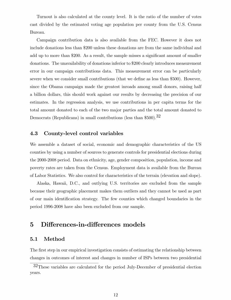
Table 1 we use available state-level data from FCC to regress the logarithm of high-speed

lines per capita on the logarithm of providers for the 48 contiguous states for the period

1999-2008. As can be seen in specification (1), even without controlling for population

or state-year fixed effects, the relationship between the log of providers and the log of

high-speed lines is positive and highly statistically significant with an R-squared of .54.

The strength of this relationship is unaffected by introducing a control for population

in specification (2). In specifications (3) and (4) state-year fixed effects are introduced,

barely affecting the coeffi cient on log providers and yielding markedly higher within R-

squared values. Specification (3) can be seen graphically in Figure 4, which shows a strong

positive relationship apart from three outliers in the bottom right corner. In specifications

(5) and (6) we drop these outliers, yielding a far more significant relationship and, in the

last case, a within R-squared of .96.

One concern is that this relationship could be far less significant at the county level.

Fortunately, as of December 2008, the FCC reports broadband take-up at the county level,

so that we can check how our measure correlates with the number of residential lines at the

end of the period of study. Figure 5 reports fitted values of a fourth polynomial regression

of subscribers on providers in December 2008, showing a robust positive correlation. This

graph is based on a coarse description of broadband uptake, since the FCC only reported

the data bracketed into 6 categories, from 0 (lowest) to 5 (highest). In 2012 the FCC

28Since the number of providers in zip codes with less than three providers but morethan zero is not reported for confidentiality reasons, we assume that all these zip codeshave two poviders.

10

conducted a more detailed investigation reporting the county-level number of individuals

with no access to broadband, from which we can derive the number of individuals with

access. Once again, a fourth polynomial regression displays an increasing relationship

between the number of providers and the percentage of population with broadband ac-

cess (Figure 6). The relationship is concave and becomes less precisely estimated at the

extremes of the distributions of providers, where the number of observations is small.29

A kernel density estimate of the distribution of providers in the US counties in 2008 is

reported in Figure 7.

The evolution of our main explanatory variable between 2000 and 2008 is shown in

Figure 8. Although the relationship between number of providers and internet take-up is

significant, there are several factors that introduce measurement error. The main concern

is that this measure may only be proxying for the competitiveness of ISP markets in a

county. Although this will certainly introduce error, the strong correlation that we find

between the number of ISPs and high-speed internet adoption reassures us that there will

still be substantial variation related to internet usage. Also, high-speed internet does not

include dial-up connections, although this should be only a minor concern in the period

we study.30

4.2 Political Data

All political variables are likewise available at the county level, covering presidential elec-

tions for the period of interest. Variables on absolute number of votes are derived from

FEC data.31 This allows us to derive a measure of Democratic and Republican vote share

for each presidential election.

29Kolko (2010) analyzes the relationship between high-speed Internet adoption and thenumber of providers at the zip code level, using zip-code level survey data from Forresterand also finds a strong positive, monotonic relationship between the number of providersin a zip code and its level of high-speed Internet take-up. The only outliers are at theextremes of the distribution for which there are very few observations.30According to survey data of the PEW Research Center, in 2004 about 30% of Ameri-can adults accessed Internet using dial-up. This share declines to 10% in 2008. Assumingthat most of this variation constitutes a switch to broadband, this upgrade is part of whatour broadband intake proxy tries to capture. The fact that some 2008 broadband usersused dial up in 2004 (rather than not using Internet at all) should, if anything, bias theeffects of broadband adoption downwards. There remains a 10% of Internet users whichis not captured by our indicator and this also should bias our results downwards. In anyevent, we don’t think this will introduce much error into our results, mostly because,given the speed limitations inherent in dial-up, many of the modern techniques employedby campaigns such as video streaming are not available.31See David Leip’s Election Atlas at uselectionatlas.org

11

Turnout is also calculated at the county level. It is the ratio of the number of votes

cast divided by the estimated voting age population per county from the U.S. Census

Bureau.

Campaign contribution data is also available from the FEC. However it does not

include donations less than $200 unless these donations are from the same individual and

add up to more than $200. As a result, the sample misses a significant amount of smaller

donations. The unavailability of donations inferior to $200 clearly introduces measurement

error in our campaign contributions data. This measurement error can be particularly

severe when we consider small contributions (that we define as less than $500). However,

since the Obama campaign made the greatest inroads among small donors, raising half

a billion dollars, this should work against our results by decreasing the precision of our

estimates. In the regression analysis, we use contributions in per capita terms for the

total amount donated to each of the two major parties and the total amount donated to

Democrats (Republicans) in small contributions (less than $500).32

4.3 County-level control variables

We assemble a dataset of social, economic and demographic characteristics of the US

counties by using a number of sources to generate controls for presidential elections during

the 2000-2008 period. Data on ethnicity, age, gender composition, population, income and

poverty rates are taken from the Census. Employment data is available from the Bureau

of Labor Statistics. We also control for characteristics of the terrain (elevation and slope).

Alaska, Hawaii, D.C., and outlying U.S. territories are excluded from the sample

because their geographic placement makes them outliers and they cannot be used as part

of our main identification strategy. The few counties which changed boundaries in the

period 1996-2008 have also been excluded from our sample.

5 Differences-in-differences models

5.1 Method

The first step in our empirical investigation consists of estimating the relationship between

changes in outcomes of interest and changes in number of ISPs between two presidential

32These variables are calculated for the period July-December of presidential electionyears.

12

elections. We focus on the 2004-08 period but also report estimates for 2000-04. We

estimate equations of the form:

∆yis = αs + β∆Ii + γ∆Zi + εis (1)

where yis is an outcome variable in county i and state s (voting shares of Democrats

or Republicans, turnout and campaign contributions), Ii is our proxy for internet take-up

(number of providers) in county i, Z is a vector of control variables and εis is an error

term. As customary, we indicate with ∆ the difference between the 2008 and 2004 (2004

and 2000) values of a variable. Since our dependent variable is expressed as county-level

difference, a simple regression controls for all county-specific time invariant confounding

factors and corresponds to a standard fixed effects specification. Including state fixed

effects in this specification accounts for state-specific shocks, i.e. anything that might

have changed at the state level between the two elections, which is important since states

are the relevant battleground in presidential elections. We include the following control

variables: population characteristics (population density, percentage of voters aged 18-29,

percentage of population above 65, percentage male, percentage of black, hispanic, asian

residents), income levels (poverty rates, average individual income), education (percentage

with a college degree). In our most demanding specification

∆yis = αs + β∆Ii + γ∆Zi + δZit + εis (2)

we also include our control variables at their first period level (i.e. 2004 level if the∆ refers

to 2004-08). It should be noted that including these level-variables together with their

∆s serves a more demanding purpose than simply controlling for those omitted factors.

Since the dependent variable is a difference, by including control variables expressed in

levels we are accounting for the possibility that different pre-existing characteristics were

affecting the trends in the outcome of interest across the counties. In this specification

we also include characteristics of the terrain, namely average slope and elevation and the

standard deviation of the county elevation. The standard errors we report are always

clustered at the state level. As usual with this sort of specification the main concern is

represented by confounding factors that change over time. While we control for a large

set of county characteristics, we should still be concerned about possible bias generated

by unobservable omitted variables.

13

5.2 Results

Table 2 reports the results of the effects on turnout and vote share for the Democratic

party. Results for Republican vote share are almost exactly the opposite of what we find

for the Democrats. For the period 2004-08 (panel A) there is a robust correlation between

the increase in number of providers and both the vote share of the Democratic candidate

and voter turnout. This correlation also holds in the more demanding specifications

of columns 4 and 8 where we introduce control variables at their 2004 levels, although

the magnitude is substantially reduced. In our preferred specification (columns 3 and

7), which corresponds to a county-fixed effect regression with state-specific shocks, an

increase in the number of providers by one standard deviation above the average (1.89)

corresponds to about 0.67% increase in the percentage of Democratic vote and 0.31%

increase in turnout. In the most conservative specifications (columns 4 and 8) these

effects drop respectively to 0.21% and 0.13%.

The bottom panel of the table reports results for the 2000-2004 period, i.e. when

both the dependent and independent variables refer to the previous electoral cycle. The

pattern that emerges from the 2000-04 period is similar to that of 2004-08 but less robust,

particularly for the share of the Democratic vote. For voting returns, the results with

state specific shocks are comparable to those of the top panel but vanish when we include

control variables. For turnout the results are similar to the 2004-08 case, although sta-

tistically insignificant when control variables are included. If these coeffi cients could, at

least in part, capture a causal effect, then we should conclude that the mobilizing effect

of the internet on turnout was, to a certain extent, already present before the Obama

campaign but that the partisan pro-Democrat effect was probably not. To better un-

derstand the difference between panel A and panel B it is important to stress that the

main explanatory variable in the two periods has a correlation coeffi cient of -0.015. In

other words the counties with fastest broadband diffusion in 2004-08 are not the same

that experienced broadband diffusion in 2000-04. The fact that in both periods we find a

positive association between broadband diffusion and our electoral outcomes is therefore

unlikely to be due to specific county characteristics.

In Table 3 we report diff-in-diff estimates for campaign contributions.33 Again we

uncover a pro-Democrat effect of internet penetration in the form of increased campaign

contributions, while no effect is detected for contributions to Republicans. The effect this

time appears to be stronger in 2000-04 but the magnitudes for the two periods are similar

33In the interest of space we do not report the simple regression of outcomes overproviders.

14

when all controls (both in differences and in levels) are included. Magnitudes are also

similar both for overall contributions and for contributions below 500 dollars.

Our diff-in-diff estimates show a robust correlation between broadband diffusion and

increase in turnout in presidential elections. They also suggest that the internet might have

had a pro-Democrat effect in its early days, both in terms of vote shares and campaign

contributions. This is not surprising since both in 2004 and in 2008 the Democrats were

ahead of the Republicans in exploiting the new medium, as we documented in Section 3.

These estimates take us a long way in identification terms since they take into ac-

count fixed county-specific characteristics, state-specific shocks (particularly important in

presidential elections) and a number of observable county variables that change over time.

Nevertheless, these estimates would still be biased if there were unobservable county char-

acteristics that changed between two elections and that could be related to both broad-

band diffusion and our variables of interest. For example, Stephens-Davidowitz (2011)

provides evidence that racism played a large role in the outcome of the 2008 election. If

racism was on the decline in areas with more internet penetration, our results would be

overestimated. For this reason in the next section we propose an identification strategy

based on a source of exogenous variation in internet penetration.

6 Instrumental variable: Right-of-Way Regulations

6.1 The ROW Data

First-order identification concerns come from the fact that political behavior and attitudes

could be correlated to the demand for internet services. Correlations between broadband

adoption and political variables could then simply be the consequence of the fact that

different type of individuals live in different counties. Although diff-in-diff estimates take

this problem into account if these differences are fixed or moving slowly (for example

people more interested in politics and more likely to vote could also be more interested in

surfing the net), this remains a concern if these same characteristics changed suffi ciently

rapidly, i.e. in the space of four years between two presidential elections. An exogenous

source of variation in broadband diffusion must then be found in the non-demand related

part of the supply of internet, i.e. when broadband availability is constrained by variables

which are not related to the demand side.

When taking decisions about the roll out of infrastructure, internet providers consider

the profitability of alternative investments, comparing the costs with the potential rev-

15

enue. Although the most important variables are likely to be population density and co-

variates which determine the demand for internet services (for example education, wealth,

age etc.), different levels of broadband penetration across the US states can be attributed

in part to different regulatory regimes concerning Right-of-Ways (ROW) laws (see Day,

2002). These can be broken down into a number of different items, which influence the

cost for ISPs to lay infrastructure:34

1. Jurisdiction: In some states, an ISP has to get permission to build on the public

ROW from every single municipality that the project crosses, whereas in other states this

is handled by a centralized authority.

2. Compensation: Compensation demanded by municipalities in return for granting

ROW permission ranges from cost recovery (the cost to the municipality of administering

the ROW) to a rental fee (e.g. percentage of gross revenue) to a flat tax.

3. Timeliness: Some states have a maximum time for processing permit applications,

significantly speeding up the process.

4. Mediation and Condemnation: States also vary in how they deal with conflicts

between municipalities and ISPs, and private landowners and ISPs. For example, in Ver-

mont, landowner complaints can be heard on a wide range of issues including aesthetics,

and decisions are appealable to the Vermont Supreme Court. On the other extreme is

Texas, where most factors are not appealable and landowners must pay the ISPs legal

expenses if they lose in court.

5. Remediation and Maintenance: These laws dictate issues such as in what state of

repair ISPs must maintain their facilities. For example, if a sidewalk is torn in order to

lay cabling, these laws determine to what extent the sidewalk would need to be restored

to its original state and under what time frame.

Historically, municipal ROW laws can be dated back to a different era, when they

served the purpose of regulating the roll out of electricity and telephone infrastructure.

The current ROW regime has been re-defined by the Telecommunications Act of 1996,

which allowed municipalities to regulate the public ROW, hence leaving many pre-existing

laws in place.35

States also passed their own laws concurrent with the Telecommunications Act that

either limited or reinforced this municipal right, leading to the significant variation in

34See NARUC (2002) for more details.35Section 253(c) of the Act states: “ Nothing in this section affects the authority of aState or local government to manage the rights-of-way or to require fair and reasonablecompensation from telecommunication providers, on a competitively neutral and non-discriminatory basis”.

16

ROW regulations across states that we see today. For example, the time frame within

which a local government must respond to a request to use its rights-of-way has been fixed

to 30 days in Ohio, 90 days in Michigan and 120 days inWashington. Most states, however,

decided to impose no limit. When states opt for a light-touch regulation the consequence

is often that “each municipality may have its own policies, impose separate requirement or

fees, and take different lengths of time to grant permits. This inconsistency across a state

makes it very diffi cult to plan a coherent network rollout” (Kende and Analysys, 2002).

Some municipalities regulate the hours that a telecom provider must be available to take

customer complaints and the time-frame in which new customer orders must be filed.

Some municipalities require having a customer care offi ce in the municipality. According

to Day (2002) “A number of municipalities continue to block ROW access as a means of

extracting additional compensation from telecommunication providers”.36

According to the National Telecommunication and Information Administration the

consequence of the current regulatory regime is that “rights-of-way management has

arisen as a key issue in broadband deployment at the federal, state, and local levels. The

steps required for a telephone company to lay new lines on a public street, a cable com-

pany to start providing internet service, or a cell phone company to place antennas on

public poles, can have real consequences in the decision to deploy broadband service to a

community.”37

In 2002 TechNet, an industry lobbying organization that counts almost every major

technology company among its members, released a report on the state regulations influ-

encing supply and demand of broadband.38 As part of this report, the authors compiled

an index, ranking the regulatory regime in terms of ROW laws across states. The “state

broadband index”aggregates 52 underlying variables, tapping in all relevant broadband

policy dimensions which can be affected by State policy. The result is a score given to

each state “based on the extent to which their public policies spur or impede broadband

deployment”39 The index captures the regulatory difference in ROW laws across states

two years before the 2004 election and can therefore be used to explain the rollout of

broadband infrastructure during the 2004-08 period independently of other variables af-

36An extreme example is Memphis (TE), which requires new providers to give the cityfour optical fibers in any new fiber-optic cable installation and 5% of all gross revenues.37See the report “State and Local Rights of Way Success Stories”by the National Telecommunication and Information Administration:https://www.ntia.doc.gov/legacy/ntiahome/staterow/ROWstatestories.htm (accessedlast time September 14, 2017).38See Kende and Analysis (2002).39See Kende and Analysis (2002) for details on the construction of this index.

17

fecting broadband uptake. Figure 9 shows the variation in ROW index levels across US

states. Because the ROW index varies by state, rather than county, we combine our

proposed IV with a spatial discontinuity approach.

Since ROW regulations are endogenous policy decisions, one concern is that regulatory

regimes could be determined along partisan lines. Republicans, for example, could take

a more pro-business approach than Democrats and therefore be more prone to limit the

regulatory discretion of municipalities. On the other side, anticipating a potential pro-

Democrat effect of broadband penetration, Democratic politicians could take a policy

stance which is more favorable to the roll out of internet infrastructure. This concern

leads us to check if the ROW index is correlated with any relevant political covariate

at the state level. We run this check for the years 1996 and 2000, taking into account

that the TechNet index was released in 2002. We find no robust correlation between

ROW laws and state-level political variables. Variables related to state partisanship (the

share of Democratic vote in presidential elections, having a Democratic governor and the

share of Democratic members of the State House) are far from statistical significance. We

find statistically significant simple correlations with turnout (in 1996 only) and with the

closeness of presidential elections (both in 1996 and 2000), but these become insignificant

once some standard control variables are included. Our conclusion is that there is no

relationship between the state regulation of ROW and the state-level political situation.

.

6.2 The ROW index in contiguous county-pairs

Our identification strategy is based on a combination of a spatial discontinuity approach

with instrumental variables. The spatial discontinuity strategy is described in detail in

Holmes (1998), and has been used and extended by Dube et al. (2009) and by Duranton

et al. (2011). Each county on a state border is matched with a contiguous county across

the border and a county-pair fixed effect is then included in the specification so that

coeffi cients are estimated from within-pair variation. Figure 10 shows in blue the counties

included in this restricted sample. A county which is bordering more than one county

of a bordering state will therefore enter multiple times into the sample, each time with

a separate pair fixed effect. Standard errors must therefore be corrected to take into

account the resulting correlations across county pairs. This is done following Cameron at

al. (2011) by two-way clustering the standard errors, with non-nested clusters given by

the state (as in our OLS regressions) and by each border (i.e. including all counties along

18

a border between any two states). This amounts to estimating an equation of the form

∆yisp = αp + β∆Iis + γ∆Zis + δZis + εisp (3)

where p refers to a pair of counties from two different states sharing a border. Note that

we are still using the 2004-08 differences both for the dependent variables and internet

penetration, which means we still retain the identification advantages of our diff-in-diff

strategy.

By using this strategy, we are able to also take into account unobservable confounding

factors which can’t be accounted for by using control variables since it is unlikely that,

on average, economic and social conditions vary discontinuously along state borders: this

renders comparisons between county pairs more reliable than comparisons between any

two random counties from the full sample. We combine this empirical strategy with an

instrumental variable, exploiting exogenous variation across state borders in internet sup-

ply due to different ROW laws as previously outlined. Our first stage equation therefore

is the following:

∆xis = aROWs + b∆Zis + cZis + ωis (4)

The identification assumption is that, conditional on the baseline county characteristics

- income, poverty, education, ethnicity, population density, age, slope and elevation - the

ROW index does not affect the change in the dependent variables independently of growth

in internet access. A more general condition is that, conditional on observables, no state-

time variables should explain both broadband penetration and the outcomes of interest.

As shown in Table 4 we can rule out that conditions for broadband deployment followed

partisan lines or other political characteristics of the states.

We report a few selected examples to illustrate visually our IV strategy. Figure 11 (a)

shows the border between Kansas and Oklahoma: counties in Kansas appear to have a

substantially higher broadband penetration (darker brown), with a clear discontinuity at

the border. It is also the case that Kansas is ranked 7th according in the ROW indicator

while Oklahoma is ranked 34th. We can observe similar patterns at the border of Iowa

with Wisconsin and Illinois (Figure 11 b) or at the border between Georgia and South

Carolina (Figure 11 c).

Not all cases are so stark or reflect so closely our prior expectations, but what matters

for the relevance condition to be satisfied is that the pattern we illustrate in these maps

holds on average and controlling for other covariates. We show in the first stage regressions

reported in Table 5 that this is the case. In the first three columns of Table 5 we report

19

regressions on the full sample of US counties: from these we note that a simple regression of

change in providers on the ROW Index would gives a statistically insignificant coeffi cient.

This coeffi cient becomes larger and significant at the 10% level when differences in control

variables are included. However, it again becomes insignificant when control variables at

their 2004 levels are introduced. The coeffi cient remains positive in all cases but the lack

of significance could suggest, perhaps unsurprisingly, that broadband deployment follows

first and foremost the demand for broadband services, which is mostly determined by

population characteristics.

Columns 4-6 of Table 5 use our restricted sample of contiguous counties and constitute

the proper first stage of our IV estimates. We obtain positive and statistically significant

coeffi cients in all specifications. The coeffi cient of specification (6) implies that an increase

in the ROW index by one standard deviation (0.26) should lead to an increase in the

number of providers operating in a county of about 0.28 above the average increase.

That would be about 15% of a standard deviation in the change in providers between

2004 and 2008. The difference with the results obtained using the full sample are large

both in magnitude and in statistical significance. This suggests that, when first order

considerations related to population characteristics are controlled for (i.e. when counties

are more comparable along both observable and unobservable dimensions), ROW laws

become important predictors of broadband diffusion.

Before we proceed to the second stage regressions we address two important concerns

arising from our choice to restrict the sample of counties. The first concern is whether the

restricted sample is in fact representative of the entirety of US counties. This in itself is

not a problem for our identification strategy (and more generally for the internal validity of

our study): restricting attention to comparable units of observation is standard practice in

many estimation methods.40 If, however, the selected counties were substantially different

from the rest in important demographic, economic and political dimensions, then we would

be concerned about the generalizability of our results to the US population as a whole.

Table 6 reports t-tests of the difference in means between the two samples. Overall, the

differences in the means of most variables in the two samples are small, but we can’t

reject that these small differences are statistically significant for population density and

the distribution of several demographic groups (young voters, Hispanic voters, college

educated and above 65s). In all other demographic and economic variables, the two

samples have statistically indistinguishable means.41 We also checked the differences in

40For example matching estimates.41These variables are considered at their 2004 levels, i.e. in what in an experimentalist

20

the two samples in terms of presidential voting patterns and reassuringly found that there

is no systematic difference in turnout and no difference in partisan leaning, as shown by

the share of Republican vote (over the sum of Republican and Democratic vote) in both

the 2000 and 2004 presidential elections. Perhaps not suprisingly the two samples are

instead substantially different in average elevation and slope.

The second concern is that our empirical strategy constitutes an improvement over the

diff-in-diff estimates only if the contiguous counties are indeed more similar (and therefore

comparable) than any two randomly chosen counties. If the opposite was the case then

the advantages of IV could be more than compensated by the disadvantages of having

less comparable counties. We are not aware of the existence of any formal test in the

literature to check the validity of this assumption, but we can provide evidence that it is

indeed the case that, looking at observables, contiguous counties sharing a state border

are indeed more comparable than non-contiguous counties. This should in turn reinforce

the assumption that they are more similar across unobservables as well.

For this purpose we generated randomly assigned pairs. For each pair and each variable

of interest we then calculated the mean (within a pair) and the distance of each observation

from this mean. The distribution of distances from the mean are therefore symmetric

around zero. We can then compare the distribution of within distances from the mean of

the true contiguous pairs with the distribution of within distances from the mean of the

randomly assigned pairs. The validity of restricting the sample to contiguous counties

(and using contiguous counties fixed effects) then relies on the distribution of distances

being denser around zero (i.e. each element of a pair is closer to the mean and therefore to

the other element of the pair) for the adjacent relative to the random pairs. Figures 12a

and 12b report results for economic (unemployment, poverty, income) and demographic

(population density, percentage aged 18-29 and percentage of college educated) variables,

which should be particularly important in determining broadband uptake. In all cases,

the contiguous counties appear “more similar”than randomly paired counties. In Fig 12b

we also add average county elevation and slope which show an even stronger pattern of

similarity between bordering counties.

One concern of paramount importance is that, although there is a clear spatial corre-

lation crossing state boundaries for economic and demographic variables, the same might

not be true for political variables. In particular, it could be that each state has a political

context which differs in fundamental ways from that of neighboring states. Figure 10c

shows that the pattern of spatial correlation also applies to a large degree to political

terminology would be their "pre-treatment" values.

21

variables. We apply our check to two variables: the share of Republican vote (over the

total of Republican and Democratic votes) and turnout rates. In both 2000 and 2004

these variables were substantially more correlated across contiguous counties than across

the entirety of US counties.

These graphs help to visually illustrate our method, which consists of a very simple

test. First, note that for each variable both distributions (that referred to the contiguous

counties and that of the random pairs) are centered at zero and symmetric by construction.

Our hypothesis is that the bordering counties are more similar and this can be tested by

using the standard deviations of the two distributions. Hence, Table 7 reports the results

of a test of equality of the standard deviations for all our control variables (both at their

2004 level and in 2004-08 differences). Since our assumption is that the random pairs are

more distant from their averages than the bordering counties, we use a one-sided F-test.

The results show that in all cases (except for the 2004-08 change in the share of elderly)

we can accept with a high degree of confidence the hypothesis that those variables have

closer values within a pair of bordering counties than in our randomly generated pairs.

This applies not only to baseline 2004 values but also to 2004-08 changes, suggesting

that the trends in these counties also tend to be more correlated. From this exercise,

we conclude that restricting our sample to pairs of contiguous counties generates more

comparable observations. Having established greater similarity on observables, it is then

likely that exploiting the within-pairs variation of contiguous counties also helps remove

unobservable confounders.

6.3 Results

Having established the usefulness of restricting the sample, we first use our dataset of

contiguous counties to estimate OLS coeffi cients. The results (reported in Table 8) are

similar to those obtained with the full sample of counties and confirm a positive effect of

broadband penetration on turnout, on the share of the Democratic vote and on contribu-

tions to the Democratic candidate. Hence, restricting the sample to contiguous counties

does not make any substantial difference to our results.

Table 9 reports our results when we instrument broadband diffusion by the ROW

index. Results both for the share of vote of the Democratic candidate and campaig con-

tributions to the Democratic candidate are not robust to IV estimation, which indicates

that the positive correlation found in the full sample of US counties and in the restricted

sample of contiguous counties likely captures a co-movement due to omitted unobserv-

22

ables.

However, the correlations we found for turnout in our previous estimates hold in our

IV estimates as well. The magnitude of the coeffi cient is substantially larger, indicating a

possible attenuation bias in simple OLS estimates. As recounted in Section 2, the number

of ISP providers in a county is a noisy proxy for internet access and our IV strategy may

have reduced the bias caused by measurement error. A within-pair standard deviation

increase in the number of providers (1.34) leads to an increase of about 2.2% in turnout.

The corresponding magnitude in OLS estimates with contiguous county pairs was about

0.21% (a similar magnitude was implied by the coeffi cients found in the full sample). The

increase in turnout implied by our IV estimates is therefore substantial, but still within

reasonable limits.

Hence, differently from our findings on turnout, which are robust to all methods and

samples, we are less sanguine about our results on the pro-Democratic candidate effect of

broadband penetration.

6.4 Heterogeneous effects

Average effects can hide important heterogeneities. In particular, socioeconomic charac-

teristics may have an influence on the likelihood of internet use and on the responsiveness

to online political campaigns. In particular, young Americans are substantially more

likely than older individuals to use the internet and have also been reported to have had a

record high turnout rate in the 2008 election. Hence, in Table 10 we report IV estimates

when we include interaction terms with county-level socioeconomic variables.

In contrast to anecdotal evidence, we find no statistically significant coeffi cient when

we include an interaction between the change in the number of providers and the share

of voters aged 18-29. The coeffi cient for turnout is actually negative, suggesting that,

if anything, young voters might have been influenced negatively. We find instead that

broadband penetration had a positive impact on Democratic vote share in counties with

a high percentage of African American residents. That the participation of black voters in

the first election with a black candidate was at unprecedented rates is a well-established

fact. Here we show that broadband diffusion contributed in shifting African American

votes to the Democratic candidate.Finally, we show that counties with a higher population

density, hence more urban on average, responded to broadband diffusion by dispropor-

tionately supporting the Democratic candidate.

We find no particular pattern for turnout. This suggests that the positive impact

23

of broadband internet on political participation does not concern specific groups but is

rather homogeneous across the population, at least for what concerns observables.

In Table 11 we ask whether our results are driven by the specific campaign dynamics

of states with a close race. Hence, we remove from the sample all counties belonging to a

state where the 2008 presidential race ended with less than a 5% margin. These states are

Florida, Indiana, Missouri, Montana, North Carolina and Ohio. Our results on turnout

are robust to this check, with magnitudes that are close to those of Table 9. Null findings

for Democratic vote share and campaign contributions are also similar to those of Table

9. Thus, the positive effect of broadband diffusion on turnout is the only robust finding

of our study.

7 Conclusion

This paper provides some of the first quantitative empirical evidence on the effect of the

rapid rise in internet usage in the U.S. on the basic functioning of the political process.

We focus on the first decade of the 2000s and in particular on the difference between the

2004 and the 2008 presidential elections, when residential broadband subscriptions saw

their largest increase.

The evidence we provide, though mixed, shows that the diffusion of broadband internet

across US counties had clear political effects. Our most robust finding concerns turnout.

The 2008 presidential election saw a marked increase in political participation, especially

among young voters. Our findings show that the internet was partially responsible for

the increase in turnout of 2008. To test robustness, we employ a wide array of empirical

strategies and specifications, all showing a positive impact of the internet on turnout.

The magnitude is large, implying that an increase by one standard deviation in internet

penetration increased turnout by more than 2%.

Internet diffusion might also have provided an advantage to Barack Obama in 2008,

both in terms of campaign contributions and in terms of vote shares but these effects are

less robust than the turnout case, in particular if we focus on average effects only. We

show, however, that these average effects hide relevant heterogeneities. The pro-Obama

impact of the internet in the 2008 election was stronger in areas with a higher share of

African American voters and in densely populated urban areas.

While we do find a positive effect of internet diffusion on turnout, with the exception

of one study on Malaysia (Miner 2015), all other related studies have reported negative

effects of the internet on turnout (Falck et al 2014, in Germany, Campante et al. 2013,

24

in Italy and Gavazza et al. 2016, in the UK). This suggests that the political impact of

the internet is likely to vary from country to country and from election to election and

therefore we should not expect to necessarily find results of a general nature. Moreover,

any positive effect for the Democrats is likely limited to the specific circumstances of

the 2004 and 2008 elections, with Barack Obama effectively building on some of the early

initiatives of the Democrats in 2004. Although this goes beyond the purposes of this work,

it is quite possible that this Democratic advantage has been compensated and possibly

reverted by the Republicans in subsequent elections.

References

Adena, Maja, Ruben Enikolopov, Maria Petrova, Veronica Santarosa, and Ekaterina Zhu-

ravskaya (2015): “Radio and the rise of Nazis in pre-war Germany”, Quarterly Journal

of Economics, 130(4), 1885—1939.

Andersen, T., J. Bentzen, and C. Dalgaard (2011): “Does the Internet Reduce Corrup-

tion? Evidence from US States and across Countries,”TheWorld Bank Economic Review,

25(3), 387—417.

Bauernschuster, Stefan, Oliver Falck and Ludger Woessmann (2014): “Surfing alone?

The internet and social capital: Evidence from an unforeseeable technological mistake”,

Journal of Public Economics, 117, 73-89.

Besley, T., and R. Burgess (2002): “The political economy of government responsiveness:

Theory and evidence from India,”Quarterly Journal of Economics, 117(4), 1415—1451.

Besley, T., and A. Prat (2006): “Handcuffs for the Grabbing Hand? Media Capture and

Government Accountability,”American Economic Review, 96(3), 720—736.

Bimber B. 2001. Information and Political Engagement in America: The Search for Effects

of Information Technology at the Individual Level. Political Research Quarterly, 54: 53—

67.

Colin Cameron A. Colin, Jonah B. Gelbach and Douglas L. Miller (2011): “Robust

Inference With Multiway Clustering”, Journal of Business & Economic Statistics, 29(2),

238-249.

25

Campante, F. R., R. Durante, and F. Sobbrio (2013): “Politics 2.0: The Multifaceted

Effect of Broadband Internet on Political Participation”, Working Paper 19029, National

Bureau of Economic Research.

Day, C. R. (2002): “The Concrete Barrier at the End of the Information Superhigh-

way : Why Lack of Local Rights-of-Way Access Is Killing Competitive Local Exchange

Carriers,”Federal Communications Law Journal, May, 461—492.

DellaVigna, S., and E. Kaplan (2007): “The fox news effect: Media bias and voting,”The

Quarterly Journal of Economics, 122(3), 1187—1234.

Dube, A., T. W. Lester, andM. Reich (2010): “Minimumwage effects across state borders:

estimates using contiguous counties,”The Review of Economics and Statistics, 92(4), 945—

964.

Duranton, G., L. Gobillon, and H. G. Overman (2011): “Assessing the effects of local

taxation using microgeographic data,”The Economic Journal, 121(555), 1017—1046.

Edmond, C. (2011): “Information manipulation, coordination and regime change,”NBER

Working Paper 17395.

Enikolopov, R., M. Petrova, and K. Sonin (2016), “Social Media and Corruption”, CEPR

Discussion Paper 11263.

Falcone, M. (2008): “Youth Turnout Up by 2 Million From 2004,”The New York Times:

The Caucus, November.

Falck, O., R. Gold, and S. Heblich (2014): “E-Lections: Voting Behavior and the Internet”

American Economic Review, 104(7), 2238-65.

Federal Communication Commission (2013): “Internet Access Services: Status as of June

30, 2012”, Industry Analysis and Technology Division, Wireline Competition Bureau,

May 2013.

Gavazza, A, M. Nardotto and T. Valletti (2016): “Internet and Politics: Evidence from

U.K. Local Elections and Local Government Policies”, mimeo LSE.

Gentzkow, Matthew (2006): “Television and Voter Turnout”, Quarterly Journal of Eco-

nomics, 121(3), 931-972.

Gentzkow, M., and J. M. Shapiro (2011): “Ideological Segregation Online and Offl ine,”

The Quarterly Journal of Economics, 127(4), 1—49.

26

Golde, S. D., and N. H. Nie (2010): “The Effects of Online News on Political Behavior,”

Stanford University.

Horrigan, John B andMaeve Duncan (2015): “Home Broadband 2015. The share of Amer-

icans with broadband at home has plateaued, and more rely only on their smartphones

for online access”, PEW Research Center, December 2015.

Keeter, S., J. Horowitz, and A. Tyson (2008): “Young Voters in the 2008 Election,”The

Pew Research Center, November.

Kende, M., and Analysys (2002): “The State Broadband Index: An Assessment of State

Policies Impacting Broadband Deployment and Demand,”TechNet Report.

Kolko, J. (2010): “A New Measure of US Residential Broadband Availability,”Telecom-

munications Policy, 34(3), 132—143.

Lelkes, Yphtach, Sood Gaurav Sood and Shanto Iyengar (2017): “The Hostile Audience:

The Effect of Access to Broadband Internet on Partisan Affect”, American Journal of

Political Science, 61 (1), 5—20.

Matsa, Katerina Eva and Kristine Lu (2016): “Ten facts about the changing digital news

landscape”, PEW Research Center, September 2016.

McChesney, Robert (2007): “Communication Revolution: Critical Junctures and the

Future of Media”. New York: The New Press, 2007

Miner, L. (2015): “The Unintended Consequences of Internet Diffusion: Evidence from

Malaysia”, Journal of Public Economics, 132, 66-78.

Mullainathan, S., and A. Shleifer (2005): “The Market for News,”American Economic

Review, 95(4), 1031—1053.

Naidu, S. (2012): “Suffrage, Schooling, and Sorting in the Post-Bellum U.S. South,”

Columbia University.

Nagourney, Adam (2008): “The ’08 Campaign: Sea Change for Politics as We Know It”,

New York Times, November 3 2008, p. A1.

NARUC (2002): “Promoting Broadband Access Through Public Rights-of-Way and Pub-

lic Lands,”Proceedings of NARUC Summer Meetings in Portland, Oregon.

27

Nie, Norman H, Darwin W. Miller III, Saar Golde, Daniel M. Butler and Kenneth Winneg

(2010): “The World Wide Web and the U.S. Political News Market”, American Journal

of Political Science, 54 (2), pp. 428-439.

Pischke, S., and J. Angrist (2010): Mostly Harmless Econometrics: An Empiricist’s Com-

panion. Princeton University Press.

Poy, S. and S. Schuller (2016): “Internet and Voting in the Web 2.0 Era: Evidence from

a Local Broadband Policy”, IZA Discussion Paper n. 9991.

Schiffman, B. (2008): “The Reason for the Obama Victory: It’s the Internet, Stupid,”

Wired, November.

Smith, A., and L. Rainie (2008): “The Internet and the 2008 Election,”Pew Research

Center, June.

Stephens-Davidowitz, S. (2011): “The Effects of Racial Animus on Voting: Evidence

Using Google Search Data,”Harvard University Working Paper.

Stock, James H. and Motohiro Yogo (2005): “Testing for Weak Instruments in IV Regres-

sion”. In Identification and Inference for Econometric Models: A Festschrift in Honor

of Thomas Rothenberg, Donald W. K. Andrews and James H. Stock eds., Cambridge

University Press, pp.80-108.

Stromberg, D. (2004): “Radio’s Impact on Public Spending,”The Quarterly Journal of

Economics,119(1), 189—221.

Sunstein, Cass R. (2001): “Republic.com”. Princeton, N.J.: Princeton University Press.

Talbot, D. (2008): “How Obama Really Did It,”Technology Review, September.

Tolbert, C. J. & Mcneal, R. S. (2003), ‘Unraveling the effects of the internet on political

participation?’, Political Research Quarterly 56(2), 175-185.

Vargas, J. A. (2008): “Obama Raised Half a Billion Online,” The Washington Post,

Novermber.

Yanagizawa-Drott, D. (2012): “Propaganda and Conflict: Theory and Evidence From the

Rwandan Genocide,”Harvard Kennedy School.

28

Figure 1

Fixed-Location Connections 1999-2012

 

      Source: Federal Communication Commission (2013) 

Figure 2

Percent of American adults who access the internet via dial-up or broadband  

     

 

Source: PEW Research Center 

 

Figure 3

High-Speed Providers by ZIP Code (as of June 2004)

 

Figure 4 Within-states correlation between broadband adoption and number of providers

 

 

The regression uses state‐level data. For each state the variable is the deviation from its 1999‐2008  mean, observed in June each year. Values expressed in logs. 

Figure 5 County level correlations between providers and subscribers (December 2008)

 The graph reports fitted values of fourth polynomial regression of subscribers on providers where the  former takes integer values from 0 (low) to 5 (high) 

 

Figure 6

Number of providers and access to broadband (2012)

The graph reports fitted values from fourth order polynomial

Figure 7

Distribution of providers by counties (2008)  

 

Figure 8

ISPs as a proxy of broadband penetration 2000-08 (darker areas represent a higher number of ISPs)

 

 

 

 

 

 

 

Figure 9

The TechNet State Broadband ROW Index  

 

             Counties in white are not in our sample because the changed boundaries during the 1996‐2008 period 

 

Figure 10

Restricted sample of counties on state borders (in blue)  

 

 

 

 

Figure 11

ROW Index and broadband penetration: examples

 

(a) 

    

 

             (b) 

  

       

                        (c) 

 

Iowa ROW Index 55.9 (rank 10th)

Illinois ROW index 45.3 (rank 15th) 

Wisconsin ROW index 23 (rank 25th) 

Kansas ROW Index 67.3 (rank 7th) 

Oklahoma ROW Index 13.8 (rank 34th) 

South Carolina ROW Index 34.3 (rank 20th) 

Georgia ROW index 6.3 (rank 49th) 

01

23

45

Den

sity

-1 -.5 0 .5 1within-pair difference in mean income

kernel = epanechnikov, bandwidth = 0.0164

income

0.2

.4.6

Den

sity

-5 0 5within-pair difference in unemployment

kernel = epanechnikov, bandwidth = 0.1418

unemployment0

.1.2

.3.4

Den

sity

-20 -10 0 10 20within-pair difference in percentage young (18-29)

kernel = epanechnikov, bandwidth = 0.2144

young voters

0.2

.4.6

.8D

ensi

ty

-4 -2 0 2 4within-pair difference in population densitykernel = epanechnikov, bandwidth = 0.1013

population density

Fig. 12a. Comparing bordering and randomly paired counties

bordering countiesrandom pairs

0.0

5.1

.15

.2D

ensi

ty

-20 -10 0 10 20within-pair difference in poverty

kernel = epanechnikov, bandwidth = 0.3546

poverty

0.0

5.1

.15

Den

sity

-20 -10 0 10 20within-pair difference in percentage college educated

kernel = epanechnikov, bandwidth = 0.5659

college educated0

.005

.01

.015

Den

sity

-2000 -1000 0 1000 2000within-pair difference in mean elevation

kernel = epanechnikov, bandwidth = 5.2780

elevation

0.5

11.

5D

ensi

ty

-10 -5 0 5 10within-pair difference in mean slope

kernel = epanechnikov, bandwidth = 0.0525

slope

Fig. 12b. Comparing bordering and randomly paired counties

bordering countiesrandom pairs

0.0

2.04

.06.

08D

ensi

ty

-40 -20 0 20 40within-pair diff in Republican vote (2000)

kernel = epanechnikov, bandwidth = 0.9874

Republican 2000

0.0

2.04

.06.

08D

ensi

ty

-40 -20 0 20 40within-pair diff in Republican vote (2004)

kernel = epanechnikov, bandwidth = 0.9504

Republican 20040.

02.0

4.06.0

8.1

Den

sity

-20 -10 0 10 20within-pair difference in turnout (2000)

kernel = epanechnikov, bandwidth = 0.7494

Turnout 2000

0.02

.04.0

6.08.

1D

ensi

ty

-20 -10 0 10 20within-pair difference in turnout (2004)

kernel = epanechnikov, bandwidth = 0.7114

Turnout 2004

Fig. 12c. Comparing bordering and randomly paired counties

bordering countiesrandom pairs

Table 1. Correlations between number of providers and number of high‐speed lines per capita

dep. variable

(1) (2) (3) (4) (5) (6)

log of providers 1.2668*** 1.3984*** 1.3100*** 1.2630*** 1.0866*** 0.2167***(0.109) (0.116) (0.163) (0.166) (0.045) (0.067)

population ‐0.0448*** ‐0.2207(0.007) (0.144)

Constant ‐1.9937*** ‐2.1597*** ‐3.0215*** ‐1.6887* ‐1.3596*** ‐0.3973***(0.384) (0.387) (0.353) (0.939) (0.153) (0.148)

Observations 452 452 452 452 449 449

R‐squared  0.5414 0.5754 0.7993(w) 0.8005(w) 0.5613 0.9558(w)

State and year fixed effects no no yes yes no yesRobust standard errors in parentheses*** p<0.01, ** p<0.05, * p<0.1

log of number of high‐speed lines per 1000 residents

Table 2. Diff‐in‐diff estimates: broadband diffusion, voting returns and turnout

A. 2004‐2008 

       percentage Democrat(1) (2) (3) (4) (5) (6) (7) (8)

Number of providers 0.353*** 0.357*** 0.232*** 0.111** 0.472*** 0.194*** 0.163*** 0.068*(0.066) (0.067) (0.067) (0.043) (0.128) (0.058) (0.06) (0.040)

State specific shocks No Yes Yes Yes No Yes Yes YesControl variables (Δ) No No Yes Yes No No Yes YesControl variables (2004) No No No Yes No No No Yes

N 3086 3086 3086 3086 3086 3086 3086 3086R2 (w=within) .0269 .0269 (w) .1136 (w) .3869 (w) .0453 .0116 (w) .1054 (w) .2732 (w)

B. 2000‐2004 (voting outcomes, turnout, number of providers and controls are referred to changes between 2000 and 2004)

percentage Democrat(1) (2) (3) (4) (5) (6) (7) (8)

Number of providers 0.025 0.263*** 0.107* 0.039 0.201* 0.219*** 0.138*** 0.072(0.102) (0.065) (0.054) (0.049) (0.102) (0.040) (0.038) (0.045)

State specific shocks No Yes Yes  Yes No Yes Yes YesControl variables (Δ) No No Yes  Yes No No Yes YesControl variables (2000) No No No Yes No No No Yes

N 3086 3086 3086 3086 3086 3086 3086 3086R2 (w=within) .0001 .0201(w) .0754 (w) .3546 (w) .0111 .0165 (w) 0.064 (w) .1090

Turnout

Turnout

All regressions include an intercept. The control variables are: population density, share young voters (aged 18‐29), share aged above 65, share black, share hispanic, share asian, poverty rate, per capita income, unemployment rate, percentage with college degree, percentage male. We also include average elevation, average terrain slope and their respective standard deviations in columns 4 and 6. In panel A voting outcomes, turnout, number of providers and controls are referred to changes between 2004 and 2008, in panel B changes are referred to the 2000‐04 period. Standard errors are clustered at the state level. *** significant at 1% level, ** at 5%, * at 10%. 

Table 3: First difference estimates: broadband penetration and campaign contributions by individuals 

A. 2004‐2008

(1) (2) (3) (4) (5) (6) (7) (8) (9) (10) (11) (12)

Number of providers 0.056* 0.067** 0.052* 0.078** 0.073** 0.052* ‐0.002 0.020 0.035 0.005 0.025 0.026(0.032) (0.029) (0.029) (0.032) (0.031) (0.03) (0.037) (0.039) (0.04) (0.040) (0.041) (0.045)

State specific shocks Yes Yes Yes Yes Yes Yes Yes Yes Yes Yes Yes YesControl variables  (Δ) No Yes Yes No Yes Yes No Yes Yes No Yes YesControl variables (2004) No No Yes No No Yes No No Yes No No Yes

N 3086 3086 3086 3086 3086 3086 3086 3086 3086 3086 3086 3086R2 within .0008 0.0098 .0286 .0018 .0110 .0282 .0000 0.0063 .0147 .0000 0.0063 .0139

B. 2000‐2004

(1) (2) (3) (4) (5) (6) (7) (8) (9) (10) (11) (12)

Number of providers 0.372*** 0.194*** 0.097** 0.366*** 0.183*** 0.074** 0.086** 0.064 0.052 0.127*** 0.060 0.030(0.041) (0.042) (0.042) (0.039) (0.036) (0.033) (0.036) (0.042) (0.048) (0.036) (0.35) (0.036)

State specific shocks Yes Yes Yes Yes Yes Yes Yes Yes Yes Yes Yes YesControl variables  (Δ) No Yes Yes No Yes Yes No Yes Yes No Yes YesControl variables (2004) No No Yes No No Yes No No Yes No No Yes

N 3086 3086 3086 3086 3086 3086 3086 3086 3086 3086 3086 3086R2 .0359 .0752 .1020 .0388 .0825 .1119 .00165 .0122 .0226 .00419 .0190 .0315

Total Democrats Democrats (small) Total Republican Republican (small)

All regressions include an intercept. The control variables are: population density, share young voters (aged 18‐29), share aged above 65, share black, share hispanic, share asian, poverty rate, per capita income, unemployment rate, percentage with college degree, percentage male. We also include average elevation, average terrain slope and their respective standard deviations among the variables fixed at their 2000 and 2004 levels. In panel A campaign contributions, number of providers and controls are referred to changes between 2004 and 2008, in panel B changes are referred to the 2000‐04 period. Standard errors are clustered at the state level. *** significant at 1% level, ** at 5%, * at 10%. 

Total Democrats Democrats (small) Total Republican Republican (small)

Table 4. Correlations between the  ROW index and political covariates

dep variable: TechNet ROW state broadband indexyear 2000

share of democratic vote ‐4.411 1.888(5.226) (7.426)

democratic governor ‐0.234 ‐1.564(0.995) (1.096)

Democratic share of state house ‐1.799 ‐2.086(2.875) (3.127)

turnout %  ‐0.135 0.036(0.083) (0.080)

closeness in presidential election 10.400** 1.348(4.049) (4.833)

control variables  no yes no yes no yes no yes no yesN 48 48 48 48 47 47 48 48 48 48R2 .00848 .451 .000985 .482 .0063 .456 .0444 .452 .074 .451

year 1996

share of democratic vote ‐3.555 ‐5.384(6.792) (8.847)

democratic governor ‐0.435 ‐1.295(1.049) (1.256)

Democratic share of state house ‐1.029 ‐2.815(2.589) (3.085)

turnout %  ‐0.182** 0.004(0.082) (0.102)

closeness in presidential election 12.824** 6.943(6.264) (5.774)

control variables  no yes no yes no yes no yes no yes48 48 48 48 47 47 48 48 48 48

.00371 .393 .0035 .411 .00237 .397 .0894 .389 .0636 .404

Control variables include income per capita, population density, percentages of poor, unemployed, black, old (above 65), kids (between 5 and 17), per capita federal spending, per capita defense spending.

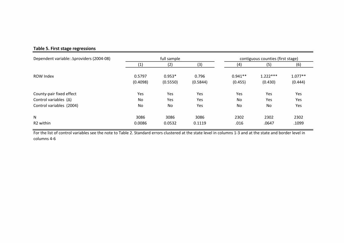
Table 5. First stage regressions

Dependent variable: providers (2004‐08) (1) (2) (3) (4) (5) (6)

ROW Index 0.5797 0.953* 0.796 0.941** 1.222*** 1.077**(0.4098) (0.5550) (0.5844) (0.455) (0.430) (0.444)

County‐pair fixed effect Yes Yes Yes Yes Yes YesControl variables  (Δ) No Yes Yes No Yes YesControl variables  (2004) No No Yes No No Yes

N 3086 3086 3086 2302 2302 2302R2 within 0.0086 0.0532 0.1119 .016 .0647 .1099

contiguous counties (first stage)full sample

For the list of control variables see the note to Table 2. Standard errors clustered at the state level in columns 1‐3 and at the state and border level in columns 4‐6

Table 6. Comparing the sample of bordering counties to the full sample of US counties

Full Sample (mean) Full Sample (sd) Bordering Counties

(mean)Bordering Counties

(sd) Difference (p-value)

unemployment % 5.66 (1.78) 5.65 (1.88) 0 0.95

young (18-29) voters % 15.68 (3.38) 15.17 (2.72) 0.51 0

population density (log) 2.83 (1.68) 2.66 (1.7) 0.17 0

black % 9 (14.36) 8.13 (13.67) 0.87 0.08

hispanic % 6.9 (12.32) 5.65 (8.86) 1.24 0

asian % 0.91 (1.79) 0.82 (1.67) 0.09 0.13

poverty % 13.77 (5.13) 13.67 (5.17) 0.1 0.58

mean income (log) 10.52 (0.23) 10.51 (0.24) 0.01 0.12

college educated % 17.69 (8.09) 17.15 (7.32) 0.54 0.05

male % 49.64 (2.02) 49.55 (1.7) 0.08 0.21

elderly (above 65) % 15.05 (4.11) 15.52 (4.12) -0.48 0

mean elevation 436.87 (498.03) 525.87 (564.27) -89 0

mean slope 2.12 (2.48) 2.67 (2.84) -0.54 0

elevation (sd) 74.56 (114.85) 95.49 (128.22) -20.92 0

Republican vote 2000 58.89 (12.13) 58.63 (12.76) 0.26 0.54

Republican vote 2004 60.97 (12.55) 60.82 (12.8) 0.15 0.73

turnout 2000 53.27 (9.01) 53.71 (8.87) -0.44 0.16

turnout 2004 58.52 (9.29) 58.69 (8.67) -0.16 0.6

The table reports the means and standard deviations of, respectively, the full sample of US counties used in the regressions and the sample of contiguous counties. When not otherwise specified, the value refers to the pre-treatment situation, i.e. 2004.

Table 7. Testing the similarity of bordering county pairs vs randomly paired counties

Full Sample (sd)

Bordering Counties (sd) Ratio p-value (one

sided)

unemployment % 0.927 1.263 0.73 0young voters % 1.897 2.375 0.8 0population density 0.622 1.172 0.53 0black % 4.21 10.323 0.41 0hispanic % 3.292 8.725 0.38 0asian % 0.752 1.272 0.59 0poverty % 2.331 3.706 0.63 0mean income 0.102 0.165 0.62 0college educated % 4.008 5.603 0.72 0male % 1.153 1.435 0.8 0elderly % 2.016 2.858 0.71 0mean elevation 80.999 359.881 0.23 0mean slope 0.731 1.77 0.41 0elevation (sd) 33.593 81.293 0.41 0Rep vote 2000 5.764 8.672 0.66 0Rep vote 2004 5.866 8.984 0.65 0turnout 2000 4.146 6.254 0.66 0turnout 2004 4.224 6.459 0.65 0Δ unemployment 0.654 0.889 0.74 0 Δ young voters 0.007 0.009 0.83 0Δ population density 0.027 0.04 0.68 0Δ black 0.003 0.005 0.72 0Δ hispanic 0.005 0.006 0.73 0Δ asian 0.001 0.001 0.91 0Δ poverty 0.011 0.014 0.8 0Δ income 0.033 0.042 0.78 0Δ college educated 0.007 0.008 0.92 0Δ male 0.002 0.003 0.81 0Δ elderly 0.672 0.497 1.35 1

The p-value refers to a one-sided F-test where the nul hypothesis is that the standard deviaton of the distribution of within-pair differences is smaller for bordering than for randomly paired counties. Baseline values refer to 2004, the Δ refers to changes between 2004 and 2008. Population density and mean county income are expressed in logs.

Table 8. Estimates using contiguous county pairs: Democratic party vote share, turnout and campaign contributions

(1) (2) (3) (4) (5) (6) (7) (8) (9) (10) (11) (12)

Providers 0.185** 0.197** 0.153** 0.107* 0.132** 0.144** 0.160*** 0.182*** 0.024 0.029 0.056 0.046(0.083) (0.081) (0.70) (0.064) (0.061) (0.062) (0.061) (0.057) (0.055) (0.058) (0.056) (0.057)

Control variables  (Δ) Yes Yes Yes Yes Yes Yes Yes Yes Yes Yes Yes Yes

Control variables  (2004) No Yes No Yes No Yes No Yes No Yes No Yes

N 2302 2302 2302 2302 2302 2302 2302 2302 2302 2302 2302 2302

R2 .070 .256 .114 .259 .019 .042 .0.24 .052 .014 .024 .020 .041

Small contr. R

For the list of control variables see the note to Table 2. Standard errors are double clustered at the state and border level. *** significant at 1% level, ** at 5%, * at 10% 

Vote share D Turnout Contributions D Small contr. D Contributions R

Table 9. IV estimates using contiguous county pairs: Democratic party vote share, turnout and campaign contributions

Providers 0.516 0.718 1.644** 1.648* ‐0.326 ‐0.240 ‐0.055 0.026 0.233 0.233 0.128 0.262

(0.914) (1.032) (0.820) (0.905) (0.482) (0.487) (0.464) (0.484) (0.365) (0.443) (0.324) (0.381)

Control variables (Δ) Yes Yes Yes Yes Yes Yes Yes Yes Yes Yes Yes Yes

Control variables (2004) No Yes No Yes No Yes No Yes No Yes No Yes

Cragg‐Donald F‐statistic 30.67 22.84 30.67 22.84 30.67 22.84 30.67 22.84 30.67 22.84 30.67 22.84

N 2302 2302 2302 2302 2302 2302 2302 2302 2302 2302 2302 2302

Small contr R

For a list of control variables see the note to Table 2. The Stock and Yogo (2005) 10% critical value  is 16.38. Standard errors are double clustered at the state and border level. *** significant at 1% level, ** at 5%, * at 10% 

Vote share D Turnout Contributions D Small contr D Contributions R

Table 10. IV Estimates: Heterogeneous Effects

Dep variable

(1) (2) (3) (4) (5) (6) (7) (8) (9) (10) (11) (12) (13) (14) (15)

Providers x Young ‐2.205 .859 2.179(1.747) (1.248) (1.712)

Providers x Black ‐1.156 .219  1.743*(1.257) (.581) (1.005)

Providers x College ‐.497 ‐.031 .41884(1.146) (.595) (1.408)

Providers x Income ‐.964 ‐.559 ‐1.335(.814) (.454) (1.203)

Providers x Density ‐.044 .015 .173*(.107) (.072) (.098)

Control variables  (Δ) Yes Yes Yes Yes Yes Yes Yes Yes Yes Yes Yes Yes

N 2302 2302 2302 2302 2302 2302 2302 2302 2302 2302 2302 2302

For the list of control variables see the note to Table 2. Standard errors are double clustered at the state and border level. *** significant at 1% level, 

Turnout Small Contributions D Democratic candidate vote share

Table 11. IV estimates using contiguous county pairs and excluding close races (margin < 5%)

(1) (2) (3) (4) (5) (6) (7) (8) (9) (10) (11) (12)

Providers 0.033 ‐0.119 1.730** 1.470* ‐0.732 ‐0.489 ‐0.517 ‐0.412 0.422 0.287 0.320 0.446

(0.950) (0.869) (0.812) (0.823) (0.730) (0.601) (0.701) (0.598) (0.483) (0.497) (0.478) (0.533)

Control variables (Δ)

Yes Yes Yes Yes Yes Yes Yes Yes Yes Yes Yes Yes

Control variables (2004)

No Yes No Yes No Yes No Yes No Yes No Yes

Cragg‐Donald      F‐stat

18.025 16.431 18.025 16.431 18.025 16.431 18.025 16.431 18.025 16.431 18.025 16.431

N 1612 1612 1612 1612 1612 1612 1612 1612 1612 1612 1612 1612

For a list of control variables see the note to Table 2. The Stock and Yogo (2005) 10% critical value  is 16.38. Standard errors are double clustered at the state and border level. *** significant at 1% level, ** at 5%, * at 10% 

Vote share D Turnout Contributions D Small contr D Contributions R Small contr R