The polygon overlay problem in electoral geography

Romain Louvet*1,2, Jagannath Aryal2, Didier Josselin1,3, Christele Marchand-Lagier4,Cyrille Genre-Grandpierre1

1UMR ESPACE 7300 CNRS, Universite d’Avignon, France2University of Tasmania, Discipline of Geography and Spatial Sciences, School of Land and Food

3LIA, Universite d’Avignon, France4CHERPA, Aix-en-Provence, LBNC, Universite d’Avignon, France

*Corresponding author: romain.louvet@alumni.univ-avignon.fr

AbstractWe developed an algorithm for reducing geometric differences between a source and a target

dataset. The algorithm tackles the polygon overlay problem in electoral geography before using

areal interpolation methods. Our results show that improvement in matching between statistical

areas and polling areas can reduce up to 40% of areal interpolation errors. This is applied to two

case studies: the city of Avignon, France, and the city of Hobart, Australia.

Keywordspolygon overlay problem, areal interpolation, spatial disaggregation, spatial aggregation, COSP

I INTRODUCTIONWhen we explain elections based on socio-spatial context, one main methodological issue is the

need to compare variables from different sources, i.e. electoral results with sociological and eco-

nomical variables. The areal units used for mapping these variables, being designed for different

purposes, usually come with different spatial resolutions and different boundaries.Therefore, it

is an issue when studying the relationship between variables or trying to compare data over time

(Fotheringham and Rogerson, 2013). This issue has been defined as one example of the Change

Of Support Problem (COSP) called the polygon overlay problem when dealing with incompat-

ible area to area spatial data (Gotway and Young, 2002). Being confronted with this problem,

it is necessary to reallocate data from a source dataset to a target dataset, or in other words

from the areal units with available data to the areal units of interest, by using areal interpolation

methods.

Areal interpolation is a widely known and studied problem in spatial science and encountered

with many type of data (Carson, 2013; Fotheringham and Rogerson, 2013). Many methods

already exist (Tobler, 1979; Mugglin et al., 1999; Eicher and Brewer, 2001; Mennis and Hult-

gren, 2006; Reibel and Agrawal, 2007; Krivoruchko et al., 2011; Zhang and Qiu, 2011; Qiu

et al., 2012; Lin et al., 2011), have been compared (Goodchild et al., 1993; Lam, 1983; Carson,

2013; Fotheringham and Rogerson, 2013; Do, 2015), and have been implemented. This paper

does not propose a new method of areal interpolation but a process to reduce areal interpolation

error by improving matching between source and target data.

Areal interpolation methods model spatial distribution based on strong assumptions such as

homogeneity, isotropy, and stationarity. These assumptions, more fitted to natural phenomenon,

1

Proceedings of Spatial Accuracy 2016 [ISBN: 978-2-9105-4510-5]

67 / 366

can fail to model human spatial distribution. Although intelligent and sophisticated methods

can improve greatly their fitness to the actual spatial distribution, they are still subjected of

generating interpolation errors. Therefore the polygon overlay problem is raising questions

about the actual accuracy of analyses of electoral behaviour in their spatial context.

Another less common approach to this problem would be trying to reduce the mismatch between

the source and target dataset. Such a method is based on aggregating algorithms which create

new areal units optimizing an objective. This idea of an automated zoning procedure (AZP)

was developed by Openshaw (1977) to solve the Modifiable Areal Unit Problem (MAUP) and

has been applied as a solution to the polygon overlay problem by Martin (2003). Creating

more fitted areal units could be indeed useful in the case of electoral geography because both

geometric and attributes accuracy of polling areas are actually questionable (Bernard et al.,

2015).

In this study, we combine areal interpolation with our algorithm, similar to AZP and sliver

polygons eliminating tools, in order to reduce first the differences between the source and target

dataset before using areal interpolation. Then it is expected that the results of areal interpolation

will have fewer errors. This idea was applied to two case studies, one in France, and the other

in Australia.

II MATERIAL AND METHODS

0 5 102.5 Kilometers

¯ ¯

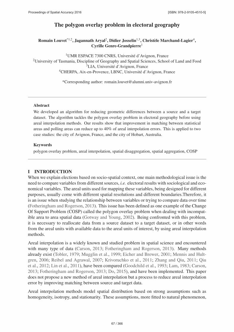
Figure 1: 2012 national election polling areas (left) and 2010 IRIS statistical areas (right), respectively

target and source data of the city of Avignon, France

2

Proceedings of Spatial Accuracy 2016 [ISBN: 978-2-9105-4510-5]

68 / 366

0 5 102.5 Kilometers

¯ ¯

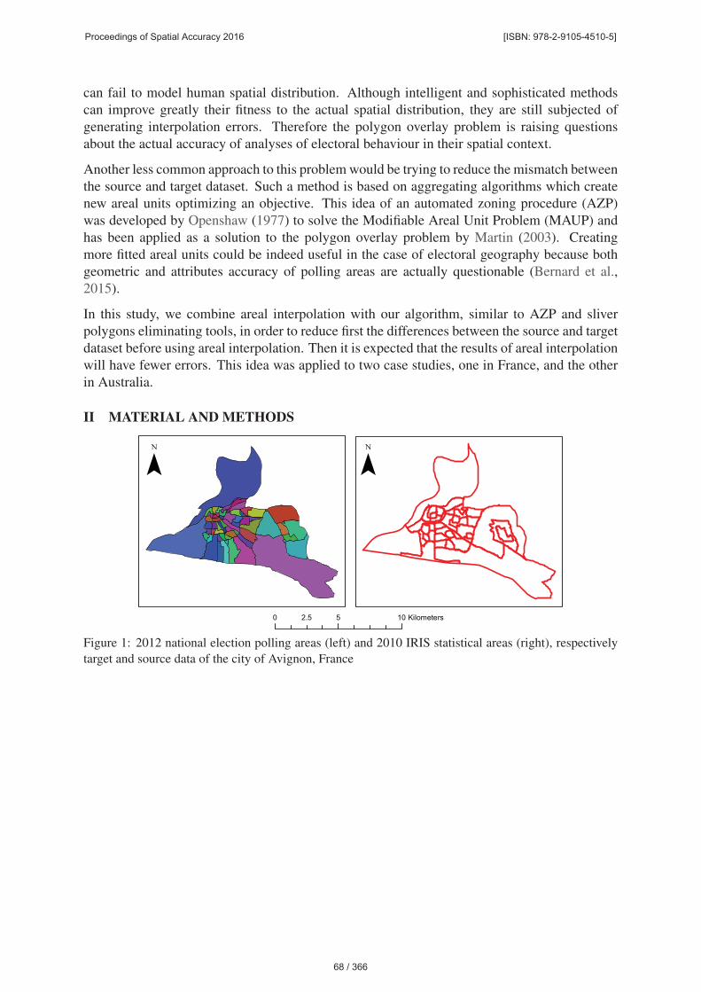
Figure 2: 2013 federal election polling areas (left) and 2011 SA1 statistical areas (right), respectively

target and source data of the city of Hobart, Australia

We are comparing two study areas with similar populations but different densities and polling

systems: Avignon (figure 1) and Hobart (figure 2).

We choose to use four areal interpolation methods, based on: area weighting, binary dasymetric,

Kriging, and Geographically Weighted Regression. As ancillary data, we used building areas

from land use for Avignon, and buildings polygons and points for Hobart. For both study areas,

we used the number of dwellings as explanatory variable.

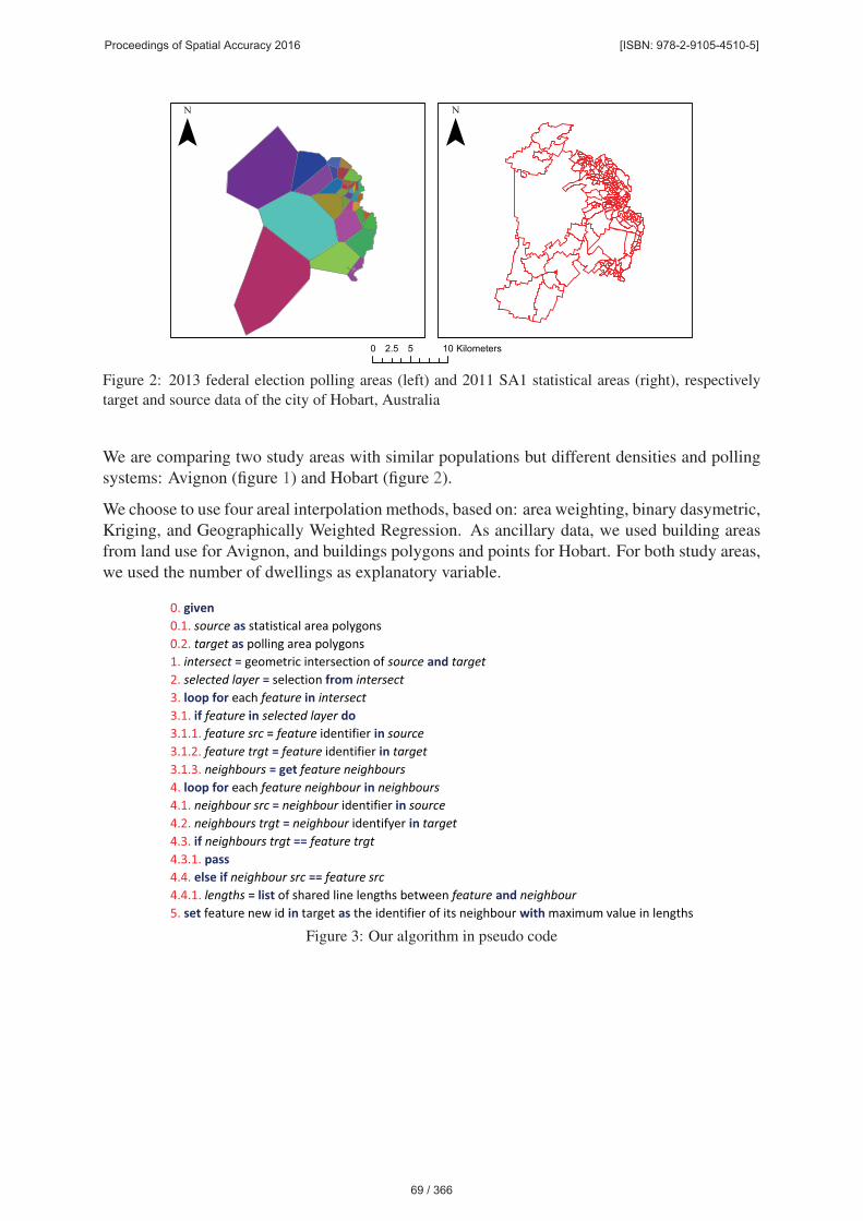
0. given0.1. source as statistical area polygons0.2. target as polling area polygons1. intersect = geometric intersection of source and target2. selected layer = selection from intersect3. loop for each feature in intersect3.1. if feature in selected layer do3.1.1. feature src = feature identifier in source3.1.2. feature trgt = feature identifier in target3.1.3. neighbours = get feature neighbours4. loop for each feature neighbour in neighbours4.1. neighbour src = neighbour identifier in source4.2. neighbours trgt = neighbour identifyer in target4.3. if neighbours trgt == feature trgt4.3.1. pass4.4. else if neighbour src == feature src4.4.1. lengths = list of shared line lengths between feature and neighbour5. set feature new id in target as the identifier of its neighbour with maximum value in lengths

Figure 3: Our algorithm in pseudo code

3

Proceedings of Spatial Accuracy 2016 [ISBN: 978-2-9105-4510-5]

69 / 366

1 2

3 4

¯0 500250 Meters

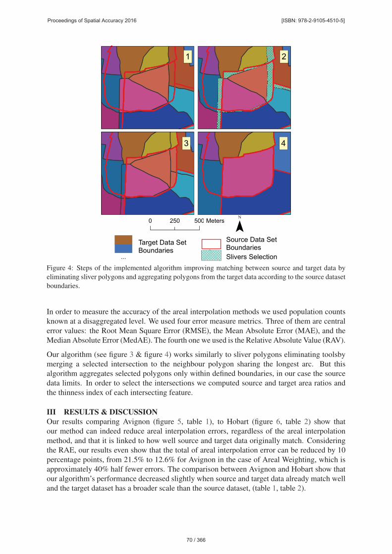
Source Data SetBoundariesSlivers Selection

Target Data SetBoundaries

...

Figure 4: Steps of the implemented algorithm improving matching between source and target data by

eliminating sliver polygons and aggregating polygons from the target data according to the source dataset

boundaries.

In order to measure the accuracy of the areal interpolation methods we used population counts

known at a disaggregated level. We used four error measure metrics. Three of them are central

error values: the Root Mean Square Error (RMSE), the Mean Absolute Error (MAE), and the

Median Absolute Error (MedAE). The fourth one we used is the Relative Absolute Value (RAV).

Our algorithm (see figure 3 & figure 4) works similarly to sliver polygons eliminating toolsby

merging a selected intersection to the neighbour polygon sharing the longest arc. But this

algorithm aggregates selected polygons only within defined boundaries, in our case the source

data limits. In order to select the intersections we computed source and target area ratios and

the thinness index of each intersecting feature.

III RESULTS & DISCUSSIONOur results comparing Avignon (figure 5, table 1), to Hobart (figure 6, table 2) show that

our method can indeed reduce areal interpolation errors, regardless of the areal interpolation

method, and that it is linked to how well source and target data originally match. Considering

the RAE, our results even show that the total of areal interpolation error can be reduced by 10

percentage points, from 21.5% to 12.6% for Avignon in the case of Areal Weighting, which is

approximately 40% half fewer errors. The comparison between Avignon and Hobart show that

our algorithm’s performance decreased slightly when source and target data already match well

and the target dataset has a broader scale than the source dataset, (table 1, table 2).

4

Proceedings of Spatial Accuracy 2016 [ISBN: 978-2-9105-4510-5]

70 / 366

0.0 0.1 0.2

GWR

Kriging

Dasymetric

Area

Normalized Root Mean Square Error

Original Target Data New Target Data

(a)

0.0 0.1 0.2

GWR

Kriging

Dasymetric

Area

Normalized Mean Absolute Error

Original Target Data New Target Data

(b)

0.0 0.1 0.2

GWR

Kriging

Dasymetric

Area

Normalized Median Absolute Error

Original Target Data New Target Data

(c)

0.0 0.1 0.2

GWR

Kriging

Dasymetric

Area

Relative Absolute Error

Original Target Data New Target Data

(d)

Figure 5: Avignon, Areal interpolation errors of population count, original polling areas and polling

areas modified by our algorithm

0.00 0.02 0.04 0.06 0.08 0.10

GWR

Kriging

Dasymetric

Area

Normalized Root Mean Square Error

Original Target Data New Target Data

(a)

0.00 0.02 0.04 0.06 0.08 0.10

GWR

Kriging

Dasymetric

Area

Normalized Mean Absolute Error

Original Target Data New Target Data

(b)

0.00 0.02 0.04 0.06 0.08 0.10

GWR

Kriging

Dasymetric

Area

Normalized Median Absolute Error

Original Target Data New Target Data

(c)

0.00 0.02 0.04 0.06 0.08 0.10

GWR

Kriging

Dasymetric

Area

Relative Absolute Error

Original Target Data New Target Data

(d)

Figure 6: Hobart, Areal interpolation errors of population count, original polling areas and polling areas

modified by our algorithm

5

Proceedings of Spatial Accuracy 2016 [ISBN: 978-2-9105-4510-5]

71 / 366

Polling Area Geometric PrecisionOriginal Target Data New Target Data Precision Variation (%)

Smallest Unit (ha) 7.9 9.3 -15

Number of Units 57 43 -25

Intersects with Statistical Area Geometric PrecisionOriginal Target Data New Target Data Precision Variation (%)

Smallest Unit (ha) 0.001 0.9 -99.9

Number of Units 281 94 -66

Interpolation Errors VariationRMSE MAE MedAE RAE

% people % people % people % people

Area Weighting -23 -101 -24 -85 -21 -66 -43 -8489

Binary Dasymetric -20 -86 -23 -75 -34 -90 -42 -7954

GWR +14 +50 +18 +48 +25 +56 -11 -1697

Kriging -17 -66 -27 -81 -47 -126 -45 -7714

Table 1: Avignon, geometric precision and interpolation errors, original target data and the new target

Polling Area Geometric PrecisionOriginal Target Data New Target Data Precision Variation (%)

Smallest Unit (ha) 2.3 36.3 -94

Number of Units 35 34 -3

Intersects with Statistical Area Geometric PrecisionOriginal Target Data New Target Data Precision Variation (%)

Smallest Unit (ha) 0.001 5 -99.998

Number of Units 415 238 -43

Interpolation Errors VariationRMSE MAE MedAE RAE

% people % people % people % people

Area Weighting -4 -9 -8 -13 -10 -10 -26 -1531

Binary Dasymetric -10 -13 -16 -17 -45 -43 -33 -1204

GWR -10 -17 -4 -5 +15 +12 -23 -1058

Kriging -2 -5 +1 +1 +21 +21 -20 -1022

Table 2: Hobart, geometric precision and interpolation errors, original target data and new target data

6

Proceedings of Spatial Accuracy 2016 [ISBN: 978-2-9105-4510-5]

72 / 366

ReferencesBernard L., Marchand-Lagier C., Josselin D., Louvet R. (2015, June). Some ways to estimate the effects of the

bad voters registration on electoral participation. In Congres AFSP 2015, Aix-en-Provence, France.

Carson B. D. (2013). Testing Kriging-Based Areal Interpolation for Census-Based Socioeconomic Data. Master’s

thesis, University of Redlands.

Do V. H. (2015). Les methodes d’interpolation pour donnees sur zones. Ph. D. thesis, Toulouse 1.

Eicher C. L., Brewer C. A. (2001). Dasymetric mapping and areal interpolation: Implementation and evaluation.

Cartography and Geographic Information Science 28(2), 125–138.

Fotheringham S., Rogerson P. (2013, April). Spatial Analysis And GIS. CRC Press.

Goodchild M. F., Anselin L., Deichmann U. (1993). A Framework for the Areal Interpolation of Socioeconomic

Data. Environment and Planning A 25, 383–397.

Gotway C. A., Young L. J. (2002). Combining incompatible spatial data. Journal of the American StatisticalAssociation 97(458), 632–648.

Krivoruchko K., Gribov A., Krause E. (2011). Multivariate Areal Interpolation for Continuous and Count Data.

Procedia Environmental Sciences 3, 14–19.

Lam N. S.-N. (1983, January). Spatial Interpolation Methods: A Review. The American Cartographer 10(2),

129–150.

Lin J., Cromley R., Zhang C. (2011, March). Using geographically weighted regression to solve the areal interpo-

lation problem. Annals of GIS 17(1), 1–14.

Martin D. (2003, March). Extending the automated zoning procedure to reconcile incompatible zoning systems.

International Journal of Geographical Information Science 17(2), 181–196.

Mennis J., Hultgren T. (2006). Intelligent dasymetric mapping and its application to areal interpolation. Cartog-raphy and Geographic Information Science 33(3), 179–194.

Mugglin A. S., Carlin B. P., Zhu L., Conlon E. (1999). Bayesian areal interpolation, estimation, and smoothing:

an inferential approach for geographic information systems. Environment and Planning A 31(8), 1337–1352.

Openshaw S. (1977). A Geographical Solution to Scale and Aggregation Problems in Region-Building, Partition-

ing and Spatial Modelling. Transactions of the Institute of British Geographers 2(4), 459–472.

Qiu F., Zhang C., Zhou Y. (2012, September). The Development of an Areal Interpolation ArcGIS Extension and

a Comparative Study. GIScience & Remote Sensing 49(5), 644–663.

Reibel M., Agrawal A. A. (2007). Areal interpolation of population counts using pre-classified land cover data.

Population Research and Policy Review, 10–1007.

Tobler W. R. (1979). Smooth pycnophylactic interpolation for geographical regions. Journal of the AmericanStatistical Association 74(367), 519–530.

Zhang C., Qiu F. (2011, March). A Point-Based Intelligent Approach to Areal Interpolation. The ProfessionalGeographer 63(2), 262–276.

7

Proceedings of Spatial Accuracy 2016 [ISBN: 978-2-9105-4510-5]

73 / 366