the popcycling-baltic model
TRANSCRIPT

NIL
U: O
R 10/2000
The POPCYCLING-Baltic Model
A Non-Steady State Multicompartment Mass Balance
Model of the Fate of Persistent Organic Pollutants in the Baltic Sea
Environment
Frank Wania1, Johan Persson2, Antonio Di Guardo3, Michael S. McLachlan4,
1 Norwegian Institute for Air Research, NILU 2 Institute of Applied Environmental Research (ITM), Stockholm University 3 Environmental Research Group, Department of Structural and Functional Biology, University of Insubria
4 IOW Baltic Sea Research Institute
NILU: OR 10/2000 REFERENCE U-96069 DATE: MARCH 2000 ISBN: 82-425-1159-4
The POPCYCLING-Baltic Model
NILU OR 10/2000
2
The POPCYCLING-Baltic Model A Non-Steady State Multicompartment Mass Balance Model of the Fate of
Persistent Organic Pollutants in the Baltic Sea Environment
Foreword and Acknowledgements The multimedia fate and transport model for the Baltic Sea environment which is described in this document was developed as part of the POPCYCLING-Baltic Project (contract No. ENV4-CT96-0214) of the Environment and Climate Research Programme of the European Union. This project, involving a collaboration of partners from Norway, Sweden, Finland, Denmark, Germany, Poland and Italy, was coordinated by Dr. Jozef M. Pacyna of the Norwegian Institute for Air Research (NILU).
In addition to the authors of this report, which were directly involved in the development of the model and its computer programme – Dr. Frank Wania from NILU, Johan Persson from Stockholm University, Dr. Antonio Di Guardo from the University of Insubria in Varese, Italy, and Dr. Michael S. McLachlan from the Baltic Sea Research Institute in Warnemünde, Germany – a great many people contributed in various ways to the progress of the model. Without Dr. Jozef Pacyna’s superiour coordination and organisation skills, the POPCYCLING-Baltic project would neither have come into existence, nor would it have been brought to a successful completion. David Henry of GRID Arendal, Norway supplied many of the spatially resolved environmental input data for the Baltic Sea drainage basin, Dr. Jesper Christensen from the National Environmental Research Institute (NERI) in Roskilde, Denmark derived the atmospheric advection rates using a Eulerian transport model, and Dr. Krzysztof Olendrzynski from the Norwegian Meteorological Institute (DNMI) supplied the remaining atmospheric input parameters. Drs. Seija Sinkkonen and Jaakko Paasivirta of the University of Jyväskylä, Finland were instrumental in deriving chemical input parameters. Knut Breivik from NILU, Dr. Dag Broman from Stockholm University, and Dr. Davide Calamari of the University of Insubria and the other participants in the POPCYCLING-Baltic project have readily shared their experience and knowledge in numerous discussions and work meetings. Their contributions to the POPYCLCING-Baltic are gratefully acknowledged.

The POPCYCLING-Baltic Model
NILU OR 10/2000
3

The POPCYCLING-Baltic Model
NILU OR 10/2000
4
Contents
Page
The POPCYCLING-Baltic Model.............. 2
A Non-Steady State Multicompartment Mass Balance Model of the Fate of Persistent Organic Pollutants in the Baltic Sea Environment ........................................................ 2
Foreword and Acknowledgements ..................................................................................... 2
Contents..................................................................................................................................... 4
1 Introduction and Motivation ................................................................................................ 9
1 Introduction and Motivation ................................................................................................ 9
1.1 Persistent Organic Pollutants in the Baltic Sea Environment........................................ 9
1.2 Motivation for Developing the POPCYCLING-Baltic Model .......................................... 9
2 System Boundary and Compartments of the POPCYCLING-Baltic Model ................. 11
2.1 The System Boundary................................................................................................ 11
2.2 Compartments in the POPCYCLING-Baltic Model ..................................................... 11
2.2.1 The Terrestrial Environment ................................................................................ 11
2.2.2 The Aquatic Environment .................................................................................... 13
2.2.3 The Atmospheric Environment............................................................................. 13
3 Description of the Natural Environment in the POPCYCLING Model ........................ 17
3.1 Mass Balances for Air, Water and Organic Carbon.................................................... 17
3.1.1 The Mass Balance for Air .................................................................................... 17
3.1.2 The Mass Balance for Water ............................................................................... 19
The Water Balance in the Terrestrial Environment.................................................... 19
The Water Balance in the Marine Environment......................................................... 23
3.1.3 The Mass Balance for Particulate Organic Carbon .............................................. 23
Other Organic Carbon fluxes .................................................................................... 29
3.2. Other Environmental Properties ................................................................................ 29
3.2.1 Temperatures ...................................................................................................... 29
3.2.2 Wind Speeds ....................................................................................................... 29
3.2.3 OH Radical Concentrations ................................................................................. 30
3.2.4 Forest Canopy Development ............................................................................... 31
Forest Volume and Composition ............................................................................... 31
Litter Fall ................................................................................................................... 32
3.2.5 Surface Cover and Soil Properties....................................................................... 33
3.2.6 Sediment Properties ............................................................................................ 33

The POPCYCLING-Baltic Model
NILU OR 10/2000
5
3.2.7 Atmospheric Parameters ..................................................................................... 33
4 Description of Contaminant Fate in the POPCYCLING-Model .................................... 34
4.1 Description of Phase Partitioning in the POPCYCLING-Baltic Model ......................... 34
4.1.1 Phase Partitioning in the Atmosphere.................................................................. 34
4.1.2 Phase Partitioning in the Aqueous Systems ........................................................ 35
4.1.3 Phase Partitioning in the Soil System .................................................................. 35
4.1.4 Z-value for the Forest Canopy ............................................................................. 35
4.2 Description of Chemical Processes in the POPCYCLING-Baltic Model...................... 36
4.2.1 Description of Advection Processes..................................................................... 36
Description of Atmospheric Advection....................................................................... 36
Description of Advection in Water ............................................................................. 36
Description of Soil-Fresh Water Exchange ............................................................... 36
Description of Sediment Burial .................................................................................. 36
Description of Litter Fall ............................................................................................ 37
4.2.2 Description of Air-Surface Exchange ................................................................... 37
Description of Dry Particle Deposition ....................................................................... 37
Description of Wet Deposition................................................................................... 39
Description of Diffusive Air-Water Exchange ............................................................ 39
Description of Air-Forest Canopy-Forest Soil Exchange ........................................... 40
Description of Diffusive Air-Soil Exchange ................................................................ 40
4.2.3 Description of Water-Sediment Exchange ........................................................... 42
4.2.4 Description of Degradation Processes................................................................. 42
Description of Atmospheric Degradation ................................................................... 42
Degradation in Other Media ...................................................................................... 42
4.2.5 Description of Emissions and Boundary Conditions in the POPCYCLING model 43
Calculating Compartmental Release Rates from National Release Estimates .......... 43
Mode of Release and Seasonality............................................................................. 43
Boundary Conditions................................................................................................. 44
4.3 The Mass Balance Equations..................................................................................... 46
4.3.1 The Mass Balance Equations .............................................................................. 46
4.3.2 The Solution of the Mass Balance Equations....................................................... 46
5. References............................................................................................................................ 48
Appendix 1: Glossary ............................................................................................................. 52
Environmental Properties................................................................................................. 52
Compartment dimensions............................................................................................. 52
Volume fractions in m3/m3............................................................................................. 52
Transport Parameters................................................................................................... 52

The POPCYCLING-Baltic Model
NILU OR 10/2000
6
Mass transfer coefficients in m/h .................................................................................. 52
Diffusivities in m2/h ....................................................................................................... 53
wGXY water advection rates from compartment X to compartment Y in units of m3/h.... 53
oGX flux or rate of POC within aquatic system X in units of m3 POC/h .................... 53
Other advective transfer rates in m3/h .......................................................................... 53
Chemical Properties......................................................................................................... 53
Z-values in mol/(m3· Pa)............................................................................................... 54
D-Values in units of mol/(h· Pa) ................................................................................... 54
Appendix 2: Mass Balance Equations .................................................................................. 55
Atmospheric Compartments............................................................................................. 55
Coastal Water Compartments.......................................................................................... 55
Open Water Compartments ............................................................................................. 56
Forest Canopy Compartments ......................................................................................... 57
Forest Soil Compartments ............................................................................................... 57
Agricultural Soil Compartments........................................................................................ 57
Fresh Water Compartments............................................................................................. 57
Fresh Water Sediment Compartments............................................................................. 58
Coastal Sediment Compartments .................................................................................... 58
Deep Sediment Compartments ........................................................................................ 58
Appendix 3: List of Figures ................................................................................................... 59
Appendix 4: List of Tables..................................................................................................... 60
Appendix 5: Description of the Computer Programme...................................................... 61
Table of Contents of Appendix 5 ...................................................................................... 61
Introduction ...................................................................................................................... 62
Set-up and Getting Started .............................................................................................. 62
Selecting and Displaying Environmental Input Parameters .............................................. 62
Editing Environmental Input Parameters....................................................................... 63
Time-Invariant Input parameters ............................................................................... 63
Time-Variant Input Parameters ................................................................................. 63
Returning Environmental Input Parameters to their Default Value................................ 64
Displaying Environmental Parameters in Tables, Time Graphs and Mass Balance Graphs ......................................................................................................................... 64
Displaying Some Atmospheric Parameters ............................................................... 64
Displaying Some Marine Parameters ........................................................................ 64
Displaying Some Terrestrial Parameters................................................................... 64
Displaying the Water Balance ................................................................................... 64
Displaying the POC Balance ..................................................................................... 65

The POPCYCLING-Baltic Model
NILU OR 10/2000
7
Displaying Time-Variant Environmental Parameters ................................................. 65
Selecting and Displaying Chemical Parameters............................................................... 65
Selecting Chemical Parameters.................................................................................... 65
Displaying Chemical Parameters.................................................................................. 66
Performing a Simulation................................................................................................... 66
Specifying a Emission Scenario and Boundary Conditions ........................................... 66
Reading File with Annual National Emission Rates and Boundary Conditions .......... 66
Specifying Other Parameters Related to the Emission Scenario............................... 67
Specifying the Simulation Conditions and Performing the Simulations ......................... 67
Displaying Model Results ................................................................................................. 68
Displaying the Simulation Results in Tables ................................................................. 69
Displaying the Simulation Results as Time Graphs ..................................................... 69
Displaying Fluxes in Overview Graphs.......................................................................... 69
Displaying Fluxes in the Terrestrial/Coastal Systems ................................................... 69
Displaying Graphs With Atmospheric, Marine and Terrestrial Results .......................... 69
Writing Results to File .................................................................................................. 69

The POPCYCLING-Baltic Model
NILU OR 10/2000
8

The POPCYCLING-Baltic Model
NILU OR 10/2000
9
1 Introduction and Motivation
1.1 Persistent Organic Pollutants in the Baltic Sea Environment
The Baltic Sea is a large, semi-enclosed brackish body of water in the North of Europe. Its drainage basin (Figure 1), which takes up the greater part of Northern Europe, covers an area of more than 2 million square kilometers, more than 20 % of which is taken up by water. It extends over 20 degrees of latitude (approx. 50 to 70 °N), and includes parts of fourteen countries (Sweden, Finland, Estonia, Latvia, Lithuania, Russia, Belorus, Poland, Germany, Denmark, Norway, the Czech and Slovak Republics, Ukraine). Because of its proximity and downwind location to the highly industrialised and densely populated areas of central Europe the Baltic Sea environment has been the recipient of airborne and riverine pollutants, including nutrients, acid rain and persistent organic pollutants. The latter have achieved particularly high concentrations in the Baltic Sea, and it was here that PCBs were first detected in environmental samples (Jensen et al., 1969). Seals and fish from the Baltic Sea are believed to be affected by the presence of these contaminants (Bengtsson et al. 1999; Olsson et al. 1992).
The Baltic Sea shares some characteristics with the Laurentian Great Lakes of North America, namely the climate and the proximity to sources of pollution, and similarly high levels of POPs were observed. Whereas, however the fate of POPs in the Great Lakes has been described in numerous studies with the help of mass balance models (Bierman and Swain, 1982; Thomann and DiToro, 1983; Sonzogni et al., 1987; Mackay, 1989; Bierman et al., 1992; Diamond et al., 1994; Mackay et al., 1994; Gobas et al., 1995), almost no such studies exist for the Baltic Sea (Wulff et al., 1993; Wania et al., 1999). Mass balance models help to obtain the “big picture” of a chemical’s behaviour in a regional environment. Their primary use is to simulate the observed behaviour of contaminants in a region. A successful simulation, i.e. comparability of observations and simulation results, suggests that the degree of theoretical understanding of the way chemicals partition, move and react is sufficient to explain the observed behaviour in the environment. It is then possible to further use the model to derive information not contained in the measured data, such as trend predictions, source apportionment and mass budgets (Wania and Mackay, 1999).
The POPCYCLING-Baltic project set out to develop a non-steady state multi-media mass balance model for describing the long term fate of persistent organic pollutants (POPs) in the Baltic Sea environment, building upon the earlier work by Wania et al. (1999). This report gives a detailed description of the POPCYCLING-Baltic model.
1.2 Motivation for Developing the POPCYCLING-Baltic Model
The POPCYCLING-Baltic model aims to distinguish and quantify the environmental path-ways of selected POPs in the Baltic Sea environment (Figure 2). In particular, it aims to estimate the fractions of the POPs currently present in various parts of that environment, which are derived from (i) recent releases within the drainage basin, (ii) past emissions in the drainage basin and (iii) contaminanted air masses being advected into the area. Within the model region, a main focus is on the relative importance of the riverine and atmospheric pathway for delivering POPs to the marine ecosystem of the Baltic Sea. Furthermore, the model is expected to address the question, what fraction of the riverine load is actually atmospherically derived vs. being emitted directly to the soils, plants and rivers of a drainage basin (Figure 2).
The description of the terrestrial part of the drainage basin of the Baltic Sea is restricted to those aspects which influence the magnitude and the timing of POPs delivery to the Baltic Sea. This implies that the model aims to describe accurately the rates of release (and the seasonal change of this release) of POPs from the main terrestrial storage media for POPs, i.e. soil and vegetation, into the two transport media delivering POPs to the marine

The POPCYCLING-Baltic Model
NILU OR 10/2000
10
environment, i.e. atmosphere and fresh water. Vegetation and soil have to be treated separately, if their characteristics of exchange with the atmosphere are different. This is the case for forests which display much faster uptake for many POPs than grassland and fields planted with agricultural crops (McLachlan and Horstmann, 1999).
Key processes are the two-directional exchange, or cycling, of POPs between the atmosphere and aquatic and terrestrial surfaces, and the uni-directional run-off of chemical from soil to fresh water and further to the marine system. Important are further the processes that could lead to loss of chemical during the transport in atmosphere and river water, i.e. degradation and deposition in the atmosphere, and degradation, net sedimenta-tion to fresh water sediments, and volatilisation in the fresh water system.
Figure 1 The drainage basin of the Baltic Sea (modified from GRID Arendal website: http://www.grida.no). (This figure does not include the Skagerrak region, even though it is included in the model).

The POPCYCLING-Baltic Model
NILU OR 10/2000
11
2 System Boundary and Compartments of the POPCYCLING-Baltic Model
2.1 The System Boundary
The modelled system comprises the entire drainage basin of the Baltic Sea, including the Kattegat and Skagerrak area (Figure 1). It also includes the troposphere above this drainage basin. This is a deviation from most previous models of contaminants in large water bodies which tend to be restricted to the aquatic environment. In aquatic models the air-water interface and the river mouths constitute system boundaries and riverine inflow concentrations and atmospheric concentrations over the water surface are model boundary conditions supplied by the user (Figure 3).
Such a model design neglects the possibility of interactions between the lake, the atmosphere above it and its drainage basin. It is well established that atmospheric concentrations of many POPs are governed by the exchange with the Earth’s surface, and it is conceivable that a large water body can act as a supply of persistent chemicals to its terrestrial surroundings and vice versa. Atmospheric and riverine concentrations therefore should be calculated by the model rather than being supplied as input parameters. This aspect of the model reflects a trend within water quality modelling to progressively include more parts of the overall system within the system boundaries (Thomann, 1998).
2.2 Compartments in the POPCYCLING-Baltic Model
A typical multi-media mass balance model divides the environment into a number of boxes or compartments, which are considered well-mixed and homogeneous, both with respect to the environmental characteristics and chemical contamination. These environmental phases are then linked by a variety of intercompartmental transfer processes (Cowan et al., 1995, Wania and Mackay, 1999). The POPCYCLING-Baltic model consists of 85 such boxes or compartments (Table 1). The division of the Baltic Sea environment into compartments was based on the following considerations:
• the units can be identified in physical geographical terms (e.g. water sheds).
• the units can be considered well mixed with respect to the time scales relevant for POPs.
• the units have similar characteristics with respect to environmental properties and emission rates of POPs.
The basic geographic units in the model are the eight aquatic sub-basins of the Baltic Sea and their respective drainage basins, namely:
Bothnian Bay Bothnian Sea Gulf of Finland Gulf of Riga Baltic Proper Danish Straits Kattegat Skagerrak
2.2.1 The Terrestrial Environment
The drainage basin of each of these sub-basins is represented in the model by a terrestrial unit. Because of their heterogeneity, the drainage basins of two aquatic sub-basins are represented by two terrestrial entities. In the Gulf of Finland, the model distinguishes the area drained by the River Neva from the remainder of the drainage basin, because of very different hydrological characteristics. In the Baltic Proper, the Swedish part and the Southern part of the drainage basin are treated separately, because of large differences in hydrology, climate, and emissions. Each of the ten terrestrial units (Figure 4A) is described by five compartments (agricultural soil, forest soil, forest canopy, fresh water, fresh water sediment).

The POPCYCLING-Baltic Model
NILU OR 10/2000
12
Model Region
advectiveinflow
lossloss
sourcessources
evaporationevaporationdepositiondeposition
advectiveoutflow
lossloss
AtmosphereAtmosphere
Marine SystemMarine System
evaporationevaporationdepositiondeposition
Terrestrial SystemTerrestrial System
lossloss
run-offrun-off
Figure 2 The POPCYCLING-Baltic model aims to quantify the pathways of POPs from the terrestrial environment to the marine environment via atmosphere and rivers.
aquatic model catchment modelWater
Atmosphere
��������������������������������������������������������������������������������������������������������������������������������������������������������������������������������������������������������������������������������������������������������������������������������������������������������������������������������������������������������������
Vegetation
Water
FreshWater
Sediment
Soil
Sediment
system boundary
Figure 3 The system of a catchment model includes the drainage basin of the water body and the atmosphere above it.

The POPCYCLING-Baltic Model
NILU OR 10/2000
13
2.2.2 The Aquatic Environment
A coastal unit, consisting of a water and a sediment compartment, is associated with each of the ten drainage basins. In the Gulf of Riga, the Danish Straits and the Kattegat, this coastal unit represents the entire aquatic subbasin, whereas in the remaining five aquatic subbasins there are additional open water units, again consisting of a water and a sediment compartment. In the case of the Baltic Proper, the open water unit is subdivided vertically into a surface and bottom water compartment. The boundary between coastal and open water units is the 20 m depth contour. The marine environment of the Baltic Sea is thus represented by 16 water and 15 sediment compartments (Figure 4B). The surface area of the marine water compartments and their average depth (Figure 10) were supplied by D. Henry of GRID Arendal.
2.2.3 The Atmospheric Environment
Reflecting the greater mobility of the atmosphere, there are only four atmospheric compartments covering the area of the drainage basin (Figure 4C). Each of these four compartments is characterised by a relatively homogeneous emission situation, which is usually determined by population density, extent of agricultural and industrial activity and the political-economic framework. The Northern air compartment (A1) comprises the Bothnian Bay and Sea area, the Eastern air compartment (A2) extends over the drainage basins of the Gulfs of Finland and Riga, the Southern air compartment (A3) covers the terrestrial unit to the South of the Baltic Proper and the Eastern half of the aquatic Baltic Proper. The Western air compartment (A4) finally includes the Swedish Baltic Proper, the Danish Straits, the Kattegat and Skagerrak.
In socio-economic terms, A1 represent “Northern Scandinavia” with low population density, low agricultural activity and few localised industries, A2 comprises the part of the Baltic Sea drainage basin belonging to the “former Soviet Union” with intermediate population density, industrial and agricultural activity, A3 comprises “central eastern Europe” with high population density, industrial and agricultural activity, and A4 represents “Southern Scandinavia” with intermediate population density, industrial and agricultural activity.
Figure 4 shows all the compartment types and how they are interconnected. It also indicates into which types of compartment chemical can be released and in which compartments degradation can be assumed to occur.
The following indices are used to denote the various types of compartments:
A atmospheric compartments T terrestrial units (comprising F, B ,E, W, and S) F forest canopy compartments B forest soil compartments E agricultural soil compartments W fresh water compartments S fresh water sediment compartments C coastal water compartments L coastal sediment compartments O open water compartments M deep sediment compartments

The POPCYCLING-Baltic Model
NILU OR 10/2000
14
Table 1 The subdivision of the Baltic Sea drainage basin into environmental compartments.
Geographic Entity
Terrestrial Region Coastal Region Marine Region Atmospheric Region
Bothnian Bay T1 Bothnian Bay C1 Bothnian Bay O1 Bothnian Bay A1 North
Bothnian Sea T2 Bothnian Sea C2 Bothnian Sea O2 Bothnian Sea A1 North
Gulf of Finland T3 Gulf of Finland C3 Gulf of Finland O3 Gulf of Finland A2 East
T4 Neva C4 Neva A2 East
Gulf of Riga T5 Gulf of Riga C5 Gulf of Riga A2 East
Baltic Proper T6 Southern Baltic Coast C6 Southern Baltic Coast A3 South
T7 Swedish Baltic Coast C7 Swedish Baltic Coast A4 West
O4 Baltic Proper A3 and A4
O5 Bottom Water -
Danish Straits T8 Danish Straits C8 Danish Straits - A4 West
Kattegat T9 Kattegat C9 Kattegat - A4 West
Skagerrak T10 Skagerrak C10 Skagerrak O6 Skagerrak A4 West
85 compartments 10 agricultural soil
10 forest soil
10 forest canopy
10 fresh water
10 fresh water sediment
10 coastal water
10 coastal sediment
6 open water
5 deep sediment
4 atmosphere

The POPCYCLING-Baltic Model
NILU OR 10/2000
15
T1 Bothnian Bay
T2 Bothnian Sea
T4 Neva
T3 Gulf of Finland
T5 Gulf of
Riga
T6 Southern
Baltic Proper
T7 Swedish
Baltic Proper
T8 Danish Straits
T9 Kattegat
T10 Skagerrak
C1 Coastal
Bothnian Bay
C2 Coastal
Bothnian Sea C4
Neva
C3 Coastal Gulf of Finland
C5 Gulf of
Riga
C6 Southern
Baltic Proper
C7 Swedish
Baltic Proper
C8 Danish Straits
C9 Kattegat
C10 Coastal
Skagerrak
O1 Open
Bothnian Bay
O2 Open
Bothnian Sea
O3 Open
Gulf of Finland
O6 Open
Skagerrak O4 OpenBaltic Proper
O5Bottom
water
A1 North
A2 East
A3 South
A4 West
Figure 4 Maps showing the compartmentalisation of the terrestrial (A), marine (B) and atmospheric (C) environment of the Baltic Sea drainage basin in the POPCYCLING-Baltic model. Each of the ten terrestrial units is represented by five compartment (agricultural soil, forest soil, forest canopy, fresh water, fresh water sediment), each of the marine units by a water and a sediment compartment.

The POPCYCLING-Baltic Model
NILU OR 10/2000
16
agriculturalagriculturalsoilsoil
forestforestsoilsoil
forestforestcanopycanopy
fresh waterfresh water
coastalcoastalsedimentsediment
coastalcoastalwaterwater
open open waterwater
bottombottomwaterwater
bottombottomsedimentsediment
atmosphere
interphase transferdirect emissiondegradation lossadvection with air and water
Terrestrial Environment Marine Environment
fresh water sedimentfresh water sediment
Figure 5 Schematic representation of the types of environmental compartments in the POPCYCLING-Baltic model and how they are connected by diffusive and advective transport terms. A chemical can be released into six types of compartments, and degradation can occur in all types of media.

The POPCYCLING-Baltic Model
NILU OR 10/2000
17
3 Description of the Natural Environment in the POPCYCLING Model
3.1 Mass Balances for Air, Water and Organic Carbon
The movement of persistent organic contaminants in the environment is closely associated with the movement of air, water and particulate organic carbon (POC). In the POPCYCLING-Baltic model advective intercompartmental transfer fluxes for the contaminants are calculated as the product of a flux of a carrier phase, namely air, water and POC (in units of volume per time) and a contaminant concentration in that phase (in units of moles per volume). Solving the mass balance for the contaminants thus requires the construction of mass balances for air, water and POC within the modelled system. This task is made more complex by the interdependence of the mass balances (Figure 6). For example, POC itself is advected with water and the POC balance is thus dependent on the water balance. It should be noted that the intercompartmental transfer of water between the atmospheric compartments (in the form of clouds etc.) is ignored in the model.
3.1.1 The Mass Balance for Air
The only compartments involved in the construction of a mass balance for air, are the four atmospheric compartments. Sixteen atmospheric advection rates are required: eight rates describing the exchange between the four air compartments and eight rates for the exchange with the world outside the model region (Figure 7).
These rates were derived using a three dimensional gridded air dispersion model for the EMEP region (Dr. Jesper Christensen, Department of Atmospheric Environment, National Environmental Research Institute, Roskilde, Denmark). The model was used to calculate the intercompartmental air fluxes (in units of m2/s) every six hours during the time period 1989-1996. These data were averaged across all eight years to yield long term average monthly mean fluxes in m2/h. Averaging for individual years had shown that the interannual variability of these monthly averages is relatively minor. The resulting monthly fluxes were not mass conserving and had to be slightly adjusted by hand to fulfill the mass balance on air (Tables 2 and 3 gives the corrected values). In the model the rates are multiplied with the user-specifiable atmospheric height to yield volume fluxes of m3 air/h.
The data clearly show the westward movement of air across the drainage basin, i.e. the eastbound fluxes tend to be higher than those directed towards the west. Meridional exchange, i.e. air transport in the North-South direction tends to be more balanced. The rates also show a clear seasonal dependence with lower fluxes in summer and higher values in winter. When expressed as air residence times in the four atmospheric compartments, the magnitude of that fluctuation is about a factor of two, i.e. residence times are approx. 30 hours in summer and 15 hours in winter (Figure 8). A closer look at the seasonality of these atmospheric advection rates shows, that it is mostly the higher, i.e. west bound fluxes that have a high seasonality, whereas the eastbound fluxes tend to be stable throughout the year. This is presumably an indication that the higher rates in winter are driven by winter storms that tend to come from the Atlantic Ocean.

The POPCYCLING-Baltic Model
NILU OR 10/2000
18
Water Mass Balance
POC Mass Balance
Contaminant Mass Balance
Air Mass Balance
Figure 6 Solving the mass balance for a POP requires the construction of mass
balances for air, water and particulate organic carbon (POC).
North
East
South
WestO to W
W to O
E to O
O to E
O to N N to O
E to N N to E
W to S
S to W
O to S S to O
W to N
N to W
S to EE to S
Figure 7 Sixteen atmospheric advection rates are used to describe the movement of air across the Baltic Sea drainage basin in the POPCYCLING-Baltic model (O stands for “outside of the model system”).

The POPCYCLING-Baltic Model
NILU OR 10/2000
19
0
5
10
15
20
25
30
35
0 50 100 150 200 250 300 350
Julian Day
air
resi
den
ce t
ime
in h
ou
rsWest
EastSouth
North
Figure 8 Seasonal variability of the residence time of air in the four atmospheric
compartments of the POPCYCLING model. The residence time is lower in the Western air compartment because of its smaller size.
3.1.2 The Mass Balance for Water
Water moves between all model compartments and the water balance is thus quite complex. The water balance in the terrestrial and marine environment are described separately, but they are of course linked by the riverine flow.
THE WATER BALANCE IN THE TERRESTRIAL ENVIRONMENT
Long term average rain rates over the various drainage basins were estimated based on a variety of sources (Norwegian Meteorological Institute (DNMI), Atlases). The long term average riverine inflow of water to the sub-basins of the Baltic Sea has been reported by HELCOM (1996) and Bergström and Carlsson (1994). For the Skagerrak such information is available from Fonselius (1991). The data are listed in Table 4.
The water input was allocated to the forest canopy, the agricultural soil and the fresh water compartments based on their relative surface coverage. It was assumed that all water is intercepted by the forest canopy, and no rain falls directly to the forest soil. With the input and output of water well established, the evaporation loss, i.e. the difference between the two, remained to be allocated to the various surfaces, in order to derive the water fluxes between the compartments. This was done by estimating the fraction of the total water flow to a compartment (forest canopy, forest soil, agricultural soil, fresh water) that evaporates from that compartment. For each drainage basin these fraction were adjusted until the calculated riverine inflow wGWC agreed with the literature values reported in Table 4. Table 5 gives the water flows used in the model simulations between the terrestrial compartments in units of km3/a. Figure 9 serves as a legend to this table.
Though these numbers may not be exact representations of the long term water balance in the various drainage basin, it is believed that they catch the essential characteristics and differences, such as the relatively high rain input in the western basins, the lower evaporation loss in the northern areas, or the greater potential for evaporation in the drainage basin of the Neva and the Southern Baltic region. At present the water fluxes are assumed constant in time, i.e. the model neglects the seasonality of precipitation input, evaporation intensity and riverine run-off.

The POPCYCLING-Baltic Model
NILU OR 10/2000
20
Table 2 Monthly mean rates of air movement aGXY between the four air compartments in units of 1010 m2/h.
N to E E to N E to S S to E S to W W to S W to N N to W
Jan 36.4 8.1 11.6 44.4 12.0 62.9 36.3 11.3
Feb 31.1 10.7 8.5 36.8 15.4 49.8 30.6 13.9
Mar 21.4 12.0 6.4 36.2 16.2 45.3 33.4 10.5
Apr 13.2 14.3 9.5 18.3 19.7 21.4 25.4 12.9
May 18.4 7.5 12.4 16.6 13.1 24.7 17.5 11.9
Jun 14.6 7.5 7.1 18.1 7.4 29.3 18.1 9.8
Jul 16.6 6.9 9.1 19.5 5.9 29.5 18.5 9.8
Aug 13.8 8.5 5.7 21.2 9.7 28.0 20.1 9.0
Sep 16.8 11.2 8.4 20.6 15.1 26.2 19.1 15.3
Oct 29.0 7.7 6.8 34.5 14.8 35.3 30.0 11.1
Nov 23.0 12.9 6.3 37.5 16.5 39.1 27.9 14.6
Dec 33.5 8.2 6.6 37.6 12.5 46.1 33.7 14.4
Annual 22.3 9.6 8.2 28.4 13.2 36.5 25.9 12.0
Table 3 Monthly mean rates of air movement between the four air compartments and the outside world (O) in units of 1010 m2/h.
N to O O to N E to O O to E S to O O to S W to O O to W
Jan 48.8 52.0 71.6 10.5 45.7 27.5 18.1 94.1
Feb 46.5 50.2 65.9 17.1 35.8 29.7 26.6 77.7
Mar 49.9 36.4 57.4 18.1 29.2 29.9 21.6 73.6
Apr 43.1 29.6 32.4 24.7 21.4 28.6 27.4 41.6
May 27.7 33.0 30.2 15.0 26.0 18.6 20.0 37.2
Jun 30.0 28.7 31.3 13.2 27.9 16.9 13.2 43.5
Jul 27.2 28.3 31.5 11.3 26.0 12.7 10.4 42.7
Aug 30.8 25.0 34.2 13.5 21.9 19.1 14.0 43.5
Sep 32.0 33.8 38.9 21.1 25.7 26.7 26.8 41.6
Oct 40.5 43.0 61.4 12.3 28.0 35.2 20.8 60.1
Nov 44.3 41.1 59.4 18.0 28.3 36.9 23.4 59.4
Dec 46.9 52.8 68.6 12.4 35.4 32.8 21.0 73.9
Annual 39.0 37.8 48.6 15.6 29.3 26.2 20.3 57.4

The POPCYCLING-Baltic Model
NILU OR 10/2000
21
Table 4 Annual average rain rate in the ten drainage basins in cm and riverine water flow to the Baltic Sea in km3 as reported by various studies.
T1 T2 T3 T4 T5 T6 T7 T8 T9 T10
rain rate cm/a 59 61 63 61 58 62 61 60 73 130
river flow km3/a (1) 98 95 114 29 100 8 29 71
river flow km3/a (2) 98 91 112 32 114 37
(1) HELCOM, 1986, except T10: Fonselius, 1991, (2) Bergström and Carlsson, 1994
atmosphere
agriculturalsoil
forestsoil
forestcanopy
fresh water
wGFAwGAF
wGFB
wGEAwGAE
wGBA
wGBW wGEW
wGWC
wGWAwGAW
Water Balance in the Terrestrial Environment
wGAF precipitation to canopywGFA evaporation from canopywGFB throughfall/stem flowwGBA evaporation from forest soilwGBW run-off/leaching from forest soilwGAE precipitation to agricultural soilwGEA evaporation from agricultural soilwGBW run-off/leaching from agricultural soilwGAW precipitation to fresh waterwGWA evaporation from fresh waterwGWC riverine run-off
Figure 9 Water fluxes between the compartments of a drainage basin.
Table 5 Annual average water fluxes between the compartments of the ten drainage basins in units of km3.
wGAF wGFA wGFB wGBA wGB
W wGAE wGEA wGEW wGAW wGWA wGW
C
T1 113 28.2 84.5 13.5 71.0 41.5 10.4 31.1 6.9 10.9 98.1
T2 90.5 18.1 72.4 8.0 64.4 42.4 8.5 33.9 7.3 10.6 95.1
T3 47.9 21.6 26.4 7.9 18.5 34.7 17.4 17.4 7.0 6.4 36.4
T4 88.5 37.2 51.3 15.4 35.9 67.1 33.5 33.5 27.3 19.3 77.4
T5 30.0 15.0 15.0 5.3 9.8 48.1 24.1 24.1 1.5 5.3 30.0
T6 69.4 38.2 31.2 12.5 18.7 228 137 91 3.4 22.6 90.5
T7 28.1 14.1 14.1 4.9 9.1 13.7 6.9 6.9 4.0 3.0 17.0
T8 1.2 0.5 0.7 0.1 0.6 14.8 6.6 8.1 0.4 0.9 8.1
T9 32.2 12.9 19.3 3.9 15.4 22.3 10.0 12.3 6.2 5.1 28.8
T10 57.4 20.1 37.3 7.5 29.9 69.1 25.6 43.6 5.3 7.9 70.8

The POPCYCLING-Baltic Model
NILU OR 10/2000
22
O156 m
24.5·10³ km²1371 km3
462 days
O2 73 m
62·10³ km²4528 km3
1084 days
O344 m
18.6·10³ km²820 km3
369 days
C5Gulf of Riga
22.7 m16.4·10³ km²
372 km3
2025 days
O5Bottom Water
38 m177·10³ km²
6722 km3
1668 days
14711000
249457
104207
139
255
37
67
510
Index Sub-Basinaverage depthsurface areawater volumeresidence time evaporation
precipitationriverine inflow
interbasin flow
2533
911
10
1130
1414
942
C25.8 m
22.9·10³ km²133 km3
46 days
964
106012
1395
C18.3 m
15·10³ km²125 km³47 days
876
9757
898
C7 Swedish Coast
7.9 m20.7·10³ km²
163 km3
45 days
1314
133212
1317
471
471
O4 Surface Water
30 m177·10³ km²
5307 km3
305 days
C6 Southern Coast
8.7 m32.2·10³ km²
280 km3
45 days16
1891
22822190
C35.7 m
11.6·10³ km²66 km3
43 days
526563
6
736
C4Neva1.0 m
0.3·10³ km²0.3 km3
1 day
108
310.2
0.277
Bothnian Bay
C8 Danish Straits
14.3 m20.1·10³ km²
288 km3
37 days
C9 Kattegat23.1 m
22.3·10³ km²515 km3
47 days
19291447
12
1629
11
148
O6255 m
26.4·10³ km²6730 km3
137 days
25732058
15585
14989
NorthSea 8
18
C10 7.8 m
7.0·10³ km²55 km3
47 days
350422
4
571
Skagerrak
Baltic Proper
Bothnian Sea
Gulf of Finland
Figure 10 Long term average water balance for the Baltic Sea as used in the POPCYCLING-Baltic model. All fluxes are given in units of km3/a.

The POPCYCLING-Baltic Model
NILU OR 10/2000
23
THE WATER BALANCE IN THE MARINE ENVIRONMENT
The water balance in the marine environment is largely based on the study by HELCOM (1986), as used previously in the aquatic model of the Baltic Sea (Wania et al., 1999). Salinity data were employed to estimate total water exchange rates in addition to the fresh water flows reported by HELCOM (1986). The HELCOM data were supplemented for the Skagerrak with information in Fonselius (1991).
The further subdivision of the marine sub-basins into coastal and open water unit created the problem of having to specify water exchange rates between them. No reliable data could be obtained, and the exchange rates were arbitrarily selected to yield a residence time of water in the coastal water compartment of approximately 1.5 months. This was believed to be a reasonable value. Figure 10 provides all the water fluxes used in the model to describe water movement in the marine environment.
As in the terrestrial environment, the seasonality or any long term changes in these water fluxes were not taken into account. This also means that the episodic intrusion of saline water from the North Sea, which occurred during specific events and years, is not described accurately.
3.1.3 The Mass Balance for Particulate Organic Carbon
Both within the terrestrial and aquatic environment, POPs attach themselves preferentially to organic material, and the advective fluxes of hydrophobic contaminants between virtually all compartments include advection with organic matter. In fact, for POPs, which typically have log KOWs in excess of 4, attachment to organic matter tends to be so much stronger than to mineral surfaces, that the latter can be neglected. In the POPCYCLING-Baltic model advective fluxes of particulate organic carbon (POC) between compartments are derived (in units of m3/h) to calculate the advective transport of POPs with POC.
The following POC fluxes are explicitly required to calculate contaminant fluxes:
• run-off of POC from soils to fresh water
• run-off of POC from the fresh water to the marine environment
• advection of POC between the marine compartments
• POC sedimentation fluxes in the fresh water, coastal and open water regions
• POC resuspension fluxes in the fresh water, coastal and open water regions
• POC burial fluxes in the fresh water, coastal and open water regions
For the calculation of phase partitioning, additionally concentrations of POC in the water phases and fractions of organic carbon in the sediment particles are required. It is a formidable task to come up with values for these POC fluxes and concentrations, which are both realistic and internally consistent. The approach involved the construction of complete POC mass budgets for all aquatic systems as shown in Figure 11. These budgets include rates of primary production and POC mineralisation in water column and sediment even though they are not required for the contaminant mass balance.
Input parameters for construction of these mass budgets are the water fluxes (wGEW, wGBW, wGWC, and wGXY) derived in the previous section and additionally for all aquatic systems X:
CpocX concentration of POC in water in units of mg/L or g/m3
OCX mass fraction POC in sediment solids in g POC/g sediment solids
BPX primary productivity of a water body in g POC / (m2· a)

The POPCYCLING-Baltic Model
NILU OR 10/2000
24
facOXmiw fraction of the total net input of POC to water column, which is mineralised in the water column
facOXres fraction of the POC deposited to the sediments, which is resuspended
facOXmis fraction of the POC net-deposited (oGsed-oGres) that is mineralised in the surface sediment
The POC fluxes are derived using the equations given in Table 6. The eqation for oGWC in that table may require some explanation. Monthly concentration on TOC (total organic carbon, i.e. the sum of dissolved organic carbon (DOC) and POC) in major Swedish rivers was downloaded from the Internet (SLU, 1998), and annual averages were calculated for the drainage basins W1, W2, W7 and W10. Much of the organic carbon in rivers is DOC. Upon mixing with saline waters, part of this DOC flocculates to form POC. We assumed that on average (1) riverine POC concentrations are 10 times lower than the TOC concentration and (2) 25 % of the riverine DOC load flocculates into POC in the coastal zone, the latter based on studies by Forsgren and Jansson (1992). This elevated oGWC is only calculated as input to the POC balance for the coastal compartments. The advective transport of POPs sorbed to carbon from the fresh water to the coastal water compartment is only based on the transport of riverine POC.
The default input values are listed in Table 7. They are based on an analysis of the scientific literature on the dynamics of organic carbon in the Baltic Sea environment. It is beyond the scope of this model description to give all the details and references of that analysis. For a full account of the basis of the POC parameter selection, see Persson (2000). Briefly, primary productivity figures are based on Stigebrandt (1991), except in Kattegat (Rydberg et al., 1990). Total annual net production of particulate organic matter reported by Stigebrandt (1991) was converted to gross production using a relationship presented by Wassman (1990a and 1990b). It should be noted that the values in Stigebrandt (1991) are calculated data, based on measured oxygen and wind conditions in the surface water layer. These data covered large areas within many of sub-basins in the POPCYCLING-Baltic model. The calculated averages also span a long time period (1957-1982). By chosing these values we hoped to minimize errors from variability in productivity within sub-basins and between years. This approach gives carbon budgets for the Baltic regions in reasonable agreement with the estimates by Elmgren (1984). The primary productivity of the coastal water areas was assumed to be 10 % lower than in the open water. Lower primary productivities in coastal areas compared to open waters has been reported by e.g. Tuomi et al., (1999).
POC concentrations in coastal waters are based on annual averages for the Baltic Sea reported by Andersson and Rudehaell (1993), and supported by data from Olesen (1995). The POC concentrations in open waters are based on annual averages from Andersson and Rudehaell (1993) and Broman et al. (1991), except the value for the North Sea water which was chosen somewhat higher to represent the Jutland Current. The POC concentration in the deep water of the Baltic Proper is based on information in Axelman (1997). The resuspension intensity is based on Wallin and Håkansson (1992), who gave an average intensity based on numerous measurements with sediment-traps during 1986 to 1988. The averages apply to coastal areas of the size 1-14 km2, during the period of high production from June to September. For the Gulf of Riga we relied on a POC budget presented by Danielsson et al (1998). Gross POC sedimentation and burial rates were tuned to agree with estimates by Elmgren (1984). The POC balance in the open Skagerrak is based mostly on information in de Haas and van Weering (1997) who reported that more than 90 % of the organic carbon buried in the Skagerrak is supplied from elsewhere in the North Sea. They also specified an average burial rate based on sediment core studies and measurements of the geographical distribution of accumulation areas by penetrating echo sounder data. Furthermore the POC mineralisation rate in Skagerrak sediments is based on Bakker and Helder (1993), whose estimate is based on measurements of oxygen microprofiles in the

The POPCYCLING-Baltic Model
NILU OR 10/2000
25
sediments. The POC budget for the coastal Skagerrak area was fitted to agree with a study by Wassman (1984).
Very few data could be found for the Neva estuary. Primary productivity in the coastal basin of the Neva was therefore assumed to be as high as in the coastal Gulf of Finland. Riverine OC input was deduced from the annual load of total organic nitrogen (TON) from the Neva to the Gulf of Finland (66 kton TON/a + 11 kton TON/a from St. Petersburg, in Pitkänen et al., 1993). Assuming a Redfield ratio of 16:1 for C:N, an OC load of 510 kton TOC/a or approximately 50 kton POC/a was derived.
Table 6 Equations used to construct the POC mass budgets in the aquatic environments.
POC inflow from neighbouring basins Y into X
oGXin = ΣY (GYX · CpocY) / DNOC
POC outflow from X to neighbouring basins Y
oGXout = ΣY (GXY · CpocX) / DNOC
Inflow from soils to fresh water
oGBW = wGBW · VFSB · VFOB
oGEW = wGEW · VFSE · VFOE
POC inflow to coastal waters with rivers
oGCriv = wGWC · 3.5 · CpocW / DNOC
Primary production of POC in X (X = W, C, O)
oGXpro = (BPX / 8760) · AX / DNOC
Mineralisation of POC in the water column in X (X = W, C, O)
oGXmiw = oGXintot · facOXmiw
where oGXintot is the total input of POC to water column
oGWintot = oGBW + oGEW + oGWpro - oGCriv
oGCintot = oGCin - oGCout + oGCpro + oGCriv
oGOintot = oGOin - oGOout + oGOpro
POC resuspension rate in X (X = W, C, O)
oGXres = (oGXintot - oGXmiw) / (1 / facOXres - 1)
POC deposition rate in X (X = W, C, O)
oGXsed = oGXres / facOXres
Mineralisation rate of POC in the surface sediment X (X = W, C, O)
oGXmis = facOXmis · (oGXsed - oGXres)
POC burial rate in fresh water sediments in X (X = W, C, O)
oGXbur = oGXintot - oGXmiw - oGXmis

The POPCYCLING-Baltic Model
NILU OR 10/2000
26
sedimentsediment
waterwater
oGresoGsed
oGpro
oGout
oGin
oGmiw
oGmis
oGbur
POC Balance in the Aquatic Environment
oGpro primary production of POC within systemoGin import of POC from outside the systemoGout export of POC out of the systemoGmiw POC mineralisation in the water columnoGsed POC settling to the sedimentsoGres POC resuspension from sedimentsoGmis POC mineralisation in surface sedimentoGbur POC sediment burial
Figure 11 A particulate organic carbon mass balance was constructed for 25 aquatic systems (10 fresh water, 10 coastal and 5 open water systems) within the Baltic Sea region.
Table 7 Input parameter for constructing the organic carbon balance for the aquatic systems.
fresh water environments
W1 W2 W3 W4 W5 W6 W7 W8 W9 W10
CpocW 0.34 0.50 0.40 0.20 0.50 0.50 0.67 0.50 0.85 0.43 OCS 0.04 in all fresh water systems BPW 40 50 55 55 70 80 60 70 60 60 facOWmiw 0.30 in all fresh water systems facOWres 0.56 in all fresh water systems facOWmis 0.32 in all fresh water systems
coastal water environments
C1 C2 C3 C4 C5 C6 C7 C8 C9 C10
CpocC 0.36 in all coastal water systems OCL 0.034 0.023 0.036 0.02 0.028 0.043 0.047 0.04 0.02 0.04 BPC 30 89 107 107 196 121 121 112 144 121 facOCmiw 0.65 0.65 0.65 0.70 0.83 0.73 0.73 0.6 0.83 0.65 facOCres 0.56 0.56 0.56 0.70 0.456 0.56 0.56 0.56 0.56 0.56 facOCmis 0.74 0.74 0.74 0.74 0.84 0.74 0.74 0.85 0.74 0.74
open water environments
O1 O2 O3 O4 O5 O6 North Sea
CpocO 0.19 0.19 0.19 0.19 0.05 0.19 0.32 OCM 0.027 0.02 0.039 - 0.045 0.018 - BPO 34 99 119 134 - 134 - facOOmiw 0.83 0.83 0.85 0.75 0.83 0.70 - facOOres 0.70 0.70 0.70 - 0.70 0.30 - facOOmis 0.74 0.74 0.74 - 0.74 0.60 -

The POPCYCLING-Baltic Model
NILU OR 10/2000
27
For the construction of the POC balance for the fresh water systems, additionally the following parameters are required:
VFSB volume fraction of solids in water running-off from soil B (VFSE for soil E)
VFOB volume fraction of POC in these solids (VFOE for soil E)
The volume fraction of suspended solids in soil run-off water is assumed to be the same in all drainage basins at 0.00001. The volume fractions of organic carbon in soil particles are calculated from the organic carbon mass OCX fractions using:
VFOX = 1 / (1 + ((1 - OCX) · DNOC / (OCX · DNMM))), X = B, E
No estimates of the riverine load of POC to the Baltic Sea have been found in the literature. However, the HELCOM water balance study includes an estimate of the total suspended sediment load. Combining the particle load for 1977 reported in HELCOM (1986) with the POC load calculated by the POPCYCLING model, we estimated an average mass fraction of 7% OC in the riverine suspended solids, which seems not unreasonable.
Table 8 and Figure 12 gives those particulate organic carbon fluxes which are used in the model to calculate advective transport of POPs. In Table 8A and Figure 12 the units are kt POC per year, whereas in Table 8B the fluxes are additionally provided normalised to the water surface area, i.e. in units of g POC per m2 and year.
Figure 12 Advective fluxes of POC with river water and between basins in kt/a.
O1
O2
O3
C5
O5
73.6191
47.687.2
19.839.6
26.6
48.8
7.0
24.2
Index Sub-Basin
riverine inflow
interbasin flow
52.5270
340
C2184
383
166
C1167
352
117
C7 251
481
39.8
170
170
O4
C6 158
824418
C3
100203
50.9
C443.2
5.9
54.2
Bothnian Bay
C8
C9
696522
85.6
14.3
O6
929393
2977
4797
NorthSea
C10
66.9152
107
Skagerrak
Baltic Proper
Bothnian Sea
Gulf of Finland

The POPCYCLING-Baltic Model
NILU OR 10/2000
28
Table 8A Calculated particulate organic carbon fluxes in units of kt POC per year (oGXsed sedimentation flux, oGXres resuspension flux, oGXbur burial flux, and oGSoilW
run-off from soils (oGBW + oGBW)).
W1 W2 W3 W4 W5 W6 W7 W8 W9 W10
oGWsed 769 856 960 3968 272 755 589 67 731 400 oGWres 431 480 538 2222 152 423 330 37 409 224 oGWbur 230 256 287 1187 81 226 176 20 219 120 oGSoilsW 131 109 43 72 46 194 18 15 36 116
C1 C2 C3 C4 C5 C6 C7 C8 C9 C10
oGCsed 304 1598 947 50 1014 2236 1419 1840 1133 692 oGCres 170 895 530 35 462 1252 794 1030 634 388 oGCbur 35 183 108 4 89 256 162 121 130 79
O1 O2 O3 O5 - - O6
oGOsed 565 3581 1168 3542 - - 2562 oGOres 396 2507 818 2479 - - 769 oGObur 44 279 91 276 - - 717
Table 8B Same fluxes as in Table 8A in units of g POC per m2 and year
W1 W2 W3 W4 W5 W6 W7 W8 W9 W10
oGWsed 65.5 71.9 86.4 88.1 107.2 137.7 90.1 112.1 86.1 99.0 oGWres 36.7 40.3 48.4 49.3 60.0 77.1 50.5 62.8 48.2 55.4 oGWbur 19.6 21.5 25.8 26.4 32.1 41.2 27.0 33.5 25.8 29.6 oGSoilsW 11.2 9.2 3.9 1.6 18.1 35.4 2.7 24.5 4.2 28.6
C1 C2 C3 C4 C5 C6 C7 C8 C9 C10
oGCsed 20.3 69.7 81.6 162.0 61.9 69.5 68.6 91.4 50.9 98.7 oGCres 11.3 39.0 45.7 113.4 28.2 38.9 38.4 51.2 28.5 55.3 oGCbur 2.3 8.0 9.3 12.6 5.4 8.0 7.8 6.0 5.8 11.3
O1 O2 O3 O5 - - O6
oGOsed 23.1 57.7 62.7 20.0 97.1 oGOres 16.2 40.4 43.9 14.0 29.1 oGObur 1.8 4.5 4.9 1.6 27.2

The POPCYCLING-Baltic Model
NILU OR 10/2000
29
OTHER ORGANIC CARBON FLUXES
Organic matter is also “advected” between the atmosphere and the Earth’s surface in the form of organic aerosol and between the forest canopy and the forest soil in the form of falling leaves. In these cases no explicit particulate organic carbon fluxes are derived in the model. The flux of POPs associated with organic matter is handled differently, and organic carbon fluxes are only involved implicitly.
By calculating the Z-value of aerosols using a relationship with the octanol-air partition coefficient KOA, we assume that aerosols consist of a certain fraction organic matter, that has similar partitioning properties as n-octanol (Finizio et al. 1998). No explicit fraction organic matter can be derived from that relationship, because it is empirical. In addition to the organic matter fraction, the relationship is dependent on the partitioning properties of the organic matter relative to those of octanol. Fluxes to the surface are calculated using particle scavenging ratios and dry deposition velocities.
Advection between canopy and forest soil is described using advective fluxes on a whole leaf basis rather than a organic carbon basis. The advective flux of leaves/needles GFB has units of m3 leaves/h).
3.2. Other Environmental Properties
The model obviously has also environmental input parameters that are unrelated to any of the budgets described in detail above.
3.2.1 Temperatures
One of the most important environmental parameters with influence on the behaviour of POPs in the environment is obviously temperature (Wania et al., 1998). In the POPCYCLING model different temperatures are defined for the atmosphere TA, the terrestrial environment TT, the coastal environment TC and the open water compartment TO. Temperature values for the Baltic Sea drainage basin were supplied by the Norwegian Meteorological Institute (DNMI) and processed to yield twelve monthly averaged temperature values for the compartments of the POPCYCLING model. These data are read from ASCI files, called TKA.txt, TKT.txt, TKC.txt and TKO.txt at the start of the computer programme, and then converted to daily values using linear interpolation (Figure 13).
The atmospheric temperature TA is used in the calculation of the partitioning between gas phase and particles, and the degradation rate in the atmosphere. Atmosphere-surface exchange is assumed to take place at the temperature of the surface compartment. The fresh water environment adopts the temperature of the terrestrial environment TT, but temperature do not drop below -2 °C.
3.2.2 Wind Speeds
Monthly averaged wind speeds in m/s over open water WSO, coastal water WSC and terrestrial units WST, used to calculate the mass transfer coefficients for air-water exchange, are model input parameter read from ASCI files called WSO.txt, WSC.txt and WST.txt at the start of the computer programme. In the model, these monthly values are converted into daily values using linear interpolation (Figure 14). Wind speed data for every EMEP grid cell in the model region were taken from the lowest layer (approximately. 45 m) of an atmospheric dispersion model (K. Olendrzynski, DNMI). These values were aggregated for the surface subunits of the POPCYCLING model and the average values were subsequently transformed to a reference height of 10 m using a relationship (equation 10-24) given in Schwarzenbach et al. (1993, page 228). The wind speeds tend to be slightly higher during the fall and winter months.

The POPCYCLING-Baltic Model
NILU OR 10/2000
30
-15
-10
-5
0
5
10
15
20
1 3 5 7 9 11
North
East
South
West
TA
-15
-10
-5
0
5
10
15
20
1 3 5 7 9 11
Bothnian Bay
Bothnian Sea
Gulf of Finland
Neva
Gulf of Riga
Southern Baltic Proper
Sw edish Baltic Proper
Danish Straits
Kattegat
Skagerrak
TT
-15
-10
-5
0
5
10
15
20
1 3 5 7 9 11
Bothnian Bay
Bothnian Sea
Gulf of Finland
Neva
Gulf of Riga
Southern Baltic Proper
Sw edish Baltic Proper
Danish Straits
Kattegat
Skagerrak
TC
-15
-10
-5
0
5
10
15
20
1 3 5 7 9 11
Bothnian Bay
Bothnian Sea
Gulf of Finland
Baltic Proper
Bottom Water
Skagerrak
TO
Figure 13 Seasonal temperatures in the atmospheric, terrestrial, coastal and open water units of the POPCYCLING model in units of °C.
0
1
2
3
4
5
6
7
8
9
1 2 3 4 5 6 7 8 9 10 11 12
Bothnian Bay Bothnian Sea
Gulf of Finland Neva
Gulf of Riga Southern Baltic Proper
Sw edish Baltic Proper Danish Straits
Kattegat Skagerrak
WST
0
1
2
3
4
5
6
7
8
9
1 2 3 4 5 6 7 8 9 10 11 12
Bothnian Bay Bothnian Sea
Gulf of Finland Neva
Gulf of Riga Southern Baltic Proper
Sw edish Baltic Proper Danish Straits
Kattegat Skagerrak
WSC
0
1
2
3
4
5
6
7
8
9
1 2 3 4 5 6 7 8 9 10 11 12
Bothnian Bay Bothnian Sea
Gulf of Finland Baltic Proper
Skagerrak
WSO
Figure 14 Seasonal wind speeds over the terrestrial, coastal and open water units of the POPCYCLING model in units of m/s.
3.2.3 OH Radical Concentrations
Monthly average OH radical concentration in the four atmospheric compartment were defined on the basis of information in Rodriguez et al. (1993). In the model these concentrations are converted into daily values by linear interpolation (Figure 12). The OH concentrations undergo strong seasonal cycles with higher levels in summer. They also decrease slightly with latitude.

The POPCYCLING-Baltic Model
NILU OR 10/2000
31
0
1
2
3
4
5
6
7
8
9
1 2 3 4 5 6 7 8 9 10 11 12
month
OH
con
cent
ratio
n in
105
cm-3 South
West
East
North
Figure 15 Seasonal functions defining the OH radical concentration in the four atmospheric compartments of the POPCYCLING model.
3.2.4 Forest Canopy Development
The model takes into account that the volume of foliage VF changes through the seasons. Four periods with different canopy appearance, referred to as spring, summer, fall and winter, are distinguished (Figure 16). The dates when changes in canopy development occur are calculated from the terrestrial temperatures TT. Spring begins when TT rises above 5°C, and stops 30 days later. Fall starts when the TT drops below 5°C and also lasts 30 days.
FOREST VOLUME AND COMPOSITION
The canopy volume in each terrestrial unit is calculated as the product of a specific canopy volume per ground area, sVF in m3/m2
and the forest soil surface area:
VF = AB · sVF
The specific volume of a coniferous canopy is assumed to change only slightly with season, with needles falling at a constant rate through the year and canopy growth occurring only in spring and summer. The needle volume grown during these two seasons equals the volume lost by falling needles during the entire year, resulting in a long term steady-state situation. The annual averaged volume of a coniferous canopy in the Baltic Sea environment is assumed to be 0.001 m3/m2, except in the two northern-most terrestrial units, where this volume is reduced to 0.0008 m3/m2 (Bothnian Sea) and 0.0004 m3/m2 (Bothnian Bay) reflecting the smaller trees and thinner canopy of subarctic forests.
A deciduous canopy is assumed to grow only in spring, decrease during fall and have constant volumes in summer and winter. The specific volume of a deciduous canopy during summer is assumed to be 0.0004 m3/m2 in the Bothnian Sea drainage basin, 0.0002 m3/m2 in the Bothnian Bay drainage basin, and 0.0005 m3/m2 in all other terrestrial units. The fraction of the deciduous canopy, which stays on the trees during winter, is called frcLeaf and assumed to be 10 % in the entire Baltic Sea drainage basin. The specific volume of a deciduous canopy per ground area is calculated as a function of this fraction, the maximum value during summer and the minimum during winter being connected by linear interpolation during spring and fall (Figure 16).
The time variant volume of the mixed canopy is calculated using a factor fraFcon, which defines what fraction of the forest is made up from coniferous trees (Table 9):
VF = VFcon · fraFcon + VFdec · (1 - fraFcon)
A seasonally changing volume fraction of coniferous canopy in the total canopy (needed for calculating the bulk Z-value of the forest canopy) is calculated as well:
VFconF = (VFcon · fraFcon) / VF

The POPCYCLING-Baltic Model
NILU OR 10/2000
32
LITTER FALL
Transport of chemical from the canopy to the soil is assumed to occur by litter fall only, neglecting the leaching of organic material from the canopy (Horstmann and McLachlan, 1996). This advective transport is described defining an advective litter fall rate GFB in units of m3 “canopy” per h. GFB is obviously different in coniferous and deciduous forests. Whereas GFB in a spruce forests is more or less continuous, in a deciduous forest there is a short pulse connected with the shedding of leaves in the fall. Needles are assumed to fall at a constant rate throughout the year, determined by the average lifetime of the needles, which is assumed to be five years. For a deciduous canopy it is assumed that all of the litter fall occurs in the fall at a constant rate. This rate is calculated from the difference in deciduous canopy volume between summer and winter, maintaining the “leaf mass balance”.
Figure 16 Schematic representation of the seasonal dependence of the volume of the forest canopy VF and the litter fall advection term GFB.
Table 9 Environmental input parameters for the terrestrial systems: fraFcon: fraction of the forest that is made up of coniferous trees, frtARB and frtARW: forest and lake- and river covered fractions of the terrestrial systems (supplied by David Henry, GRID Arendal), OCE and OCB: organic carbon mass fraction of solids in agricultural and forest soils (based on Fraters et al. 1993), HTE and HTB: depth of top soil in m.
T1 T2 T3 T4 T5 T6 T7 T8 T9 T10
fraFcon 0.8 0.8 0.8 0.66 0.66 0.5 0.8 0.7 0.8 0.8
frtARB 0.722 0.669 0.559 0.525 0.380 0.232 0.651 0.073 0.563 0.443
frtARW 0.044 0.054 0.082 0.162 0.019 0.011 0.092 0.022 0.108 0.041
OCE 0.05 0.04 0.035 0.03 0.03 0.035 0.035 0.03 0.04 0.04
OCB 0.05 0.04 0.035 0.03 0.03 0.035 0.035 0.03 0.04 0.04
HTE 0.05 0.10 0.20 0.20 0.25 0.25 0.20 0.25 0.25 0.20
HTB 0.10 0.10 0.10 0.10 0.10 0.10 0.10 0.10 0.10 0.10
litter fall
winterspring
summerfall
winter
deciduous
coniferous
canopy volume
winterspring
summerfall
winter
deciduous
coniferous

The POPCYCLING-Baltic Model
NILU OR 10/2000
33
3.2.5 Surface Cover and Soil Properties
The fraction of the drainage basins covered by forests and lake and rivers were calculated by D. Henry (GRID Arendal) from data in the Baltic drainage basin GIS (Langaas and Sweitzer 1996, Sweitzer et al. 1996) and are listed in Table 9. This table also gives the organic carbon content in the top soil which is based on information in Fraters et al. 1993, and the assumed depth of the agricultural, or rather non-forest covered, soils. Forest soils are assumed to be uniformly 10 cm deep. Both soils are assumed to have a porosity of 0.5. Half of that pore space is filled with water.
3.2.6 Sediment Properties
All sediment compartments are assumed to represent the surficial layer down to a depth of 5 cm. This layer is assumed to have a porosity of 0.8 in the fresh water, 0.87 in the coastal basins, 0.93 in the deep sediments of the Gulfs of Finland and Bothnia, and 0.95 in the deep Baltic Proper and Skagerrak (Carman, pers. comm.). A bioturbation diffusivity of 10-10 m2/h is assumed to apply. Whereas the surface area of the sediment compartment in the fresh water environment is identical to that of the water compartment, in the marine compartments sediment focusing is assumed to occur. Fractions of the water surface area which are underlain by accumulating sediments were estimated based on a variety of sources (Carman et. al., 1996; Wulff et al., 1993; Stigebrandt and Wulff, 1987) and are listed in Table 10
Table 10 Fractions of marine water compartments underlain by accumulation bottoms.
C1 C2 C3 C4 C5 C6 C7 C8 C9 C10
frcARL 0.10 0.10 0.10 0.10 0.28 0.10 0.15 0.20 0.30 0.15
O1 O2 O3 O5 O6
frcARM 0.53 0.45 0.33 0.33 0.70
All fresh water compartments are assumed to have a depth of 5 m.
3.2.7 Atmospheric Parameters
The default values for atmospheric properties are as follows:
• The atmosphere is assumed to extend to a height hA of 6 km, representing the entire troposphere.
• The volume fraction of aerosols VFSA is assumed to be constant at 2· 1012 (m3 solids /m3 air). The air being advected into the model region from outside is also assumed to have this particle content.
• The particle scavenging ratio by precipitation is assumed to be 68,000.

The POPCYCLING-Baltic Model
NILU OR 10/2000
34
4 Description of Contaminant Fate in the POPCYCLING-Model
The mass balance equations for the contaminant are formulated in terms of fugacity (Mackay, 1991). The expressions for phase partitioning, intermedia transport and degradation are building upon those from previous fugacity models. The description of contaminant fate processes in the aquatic environment is similar to that in a previous model of POP fate in the Baltic Sea (Wania et al. 1999), whereas the description of the contaminant fate processes in the drainage basin is similar to that used in the Global Distribution Model (Wania and Mackay, 1995). These models trace their origin to older model, namely the generic model (Mackay et al. 1992) and the QWASI model (Mackay et al., 1983). There are however, significant modifications:
1. Most significantly, the description of the terrestrial environment includes a forest canopy compartment, and thus several novel fate processes such as atmosphere-canopy and canopy-forest soil exchange.
2. A minimum threshold for the diffusion coefficients in soils is defined to account for physical transport processes in soils such as ploughing and bioturbation (McLachlan and Wania, 1999).
3. gas-particle partitioning in the atmosphere is calculated with a KOA-based approach instead of the classical Junge-Pankow model. This eliminates the need to specify a contaminant vapour pressure.
4. The mass transfer coefficient for diffusive exchange across the sediment-water interface distinguishes between molecular diffusion in the water-filled pore space and bioturbative mixing.
5. Mass transfer coefficients for air-water exchange are calculated from seasonally variable wind speed.
6. Deposition velocities to the terrestrial compartments are modified by a factor describing the seasonally variable stability of the atmosphere.
7. All fate processes are described as a function of seasonally and spatially variable temperature.
4.1 Description of Phase Partitioning in the POPCYCLING-Baltic Model
As is typical for fugacity based models, equilibrium phase partitioning in the POPCYCLING-Baltic model is expressed in terms of Z-values or fugacity capacities. Each compartment has a contaminant specific Z-value expressing its capacity to hold chemical for a certain rise in fugacity. Z-values are typically calculated from equilibrium partition coefficients (Mackay, 1991). Pure phase Z-values are calculated for air ZA, water ZW and particulate organic carbon ZPOC. Because Z-value are temperature dependent and different temperatures are specified for the atmospheric, the terrestrial, the coastal and the open water compartment, several Z-values for water, air and POC have to be calculated. Also, the Z-values are time-variant, a result of seasonally changing temperature values. The Z-values for the bulk compartments, or bulk Z-values BZX are weighted fractions of the pure phase Z-values, the weights being the volume fractions of the various subphases making up a compartment.
4.1.1 Phase Partitioning in the Atmosphere
The Z-values for the pure air and water phase at the atmospheric temperature are calculated from atmospheric temperature TA and Henry’s law constant H, respectively:
ZA(TA) = 1 / (R· TA)
ZW(TA) = 1 / H(TA)
The POPCYCLING-Baltic Model
NILU OR 10/2000
35
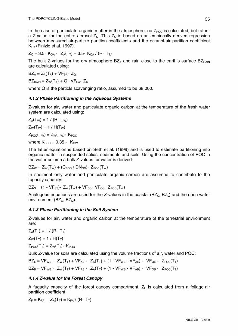
In the case of particulate organic matter in the atmosphere, no ZPOC is calculated, but rather a Z-value for the entire aerosol ZQ. This ZQ is based on an empirically derived regression between measured air-particle partition coefficients and the octanol-air partition coefficient KOA (Finizio et al. 1997).
ZQ = 3.5· KOA · ZA(TT) = 3.5· KOA / (R· TT)
The bulk Z-values for the dry atmosphere BZA and rain close to the earth’s surface BZRAIN are calculated using:
BZA = ZA(TA) + VFSA· ZQ
BZRAIN = ZW(TA) + Q· VFSA· ZQ
where Q is the particle scavenging ratio, assumed to be 68,000.
4.1.2 Phase Partitioning in the Aqueous Systems
Z-values for air, water and particulate organic carbon at the temperature of the fresh water system are calculated using:
ZA(TW) = 1 / (R· TW)
ZW(TW) = 1 / H(TW)
ZPOC(TW) = ZW(TW)· KPOC
where KPOC = 0.35 · KOW
The latter equation is based on Seth et al. (1999) and is used to estimate partitioning into organic matter in suspended solids, sediments and soils. Using the concentration of POC in the water column a bulk Z-values for water is derived:
BZW = ZW(TW) + (CPOC / DNOC)· ZPOC(TW)
In sediment only water and particulate organic carbon are assumed to contribute to the fugacity capacity:
BZS = (1 - VFSS)· ZW(TW) + VFSS· VFOS· ZPOC(TW)
Analogous equations are used for the Z-values in the coastal (BZC, BZL) and the open water environment (BZO, BZM).
4.1.3 Phase Partitioning in the Soil System
Z-values for air, water and organic carbon at the temperature of the terrestrial environment are:
ZA(TT) = 1 / (R· TT)
ZW(TT) = 1 / H(TT)
ZPOC(TT) = ZW(TT)· KPOC
Bulk Z-value for soils are calculated using the volume fractions of air, water and POC:
BZE = VFWE · ZW(TT) + VFAE · ZA(TT) + (1 - VFWE - VFAE) · VFOE · ZPOC(TT)
BZB = VFWB · ZW(TT) + VFAB · ZA(TT) + (1 - VFWB - VFAB) · VFOB · ZPOC(TT)
4.1.4 Z-value for the Forest Canopy
A fugacity capacity of the forest canopy compartment, ZF is calculated from a foliage-air partition coefficient.
ZF = KFA · ZA(TT) = KFA / (R· TT)

The POPCYCLING-Baltic Model
NILU OR 10/2000
36
Horstmann and McLachlan (1998) empirically determined partition coefficients KFA of several POPs for two forest canopies and regressed it against the octanol-air partition coefficient KOA.
KFA = M · KOAN
The regression parameters M and N were 14 and 0.76 for a deciduous canopy, and 38 and 0.69 for a coniferous canopy, giving a Z-value for a deciduous and a coniferous canopy, ZFdec and ZFcon. The bulk Z-value of the forest canopy BZF consisting of coniferous and deciduous trees is calculated using a volume fraction of coniferous leaves in the forest canopy VFconF, which is a time variant parameters (see above):
BZF = (1 - VFconF) · ZFdec + VFconF · ZFcon
4.2 Description of Chemical Processes in the POPCYCLING-Baltic Model
Transport and degradation processes in fugacity-based models are described with the help of D-values in units of mol/(Pa· h) (Mackay, 1991). There are principally three types of processes:
• advective transport processes
• diffusive transport processes, and
• degradation processes.
4.2.1 Description of Advection Processes
D-values for the transport of contaminant with advected air, water and POC are simply expressed as the product of the transfer rate of the carrier medium in units of m3/h and its Z-value in units of mol/(m3· Pa) (Mackay, 1991).
DESCRIPTION OF ATMOSPHERIC ADVECTION
The bulk air Z-value is multiplied with the atmospheric advection rates to give atmospheric advection D-values for the exchange between the atmospheric compartments DAA, and the exchange between the atmospheric compartments and the atmosphere outside of the model boundaries DAut and DAin.
DXY = BZA · aGXY
DESCRIPTION OF ADVECTION IN WATER
The same approach is used for the run-off from fresh water to coastal water DWC, and the exchange between the marine compartments DCO, DOC, DCC, and DOO:
DXY = BZX · wGXY
DESCRIPTION OF SOIL-FRESH WATER EXCHANGE
The run-off from soil to fresh water is calculated as the sum of contaminant advected with run-off water and contaminant advected with eroded particulate organic matter.
DEW = wGEW · ZW(TT) + oGEW · ZPOC(TT)
DBW = wGBW · ZW(TT) + oGBW · ZPOC(TT)
DESCRIPTION OF SEDIMENT BURIAL
Fresh water sediment burial is treated like a advected transport process using the POC burial rate calculated within the POC budget calculation and the Z-value for POC:
DLS = oGWbur· ZPOC

The POPCYCLING-Baltic Model
NILU OR 10/2000
37
Analogous equations are used for burial in coastal and deep marine sediments, DLL and DLM.
DESCRIPTION OF LITTER FALL
The transport of contaminant from the foliage to the soil with litter fall is another advective transport process. It is described as the product of the litter fall rate in m3 leaves/h and the foliage Z-value. The overall DFB is a weighted fraction of the coniferous and deciduous component:
DFB = fraFcon · GFBcon · ZFcon + (1 - fraFcon) · GFBdec · ZFdec
4.2.2 Description of Air-Surface Exchange
Three primary mechanisms of air-surface exchange of POPs are considered in the model: dry particle deposition, wet deposition, and diffusive gas exchange (deposition and evaporation). Parameters used to describe the exchange of POPs to various surfaces vary widely, and the selection of proper values is difficult. In order to assure consistency among the various parameters related to atmospheric deposition, we decided to use - whenever possible - kinetic parameters derived in the field by one research group, namely the Ecological Chemistry and Geochemistry research group at the University of Bayreuth. This group has made measurements of deposition velocities to forest canopies, bare soils and grasslands at a location in Southern Germany (Schröder et al., 1997, Horstmann and Mclachlan, 1998). Although this location is not within the Baltic Sea drainage basin, its climatic characteristics and vegetation cover is comparable to that found in the southern half of the Baltic Sea environment.
DESCRIPTION OF DRY PARTICLE DEPOSITION
Dry deposition of chemical associated with atmospheric particles to all surface compartments X is calculated using dry particle deposition velocities vXD-P in m/h:
DAX-P = AX · vXD-P · VFSA · ZQ
where AX is the surface area of the compartment and VFSA is the volume fraction of solids in the atmosphere.
A dry particle deposition velocity is the sum of a sedimentary component caused by the deposition of relatively large particles and a component deriving from the impaction and diffusion of relatively small particles. Whereas the latter is dependent on surface characteristics, the former is more or less independent of the type of the surface and is assumed to be 0.71 m/h throughout the entire model area (except to forest soils). This value was experimentally derived for the deposition of a whole range of POPs to a bare soil surface (Schröder et al., 1997).
The maximum dry particle deposition velocity to agricultural soil due to the impaction and diffusion of relatively small particles is assumed to be 0.32 m/h, which is also based on the measurements by Schröder et al. (1997). The dry particle deposition velocity to forest soils is assumed to be five times lower to account for the interception of particles by the canopy and the reduced atmospheric turbulence in the forest. The value of 0.32 m/h was also adopted for all water surfaces.
Deposition velocities of particle-bound POPs to forest canopies have so far been reported only by Horstmann and McLachlan (1998). They reported summer averaged deposition velocities due to the impaction and diffusion of small particles of 2.7 m/h for a spruce canopy and 26.3 m/h for a beech canopy. Although the latter value is high, it is not unreasonable considering that Gravenhorst and Waraghai (1990, as quoted in Umlauf and McLachlan, 1994) reported deposition velocites to a forest canopy (for particles with diameters between 0.8 and 20 µm) of 14.4 to 82.8 m/h.

The POPCYCLING-Baltic Model
NILU OR 10/2000
38
Table 11 summarises the dry particle deposition velocities to various surfaces that are used as default values in the model.
Table 11 Dry particle deposition velocities used as default values in the model.
Surface Due to sedimentation
due to impaction and diffusion
Total seasonally variable
Agricultural soil vED-P 0.71 0.32 1.03 Yes
Forest soil vBD-P 0.71 / 5 0.33 / 5 0.206 Yes
Coniferous canopy vFD-P 0.71 2.7 3.4 Yes
Deciduous canopy vFD-P 0.71 26.3 27.0 Yes
Water surface vWD-P 0.71 0.32 1.03 No
These deposition velocities can undergo a significant seasonal change. Often mass transfer to the terrestrial surface is reduced in winter driven by surface cooling and the absence of solar energy. This creates a more "stable" atmosphere which suppresses turbulence. Horstmann and McLachlan (1998) assumed for example that in Germany the more stable atmospheric conditions during winter reduce gaseous deposition velocities to forests by a factor of three. In the model, this is taken into account by defining a stability factor, facStability, which expresses the extent to which the winter atmosphere is more stable than the summer atmosphere. During summer vD equals vDmax, in winter vD is vDmax / facStability, and during spring and fall vD is interpolated between winter and summer values (Figure 17). The default value for facStability is assumed to be 3.
Deposition velocities to a deciduous canopy obviously undergo additionally large changes in time as a result of the seasonality of leaf development (Figure 16). vD to a deciduous canopy thus is additionally reduced by a factor reflecting the fraction of the canopy which stays on the trees during winter.
winterspring
summerfall
winter
deciduous canopyseasonality caused by changes in atmospheric stabilityand by seasonality of canopy development
coniferous canopy and soilsseasonality caused by changes in atmospheric stability
deposition velocities
Figure 17 Schematic representation of the seasonal dependence of the deposition velocities in the terrestrial environment. Values of vD are at a maximum during summer. During winter the summer average is reduced by a factor describing the relative stability of the atmosphere. During spring and fall, deposition velocities are derived by linear interpolation of summer and winter values.

The POPCYCLING-Baltic Model
NILU OR 10/2000
39
DESCRIPTION OF WET DEPOSITION
Wet deposition is treated as an advective transport process, and the D-value is simply the product of the rain water flow to a surface wGAX (in m3/h) and the bulk Z-value of rain BZrain (in mol/(Pa· m3)). No distinction is made between various forms of precipitation, such as snow or hail.
As is the case for other surfaces, wet deposition to the canopy occurs by vapour absorption in the rainwater and scavenging of particle-sorbed chemical. We further make two assumptions concerning wet deposition of POPs to the forest canopy:
1. the intercepted water dripping or flowing from the canopy to the soil has the same chemical concentration (in the dissolved phase and sorbed onto particles) as the original precipitation.
2. the amount of chemical in the water evaporating from the canopy is negligible.
This implies that the amount of chemical which was originally present in the water evaporating from the canopy is taken up in the leaves. Then the D-value expression describing the wet deposition of contaminant to the foliage is:
DAF-W = frUF · wGAF · BZrain
where frUF represents the fraction of the precipitation to the canopy that evaporates from the canopy.
DESCRIPTION OF DIFFUSIVE AIR-WATER EXCHANGE
Diffusive air-water exchange in all three types of water compartments is calculated based on the standard two-film theory (Liss and Slater, 1974, Mackay and Leinonen, 1975) invoking two mass transfer coefficients in series, U1 (in m/h) for the stagnant atmospheric boundary layer and U2 (in m/h) for the stagnant water layer close to the air-water interface. These mass transfer coefficients are calculated as a function of wind speed using relationships by Mackay and Yuen (1983) as quoted in Schwarzenbach et al. (1993).
U1 = 0.065 · (6.1+0.63· WS)0.5 · WS· 36
U2 = 0.000175 · (6.1 + 0.63 · WS)0.5 · WS· 36
The D-values for volatilisation from water are then calculated using
D = A
1U Z (T )
+ 1
U Z (T )
WAW
1 A W 2 W W⋅ ⋅
As detailed above, transfer from the atmosphere to the water surface can additionally occur by wet deposition and dry particle deposition, thus the D-value for total deposition to a water surface is:
DAW = DWA + AW · vWD-P · VFSA · ZQ + wGAW · BZrain
Equivalent equations are used for DCA, DAC, DOA, and DAO.
In the fresh and marine environment, different approaches are used to account for the influence of an ice cover. In the fresh water environment, diffusive gas exchange with the atmosphere ceases when the terrestrial air temperature drops below -2 °C, based on the assumption that an impenetrable ice cover forms at the temperature. In the marine environment, the D-values for diffusive gas exchange are reduced by the fraction of the water surface, that is ice-covered. This ice covered fraction is calculated as a function of the marine air temperatures TO and TC. Neither wet deposition, nor dry particle deposition is assumed to be affected by an ice cover.

The POPCYCLING-Baltic Model
NILU OR 10/2000
40
DESCRIPTION OF AIR-FOREST CANOPY-FOREST SOIL EXCHANGE
In studies with coniferous trees (Umlauf et al 1994) and grass (Welsch-Pausch et al. 1995), gaseous dry deposition was identified as the most important pathway of foliar uptake of semivolatile organic compounds. In deriving a D-value describing foliar uptake of gaseous chemical from the atmosphere we adopt the approach by McLachlan and Horstmann (1998) and convert to fugacity terms:
DAF-G = vFD-G · AB · ZA
where vFD-G is a dry gaseous deposition velocity or mass transfer coefficient describing transport from air to forest canopy in m/h and AB is the surface area of the soil in m2. The deposition velocity vFD-G includes stomatal uptake of vapour as well as gas absorption in the cuticle, the latter process being far more significant for hydrophobic chemicals. Measured deposition velocity vFD-G to forest canopies are considerably higher than for open surfaces (Table 12), which is the justification to treat a forested surface different from how deposition to terrestrial surfaces has been described traditionally in fugacity models.
Table 12 Measured dry gaseous deposition velocities for semi-volatile POPs reported in the literature.
Surface vD-G m/h Reference
Spruce canopy (annual average) 28.1 Horstmann and McLachlan, 1998
Beach/oak canopy (summer average) 129.6 Horstmann and McLachlan, 1998
Flat soil surface 2 Schröder et al., 1997
Grassland 2 McLachlan, 1996
Rye grass in pots 18 McLachlan et al., 1995
Average for seven grassland species 5 Böhme et al. 1999
These deposition velocities undergo a significant seasonal change for the same reasons as the dry particle deposition velocities (Figure 17) and the atmospheric stability factor and the fraction of deciduous leaves staying on the tree during winter are employed in an identical manner. To obtain a summer average of the dry gaseous deposition velocities to a coniferous canopy, the annual average given by Horstmann and McLachlan (1998) was multiplied by 1.5, giving 42.1 m/h.
Adding the terms describing dry particle and wet deposition, the composite D-value for foliar uptake is:
DAF = vFD-G · AB · ZA + AB · vFD-P · VFSA · ZQ + frUF · wGAF · BZrain
The D-value for evaporation from the foliage is the same as the one defined above for gas absorption:
DFA = vFD-G · AB · ZA
DESCRIPTION OF DIFFUSIVE AIR-SOIL EXCHANGE
In the classical approach to describe diffusive air-soil exchange in multimedia mass balance models (Mackay and Stiver, 1991, Jury et al. 1983), the two-resistances in series model of air water exchange is modified using a resistance in the stagnant air boundary layer over the soil and two parallel resistance to diffusion within the soil. We adopt a nomenclature of U7 for the mass transfer coefficient through the atmospheric boundary layer, U5 for diffusion in the air pore space and U6 in the water-filled pore space. The D-value for evaporation of chemical from soil then is:

The POPCYCLING-Baltic Model
NILU OR 10/2000
41
D = A
1U Z (T )
+ 1
U Z (T ) + U Z (T )
BAB
7 A T 5 A T 6 W T⋅ ⋅ ⋅
with an analogous equation for DEA.
Mass Transfer Coefficients over Soil
Typical values for the mass transfer coefficient U7 for the air boundary layer over soil used in models without forest compartments are 5 m/h (Mackay et al. 1992) and 2.5 to 10 (Wania and Mackay, 1995). In the POPCYCLING-Baltic model a maximum value U7Emax of 2.08 m/h is assumed to apply over agricultural soils, based on a value measured by Schröder et al., (1998). Over the forest soil, this mass transfer coefficient is assumed to be lower by a factor of 5 to a U7Bmax of 0.416 m/h due to the canopy effect. The atmospheric stability differences between summer and winter discussed above are taken into account by using the stability factor, facStability. During summer U7 equals U7max, in winter U7 is U7max / facStability, and during spring and fall U7 is interpolated between winter and summer values.
Mass Transfer Coefficients in Soil
Diffusion in soil water/soil air is modelled using a modification of the classical approach by Jury et al. (1983, 1984). The mass transfer coefficients for diffusion in the soil pore space U5 and in the water-filled pore space U6 are calculated using the molecular diffusion coefficients in air BA and water BW. These coefficients are relatively constant for POPs, and the values chosen by Jury et al. (1984) are used (0.018 and 0.0000018 m2· h-1, respectively). The diffusion path length in soil is taken as the log mean depth of the soil compartment, corrected for tortuosity using the Millington-Quirk formula:
Equivalent equations apply for U5E and U6E.
As pointed out recently (McLachlan and Wania, 1999), this classical approach is not applicable to the soil/air exchange of POPs, since it does not address processes such as bioturbation or ploughing that control the transport of chemicals with low mobility in the soil column. As an interim solution it was proposed that a minimum value for the mass transfer coefficient kS for transport within the soil be specified, based on estimates of the transport of solids in bulk soils (McLachlan and Wania, 1999).
In the POPCYCLING-Baltic model kS equals (U5· ZA(TT) + U6· ZW(TT)) / (VFOB · ZPOC(TT)).
If therefore U5· ZA(TT) + U6· ZW(TT) is smaller than VFOB · ZPOC(TT) · kSmin, where kSmin is the specified threshold for the diffusion in soil MTC, the D-value for soil to air diffusion is calculated using:
kSmin for agricultural soil is assumed to be 1 cm per year, in forest soils 0.5 cm per year.
Adding components for the advective deposition processes, the D-values describing total deposition to the soil compartments are:
DAE = DEA + AE · vED-P · VFSA · ZQ + wGAE · BZRAIN
DAB = DBA + AB · vBD-P · VFSA · ZQ + wGFB · BZRAIN

The POPCYCLING-Baltic Model
NILU OR 10/2000
42
4.2.3 Description of Water-Sediment Exchange
Three processes are assumed to contribute to the exchange of contaminants across the water-sediment interface in fresh water, coastal water and open water systems, namely:
• molecular diffusion in the aqueous phase
• bioturbation
• physical sedimentation and resuspension of particulate organic matter
All three processes act in either direction. Diffusion in the aqueous phase is described with the help of a diffusive mass transfer coefficient U8, which can be interpreted as the ratio of the diffusivity in water BW and a diffusion path length (calculated as log mean depth of the sediment compartment depth hS).
U = B(1 - VF )
0.390865 h8 WSS
1.5
S⋅
⋅
Bioturbation is treated as a pseudo-diffusive process invoking an equivalent “bioturbation diffusivity” Bbio.
U = B
0.390865 h8biobio
S⋅
Finally, sedimentation and resuspension is described as an advective transport process using the particulate organic carbon transport rates in m3/h derived in the POC balance calculation. The total water sediment D-values thus are:
DWS = AS· U8· ZW + AS· U8bio· ZPOC + oGsed· ZPOC
DSW = AS· U8· ZW + AS· U8bio· ZPOC + oGres· ZPOC
4.2.4 Description of Degradation Processes
D-values for degradation processes in fugacity terms are calculated as the product of a Z-value, the compartment volume and a first-order degradation rate k in units of h-1. In the POPCYCLING model all degradation rates are calculated as function of the compartment temperature.
DESCRIPTION OF ATMOSPHERIC DEGRADATION
The reaction of the chemical in the gas phase with hydroxyl radicals is assumed to be the only significant degradation pathway for POPs in the atmosphere (Atkinson, 1996). The degradation rate kRA is calculated as a function of seasonally variable atmospheric OH radical concentrations [OH] and temperatures TA, requiring a contaminant-specific degradation rate kRAref at the reference temperature 25°C and an activation energy AEA.
kRA = kRAref · [OH] · 3600 s/h · Exp(AEA / R · (1 / 298.15 - 1 / TA))
The D-value is calculated using this reaction rate constant and the gas phase Z-value only:
DRA = kRA · VA · ZA
DEGRADATION IN OTHER MEDIA
Degradation rates in other compartments are calculated as a function of temperature using a contaminant-specific degradation rate kRXref at the reference temperature 25°C and an activation energy AEX. This degradation rate is assumed to include all degradation processes that the POP can undergo, including biodegradation, hydrolysis, and photolysis.
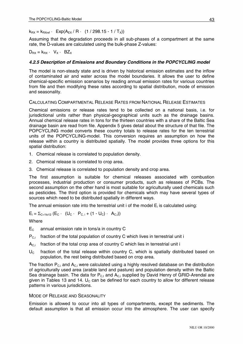
The POPCYCLING-Baltic Model
NILU OR 10/2000
43
kRX = kRXref · Exp(AEX / R · (1 / 298.15 - 1 / TX))
Assuming that the degradation proceeds in all sub-phases of a compartment at the same rate, the D-values are calculated using the bulk-phase Z-values:
DRX = kRX · VX · BZX
4.2.5 Description of Emissions and Boundary Conditions in the POPCYCLING model
The model is non-steady state and is driven by historical emission estimates and the inflow of contaminated air and water across the model boundaries. It allows the user to define chemical-specific emission scenarios by reading annual emission rates for various countries from file and then modifying these rates according to spatial distribution, mode of emission and seasonality.
CALCULATING COMPARTMENTAL RELEASE RATES FROM NATIONAL RELEASE ESTIMATES
Chemical emissions or release rates tend to be collected on a national basis, i.e. for jurisdictional units rather than physical-geographical units such as the drainage basins. Annual chemical release rates in tons for the thirteen countries with a share of the Baltic Sea drainage basin are read from file. Appendix 5 gives detail about the structure of that file. The POPCYCLING model converts these country totals to release rates for the ten terrestrial units of the POPCYCLING-model. This conversion requires an assumption on how the release within a country is distributed spatially. The model provides three options for this spatial distribution:
1. Chemical release is correlated to population density.
2. Chemical release is correlated to crop area.
3. Chemical release is correlated to population density and crop area.
The first assumption is suitable for chemical releases associated with combustion processes, industrial production or consumer products, such as releases of PCBs. The second assumption on the other hand is most suitable for agriculturally used chemicals such as pesticides. The third option is provided for chemicals which may have several types of sources which need to be distributed spatially in different ways.
The annual emission rate into the terrestrial unit i of the model Ei is calculated using:
Ei = ΣC=1to12 (EC · (UC · PC, i + (1 - UC) · AC,i))
Where
EC annual emission rate in tons/a in country C
PC,i fraction of the total population of country C which lives in terrestrial unit i
AC,i fraction of the total crop area of country C which lies in terrestrial unit i
UC fraction of the total release within country C, which is spatially distributed based on population, the rest being distributed based on crop area.
The fraction PC,i and AC,i were calculated using a highly resolved database on the distribution of agriculturally used area (arable land and pasture) and population density within the Baltic Sea drainage basin. The data for PC,I and AC,i supplied by David Henry of GRID-Arendal are given in Tables 13 and 14. UC can be defined for each country to allow for different release patterns in various jurisdictions.
MODE OF RELEASE AND SEASONALITY
Emission is allowed to occur into all types of compartments, except the sediments. The default assumption is that all emission occur into the atmosphere. The user can specify

The POPCYCLING-Baltic Model
NILU OR 10/2000
44
fractions, which distribute the annual emission rates into the ten terrestrial/coastal units (read from file) among the compartments air, forest canopy, forest soil, agricultural soil, fresh water and coastal water. Obviously, these fractions have to add up to one. These fractions are assumed fixed in time, but are allowed to vary from one region to another.
The default assumption is that the annual emissions are distributed evenly across the entire year. However, it is possible to modulate this by superimposing a sinusoidal function on the emission rates. The user can specify the amplitude (as a fraction of the mean) and the month of maximum emission. Again, these parameters are fixed from year to year, but can vary between the various regions.
Finally, the model allows the user to specify a region-specific, time-invariant scaling factor, which facilitates the modellling of contaminant mixtures. If the annual release rates is for a mixture of POPs (e.g. an Aroclor mixture), the scaling factor could be the fraction of that mixture, which is a certain constituent (e.g. a PCB congener or homologue).
In the model time variant emission rates EX into 59 compartments in units of mol/h are calculated, which are parameters in the mass balance equations (Table 15).
BOUNDARY CONDITIONS
POPs enter the Baltic Sea drainage basin with air and sea water advected into the region. The user may specify time invariant fugacity values in these incoming media, including the option to assume fugacities of 0 Pa, which implies no import of chemical from outside of the drainage basin. However, often the concentration in these media is not very well established, certainly not in a historical perspective.
This is why the model allows the user to specify ratios RfAut that relate the fugacities in the incoming flow with the calculated fugacities in the compartment receiving the inflow of air or water.
fAut = fA · RfAut
fO7 = fO6 · RfO
If these ratios are one, the system boundary acts like an inert wall returning just as much chemical into the drainage basin as has left by outbound advection (assuming similar temperature and phase composition i.e. VFSA and CpocO, inside and outside of the model region). A ratio greater than one implies a net import of contaminant, a ratio smaller than one a net outflow. Five such ratios (1 for each air compartment, 1 for the Skagerrak open water compartment) can be specified as a function of time in the file, that also supplies the annual emission rates (see above). These ratios may be estimated based on information of the relative magnitude of measured concentrations or estimated emissions on either side of the system boundary.

The POPCYCLING-Baltic Model
NILU OR 10/2000
45
Table 13 Fraction of the total agricuturally used area of a country that lies in one of the ten sub-basin as defined in the POPCYCLING model in percent.
Country T1 T2 T3 T4 T5 T6 T7 T8 T9 T10 Sum
Belarus 0 0 0 0.1 11.7 27.1 0 0 0 0 38.9
Czech. 0 0 0 0 0 11.1 0 0 0 0 11.1
Denmark 0 0 0 0 0 0 0 30.5 19.8 1.0 51.3
Estonia 0 0 66.1 0 22.3 11.6 0 0 0 0 100.0
Finland 27.4 32.7 21.2 16.8 0 0 0 0 0 0 98.1
Germany 0 0 0 0 0 1.8 0 1.7 0 0 3.5
Latvia 0 0 6.4 0 71.1 22.5 0 0 0 0 100.0
Lithuania 0 0 0 0 21.2 78.8 0 0 0 0 100.0
Norway 0.1 1.4 0 0 0 0 0 0 3.3 45.3 50.1
Poland 0 0 0 0 0 98.0 0 0 0 0 98.0
Russia 0 0 1.4 2.8 1.3 1.0 0 0 0 0 6.5
Sweden 1.6 12.9 0 0 0 0 43.8 5.8 34.1 1.8 100.0
Ukraine 0 0 0 0 0 3.5 0 0 0 0 3.5
Table 14 Fraction of the total population of a country that lives in one of the ten sub-basin as defined in the POPCYCLING model in percent.
Country T1 T2 T3 T4 T5 T6 T7 T8 T9 T10 Sum
Belarus 0 0 0 0.1 11.7 27.1 0 0 0 0 38.9
Czech. 0 0 0 0 0 11.1 0 0 0 0 11.1
Denmark 0 0 0 0 0 0 0 30.5 19.8 1.0 51.3
Estonia 0 0 82.1 0 13.3 4.6 0 0 0 0 100.0
Finland 18.3 28.1 38.0 13.2 0 0 0 0 0 0 97.6
Germany 0 0 0 0 0 1.5 0 2.0 0 0 3.5
Latvia 0 0 2.0 0 84.3 13.7 0 0 0 0 100.0
Lithuania 0 0 0 0 11.8 88.2 0 0 0 0 100.0
Norway 0.2 0.1 0 0 0 0 0 0 0.6 49.6 50.5
Poland 0 0 0 0 0 98.2 0 0 0 0 98.2
Russia 0.01 0 1.6 4.2 0.4 0.6 0 0 0 0 6.8
Sweden 4.7 14.0 0 0 0 0 44.2 8.0 27.9 1.2 100.0
Ukraine 0 0 0 0 0 3.5 0 0 0 0 3.5

The POPCYCLING-Baltic Model
NILU OR 10/2000
46
4.3 The Mass Balance Equations
4.3.1 The Mass Balance Equations
A linear non-steady state mass balance equation equals the change in inventory of a compartment with the sum of all input minus the sum of all outputs:
dM tdt
d V t Z t f tdt
( ) ( ( ) ( ) ( ))= ⋅ ⋅ ⋅= N (t) - D (t) f(t)I T
M(t) amount of chemical in a compartment at time t in mol
V(t) volume of a compartment at time t in m3
Z(t) Z-value of a compartment at time t in mol/(m3· Pa)
f(t) fugacity in a compartment at time t in Pa
Ni(t) total input rate into a compartment at time t in mol/h
DT(t) D-value for total loss from a compartment at time t in mol/(h· Pa)
Table 14 lists the equations for calculating the total input rates and the total loss D-values for all types of compartments. For reference appendix 4 lists the complete mass balance equation for all 85 model compartments individually.
4.3.2 The Solution of the Mass Balance Equations
Making a finite difference approximation, we get:
d V t t Z t t f t t V t Z t f tdt
(( ( ) ( ) ( )) ( ( ) ( ) ( )))+ ⋅ + ⋅ + − ⋅ ⋅ ⋅∆ ∆ ∆= N (t) - D (t) f(t)I T
The left hand side defines the change in inventory of the compartment. There is only one unknown in the above equation (f(t+∆t)) and hence it can be solved stepwise. The stepwise solution in the case of a compartment with fixed volume is:
f(t + t) = Z(t) f(t) + ((N (t) - D (t) f(t))
tV(t)
Z(t + t)
I T
∆
∆
∆
⋅ ⋅ ⋅
In the case of a compartment with time variable volume (i.e. the forest canopy):
f(t + t) = V(t) Z(t) f(t) + ((N (t) - D (t) f(t)) t
V(t + t) Z(t + t) I T∆
∆∆ ∆
⋅ ⋅ ⋅⋅
In the model the step size is variable within in the range of 1 to 24 hours. A minimum of 12 hours is recommended to reduce errors.

The POPCYCLING-Baltic Model
NILU OR 10/2000
47
Table 15 Equations for the total input rates NIX and total loss D-values DTX.
Compartment total input rates NIX total loss D-values DTX
Atmosphere NIA = EA + NvolA + Σ(DAA· fA) + DAin· fAut DTA = DRA + DdepA + Σ DAA + DAout
forest canopy NIF = EF + DAF· fA DTF = DRF + DFA + DFB
forest soil NIB = EB + DFB· fF + DAB· fA DTB = DRB + DBA + DBW
Agricultural soil NIE = EE + DAE· fA DTE = DRE + DEA + DEW
fresh water NIW = EW + DAW· fA + DBW· fB + DEW· fE + DSW· fS DTW = DRW + DWA + DWC + DWS
coastal water NIC = EC + DAC· fA + DWC· fW + DLC· fL + DOC· fO (+ DCC· fC)(A) DTC = DRC + DCA + DCL + DCO (+ DCC)(A)
open water NIO = EO + DAO· fA + DMO· fM + Σ(DCO· fC) + Σ (DOO· fO) DTO = DRO + DOA + DOM + Σ DOC + Σ DOO
fresh water sediment NIS = DWS· fW DTS = DRS + DLS + DSW
coastal sediment NIL = DCL· fC DTL = DRL + DLL + DLC
deep sediment NIM = DOM· fO DTM = DRM + DLM + DMO (A) intercoastal transfer occurs only between Kattegat and Danish Straits

The POPCYCLING-Baltic Model
NILU OR 10/2000
48
5. References
Andersson, A. and Rudehaell, Å. (1993) Proportion of plankton biomass in particulate organic carbon in the northern Baltic Sea. Mar. Ecol. Prog. Ser., 95, pp. 133-139.
Atkinson, R. (1996) Atmospheric chemistry of PCBs, PCDDs and PCDFs. In: Chlorinated Organic Micropollutants, ed. by R.E. Hester and R.M. Harrison. Cambridge, Royal Society of Chemistry. (Issues in environmental science and technology 6). pp. 53-72.
Axelman, J. (1997) Biological, physico-chemical and biogeochemical dynamics of hydro-phobic organic compounds. Doctoral thesis. Stockholm University.
Bakker, J.F. and Helder, W. (1993) Skagerrak (northeastern North Sea) oxygen microprofiles and porewater chemistry in sediments. Mar. Geol. 111, pp. 299 - 321.
Bengtsson, B.E., Nellbring, S., Hill, C., Kessler, E. (Eds.) (1999) Special Issue: Reproductive disturbances in Baltic Sea fish. An international perspective. Ambio, 28, pp. 1-107.
Bergström, S. and Carlsson, B. (1994) River runoff to the Baltic Sea: 1950-1990. Ambio, 23, pp. 280-287.
Bierman, V.J. and Swain, W.R. (1982) Mass balance modelling of DDT dynamics in Lakes Michigan and Superior. Environ. Sci. Technol., 16, pp. 572-579.
Bierman, V.J., Jr., DePinto, J.V., Young, T.C., Rodgers, P.W., Martin, S.C., Raghunathan, R.K. (1992) Development and validation of an intergrated exposure model for toxic chemicals in Green Bay, Lake Michigan. Report prepared for U.S. EPA. Grosse Ile, Michigan.
Broman, D., Näf, C., Rolff, C., Zebühr, Y. (1991) Occurrence and dynamics of polychlorinated dibenzo-p-dioxins and dibenzofurans in the mixed surface layer of remote coastal and offshore waters in the Baltic. Environ. Sci. Technol., 25, pp. 1850-1864.
Carman, R., Aigras, J., Larsen, B. (1996) Carbon and nutrient geochemistry of the surface sediments of the Gulf of Riga, Baltic Sea. Mar. Geol., 134, pp. 57-76.
Cowan, C., Mackay, D., Feijtel, T., van de Meent, D., Di Guardo, A., Davies, J., Mackay, N. (1995) The multi-media model: A vital tool for predicting the fate of chemicals. SETAC Pensacola Press.
Danielsson, Å, Carman, R., Rahm, L., Aigars, J. (1998) Spatial estimation of nutrient distributions in the Gulf of Riga sediments using Cokriging. Estuar. Coast. Shelf Sci., 48, pp. 713-722.
De Haas, H. and van Weering, T.C.E. (1997) Recent sediment accumulation, organic carbon burial and transport in the northeastern North Sea. Mar. Geol., 136, pp. 173-187.
Diamond, M., Poulton, D., Mackay, D., Stride, F. (1994) Development of a mass balance model of the fate of 17 chemicals in the Bay of Quinte. J. Great Lakes Res., 20, pp. 643-666.
Elmgren, R. (1984) Trophic dynamics in the enclosed, brackish Baltic Sea. Rapp. P.-v. Reun. Cons. Int. Explor. Mer., 183, pp. 151-169.
Finizio, A., Mackay, D., Bidleman, T.F., Harner, T. (1997) Octanol-air partition coefficient as a predictor of partitioning of semivolatile organic chemicals to aerosols. Atmos. Environ., 31, pp. 2289-2296.
Fonselius, S.H. (1991) Västerhavets och Östersjöns oceanografi. Stockholm Swedish Meteorological and Hydrological Institute.

The POPCYCLING-Baltic Model
NILU OR 10/2000
49
Forsgren, G. and Jansson, M. (1992) The turnover of river-transported iron, phosphorous and organic carbon in the Öre estuary, Northern Sweden. Hydrobiologia, 235/236, pp. 585-596.
Fraters, D., Bouwman, A.F., Thewessen, T.J.M. (1993) Soil organic matter map for Europe. Estimates of soil organic matter content of the topsoil of FAO-Unesco soil units. Bilthoven (RIVM Report 481505004).
Gobas, F.A.P.C., Z’Graggen, M.N., Zhang, X. (1995) Time response of the Lake Ontario ecosystem to virtual elimination of PCBs. Environ. Sci. Technol., 29, pp. 2038-2046.
HELCOM (1986) Water Balance of the Baltic Sea. (Baltic Sea Environment Proceedings 16).
Horstmann, M. and McLachlan, M.S. (1996) Evidence of a novel mechanism of semivolatile organic compound deposition in coniferous forests. Environ. Sci. Technol., 30, pp. 1794-1796.
Horstmann, M. and McLachlan, M.S. (1998) Atmospheric deposition of semivolatile organic compounds to two forest canopies. Atmos. Environ., 32, pp. 1799-1809.
Jensen, S., Johnels, A.G., Olsson, M., Otterlind, G. (1969) DDT and PCB in marine animals from Swedish waters. Nature, 224, p. 247.
Jury, W.A., Spencer, W.F., Farmer, W.J. (1983) Behaviour assessment model for trace organics in soil. I. Model description. J. Environ. Qual., 12, pp. 558-564.
Langaas, S. and Sweitzer, J. (1996) A baltic drainage basin GIS database for environmental description and analysis. Technical report from GRID-Arendal/Beijer Institute/ Department of Systems Ecology, with accompanying database on CD-ROM. Stockholm.
Liss, P.S. and Slater, P.G., (1974) Flux of gases across the air-sea interface. Nature, 247, pp. 181-184.
Lun, R., Lee, K., De Marco, L., Nalewajko, C., Mackay, D. (1998) A model of the fate of poly-cyclic aromatic hydrocarbons in the Saguenay Fjord, Canada. Environ. Toxicol. Chem., 17, pp. 333-341.
Mackay D. and Leinonen, P. (1975) The rate of evaporation of low solubility contaminants from water bodies. Environ. Sci. Technol., 9, pp. 1178-1180.
Mackay, D. and Yuen, A.T.K. (1983) Mass transfer coefficient correlations for volatilization of organic solutes from water. Environ. Sci. Technol., 17, pp. 211-216.
Mackay, D., Joy, M., Paterson, S. (1983) A quantitative water, air, sediment interaction (QWASI) fugacity model for describing the fate of chemicals in lakes. Chemosphere, 12, pp. 981-997.
Mackay, D. (1989) Modeling the long-term behaviour of an organic contaminant in a large lake: Application to PCBs in Lake Ontario. J. Great Lakes Res., 15, pp. 283-297.
Mackay, D. (1991) Multimedia environmental models. The fugacity approach. Chelsea, MI, Lewis.
Mackay, D. and Stiver, W. (1991) Predictability and environmental chemistry. In: Environmental Chemistry of Herbicides, Volume II. Ed. by R. Grover and A.J. Cessna. Boca Raton, FL, CRC Press. pp. 281-297.
Mackay, D., Paterson, S., Shiu, W.Y. (1992) Generic models for evaluating the regional fate of chemicals. Chemosphere, 24, pp. 695-717.
Mackay, D., Sang, S., Vlahos, P., Diamond, M.L., Gobas, F.A.P.C., Dolan, D. (1994) A rate constant model of chemical dynamics in a lake ecosystem. J. Great Lakes Res., 20, pp. 625-642.

The POPCYCLING-Baltic Model
NILU OR 10/2000
50
McLachlan, M.S. and Horstmann, M. (1998) Forest as filters of airborne pollutants: A model. Environ. Sci. Technol., 32, pp. 413-420.
McLachlan, M.S. and Wania, F. (1999) Modelling soil/air exchange of persistent organic pollutants. Environ. Sci. Technol.,submitted.
O’Connor, D.J. (1988) Models of sorptive substances in freshwater systems. II: Lakes and Reservoirs. J. Environ. Eng., 114, pp. 533-551.
Olesen, M. (1995) Comparision of the sedimentation of a diatom spring bloom and of a subsurface chlorophyll maximum. Mar. Biol., 121, pp. 541 -547.
Olsson, M., Karlsson, B., Ahnland, E. (Eds.) (1992) Special Issue: Seals and Seal Protection. Ambio, 21, No. 8.
Persson, J. (2000) POPCYCLING MODEL. Particulate organic carbon - data and literature. Spreadsheet “POCbudget.xls” prepared for POPCYCLING-Baltic project meeting, Oslo, Norway, March 18 - 19, 1999 (updated January 25, 2000).
Pitkaenen, H., Tamminen, T., Kangas, P., Huttula, T., Kivi, K., Kuosa, H., Sarkkula, J., Eloheimo, K., Kauppila, P., Skakalsky, B. (1993) Late summer trophic conditions in the north-east Gulf of Finland and the River Neva estuary, Baltic Sea. Estuar. Coast. Shelf Res., 37, pp. 453-474.
Rodriguez, J.M., Ko, M.K.W., Sze, N.D., Heisey, C.W. (1992) Impact of biomass burning on tropospheric CO and OH. A two-dimensional study. In: Global biomass burning, atmospheric, climatic, and biological implications. Ed. by J.S. Levine. Cambridge, MIT Press, pp. 351-359.
Rydberg, L., Edler, L., Floderus, S., Graneli, W. (1990) Interaction between supply of nutrients, primary production, sedimentation and oxygen consumption in SE Kattegat. Ambio, 19, pp. 134-141.
Schröder, J., Welsch-Pausch, K., McLachlan, M.S. (1997) Measurement of atmospheric deposition of polychlorinated dibenzo-p-dioxins (PCDDs) and dibenzofurans (PCDFs) to a soil. Atmos. Environ., 31, pp. 2983-2989.
Schwarzenbach, R.E., Gschwend, P.M., Imboden, D.M. (1993) Environmental Organic Chemistry. New York, Wiley.
Seth, R., Mackay, D., Muncke, J. (1999) Estimating the organic carbon partition coefficient and its variability for hydrophobic chemicals. Environ. Sci. Technol., 33, pp. 2390-2394.
SLU (1999). Department of Environmental Assessment, Swedish Agricultural University. http://www.ma.slu.se/index.phtml.en, updated 99-11-18.
Sonzogni, W.C., Canole, R.P., Lam, D.C.L., Lick, W., Mackay, D., Minns, C.K., Richardson, W.L., Scavia, D., Smith, V., Strachan, W.M.J. (1987). Large lake models - uses, abuses and future. J. Great Lakes Res., 13, pp. 387-396.
Stigebrandt, A. (1991) Computations of oxygen fluxes through the sea surface and the net production of organic matter with application to the Baltic and adjacent seas. Limnol. Oceanogr., 36, pp. 444-454.
Stigebrandt, J. and Wulff, F. (1987) A model for the dynamics of nutrients and oxygen in the Baltic proper. J. Mar. Res., 45, pp. 729-759.
Sweitzer, J., Langaas, S., Folke, C. (1996) Land cover and population density in the Baltic Sea drainage basin: A GIS data base. Ambio, 25: pp. 191-198.
Thomann, R.V. and Di Toro, D.M. (1983) Physico-chemical model of toxic substances in the Great Lakes. J. Great Lakes Res., 9, pp. 474-496.

The POPCYCLING-Baltic Model
NILU OR 10/2000
51
Thomann, R.V. (1998) The future “golden age” of predictive models for surface water quality and ecosystem management. J. Environ. Eng., 124, pp. 94-103.
Tuomi, P., Suominen, K., Autio, R. (1999) Phytoplankton and bacterioplankton production and bacterial biomass in a fjord-like bay - open sea gradient. Hydrobiologia, 393, pp. 141-150.
Umlauf, G., Hauk, H., Reisinger, M. (1994) Deposition of semivolatile organic compounds to spruce needles. II. Experimental evaluation of the relative importance of different pathways. Environ. Sci. & Pollut. Res., 1, pp. 209-222.
Wallin, M. and Håkansson, L. (1992) Morphometry and sedimentation as regulating factors for nutrient recycling and trophic state in coastal waters. Hydrobiologia, 235/236, pp. 33-45.
Wania, F. and Mackay, D. (1995) A global distribution model for persistent organic chemicals. Sci. Total Environ., 160/161, pp. 211-232.
Wania, F. (1996) Spatial variability in compartmental fate modelling: Linking fugacity models and GIS. Environ. Sci. & Pollut. Res., 3, pp. 39-46.
Wania, F., Haugen, J.-E., Lei, Y.D., Mackay, D. (1998) Temperature dependence of atmos-pheric concentrations of semi-volatile organic compounds. Environ. Sci. Technol., 32, pp. 1013-1021.
Wania F., Broman, D., Axelman, J., Näf, C., Agrell, C. (1999) A multi compartmental, multi-basin fugacity model describing the fate of PCBs in the Baltic Sea. In: A Systems Analysis of the Changing Baltic Sea. Ed. by F. Wulff, P. Larsson and L. Rahm. Springer, in press.
Wania, F. and Mackay, D. (1999) The evolution of mass balance models of persistent organic pollutant fate in the environment. Environ. Pollut., 100, pp. 223-240.
Wassman, P. (1990a) Calculating the load of organic carbon to the aphotic zone in eutrophicated coastal waters. Mar. Pollut. Bull., 21, pp. 183-187.
Wassman, P. (1990b) Relationship between primary and export production in the boreal coastal zone of the North Atlantic. Limnol. Oceanogr., 35, pp. 464-471
Wassman, P. (1984) Sedimentation and benthic mineralization of organic detritus in a Norwegian fjord. Mar. Biol., 83, pp. 83-94.
Welsch-Paul, K., McLachlan, M.S., Umlauf, G. (1995) Determination of the principal pathways of polychlorinated dibenzo-p-dioxins and dibenzofurans to Lolium multiflorum (Welsh rye grass). Environ. Sci. Technol., 29, pp. 1090-1098.
Wulff, F., Rahm, L., Jonsson, P., Brydsten, L., Ahl, T., Granmo, Å. (1993) A mass-balance model of chlorinated organic matter for the Baltic Sea - A challenge for ecotoxicology. Ambio, 22, pp. 27-31.

The POPCYCLING-Baltic Model
NILU OR 10/2000
52
Appendix 1: Glossary
Environmental Properties
Compartment dimensions AX surface area of compartment X in m2 hX depth of compartment X in m VX volume of compartment X in m3
Volume fractions in m3/m3 VFSA volume fraction of aerosols in atmosphere VFconFvolume fraction of coniferous foliage in forest canopy compartment VFSS volume fraction of solids in sediment (equivalent for VFSL and VFSM) VFOS volume fraction of organic carbon in sediment solids VFWE volume fraction of water in agricultural soil VFAE volume fraction of air in agricultural soil VFOE volume fraction of organic carbon in agricutural soil solids VFWB volume fraction of water in forest soil VFAB volume fraction of air in forest soil VFOB volume fraction of organic carbon in forest soil solids CPOCX concentration of POC in water compartment X in units of g/m3
OCX mass fraction organic carbon in solids of compartment X
DNOC density of organic carbon in g/m3
DNMM density of mineral matter in g/m3 [OH] OH concentration is in units of molecules/cm3 TA atmospheric temperature in K TW temperature of fresh water in K TT temperature of terrestrial environment in K R ideal gas constant in units of J/(K· mol)
Transport Parameters Q particle scavenging ratio (dimensionless)
Mass transfer coefficients in m/h U1 mass tranfer coefficient for the stagnant atmospheric boundary layer over water in m/h U2 mass transfer coefficient for the stagnant water layer at the air-water interface in m/h vFD-G gaseous deposition velocity to the forest canopy in m/h vFD-P particle deposition velocity to the forest canopy in m/h vED-P particle deposition velocity to the agricultural soil in m/h vBD-P particle deposition velocity to the forest soil in m/h vWD-P particle deposition velocity to a water surface in m/h U8 mass transfer coefficient for diffusion across the air-sediment interface in m/h U8bio mass transfer coefficient for bioturbation in m/h

The POPCYCLING-Baltic Model
NILU OR 10/2000
53
Diffusivities in m2/h BW molecular diffusivity in air in m2/h BA molecular diffusivity in water in m2/h Bbio bioturbation diffusivity in units of m2/h
wGXY water advection rates from compartment X to compartment Y in units of m3/h wGAF precipitation to canopy wGFA evaporation from canopy wGFB throughfall/stem flow wGBA evaporation from forest soil wGBW run-off/leaching from forest soil wGAE precipitation to agricultural soil wGEA evaporation from agricultural soil wGEW run-off/leaching from agricultural soil wGAW precipitation to fresh water wGWA evaporation from fresh water wGWC riverine run-off
frUX fraction of precipitation to a compartment that evaporates from that compartment
oGX flux or rate of POC within aquatic system X in units of m3 POC/h (X = W for fresh water, C for coastal water and O for open water) oGXpro primary production of POC within system oGXin import of POC from outside the system oGXout export of POC out of the system oGXmiw POC mineralisation in the water column oGXsed POC settling to the sediments oGXres POC resuspension from sediments oGXmis POC mineralisation in surface sediment oGXbur POC sediment burial
oGEW run-off of POC from agricultural soil to fresh water oGBW run-off of POC from forest soil to fresh water oGWC run-off of POC from fresh water to coastal water
Other advective transfer rates in m3/h aGXY air advection rate from compartment X to compartment Y GFB litterfall term in m3 leaves/h
Chemical Properties H Henry’s law constant in Pa· mol/m3 KOW octaonl-water partition coefficient KOA octanol-air partition coefficient (dimensionless) KPOC partition coefficient between particulate organic carbon and water
(dimensionless) KFA foliage-air partition coefficient (dimensionless)
kRA reaction rate in air in units of h-1 kRAref reaction rate in air at 25°C in units of cm3/(molecules· s) AEA activation energy of the reaction with OH radicals in J/mol kRX reaction rate in phase X in units of h-1 kRXref reaction rate in phase X at 25°C in units of h-1 AEX activation energy of the degradation reaction in J/mol fX fugacity in compartment X in Pa

The POPCYCLING-Baltic Model
NILU OR 10/2000
54
Z-values in mol/(m3· Pa)
ZA Z-value for pure air ZW Z-value of water ZPOC Z-value of particulate organic carbon ZQ Z-value for the aerosol phase ZFdec Z-value for deciduous forest canopy ZFcon Z-value for coniferous forest canopy
BZX bulk Z-value of compartment X BZRAINbulk Z-value of rain water BZF bulk Z-value for forest canopy (foliage)
D-Values in units of mol/(h· Pa) DAF D-value for air to forest canopy transfer DAB D-value for air to forest soil transfer DAE D-value for air to agricultural soil transfer DAW D-value for air to fresh water transfer DAC D-value for air to coastal water transfer DAO D-value for air to open water transfer DFB D-value for forest canpy to forest soil transfer DBW D-value for forest soil to fresh water transfer DEW D-value for agricultural soil to fresh water transfer DWS D-value for fresh water to sediment transfer DSW D-value for sediment to fresh water transfer DCL D-value for coastal water to sediment transfer DLC D-value for sediment to coastal water transfer DOM D-value for open water to deep sediment transfer DMO D-value for deep sediment to open water transfer DWS D-value for fresh water to sediment transfer DLS D-value for fresh water sediment burial DLL D-value for coastal sediment burial DLM D-value for deep sediment burial DCO D-value for coastal water to open water transfer DCO D-value for open water to coastal water transfer DOO D-value for transfer between open water compartments DCC D-value for transfer between coastal water compartments DAA D-value for transfer between atmospheric compartments DAin D-value for atmospheric advection into the model region DAut D-value for atmospheric advection out of the model region DRX D-value for degradation loss from compartment X
DTX D-value for total loss from compartment X DdepA D-value for the sum of all deposition processes from an atmospheric compartment DvolA D-value for the sum of all volatilisation processes into an atmospheric compartment

The POPCYCLING-Baltic Model
NILU OR 10/2000
55
Appendix 2: Mass Balance Equations
In the following the complete 85 mass balance equations for the contaminant in the POPCYCLING-model are listed:
Atmospheric Compartments
Northern Atmosphere:
dMA1/dt = EA1 + DFA1· fF1 + DBA1· fB1+ DEA1· fE1 + DWA1· fW1 + DCA1· fC1 + DFA2· fF2 + DBA2· fB2+ DEA2· fE2 + DWA2· fW2 + DCA2· fC2 + DO1A1· fO1 + DO2A1· fO2 + DA4A1· fA4 + DA2A1· fA2 + DAin1· fAut1 - fA1 · (DRA1 + DAF1 + DAB1 + DAE1 + DAW1 + DAC1 + DAF2 + DAB2 + DAE2 + DAW2 + DAC2 + DA1O1 + DA1O2 + DA1A4 + DA1A2 + DAut1)
Eastern Atmosphere:
dMA2/dt = EA2 + DFA3· fF3 + DBA3· fB3+ DEA3· fE3 + DWA3· fW3 + DCA3· fC3 + DFA4· fF4 + DBA4· fB4+ DEA4· fE4 + DWA4· fW4 + DCA4· fC4 + DFA5· fF5 + DBA5· fB5+ DEA5· fE5 + DWA5· fW5 + DCA5· fC5 + DO3A2· fO3 + DA1A2· fA1 + DA3A2· fA3 + DAin2· fAut2 - fA2 · (DRA2 + DAF3 + DAB3 + DAE3 + DAW3 + DAC3 + DAF4 + DAB4 + DAE4 + DAW4 + DAC4 + DAF5 + DAB5 + DAE5 + DAW5 + DAC5 + DA2O3 + DA2A1 + DA2A3 + DAut2)
Southern Atmosphere:
dMA3/dt = EA3 + DFA6· fF6 + DBA6· fB6+ DEA6· fE6 + DWA6· fW6 + DCA6· fC6 + DO4A3· fO4 + DA2A3· fA2 + DA4A3· fA4 + DAin3· fAut3 - fA3 · (DRA3 + DAF6 + DAB6 + DAE6 + DAW6 + DAC6 + DA3O4 + DA3A2 + DA3A4 + DAut3)
Western Atmosphere:
dMA4/dt = EA4 + DFA7· fF7 + DBA7· fB7+ DEA7· fE7 + DWA7· fW7 + DCA7· fC7 + DFA8· fF8 + DBA8· fB8+ DEA8· fE8 + DWA8· fW8 + DCA8· fC8 + DFA9· fF9 + DBA9· fB9+ DEA9· fE9 + DWA9· fW9 + DCA9· fC9 + DFA10· fF10 + DBA10· fB10+ DEA10· fE10 + DWA10· fW10 + DCA10· fC10 + DO4A4· FO4 + DO6A4· fO6 + DA3A4· fA3 + DA1A4· fA1 + DAin4· fAut4 - fA4 · (DRA4 + DAF7 + DAB7 + DAE7 + DAW7 + DAC7 + DAF8 + DAB8 + DAE8 + DAW8 + DAC8 + DAF9 + DAB9 + DAE9 + DAW9 + DAC9 + DAF10 + DAB10 + DAE10 + DAW10 + DAC10 + DA4O4 + DA4O6 + DA4A3 + DA4A1 + DAut4)
Coastal Water Compartments
Coastal Bothnian Bay:
dMC1/dt = EC1 + DAC1· fA1 + DWC1· fW1 + DLC1· fL1 + DO1C1· fO1 - fC1 · (DRC1 + DCL1 + DCA1 + DC1O1)
Coastal Bothnian Sea:
dMC2/dt = EC2 + DAC2· fA1 + DWC2· fW2 + DLC2· fL2 + DO2C2· fO2 - fC2 · (DRC2 + DCL2 + DCA2 + DC2O2)
Coastal Gulf of Finland:
dMC3/dt = EC3 + DAC3· fA2 + DWC3· fW3 + DLC3· fL3 + DO3C3· fO3 - fC3 · (DRC3 + DCL3 + DCA3 + DC3O3)
Coastal Neva:
dMC4/dt = EC4 + DAC4· fA2 + DWC4· fW4 + DLC4· fL4 + DO3C4· fO3 - fC4 · (DRC4 + DCL4 + DCA4 + DC4O3)

The POPCYCLING-Baltic Model
NILU OR 10/2000
56
Coastal Gulf of Riga:
dMC5/dt = EC5 + DAC5· fA2 + DWC5· fW5 + DLC5· fL5 + DO4C5· fO4 - fC5 · (DRC5 + DCL5 + DCA5 + DC5O4)
Coastal Southern Baltic Proper:
dMC6/dt = EC6 + DAC6· fA3 + DWC6· fW6 + DLC6· fL6 + DO4C6· fO4 - fC6 · (DRC6 + DCL6 + DCA6 + DC6O4)
Coastal Swedish Baltic Proper:
dMC7/dt = EC7 + DAC7· fA4 + DWC7· fW7 + DLC7· fL7 + DO4C7· fO4 - fC7 · (DRC7 + DCL7 + DCA7 + DC7O4)
Danish Straits:
dMC8/dt = EC8 + DAC8· fA4 + DWC8· fW8 + DLC8· fL8 + DO4C8· fO4 + DC9C8· fC9 - fC8 · (DRC8 + DCL8 + DCA8 + DC8C9 + DC8O4 + DC8O5)
Kattegat:
dMC9/dt = EC9 + DAC9· fA4 + DWC9· fW9 + DLC9· fL9 + DO6C9· fO6 + DC8C9· fC8 - fC9 · (DRC9 + DCL9 + DCA9 + DC9C8 + DC9O6)
Coastal Skagerrak:
dMC10/dt = EC10 + DAC10· fA4 + DWC10· fW10 + DLC10· fL10 + DO6C0· fO6 - fC10 · (DRC10 + DCL10 + DCA10 + DC10O6)
Open Water Compartments
Open Bothnian Bay:
dMO1/dt = EO1 + DA1O1· fA1 + DC1O1· fC1 + DO2O1· fO2 + DMO1· fM1 - fO1 · (DRO1 + DOM1 + DO1A1 + DO1C1 + DO1O2)
Open Bothnian Sea:
dMO2/dt = EO2 + DA1O2· fA1 + DC2O2· fC2 + DO1O2· fO1 + DO4O2· fO4 + DMO2· fM2 - fO2 · (DRO2 + DOM2 + DO2A1 + DO2C2 + DO2O1 + DO2O4)
Open Gulf of Finland:
dMO3/dt = EO3 + DA2O3· fA2 + DC3O3· fC3 + DC4O3· fC4 + DO4O3· fO4 + DMO3· fM3 - fO3 · (DRO3 + DOM3 + DO3A2 + DO3C3 + DO3C4 + DO3O4)
Open Baltic Proper:
dMO4/dt = EO4 + DA3O4· fA3 + DA4O4· fA4 + DC5O4· fC5 + DC6O4· fC6 + DC7O4· fC7 + DC8C4· fC8 + DO2O4· fO2 + DO3O4· fO3 + DO5O4· fO5 - fO4 · (DRO4 + DO4A3 + DO4A4 + DO4C5 + DO4C6 + DO4C7 + DO4C8 + DO4O2 + DO4O3 + DO4O5)
Baltic Proper Bottom Water:
dMO5/dt = DO4O5· fO4 + DC8O5· fC8 + DMO5· fM5 - fO5 · (DRO5 + DOM5 + DO5O4)
Open Skagerrak:
dMO6/dt = EO6 + DA4O6· fA4 + DC10O6· fC10 + DC9O6· fC9 + DO7O6· fO7 + DMO6· fM6 - fO6 · (DRO6 + DOM6 + DO6A4 + DO6C10 + DO6C9 + DO6O7)

The POPCYCLING-Baltic Model
NILU OR 10/2000
57
Forest Canopy Compartments
dMF1/dt = EF1 + DAF1· fA1 - fF1 · (DRF1 + DFA1 + DFB1) dMF2/dt = EF2 + DAF2· fA1 - fF2 · (DRF2 + DFA2 + DFB2) dMF3/dt = EF3 + DAF3· fA2 - fF3 · (DRF3 + DFA3 + DFB3) dMF4/dt = EF4 + DAF4· fA2 - fF4 · (DRF4 + DFA4 + DFB4) dMF5/dt = EF5 + DAF5· fA2 - fF5 · (DRF5 + DFA5 + DFB5) dMF6/dt = EF6 + DAF6· fA3 - fF6 · (DRF6 + DFA6 + DFB6) dMF7/dt = EF7 + DAF7· fA4 - fF7 · (DRF7 + DFA7 + DFB7) dMF8/dt = EF8 + DAF8· fA4 - fF8 · (DRF8 + DFA8 + DFB8) dMF9/dt = EF9 + DAF9· fA4 - fF9 · (DRF9 + DFA9 + DFB9) dMF10/dt = EF10 + DAF10· fA4 - fF10 · (DRF10 + DFA10 + DFB10)
Forest Soil Compartments dMB1/dt = EB1 + DAB1· fA1 + DFB1· fF1 - fB1 · (DRB1 + DBA1 + DBW1) dMB2/dt = EB2 + DAB2· fA1 + DFB2· fF2 - fB2 · (DRB2 + DBA2 + DBW2) dMB3/dt = EB3 + DAB3· fA2 + DFB3· fF3 - fB3 · (DRB3 + DBA3 + DBW3) dMB4/dt = EB4 + DAB4· fA2 + DFB4· fF4 - fB4 · (DRB4 + DBA4 + DBW4) dMB5/dt = EB5 + DAB5· fA2 + DFB5· fF5 - fB5 · (DRB5 + DBA5 + DBW5) dMB6/dt = EB6 + DAB6· fA3 + DFB6· fF6 - fB6 · (DRB6 + DBA6 + DBW6) dMB7/dt = EB7 + DAB7· fA4 + DFB7· fF7 - fB7 · (DRB7 + DBA7 + DBW7) dMB8/dt = EB8 + DAB8· fA4 + DFB8· fF8 - fB8 · (DRB8 + DBA8 + DBW8) dMB9/dt = EB9 + DAB9· fA4 + DFB9· fF9 - fB9 · (DRB9 + DBA9 + DBW9) dMB10/dt = EB10 + DAB10· fA4 + DFB10· fF10 - fB10 · (DRB10 + DBA10 + DBW10)
Agricultural Soil Compartments dME1/dt = EE1 + DAE1· fA1 - fE1 · (DRE1 + DEA1 + DEW1) dME2/dt = EE2 + DAE2· fA1 - fE2 · (DRE2 + DEA2 + DEW2) dME3/dt = EE3 + DAE3· fA2 - fE3 · (DRE3 + DEA3 + DEW3) dME4/dt = EE4 + DAE4· fA2 - fE4 · (DRE4 + DEA4 + DEW4) dME5/dt = EE5 + DAE5· fA2 - fE5 · (DRE5 + DEA5 + DEW5) dME6/dt = EE6 + DAE6· fA3 - fE6 · (DRE6 + DEA6 + DEW6) dME7/dt = EE7 + DAE7· fA4 - fE7 · (DRE7 + DEA7 + DEW7) dME8/dt = EE8 + DAE8· fA4 - fE8 · (DRE8 + DEA8 + DEW8) dME9/dt = EE9 + DAE9· fA4 - fE9 · (DRE9 + DEA9 + DEW9) dME10/dt = EE10 + DAE10· fA4 - fE10 · (DRE10 + DEA10 + DEW10)
Fresh Water Compartments dMW1/dt = EW1 + DAW1· fA1 + DBW1· fB1 + DEW1· fE1 + DSW1· fS1 - fW1 · (DRW1 + DWA1 + DWC1 + DWS1) dMW2/dt = EW2 + DAW2· fA1 + DBW2· fB2 + DEW2· fE2 + DSW2· fS2 - fW2 · (DRW2 + DWA2 + DWC2 + DWS2) dMW3/dt = EW3 + DAW3· fA2 + DBW3· fB3 + DEW3· fE3 + DSW3· fS3 - fW3 · (DRW3 + DWA3 + DWC3 + DWS3) dMW4/dt = EW4 + DAW4· fA2 + DBW4· fB4 + DEW4· fE4 + DSW4· fS4 - fW4 · (DRW4 + DWA4 + DWC4 + DWS4) dMW5/dt = EW5 + DAW5· fA2 + DBW5· fB5 + DEW5· fE5 + DSW5· fS5 - fW5 · (DRW5 + DWA5 + DWC5 + DWS5) dMW6/dt = EW6 + DAW6· fA3 + DBW6· fB6 + DEW6· fE6 + DSW6· fS6 - fW6 · (DRW6 + DWA6 + DWC6 + DWS6) dMW7/dt = EW7 + DAW7· fA4 + DBW7· fB7 + DEW7· fE7 + DSW7· fS7 - fW7 · (DRW7 + DWA7 + DWC7 + DWS7)

The POPCYCLING-Baltic Model
NILU OR 10/2000
58
dMW8/dt = EW8 + DAW8· fA4 + DBW8· fB8 + DEW8· fE8 + DSW8· fS8 - fW8 · (DRW8 + DWA8 + DWC8 + DWS8) dMW9/dt = EW9 + DAW9· fA4 + DBW9· fB9 + DEW9· fE9 + DSW9· fS9 - fW9 · (DRW9 + DWA9 + DWC9 + DWS8) dMW10/dt = EW10 + DAW10· fA4 + DBW10· fB10 + DEW10· fE10 + DSW10· fS10 - fW10 · (DRW10 + DWA10 + DWC10 + DWS10)
Fresh Water Sediment Compartments dMS1/dt = DWS1· fW1 - fS1 · (DRS1 + DLS1 + DSW1) dMS2/dt = DWS2· fW2 - fS2 · (DRS2 + DLS2 + DSW2) dMS3/dt = DWS3· fW3 - fS3 · (DRS3 + DLS3 + DSW3) dMS4/dt = DWS4· fW4 - fS4 · (DRS4 + DLS4 + DSW4) dMS5/dt = DWS5· fW5 - fS5 · (DRS5 + DLS5 + DSW5) dMS6/dt = DWS6· fW6 - fS6 · (DRS6 + DLS6 + DSW6) dMS7/dt = DWS7· fW7 - fS7 · (DRS7 + DLS7 + DSW7) dMS8/dt = DWS8· fW8 - fS8 · (DRS8 + DLS8 + DSW8) dMS9/dt = DWS9· fW9 - fS9 · (DRS9 + DLS9 + DSW9) dMS10/dt = DWS10· fW10 - fS10 · (DRS10 + DLS10 + DSW10)
Coastal Sediment Compartments dML1/dt = DCL1· fC1 - fL1 · (DRL1 + DLL1 + DLC1) dML2/dt = DCL2· fC2 - fL2 · (DRL2 + DLL2 + DLC2) dML3/dt = DCL3· fC3 - fL3 · (DRL3 + DLL3 + DLC3) dML4/dt = DCL4· fC4 - fL4 · (DRL4 + DLL4 + DLC4) dML5/dt = DCL5· fC5 - fL5 · (DRL5 + DLL5 + DLC5) dML6/dt = DCL6· fC6 - fL6 · (DRL6 + DLL6 + DLC6) dML7/dt = DCL7· fC7 - fL7 · (DRL7 + DLL7 + DLC7) dML8/dt = DCL8· fC8 - fL8 · (DRL8 + DLL8 + DLC8) dML9/dt = DCL9· fC9 - fL9 · (DRL9 + DLL9 + DLC9) dML10/dt = DCL10· fC10 - fL10 · (DRL10 + DLL10 + DLC10)
Deep Sediment Compartments dMM1/dt = DOM1· fO1 - fM1 · (DRM1 + DLM1 + DMO1) dMM2/dt = DOM2· fO2 - fM2 · (DRM2 + DLM2 + DMO2) dMM3/dt = DOM3· fO3 - fM3 · (DRM3 + DLM3 + DMO3) dMM5/dt = DOM5· fO5 - fM5 · (DRM5 + DLM5 + DMO5) dMM6/dt = DOM6· fO6 - fM6 · (DRM6 + DLM6 + DMO6)

The POPCYCLING-Baltic Model
NILU OR 10/2000
59
Appendix 3: List of Figures
Figure 1 The drainage basin of the Baltic Sea (source: Grid Arendal website).
Figure 2 The POPCYCLING-Baltic model aims to quantify the pathways of POPs from the terrestrial environment to the marine environment via atmosphere and rivers.
Figure 3 The system of a catchment model includes the drainage basin of the water body and the atmosphere above it.
Figure 4 Plots showing the compartmentalisation of the terrestrial (A), marine (B) and atmospheric (C) environment of the Baltic Sea drainage basin in the POPCYCLING-Baltic model. Each of the ten terrestrial units is represented by five compartment (agricultural soil, forest soil, forest canopy, fresh water, fresh water sediment), each of the marine units by a water and a sediment compartment.
Figure 5 Schematic representation of the types of environmental compartments in the POPCYCLING-Baltic model and how they are connected by diffusive and advective transport terms. Chemical can be released into seven types of compartments, and degradation can occur in all types of media.
Figure 6 Solving the mass balance for a POPs requires the construction of mass balances for air, water and particulate organic carbon.
Figure 7 Sixteen atmospheric advection rates are used to describe the movement of air across the Baltic Sea drainage basin in the POPCYCLING-Baltic model.
Figure 8 Seasonal varaibiliy of the residence time of air in the four atmospheric compartments of the POPCYCLING model. The residence time is lower in the Western air compartment because of its smaller size.
Figure 9 Water fluxes between the compartments of a drainage basin.
Figure 10 Long term average water balance for the Baltic Sea as used in the POPCYCLING-Baltic model. All fluxes are given in units of km3/a.
Figure 11 A particulate organic carbon mass balance was constructed for 25 aquatic systems (10 fresh water, 10 coastal and 5 open water systems) within the baltic Sea region.
Figure 12 Advective fluxes of POC with river water and between basins in kt/a. Figure 13 Seasonal temperatures in the atmospheric, terrestrial, coastal and open water
units of the POPCYCLING model in units of °C.
Figure 14 Seasonal wind speeds over the terrestrial, coastal and open water units of the POPCYCLING model in units of m/s.
Figure 15 Seasonal functions defining the OH radical concentration in the four atmospheric compartments of the POPCYCLING model.
Figure 16 Schematic representation of the seasonal dependence of the volume of the forest canopy VF and the litter fall advection term GFB.
Figure 17 Schematic representation of the seasonal dependence of the deposition velocities in the terrestrial environment. During winter, summer average, i.e. maximum, values for vD are reduced by a factor describing the relative stability of the atmosphere, and spring and fall defined as linear functions connecting summer and winter values.

The POPCYCLING-Baltic Model
NILU OR 10/2000
60
Appendix 4: List of Tables
Table 1 The subdivision of the Baltic Sea drainage basin into environmental compartments.
Table 2 Monthly mean rates of air movement aGXY between the four air compartments in units of 1010 m2/h.
Table 3 Monthly mean rates of air movement between the four air compartments and the outside world (O) in units of 1010 m2/h.
Table 4 Annual average rain rate in the ten drainage basins in cm and riverine water flow to the Baltic Sea in km3 as reported by various studies.
Table 5 Annual average water fluxes between the compartments of the ten drainage basins in units of km3.
Table 6 Equations used to construct the POC mass budgets in the aquatic environments.
Table 7 Input parameter for constructing the organic carbon balance for the aquatic systems.
Table 8 Calculated particulate organic carbon fluxes (oGXsed sedimentation flux, oGXres resuspension flux, oGXbur burial flux, and oGSoilW run-off from soils (oGBW + oGBW)).
Table 9 Environmental inputparameters for the terrestrial systems: fraFcon: fraction of the forest that is made up of coniferous trees, frtARB and frtARW: forest and lake- and river covered fractions of the terrestrial systems (supplied by David Henry, GRID Arendal), OCE and OCB: organic carbon mass fraction of solids in agricultural and forest soils (based on Fraters et al. 1993).
Table 10 Fractions of marine water compartments underlain by accumulation bottoms.
Table 11 Dry particle deposition velocities used as default values in the model.
Table 12 Measured dry gaseous deposition velocities for semivolatile POPs reported in the literature.
Table 13 Fraction of the total population of a country that lives in one of the ten sub-basin as defined in the POPCYCLING model in percent.
Table 14 Fraction of the total population of a country that lives in one of the ten sub-basin as defined in the POPCYCLING model in percent.
Table 15 Equations for the total input rates NIX and total loss D-values DTX.

The POPCYCLING-Baltic Model
NILU OR 10/2000
61
Appendix 5: Description of the Computer Programme
Table of Contents of Appendix 5
Introduction 57
Set-up and Getting Started 57
Selecting and Displaying Environmental Input Parameters 57
Editing Environmental Input Parameters 58 Time-Invariant Input parameters 58
Time-Variant Input Parameters 58
Returning Environmental Input Parameters to their Default Value 59
Displaying Environmental Parameters in Tables, Time Graphs and Mass Balance Graphs
59
Displaying Some Atmospheric Parameters 59
Displaying Some Marine Parameters 59
Displaying Some Terrestrial Parameters 59
Displaying the Water Balance 59
Displaying the POC Balance 60
Displaying Time-Variant Environmental Parameters 60
Selecting and Displaying Chemical Parameters 60
Selecting Chemical Parameters 60
Displaying Chemical Parameters 61
Performing a Simulation 61
Specifying a Emission Scenario and Boundary Conditions 61 Reading File with Annual National Emission Rates and Boundary Conditions 61
Specifying Other Parameters Related to the Emission Scenario 62
Specifying the Simulation Conditions and Performing the Simulations 62
Displaying Model Results 63
Displaying the Simulation Results in Tables 64
Displaying the Simulation Results as Time Graphs 64
Displaying Fluxes in Overview Graphs 64
Displaying Fluxes in the Terrestrial/Coastal Systems 64
Displaying Graphs With Atmospheric, Marine and Terrestrial Results 64
Writing Results to File 64
Figure A1 to A20 65
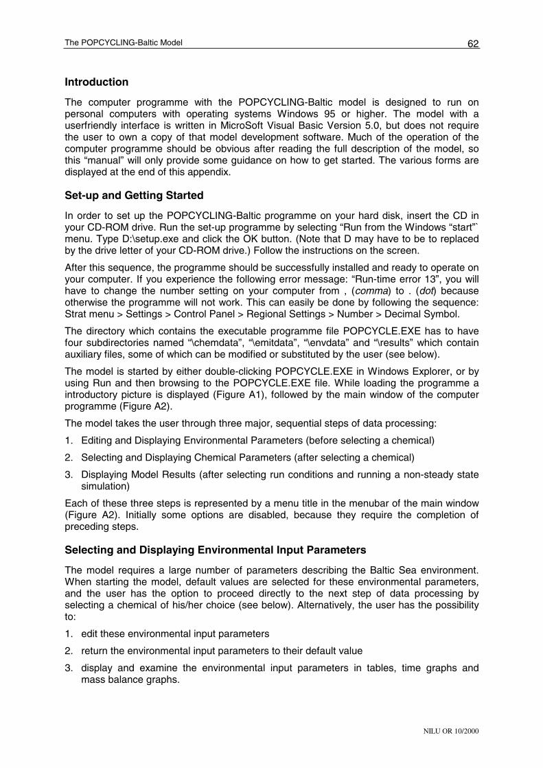
The POPCYCLING-Baltic Model
NILU OR 10/2000
62
Introduction
The computer programme with the POPCYCLING-Baltic model is designed to run on personal computers with operating systems Windows 95 or higher. The model with a userfriendly interface is written in MicroSoft Visual Basic Version 5.0, but does not require the user to own a copy of that model development software. Much of the operation of the computer programme should be obvious after reading the full description of the model, so this “manual” will only provide some guidance on how to get started. The various forms are displayed at the end of this appendix.
Set-up and Getting Started
In order to set up the POPCYCLING-Baltic programme on your hard disk, insert the CD in your CD-ROM drive. Run the set-up programme by selecting “Run from the Windows “start”` menu. Type D:\setup.exe and click the OK button. (Note that D may have to be to replaced by the drive letter of your CD-ROM drive.) Follow the instructions on the screen.
After this sequence, the programme should be successfully installed and ready to operate on your computer. If you experience the following error message: “Run-time error 13”, you will have to change the number setting on your computer from , (comma) to . (dot) because otherwise the programme will not work. This can easily be done by following the sequence: Strat menu > Settings > Control Panel > Regional Settings > Number > Decimal Symbol.
The directory which contains the executable programme file POPCYCLE.EXE has to have four subdirectories named “\chemdata”, “\emitdata”, “\envdata” and “\results” which contain auxiliary files, some of which can be modified or substituted by the user (see below).
The model is started by either double-clicking POPCYCLE.EXE in Windows Explorer, or by using Run and then browsing to the POPCYCLE.EXE file. While loading the programme a introductory picture is displayed (Figure A1), followed by the main window of the computer programme (Figure A2).
The model takes the user through three major, sequential steps of data processing:
1. Editing and Displaying Environmental Parameters (before selecting a chemical)
2. Selecting and Displaying Chemical Parameters (after selecting a chemical)
3. Displaying Model Results (after selecting run conditions and running a non-steady state simulation)
Each of these three steps is represented by a menu title in the menubar of the main window (Figure A2). Initially some options are disabled, because they require the completion of preceding steps.
Selecting and Displaying Environmental Input Parameters
The model requires a large number of parameters describing the Baltic Sea environment. When starting the model, default values are selected for these environmental parameters, and the user has the option to proceed directly to the next step of data processing by selecting a chemical of his/her choice (see below). Alternatively, the user has the possibility to:
1. edit these environmental input parameters
2. return the environmental input parameters to their default value
3. display and examine the environmental input parameters in tables, time graphs and mass balance graphs.

The POPCYCLING-Baltic Model
NILU OR 10/2000
63
Editing Environmental Input Parameters
The default parameters are believed to represent the best estimate of the real environmental conditions in the Baltic Sea environment. Nevertheless the user may wish to modify these default values, for example in order to test the sensitivity of a model result to a particular parameter, or if a better estimate becomes available. The procedure for editing environmental parameters is different for parameters which are fixed in time versus those which can fluctuate with season.
TIME-INVARIANT INPUT PARAMETERS
Four forms (Figure A3a-d) allow the user to change input parameters relating to (1) the atmospheric, (2) the terrestrial, and (3) the aqueous environment and (4) to the hydrology of the Baltic Sea environment. These forms are displayed by selecting one of the four first menu options in the menu called <Environmental Parameters>. The values are simply edited by typing a modified value in the respective textbox. The model does NOT perform a check of the reasonability of the selected value, and it is the responsibility of the user to assure consistent and sensible parameter choices. Changes to the input parameters can not be stored permanently and upon restarting the programme, the parameters are returned to their default values. The forms can display only the values for one of the various regions at a time. To display and edit values for other regions, select that region using the respective drop-down menu.
TIME-VARIANT INPUT PARAMETERS
A number of environmental input parameters are functions of time, namely temperature, wind speed, atmospheric hydroxyl radical concentrations and atmospheric advection rates. These data are read as monthly values from files upon starting the computer programme and can not be edited as readily as the parameters which are fixed in time. Namely, in order to edit these parameters the user has to open and edit the respective data files prior to starting the programme. These files, which are located in subdirectory “\envdata”, are:
TKA.txt, TKT.txt, TKC.txt, TKO.txt
WST.txt, WSC.txt, WSO.txt
OHconc.txt
Advection.txt
All these files are in ASCI format and can for example be edited in NOTEPAD. When editing these files, it is important that the location, name and the formatting of the files stays the same. It is recommended that the user makes copies of the orignal data files before making changes.
All of these files contain 12 lines with values for each month, starting with January in the first line. TKA.txt and OHconc.txt each have four entries per line (6 and 7 digits respectively, without delimiter), pertaining to the atmospheric temperature in K and the OH radical concentration in molecules per cm3 in the four atmospheric compartments in the sequence North, East, South, West. The files TKC.txt, TKT.txt, WSC.txt and WST.txt have 10 entries per line (6 digits for TKX, 4 digits for WSX, no delimiters), pertaining to the surface temperature in K and the wind speed in m/s for the coastal and terrestrial units of the model. The sequence in each case is: Bothnian Bay, Bothnian Sea, Gulf of Finland, Neva, Gulf of Riga, Southern Baltic Proper, Swedish Baltic Proper, Danish Straits, Kattegat, Skagerrak. The files TKO.txt and WSO.txt provide the analogous data for the open water units. There are six 6-digit entries for TKO, but only five 4-digit entires for WKO, because no wind speeds apply to the bottom water compartment. The sequence of the entires is: Bothnian Bay, Bothnian Sea, Gulf of Finland, Baltic Proper surface water, (Baltic Proper bottom water,) Skagerrak. Finally, in the file Advection.txt each of the 12 lines has 16 nine-digit entries with

The POPCYCLING-Baltic Model
NILU OR 10/2000
64
the atmospheric advection rates in m2/day. The sequence is: N to E, E to N, E to S, S to E, S to W, W to S, W to N, N to W, N to O, O to N, E to O, O to E, S to O, O to S, W to O, O to W, where O stands for outside of the model region.
Returning Environmental Input Parameters to their Default Value
Time-invariant environmental parameters that have been edited in one of the four forms as described above can be returned to their default values by selecting the menu choice <Set to Defaults> under the menu option <Environmental Parameters>. They are automatically returned to their default value when the program is started again. A permanent change of the time-invariant parameters is only possibly in the source code.
Displaying Environmental Parameters in Tables, Time Graphs and Mass Balance Graphs
The forms displaying environmental parameters are called up by using various options under the menu option <Environmental Parameters>. These forms allow the user to inspect the effect of changing and editing environmental input parameters on the environmental parameters derived from these.
DISPLAYING SOME ATMOSPHERIC PARAMETERS
By selecting the heading <Display Atmospheric Parameters> a form (Figure A4) is displayed that allows the user to inspect the height, volumes, aerosol content, temperature, and air residence time for the four atmospheric compartments. Also, the atmospheric advection rates in km/h3 can be displayed. For the time-variant parameters it is possible to display the values for each day of the year. The days can be selected by either using the arrow buttons to flip from day to day, or by typing the Julian day in the textbox provided for this purpose, followed by a carriage return.
DISPLAYING SOME MARINE PARAMETERS
By selecting the heading <Display Marine Parameters> a form (Figure A5) is displayed that allows the user to inspect the dimensions (depth, surface area and volume) of the marine water and sediment compartments, the POC concentration, the temperature, and the water residence time in the marine water compartments. The water temperatures can be displayed for each day.
DISPLAYING SOME TERRESTRIAL PARAMETERS
By selecting the heading <Display Terrestrial Parameters> a form (Figure A6) is displayed that allows the user to inspect the dimensions (depth, surface area, volume) and temperatures of the terrestrial compartments, the organic carbon content or the soils and fresh water sediments, and the fresh water residence time. The temperatures can be displayed for each day.
DISPLAYING THE WATER BALANCE
Water fluxes in units of km3/a can be displayed in various form when selecting one of three options under the heading <Display Water Balance>. When selecting <in Table>, a table showing the various fluxes of the steady-state water balance for the drainage basin of the Baltic Sea is displayed (Figure A7). When selecting <in Overview Graph>, a graph showing the water fluxes between the 16 marine compartments of the model, as well as the precipitation, evaporation and riverine water fluxes for each of these basins, is displayed (Figure A8). Finally, when selecting <in Basin Graphs>, a graph is displayed which shows the water fluxes in one of the ten terrestrial/coastal units (Figure A9). Use the dropdown menu to select the basin for which you wish these fluxes shown.

The POPCYCLING-Baltic Model
NILU OR 10/2000
65
DISPLAYING THE POC BALANCE
Graphs of the fluxes of particulate organic carbon in the various aquatic systems are displayed upon selecting <Display POC Balance> and <in Basin Graphs>. Choose the freshwater/coastal unit or open water basin for which you wish the fluxes displayed by selecting the respective menu choice. Depending on the choice of aquatic system, three different types of graphs are displayed (Figure A10a-c). By clicking the respective option box, the POC fluxes are either shown in units of kt/year or as area-normalised fluxes in units of g/(m2· a). An overview graph similar to that for water (Figure A8) showing the POC fluxes between the marine compartments in kt/year is displayed upon choosing <Display POC Balance> and <in Overview Graph>.
DISPLAYING TIME-VARIANT ENVIRONMENTAL PARAMETERS
The time variant environmental parameters can be displayed by selecting <Display Time Graphs> from the menu entitled <Environmental Parameters>. Upon selecting one of the menu options provided the environmental parameters are displayed as a function of time for a one year period. Figure A11 gives an example. The following parameters can be displayed: Input parameters: temperature, windspeed, OH radical concentration, atmospheric advection rates. Derived parameters: Fresh water temperature, sea ice cover, atmospheric residence time, volume of forest cover, litter fall rate, dry particle deposition velocities and gaseous mass transfer coefficients to various surfaces.
Selecting and Displaying Chemical Parameters
Selecting Chemical Parameters
For performing the simulation the following physical-chemical properties for the substance of interest are required:
• Molecular mass in g/mol
• Two out of the following three dimensionless equilibrium partition coefficients:
Octanol-water partition coefficient log KOW
Air-water partition coefficient log KAW
Octanol-air partition coefficient log KOA
The third partition coefficient is calculated from the other two.
• Two out of the following three heats of phase transfer in units of J/mol:
Heat of phase transfer between octanol and water ∆HOW
Heat of phase transfer between air and water ∆HAW
Heat of phase transfer between air and octanol ∆HOA
The third heat of phase transfer is calculated from the other two.
• Degradation half lives at the reference temperature 25°C in hours in each of the environmental media. For the atmosphere the reaction rate of vapor phase chemical with OH radicals in cm³/(molecules· s) is required.
• Activation energies (i.e. temperature dependence slopes) for these degradation reactions in J/mol.
To facilitate that task, the model contains a database which allows the user to retrieve and store these data for a large set of chemicals. Access to this database is provided through a form (Figure A12) that is displayed upon choosing <Input Chemical Properties> from the menu named <Chemical Properties>. On this form the user can (1) use the chemical properties provided for a number of chemicals by selecting the respective choice in the drop-

The POPCYCLING-Baltic Model
NILU OR 10/2000
66
down menu, (2) modify these chemical properties temporarily by editing the data displayed in the text boxes, or (3) permanently store modified or entirely new chemical property profiles in the database. It should be self-explanatory how that is done. By clicking the <OK> button on that form, the user accepts the values displayed in the text boxes for use in the simulation.
When choosing chemical properties, it is imperative to keep in mind that this model was developed for persistent organic pollutants, i.e. a fairly select group of chemicals that are highly apolar, persistent and have intermediate volatility. In particular, the model relies on a several empirical regressions that relate the partitioning between water and natural organic matter in soils, sediments and suspended solids with that between water and octanol (Seth et al., 1999), and that between air and atmospheric aerosols and between air and vegetation with that between air and octanol (Finizio et al., 1996, Horstmann and McLachlan, 1998). The model should thus only be used for substances for which these empirical relationships are valid. Also, the model is unsuitable for very short-lived chemical species for which the assumption of homogeneity within fairly large areas, which is inherent in compartmental box models, does not apply.
In addition to the chemical properties, the fate of a chemical is influenced by some emission related parameters, namely the mode of emission, i.e. the compartment(s) into which the chemical is being release/discharged, and the seasonal variability of the discharge. Since these parameters are often different for different chemicals, they are stored together with the true chemical property parameters in the chemical property database. These are default values which can be modified for each of the 10 individual terrestrial region (see below).
Displaying Chemical Parameters
Upon making a selection for the chemical properties, the menu choice <Display Time Graphs> from the menu named <Chemical Properties> becomes enabled. Clicking this menu option, opens a window (Figure A13) that allows the display of time-dependent chemical properties over a one year period similar to the graphs discussed above for the environmental parameters (Figure A11). In fact, the environmental parameters are included among the menu options of that window. The time variant chemical parameters that can be displayed this way, are the partition coefficients between octanol and air and between water and air at various model temperatures, the degradation half-lives and rates in all compartments, the bulk Z-values and the products of the bulk Z-values and compartment volumes, and the D-values.
Performing a Simulation
With environmental and chemical properties being specified, additional information is required before a simulation can be performed, namely a emission scenario has to be specified, and the simulation conditions such as simulation period, step size and results storage intervals have to be specified.
Specifying a Emission Scenario and Boundary Conditions
Upon making a selection for the chemical properties, the menu choice <Input Emission Parameters> from the menu named <Chemical Properties> becomes enabled, and allows to call up a form (Figure A14) to specify the emission scenario.
READING FILE WITH ANNUAL NATIONAL EMISSION RATES AND BOUNDARY CONDITIONS
Annual emission rates in tons and fugacity ratios defining the boundary conditions are read from a file. This is done by pressing the button called <Select File>, browsing for, and selecting the name of an emission file, and pressing the <OK> button.

The POPCYCLING-Baltic Model
NILU OR 10/2000
67
Presupplied emission files for the chemicals α-HCH, γ-HCH and PCBs are located in the subdirectory entitled “emitdata”. These files can also be constructed by the user, but they have to be ASCI files with a prescribed format. The first line contains four digits indicating the number of years for which emission rates and fugacity ratios are supplied, e.g. 0070. The second line contains four digits indicating the first year for which emission rates and fugacity ratios are supplied, e.g. 1930. Then follow as many lines as have been specified in the first line. All these lines have 18 nine digit entries (without delimiters) applying to a particular year.
• The first thirteen entries give the emission rate in t/a into the thirteen countries with a share of the Baltic Sea drainage basin (in the sequence Belorus, Czech and Slovak Republics, Denmark, Estonia, Finland, Germany, Latvia, Lithuania, Norway, Poland, Russia, and Sweden, Ukraine)
• the next four entries give the ratios between the inflowing and outflowing air fugacity for the four atmospheric compartments (in the sequence: North, East, South, West).
• the last entry gives the ratio between the fugacity in water inflowing from the North Sea and the fugacity of the water flowing out of the Skagerrak.
SPECIFYING OTHER PARAMETERS RELATED TO THE EMISSION SCENARIO
On the same form a number of parameters related to the emission scenario have to be specified.
1. It has to specified how the national release rates are to be spatially distributed to calculate the release rates for the ten drainage basins. Three options are provided: spatial assignment based on crop area, based on population, or based on a combination of the two. If the latter option is selected, the fraction assigned based on population is to be entered for each country.
2. For each drainage basin, the following information is required:
Scaling factor: a fixed multiplication factor scaling the emission rates. This factor is meant to help modelling individual constituents of chemical mixtures for which only composite emission data are available. The scaling factor then is the fraction of the total release that applies to a constituent, e.g. the fraction of a single congener in a PCB mixture.
Seasonality of the release: The total annual release can be distributed over the year using a sinusoidal function. The amplitude of the seasonal fluctuation has to be specified as a fraction of the annual mean. An amplitude of “0” means no seasonal variability, whereas an amplitude of “1” implies the maximum possible variability. Additionally, the month during which maximum release occurs needs to be specified.
Mode of emission: the compartmental distribution of the emissions is defined by giving fractions of the total release which are entering a certain compartment. These fractions obviously have to add up to 1 within each drainage basin.
Defaults for the latter two are already selected with the chemical property database, but can now be modified for individual terrestrial regions. The form displays only the values for one of the ten regions at a time. To display and edit values for other regions, select that region using the respective drop-down menu. The default options are a scaling factor of 1, no seasonal fluctuation, and release into the air compartment only.
Specifying the Simulation Conditions and Performing the Simulations
When the emission scenario has been accepted, a frame which allows the specification of the simulation conditions appears on the main window (Figure A15). Namely, the following parameters are required to perform a non-steady state simulation:

The POPCYCLING-Baltic Model
NILU OR 10/2000
68
Date when simulation starts: This date can not be changed. For the first simulation it has to be the year when emissions started. This year has been specified in the second line of the emissions file (see above). Every first simulation starts on a January 1.
Date when simulation ends: The length of the simulation is controlled by selecting the date when the simulation should stop. That date is to be entered into the respective textbox as a year. Obviously the number has to larger than the starting date. The simulation length does not have to be a multiple of full years, but the date when the simulation ends could also be an uneven number, e.g. “1995.3”. The default ending date is the last year for which emission data have been read from file.
Time Step for Simulation: The default time step used for the step-size numerical solution is 12 hours. The user may specify a smaller or higher step size among the provided options (1, 3, 6 and 24 hours). A step size smaller than 12 results in increased calculation times, but usually provides only marginal reductions in the numerical errors, if any.
Time Step for Results Storage: After certain predefined intervals during the simulation, the calculated fugacities in all model compartments are stored for later retrieval and processing. The user can specify this interval from among the choices provided (24 h, 120 h, 1752 h, 8760 h). The selection of that parameter affects for how the model results can be displayed. A shorter storage interval provides high temporal resolution, but time graphs can only be displayed for fairly short simulation times. A larger storage interval results in a loss of temporal resolution, namely on seasonal or shorter time scale, but allows the plotting of time curves over several decades. To display the results in graphical form, there needs to be a minimum of 2 storage events.
The simulation is started by clicking the button <Start Numerical Solution>. The progress of the numerical solution is displayed in a window until the simulation has been completed (Figure A16). Then the menu choice <Simulation Results> will become enabled. Note that if the environmental or chemical parameters are changed after a simulation has been performed, this menu choice <Simulation Results> becomes disabled again. This reflects the fact that the simulation has to be repeated with changed input conditions to look at the results.
After the first simulation is completed, the user has two options:
• Continue the simulation by clicking the option button <End of last simulation> in the frame entitled <Initial Fugacities> and then entering a new date when simulation should end. The year when simulation starts is automatically updated. The continuation can have simulation parameters (step size, results storage interval, etc.) that differ from those used in the initial part of the simulation. A simulation can be continued several times.
• Conduct a new simulation starting in the year the emission started.
Please note that whenever a new simulation is started or a simulation is continued, the stored results from the previous simulation are lost.
Displaying Model Results
The programme provides a multitude of ways to display the simulation results. As mentioned above during the simulation the fugacities in all model compartments are stored at user-defined intervals. Naturally, it is only possible to display results for these storage events. When results other than fugacities are being displayed, these are calculated from the stored fugacities values.
In addition to these instantaneous results, the model calculates cumulative fluxes, i.e. it sums up the rates and fluxes for the entire simulation period. Please note that if the
The POPCYCLING-Baltic Model
NILU OR 10/2000
69
simulation is a continuation of a previous simulation, these cumulative fluxes only refer to the last part of the simulation.
The results display options are accessible through various menu options under the main menu title <Simulation Results>.
Displaying the Simulation Results in Tables
Menu choice <Display Tables> opens a window, on which the values of selected parameters at the storage events can be displayed in a table (Figure A17).
Displaying the Simulation Results as Time Graphs
Menu choice <Display Time Response> opens a window (Figure A18) that allows the display of many model parameters as a function of time for the simulation period. Please note that if the simulation is a continuation of a previous simulation, these graphs show only the last part of the simulation. The temporal resolution of the graphs is obviously determined by the chosen storage interval (see above). The parameters that can be displayed are: fugacities, fugacity ratios, concentrations, amounts, fluxes and rates, net fluxes. The graphs can be printed in various form.
Displaying Fluxes in Overview Graphs
The form that displayed the fluxes of water and POC between the marine compartments in the whole Baltic Sea in an overview graph (Figure A8), can now be used to display advection D-values, instanteneous and cumulative chemical fluxes between these marine water compartments. The window is displayed upon selecting the menu choice <Display Marine Fluxes>.
Displaying Fluxes in the Terrestrial/Coastal Systems
When selecting the menu choice <Display Terrestrial/Coastal Fluxes>, a window appears that displays mass balances of water and chemical within the ten terrestrial/coastal units of the Baltic Sea environment model (Figure A19). The fluxes can be displayed for each stored event, and as cumulative fluxes. They also can be shown as area-normalised fluxes. Please note that the atmospheric compartments are larger than the terrestrial/coastal units of these graphs. The advection, degradation and emission rates to the atmosphere which are displayed on these graphs have been scaled to the size of the terrestrial/coastal units.
Displaying Graphs With Atmospheric, Marine and Terrestrial Results
Three windows display maps allowing the direct comparison between the results for various atmospheric, marine and terrestrial regions. These are displayed by choosing the menu options <Display Atmospheric Results>, <Display Marine Results>, and <Display Terrestrial Results> and are similar to those showing environmental parameters (Figure A4 to A6). However, additional menu options allow the display of fugacities, concentrations, amounts, D-values, fluxes and rates, and cumulative fluxes.
Writing Results to File
The results (fugacities and concentrations) can also be written to ASCI files for further processing. Selecting menu option <Write Results To Files> displays a windows (Figure A20), that allows to choose which parameters to write to ASCI files (by clicking the respective checkmarks), and what names these files should have (by writing the respective names into the textboxes provided). By clicking the buttons <Write to File> the files will be saved in the subdirectory “\results”.

The POPCYCLING-Baltic Model
NILU OR 10/2000
70
The files have one line for each storage event. The number of lines is thus determined by both simulation length and time step for results storage. Only the data for the last simulation (in the case of a continued simulation only the results for the last section of the simulation) will be saved to file. The first entry of each line gives the simulation time in hours (with respect to the year when emissions first started), the following entries are the respective concentrations or fugacities. The entries are delimited by commas. The first line in each file provides information on the content of the file and the units used for the concentration values. The second line indicates to which region the values refer. The files can be opened in spreadsheet programmes such MS Excel for further processing.
The programme is closed by clicking the menu option <Exit>.
Figure A1

The POPCYCLING-Baltic Model
NILU OR 10/2000
71
Figure A2
Figure A3a
Figure A3b

The POPCYCLING-Baltic Model
NILU OR 10/2000
72
Figure A3c
Figure A3d

The POPCYCLING-Baltic Model
NILU OR 10/2000
73
Figure A4 Figure A5

The POPCYCLING-Baltic Model
NILU OR 10/2000
74
Figure A6 Figure A7

The POPCYCLING-Baltic Model
NILU OR 10/2000
75
Figure A8
Figure A9

The POPCYCLING-Baltic Model
NILU OR 10/2000
76
Figure A10a
Figure A10b
Figure A10c

The POPCYCLING-Baltic Model
NILU OR 10/2000
77
Figure A11
Figure A12

The POPCYCLING-Baltic Model
NILU OR 10/2000
78
Figure A13
Figure A14

The POPCYCLING-Baltic Model
NILU OR 10/2000
79
Figure A15
Figure A16

The POPCYCLING-Baltic Model
NILU OR 10/2000
80
Figure A17
Figure A18

The POPCYCLING-Baltic Model
NILU OR 10/2000
81
Figure A19
Figure A20

Norwegian Institute for Air Research (NILU) P.O. Box 100, N-2027 Kjeller, Norway
REPORT SERIES
SCIENTIFIC REPORT
REPORT NO. OR 10/2000
ISBN 82-425-1159-4
ISSN 0807-7207
DATE SIGN. NO. OF PAGES
81
PRICE
NOK 285,-
TITLE
The POPCYCLING-Baltic Model
PROJECT LEADER
Frank Wania
A non-steady state multicompartment mass balance model of the fate of persistent organic pollutants in the Baltic Sea environment.
NILU PROJECT NO.
U-96069
AUTHOR(S)
Frank Wania1, Johan Persson2, Antonio Di Guardo3, Michael S. McLachlan4,
CLASSIFICATION *
A
CONTRACT REF.
Jozef M. Pacyna REPORT PREPARED FOR Norwegian Institute for Air Research, NILU P.O. Box 100 N-2027 KJELLER
ABSTRACT The POPCYCLING-Baltic model, typical multi-media mass balance model, divides the environment in 85 boxes or compartments, which are considered well-mixed and homogeneous, both with respect to the environmental characteristics and chemical contamination. These environmental phases are then linked by a variety of intercompartmental transfer processes.
NORWEGIAN TITLE
POPCYCLING-Baltic modellen
En dynamisk massebalansemodell som beskriver omsetningsforhold for organiske miljøgifter i Østersjøregionen.
KEYWORDS
POP
Cycling model
The Baltic ABSTRACT (in Norwegian) Popcycling-Baltic modellen ble utviklet under kontrakt for NILU som en del av EU-prosjektet "Popcycling-Baltic" (ENV4-CT96-0214). Modellen som er beskrevet i denne rapporten er en fugasitets-basert dynamisk massebalansemodell. Østersjøregionen er representert i modellen med 85 ulike bokser for terrestrisk, akvatisk og atmsossfærisk miljø. * Classification A
B C
Unclassified (can be ordered from NILU) Restricted distribution Classified (not to be distributed)