THE POWER OF FEEDBACK

FEEDBACK CONTROL

Let’s return to the problem of controlling the output y(t)

of a dynamical system in spite of disturbances d(t) using

the control signal u(t)

--

?

S yu

d

Assume that the system is described by

dy(t)

dt+ ay(t) = bu(t) + cd(t)

Our goal is keep the controlled output y(t) close to a

desired value r,

y(t) ≈ r

despite the effect of the disturbance d(t)

r: setpoint for y(t) (s. borvarde, fi. asetusarvo)

2

At first sight, using a purely static analysis and ignoring

the dynamic system behavior by setting dy(t)/dt = 0, it

would seem to make sense to cancel the effect of d(t) and

setting y(t) = r by selecting u(t) so that

ar = bu(t) + cd(t)

or

u(t) = −a

b[ar − cd(t)]

Then the transient, dynamic, behavior of the system is

then described by

dy(t)

dt+ ay(t) = ar

Comments:

• Method requires that the disturbance d(t) is known

(wind, friction, etc). This is impossible in practice!

• Method requires that system model is known, as can-

celing the effect of disturbance requires knowledge of

parameters a, b, c (which depend on mass of car, air

drag coefficient etc.). In practice knowledge of system

parameters is always more or less inexact.

• The dynamic response determined by parameter a

has not been affected. If a is small the response would

be very slow, and worse, if a < 0 the system would

even be unstable!

3

We need a better approach!

When manually driving a car, we use the current speed to

adjust the engine power, or the current course and road

direction for steering a car in the correct direction.

In other words:

We should use feedback from the signal we wish to

control!

4

Block diagram showing the connection between the vari-

ous signals and systems in feedback system:

?

d

Gcyuer Gp

6e+

−-- - -

Gp: system to be controlled

Gc: the controller

e(t) = r − y(t): control error

5

Let’s try to control the first-order system

dy(t)

dt+ ay(t) = bu(t) + cd(t)

using feedback from the measured output y(t).

Take the simple linear control law

u(t) = Kp [r − y(t)] (1)

where u(t) is proportional to the control error e(t) =

r − y(t).

Then the controlled system is described by

dy(t)

dt+ (a + bKp) y(t) = bKpr + cd(t)

Observations:

• For a constant disturbance d(t) = d0, we have

y(t) → bKp

a + bKpr +

c

a + bKpd as t → ∞

Hence for a sufficiently large Kp such that Kpb > 0

we havebKp

a + bKp≈ 1,

c

a + bKp≈ 0

and hence we have approximately y(t) → r.

• The transient response is determined by

a + bKp

and can be made faster by selecting a large Kp.

6

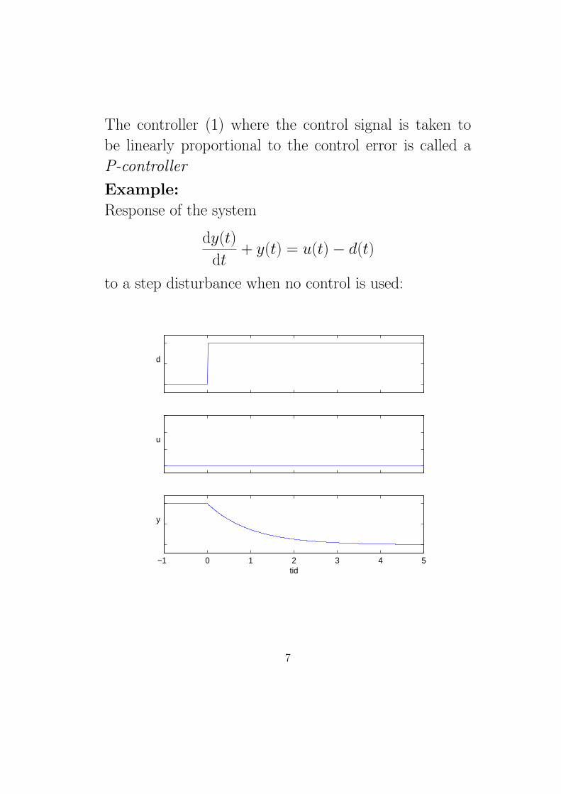
The controller (1) where the control signal is taken to

be linearly proportional to the control error is called a

P-controller

Example:

Response of the system

dy(t)

dt+ y(t) = u(t)− d(t)

to a step disturbance when no control is used:

d

u

−1 0 1 2 3 4 5

y

tid

7

Response when using the control law

u(t) = Kp (r − y(t)) , Kp = 2

d

u

−1 0 1 2 3 4 5

y

tid

8

We see that by using feedback the effect of the disturban-

ce can been reduced:

- without the need to know the disturbance

- without knowing exact values of the system parameters

Limitations of P-controller:

- only one design parameter, Kp by which the response

can be affected

- complete cancellation of constant step disturbance requires

infinite gain Kp

These limitations can be overcome by using a controller

which integrates the control error. This gives the

I-controller:

u(t) = Ki

∫ t

τ=0(r − y(τ )) dτ

Idea:

As long as y(t) < r, the integral grows, and hence u(t)

is increased/decreased until y(t) = r, and vice versa,

as long as y(t) > r, the integral reduces, and hence u(t)

is decreased/increased until y(t) = r.

9

Example:

Using the I-controller for previous example

(Ki = 5)

d

u

−1 0 1 2 3 4 5

y

tid

The I-controller cancels the effect of an unknown constant

step disturbance by an adaptation mechanism (u(t) is

adjusted as long as y(t) = r)

10

Limitations of I-controller:

- the controller still has only one design parameter, Ki,

by which the response can be affected

- response may be sluggish, as it takes some time for the

integral to grow or decrease

- the slow change of the integral may lead to oscillatory

response (cf. figure)

These limitations can be overcome by combining the P-

and I-controllers. This gives the

PI-controller:

u(t) = Kp [r − y(t)] +Ki

∫ t

τ=0(r − y(τ )) dτ

Idea:

The proportional (P) component gives a fast response

when y(t) = r, and the integrating (I) component cancels

the effect of unknown step disturbances

11

Example:

Using the PI-controller for previous example

(Kp = 2, Ki = 5)

d

u

−1 0 1 2 3 4 5

y

tid

The PI-controller gives a faster response than the I-controller

without oscillations, and cancels effect of constant distur-

bance

12

Limitations of PI-controller:

- the controller still has only two design parameters, Kp

and Ki, by which the response can be affected. Alt-

hough better than only one parameter, this still limits

how the response can be affected

- the controller reacts only when y(t) = r, i.e., after there

is a control error

The response can be made still faster by introducing a

derivative (D) component. This gives the

PID-controller:

u(t) = Kp [r−y(t)]+Ki

∫ t

τ=0(r − y(τ )) dτ+Kd

d(r − y(t))

dt

Idea:

The derivative (D) component reacts already to the rate

of change in the control error even before any error exists,

resulting in a faster response

13

Example:

Using the PID-controller for previous example

(Kp = 2, Ki = 5, Kd = 0.5)

d

u

−1 0 1 2 3 4 5

y

tid

Controller reacts instantaneously when dy(t)/dt = 0,

resulting in faster response.

14

Limitation of PID-controller:

- Derivation is sensitive to noise, and in practice it can

therefore not be applied in pure form

- Derivative action in a controller would lead to sudden

step changes in control signal (cf. above figure), which

would result in excessive wear of equipment

Remedy:

Instead of taking the time derivative of the output y(t)

directly, we filter it first. A common method is to modify

the PID-controller as follows:

u(t) = Kp [r − y(t)] +Ki

∫ t

τ=0(r − y(τ )) dτ +Kd

dx(t)

dt

where x(t) is obtained by filtering the control error ac-

cording to

dx(t)

dt+ aix(t) = bi (r − y(t))

15

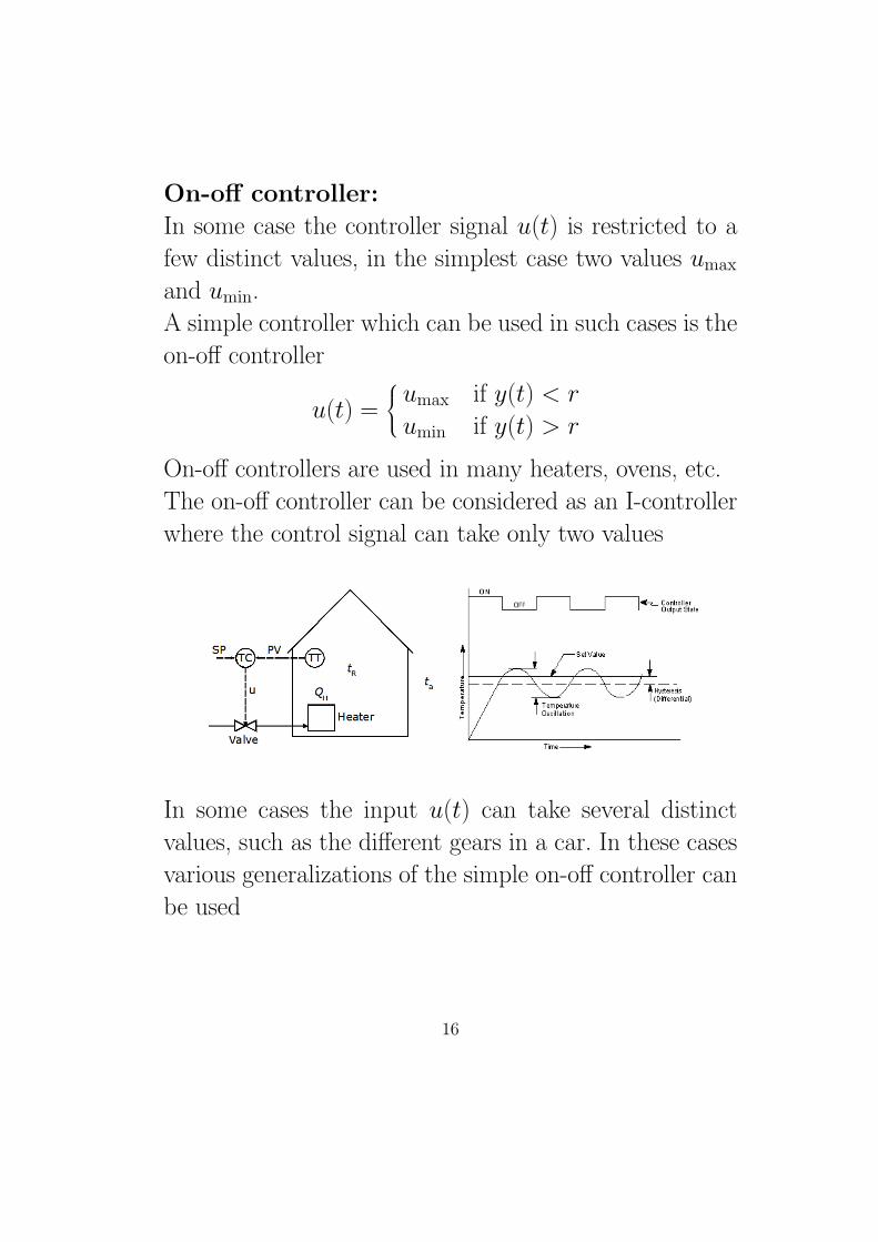
On-off controller:

In some case the controller signal u(t) is restricted to a

few distinct values, in the simplest case two values umax

and umin.

A simple controller which can be used in such cases is the

on-off controller

u(t) =

umax if y(t) < r

umin if y(t) > r

On-off controllers are used in many heaters, ovens, etc.

The on-off controller can be considered as an I-controller

where the control signal can take only two values

In some cases the input u(t) can take several distinct

values, such as the different gears in a car. In these cases

various generalizations of the simple on-off controller can

be used

16

In spite of their simplicity, the P-, PI- and PID-controllers

are quite powerful, and for systems with a not-too-complex

dynamics they are the most commonly used controller

structures used in practice.

For practical work, a number of tuning rules to select

the controller parameters Kp, Ki and Kd have been de-

veloped. Of course, in order to tune a controller some

knowledge of the system dynamics must be available.

These simple controllers are, however, not sufficient for

systems with

• complex dynamic behaviour,

• most unstable systems,

• systems with many outputs to be controlled, and ma-

ny control inputs

There is a vast, and in many cases quite advanced, theory

of how to design controllers for all kinds of dynamical

systems.

17

Feedforward

In spite of the power of pure feedback from measured

system outputs, it still makes sense to use measurements

of disturbances as well when these are available. This is

called feedforward (s. framkoppling, fi. myotakytkenta)

control

?

d

Gcyuer Gp

Gf�

?e6e+

−-- -- -

18

Example:

in controlling the temperature in a building, the indo-

or temperature (controlled signal) is used for feedback,

whereas the outdoor temperature (disturbance) is used

for feedforward

We have the following control methods:

• In open-loop control, no measurement are used to

determine the control signal P .

• In pure feedback control, the control signal P is a

function of the controlled signal T only.

• In pure feedforward control, the control signal P is

a function of the disturbance signal Ty only.

• In combined feedback and feedforward control, the

control signal P is a function of both the controlled

signal T and the disturbance signal Ty.

19

Uses of feedback control

Feedback control can be applied in several ways:

• Servo control.

To control a system in such a way that y(t) follows

a given trajectory r(t) despite (unknown) disturban-

ces and (often) incomplete knowledge of the system

dynamics.

Examples: driving a car along a road, controlling mo-

vement of robot arm from one position to another.

20

• Regulator problem.

To control a system in such a way that y(t) is as close

to the setpoint r as possible despite disturbances.

The simulation examples above have all been regu-

lator problems, where the disturbance has been an

step disturbance.

Often the disturbance has the character of random

noise. Then the control objective is to minimize the

variance of the control error, E[(y(t)− r)2

].

This problem is important in statistical process con-

trol, where the objective is to make a high-quality

product, such as paper with constant thickness and

other properties.

21

Example of reducing the output variance.

0 100 200 300 400 500 600 700 800 900 1000−20

−15

−10

−5

0

5

10

y(t)

Without control

0 100 200 300 400 500 600 700 800 900 1000−20

−15

−10

−5

0

5

10

Time

y(t)

Minimum variance control

Above: without control

Below: using a controller which minimizes the output va-

riance

22

• Stabilization problem.

Feedback may be applied simply to stabilize an ot-

herwise unstable system, such as an exothermic che-

mical reactor, an airplane, a helicopter, an inverted

pendulum, or an unstable vehicle.

23

• To change system dynamics.

Feedback can be used to change the dynamical pro-

perties of a system, for example to make it easier

maneuverable for a human. For example,

- modern supersonic airplanes react rapidly and have

dynamic properties which make them difficult or

impossible to control manually. By changing the

dynamics with feedback control manual control

is possible.

- in precision instruments, such as electron microsco-

pes, telescopes, or robotic surgery accurate po-

sition of the instrument is made by a feedback

controller, although the desired position is deter-

mined manually.

24

Observe that these cases can be considered as servo

problems, where the reference signal r(t) is determi-

ned manually.

25

SOME EARLY EXAMPLES OF FEEDBACK CONTROL

Before the use of electrical circuits, feedback control had

to be implemented by mechanical constructions.

Various mechanical designs based on feedback to control

liquid levels and flows have been used early on.

26

Mechanical methods for level control have been used from

ancient times.

And are useful even today:

The controlled variable (water level) is used to determine

the control variable (valve). This is an on-off feedback

controller, as the control variable can have only two states

(open-closed).

27

Watt’s centrifugal speed governor (1788) was used to con-

trol the speed of steam engines:

The controlled variable (rotation speed) is used to de-

termine the control variable (valve that determines the

steam flow.

28

As long as controllers had to be implemented by me-

chanical constructions, many processes were controlled

manually. The possibilities offered by electrical circuits

and, later, digital techniques, have made it possible to

solve and implement more demanding control problems

in practice.

29