the price effects of cross‐market mergers: theory and
TRANSCRIPT

RAND Journal of EconomicsVol. 50, No. 2, Summer 2019pp. 286–325
The price effects of cross-market mergers:theory and evidence from the hospitalindustry
Leemore Dafny∗Kate Ho∗∗and
Robin S. Lee∗
We consider the effect of mergers between firms whose products are not viewed as direct sub-stitutes for the same good or service, but are bundled by a common intermediary. Focusing onhospital mergers across distinct geographic markets, we show that such combinations can reducecompetition among merging hospitals for inclusion in insurers’ networks, leading to higher prices(or lower-quality care). Using data on hospital mergers from 1996–2012, we find support thatthis mechanism operates within state boundaries: cross-market, within-state hospital mergersyield price increases of 7%–9 % for acquiring hospitals, whereas out-of-state acquisitions do notyield significant increases.
1. Introduction
� Merger analysis is a staple of antitrust enforcement. When a merger eliminates current orpotential competition for a relevant product or service, enforcers may sue to block or unwind thetransaction. According to the most recent release of the “Horizontal Merger Guidelines,” whicharticulate the principles followed by the federal antitrust enforcement agencies, merger analysisis a “fact-specific process,” one in which the particulars of the relevant market(s) and mergingparties are integral to enforcement decisions. One such particular is the presence (or absence)of intermediaries in the chain of production or distribution. In this study, we evaluate mergersof upstream suppliers to intermediaries that bundle products or services for sale to customers,who in turn may aggregate the preferences of multiple individuals. We argue that the presence ofintermediaries selling to such customers can affect both the likelihood and margin of harm from
∗ Harvard University and NBER; [email protected], [email protected].∗∗ Princeton University, NBER, and CEPR; [email protected] thank the Editor, three anonymous referees, David Balan, Cory Capps, David Dranove, Gautam Gowrisankaran, AvivNevo, Bob Town, Nathan Wilson, and numerous conference and seminar participants for useful comments and discussion;and Matthew Schmitt and Victoria Marone for exceptional research assistance. All errors are our own.
286 C© 2019, The RAND Corporation.
DAFNY, HO AND LEE / 287
a merger of suppliers, and that harm to consumers may result, even if the products being suppliedare not direct “head-to-head” rivals at the point of sale. Examples of such settings include: cableTV, where different content producers offer channels that are not direct substitutes but negotiateprices with distributors that market a bundle of channels to multiperson households; and retailproduct markets, where products may be targeted to different consumers but are stocked byretailers offering one-stop shopping.
Health insurance is another relevant example. Private (commercial) insurers bargain withproviders (e.g., physicians or hospitals) over reimbursement rates (prices); the insurers then bundlethese services, adding in administrative and oversight features—as well as risk-bearing in the caseof “full insurance” products—and sell insurance plans to employers and households. Hospitals arecritical upstream suppliers to health plans, accounting for nearly one third of healthcare spendingin the United States today.1 In recent years, the Federal Trade Commission (FTC) has successfullychallenged several proposed mergers of hospitals that are direct substitutes at the point of care(i.e., in the same geographic and product market), informed by an economic literature showingthat these “within-market” mergers tend to result in price increases for privately insured patientswithout significant quality improvements.2
In contrast, there has been very little regulatory activity regarding hospital mergers acrossdistinct markets. This gap is notable in light of the significant pace of such “cross-market” mergersin recent years.3 More than half of the 528 general acute-care hospital mergers between 2000 and2012 involved hospitals or systems without facilities in the same CBSA,4 and a recent study byLewis and Pflum (2016) shows substantial increases in prices for independent hospitals acquiredby out-of-market systems (located 45+ minutes away), as well as price increases by nearby rivals.As we describe below, current methods of assessing the anticompetitive threat from hospitalmergers assume there can be no increase in bargaining leverage unless the merging parties arevying to provide the same set of services to the same set of patients. These methods implicitlyassume that insurance markets do not impact upstream market power; more formally, the modelstypically assume insurers face demand that is separable across product and service markets (asin Capps, Dranove, and Satterthwaite, 2003).
We argue that an extension to the current methodology is warranted in light of the role andrealities of intermediary markets. Insurers negotiate with and pay hospitals for their services,and demand for insurance may not, in fact, be separable across service markets. We show thatthe presence of “common customers” (e.g., employers or households) who purchase insuranceproducts and value the services offered by both merging parties can give rise to greater post-merger bargaining leverage for the merging hospitals, even when those hospitals operate in distinctpatient markets. These common customers are likely to be large employers that demand insuranceproducts covering hospital services in multiple distinct geographic markets, that is, areas wheretheir employees live and work. Because insurers serve employers in multiple geographic regions, amerged cross-market hospital system that covers those regions can demand higher reimbursementrates from insurers.5
1 CMS National Health Expenditure Accounts, available at www.cms.gov/research-statistics-data-and-systems/statistics-trends-and-reports/nationalhealthexpenddata/nhe-fact-sheet.html.
2 See Dranove and White (1994); Town and Vistnes (2001); Capps, Dranove, and Satterthwaite (2003); Gaynor andVogt (2003); Dafny (2009); Haas-Wilson and Garmon (2011); Farrell et al. (2011); Gaynor and Town (2012); Gaynor,Ho, and Town (2015), among others.
3 Examples include the $3.9 billion acquisition of Health Management (71 hospitals) by Community Health Systems(135 hospitals) in 2014, and the 2013 merger of Dallas-based Baylor Health Care System and Temple-based Scott &White Health; post-merger, the combined entity comprised 43 hospitals and more than 6000 affiliated physicians.
4 Data from Irving Levin on 528 general acute-care hospital mergers between 2000–2012 indicate that 256 (48.5%)involved hospitals located within the same CBSA; 193 (36.6%) were in the same state but not the same CBSA; whereas79 (15%) were out-of-state. A CBSA is defined as a metropolitan statistical area in larger cities, and a “micropolitan”area in smaller towns. For further details, see www.census.gov/programs-surveys/metro-micro/about.html.
5 Common customers for insurance products can also be households that demand services of hospitals in the samegeographic area but different product markets, for example, pediatric and cardiac specialty hospitals.
C© The RAND Corporation 2019.

288 / THE RAND JOURNAL OF ECONOMICS
Consider for illustrative purposes a simple setting where a state-wide employer choosesinsurance products to offer to employees who are evenly distributed across the state. Assumethere are 10 local markets, each of which contains three evenly sized, competing hospitals.Insurers engage in pair-wise bargaining with hospitals over prices. Under current antitrust practice,authorities would be likely to object to mergers of hospitals within a local market on the groundsthat they would “substantially lessen competition or tend to create a monopoly,” per Section7 of the Clayton Act.6 They would be unlikely, however, to object to cross-market mergers—even repeated mergers that created three large hospital systems, each owning a hospital in everymarket. However, the cross-market presence of the large employer implies a potentially largeeffect of these mergers on negotiated hospital prices. Although the employer would be unlikelyto drop an insurance plan that removed just one of the 30 hospitals from its network (because thiswould affect few of its employees), it would be much more likely to drop a plan that removed alarge hospital system representing a third of all hospitals. Thus, competition among insurers forinclusion in employers’ plan menus provides the large hospital system with greater bargainingleverage than individual hospitals to negotiate higher prices, even if no two hospitals in the systemoperate in overlapping service markets.
The first part of this article uses a theoretical model of bargaining between upstream suppliersand downstream intermediaries to formalize the intuition outlined above. Building on the modelin Ho and Lee (2017), we show that a sufficient condition for a market power effect of anupstream merger between hospitals is that the insurer’s objective function, typically representedby its profits, is submodular in the set of upstream hospitals—that is, the value of a hospitalto an insurer is decreasing in the size of the insurer’s hospital network. This condition can besatisfied under standard formulations for consumer demand and insurer profits if the hospitalsare valued by a common customer, (e.g., employer or household) even if they operate in differentservice markets. Our model formalizes some of the arguments in Vistnes and Sarafidis (2013),which includes numerical examples illustrating how price effects may arise when employersrecruit employees from different geographic areas. We also provide conditions under which amerger between hospitals negotiating with a common insurer, even absent common customers, issufficient to generate a price effect.7
The second part of the article explores the predictions of our model using panel dataon hospital prices and system acquisitions, supplemented with data on local insurance marketshares. We examine two distinct samples of acute-care hospital mergers over the period 1996–2012, and compare the price trajectories of three groups of hospitals: (i) hospitals acquiring anew system member in the same state but not the same narrow geographic market (“adjacenttreatment hospitals”); (ii) hospitals acquiring a new system member out-of-state (“nonadjacenttreatment hospitals”); and (iii) hospitals that are not members of “target” (i.e., acquired) oracquiring systems. To minimize concerns about the exogeneity of which hospitals are partiesto transactions, we focus on hospitals that are likely to be “bystanders” rather than the driversof transactions. Our first sample of transactions comprises mergers investigated by the FTCdue to potential horizontal overlap among the merging parties. We argue that hospitals that aremembers of the merging systems but located outside the areas of concern likely fall into thebystander category. Our second sample makes use of a broader set of mergers, that is, we beginwith the set of all mergers involving at least one hospital system over the period 2002–2012. Welimit the treatment group in two ways: first, we exclude hospitals that are the “crown jewels” ofeach deal (so the remaining hospitals are likely to be bystanders to the transaction); second, weexclude hospitals that gain a system member within 30 minutes (or are located within 30 minutesof another hospital that experiences the same over a five year period spanning the transaction
6 Throughout this manuscript, we refer to “price effects,” but our theoretical and conceptual observations applyequally to other potential merger effects, such as effects on quality or innovation.
7 Depending on the precise mechanism, these effects may not arise from a diminution of competition among themerging entitites.
C© The RAND Corporation 2019.

DAFNY, HO AND LEE / 289
of interest). This exclusion is designed to screen out same-market mergers. We also estimatespecifications that remove target hospitals altogether and consider the effect of the merger onacquirers’ prices.
We find that prices for adjacent treatment hospitals increase by 7%–10% relative to con-trol hospitals. The estimates for nonadjacent treatment hospitals are small, generally negative,and statistically insignificant. Our results also show that acquirers are raising their own prices,suggesting that significant quality improvements (such as might arise for targets following atakeover) are unlikely to be the source of price increases. Additional analyses reveal that priceeffects are largest when the merging parties have hospitals in closer geographic proximity (i.e.,30–90 minutes’ drive from one another; hospitals less than 30 minutes apart are dropped, as theyare likely to be considered “same-market” combinations). We also find suggestive evidence oflarger price effects when the acquiring and target systems share common insurers. We argue thatthese findings support the hypothesis that common customers give rise to positive price effectsand suggest that alternative mechanisms are less empirically plausible.
� Related literature. A small number of previous articles consider the impact of cross-market mergers in the healthcare setting. Peters (2014) is a theoretical article, complementary toours, which uses a fully specified bargaining model to identify conditions under which the mergerof suppliers can generate an increase in supplier prices, even when the suppliers’ products are notsubstitutes. As in our model, a necessary condition for a cross-market effect is the existence ofcommon customers who value both merging parties. However, Peters emphasizes a mechanismthat does not require the insurer’s objective function to be submodular in the provider network:changes in hospitals’ disagreement points upon merging (see also Ho and Lee, 2017).8
The empirical article most closely related to ours is Lewis and Pflum (2016), who usea difference-in-differences analysis to analyze the impact of cross-market hospital mergers onprices of targets. They find independent hospitals acquired by out-of-market systems raise priceby 17%–18%, and the effects are larger when the acquiring system is larger or when the acquiredhospital is smaller (by number of beds). They argue that greater post-merger bargaining weight(usually captured by the bargaining parameter in a Nash bargaining game) is the most credibleexplanation for the results. An earlier article, Lewis and Pflum (2015), estimates the divisionof surplus in insurer-hospital contract negotiations, and concludes that the bargaining weightof a hospital is increasing in system size. Relatedly, Grennan (2013) specifies and estimatesa bargaining model that demonstrates the importance of heterogeneous bargaining weights inthe context of price negotiations between hospitals and medical device suppliers. Thus, thesearticles suggest a cross-market acquisition could result in a price increase due to a change inbargaining weight, rather than in bargaining position. As we discuss in Section 5, our findingsare complementary to these articles, as our “treatment” hospitals consist primarily of hospitalsbelonging to larger systems that acquire a single target. These hospitals are different from theindependent targets studied by Lewis and Pflum (2015), and less likely to experience a significantchange in bargaining weight or skill.
Last, our study complements a recent study by Gowrisankaran, Nevo, and Town (2015),who estimate a model of hospital-insurer bargaining and use it to predict the price effects ofwithin-market hospital mergers. Their baseline model does not allow for our common customereffect, because it assumes that insurers do not compete for enrollees. The authors argue thatin settings where patients are exposed to negotiated prices via coinsurance rates, cross-marketmergers may generate price effects if insurers can utilize coinsurance rates to steer patients away
8 Under this circumstance, a merger can improve the hospitals’ bargaining position if they face smaller losses fromdisagreement when they negotiate jointly because of the possibility of recapturing lost volume through enrollment ofdisenchanted insurance customers in rival insurers’ plans (a “recapture effect”). Although our empirical tests do notexplicitly examine the recapture effect, we note that—even if present—this mechanism is consistent with a diminution ofcompetition among merging parties.
C© The RAND Corporation 2019.
290 / THE RAND JOURNAL OF ECONOMICS
from higher-priced hospitals; they also note that cross-market price effects can arise when insurerscompete with one another.
Our contribution to this literature is twofold. We provide a formal theoretical model thatis broadly relevant for markets with intermediaries, that illustrates how cross-market mergersbetween upstream suppliers can generate price effects, and that provides examples of situationswhere this is likely to occur. Importantly, the common customer effect results from a changein parties’ outside options (or threat points) when bargaining. A positive price effect can ariseif the intermediary suffers a larger profit reduction if both suppliers leave its network than thecombined sum of profit reductions that would arise from removing each supplier separately. It isnot predicated on an assumption that suppliers’ bargaining skill (or Nash bargaining parameter)is affected by a merger (as in Lewis and Pflum, 2015, 2016), or on the existence and magnitudeof coinsurance (as in Gowrisankaran, Nevo, and Town, 2015), and is the result of a lesseningof competition among the merging parties for inclusion in insurers’ provider networks. We alsoprovide robust empirical evidence of price effects of cross-market mergers, expanding the sampleconsidered in Lewis and Pflum (2016), employing an empirical strategy to help address concernsregarding endogenous choice of merger targets, and isolating effects on acquirers rather thantargets. We find evidence consistent with common customers driving the estimated price effectin our sample, and present empirical tests ruling out several alternative mechanisms.
The remainder of the paper is structured as follows. Section 2 provides the theoreticalframework. Section 3 describes our dataset and empirical approach. Section 4 provides baselineempirical estimates; Section 5 considers analyses to disentangle mechanisms behind the results;and Section 6 concludes.
2. Theoretical model
� In this section, we develop a stylized model of hospital-insurer bargaining over inclusion ofthe hospital in the insurer’s network, and the price(s) to be paid by the insurer for care received byenrollees. Although we focus on the healthcare context, the model is applicable more broadly ifone conceives of hospitals as “upstream” suppliers of medical services to “downstream” insurersthat, in turn, bundle those services (along with other components, such as utilization reviewand claims processing) into insurance products. Consequently, the effects that we highlightmay also be present in other vertical markets in which upstream firms sell products throughdownstream intermediaries.
� Overview. Our theoretical framework considers two hospitals bargaining with a commoninsurer over reimbursement rates. We assume that if the hospitals are independent, they bargainseparately with the insurer over hospital services; if the hospitals merge, they bargain jointlywith the downstream intermediary. The difference between the two settings is that when hospitalsbargain separately, disagreement in one bargain results in only one hospital being removed fromthe insurer’s network; when hospitals bargain jointly, both hospitals are removed.
We first note that a market power effect of any hospital merger—that is, an outcome where themerged hospitals are able to negotiate higher reimbursement prices without an increase in qualityor bargaining effectiveness—will arise if the sum of the marginal contributions of each hospitalto the insurer’s objective (e.g., profits) is less than the marginal contribution of both hospitalsjointly to the insurer. In other words, the market power effect will arise if the insurer is harmedmore by losing both hospitals jointly than the combined effect of losing each hospital separately.
We show that if the two hospitals are located in separate geographic or diagnostic markets,and the insurer’s objective is separable across markets—that is, there are no interdependencies thatarise between these markets—then this condition cannot hold. The standard analysis employedby the FTC in hospital merger cases (cf. Farrell et al., 2011) implicitly satisfies this separabilitycondition, and thus does not admit the possibility for cross-market mergers to yield price effectsdue to an increase in market power.
C© The RAND Corporation 2019.

DAFNY, HO AND LEE / 291
However, this standard analysis can be extended to capture additional institutional detailsthat characterize the US commercial healthcare industry. In particular, insurers often sell plans toemployers or individuals who value hospitals in multiple diagnostic and/or geographic markets.If two merging parties serve customers who value the services of both, the existence of these“common customers” creates linkages across the markets in which the parties operate. If the linksare sufficiently strong (i.e., the insurer serves many common customers of the merging parties),a merger may be able to increase the bargaining leverage of the merging parties vis-a-vis theinsurer that sells plans to the common customers.
We provide two examples of such common customers. The first example comprises house-holds; a household chooses an insurance plan that best satisfies the different medical needs ofall of its members, subject to budget constraints. This objective will generate a linkage acrossproviders serving distinct diagnostic markets. The second example comprises multimarket em-ployers; an employer typically chooses an insurance plan for its employees based on the insurer’snetwork of hospitals across all the markets in which employees work and reside, thus creating alinkage across otherwise separate geographic markets.
Finally, we discuss limiting factors for this mechanism, and the empirical patterns that helpto disentangle our explanation from other potential sources of cross-market merger effects.
� Basic model. Consider two upstream suppliers (hospitals), h ∈ {h1, h2}, bargaining with amonopolist downstream intermediary (insurer). For the sake of exposition, we present a stylizedversion of a bargaining model that highlights our key theoretical points; see Ho and Lee (2017)for a more generalized treatment of hospital-insurer bargaining.9
Let �(G) represent the insurer’s objective for a given “network” G of hospitals, where h ∈ Gindicates that hospital h is in the insurer’s network, and πh(G) be the hospital’s profits (net ofpayments made from the insurer). To convey intuition, assume that each hospital engages ina bilateral Nash bargain with the insurer over a lump-sum reimbursement, anticipating that allother hospitals in G also reach an agreement with the insurer; this implies that the negotiatedreimbursement paid to hospital h, denoted ph , satisfies:
ph = argmaxp
[�(G) − ph − �(G \ h)
]︸ ︷︷ ︸
Insurer’s “gains-from-trade”
×[πh(G) + ph
]︸ ︷︷ ︸
Hospital’s “gains-from-trade”
h ∈ {h1, h2}, (1)
where �(G \ h) represents the insurer’s objective when hospital h is removed from its networkG.10 For simplicity, we assume that if hospital h is removed from the insurer’s network, the restof the insurer’s network does not change and the hospital earns 0 profits.11 The Nash bargainingsolution applied in this fashion to multiple bilateral bargains has been referred to as the “Nash-in-Nash” solution, and has been employed in both nonhealth (Villas-Boas, 2007; Crawford andYurukoglu, 2012) and health (Grennan, 2013; Gowrisankaran, Nevo, and Town, 2015; Ho andLee, 2017) settings; see Collard-Wexler, Gowrisankaran, and Lee (2019) for further discussion.
The first-order condition of (1) for each hospital h ∈ {h1, h2} is
p∗h =
(�(G) − �(G \ h) − πh(G)
)/2, (2)
9 The more general model incorporates competition among different insurers with different hospital networks,bargaining over linear per-admission reimbursement rates, and asymmetric Nash bargaining, and explicitly modelsconsumer demand for hospitals and household demand for insurers.
10 Asymmetric bargaining weights are omitted from this equation for ease of exposition. Their omission does notaffect subsequent analysis.
11 If there are competing insurers (and hospitals contract with multiple insurers), the analysis can be extended toaccount for changes in hospitals’ disagreement points upon merging (see Peters, 2014; Ho and Lee, 2017); however, theeffects that we focus on here will still be present.
C© The RAND Corporation 2019.

292 / THE RAND JOURNAL OF ECONOMICS
which implies that the negotiated payment splits the “gains-from-trade” created when a hospitalis included in an insurer’s network. Summing across this condition for both hospitals yields total(pre-merger) payments of:
Ppre-merger ≡∑
h∈{h1,h2}p∗
h =∑
h∈{h1,h2}
(�(G) − �(G \ h) − πh(G)
)/2. (3)
The impact of a merger on total prices. In this simple environment, we are interested in theprice effect of a merger between hospitals h1 and h2. To highlight the market power effects ofinterest, assume that there are no cost efficiencies or quality adjustments due to a merger, and thatthe merged hospital system continues to Nash bargain with the insurer over reimbursements; thisimplies that the hospitals’ profit functions {πh}h∈{h1,h2} (which are net of negotiated prices and cancontain costs and other sources of revenue) are unchanged by the mergers. The new negotiatedprices for each hospital within the system S ≡ {h1, h2} will solve the reformulated Nash bargain:
pM = argmax{pMh }h∈{h1 ,h2}
[�(G) −
( ∑h∈{h1,h2}
pMh
)− �(G \ S)
]×[ ∑
h∈{h1,h2}
(πh(G) + pM
h
)], (4)
where we have assumed that, upon disagreement with any one merging hospital, the insurer losesaccess to both hospitals in the system. The change in the disagreement point alters the Nashbargaining solution, as the first-order condition of (4) for either hospital h ∈ {h1, h2} can beexpressed as:
Ppost-merger ≡∑
h∈{h1,h2}pM,∗
h =(
�(G) − �(G \ S) −∑
h∈{h1,h2}πh(G)
)/2. (5)
A comparison of (3) with (5) implies that the total payment to the hospital system will begreater than the sum of pre-merger payments (i.e., Ppost-merger > Ppre-merger) if:
�(G) − �(G \ S) >∑
h∈{h1,h2}(�(G) − �(G \ h)) . (6)
That is, payments will increase if the reduction in an insurer’s objective function from losing thesystem exceeds the sum of the reductions from losing each hospital separately.
A sufficient condition for (6) to hold, and for a merger to increase negotiated payments, isfor the insurer’s objective to be strictly submodular in its network of hospitals: that is, the valueof each hospital to the insurer is lower when the insurer’s network is larger (e.g., when the otherhospital is on the network than when the other hospital is removed), which is typically satisfiedwhen hospitals are substitutable for one another.12 We refer to such a merger as one that increasesthe hospitals’ bargaining leverage.
In contrast, if the sum of the losses from excluding either hospital individually exceeds theloss from excluding both simultaneously so that the inequality in (6) is reversed, then a mergermay potentially lead to a reduction in negotiated reimbursement rates under Nash bargaining.This can occur, for example, if the two merging hospitals are sufficiently strong complements sothat an insurer can only obtain significant revenues, or remain solvent and avoid bankruptcy, if itcontracts with both hospitals as opposed to only one (cf. Chipty and Snyder, 1999; Easterbrook,forthcoming).13
12 If �(·) is strictly submodular, then �(G) − �(G \ h1) < �(G \ h2) − �(G \ {h1, h2}) (i.e., the value of h1 to theinsurer is lower when h2 is in the insurer’s network than when h2 is not); combining this with similar condition for h2
yields (6).13 However, as discussed in Collard-Wexler, Gowrisankaran, and Lee (2019), the Nash-in-Nash bargaining solution
may not be an appropriate surplus division rule in environments with strong complementarities among contractingparties. Consequently, if hospitals are strong complements from the perspective of an insurer prior to merging, condition(6)—derived from this bargaining solution—may not be appropriate for determining whether a price decrease will occur.
C© The RAND Corporation 2019.
DAFNY, HO AND LEE / 293
Ultimately, determining whether the condition in (6) holds is an empirical exercise. Asdiscussed above, this will in turn depend on the set of other hospitals contained in the insurer’snetwork G, and on whether an insurer views the merging hospitals as substitutes or complementsgiven this network.
� No price effects when markets are separable. Assume now that h1 and h2 are located indifferent markets m ∈ {1, 2}. If the insurer’s profits (i.e., both costs and demand) are separableacross these markets so that
�(G) − �(G \ S) =∑
m∈{1,2}(�m(G) − �m(G \ hm)) , (7)
(where hm indicates the hospital in market m), then Ppost-merger = Ppre-merger and there will be nochange in bargaining leverage arising from a cross-market merger.
The condition in (7) is implicitly imposed by the standard approach used in the hospitalmerger literature (Capps, Dranove, and Satterthwaite, 2003; Farrell et al., 2011).14 In particular,these models assume that an insurer’s objective function when bargaining with hospitals is alinear function of individuals’ “willingness-to-pay” (WTP) for the insurer’s network. This WTPvariable, constructed from a model of individual demand for hospitals, represents the individual’sexpected utility or option value from being able to access the insurer’s network of hospitals in theevent of a need for hospitalization. In Appendix A.1, we define WTP and detail its construction.
One important feature of WTP is that it is typically submodular in the set of hospitals withinthe same diagnostic and geographic market. Assuming consumers view hospitals in the same-market as substitutes, the sum of the reductions in WTP from losing one hospital but retainingaccess to the other is less than the change in WTP from losing both simultaneously (Capps,Dranove, and Satterthwaite, 2003). Thus, if an insurer’s objective were captured by the WTPit generated for potential enrollees, then a within-market merger of two hospitals (i.e., in thesame diagnostic and geographic market) would be predicted to increase the hospitals’ bargainingleverage and generate a higher post-merger price.
However, individuals’ WTP (as typically formulated) is additively separable across differentdiagnostic categories (e.g., for a given individual, the WTP of an insurer’s network for cancercan be separated from the WTP for obstetric services) and geographic markets (as individuals areassumed to derive utility only from hospitals within their own geographic market). Consequently,assuming that an insurer maximizes a linear function of WTP for all of its enrollees typicallyimplies that a cross-diagnostic market or cross-geographic market provider merger will not bepredicted to yield a negotiated price change.
� Common customers and nonseparable markets. The assumption that the insurer’s ob-jective � is linear in WTP is stylized, and was adopted for analytic convenience. It is probablymore realistic to assume that insurers maximize profits, which are a function of both the WTPgenerated for enrollees and the nature of demand faced by the insurer. If there are common cus-tomers for the insurer who value both hospitals at the time of choosing an insurance plan, thena simple extension of the standard analysis can generate a change in bargaining leverage from across-market hospital merger. We now present two examples of such common customers.
Linking diagnostic markets via a common customer: households. Consider first a household(or family) that chooses an insurance plan to satisfy the needs of all its members. This is the
14 Absent coinsurance rates, the baseline model in Gowrisankaran, Nevo, and Town (2015) also implies thiscondition.
C© The RAND Corporation 2019.

294 / THE RAND JOURNAL OF ECONOMICS
assumption made by Ho and Lee (2017), in which households f choose an insurance plan j ingeographic market m to maximize a utility function similar to:
u f, j,m = δ j,m +∑k∈ f
αkWTPk, j,m(G j ) + ε f, j,m, (8)
where δ j,m are plan-market fixed effects, WTPk, j,m(G j ) is the WTP generated by plan j in marketm for individual k in the household, and ε f, j,m is an i.i.d. demand shock. This utility specificationgenerates demand for insurer j that is typically nonlinear in the WTP that it offers to differentindividuals. The intuition is simply that a household’s insurance choice will depend on the needsof all of its members, so if the insurer maximizes an objective (such as profit) that is a functionof its demand, then a merger of providers potentially serving different members can impact themerging parties’ bargaining leverage vis-a-vis the insurer.15 In Appendix A.2, we provide anotherexample of a demand setting where price effects can arise from cross-diagnostic market mergers.
Linking geographic markets via a common customer: employers. The second example of a com-mon customer is an employer that chooses an insurance plan to offer to employees who live and/orwork in multiple geographic markets. This particular common customer effect is discussed inVistnes and Sarafidis (2013); we formalize it here.
In the large-group employer-sponsored health insurance market, employers are typically thedirect customers for insurance plans in that they determine the menu of plans from which theiremployees choose and negotiate the financial terms of those plans (e.g., premiums and cost-sharing arrangements). We provide intuition for how competition among insurers to be includedin an employer’s choice set introduces cross-market linkages, and hence bargaining effects arisingfrom cross-market hospital mergers. The following example is one in which there is a positiveprice effect from a cross-market merger. However, as noted above, the direction of a cross-marketeffect in any particular setting may not be possible to sign theoretically.
Consider the simple situation where an employer offers an insurance plan j to its employeesif its gains from offering the plan exceed some threshold F .16 The employer’s objective, denotedW (M), is a function of the welfare gains that its employees receive from having access to aparticular choice set of insurers M. Thus, if �W (M, j) is the additional welfare generated byan insurance plan j for an employer’s choice set, then the employer will choose not to offer theplan to its employees if �W (M, j) < F .17 Note that this formulation is quite general: it does notrequire that an employer weights the welfare generated for all employees equally; it also allowsthe firm to require (through appropriate market-level thresholds in �W (M, j)) that employeesin a particular market all receive a minimal level of insurance coverage or access.
In this setting, hospitals located in different geographic markets can, upon merging, increasetheir negotiated reimbursement rates from the insurer. For example, assume that if the insurer has atleast h1 or h2 in its network, then �W (M, j) ≥ F , and it will be offered by the employer. However,if it loses both, then �W (M, j) < F , and the insurer will be dropped by the firm and earn 0.In this example, the cutoff value F implies a larger impact on the insurer’s objective functionupon losing the combined hospital system. Under reasonable conditions, the insurer’s objectivefunction will satisfy the properties of (6). That is, because �(G \ S) = 0, equation (6) implies thatthere will be a positive cross-market bargaining effect, provided
∑h∈{h1,h2} �(G \ h) > �(G).18
15 If a household comprises multiple individuals, then diagnostic markets that are valued by different members ofthe household (e.g., pediatrics and obstetrics) will be linked together when the plan choice is made. Even if a householdcomprises only a single individual, the fact that the individual values the services of two providers in different diagnosticmarkets at the time of choosing an insurance plan induces a cross-diagnostic market linkage.
16 Such a threshold can arise from a fixed cost of offering each additional plan or from competition from anotherinsurance plan (in which case, F would be an endogenous equilibrium object).
17 This extends the model in Ho and Lee (2017) to allow employers to drop an insurer if the “gains-from-trade”from employer-insurer bargaining are negative.
18 An alternative justification for the link between markets can be derived from agency theory. Suppose the employerhires a single negotiator who deals with the insurer and who covers multiple markets. This negotiator has to report the
C© The RAND Corporation 2019.
DAFNY, HO AND LEE / 295
For ease of exposition, this example focused on the situation with a single employer and gen-erated a stark prediction: a cross-market hospital merger will only generate a positive price effectif it creates a hospital system large enough that its removal causes the insurer to be dropped bythe employer. However, in reality, insurers compete to be offered by multiple employers; further-more, the prices and networks over which they bargain are not typically employer-specific. Witha distribution of employers with heterogeneous employees and thresholds, there will generally bea nonzero impact of cross-market hospital mergers if at least some employers would be willing toswitch insurers if a particular hospital system were dropped. The impact of cross-market mergers,thus, will typically increase with the importance of the combined system to employee welfare(relative to the welfare already generated by the underlying merging hospitals).
� Caveats and limiting factors. What precludes any merger of suppliers to a common in-termediary from enjoying an increase in market power? The key limiting factor to the commoncustomer mechanism is the requirement that there exist a customer that, when choosing amongintermediaries, places positive value on both merging suppliers. We view common customereffects as a natural extension of the horizontal theory underlying most merger challenges. How-ever we note that, under some slightly amended versions of the model discussed above, theseeffects would not arise. Appendix A.3 describes three such situations: where insurer demandis inelastic with respect to the network; where employers can costlessly offer different plans indifferent markets; and where systems bargain hospital-by-hospital with each insurer rather thanbargaining jointly.
� Other cross-market mechanisms. We now examine several situations where cross-markethospital mergers can generate price effects even though there are no customers who value bothmerging hospitals. Some of these effects may not constitute antitrust violations; in fact, they maywork in opposite directions, and in the aggregate may lead to post-merger quality-adjusted pricereductions. Our empirical strategy aims to isolate these effects from the common customer effectdescribed above.
“Common insurer” effects. Appendix A.4 provides details of two mechanisms that may impactprice and require a common insurer—that is, an insurer that operates in both markets andnegotiates with both hospitals—but no common customer.19 In both cases, a merged hospitalsystem negotiating with a common insurer can negotiate higher (total) prices than would bepossible under independent ownership. The first is a setting in which an independent hospital issubject to a price cap due to political or regulatory restrictions and a merger with another hospitalin a second market can effectively relax that constraint. The second is a situation where premiumsare set after linear fees are negotiated, giving rise to an inefficiency (from the perspective of thebargaining firms) due to double marginalization. A hospital merger may allow the new combinedsystem to internalize pricing effects across markets (e.g., by setting a lower price in marketswith a relatively high elasticity of insurance demand and a higher price elsewhere) in a waythat independent hospitals would not. However, we conjecture this mechanism is not empiricallyrelevant, because it requires individual hospitals to sacrifice revenues for the benefit of othersystem members, and industry interviews suggest individual hospital Chief Executive Officers(CEOs) are compensated and rewarded on the basis of their own facility’s bottom line.20
Cost savings, bargaining spillovers, and coinsurance. Finally, a cross-market merger can gen-erate cost savings, managerial improvements, or “bargaining spillovers”; each of these can affect
results of his negotiations to the principal (his supervisor). He is able to report that a hospital has been dropped in onemarket, or the other, but may be fired if he loses both.
19 Our common customer effects also requires the presence of one or more common insurers negotiating with themerging parties.
20 In the words of one former hospital system executive, “every tub on its own bottom” is the guiding principlewhen it comes to operating margins for each hospital.
C© The RAND Corporation 2019.
296 / THE RAND JOURNAL OF ECONOMICS
prices. Cost efficiencies, for example, due to the centralized provision of particular services, couldlead to price reductions. Quality improvements or increases in bargaining ability or bargainingweight (as typically captured by the Nash bargaining parameter, and potentially arising from areduction in hospital negotiators’ risk aversion) could lead to price increases (Lewis and Pflum,2015, 2016). If enrollees face coinsurance rates (so that the cost of visiting a hospital depends onthe negotiated price), mergers may lead to a change in prices as insurers and hospitals respondto the impact of hospital pricing on utilization (Gowrisankaran, Nevo, and Town, 2015).21 Weconsider all of these alternative explanations in our empirical analyses.
� Linking theory to empirics. In the following section, we present an empirical analysisof the price effects of cross-market mergers. We also conduct analyses to explore the potentialmechanisms underlying the effects we uncover. We begin by describing three testable predictionsof the “common customer” mechanism.
1. A necessary condition for a common customer effect is the existence of common insurers thatoperate in the markets of both the acquiring and the target hospital system. We explore thiscondition empirically by measuring the extent of insurer overlap across the merging hospitalsand comparing the price effects of mergers between hospitals with higher and lower insureroverlap.
2. The price effect of a cross-market merger should be larger the more prevalent are commoncustomers for the merging hospitals. We posit that mergers combining hospitals across differentstates or with greater distances between one another likely have fewer common customers.To test this prediction, we compare the estimated price effects for within-state (“adjacent”)and out-of-state (“nonadjacent”) treatments, and within the adjacent treatment sample, weconsider whether the effects are increasing in the proximity of acquirers and targets.
3. Conditional on acquirer (target) size, the price effect on the acquirer is predicted to beincreasing in the size of the target (acquirer). In order to generate an increase in negotiatedprices through a common customer effect, a cross-market merger must create a sufficientlylarge and attractive hospital system that its loss from the network could plausibly induceemployers or households to drop that plan. For a given acquirer size, mergers with largertarget systems plausibly generate a larger increase in �W (M, j) and therefore a larger priceeffect. Similarly, as acquirer size increases conditional on target size, the merger generates alarger �W (M, j) and therefore a larger impact on price.
Remark. Distinguishing between mergers of substitutes and complements. We note in the secondsubsection of Section 2 that if the two merging systems are sufficiently strong complements, andreimbursement rates are determined via Nash bargaining both pre-merger and post-merger, thena merger may lead to a reduction rather than an increase in negotiated reimbursement rates. Thesign of any estimated price effect is therefore an empirical question. Estimated price reductionsfollowing a merger may, under our common customer mechanism, indicate complementaritiesbetween the merging entities.
We also assess the empirical plausibility of the alternative mechanisms for cross-marketprice effects. Here are the key competing hypotheses and the empirical analyses that help us toassess the role they might play in generating the effects we document.
1. Cost efficiencies. As noted above, cross-market mergers may generate cost efficiencies, forexample, due to fixed costs of insurer-system negotiations or to operational efficiencies. Forexample, Dranove and Lindrooth (2003) find that merging hospitals that surrender a facilitylicense—likelier to happen if they are closer together—realize cost reductions. A recent study
21 The analysis in this case is similar to that related to linear prices and double marginalization; see below andAppendix A.4.
C© The RAND Corporation 2019.

DAFNY, HO AND LEE / 297
by Schmitt (2017)—utilizing the same data sources we use, but a broader set of merger typesand a shorter time span—finds evidence of post-merger cost efficiencies for targets of cross-market mergers, but not acquirers. To the extent cost efficiencies are present, they will offset(in whole or in part) the upward pricing pressure arising from market power effects.
2. Common insurer effects without common customers. The mechanisms described in the sixthsubsection of Section 2 that require a common insurer but no common customer across twomarkets—involving a price cap or double marginalization under linear pricing—are likely togenerate a price increase in one market but not the other.22 A mechanism based on coinsurancerates, as in Gowrisankaran, Nevo, and Town (2015), has a similar implication.23 To the extentwe find significant, positive price effects on average, these mechanisms are unlikely to explainthat result. We further explore the significance of the “price cap” explanation by restrictingthe sample to acquiring hospitals only. If price effects persist in this sample, out-of-marketacquisitions are not (on average) being undertaken so as to realize preexisting market powerof the acquirers via increasing the prices charged by targets.
3. Hospital investment in assets or quality. Mergers may be followed by significant investmentsthat give rise to (procompetitive, or competitively neutral) price increases. Any distance-sensitive quality investments are likely to be focused on the target rather than the acquiringsystem. Hence, we again explore the robustness of our results to excluding all target hospitals(where the sample size allows, i.e., in the broad merger sample). We also consider the evidencefor changes in service or customer mix among the remaining hospitals.
4. Transferable bargaining weight or negotiating skill. Merging parties may possess bargainingskill that is specific to a given insurer, and price increases could arise due to a transfer of thisskill to the opposite party, or an increment associated with a merger (Lewis and Pflum, 2015).Because insurers tend to operate throughout a state, we expect this skill should not be sensitiveto the within-state distance between merging hospitals. Thus, a finding of larger price effectsfor more proximate within-state merger partners would suggest bargaining spillovers are notthe source. We perform this test by comparing price effects for same-state merging parties30–90 minutes versus 90+ minutes apart.
5. Market definition. Our broad sample analyses drop treatment hospitals gaining a systemmember within 30 minutes’ drive, because there may be within-market merger effects for theseproviders. If effective hospital markets are larger than these approximations, the estimatedcross-market price effects will be upwardly biased. We repeat our analyses using the radiusimplied by a 45-minute drive time as a robustness test. Our limited data prevent us fromextending the assumed market size further; however, we note that hospital markets for antitrustenforcement are typically defined more narrowly than this.
3. Empirical analysis: overview and data
� We use data on hospital prices, system affiliations, and acquisitions to quantify the priceeffects of cross-market mergers in the hospital sector and to conduct the tests outlined in the previ-ous subsection. Although we focus on cross-geographic-market hospital mergers, the conceptualarguments we assess pertain to cross-product-market mergers as well.
Our empirical strategy comprises three key elements: (i) identifying a set of hospitalswhose involvement in a cross-market merger is plausibly exogenous to other determinants ofhospital prices; (ii) among this set of “treatment hospitals,” distinguishing between those gaining
22 In the setting with a binding price cap due to political constraints in one market, the hospital in the second,unconstrained market should experience a price increase, but that in the first is constrained by definition. The doublemarginalization scenario has the combined system setting a lower price in markets with a relatively high elasticity ofdemand and a higher price elsewhere.
23 As noted in Gowrisankaran, Nevo, and Town (2015), in a setting with coinsurance rates, the insurer “might bewilling to trade off a lower price in the first market for a higher price in the second, in order to steer patients to or awayfrom the outside option appropriately.”
C© The RAND Corporation 2019.

298 / THE RAND JOURNAL OF ECONOMICS
a system member nearby versus further away, as the common customer effect is likely strongerin the former case (the “further away” group should capture the aggregate effect of the othermechanisms described in the sixth subsection of Section 2); (iii) identifying a set of controlhospitals that are not affected by any transactions over the relevant study period, and whoseprice trajectories are reasonable counterfactuals for the set of treatment hospitals. We estimatedifference-in-differences models that compare price growth for two sets of “treatment” hospitals(specifically those gaining a system member in-state versus out-of-state) with price growth for“control” hospitals during the relevant time period. Below, we discuss our transaction samplesand how we identify and categorize treatment hospitals.
� Defining transaction samples and treatment hospitals. Prior research suggests that as-suming hospital transactions and system affiliations are exogenous can lead to a significant un-derestimate of price effects. For example, using a set of one-to-one hospital mergers (i.e., mergersof independent hospitals), Dafny (2009) reports instrumental variable estimates of merger priceeffects in excess of 40%, whereas ordinary least squares regression estimates for the same sam-ple of transactions are near zero. Researchers have also found that new system affiliations arecorrelated with factors that also affect net prices.24
To help address the endogeneity of being party to a transaction, we focus on “bystanders”to transactions. The rationale is as follows: if a given hospital is not the driver of the transaction,and is merely “treated” by virtue of being part of an acquiring or target system, it is less likelythat the acquisition is the result of omitted factors correlated with price trajectories. We considertwo sets of transactions: an FTC sample, and a broad (merger) sample.
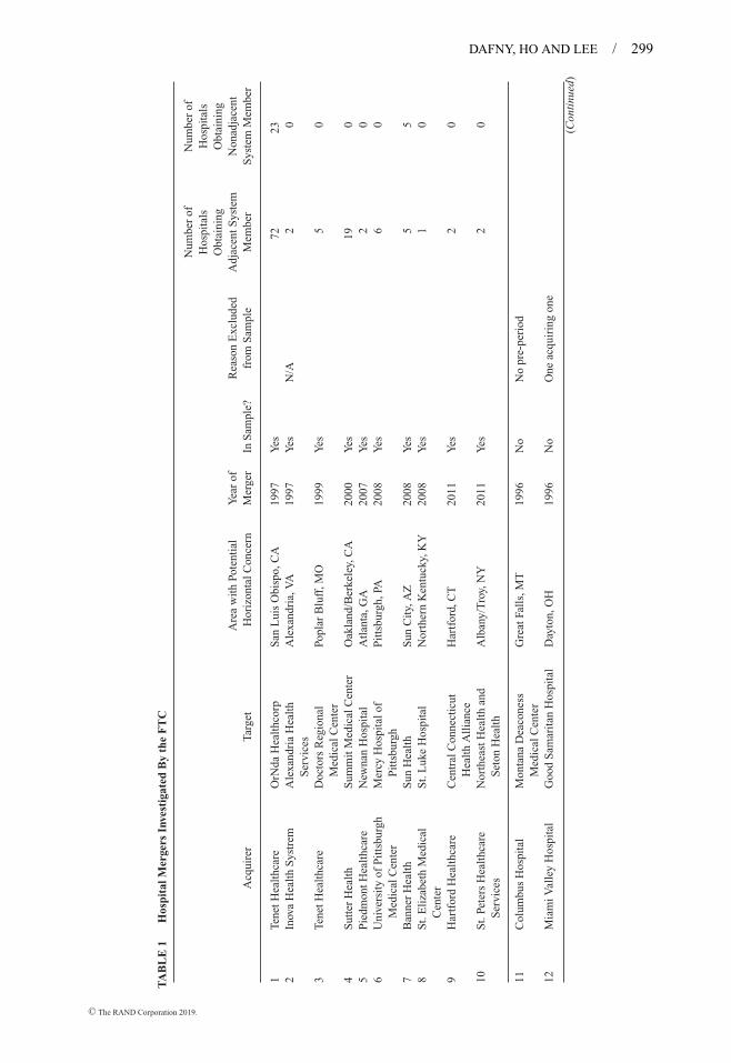
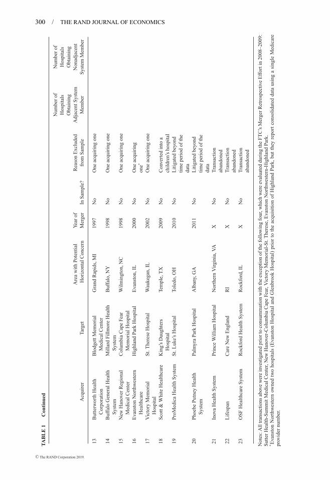
FTC sample. The FTC sample consists of mergers that were investigated by the FTC due to geo-graphic overlap between the merging parties in one or more markets, and eventually consummated(with or without a legal challenge by the FTC).25 Table 1 lists the mergers in the FTC sample andthe geographic market with the closest overlap among the merging parties. Investigations are nottypically announced by competition authorities unless a complaint is issued. However, privateparties may disclose if they are under investigation or are being questioned in connection with anopen investigation.
Combing public sources, we identified 23 investigations of proposed mergers among generalacute-care hospitals over the period 1996–2011.26 Of these 23 mergers, 3 were abandoned bythe would-be merging parties, and 20 were consummated. Given the high costs associated withresponding to an FTC investigation, we posit that these mergers were motivated by the combinationof hospitals in an overlapping geographic market. Otherwise, the merging systems would likelyhave divested a potentially problematic property or abandoned the transaction in the face ofFTC scrutiny. Hence, we consider the two hospitals closest to one another to be the “drivers” of
24 Dafny and Dranove (2009) show that independent hospitals with poor operating performance and stronger“upcoding potential” are more likely to join for-profit hospital systems, and upon joining, to engage in upcoding thatyields higher net revenues per admission.
25 Of the 20 consummated transactions in Table 1, five were challenged by the FTC (Tenet-Doctors Regional inMissouri, Butterworth-Blodgett in Michigan, ProMedica-St. Luke’s in Ohio, Evanston Northwestern-Highland Park inIllinois, and Phoebe Putney-Palmyra Park in Georgia), and one by the California Attorney General (Sutter-Summit). Inone additional transaction (the Tenet-OrNda merger of 1997), the merging parties agreed to divest a hospital located in theoverlap market (French Hospital and Medical Center in San Luis Obispo, CA). As indicated in Table 1, of the transactionschallenged or subject to a divestiture order, only Tenet-Doctors Regional, Sutter-Summit, and Tenet-OrNda are includedin our estimation sample.
26 In 2013, the FTC issued a report stating there were 20 total hospital merger investigations conducted between fiscalyears 1996–2011, pursuant to the Hart Scott Rodino (HSR) Act. These figures include transactions among nongeneralacute-care hospitals, for example, psychiatric hospitals. However, they exclude investigations of so-called “non-HSRreportable transactions.” Nonprofits are subject to less stringent HSR reporting requirements, so in light of the fact thatmany hospitals are nonprofits, the aggregate totals appear to be well aligned with this report. We did not include mergerstaking place in 2012–2014, due to the absence of a post-period in our data on hospital prices.
C© The RAND Corporation 2019.
DAFNY, HO AND LEE / 299
TA
BL
E1
Hos
pita
lMer
gers
Inve
stig
ated
By
the
FT
C
Acq
uire
rTa
rget
Are
aw
ith
Pote
ntia
lH
oriz
onta
lCon
cern
Yea
rof
Mer
ger
InS
ampl
e?R
easo
nE
xclu
ded
from
Sam
ple
Num
ber
ofH
ospi
tals
Obt
aini
ngA
djac
entS
yste
mM
embe
r
Num
ber
ofH
ospi
tals
Obt
aini
ngN
onad
jace
ntS
yste
mM
embe
r
1Te
netH
ealt
hcar
eO
rNda
Hea
lthc
orp
San
Lui
sO
bisp
o,C
A19
97Y
es72
232
Inov
aH
ealt
hS
ystr
emA
lexa
ndri
aH
ealt
hS
ervi
ces
Ale
xand
ria,
VA
1997
Yes
N/A
20
3Te
netH
ealt
hcar
eD
octo
rsR
egio
nal
Med
ical
Cen
ter
Popl
arB
luff
,MO
1999
Yes
50
4S
utte
rH
ealt
hS
umm
itM
edic
alC
ente
rO
akla
nd/B
erke
ley,
CA
2000
Yes
190
5P
iedm
ontH
ealt
hcar
eN
ewna
nH
ospi
tal
Atl
anta
,GA
2007
Yes
20
6U
nive
rsit
yof
Pit
tsbu
rgh
Med
ical
Cen
ter
Mer
cyH
ospi
talo
fP
itts
burg
hP
itts
burg
h,PA
2008
Yes
60
7B
anne
rH
ealt
hS
unH
ealt
hS
unC
ity,
AZ
2008
Yes
55
8S
t.E
liza
beth
Med
ical
Cen
ter
St.
Luk
eH
ospi
tal
Nor
ther
nK
entu
cky,
KY
2008
Yes
10
9H
artf
ord
Hea
lthc
are
Cen
tral
Con
nect
icut
Hea
lth
All
ianc
eH
artf
ord,
CT
2011
Yes
20
10S
t.Pe
ters
Hea
lthc
are
Ser
vice
sN
orth
east
Hea
lth
and
Set
onH
ealt
hA
lban
y/T
roy,
NY
2011
Yes
20
11C
olum
bus
Hos
pita
lM
onta
naD
eaco
ness
Med
ical
Cen
ter
Gre
atFa
lls,
MT
1996
No
No
pre-
peri
od
12M
iam
iVal
ley
Hos
pita
lG
ood
Sam
arit
anH
ospi
tal
Day
ton,
OH
1996
No
One
acqu
irin
gon
e
(Con
tinu
ed)
C© The RAND Corporation 2019.
300 / THE RAND JOURNAL OF ECONOMICS
TA
BL
E1
Con
tinu
ed
Acq
uire
rTa
rget
Are
aw
ith
Pote
ntia
lH
oriz
onta
lCon
cern
Yea
rof
Mer
ger
InS
ampl
e?R
easo
nE
xclu
ded
from
Sam
ple
Num
ber
ofH
ospi
tals
Obt
aini
ngA
djac
entS
yste
mM
embe
r
Num
ber
ofH
ospi
tals
Obt
aini
ngN
onad
jace
ntS
yste
mM
embe
r
13B
utte
rwor
thH
ealt
hC
orpo
rati
onB
lodg
ettM
emor
ial
Med
ical
Cen
ter
Gra
ndR
apid
s,M
I19
97N
oO
neac
quir
ing
one
14B
uffa
loG
ener
alH
ealt
hS
yste
mM
illa
rdFi
llm
ore
Hea
lth
Sys
tem
Buf
falo
,NY
1998
No
One
acqu
irin
gon
e
15N
ewH
anov
erR
egio
nal
Med
ical
Cen
ter
Col
umbi
aC
ape
Fear
Mem
oria
lHos
pita
lW
ilm
ingt
on,N
C19
98N
oO
neac
quir
ing
one
16E
vans
ton
Nor
thw
este
rnH
ealt
hcar
eH
ighl
and
Park
Hos
pita
lE
vans
ton,
IL20
00N
oO
neac
quir
ing
one*
17V
icto
ryM
emor
ial
Hos
pita
lS
t.T
here
seH
ospi
tal
Wau
kega
n,IL
2002
No
One
acqu
irin
gon
e
18S
cott
&W
hite
Hea
lthc
are
Kin
g’s
Dau
ghte
rsH
ospi
tal
Tem
ple,
TX
2009
No
Con
vert
edin
toa
chil
dren
’sho
spit
al19
Pro
Med
ica
Hea
lth
Sys
tem
St.
Luk
e’s
Hos
pita
lTo
ledo
,OH
2010
No
Lit
igat
edbe
yond
tim
epe
riod
ofth
eda
ta20
Pho
ebe
Put
ney
Hea
lth
Sys
tem
Palm
yra
Park
Hos
pita
lA
lban
y,G
A20
11N
oL
itig
ated
beyo
ndti
me
peri
odof
the
data
21In
ova
Hea
lth
Sys
tem
Pri
nce
Wil
liam
Hos
pita
lN
orth
ern
Vir
gini
a,V
AX
No
Tra
nsac
tion
aban
done
d22
Lif
espa
nC
are
New
Eng
land
RI
XN
oT
rans
acti
onab
ando
ned
23O
SF
Hea
lthc
are
Sys
tem
Roc
kfor
dH
ealt
hS
yste
mR
ockf
ord,
ILX
No
Tra
nsac
tion
aban
done
d
Not
es:A
lltr
ansa
ctio
nsab
ove
wer
ein
vest
igat
edpr
ior
toco
nsum
mat
ion
wit
hth
eex
cept
ion
ofth
efo
llow
ing
four
,whi
chw
ere
eval
uate
ddu
ring
the
FT
C’s
Mer
ger
Ret
rosp
ectiv
eE
ffor
tin
2008
–200
9:S
utte
rH
ealt
h-S
umm
itM
edic
alC
ente
r,N
ewH
anov
er-C
olum
bia
Cap
eFe
ar,V
icto
ryM
emor
ial-
St.
The
rese
,Eva
nsto
nN
orth
wes
tern
-Hig
hlan
dPa
rk.
*E
vans
ton
Nor
thw
este
rnow
ned
two
hosp
ital
s(E
vans
ton
Hos
pita
lan
dG
lenb
rook
Hos
pita
l)pr
ior
toth
eac
quis
itio
nof
Hig
hlan
dPa
rk,
but
they
repo
rtco
nsol
idat
edda
taus
ing
asi
ngle
Med
icar
epr
ovid
ernu
mbe
r.
C© The RAND Corporation 2019.
DAFNY, HO AND LEE / 301
FIGURE 1
DEFINING TREATMENT GROUPS, FTC SAMPLE[Color figure can be viewed at wileyonlinelibrary.com]
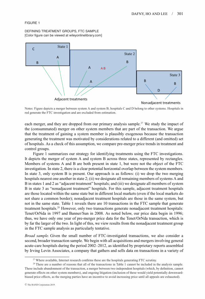
Notes: Figure depicts a merger between system A and system B; hospitals C and D belong to other systems. Hospitals inred generate the FTC investigation and are excluded from estimation.
each merger, and they are dropped from our primary analysis sample.27 We study the impact ofthe (consummated) merger on other system members that are part of the transaction. We arguethat the treatment of gaining a system member is plausibly exogenous because the transactiongenerating the treatment was motivated by considerations related to a different (and omitted) setof hospitals. As a check of this assumption, we compare pre-merger price trends in treatment andcontrol groups.
Figure 1 summarizes our strategy for identifying treatments using the FTC investigations.It depicts the merger of system A and system B across three states, represented by rectangles.Members of systems A and B are both present in state 1, but were not the object of the FTCinvestigation. In state 2, there is a clear potential horizontal overlap between the system members.In state 3, only system B is present. Our approach is as follows: (i) we drop the two merginghospitals nearest one another in state 2; (ii) we designate all remaining members of systems A andB in states 1 and 2 as “adjacent treatment” hospitals; and (iii) we designate all members of systemB in state 3 as “nonadjacent treatment” hospitals. For this sample, adjacent treatment hospitalsare those located within the same state but in different local markets (even if the local markets donot share a common border); nonadjacent treatment hospitals are those in the same system, butnot in the same state. Table 1 reveals there are 10 transactions in the FTC sample that generatetreatment hospitals.28 However, only two transactions generate nonadjacent treatment hospitals:Tenet/OrNda in 1997 and Banner/Sun in 2008. As noted below, our price data begin in 1996;thus, we have only one year of pre-merger price data for the Tenet/OrNda transaction, which isby far the larger of the two. In light of this, we view results from the nonadjacent treatment groupin the FTC sample analysis as particularly tentative.
Broad sample. Given the small number of FTC-investigated transactions, we also consider asecond, broader transaction sample. We begin with all acquisitions and mergers involving generalacute-care hospitals during the period 2002–2012, as identified by proprietary reports assembledby Irving Levin Associates, a company that gathers and sells data on transactions in a variety of
27 Where available, Internet research confirms these are the hospitals generating FTC scrutiny.28 There are a number of reasons that all of the transactions in Table 1 cannot be included in the analysis sample.
These include abandonment of the transaction, a merger between two independent hospitals (which, by definition, cannotgenerate effects on other system members), and ongoing litigation (inclusion of these would yield potentially downward-biased price effects, as the merging parties have an incentive to avoid increasing price until all appeals are exhausted).
C© The RAND Corporation 2019.

302 / THE RAND JOURNAL OF ECONOMICS
FIGURE 2
DEFINING TREATMENT GROUPS, BROAD SAMPLE[Color figure can be viewed at wileyonlinelibrary.com]
Notes: Figure depicts the 2007 merger between Catholic Healthcare Partners (CHP) and Baptist Health System (BHS).The largest BHS hospital (noted “Crown Jewel”) is dropped from the estimation sample, as are all hospitals from opposingsystems located within 30 minutes’ drive of one another.
sectors, including the US hospital industry. As our strategy relies on examining the impact of amerger on bystander hospitals, we exclude mergers between independent hospitals. We imposetwo additional restrictions. First, we drop the “crown jewels” of each transaction, defined as thelargest hospital being acquired for transactions involving five or fewer hospitals, and all hospitalsabove the 80th percentile of beds among target systems with more than five hospitals. Second, wedrop hospitals gaining a system member within 30 minutes’ drive, as there may be “same-market”motivations and effects in these cases.
Our effort to focus on bystanders to a transaction is designed to minimize omitted variablesbias. To the extent that transactions are motivated by crown jewels and/or within-market overlaps,then the impact of the transactions on other system members is plausibly exogenous to omitteddeterminants of price. Whereas the transactions may be motivated in part (or in whole) byanticipation of price increases due to cross-market effects, our identifying assumptions requirethat they are not made in anticipation of unobserved cost or demand shocks that may themselvesgenerate systematic price increases. As the largest assets in a transaction, the crown jewels of atarget system seem likeliest to be acquired because of such unobserved (to the econometrician)shocks, hence we omit them (as well as the within-market overlaps).
In both samples, we investigate the potential for bias due to omitted factors by includingleads for the transactions in our specifications; the coefficients on these leads will reveal whethertreatment hospitals have pre-treatment price trends similar to those of control hospitals. Althoughthis test cannot rule out the possibility that price trends for bystanders and controls may subse-quently diverge for unobserved reasons coincident with but independent of the merger, it stillinforms the plausibility of our identifying assumptions.
Figure 2 summarizes our strategy for identifying treatments using the broad merger sample,using as an example the 2007 acquisition of 4-hospital Baptist Health System (BHS) in Tennesseeby Catholic Healthcare Partners (CHP), with 30 hospitals in and outside of Tennessee. The largestBHS hospital is dropped as the presumed acquisition target (crown jewel), and two BHS and oneCHP hospitals are dropped for being within 30 minutes of each other. This leaves one BHSand three CHP hospitals in Tennessee as potential treatment hospitals. In our main analysis, weadopt the same convention as in the FTC sample and use state boundaries to determine whetherhospitals are considered to be within the adjacent or nonadjacent treatment groups. Thus, the
C© The RAND Corporation 2019.

DAFNY, HO AND LEE / 303
TABLE 2 Hospital Merger Transaction Statistics in Broad Sample, 2002–2012
Acquirer Size(number of hospitals)
Target Size(number of hospitals)
Transaction FilterNumber of
Transactions Median Mean Median Mean
All transactions (from Irving Levin*) 426 9.0 24.0 1.0 1.6Generates 1+ treatment hospitals 332 17.0 30.2 1.0 1.7Generates 1+ adjacent treatment
hospitals270 23.0 33.8 1.0 1.8
Generates 1+ nonadjacent treatmenthospitals
240 29.0 39.4 1.0 2.0
Clean in the two years before andafter treatment and:
Generates 1+ treatment hospitals 52 5.0 9.4 1.0 1.3Generates 1+ adjacent treatment
hospitals43 5.0 8.8 1.0 1.3
Generates 1+ nonadjacent treatmenthospitals
22 8.5 15.9 1.0 1.6
Notes: “Clean in the two years before and after treatment” means that the hospital is unaffected (either directly or bybeing within 30 minutes’ drive of an affected hospital) by other mergers during this period. We consider only transactionsinvolving “consolidation,” which is defined as an existing hospital or system gaining members (as opposed to, say, atransfer of assets). This definition captures 85% of the deals in the Irving Levin Hospital Acquisition Reports.
four remaining hospitals in Tennessee are part of the the adjacent treatment group, whereas allCHP hospitals outside Tennessee are nonadjacent treatments. Note that this example illustratesall of our restrictions on a single transaction, however, it is rare for target hospitals to survivethe sample restrictions (as one did in this case). In Section 5, we consider alternative definitionsfor “adjacency,” including a measure based on the shortest distance between merging hospitals(rather than state boundaries).
Table 2 presents descriptive information for the set of mergers in our broad sample thatoccurred between 2002 and 2012. In all, there are 426 transactions, 332 of which generateadjacent and/or nonadjacent treatment hospitals. This larger sample size enables us to take moresteps to ensure a clean treated sample than is possible when analyzing the FTC sample. We limitour treatment sample to hospitals experiencing a treatment only once during the five-year periodspanning the transaction generating that treatment, that is, all treatment hospitals must be exposedto no other mergers from t = −2 to t = 2.29 Relative to the set of all transactions, transactions thatare included in our final analysis sample involve smaller acquirers (as measured by the number offacilities), as larger acquirers tend to engage in multiple closely timed acquisitions. Unchangedis the median size of targets, which is a single hospital.
� Data and descriptive statistics. We construct a measure of each hospital’s commercialprice for a standardized inpatient admission using the Healthcare Cost Report Information System(HCRIS) data set for fiscal years 1996–2012, following the methodology in Dafny (2009). Thismeasure is constructed by dividing an estimate of net inpatient revenue for non-Medicare patientsby the total number of non-Medicare inpatient admissions. We deviate from Dafny (2009) slightly
29 Data for treatment hospitals that are “clean” for longer periods of time are included between t = −3 up to t= 4, so as to expand our observation period. We use supplemental Irving Levin data from 2000 and 2001, and manualchecks for 2013–2014, to ensure that any “treated” hospitals are “clean” (i.e., untreated) for the two years before and afterany merger included in our sample. Requiring a longer “clean” period for all treatment hospitals—that is, for the entireeight year period in our regressions (t = −3 to t = 4)—would exclude too many mergers from our sample. Of the 52transactions with a clean treatment hospital from t = −2 to t = 2, 35 have a clean treatment hospital from t = −3 to t =3, and 27 have a clean treatment hospital from t = −3 to t = 4. We could not impose this restriction in the FTC samplebecause the largest of the two transactions generating treatments occurred in 1997 and we lack merger data in prior years.
C© The RAND Corporation 2019.
304 / THE RAND JOURNAL OF ECONOMICS
TABLE 3 Descriptive Statistics
Panel A: FTC Sample
Adjacent Treatments Nonadjacent Treatments Control Group 1 Control Group 2
Number of hospitals 116 28 4706 2692acquiring/target 88/28 21/7 N/A N/A
CMI 1.43 1.36 1.28 1.35Beds 207 157 151 181% Medicaid 15.8% 16.9% 14.0% 13.6%For-profit 64.2% 80.4% 17.3% 25.3%Urban 88.8% 71.4% 58.4% 69.2%Census RegionMidwest 6.0% 0.0% 30.5% 28.8%Northeast 8.6% 3.6% 13.8% 13.0%South 37.1% 57.1% 38.7% 42.4%West 48.3% 39.3% 17.0% 15.8%
Panel B: Broad Sample
Number of hospitals 104 55 4755 756number of hospitals (full data) 81 38 4055 592
acquiring/target 76/5 37/1 N/A N/ACMI 1.31 1.26 1.29 1.32Beds 147 148 153 174% Medicaid 12.5% 12.5% 14.4% 13.1%For-profit 6.1% 6.6% 21.7% 6.3%Urban 49.4% 44.7% 60.3% 65.2%Census RegionMidwest 42.0% 63.2% 26.9% 32.3%Northeast 4.9% 2.6% 15.0% 23.1%South 40.7% 21.1% 39.0% 31.6%West 12.3% 13.2% 19.1% 13.0%
Notes: The unit of observation is the hospital-year unless otherwise noted.
by including the hospital’s Medicare case-mix index as a control for patient complexity in allspecifications, rather than incorporating it directly in the denominator of price. For additionaldetails and a discussion of how this price measure compares to price data from other sources, seeAppendix B.1.
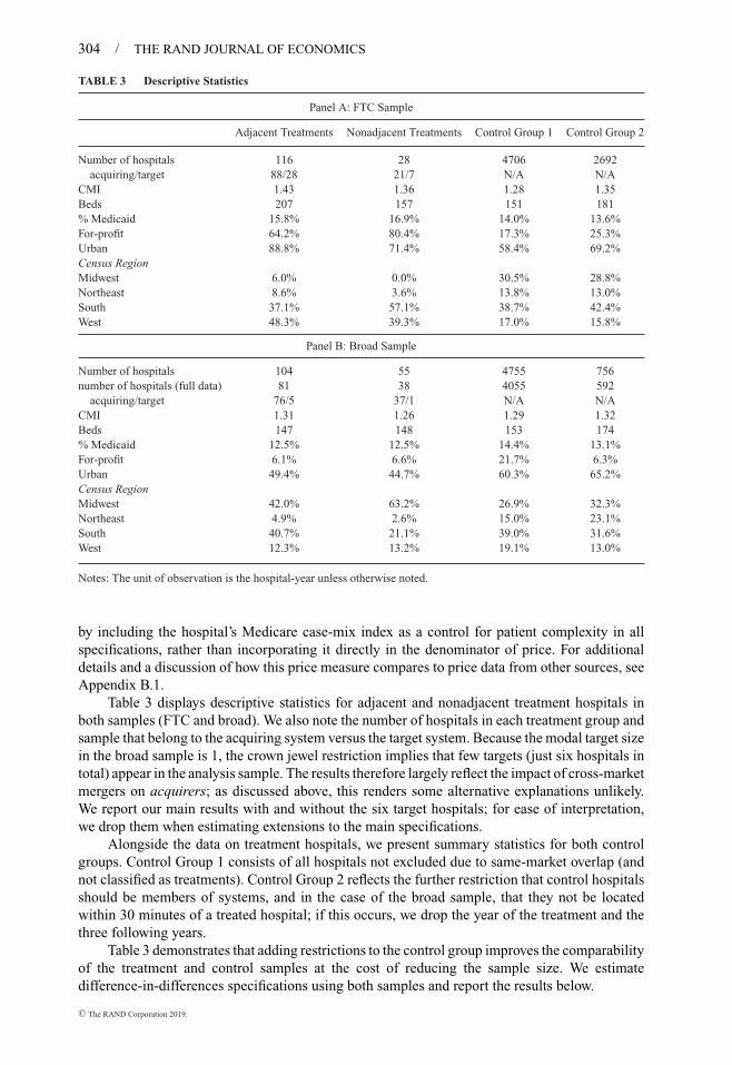
Table 3 displays descriptive statistics for adjacent and nonadjacent treatment hospitals inboth samples (FTC and broad). We also note the number of hospitals in each treatment group andsample that belong to the acquiring system versus the target system. Because the modal target sizein the broad sample is 1, the crown jewel restriction implies that few targets (just six hospitals intotal) appear in the analysis sample. The results therefore largely reflect the impact of cross-marketmergers on acquirers; as discussed above, this renders some alternative explanations unlikely.We report our main results with and without the six target hospitals; for ease of interpretation,we drop them when estimating extensions to the main specifications.
Alongside the data on treatment hospitals, we present summary statistics for both controlgroups. Control Group 1 consists of all hospitals not excluded due to same-market overlap (andnot classified as treatments). Control Group 2 reflects the further restriction that control hospitalsshould be members of systems, and in the case of the broad sample, that they not be locatedwithin 30 minutes of a treated hospital; if this occurs, we drop the year of the treatment and thethree following years.
Table 3 demonstrates that adding restrictions to the control group improves the comparabilityof the treatment and control samples at the cost of reducing the sample size. We estimatedifference-in-differences specifications using both samples and report the results below.
C© The RAND Corporation 2019.

DAFNY, HO AND LEE / 305
4. Empirical results: how do cross-market mergers affect hospitalprices?
� We quantify the impact on price of becoming an adjacent or nonadjacent party to a merger,relative to a sample of control hospitals over the same relevant time period. We estimate fixed-effects models of the following form:
ln(priceht ) = αh +∑
l
φal 1adj
h,t=m(h)+l +∑
g
φng 1nadj
h,t=m(h)+g + Xhtθ + τt + εht . (9)
where h indexes hospitals, t indexes years, and m(h) denotes the year of the relevant transaction forhospital h; 1adj
h,· and 1nadjh,· are indicators for whether hospital h belongs to the adjacent or nonadjacent
treatment group in the relevant year; and Xht are hospital characteristics including ln(case-mixindex), ln(beds), a for-profit ownership dummy, and percent of admissions to Medicaid enrollees.Given the inclusion of hospital and year fixed effects, coefficients on these variables are identifiedby within-hospital changes in these factors.
In our first specification, we include the maximum number of leads and lags permittedin each sample: for the reasons discussed in Section 3, l = −2 . . . 4 for both the FTC and thebroad merger analysis, and g = 0 . . . 4 for the FTC analysis and −2 . . . 4 for the broad mergeranalysis. The purpose of this model is twofold: first, to confirm the leads lack a pronouncedtrend (to support the contention that the price trajectory of the control hospitals is a reasonablecounterfactual for the treatment hospitals absent the treatment); second, to examine how the priceeffect (if any) changes over time.
We also estimate a second specification where the treatment leads and lags are replaced withtwo variables for each treatment, an indicator variable for the year of the merger and anotherwhich takes a value of 1 in every subsequent year:
ln(priceht ) = αh + φat=m(h)1
adjh,t=m(h) + φa
t>m(h)1adjh,t>m(h) + φn
t=m(h)1nadjh,t=m(h) (10)
+ φnt>m(h)1
nadjh,t>m(h) + Xhtθ + τt + εht .
Combining the post-merger years into a single dummy increases the precision of our estimatesand provides a single-point estimate for the price effect of each treatment. The specificationallows for a different price effect in year t = 0, as mergers may close at any point during the yearin which they are recorded and hence t = 0 does not strictly fall into the pre- or post-periods.In all regressions, observations are weighted by the hospital’s number of discharges (averagedacross all years), and standard errors are clustered by hospital.30
These models assume that treatment status is exogenous to omitted determinants of price.As previously described, our sample excludes hospitals that are the likely drivers of transactions.The rationale is that “bystanders” to transactions are unlikely to differ in unobservable ways fromnonbystanders, that is, control hospitals. Threats to identification are unobservable factors thatdifferentially influence the negotiated prices for hospitals involved in mergers during the post-merger period versus hospitals in our control groups. For example, in the broad merger sample,hospitals that are never treated may have internally focused managers who are not entrepreneurialabout seeking new partners and potentially less likely to negotiate steady price increases withpayers (as most hospitals did throughout this time period). Alternatively, some merger targetsmay be chosen (based on unobservables) specifically to generate the cross-market price effectswe seek to study. These unobservables will not bias our estimates unless they have a differentialeffect on price during the pre- and post-acquisition period. To explore this concern, we alsoestimate models in which we pair each treatment hospital with its closest match in the controlgroup, as identified using a propensity score model. We then estimate a “differenced regression”
30 Although all tables report standard errors with clustering at the hospital unit, the results are robust to clusteringby transaction or by state.
C© The RAND Corporation 2019.

306 / THE RAND JOURNAL OF ECONOMICS
FIGURE 3
FTC LEADS AND LAGS (CONTROL GROUP 2) [Color figure can be viewed at wileyonlinelibrary.com]
that focuses on changes in price for each treatment relative to its closest match. As we discussbelow, the results are broadly similar.
We now describe the results for each of the transaction samples in turn.
� FTC sample. The results from estimating equation (9) using the FTC-investigated mergersample are presented in Appendix Table B1. As discussed above, we report findings obtainedusing two control groups. Control Group 1 is very broad; Control Group 2 is restricted to hospitalsthat are system members and hence more similar to the treatment groups (which must be systemmembers). The results are similar across the two samples. Figure 3 graphs the coefficient estimateson the leads and lags of the adjacent and nonadjacent indicator variable from equation (9) above,as estimated using Control Group 2. Beginning with the price patterns for adjacent hospitals, wesee that price jumps up for these hospitals in t = −2 (relative to the omitted year, t = −3) byabout 7 %, and then holds steady until t = 0. Prices increase steadily from t = 1 to t = 4, at whichpoint the price of adjacent treatment hospitals is 17%–18% higher than that of the control group,all else equal. nonadjacent hospitals, for which we only have one year of pre-merger data, exhibita statistically insignificant reduction in price in the year of the merger, after which prices fluctuateand ultimately end up slightly lower—albeit not significantly so—than where they started. We canreject equality of the coefficients on the adjacent and nonadjacent indicators in t = 4 at p < 0.05.
Most of the control variables have statistically significant coefficients. In both samples,increases in the complexity of a hospital’s caseload, and in its number of staffed beds, areassociated with higher prices. The for-profit dummy is also positive and statistically significantin both models. Given the inclusion of hospital fixed effects, the interpretation is that hospitalsthat convert to for-profit status experience price increases, all else equal. Changes in Medicaidpatient share are not associated with significant changes in private price.31
Table 4 presents coefficient estimates from the parsimonious regression equation (10),in which we include indicators for t = 0 and t > 0 (separately for adjacent and nonadjacenttreatment groups). The results show that the adjacent treatment leads to a statistically significantprice increase of roughly 7%, whereas nonadjacent treatment is not linked to any significant
31 As noted below, Appendix Table B4 reports results dropping all control variables, and they are very similar tothe results including the controls.
C© The RAND Corporation 2019.
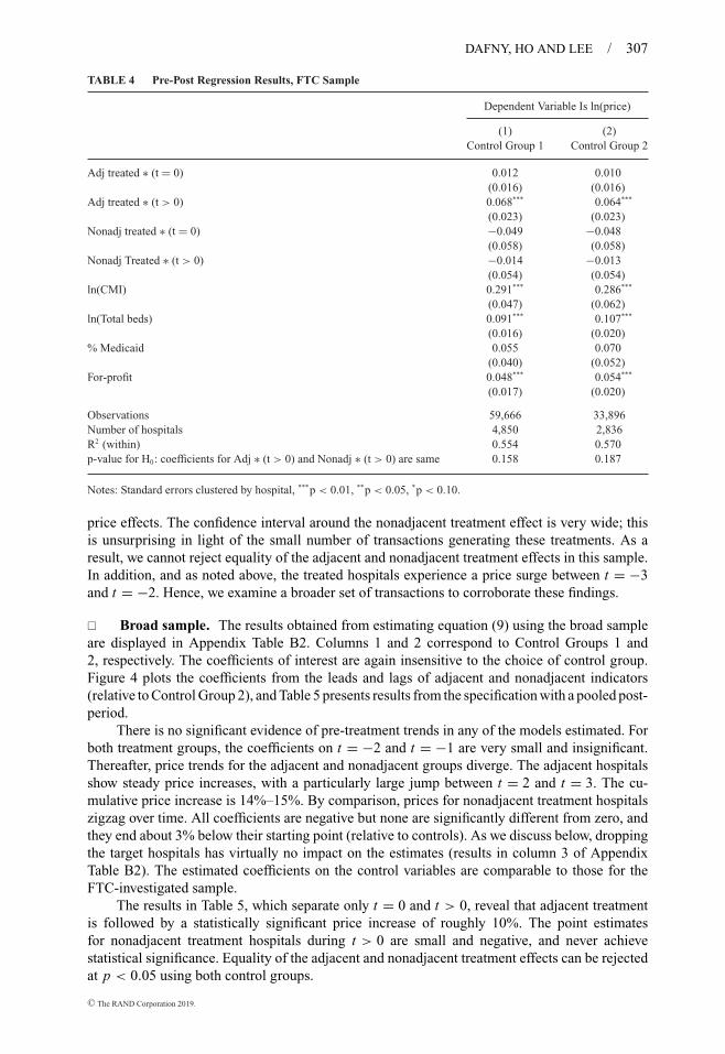
DAFNY, HO AND LEE / 307
TABLE 4 Pre-Post Regression Results, FTC Sample
Dependent Variable Is ln(price)
(1) (2)Control Group 1 Control Group 2
Adj treated ∗ (t = 0) 0.012 0.010(0.016) (0.016)
Adj treated ∗ (t > 0) 0.068*** 0.064***
(0.023) (0.023)Nonadj treated ∗ (t = 0) −0.049 −0.048
(0.058) (0.058)Nonadj Treated ∗ (t > 0) −0.014 −0.013
(0.054) (0.054)ln(CMI) 0.291*** 0.286***
(0.047) (0.062)ln(Total beds) 0.091*** 0.107***
(0.016) (0.020)% Medicaid 0.055 0.070
(0.040) (0.052)For-profit 0.048*** 0.054***
(0.017) (0.020)
Observations 59,666 33,896Number of hospitals 4,850 2,836R2 (within) 0.554 0.570p-value for H0: coefficients for Adj ∗ (t > 0) and Nonadj ∗ (t > 0) are same 0.158 0.187
Notes: Standard errors clustered by hospital, ***p < 0.01, **p < 0.05, *p < 0.10.
price effects. The confidence interval around the nonadjacent treatment effect is very wide; thisis unsurprising in light of the small number of transactions generating these treatments. As aresult, we cannot reject equality of the adjacent and nonadjacent treatment effects in this sample.In addition, and as noted above, the treated hospitals experience a price surge between t = −3and t = −2. Hence, we examine a broader set of transactions to corroborate these findings.
� Broad sample. The results obtained from estimating equation (9) using the broad sampleare displayed in Appendix Table B2. Columns 1 and 2 correspond to Control Groups 1 and2, respectively. The coefficients of interest are again insensitive to the choice of control group.Figure 4 plots the coefficients from the leads and lags of adjacent and nonadjacent indicators(relative to Control Group 2), and Table 5 presents results from the specification with a pooled post-period.
There is no significant evidence of pre-treatment trends in any of the models estimated. Forboth treatment groups, the coefficients on t = −2 and t = −1 are very small and insignificant.Thereafter, price trends for the adjacent and nonadjacent groups diverge. The adjacent hospitalsshow steady price increases, with a particularly large jump between t = 2 and t = 3. The cu-mulative price increase is 14%–15%. By comparison, prices for nonadjacent treatment hospitalszigzag over time. All coefficients are negative but none are significantly different from zero, andthey end about 3% below their starting point (relative to controls). As we discuss below, droppingthe target hospitals has virtually no impact on the estimates (results in column 3 of AppendixTable B2). The estimated coefficients on the control variables are comparable to those for theFTC-investigated sample.
The results in Table 5, which separate only t = 0 and t > 0, reveal that adjacent treatmentis followed by a statistically significant price increase of roughly 10%. The point estimatesfor nonadjacent treatment hospitals during t > 0 are small and negative, and never achievestatistical significance. Equality of the adjacent and nonadjacent treatment effects can be rejectedat p < 0.05 using both control groups.
C© The RAND Corporation 2019.

308 / THE RAND JOURNAL OF ECONOMICS
FIGURE 4
BROAD SAMPLE LEADS AND LAGS (CONTROL GROUP 2) [Color figure can be viewed atwileyonlinelibrary.com]
� Robustness of main results. We investigate the robustness of our results to alternativespecifications. One possible concern regarding the FTC sample, given the small number oftransactions in the data, is that the estimated price effects could be driven by a single merger. Werepeat the main analysis excluding one merger at a time. The results are presented in AppendixTable B3. The estimates are very stable across these samples.
We also test the robustness of the results to inclusion of a for-profit indicator interactedwith individual year dummies. Per Table 3 (Descriptive Statistics), treated hospitals in the FTCsample are far likelier to be for-profit than hospitals in either control group (in the broadsample, for-profit ownership is similar across the treatment group and Control Group 2). Iffor-profit hospitals have different price trajectories, then our estimated treatment effects couldbe reflecting this difference. However, the results (in Appendix Table B4, reported for bothsamples using Control Group 2) are exceedingly similar, even allowing for different year ef-fects for for-profit hospitals. We also estimate models excluding all control variables. Thecoefficients of interest, in columns 2 and 5 of Appendix Table B4, are virtually unchanged;this finding alleviates the concern that omitted, time-varying hospital and market character-istics that are correlated with price (as the controls are) are also correlated with treatmentstatus.
Last, we develop a model that involves matching treatment hospitals to specific controlhospitals. We estimate regressions analogous to those described above, but replacing the vari-ables with the differences between each treatment and its matched control(s). One advantageof this approach is that it admits heterogeneous time trends for different pairs of hospitals andmatched controls.
The regression is below:
ln(priceht/pricec(h),t ) = αh +∑
l
φal 1adj
h,t=m(h)+l +∑
g
φng 1nadj
h,t=m(h)+g
+ (Xht − Xc(h)t )θ + εht . (11)
C© The RAND Corporation 2019.
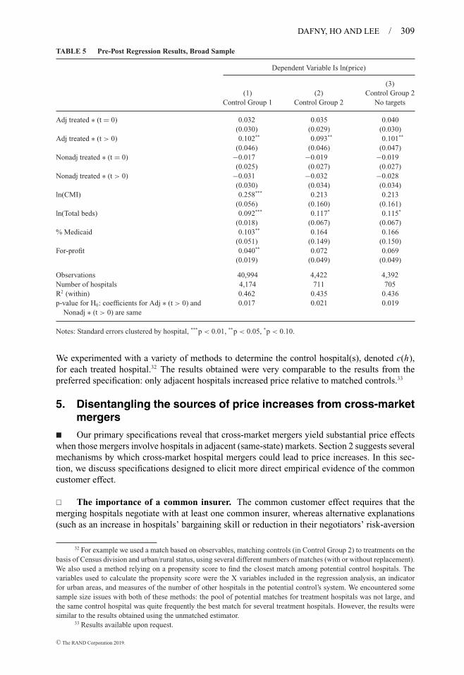
DAFNY, HO AND LEE / 309
TABLE 5 Pre-Post Regression Results, Broad Sample
Dependent Variable Is ln(price)
(3)(1) (2) Control Group 2
Control Group 1 Control Group 2 No targets
Adj treated ∗ (t = 0) 0.032 0.035 0.040(0.030) (0.029) (0.030)
Adj treated ∗ (t > 0) 0.102** 0.093** 0.101**
(0.046) (0.046) (0.047)Nonadj treated ∗ (t = 0) −0.017 −0.019 −0.019
(0.025) (0.027) (0.027)Nonadj treated ∗ (t > 0) −0.031 −0.032 −0.028
(0.030) (0.034) (0.034)ln(CMI) 0.258*** 0.213 0.213
(0.056) (0.160) (0.161)ln(Total beds) 0.092*** 0.117* 0.115*
(0.018) (0.067) (0.067)% Medicaid 0.103** 0.164 0.166
(0.051) (0.149) (0.150)For-profit 0.040** 0.072 0.069
(0.019) (0.049) (0.049)
Observations 40,994 4,422 4,392Number of hospitals 4,174 711 705R2 (within) 0.462 0.435 0.436p-value for H0: coefficients for Adj ∗ (t > 0) and
Nonadj ∗ (t > 0) are same0.017 0.021 0.019
Notes: Standard errors clustered by hospital, ***p < 0.01, **p < 0.05, *p < 0.10.
We experimented with a variety of methods to determine the control hospital(s), denoted c(h),for each treated hospital.32 The results obtained were very comparable to the results from thepreferred specification: only adjacent hospitals increased price relative to matched controls.33
5. Disentangling the sources of price increases from cross-marketmergers
� Our primary specifications reveal that cross-market mergers yield substantial price effectswhen those mergers involve hospitals in adjacent (same-state) markets. Section 2 suggests severalmechanisms by which cross-market hospital mergers could lead to price increases. In this sec-tion, we discuss specifications designed to elicit more direct empirical evidence of the commoncustomer effect.
� The importance of a common insurer. The common customer effect requires that themerging hospitals negotiate with at least one common insurer, whereas alternative explanations(such as an increase in hospitals’ bargaining skill or reduction in their negotiators’ risk-aversion
32 For example we used a match based on observables, matching controls (in Control Group 2) to treatments on thebasis of Census division and urban/rural status, using several different numbers of matches (with or without replacement).We also used a method relying on a propensity score to find the closest match among potential control hospitals. Thevariables used to calculate the propensity score were the X variables included in the regression analysis, an indicatorfor urban areas, and measures of the number of other hospitals in the potential control’s system. We encountered somesample size issues with both of these methods: the pool of potential matches for treatment hospitals was not large, andthe same control hospital was quite frequently the best match for several treatment hospitals. However, the results weresimilar to the results obtained using the unmatched estimator.
33 Results available upon request.
C© The RAND Corporation 2019.
310 / THE RAND JOURNAL OF ECONOMICS
post-merger; cf. Lewis and Pflum, 2015) do not. We therefore investigate the importance ofcommon insurers in generating a price effect. We create a measure of insurer overlap usingCBSA-level market shares for comprehensive medical insurance, constructed from 2012 datafrom the National Association of Insurance Commissioners. We define insurers at the state level,for example, Cigna in Texas is not pooled with Cigna in Oregon. Although insurers and healthcareproviders do sometimes negotiate at regional and even national levels, within-state overlap ofinsurers is likely to be most relevant for the cross-market mechanisms we model.
The measure we define—insurer overlap—is hospital- and transaction-specific, and contin-uous and monotonic in the degree of joint significance of the same insurers to a given treatmenthospital and to the target system.34 To construct the overlap measure, we proceed in three steps.First, we compute the average market share of every insurer for each target system by taking thebed-weighted average, across each of the system’s hospitals, of each insurer’s market share in thathospital’s CBSA (or non-CBSA portions of the relevant state, if not located in a CBSA). Next,for each treatment hospital in our sample (which now consists solely of members of acquiringsystems), we compare the vector of insurer market shares in that treatment hospital’s CBSA (ornon-CBSA portions of the state) with the vector of insurer average market shares for the targetsystem. Our insurer overlap measure for a treatment hospital and transaction is the sum of thecomponent-wise minimum across these two vectors.
The insurer overlap measure is bounded by 0 and 1, equaling 0 if the treatment hospitaland target system share no insurers, and 1 if they are located in the same CBSA. By definition,nonadjacent treatment hospitals (who gain a system member outside the state) are assigned avalue of 0 for insurer overlap. The interquartile range is [0.51,0.96], with a median of 0.82. Weestimate a specification that incorporates an interaction between the adjacent treatment effect andinsurer overlap. (Because insurer overlap varies at the hospital level, we do not include it directlyin the model, as it is collinear with the hospital fixed effects.) The coefficient on the interactionterm adjacent treated ∗ (t > 0) ∗ insurer overlap is positive but noisily estimated (point estimate0.025, standard error 0.029). Importantly, it absorbs all of the merger price effect (i.e., the pointestimate for the coefficient on the noninteracted term adjacent treated ∗ (t > 0)—around 0.10without the interaction—is now negative and very imprecisely estimated with a point estimateof −0.09 and standard error 0.25). This constitutes suggestive evidence that insurer overlap iscritical to generating post-merger price increases for adjacent treatment hospitals; unfortunately,we lack more precise data that would be ideal for testing our hypothesis (i.e., insurer marketshares for each hospital and year).
� The role of common customers. We next investigate the impact of sharing commoncustomers on merger price effects. We first attempt to construct hospital-specific measures ofcommon customers for all treatment hospitals. An ideal measure of common customers wouldcapture two factors: (i) the relative significance of employers who draw employees from bothtarget and acquirer hospitals; (ii) the volume of employees who commute between both target andacquirer service areas. A proxy for factor (i) could be constructed using information on multisiteestablishments and identifying which sites are in each hospital’s primary service area. Regrettably,this information can only be acquired through on-site access to Census data, coupled with accessto national hospital discharge data to construct hospitals’ primary service areas. A second optionis to use public data on commuting patterns between counties to capture factor (ii). The Censuspublishes such data using the American Community Survey as the primary source.35 We consid-ered two hospital- and transaction-specific measures: an outflow-only measure (defined as the totalshare of county residents commuting to counties in which a hospital acquires a new system mem-ber), and an outflow and inflow measure constructed as the sum of residents commuting between
34 For ease of interpretation, we drop the six treatment hospitals that are members of a target system. The results ofdoing so (for the pooled post-period model) are reported in column 3 of Table 5: there is very little change in the estimates.
35 The data are available at www.census.gov/population/metro/data/other.html. We use information on the numberof commuters from county of residence to county of workplace, by county pair, averaged over the period 2006–2010.
C© The RAND Corporation 2019.
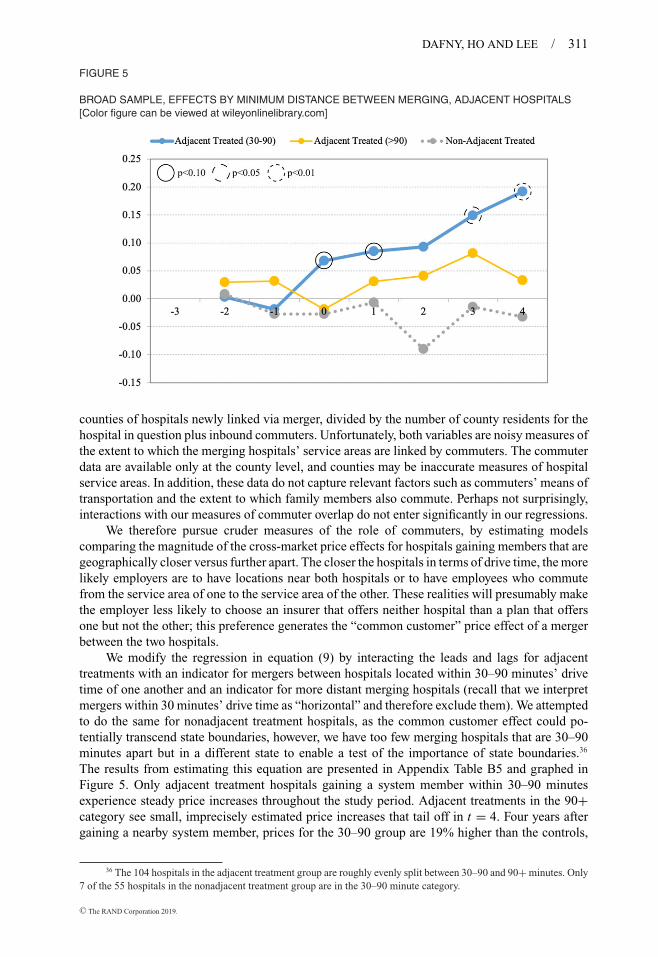
DAFNY, HO AND LEE / 311
FIGURE 5
BROAD SAMPLE, EFFECTS BY MINIMUM DISTANCE BETWEEN MERGING, ADJACENT HOSPITALS[Color figure can be viewed at wileyonlinelibrary.com]
counties of hospitals newly linked via merger, divided by the number of county residents for thehospital in question plus inbound commuters. Unfortunately, both variables are noisy measures ofthe extent to which the merging hospitals’ service areas are linked by commuters. The commuterdata are available only at the county level, and counties may be inaccurate measures of hospitalservice areas. In addition, these data do not capture relevant factors such as commuters’ means oftransportation and the extent to which family members also commute. Perhaps not surprisingly,interactions with our measures of commuter overlap do not enter significantly in our regressions.
We therefore pursue cruder measures of the role of commuters, by estimating modelscomparing the magnitude of the cross-market price effects for hospitals gaining members that aregeographically closer versus further apart. The closer the hospitals in terms of drive time, the morelikely employers are to have locations near both hospitals or to have employees who commutefrom the service area of one to the service area of the other. These realities will presumably makethe employer less likely to choose an insurer that offers neither hospital than a plan that offersone but not the other; this preference generates the “common customer” price effect of a mergerbetween the two hospitals.
We modify the regression in equation (9) by interacting the leads and lags for adjacenttreatments with an indicator for mergers between hospitals located within 30–90 minutes’ drivetime of one another and an indicator for more distant merging hospitals (recall that we interpretmergers within 30 minutes’ drive time as “horizontal” and therefore exclude them). We attemptedto do the same for nonadjacent treatment hospitals, as the common customer effect could po-tentially transcend state boundaries, however, we have too few merging hospitals that are 30–90minutes apart but in a different state to enable a test of the importance of state boundaries.36
The results from estimating this equation are presented in Appendix Table B5 and graphed inFigure 5. Only adjacent treatment hospitals gaining a system member within 30–90 minutesexperience steady price increases throughout the study period. Adjacent treatments in the 90+category see small, imprecisely estimated price increases that tail off in t = 4. Four years aftergaining a nearby system member, prices for the 30–90 group are 19% higher than the controls,
36 The 104 hospitals in the adjacent treatment group are roughly evenly split between 30–90 and 90+ minutes. Only7 of the 55 hospitals in the nonadjacent treatment group are in the 30–90 minute category.
C© The RAND Corporation 2019.

312 / THE RAND JOURNAL OF ECONOMICS
compared to a (statistically insignificant) 3% higher and 3% lower for the 90+ adjacent treatmentsand nonadjacent treatments, respectively. Pooling across the entire post-merger period, we canreject equality of the 30–90 coefficient and the nonadjacent treatment coefficient. We interpretthese findings as consistent with the existence of common customer effects.
� The impact of acquirer and target size. In the seventh subsection of Section 2, we outlinethe theoretical predictions regarding acquirer and target size. To test these hypotheses, we addinteractions between the adjacent ∗ (t > 0) term (the “post-treatment dummy”) and two separateindicators, one for “above median” acquirer size and the second for “above median” target size,where size is measured as market share of all beds in the (same-state) CBSAs, where either or bothacquirer and target operate. We also include a triple interaction between the post-treatment dummyand both size indicators; the coefficient on this interaction will isolate the difference in price effectsfor hospitals where both merging parties are relatively large. For ease of interpretation, we excludeall target hospitals from the estimation sample. Collectively, these variables isolate the effects ofmergers on the four combinations of acquirer size indicator and target size indicator. The resultsare reported in Table 6. Beneath the coefficient estimates, we present linear combinations of therelevant coefficients (and associated standard errors). Price increases are statistically significantfor three of the four groups. Consistent with the predictions of our model (laid out in the seventhsubsection of Section 2), we find that small acquirers raise price more following the acquisitionof a large (relative to a small) target. Further, and again consistent with the theory, the price effectof purchasing a small target is increasing in acquirer size. (Note that the median acquirer shareis 0.14, whereas the median target share is 0.07, so below-median acquirers in this sample arenot “small,” considering the large geographic territory spanned by the union of CBSAs, in whichthe target and/or acquirer operate.) We do not see price effects when large acquirers purchaselarge targets. Although not directly predicted by our model, this result is consistent with greatercost efficiencies of such transactions, or with complementarities among the two systems (e.g.,employers refuse to purchase plans without either ex ante).
� Other dimensions of heterogeneity. We also estimated specifications that explored otherdimensions of merger heterogeneity. For example, we investigated whether merger price effectsdiffered with the service lines offered by the merging systems; the initial price level of target oracquiring system or the difference between them; or with hospital market structure. However,although theory predicts heterogeneity in merger price effects due to variation in hospital charac-teristics and market structure, it was unfortunately difficult to capture such heterogeneity, givenour small final transaction sample.
� Alternative explanations. The results thus far are consistent with the acquisition andexercise of post-merger market power by acquirers of hospitals operating in the same state. Theeffects are stronger when the merging parties are closer to one another (and hence, likelier toshare common customers) and appear to increase with the extent of insurer overlap. The netpositive estimated price effects indicate that, on average, merging entities in our sample aresubstitutes rather than complements, with the exception of transactions between large acquirersand large targets. The results are also inconsistent with the alternative hypotheses enumeratedin the seventh subsection of Section 2. First, cost efficiencies arising from lower negotiationcosts with insurers and post-merger operational efficiencies do not appear to outweigh price-increasing effects, at least among in-state transactions. Second, mechanisms that operate throughcommon insurer effects absent common customers (e.g., via coinsurance rates) are unlikely toyield sizeable net positive price effects, nor should these effects decrease in the distance betweenthe merging parties.
The alternative explanations numbered 3–5 merit further discussion. Alternative explanation3 refers to the possibility that mergers are followed by significant investments that drive priceincreases. We explore this alternative explanation in two ways: first, we confirm the results are
C© The RAND Corporation 2019.
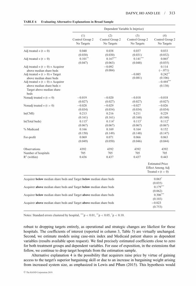
DAFNY, HO AND LEE / 313
TABLE 6 Evaluating Alternative Explanations in Broad Sample
Dependent Variable Is ln(price)
(1) (2) (3) (4)Control Group 2 Control Group 2 Control Group 2 Control Group 2
No Targets No Targets No Targets No Targets
Adj treated ∗ (t = 0) 0.040 0.038 0.037 0.033(0.030) (0.030) (0.031) (0.032)
Adj treated ∗ (t > 0) 0.101** 0.167*** 0.141*** 0.065*
(0.047) (0.063) (0.048) (0.035)Adj treated ∗ (t > 0) ∗ Acquirer
above median share beds−0.092 0.114(0.084) (−.071)
Adj treated ∗ (t > 0) ∗ Targetabove median share beds
−0.085 0.242**
(0.081) (0.106)Adj treated ∗ (t > 0) ∗ Acquirer
above median share beds ∗Target above median sharebeds
−0.444***
(0.138)
Nonadj treated ∗ (t = 0) −0.019 −0.020 −0.018 −0.018(0.027) (0.027) (0.027) (0.027)
Nonadj treated ∗ (t > 0) −0.028 −0.029 −0.027 −0.026(0.034) (0.034) (0.034) (0.034)
ln(CMI) 0.213 0.216 0.211 0.229(0.161) (0.161) (0.160) (0.160)
ln(Total beds) 0.115* 0.114* 0.113* 0.112*
(0.067) (0.067) (0.067) (0.067)% Medicaid 0.166 0.169 0.164 0.152
(0.150) (0.149) (0.148) (0.147)For-profit 0.069 0.071 0.066 0.063
(0.049) (0.050) (0.046) (0.044)
Observations 4392 4392 4392 4392Number of hospitals 705 705 705 705R2 (within) 0.436 0.437 0.437 0.443
Estimated PriceEffect Among AdjTreated ∗ (t > 0)
Acquirer below median share beds and Target below median share beds 0.065*
(0.035)Acquirer above median share beds and Target below median share beds 0.179***
(0.062)Acquirer below median share beds and Target above median share beds 0.306***
(0.103)Acquirer above median share beds and Target above median share beds −0.023
(0.753)
Notes: Standard errors clustered by hospital, ***p < 0.01, **p < 0.05, *p < 0.10.
robust to dropping targets entirely, as operational and strategic changes are likeliest for thesehospitals. The coefficients of interest (reported in column 3, Table 5) are virtually unchanged.Second, we estimate models using case-mix index and Medicaid patient shares as dependentvariables (results available upon request). We find precisely estimated coefficients close to zerofor both treatment groups and dependent variables. For ease of exposition, in the extensions thatfollow, we continue to drop target hospitals from the estimation sample.
Alternative explanation 4 is the possibility that acquirers raise price by virtue of gainingaccess to the target’s superior bargaining skill or due to an increase in bargaining weight arisingfrom increased system size, as emphasized in Lewis and Pflum (2015). This hypothesis would
C© The RAND Corporation 2019.
314 / THE RAND JOURNAL OF ECONOMICS
not explain the stronger effects we see for mergers within 30–90 minutes’ drive, as most insurersoperate statewide. Notwithstanding this observation, we note that our empirical approach probablyskews us away from identifying an effect due to transfer of bargaining skill across hospitals. UnlikeLewis and Pflum (2015), who analyze price effects for stand-alone hospitals that are purchasedby out-of-market systems, our estimation sample focuses on acquiring systems. We explicitlyexclude stand-alone hospitals, as we analyze bystander hospitals to each transaction. Acquiringsystems in our sample are large relative to targets. If bargaining skill is increasing in system size,as Lewis and Pflum (2015) hypothesize, this implies that acquirers in our data are unlikely to gainsubstantial new bargaining skill from the mergers we study.37 Thus, our results can be viewedas complementary to those in Lewis and Pflum (2015). We provide evidence of merger priceincreases consistent with common customer effects, whereas that article focuses on a differentdata sample that highlights the possibility that stand-alone hospitals, when acquired by largesystems, can experience price increases consistent with improved bargaining skill.
Alternative explanation 5 for our results is that they capture horizontal rather than cross-market effects. To evaluate this possibility, we consider two supplemental analyses. First, we usea “same-market” definition of 45 minutes, rather than 30, for the broad sample. The 45-minutedriving radius definition causes many treatment hospitals to be dropped, as we exclude within-market merging hospitals (as well as all hospitals in the control group located within the samedistance of any of these overlapping treatment hospitals). The estimated treatment effect is ofsimilar magnitude (i.e., nearly a 10% price effect using both control groups), suggesting that thecross-market effect is present even when horizontal market boundaries are large—although it isestimated much less precisely (p-values < 0.15). Although it is possible that horizontal effectsimpact a larger geographic area than we allow, these results suggest the price increase is not largerfor hospitals within a 30–45 minute range, that is, those likelier to be substitutes for the same setof patients.
Second, we look directly at whether the hospitals with same-market overlap (i.e., thosewe drop in our main analysis) exhibit price increases. The estimated price effect for hospitalsdropped from the FTC sample due to same-market overlap is small and negative (and statisticallyindistinguishable from zero). We interpret this result as consistent with appropriate enforcementactivity (i.e., either the merger efficiencies outweighed any potential anticompetitive effects orthe hospitals were not close substitutes ex ante), or with the possibility that the scrutiny of variousstakeholders impacted post-merger price negotiations. In the broad sample, we note that onlyfive hospitals exist in the “horizontal overlap” group, because the median target system size isone and we always exclude the largest target hospital from our analysis. Among these five, weobserve a price increase, but only in the year of acquisition. After this year, price is no longerstatistically different from the pre-merger years. Given the small sample size, we are loath to drawconclusions from this analysis.38
6. Concluding remarks
� This study provides theoretical and empirical analyses of the price effects of cross-marketmergers of upstream suppliers to intermediaries who bundle and sell their services. Our modelemphasizes the ways in which cross-market mergers differ from within-market mergers, setting
37 Lewis and Pflum (2015) reports that, for every 10 additional hospital members of a (not-for-profit) hospitalsystem, the members extract an additional 8%–9% of surplus from their contracts with insurers. Assuming no change incosts, the implied impact on acquirer price of the modal acquisition (one hospital) is 0.8%–0.9%, a figure much smallerthan our estimated 10% price effect on acquirers.
38 Our sample is not designed to study the effects of same-market overlap, and these results should not be viewedas inconsistent with the large literature that finds mergers of close substitutes in the same patient market yield substantialprice increases. In particular, we do not include any one-to-one mergers as they lack bystanders, and we require mergingparties to engage in only one such transaction (nationwide) over a given five-year period so that we can have a clearpre-and post-treatment period. Our results likely also reflect our crude horizontal market definition, as well as appropriateenforcement activity.
C© The RAND Corporation 2019.
DAFNY, HO AND LEE / 315
aside commonalities shared across both merger types—such as changes in bargaining skill,managerial practices, service mix, and costs. The theory demonstrates that price changes (bothpositive and negative) may arise when the merging parties negotiate with a common buyer, andcustomers of that buyer value both parties (i.e., their demand for the bundle is influenced by theinclusion of the parties). We also discuss alternative explanations for how prices can change evenabsent these common customers.
Using data on two distinct samples of transactions—and focusing on “bystander” hospitalsthat are not likely to be the drivers of the transactions and are thus arguably exogenously treated—we compare price effects of gaining a system member in-state versus out-of-state. We findthat hospitals acquiring another system member in-state raise price by 7%–10%, whereas anacquisition out-of-state does not result in a statistically meaningful change in price. Furtheranalyses provide suggestive evidence that mergers of proximate hospitals (i.e., within 30–90minutes’ drive, in-state) lead to the largest price effects. These are precisely the sort of cross-market hospital mergers where common customers are likeliest to be present. We interpret theseresults as consistent with the presence of a common customer effect that is driving post-mergerprice increases. We also show the results are similar when dropping target hospitals, whichsuggests that changes to a target’s operations are not the driver of the estimated price effects. Last,we find no changes in case mix or Medicaid patient share for acquirers, as might be expected ifacquirers reposition themselves in terms of services offered and customer segments.
Prior researchers have shown that mergers of nearby, similar rivals can lead to increases inmarket power and higher prices. The existence of a common customer effect implies that marketpower may arise from combinations over even broader geographic areas and across productmarkets. This finding does not imply more expansive boundaries for mechanical calculations ofmarket shares and “change in Herfindahl-Hirschman Index” s used to evaluate whether mergersare likely to be anticompetitive; rather, we believe it favors an emphasis on the “direct effects”likely to arise from a merger, a concept promulgated in the 2010 Horizontal Merger Guidelines.The results do suggest that combinations across broader areas should be carefully evaluatedby antitrust authorities, particularly if customers (such as employers) value insurance productscontaining both merging parties, if there is significant commuting between the areas where themerging parties are located, and/or if the same insurers are dominant.
Cross-market mergers are an increasingly relevant phenomenon in the United States, andparticularly in the healthcare landscape. The theoretical and empirical analyses in this studyillustrate that at least some of the mechanisms by which cross-market hospital mergers generateprice increases are related to a diminution of competition among the merging parties for inclusionin insurer networks, and are therefore relevant for antitrust enforcement. Additional research thatexplicitly models the links between and among insurance choice, insurance competition, andhospital-insurer bargaining could prove valuable to antitrust enforcers and others interested infostering and protecting competition in healthcare markets.
Appendix A
This appendix contains additional details regarding our theoretical analyses.
A.1 Willingness-to-Pay (WTP) for an insurer’s network. In this section, we define the “willingness-to-pay” of anindividual for the insurer’s network of hospitals G, represented by W T P(G). WTP is typically used as an argument in theinsurer’s objective function � when the insurer bargains with hospitals.
The literature (e.g., Town and Vistnes, 2001; Capps, Dranove, and Satterthwaite, 2003; Ho, 2006) derives WTPfrom a simple model of individual demand for hospitals typically as follows. Suppose that the utility of a given individualp from visiting hospital i given diagnosis l is:
u p,i,l = δi + zi υp,lβ + εp,i,l ,
where δi is the average quality of the hospital, zi υp,l are interactions between observed hospital and individual character-istics (which may vary by diagnosis l), and εp,i,l is an i.i.d. logit error term. This model generates a simple expression forindividual p’s expected utility from the hospitals in the insurer’s network for diagnosis l (EU p,i,l ). These values are then
C© The RAND Corporation 2019.
316 / THE RAND JOURNAL OF ECONOMICS
weighted by the probability that individual p is admitted to a hospital and diagnosed with l (γp,l ) to obtain the expectedWTP for that individual:
WTPp(G) =∑
l
γp,l EU p,i,l (G). (A1)
Furthermore, we denote by �WTPp(G, h) ≡ WTPp(G) − WTPp(G \ h) the change in individual p’s WTP for an insurer’snetwork if that insurer loses access to hospital h. Similarly, we define �WTPp(G,S) for any hospital system S.
Merger effects on �WTP. First, note that if h1 and h2 compete for the same individual within the same geographicmarket m and diagnosis l, it will generally be the case (e.g., with logit utility for hospitals) that:
�WTPp(G,S) >∑
h∈{h1 ,h2}�WTPp(G, h), (A2)
where S ≡ {1, 2}. This arises from the nonlinearity in EU p,i,l and substitutability of the hospitals. For intuition, notethat if the insurer drops only hospital 1, this may reduce WTP very little because customers can substitute to hospital 2;however, if the two hospitals merge, and there is no other close substitute in the market, dropping the combined hospitalsystem S reduces customer WTP by a greater amount. Thus, the impact of the loss of hospital 1 to the WTP for an insurer’snetwork will be greater if 2 is also absent from the network if hospitals 1 and 2 are substitutes (Capps, Dranove, andSatterthwaite, 2003).
However, if hospitals 1 and 2 do not compete for the same individual—either because the hospitals are located indifferent geographic markets or because they serve different diagnoses—then (A2) will not hold. Instead, it will be thecase that �WTPp(G,S) = ∑
h∈{h1 ,h2} �WTPp(G, h) and the change in an insurer’s WTP from losing both hospitals willsimply be the sum of the change in the insurer’s WTP from losing each individual hospital.
A.2 Insurance demand with cross-market price effects. In the fourth subsection of Section 2, we note that ifhouseholds, rather than individuals, choose insurers based on a utility equation that includes the sum of householdmembers’ WTP for the hospital network, this may generate links across diagnostic markets that can generate price effectsof cross-diagnostic market hospital mergers. We now provide another example.
Assume an insurer’s objective function is equal to its profits, and that profits can be represented by � = D(·) ×(φ − η), where D is the demand for the insurer’s product, and φ and η are per-enrollee premiums and insurer nonhospitalcosts.39 Assume in addition, for ease of exposition, that the margin per enrollee is invariant to the negotiated hospitalnetwork. Substituting this formulation for � into our necessary condition for a hospital merger to have a positive priceeffect (6) yields:
[D(G) − D(G \ S)] >∑
h∈{h1 ,h2}D(G) − D(G \ h), (A3)
(where, if the inequality were reversed, the price effect would be negative). Thus, a sufficient condition for hospitals h1
and h2 to benefit from a merger despite being in different (geographic or product) markets would be for the change indemand for the insurer when both hospitals are dropped together to exceed the sum of changes in enrollment when eachis dropped individually.
The “concavity” of demand for an insurer’s product in the utility generated by its network, represented by (A3), canarise whenever the merging hospitals have one or more common customers. Consider a stylized setting where an insurercompetes against an outside option (e.g., not purchasing insurance or purchasing plans offered by other insurers). Thisinsurer delivers utility to customer c given by v = g(·) + W T Pc(G), where g(·) is some function of insurer and marketcharacteristics. Furthermore, assume that the insurer has captive enrollees who would not switch to the outside option(which delivers some utility v0) unless they are subjected to a reduction in utility that is large enough to outweigh theswitching costs. In this case, if only hospital i or k were dropped by the insurer, a customer may not find it worthwhileto leave the insurer, and thus the insurer’s loss in profits from disagreement with either i or k would be minimal. If,however, both hospitals were excluded from the insurer’s network, then customers may find it worthwhile to switch to acompeting insurer (or outside option). Thus, the presence of switching costs may also generate the necessary concavityin the insurer’s objective function.
Whether (6) holds will depend not only on the properties of demand for insurers, but also on how the margins perenrollee are determined (which, for simplicity, we have assumed fixed). Adding these considerations or other complexities(e.g., choice set variation, informational frictions, etc.) to the model may change the precise behavior of D, but are unlikelyto restore the linearity of the insurer’s objective (�) in the utility of its network (WTP). More generally, we observe thatmoving from the simple linear insurer objective function assumed in earlier models to a more realistic function reflectinginsurer profits generates non linearities in WTP quite easily, and this is all that is needed for cross-market price effects(the direction of which, as noted in the main text, is theoretically ambiguous).
39 Ho and Lee (2017) contains a general analysis of this type of model.
C© The RAND Corporation 2019.
DAFNY, HO AND LEE / 317
A.3 Caveats and limiting factors. We note in the fifth subsection of Section 2 that common customer effects wouldnot arise under some amended versions of the model. We now provide details of three such situations.
Inelastic insurer demand with respect to the network. A key component of the common customer effect in the hospital-insurer setting is the large reduction in the insurer’s profits if it loses the merged hospital system (relative to losing eachhospital separately). In our example, this arose from an increased likelihood that employers would switch to other insurers.In settings, both within and outside of healthcare, where dropping an upstream merged entity is unlikely to affect thedownstream intermediary’s demand, there may be no price effects of cross-market mergers.40
Separable demand by common customers. The simple model also assumed that employers faced a cost of offeringadditional plans. If instead, employers could costlessly offer different plans in different markets, then markets would againbe separable and no cross-market merger price effects would arise. However, insurers commonly design plans to coverbroader geographic areas than most hospital service markets (Vistnes and Sarafidis, 2013), making this disaggregationdifficult. We also note the empirical regularity that employers seem to prefer one-stop shopping. For example, CalPERS, anagency which provides pension and health benefits to California state and public employees, retirees, and their dependents,offers a single menu of plans across most markets in California.
Separable bargaining. Our model assumes that hospital systems bargain jointly with each insurer. If systems bargainhospital by hospital, that is, they cannot impose “all or nothing” requirements on insurers, then again, the cross-marketprice effects will be removed. Anecdotal evidence, and estimates in articles such as Ho (2009) and Lewis and Pflum (2015),suggest that systems generally negotiate jointly, and often require insurers to include all system members in contracts.
A.4 “Common insurer” effects with no common customer. The sixth subsection of Section 2 outlines two situationswhere cross-market hospital mergers can generate price effects due to the presence of common insurers, even thoughthere are no customers who value both merging hospitals. We now provide details of these mechanisms.
Price cap in one market. Consider a setting in which there is an independent hospital subject to a price cap due topolitical or regulatory restrictions. Suppose the cap binds so that the hospital is unable to increase its price to the levelimplied by Nash bargaining. In our model, this would imply that the first-order condition given by (2) is slack, and that theLHS of (2) is strictly less than the RHS. Consider now the effect of a merger between this hospital and another in a secondmarket that is not subject to a price cap. If there is a common insurer that negotiates with both hospitals, (5) implies thatthe sum of the hospital prices will be a function of the hospital system’s contributions to the insurer’s revenues. As aresult, by merging, the hospital subject to the price cap can generate an increase in the second hospital’s negotiated pricesso that the merged hospital system’s Nash bargaining first-order condition given by (5) will bind. Thus, the merger canyield a price effect due to the presence of a common insurer, even if the hospitals that merged were never valued by thesame customers.
Linear prices and double marginalization. Now consider a scenario where a monopolist insurer is active in two marketsA and B, there are monopolist hospitals active in each market, and negotiated prices are linear (i.e., per-patient payments).Assume that the insurer’s profit in each market m ∈ {A, B}, if it has an agreement with the hospital in the market, is givenby �m = Dm(φm) × (φm − pm), where Dm represents the demand for the insurer, φm is the insurer’s premiums, and pm isnow a (linear) per-enrollee price negotiated with the hospital in that market for hospital services.41 Thus, each hospital’sprofit upon agreement is given by πm = Dm pm . For simplicity, we assume away fixed and marginal costs; including themwill not change the result. We also assume that the insurer and hospital in each market do not obtain any demand or profitswithout agreeing to a contract: that is, the disagreement point from bargaining for both parties is 0.
Finally, we assume that premiums are set in each market after bargaining over hospital prices concludes. Thus, thepremiums that the insurer sets in each market will satisfy:
φ∗m = argmax
φ
Dm(φ)(φ − pm). (A4)
If the hospitals are not merged, prices in each market are assumed to satisfy the following asymmetric Nash bargain:
p∗m = argmax
p[Dm(φ∗
m(p))(φ∗m(p) − p)]1−b × [Dm(φ∗
m(p))p]b m ∈ {A, B}, (A5)
40 A dominant insurer negotiating with relatively small physician groups who are merging may be one example.Another may be the merger between Proctor & Gamble and Gillette: although the two companies did not primarilycompete with one another in any given product market, their merger may have provided them with an ability to negotiatebetter terms with retailers offering “one-stop” shopping services to households. However, it is plausible that consumerswould not switch away from major retailers even if both firms’ products were removed from its shelves, implying noincrease in bargaining leverage, and no merger price effect.
41 For exposition and to simplify notation, we assume that the hospital is paid for all enrollees. Assuming that onlysome fraction of enrollees visit the hospital, and that the hospital is reimbursed only for those enrollees that visit, doesnot affect the spirit of the following analysis.
C© The RAND Corporation 2019.
318 / THE RAND JOURNAL OF ECONOMICS
where φ∗m(p) represents the solution to (A4) for a given negotiated price p. The first order condition of (A5) can be
expressed as:
�m pm
Dm(·) = pm − bφ∗m(p)
b(φ∗m(p) − pm)
m ∈ {A, B}, (A6)
where �m = (∂ Dm/∂φm)(∂φm/∂pm) and represents the change in the insurer’s demand due to an increase in its premiumsbrought on by an increase in the negotiated price (i.e., the effect on demand of pass-through).
On the other hand, if the two hospitals merge and prices are jointly negotiated to maximize:
{pM,∗A , pM,∗
B } = argmaxpA ,pB
[DA(·)(φ∗A(pA) − pA) + DB (·)(φ∗
B (pB ) − pB )]1−b × [(DA(·)pA + DB (·)pB )]b, (A7)
then the FOCs of (A7) can be expressed as:
�A pA
DA(·) = �B pB
DB (·) = [(DA(·)(pA − bφ∗A(pA)) + DB (·)(pB − bφ∗
B (pB ))]
b[DA(·)(φ∗A(pA) − pA) + DB (·)(φ∗
B (pB ) − pB )]. (A8)
The left-hand sides of both (A6) and (A8) correspond to the elasticity of (insurer) demand with respect to thenegotiated price. Consider two cases:
1. If � = 0 so that these elasticities are 0—as in the case where premiums are set before or simultaneously withnegotiated prices, or prices are lump-sums as opposed to linear—then the prices that satisfy the nonmerged Nashbargaining FOCs given by (A6) would also satisfy the merged Nash bargaining FOCs in (A8). In such a setting,without a merger, prices in each market would be p∗
m = bφ∗m , that is, negotiated prices would be a fraction b of the
fixed premiums; with a merger, prices∑
m Dm p∗m = b
∑m Dmφ∗
m , that is, total payments to the merged entity wouldbe the same fraction b of total insurer revenues across both markets. Although a merger could thus result in a changein prices across markets (higher in one, lower in another), total payments to the hospitals would be unchanged andthere would be no merger price effects (although distributional effects may arise).
2. On the other hand, if �m �= 0—which generally will be the case when premiums are set after linear fees are ne-gotiated42—the total prices that are negotiated to satisfy (A6) need not be the same as those negotiated to satisfy(A8). Note that the merged Nash bargaining FOC in (A8) requires that the elasticities of demand with respect to thenegotiated prices across both markets m ∈ {A, B} are equalized, whereas this need not be the case absent a merger.Indeed, insofar as an inefficiency is introduced (from the perspective of the insurer and hospitals) by the doublemarginalization arising from the insurer’s markup of the hospitals’ negotiated prices, there are potential industry profitgains from having a hospital system internalize the pricing effects across markets. For example, if the magnitude ofthe elasticity of demand with respect to p∗
A (in market A) is greater than the elasticity of demand with respect to p∗B
(in market B), so that a price increase in market A would lead to a larger reduction in demand than in market Bat the negotiated prices when the hospitals are independent, then a merged hospital system would wish to adjust itsprices to set a lower pM,∗
A < p∗A and offset this with a higher pM,∗
B > p∗B . Due to the increase in industry surplus from
internalizing these cross-market differences, a hospital merger can increase the total payments made to the hospitalsystem.
The key to generating this type of cross-market merger price effect absent a common customer is the existence ofan inefficiency from the perspective of the bargaining firms—that is, double marginalization due to linear fees. Mitigatingthis inefficiency via a hospital merger can leave both the hospitals and the insurer better off. The harm to customers willdiffer across markets, with those facing lower premiums as a result of lower negotiated prices benefiting from the merger.
Though this stand-alone common insurer effect may be relevant in some cases, we conjecture that it is lessempirically relevant than the common customer effect (which presumes a common insurer). First, for this particular effectto obtain, hospitals must be paid linear fees rather than two-part tariffs. Second, premium-setting must lag behind pricenegotiations sufficiently for premiums to be set in response to prices. Either assumption may fail in particular markets.Finally, the double marginalization effect may result in a weighted average decrease in hospital prices; empirically, weobserve an increase.
Appendix B
This appendix contains further information on our empirical analysis.
B.1 The price variable. We construct an estimate of hospital-year private prices using the Healthcare Cost ReportInformation System (HCRIS) data set for fiscal years 1996–2012. HCRIS is a public data set gathered by the Centersfor Medicare and Medicaid Services (CMS). We follow the methodology in Dafny (2009), calculating private price asthe (estimated) net revenue for non-Medicare inpatient admissions, divided by the number of non-Medicare admissions.
42 Insurance regulators require substantial documentation of expected medical spending to ensure the solvency ofinsurers. These projections ordinarily reflect provider rates and expected utilization.
C© The RAND Corporation 2019.
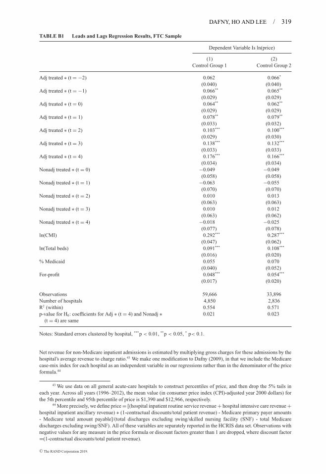
DAFNY, HO AND LEE / 319
TABLE B1 Leads and Lags Regression Results, FTC Sample
Dependent Variable Is ln(price)
(1) (2)Control Group 1 Control Group 2
Adj treated ∗ (t = −2) 0.062 0.066*
(0.040) (0.040)Adj treated ∗ (t = −1) 0.066** 0.065**
(0.029) (0.029)Adj treated ∗ (t = 0) 0.064** 0.062**
(0.029) (0.029)Adj treated ∗ (t = 1) 0.078** 0.079**
(0.033) (0.032)Adj treated ∗ (t = 2) 0.103*** 0.100***
(0.029) (0.030)Adj treated ∗ (t = 3) 0.138*** 0.132***
(0.033) (0.033)Adj treated ∗ (t = 4) 0.176*** 0.166***
(0.034) (0.034)Nonadj treated ∗ (t = 0) −0.049 −0.049
(0.058) (0.058)Nonadj treated ∗ (t = 1) −0.063 −0.055
(0.070) (0.070)Nonadj treated ∗ (t = 2) 0.010 0.013
(0.063) (0.063)Nonadj treated ∗ (t = 3) 0.010 0.012
(0.063) (0.062)Nonadj treated ∗ (t = 4) −0.018 −0.025
(0.077) (0.078)ln(CMI) 0.292*** 0.287***
(0.047) (0.062)ln(Total beds) 0.091*** 0.108***
(0.016) (0.020)% Medicaid 0.055 0.070
(0.040) (0.052)For-profit 0.048*** 0.054***
(0.017) (0.020)
Observations 59,666 33,896Number of hospitals 4,850 2,836R2 (within) 0.554 0.571p-value for H0: coefficients for Adj ∗ (t = 4) and Nonadj ∗
(t = 4) are same0.021 0.023
Notes: Standard errors clustered by hospital, ***p < 0.01, **p < 0.05, * p< 0.1.
Net revenue for non-Medicare inpatient admissions is estimated by multiplying gross charges for these admissions by thehospital’s average revenue to charge ratio.43 We make one modification to Dafny (2009), in that we include the Medicarecase-mix index for each hospital as an independent variable in our regressions rather than in the denominator of the priceformula.44
43 We use data on all general acute-care hospitals to construct percentiles of price, and then drop the 5% tails ineach year. Across all years (1996–2012), the mean value (in consumer price index (CPI)-adjusted year 2000 dollars) forthe 5th percentile and 95th percentile of price is $1,390 and $12,966, respectively.
44 More precisely, we define price = [(hospital inpatient routine service revenue + hospital intensive care revenue +hospital inpatient ancillary revenue) ∗ (1-contractual discounts/total patient revenue) - Medicare primary payer amounts- Medicare total amount payable]/(total discharges excluding swing/skilled nursing facility (SNF) - total Medicaredischarges excluding swing/SNF). All of these variables are separately reported in the HCRIS data set. Observations withnegative values for any measure in the price formula or discount factors greater than 1 are dropped, where discount factor=(1-contractual discounts/total patient revenue).
C© The RAND Corporation 2019.
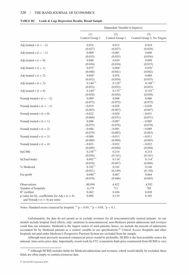
320 / THE RAND JOURNAL OF ECONOMICS
TABLE B2 Leads & Lags Regression Results, Broad Sample
Dependent Variable Is ln(price)
(1) (2) (3)Control Group 1 Control Group 2 Control Group 2, No Targets
Adj treated ∗ (t = −2) 0.016 0.013 0.018(0.027) (0.027) (0.029)
Adj treated ∗ (t = −1) 0.009 −0.001 0.009(0.035) (0.035) (0.036)
Adj treated ∗ (t = 0) 0.040 0.039 0.049(0.034) (0.034) (0.035)
Adj treated ∗ (t = 1) 0.075* 0.068* 0.076*
(0.040) (0.041) (0.042)Adj treated ∗ (t = 2) 0.094* 0.076 0.089
(0.053) (0.054) (0.055)Adj treated ∗ (t = 3) 0.144*** 0.128** 0.148***
(0.053) (0.052) (0.053)Adj treated ∗ (t = 4) 0.144** 0.135** 0.143**
(0.058) (0.058) (0.058)Nonadj treated ∗ (t = −2) 0.009 0.008 0.006
(0.073) (0.075) (0.075)Nonadj treated ∗ (t = −1) −0.019 −0.028 −0.030
(0.065) (0.067) (0.067)Nonadj treated ∗ (t = 0) −0.022 −0.028 −0.031
(0.068) (0.071) (0.071)Nonadj treated ∗ (t = 1) 0.000 −0.007 −0.005
(0.075) (0.078) (0.078)Nonadj treated ∗ (t = 2) −0.084 −0.091 −0.089
(0.079) (0.083) (0.083)Nonadj treated ∗ (t = 3) −0.000 −0.015 −0.011
(0.089) (0.094) (0.095)Nonadj treated ∗ (t = 4) −0.033 −0.032 −0.032
(0.089) (0.094) (0.094)ln(CMI) 0.258*** 0.214 0.214
(0.056) (0.161) (0.161)ln(Total beds) 0.092*** 0.116* 0.114*
(0.018) (0.067) (0.068)% Medicaid 0.102** 0.162 0.166
(0.051) (0.149) (0.150)For-profit 0.040** 0.067 0.064
(0.019) (0.046) (0.045)
Observations 40,994 4,422 4,392Number of hospitals 4,174 711 705R2 (within) 0.462 0.436 0.438p-value for H0: coefficients for Adj ∗ (t = 4)
and Nonadj ∗ (t = 4) are same0.096 0.119 0.103
Notes: Standard errors clustered by hospital, ***p < 0.01, **p < 0.05, *p < 0.1.
Unfortunately, the data do not permit us to exclude revenues for all noncommercially insured patients. As ourmodels include hospital fixed effects, only variations in noncommercial, non-Medicare patient admissions and revenuescould bias our estimates. Medicaid is the largest source of such patients, hence, we include the percent of admissionsaccounted for by Medicaid patients as a control variable in our specifications.45 Critical Access Hospitals and otherhospitals not paid under Medicare’s Prospective Payment System are excluded from the sample.
Although more precisely measured commercial prices would be preferable, HCRIS is the best-available source fornational, time-series price data. Importantly, recent work by FTC economists finds price constructed from HCRIS is very
45 Although HCRIS includes fields for Medicaid admissions and revenues, which would ideally be excluded, thesefields are often empty or contain erroneous data.
C© The RAND Corporation 2019.
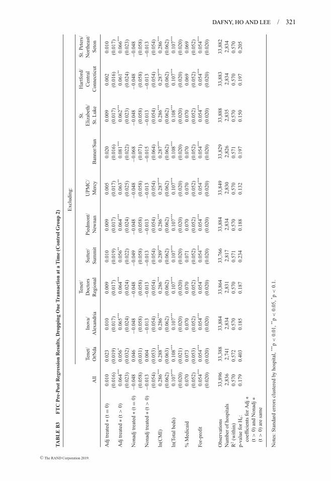
DAFNY, HO AND LEE / 321
TA
BL
EB
3F
TC
Pre
-Pos
tR
egre
ssio
nR
esul
ts,D
ropp
ing
One
Tra
nsac
tion
ata
Tim
e(C
ontr
olG
roup
2)
Exc
ludi
ng:
All
Tene
t/O
rNda
Inov
a/A
lexa
ndri
a
Tene
t/D
octo
rsR
egio
nal
Sut
ter/
Sum
mit
Pie
dmon
t/N
ewna
nU
PM
C/
Mer
cyB
anne
r/S
un
St.
Eli
zabe
th/
St.
Luk
e
Har
tfor
d/C
entr
alC
onne
ctic
ut
St.
Pete
rs/
Nor
thea
st/
Set
on
Adj
trea
ted
∗(t=
0)0.
010
0.02
30.
010
0.00
90.
010
0.00
90.
005
0.02
00.
009
0.00
20.
010
(0.0
16)
(0.0
19)
(0.0
17)
(0.0
17)
(0.0
19)
(0.0
17)
(0.0
17)
(0.0
16)
(0.0
17)
(0.0
16)
(0.0
17)
Adj
trea
ted
∗(t>
0)0.
064**
*0.
056*
0.06
5***
0.06
4***
0.05
6**0.
064**
*0.
063**
0.08
1***
0.06
2***
0.06
1**0.
066**
*
(0.0
23)
(0.0
32)
(0.0
24)
(0.0
24)
(0.0
22)
(0.0
24)
(0.0
25)
(0.0
22)
(0.0
23)
(0.0
24)
(0.0
23)
Non
adjt
reat
ed∗(
t=0)
−0.0
480.
046
−0.0
48−0
.048
−0.0
49−0
.048
−0.0
48−0
.068
−0.0
48−0
.048
−0.0
48(0
.058
)(0
.031
)(0
.058
)(0
.058
)(0
.058
)(0
.058
)(0
.058
)(0
.071
)(0
.058
)(0
.058
)(0
.058
)N
onad
jtre
ated
∗(t>
0)−0
.013
0.00
4−0
.013
−0.0
13−0
.013
−0.0
13−0
.013
−0.0
15−0
.013
−0.0
13−0
.013
(0.0
54)
(0.0
53)
(0.0
54)
(0.0
54)
(0.0
54)
(0.0
54)
(0.0
54)
(0.0
64)
(0.0
54)
(0.0
54)
(0.0
54)
ln(C
MI)
0.28
6***
0.28
8***
0.28
6***
0.28
6***
0.28
9***
0.28
6***
0.28
7***
0.28
7***
0.28
6***
0.28
7***
0.28
6***
(0.0
62)
(0.0
63)
(0.0
62)
(0.0
62)
(0.0
62)
(0.0
62)
(0.0
62)
(0.0
62)
(0.0
62)
(0.0
62)
(0.0
62)
ln(T
otal
beds
)0.
107**
*0.
108**
*0.
107**
*0.
107**
*0.
107**
*0.
107**
*0.
107**
*0.
108**
*0.
108**
*0.
107**
*0.
107**
*
(0.0
20)
(0.0
21)
(0.0
20)
(0.0
20)
(0.0
20)
(0.0
20)
(0.0
20)
(0.0
20)
(0.0
20)
(0.0
20)
(0.0
20)
%M
edic
aid
0.07
00.
073
0.07
00.
070
0.07
10.
070
0.07
00.
070
0.07
00.
069
0.06
9(0
.052
)(0
.053
)(0
.052
)(0
.052
)(0
.052
)(0
.052
)(0
.052
)(0
.052
)(0
.052
)(0
.052
)(0
.052
)Fo
r-pr
ofit
0.05
4***
0.05
4***
0.05
4***
0.05
4***
0.05
4***
0.05
4***
0.05
4***
0.05
4***
0.05
4***
0.05
4***
0.05
4***
(0.0
20)
(0.0
20)
(0.0
20)
(0.0
20)
(0.0
20)
(0.0
20)
(0.0
20)
(0.0
20)
(0.0
20)
(0.0
20)
(0.0
20)
Obs
erva
tion
s33
,896
33,3
8833
,884
33,8
6433
,766
33,8
8433
,849
33,8
2933
,888
33,8
8333
,882
Num
ber
ofho
spit
als
2,83
62,
741
2,83
42,
831
2,81
72,
834
2,83
02,
826
2,83
52,
834
2,83
4R
2(w
ithi
n)0.
570
0.57
20.
570
0.57
00.
571
0.57
00.
570
0.57
10.
570
0.57
00.
570
p-va
lue
for
H0:
coef
fici
ents
for
Adj
∗(t
>0)
and
Non
adj∗
(t>
0)ar
esa
me
0.17
90.
403
0.18
50.
187
0.23
40.
188
0.13
20.
197
0.15
00.
197
0.20
5
Not
es:S
tand
ard
erro
rscl
uste
red
byho
spit
al,**
*p
<0.
01,**
p<
0.05
,*p
<0.
1.
C© The RAND Corporation 2019.
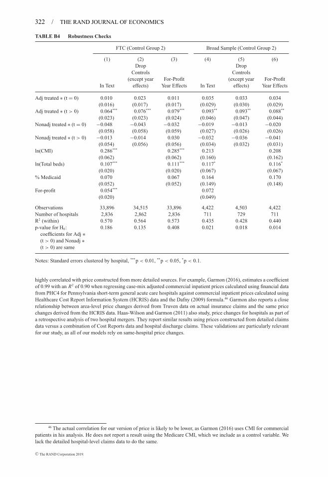
322 / THE RAND JOURNAL OF ECONOMICS
TABLE B4 Robustness Checks
FTC (Control Group 2) Broad Sample (Control Group 2)
(1) (2) (3) (4) (5) (6)
In Text
DropControls
(except yeareffects)
For-ProfitYear Effects In Text
DropControls
(except yeareffects)
For-ProfitYear Effects
Adj treated ∗ (t = 0) 0.010 0.023 0.011 0.035 0.033 0.034(0.016) (0.017) (0.017) (0.029) (0.030) (0.029)
Adj treated ∗ (t > 0) 0.064*** 0.076*** 0.079*** 0.093** 0.093** 0.088**
(0.023) (0.023) (0.024) (0.046) (0.047) (0.044)Nonadj treated ∗ (t = 0) −0.048 −0.043 −0.032 −0.019 −0.013 −0.020
(0.058) (0.058) (0.059) (0.027) (0.026) (0.026)Nonadj treated ∗ (t > 0) −0.013 −0.014 0.030 −0.032 −0.036 −0.041
(0.054) (0.056) (0.056) (0.034) (0.032) (0.031)ln(CMI) 0.286*** 0.285*** 0.213 0.208
(0.062) (0.062) (0.160) (0.162)ln(Total beds) 0.107*** 0.111*** 0.117* 0.116*
(0.020) (0.020) (0.067) (0.067)% Medicaid 0.070 0.067 0.164 0.170
(0.052) (0.052) (0.149) (0.148)For-profit 0.054*** 0.072
(0.020) (0.049)
Observations 33,896 34,515 33,896 4,422 4,503 4,422Number of hospitals 2,836 2,862 2,836 711 729 711R2 (within) 0.570 0.564 0.573 0.435 0.428 0.440p-value for H0:
coefficients for Adj ∗(t > 0) and Nonadj ∗(t > 0) are same
0.186 0.135 0.408 0.021 0.018 0.014
Notes: Standard errors clustered by hospital, ***p < 0.01, **p < 0.05, *p < 0.1.
highly correlated with price constructed from more detailed sources. For example, Garmon (2016), estimates a coefficientof 0.99 with an R2 of 0.90 when regressing case-mix adjusted commercial inpatient prices calculated using financial datafrom PHC4 for Pennsylvania short-term general acute care hospitals against commercial inpatient prices calculated usingHealthcare Cost Report Information System (HCRIS) data and the Dafny (2009) formula.46 Garmon also reports a closerelationship between area-level price changes derived from Truven data on actual insurance claims and the same pricechanges derived from the HCRIS data. Haas-Wilson and Garmon (2011) also study, price changes for hospitals as part ofa retrospective analysis of two hospital mergers. They report similar results using prices constructed from detailed claimsdata versus a combination of Cost Reports data and hospital discharge claims. These validations are particularly relevantfor our study, as all of our models rely on same-hospital price changes.
46 The actual correlation for our version of price is likely to be lower, as Garmon (2016) uses CMI for commercialpatients in his analysis. He does not report a result using the Medicare CMI, which we include as a control variable. Welack the detailed hospital-level claims data to do the same.
C© The RAND Corporation 2019.

DAFNY, HO AND LEE / 323
TABLE B5 Broad Sample, Effects By Minimum Distance between Merging, Adjacent Hospitals
(1)Control Group 2
Adj treated ∗ (30–90) ∗ (t = −2) 0.004(0.038)
Adj treated ∗ (30–90) ∗ (t = −1) −0.019(0.048)
Adj treated ∗ (30–90) ∗ (t = 0) 0.068*
(0.040)Adj treated ∗ (30–90) ∗ (t = 1) 0.085*
(0.048)Adj treated ∗ (30–90) ∗ (t = 2) 0.093
(0.066)Adj treated ∗ (30–90) ∗ (t = 3) 0.149**
(0.061)Adj treated ∗ (30–90) ∗ (t = 4) 0.192***
(0.069)Adj treated ∗ (>90) ∗ (t = −2) 0.029
(0.028)Adj treated ∗ (>90) ∗ (t = −1) 0.032
(0.040)Adj treated ∗ (>90) ∗ (t = 0) −0.019
(0.054)Adj treated ∗ (>90) ∗ (t = 1) 0.031
(0.069)Adj treated ∗ (>90) ∗ (t = 2) 0.041
(0.085)Adj treated ∗ (>90) ∗ (t = 3) 0.082
(0.091)Adj treated ∗ (>90) ∗ (t = 4) 0.033
(0.086)Nonadj treated ∗ (t = −2) 0.008
(0.075)Nonadj treated ∗ (t = −1) −0.027
(0.067)Nonadj treated ∗ (t = 0) −0.027
(0.071)Nonadj treated ∗ (t = 1) −0.007
(0.078)Nonadj treated ∗ (t = 2) −0.090
(0.083)Nonadj treated ∗ (t = 3) −0.015
(0.094)Nonadj treated ∗ (t = 4) −0.032
(0.094)ln(CMI) 0.206
(0.160)ln(Total beds) 0.118*
(0.068)% Medicaid 0.156
(0.147)For-profit 0.063
(0.043)
Observations 4422Number of hospitals 711R2 (within) 0.438
C© The RAND Corporation 2019.
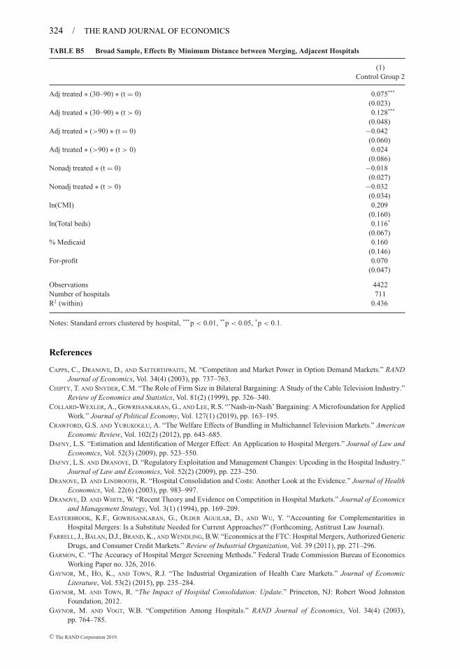
324 / THE RAND JOURNAL OF ECONOMICS
TABLE B5 Broad Sample, Effects By Minimum Distance between Merging, Adjacent Hospitals
(1)Control Group 2
Adj treated ∗ (30–90) ∗ (t = 0) 0.075***
(0.023)Adj treated ∗ (30–90) ∗ (t > 0) 0.128***
(0.048)Adj treated ∗ (>90) ∗ (t = 0) −0.042
(0.060)Adj treated ∗ (>90) ∗ (t > 0) 0.024
(0.086)Nonadj treated ∗ (t = 0) −0.018
(0.027)Nonadj treated ∗ (t > 0) −0.032
(0.034)ln(CMI) 0.209
(0.160)ln(Total beds) 0.116*
(0.067)% Medicaid 0.160
(0.146)For-profit 0.070
(0.047)
Observations 4422Number of hospitals 711R2 (within) 0.436
Notes: Standard errors clustered by hospital, ***p < 0.01, **p < 0.05, *p < 0.1.
References
CAPPS, C., DRANOVE, D., AND SATTERTHWAITE, M. “Competiton and Market Power in Option Demand Markets.” RANDJournal of Economics, Vol. 34(4) (2003), pp. 737–763.
CHIPTY, T. AND SNYDER, C.M. “The Role of Firm Size in Bilateral Bargaining: A Study of the Cable Television Industry.”Review of Economics and Statistics, Vol. 81(2) (1999), pp. 326–340.
COLLARD-WEXLER, A., GOWRISANKARAN, G., AND LEE, R.S. “’Nash-in-Nash’ Bargaining: A Microfoundation for AppliedWork.” Journal of Political Economy, Vol. 127(1) (2019), pp. 163–195.
CRAWFORD, G.S. AND YURUKOGLU, A. “The Welfare Effects of Bundling in Multichannel Television Markets.” AmericanEconomic Review, Vol. 102(2) (2012), pp. 643–685.
DAFNY, L.S. “Estimation and Identification of Merger Effect: An Application to Hospital Mergers.” Journal of Law andEconomics, Vol. 52(3) (2009), pp. 523–550.
DAFNY, L.S. AND DRANOVE, D. “Regulatory Exploitation and Management Changes: Upcoding in the Hospital Industry.”Journal of Law and Economics, Vol. 52(2) (2009), pp. 223–250.
DRANOVE, D. AND LINDROOTH, R. “Hospital Consolidation and Costs: Another Look at the Evidence.” Journal of HealthEconomics, Vol. 22(6) (2003), pp. 983–997.
DRANOVE, D. AND WHITE, W. “Recent Theory and Evidence on Competition in Hospital Markets.” Journal of Economicsand Management Strategy, Vol. 3(1) (1994), pp. 169–209.
EASTERBROOK, K.F., GOWRISANKARAN, G., OLDER AGUILAR, D., AND WU, Y. “Accounting for Complementarities inHospital Mergers: Is a Substitute Needed for Current Approaches?” (Forthcoming, Antitrust Law Journal).
FARRELL, J., BALAN, D.J., BRAND, K., AND WENDLING, B.W. “Economics at the FTC: Hospital Mergers, Authorized GenericDrugs, and Consumer Credit Markets.” Review of Industrial Organization, Vol. 39 (2011), pp. 271–296.
GARMON, C. “The Accuracy of Hospital Merger Screening Methods.” Federal Trade Commission Bureau of EconomicsWorking Paper no. 326, 2016.
GAYNOR, M., HO, K., AND TOWN, R.J. “The Industrial Organization of Health Care Markets.” Journal of EconomicLiterature, Vol. 53(2) (2015), pp. 235–284.
GAYNOR, M. AND TOWN, R. “The Impact of Hospital Consolidation: Update.” Princeton, NJ: Robert Wood JohnstonFoundation, 2012.
GAYNOR, M. AND VOGT, W.B. “Competition Among Hospitals.” RAND Journal of Economics, Vol. 34(4) (2003),pp. 764–785.
C© The RAND Corporation 2019.

DAFNY, HO AND LEE / 325
GOWRISANKARAN, G., NEVO, A., AND TOWN, R.J. “Mergers When Prices Are Negotiated: Evidence from the HospitalIndustry.” American Economic Review, Vol. 105(1) (2015), pp. 172–203.
GRENNAN, M. “Price Discrimination and Bargaining: Empirical Evidence from Medical Devices.” American EconomicReview, Vol. 103(1) (2013), pp. 147–177.
HAAS-WILSON, D. AND GARMON, C. “Hospital Mergers and Competitive Effects: Two Retrospective Analyses.” Interna-tional Journal of the Economics of Business, Vol. 18(1) (2011), pp. 17–32.
HO, K. “The Welfare Effects of Restricted Hospital Choice in the US Medical Care Market.” Journal of AppliedEconometrics, Vol. 21(7) (2006), pp. 1039–1079.
HO, K. AND LEE, R.S. “Insurer Competition in Health Care Markets.” Econometrica, Vol. 85(2) (2017), pp. 379–417.LEWIS, M.S. AND PFLUM, K.E. “Diagnosing Hospital System Bargaining Power in Managed Care Networks.” American
Economic Journal: Economic Policy, Vol. 7(1) (2015), pp. 243–271.———. “Hospital Systems and Bargaining Power: Evidence from Out-of-Market Acquisitions.” RAND Journal of
Economics, Conditionally accepted. (2016).PETERS, C.T. “Bargaining Power and the Effects of Joint Negotiation: The “Recapture Effect.” DOJ Discussion Paper
EAG 14-3, 2014.SCHMITT, M. “Do Hospital Mergers Reduce Costs?” Journal of Health Economics, Vol. 52 (2017), pp. 74–94.TOWN, R.J. AND VISTNES, G. “Hospital Competition in HMO Networks.” Journal of Health Economics, Vol. 20 (2001),
pp. 733–753.VILLAS-BOAS, S.B. “Vertical Relationships between Manufacturers and Retailers: Inference with Limited Data.” Review
of Economic Studies, Vol. 74(2) (2007), pp. 625–652.VISTNES, G. AND SARAFIDIS, Y. “Cross-Market Hospital Mergers: A Holistic Approach.” Antitrust Law Journal, Vol. 79
(2013), pp. 253–291.
C© The RAND Corporation 2019.