the pricing behaviors of stock index futures: some
TRANSCRIPT

Old Dominion UniversityODU Digital CommonsTheses and Dissertations in BusinessAdministration College of Business (Strome)
Spring 1997
The Pricing Behaviors of Stock Index Futures:Some Preliminary Evidence in the Korean MarketJaehoon MinOld Dominion University
Follow this and additional works at: https://digitalcommons.odu.edu/businessadministration_etds
Part of the Finance and Financial Management Commons
This Dissertation is brought to you for free and open access by the College of Business (Strome) at ODU Digital Commons. It has been accepted forinclusion in Theses and Dissertations in Business Administration by an authorized administrator of ODU Digital Commons. For more information,please contact [email protected].
Recommended CitationMin, Jaehoon. "The Pricing Behaviors of Stock Index Futures: Some Preliminary Evidence in the Korean Market" (1997). Doctor ofPhilosophy (PhD), dissertation, , Old Dominion University, DOI: 10.25777/s475-7x52https://digitalcommons.odu.edu/businessadministration_etds/89

THE PRICING BEHAVIORS OF STOCK INDEX FUTURES :
SOME PRELIMINARY EVIDENCE IN THE KOREAN MARKET
by
Jaehoon MinB.B.A February 1986, Yonsei University
M.B.A. December 1987, University of Wisconsin-Madison M.A. August 1996, Old Dominion University
A Dissertation submitted to the Faculty of Old Dominion University in Partial Fulfillment of the
Requirement for the Degree of
DOCTOR OF PHILOSOPHY
FINANCE
OLD DOMINION UNIVERSITY May 1997
Approved by
Mohammad Naja/d (Director)
Vinod B. Agarwal (Member)
Kenneth Yung (Member)
Reproduced with permission of the copyright owner. Further reproduction prohibited without permission.

ABSTRACT
THE PRICING BEHAVIORS OF STOCK INDEX FUTURES : SOME PRELIMINARY EVIDENCE IN THE KOREAN MARKET
Jaehoon Min Old Dominion University, 1997
Director: Dr. Mohammad Najand
This research examines the pricing behaviors of futures contract in the Korean market
in its early inception period. This research is mainly organized into three parts. The first
chapter investigates the mispricing of futures contract relative to its theoretical value.
Consistent with earlier studies regarding futures markets in other countries, futures have been
persistently underpriced in the Korean market. Even after accounting for 10 minute execution
lag in the arbitrage trading, arbitrage opportunities have been largely unexploited. Market
inertia caused by institutional investors’ unfamiliarity is presumed to be largely responsible
for underpricing of futures. Unfavorable spot market condition also hinders institutional
investors from correcting for mispricing by arbitrage transactions. In the second chapter, lead
and lag relationship in returns and volatilities between cash and futures markets is
investigated. Based upon the Granger causality test, it is found that futures returns tend to
strongly lead spot returns over the whole sample period although there is evidence that spot
market also leads futures market from time to time. On the other hand, bi-directional
causalities in volatility are observed between cash and futures market with strong ARCH and
volume effects. In the final chapter, intraday volatility patterns in the Korean market are
examined. In addition, volatilities between cash and futures markets are compared using
several methods over the sample period. Generally, futures tend to be more volatile than spot.
Combined with results obtained in the second chapter, this fact suggests that futures reflect
Reproduced with permission of the copyright owner. Further reproduction prohibited without permission.

new information more rapidly occurring in the marketplace than spot as Ross (1989)
proposes. Finally, the expiration day effect on the spot and futures market volatilities is also
investigated. On average, spot market does not display any extreme volatility around the
expiration date, but futures tend to be more tranquil as they approach maturity. Overall, the
pricing behavior of index futures in the Korean market seems to have followed the same path
as recorded in the futures markets of other countries.
Reproduced with permission of the copyright owner. Further reproduction prohibited without permission.

ACKNOWLEDGMENTS
iv
I would like to express special appreciation to the chair of my dissertation committee,
Dr. Mohammad Najand who has provided his guidance and interest throughout my doctoral
studies and this research. My gratitude is also extended to Dr. Vinod B. Agarwal and Dr.
Kenneth Yung for their useful comments and overall support.
I also would like to give my thanks to the faculty and staff of the Graduate School of
Business and Public Administration at Old Dominion University for giving me an opportunity
to resume my graduate study and providing me with financial support throughout my doctoral
study.
I am especially indebted to Mr.Ahn, Jong-Young, General Manager at Chohung
Securities Co. and Mr.Chung, Sun-Young, Manager at Korea Stock Exchange for providing
me with invaluable data used in this study. I also owe special thanks to my uncle and brother
in law for helping me willingly in data acquisition.
My parents always give me moral and financial support throughout my graduate study.
I am also greatly indebted to my parents in law, brothers in law and sisters in law.
Finally, I wish to thank my wife. Without her assistance, encouragement and sacrifice,
this work would not have been possible.
Reproduced with permission of the copyright owner. Further reproduction prohibited without permission.

V
TABLE OF CONTENTS
Page
LIST OF TABLES.........................................................................................................vii
LIST OF CHARTS........................................................................................................ ix
CHAPTER
I. INTRODUCTION.................................................................................................... 1
EL MISPRICING OF FUTURES CONTRACT IN THE KOREAN MARKET............42-1. Literature Review...............................................................................................42-2. Data and Methodology...................................................................................... 11
2-2-1. Trading Features of the Korean Stock Exchange.................................... 112-2-2. Data Description...................................................................................... 142-2-3. Cost of Carry Model of Futures Pricing.................................................. 162-2-4. Measures of Futures Mispricing..............................................................26
2-3. Empirical Studies Regarding the Mispricing of the Futures Contracts............ 282-3-1. Corporate Practice of Dividend Payments in Korea................................282-3-2. Estimation of Transaction Costs in Arbitrage Trading............................302-3-3. Study on the Mispricing of Futures.........................................................312-3-4. Analysis o f Ex Post Arbitrage Profitability..............................................342-3-5. Analysis o f Ex Ante Arbitrage profitability............................................. 362-3-6. Relationship of Futures Mispricing with Time to Expiration..................392-3-7. Basis and Arbitrage Trading.................................................................... 40
2-4. Conclusion......................................................................................................... 41
m.LEAD AND LAG RELATIONSHIP IN PRICE CHANGES BETWEENCASH AND FUTURES........................................................................................... 80
3-1. Literature Review..............................................................................................803-2. Data and Methodology......................................................................................88
3-2-1. Data Description...................................................................................... 883-2-2. Methodologies in Lead and Lag Relationship Study...............................913-2-3. Dynamic Simultaneous Equations Model (SEM) and
Vector Autoregression (VAR) Model..................................................... 923-2-4. Cointegration T est................................................................................... 953-2-5. Treatments Regarding Infrequent Trading Effects,
Overnight, Session Break Returns....................................................... 983-2-6. Volatility Structure...........................................................................101
Reproduced with permission of the copyright owner. Further reproduction prohibited without permission.

I
vi
3-3. Empirical Results Regarding Lead and Lag Relationship BetweenCash and Futures........................................................................................... 102
3-3-1. Analyses of Sample Correlations......................................................... 1023-3-2. Results of Pre-Whitening........................................................................1033-3-3. Results of Simultaneous Equations Model (SEM) and
Vector Autoregression (VAR) Model.................................................... 1043-3-4. Results of Cointegration.........................................................................1063-3-5. The Extent of Stock Market Co-Movement by
Market Wide Information....................................................................... 1073-3-6. Lead and Lag Relationship in Volatility................................................. 108
3-4. Conclusion........................................................................................................110
IV.COMPARISON OF VOLATILITIES BETWEEN CASH AND FUTURES 155
4-1. Literature Review.............................................................................................1554-2. Methodology....................................................................................................164
4-2-1. Equality of Volatilities Between Cash and FuturesUnder Efficient Market........................................................................ 164
4-2-2. Measurement o f Price Volatilities Using Historical D ata ................... 1664-2-3. Test for the Homogeneity of Variances............................................... 167
4-3. Empirical Results Concerning Comparison of Volatilities BetweenCash and Futures M arket.............................................................................. 169
4-3-1. Intraday patterns of Volatilities........................................................... 1694-3-2. Comparison of Volatility Using Extreme Value Method.......................1724-3-3. Test Results o f Homogeneity of Variances Between
Cash and Futures Market................................................................... 1744-3-4. Analyses of Volatility and Trading Volumes Around
Futures Expiration Dates................................................................... 1754-4. Conclusion....................................................................................................... 180
BIBLIOGRAPHY......................................................................................................... 195
APPENDIX...................................................................................................................204
Reproduced with permission of the copyright owner. Further reproduction prohibited without permission.

vii
LIST OF TABLES
PageCHAPTER H. MISPRICING OF FUTURES CONTRACT IN THE
KOREAN MARKET
Table 2-l.Main Features of Korean Stock Index Futures Contract............................ 43Table 2-2.Component Stocks in KOSPI2 0 0 ............................................................. 47Table 2-3.Transaction Costs in Index Arbitrage in the Korean Futures Market. . . . 53Table 2-4.Mispricing of Futures Contract................................................................. 58Table 2-5. Autocorrelation of Futures Mispricing.................................................... 59Table 2-6. Annualized Implied Repo Rate................................................................. 60Table 2-7.Profitability of the Ex post Arbitrage (1% Transaction Cost Case) 61Table 2-8.Profitability of the Ex post Arbitrage (2% Transaction Cost Case) 63Table 2-9.Profitability of the Ex Ante Arbitrage with Execution Lag
in Spot Trading (1% Transaction Cost Case)............................................ 64Table 2-10.Profitability of the Ex Ante Arbitrage with Execution Lag
in Spot Trading (2% Transaction Cost Case).......................................... 66Table 2-11.Profitability of the Ex Ante Arbitrage with Execution Lag
in Futures Trading (1% Transaction Cost Case)...................................... 67Table 2-12.Profitability of the Ex Ante Arbitrage with Execution Lag
in Futures Trading (2% Transaction Cost Case)...................................... 69Table 2-13.Regression of Mispricing on Time to Maturity and Stock Returns 70Table 2-14.Summary Statistics of Basis..................................................................... 71Table 2-15 .Monthly Trading Profile of Futures Contract.......................................... 72
CHAPTER HI. LEAD AND LAG RELATIONSHIP IN PRICE CHANGES BETWEEN CASH AND FUTURES
Table 3-1.Summary Statistics of Intraday 10 minute Returns.................................. 112Table 3-2.Summary Statistics of Session Break Returns.......................................... 113Table 3-3.Summary Statistics of Overnight Returns................................................ 114Table 3-4. Autocorrelation of Stock Index and Futures Returns................................ 115Table 3-5.Cross-Correlation of Stock Index and Futures Returns.............................. 116Table 3-6.Regression of Returns on Overnight and Session Break Dummies 118Table 3-7 .Results of ARMA Pre-Whitening............................................................... 118Table 3-8.Results of Simultaneous Equations Model (SEM)........................................ 119Table 3-9.Results of Vector Autoregressions (VAR)....................................................128Table 3-10.Test for Unit Root in the Returns............................................................. 137Table 3-1 l.Test for Cointegration..................................................................................137Table 3-12.Monthly Returns of Large Cap, Medium Cap and Small Cap Returns . . . 138 Table 3-13.Results of Error Correction Model (ECM)................................................ 139
Reproduced with permission of the copyright owner. Further reproduction prohibited without permission.

viii
Table 3-14. A Measure of the Degree of Stock Market Co-Movement........................ 148Table 3-15.Results of Volatility Interaction.................................................................. 149
CHAPTER IV. COMPARISON OF VOLATILITIES BETWEEN CASH AND FUTURES
Table 4-l.Intraday Volatility Patterns............................................................................181Table 4-2.Comparison of Volatility according to Trading Hours................................. 183Table 4-3 .First Order Autocorrelation of Returns according to Trading Hours 183Table 4-4. Correlation between Day Time and Overnight Returns................................184Table 4-5 .Results of Garman-Klass (G-K) Price Volatility Estimators.........................184Table 4-6.Test for Homogeneity of Variances with Raw Returns................................ 185Table 4-7.Test for Homogeneity of Variances with Autocorrelation Correction . . . . 187 Table 4-8.Test for Homogeneity of Variances between Ex-Day and Non-Ex day . . . 189Table 4-9.Trend of Daily Trading Volumes in Futures and KOSPI200..................... 191Table 4-10.Retums and Volatilities in Cash and Futures Markets on the Ex day . . . . 192 Table 4-11.Change in Open Interest relative to Daily Trading Volume..................... 192
f
Reproduced with permission of the copyright owner. Further reproduction prohibited without permission.

ix
LIST OF CHARTS
PageCHAPTER n.MISPRICING OF FUTURES CONTRACT IN
THE KOREAN MARKET
Chart 2-1. Trend of Futures Mispricing...................................................................... 73Chart 2-2. Annualized Implied Repo Rates................................................................ 74Chart 2-3. Trend of Futures Contract (1% Transaction Costs).................................. 75Chart 2-4. Trend of Futures Mispricing (1% transaction Costs)................................ 76Chart 2-5. Trend of Futures Contract (2% Transaction Costs).................................. 77Chart 2-6. Trend of Futures Mispricing (2% Transaction Costs).............................. 78Chart 2-7. Trend of Basis........................................................................................... 79
CHAPTER IV.COMPARISON OF VOLATILITIES BETWEEN CASH AND FUTURES
Chart 4-1. Patterns of Intraday Volatilities.................................................................... 182Chart 4-2. Trends of Volumes and Open Interest..........................................................193Chart 4-3. Trend of the Ratio of Change in Open Interest to Daily Futures Volume 194
Reproduced with permission of the copyright owner. Further reproduction prohibited without permission.
1
CHAPTER I
INTRODUCTION
The stock index futures was introduced as of May 3, 1996 as the first financial
derivatives product traded in an organized exchange in Korea. While many empirical studies
have been advanced regarding the pricing behaviors of index futures listed in developed
countries’ exchanges, little work has been done in regards to analysis of the futures contracts
in the emerging markets. Among those emerging markets, Asian countries have been
economically undergoing the most rapid growth. Their capital markets have been enlarged
quantitatively and more technically sophisticated in line with increased national wealth. With
about US$182 billion of total market capitalization, Korean stock market has become the
third largest among Asian countries, next to Japan and Taiwan, and the 12 th largest in the
world. Since Value Line Index futures has been listed for the first time in the Kansas City
Board of Trades (KCBT) in 1982, index futures were introduced in Hong Kong and
Singapore in 1986 for the first time in Asia, and subsequently in Japan in 1988 and Malaysia
in 1995. Korea has become the 5th country in Asia having the index futures market by
inaugurating the stock index futures trading in 1996. Compared to other stages along
economic development, Korea’s derivatives market is relatively new, introduced only 14 years
after the U.S. and 8 years later than Japan. Even though Korea is assumed to have acquired
some indirect leanings from the examples of the other advanced countries like the U.S. and
Japan, it is also reasonable to observe some anomalies occurring in the process of launching
an unexperienced financial products in Korea.
Using 10 minutes intraday data obtained from the Korea Stock Exchange (KSE), this
Reproduced with permission of the copyright owner. Further reproduction prohibited without permission.

2
research addresses the three main issues regarding the inception of stock index futures. In
Chapter n, we investigate the mispricing of Korean stock index futures by observing the ex
post deviations from the theoretical cost of carry relationship and present possible
explanations about the mispricings of the index futures. In Korea where interest rates are
high (about 12% annually) relative to the dividend yields (about 1.5% per annum), futures
price should be traded at premium over cash price. However, some mispricing might be found
due to the reasons cited in Figlewski (1984). The prices of Korean stock index futures may
be better fitted to the cost of carry model based on the forward contract because of
restrictions in marking to market (withdrawing of gains are prohibited for the time being). In
addition, implied repo rates are compared to the interest rates (Brenner, Subrahmanyam and
Uno, 1989, 1990) and the ex ante arbitrage opportunities are also investigated (Chung 1991).
In Chapter m , possible lead and lag relationship in returns and volatilities between
futures and stock index in Korea is re-examined using the Granger causality test. It is
generally documented in the U.S. that futures price leads cash prices due to a difference in
speed of adjustment to the new information, which arises from differences in transaction costs
and asynchronous trading in cash prices among others. Lead and lag relationship between
futures and cash in Korean market is re-examined using different methodologies such as
dynamic simultaneous equations method using 3SLS (Kawaller, Koch and Koch 1987,1990),
vector autoregressions method using SUR (Chan and Chung 1993) and cointegration method
(Fleming, Ostdiek and Whaley 1996). All of these methodologies are basically similar and
based upon the Granger or Sims causality test. Possibility of reverse lead-lag relationship
between cash and futures (spot leads futures) in Korean market are examined since price
Reproduced with permission of the copyright owner. Further reproduction prohibited without permission.

3
discovery role of futures is likely to be hindered due to the immature futures market, lack
of efficiency and arbitrage capital in futures market and restricted participation of foreign
capitals. Pre-whitening using ARIMA (Stoll and Whaley 1991) is also conducted before
investigation of lead-lag relationship in spot-futures returns and volatility to minimize the
spurious results due to infrequent trading of component stocks in the spot index.
In Chapter IV, intraday and interday volatilities for futures contract are compared with
those for cash index in Korean market employing the homogeneity test of variances, as well
as extreme volatility method based upon historical opening, closing, high, low daily prices.
If the futures are correctly priced according to the theoretical cost of carry relationship, return
volatility for futures should be equal to that of the spot under the deterministic and frictionless
capital market condition. However, return volatility for futures is generally known to be
greater than return volatility for cash in the U.S. market due to the severe positive
autocorrelation features and the resulting smoothing effects in volatility for cash.
Comparisons of inter-temporal volatility between cash and futures are made employing
Garman-Klass (1980) volatility measures and Brown-Forsythe’s (1974) revised Levene test.
Using the above volatility estimation methodologies, comparison is also made between
volatilities around the expiration date of futures contracts and those in the non-expiration
weeks.
Reproduced with permission of the copyright owner. Further reproduction prohibited without permission.

CHAPTER II
4
MISPRICING OF FUTURES CONTRACT
IN THE KOREAN MARKET
2-1. Literature Review
In contrast with what the theoretical cost of carry relationship dictates, futures price
tends to persistently deviate from its fair equilibrium prices or even fall below its respective
stock index price in the early inception period (e.g., see Cornell and French 1983 ; Modest
and Sundaresan 1983 ; Figlewski 1984a,b; Cornell 1985 ; MacKinlay and Ramaswamy 1988;
Billingsley and Chance 1988 ; Brenner, Subrahmanyam and Uno 1989,1990 ; Bailey 1989 ;
Yadav and Pope 1990 ). Many hypotheses have been raised regarding the reasons for
underpricing of futures price in the inauguration period. Cornell and French (1983) argue that
futures prices may be priced below their theoretical value due to the existence of tax timing
option that a stock portfolio has. They insist that a stock portfolio offers certain tax advantage
over futures contracts since an investor can save tax by realizing capital loss at short term
income rate if the value of his stock portfolio declines or by carrying over the unrealized profit
and taking advantage of the low long term capital gain rates if it increases.1 Modest and
Sundaresan (1983) suggest that futures prices may well be at a discount relative to the spot
1 In the U.S., futures are marked to market daily and its capital loss or gains are realized at the end of the year in such a way that 60 % of gains are taxed at the long term capital gain tax rate and 40% of gains are taxed at the short term capital gain tax rate no matter how long they are held. Before Tax Reform Act of 1986, the long term capital gain tax rate was 28% and the ordinary income tax rate was 46%. Since 1987, the long term capital gain tax rate increased to 34% while the ordinary income tax rate was reduced to 40%. Therefore, the tax timing option is assumed to have decreased in the U.S. since 1987.
Reproduced with permission of the copyright owner. Further reproduction prohibited without permission.

5
value of the index without giving rise to arbitrage opportunities if it is assumed that an
investor seldom obtains full use of the proceeds of his short sales. They maintain, therefore,
that futures price should be discounted by an amount equal to the foregone interests on the
unavailable proceeds. Chung (1991) also reports that the short sale constraint such as uptick
rule in the spot market exposes arbitrageurs to the greater risk of execution lag. Due to this
kind of restrictions on short sale in the spot market, they argue that investors may find it more
difficult to participate in long hedge than short hedge, which results in underpricing of futures
contract. Brennan and Schwartz (1990) and Sofianos (1993) maintain that futures contracts
provide an investor with an early closing option so that futures prices may be less than the
theoretical cost of carry prices. They insist that previous analyses of futures arbitrage are
based upon the assumption that the arbitrage position is held until maturity and investors have
no position limit. However, if an arbitrageur feces position limit due to either scarce resources
or imposed maximum risk exposure, the early close-out option has value since the costs of
closing out an existing position are less than that of initiating a new position. They assert that
opening a futures position carries with it an option to close out early thereby making an
additional arbitrage profit. If the profits gained by early closing of an established futures
position exceeds total transaction costs involved in index arbitrage, futures contracts may be
traded at discount relative to the theoretical prices. Imperfect substitutability of index futures
for stock portfolio is raised by Figlewski (1984b) and Chen, Cuny and Haugen (1995).
Figlewski (1984b) notes that investors may prefer to take a short position in futures rather
than in stocks even if futures prices are too low relative to stocks because of the problems of
selling short actual shares when the market is likely to drop. When the market is bullish, the
Reproduced with permission of the copyright owner. Further reproduction prohibited without permission.

i
6
same investors prefer buying stocks to futures because they can tailor their own portfolio of
stocks, especially something different from the index portfolio even if prices of stocks are too
high relative to futures. In addition, Figlewski (1984b) insists that futures contracts can not
be a good substitute for stock portfolios that investors are holding since most investors
carefully select portfolios of stocks that they believe will outperform the market. Investors
would not necessarily want to sell their stocks at market prices they feel are below their true
values simply because index futures are also underpriced. On the other hand, investors may
be willing to sell index futures at discount to hedge their portfolios because they expect to do
better than the market even when it drops. Similarly, Chen, Cuny and Haugen (1995) argue
that investors can tailor their own portfolios according to their exogenous hedging purposes
or tax consideration, and that based upon private information, they may also distinguish (at
least they believe) between stocks of positive or negative value relative to the index. In
contrast, futures contract can offer the advantage of better market liquidity. Chen, Cuny and
Haugen (1995) call the net advantage of the stock position its customization value (CV) and
argue that this value may be positive or negative depending on the relative attractiveness of
portfolio tailoring and market liquidity to an investor. Therefore, futures may be traded at
discount by the amount of CV relative to its stock price if futures market does not provide
sufficient liquidity in the inception period. Regulation constraints upon arbitrage activities can
be a reason for early discount of futures contract price. In the Japanese market, Brenner,
Subrahmanyam and Uno (1989,1990) find that the frequency and magnitude of mispricing of
index futures significantly reduced after the government eased the regulations on arbitrage
trading by foreign and domestic institutions. Yadav and Pope (1990) also report in the U.K.
Reproduced with permission of the copyright owner. Further reproduction prohibited without permission.
7
market that the decrease in brokerage commissions and increase in arbitrage trading after
Big Bang (market deregulation) resulted in a significant reduction in underpricing of futures
price since 1986. Figlewski (1984b) suggests that the discount on index futures is largely a
transitory phenomenon caused by unfamiliarity with new markets and institutional inertia in
developing systems to take advantage of the opportunities they present. He expects that
underpricing of futures contracts becomes smaller as time passes and more index arbitrages
by institutional investors are undertaken. By the same token, Chung (1991) reports that the
serious persistence of mispricings of the futures contracts in the early periods is mainly due
to noise and disappears with time as arbitrage trading tends to correct mispricings. Figlewski
(1984a) observes that the basis (futures price- spot price) tends to widen, i.e., futures rise
relative to the spot index when the market is rising, and shrinks, even to negative value, when
the market drops, which suggests that futures market is overreacting to the forces that moves
the cash market. However, he finds that as futures market matures, the overreaction of futures
prices to changes in the spot diminishes and that futures prices are determined more by the
equilibrium relationship rather than by fluctuations in the stock market movement.
Klemkosky and Lee (1991) similarly observe that the S&P 500 futures contracts are more
often overpriced than underpriced during their test periods (from March 1983 through
December 1987) when the market was bullish, indicating that after initial inception periods,
the direction of mispricing of futures contract is largely dependent upon the overall market
movement.
MacKinlay and Ramaswamy (1988) note that the series of mispricing is highly
autocorrelated so that they tend to persist over or below zero and not fluctuate randomly
Reproduced with permission of the copyright owner. Further reproduction prohibited without permission.

8
around zero. They also insist the path dependence of the futures mispricing, implying that if
the mispricing has crossed one arbitrage bound, it is less likely to cross the opposite bound
due to arbitrageurs’ early unwinding of their established positions. Consistent with Figlewski
(1984a), they argue that the magnitude of the futures mispricing is positively related to the
time left until expiration. Due to the reduced uncertainty surrounding dividend, marking to
market flows or tracking the index with a partial basket of stocks, they maintain that
mispricing of futures contracts diminishes as the expiration date approaches. Klemkosky and
Lee (1991) also confirm that the frequency and degree of mispricing diminishes as expiration
of the futures contract approaches.
Chung (1991) insists that a market efficiency test should be carried out as an ex ante
test to see the extent to which arbitragers can make positive ex ante arbitrage profits after
observing ex post mispricings.2 In his study, he employs transaction data of the component
shares in computing the spot index value since the reported index quotation does not properly
reflect the true value of the index due to the asynchronous trading of the component shares
of a stock index. He also accounts for the execution lag and the uptick rule for short sales
of stocks, and documents that the market efficiency test based upon the ex post mispricing
of futures contract significantly overestimates the size and frequency of profitable arbitrages
in the index futures market. Moreover, the ex ante profits are substantially smaller and more
2 The ex post riskless profit opportunity is not guaranteed since the prices at the next available transaction may not be favorable for the arbitrageur. According to the execution lag between observing an initial mispricing signal and executing an order, Chung (1991) reports that two to five minutes are sufficient time for heavily traded stocks (such as shares in MMI index). He adds that as the execution lag is longer than two minutes, more than 50% of apparent mispricings are eliminated. However, Klemkosky and Lee (1991) suggest that profitable arbitrage is still possible 10 minutes after the initial signal.
Reproduced with permission of the copyright owner. Further reproduction prohibited without permission.
9
volatile than the ex post mispricing signal and likely to be eliminated by higher transaction
costs, implying that index arbitrages are not riskless. He reports that the size of the mispricing
signal has become a poor predictor of the realized profit from index arbitrage as the index
futures market matures. He also adds that short arbitrages involving short sales of shares are
much more risky than long arbitrages since the average ex ante arbitrage profit from short
arbitrages is significantly smaller and more volatile than that of long arbitrages due to longer
execution lag resulting from the uptick rule and much quicker market responses to mispricing
signals for underpriced futures (or overpriced spot index). Nonetheless, he observes that the
frequency and size of the ex ante (or ex post) arbitrage profits have declined significantly over
time.
As for Japanese derivatives market, Brenner, Subrahmanyam and Uno (1989,1990)
observe the significant underpricing of index futures in the introduction period (Dec. 1986 to
Jun. 1988) but in the later periods (Dec. 1988 to Sep. 1989), futures market are traded more
often at premium relative to its theoretical price than at discount. Short sale restrictions,
regulatory constraints on the participation of foreign financial institution are assumed to be
the reasons for the persistent underpricing in the Japanese futures contract in the early
periods. Consistent with Figlewski (1984a) and Klemkosky and Lee (1991), their results also
suggest that mispricings of the futures contract are largely dependent upon the overall trend
of the stock market movements except for brief inception period. As in the case in the U.S.,
however, deviations from fair futures prices in the Japanese market become more and more
bounded by transaction costs and gradually disappear as the futures market matures.
Consistent with MacKinlay and Ramaswamy (1988), there exists a strong tendency for
Reproduced with permission of the copyright owner. Further reproduction prohibited without permission.

10
mispricings of futures contract to persist for many days in either a positive or negative
direction in Japanese futures contracts (mispricing series show high positive autocorrelations
at several lags) although daily prices used in their studies do not properly reflect price
fluctuations within a day. Unlike other studies conducted in the U.S., however, they do not
find any apparent pattern in the size of the mispricing deviations as a function of the time to
maturity.
Employing both cost of carry model and continuous time model on the daily data from
September 1986 to June 1988, Bailey (1989) also finds that actual Nikkei stock average
(Osaka stock average) futures prices on average deviate downward (upward) from the
theoretical prices. But futures mispricings are not significantly different from zero if large
standard errors are considered. Furthermore, most of pricing errors occur near the inception
of trading, during the fall of 1986 for Nikkei market and the middle of 1987 for the Osaka
market. He also reports that the pricing errors computed from the continuous time model are
not substantially different from those computed by the simpler cost of carry model due to low
volatility of Japanese interest rates. Using 5 minute intraday data of the Nikkei Stock Average
(NSA) futures market, Lim (1992) documents similar results that arbitrage opportunities are
very limited and almost non-existent for institutional investors after transaction costs are
accounted for over the period from June 1988 to September 1989.
As for the U.K. futures market, Yadav and Pope (1990) report that before Big Bang
(stock market deregulation), actual futures prices on FTSE-100 contract are persistently
downward biased relative to the theoretical prices and these violations are too large to be
accounted solely by transaction costs. After Big Bang, however, the extent and frequency of
Reproduced with permission of the copyright owner. Further reproduction prohibited without permission.

11
systematic mispricing violations decreased considerably and significant mispricing reversals
were observed due to an increase in supply of arbitrage services after market deregulation.
They suggest that the simple hold to expiration trading rule appears to provide only limited
opportunities for arbitrage profits, particularly after market deregulation. In contrast, risky
arbitrages such as early unwinding or rolling over an arbitrage position offer valuable profit
opportunities and are even attractive for investors with large transaction costs. Consistent
with MacKinlay and Ramaswamy (1988), they find that the absolute levels of mispricings
increase with time to expiration. However, no apparent relationship is found between the
levels of mispricing and time to expiration and therefore does not support Cornell and
French’s (1983) tax timing option hypothesis. Buhler and Kempf (1995) also note that
German DAX index futures contracts are significantly undervalued so that large number of
arbitrage signals are observed and most of these indicate long arbitrage opportunities which
have not been unexploited even on ex ante basis.
In summary, previous studies find that futures price has been underpriced in the
introduction periods in most of countries, but these mispricings gradually disappears as the
futures market matures.
2-2. Data Description and Methodology
2-2-1. Trading Features of the Korean Stock Exchange (KSE)
The organizational system and trading mechanism of the Korean futures market
follow largely those of the advanced countries such as the U.S. and Japan. However, Korean
financial authorities take some special precautionary measures against unfavorable aspect of
Reproduced with permission of the copyright owner. Further reproduction prohibited without permission.

12
futures trading such as stock market instability and rapid outflows o f national wealth by
foreign traders. For example, the Korean futures market maintains daily price limits and a
circuit breaker system along with its respective spot market to prevent sudden changes in the
spot market condition due to fluctuations in futures market. For this purpose, unlike the U.S.,
the futures contracts are also listed in the Korean stock exchange (KSE) and the clearing
house is not independently organized but rather a part of the KSE. In contrast to futures
trading executed under separate exchanges such as CME or CBOT in the U.S., futures
contracts are not traded in the independent exchange in Korea. In addition, the participation
of foreign capital is temporarily restricted to a certain level in order to prevent a market
domination by the experienced foreign capital in the early introduction period. For the
purpose of safety in the settlement process, the margin requirement is set at the higher level
compared to the futures markets in other countries. Withdrawing the gains occurred by daily
marking to market or using them for initiating new position is temporarily prohibited.
Moreover, there is minimum margin requirement for market entry to discourage individual
investors from market participation.
Korean futures market adopts a computerized auction trading system like Japan, in
contrast to the open outcry system in the U.S.3 The KSE market (both for stocks and futures)
3 Pirrong (1996) compares the efficiency and market depth between open outcry system and computerized trading system (CTS) using German treasury bond futures traded both on LIFFE (open outcry system) and DBT Bund market (CTS). He concludes that the computerized DTB Bund market is both more liquid and deeper than the open outcry LIFFE Bund market. He points out that while information asymmetry among traders is less severe in the open outcry system than in CTS, the number of orders that can be processed in a given interval is constrained and error costs and monitoring costs are higher in open outcry system than in CTS.
Reproduced with permission of the copyright owner. Further reproduction prohibited without permission.

»1
13
is a typical order-driven auction market where buy and sell orders compete for the best price.
Throughout the trading session, customer orders are continuously matched at a price
satisfactory to both parties according to price and time priority. At the time of market opening
and closing, however, customer orders are pooled over a certain period of time (before
opening of morning session and 10 minutes before closing of afternoon session) and matched
at a single price that minimizes any imbalance between the buying and selling parties. This
feature replaces the role of specialists in the U.S. market.4 About 95% of trading volume
(including futures contracts) in the KSE is currently handled by the computerized system
called the Stock Market Automated Trading System (SMATS) and only a limited number of
inactive issues are traded manually. All orders are transmitted directly to the floor or the
SMATS of the KSE via the computerized order-routing system. When an order is placed
through the system terminal at the office of a member firm, the system first checks if the
requirement of the good faith deposit (currently the minimum deposit is 40% of the total
transaction value) has been met. For orders received from foreign investors, the system
checks whether they are within either the individual or aggregate foreign investment ceiling.
Daily trading begins at 9:30 a.m. for both stock and futures markets, and ends at 15:00 p.m.
for stock market, and at 15:15 p.m. for futures market. Unlike U.S. market with continuous
trading without intermission during daily trading hours, the Korean Stock Exchange (KSE)
maintains one and half hours of session break from 11:30 a.m. to 1:00 p.m. During this
4 In Korea, there is no market maker such as specialist in NYSE. Although floor traders (KSE members) have better access to the information about order flows and may attempt to capitalize on gap between bid and ask price, they do not have any obligation to provide liquidity to the market.
Reproduced with permission of the copyright owner. Further reproduction prohibited without permission.
14
intermission, both stock and futures trading halt and only order receiving is allowed. Table
2-1 illustrates the main organizational characteristics of the Korean futures market.
2-2-2. Data Description
The data set used in this study is comprised of 10 minute intraday price data of the
KOSPI200 indoc and its nearby futures contract. Although the Korea Composite Stock Price
Index (KOSPI, its base index =100 as of Jan.4,1980) is the leading indicator of the Korean
stock market, KOSPI 200 index is newly designed to be used as an underlying index for stock
index futures trading. Since KOSPI index encompasses all the listed common and preferred
stocks, it is deemed not suitable for an underlying index for futures trading because futures
trading normally entails passive portfolio strategy such as index tracking or arbitrage
transaction between spot and futures markets. The more stocks are included in the underlying
index basket, the more difficult it is to track all the securities along with its relationship with
futures prices. For this reason, KOSPI 200 index is composed of 200 stocks (out of 721
listed companies in KOSPI as of the end of 1995) that are mainly large and leading companies
in their respective industries. Just like KOSPI, the KOSPI 200 index is a market value
weighted index and its component stocks are based on the individual stock’s liquidity and its
position within its industry. It has a base date of January 3,1990 and a base index of 100. The
total market capitalization of the component stocks in the KOSPI 200 accounts for over 70
% of that for all listed companies in the Korean Stock Exchange (KSE). Table 2-2 shows
the list of the component stocks in the KOSPI 200 index.
In Korean futures market, four contracts with varying maturity can be listed at the
Reproduced with permission of the copyright owner. Further reproduction prohibited without permission.

15
same time. Each contract has a life of at most one year and the second nearest contract
becomes the new nearby contract when the nearby contract expires at its maturity date. In this
study, from May 3rd to June 13th of 1996, the June contract is the nearby contract with the
September contract from June 14th to September 12 th and December contract from
September 13th to October 16th as the nearby contracts respectively.5 The sample period
covers 135 trading days which include 112 weekdays and 23 Saturdays. Since futures trading
begins at the same time as spot market but ends 15 minutes later than the spot markets on
each ordinary trading day, this study truncates the last fifteen minute data of futures trading
to reconcile the number of observations for both futures and spot. This study also deletes the
first 10 minute data (observation at 9:30 a.m.) after opening and the first 10 minute data
(13:00 p.m.) in the afternoon session after lunch break since the previous studies suggest the
staleness o f these prices (e.g. Stoll and Whaley 1990).6 On the other hand, futures market
5 Throughout the entire sample periods (1996.5.3-1996.10.16), rolling-over of the nearby contracts into the next nearby contracts around the expiration date was not actively carried out since the open interest and volume of the second nearby contract were not greater than those of the nearby contract even one day before expiration. For instance, volume and open interest figures for the nearby contract and the second nearby contract from June 10 to June 12 (expiration date of June contract: June 13), from September 9 to September 11 (expiration date of September contract: September 12) as follows.
Volume Open InterestNearbv Second nearbv Nearby Second nearbv
June 10 3,017 304 2,119 561June 11 3,259 406 1,735 406June 12 2,726 623 1,482 964Sept.9 3,237 379 3,068 1,483Sept. 10 3,771 573 2,829 1,736Sept. 11 2,780 796 2,748 2,107
6These prices after intermission mainly reflects the previous day’s closing price or the closing price of the morning session, not the true value of the market price due to the infrequent trading problem.
Reproduced with permission of the copyright owner. Further reproduction prohibited without permission.

16
ends 10 minutes earlier than spot market at expiration. Since price behaviors of the nearby
futures contract mainly reflect the unwinding force at the expiration date, This study also
excludes the entire observations on the expiration date. Therefore, in this study of the
mispricing of futures contract, total 2916 observations of 10 minute intraday prices are
investigated.7
2-2-3. Cost of Carry Model of Futures Pricing
Before we investigate the possible mispricing of the futures contract, several
assumptions should be introduced. First, our analysis employs the cost of carry relationship
based upon pricing of forward contract. Therefore, the daily marking to market effect is not
considered.* Second, we assume perfect foresight in terms of the interest rates movement
and dividend streams9, which means that the actual daily quotations for 3 month CD rates are
7 On May 28th, the futures (spot) market opened at 12:00 p.m. and closed at 4: 45 (4:30) p.m. with 30 minute intermission from 2:00 p.m. to 2:30 p.m. due to the computer system hangup.
* Cox, Ingersoll and Ross (1981), Jarrow and Oldfeld (1981) expound that forward prices and futures prices would be equal as long as future interest rates are non stochastic (known in advance) or the correlation between futures price change and changes in interest rates is zero. Under theses condition, marking to market should have no effect on futures price relative to forward prices. Empirically, Cornell and Reinganum (1981), French (1983), Elton, Gruber and Rentzler (1984) report that the effects of marking to market are on average small.
9 What is meant by the notion that interest rates are deterministic is not saying that interest rates are assumed to be constant, but that market participants can make perfect forecasts of the next day’s term structure of interests so that the preclusion of intertemporal arbitrage opportunities are assured. Levy (1989) and Flesaker (1991) expound this in their papers. In Korean money market where the demand for money is highly volatile and usually outstripping the supply for money, short term interest rates such as one day call loan rates more often than not exceed the long term rates such as 3 month CD rates or 3 year corporate bond yields and thus downward sloping yield curves and
Reproduced with permission of the copyright owner. Further reproduction prohibited without permission.

17
substituted as risk free rates10 and the actual dividend payments are used as the expected
dividend payments.11 Third, for simplicity, the lending interest rates are assumed to be equal
to the borrowing rates. Fourth, the initial arbitrage position is assumed to be closed at
expiration date. Thus, early unwinding or rolling over before expiration is not considered.
Finally, tax effect on pricing of futures is ignored as in most previous studies.12
To create the arbitrage-free transaction band, the following two strategies can be
negative liquidity premium are often observed. Therefore, it is difficult to interpolate the effective yields to maturity by using one day call loan rates and 3 month CD rates.
10 Kawaller (1987) , MacKinlay and Ramaswamy (1988) and Sofianos (1993) insist that the actual implementation of arbitrage activities involves the incurrence of various risks (tracking error, execution lag, margin variation, interest rate and dividend uncertainty etc.). Due to these risks, an arbitrageur may not initiate a trade even though the expected return exceeds the risk free return. The three month CD rate is exactly same as the three month repo rate in Korea and is comparable to the U.S. 3 month treasury bill or Japanese Gensaki rate. Use of 3 month CD rates is seen in Figlewski (1984) or MacKinlay and Ramaswamy (1988).
11 Dividends payments are eventually not considered in this paper because their impact on the futures pricing in Korean market is negligible. Further explanation is followed in details in the later section.
12 Cornell and French (1983) hypothesize that underpricing of stock index futures relative to the fair price could be attributed to the tax timing option of the spot securities. However, Cornell (1985) empirically find that the effect of tax timing option is not significant. In Korea, tax timing option does not exist since there is no differential taxation between long term capital gain and short term capital gain. With respect to taxation in Korea, for institutional investors (corporations), dividend income from investment on listed companies is not subject to taxation as long as its stake does not exceed 10% of total shares of a listed company. For individual investors, dividend income is subject to comprehensive taxation ( levied according to one’s total income) after 15% withholding tax. As long as capital gains are concerned, capital gains from investment on listed securities are tax-free for individual investors and subject to comprehensive taxation with other corporate income for institutional investors or corporate investors. For unrealized capital gains and losses, financial authorities such as Securities Supervisory Board (SSB) or Bank Supervisory Board (BSB) currently recommend the institutional investors to book such gains and losses for full amount in their respective fiscal year. Therefore, there would be no difference in tax treatment between futures and stock portfolios.
Reproduced with permission of the copyright owner. Further reproduction prohibited without permission.

18
considered.13 First, we consider the short hedge (buy spot and sell futures) strategy. The
initial up-front costs a customer pays when he or she initiates this hedge process are the sum
of brokerage commissions and margin requirement. Hereinafter, we assume that a customer
buys spot at ask price and sells futures at bid price and that the effective market interest rate
is higher than interest rate assigned to margin requirement by the brokerage house.
Up-front costs
Ctl5+CtSF + (M tU5 + H SF)S tA ------------------------------------------------------------------ (2-1)
where St A = ask price of spot index at time t (initiation)
C™ = brokerage commissions for buying spot
CtSF = brokerage commissions for selling futures14
M,1 = initial margin requirement ( as % of spot index) for buying spot
M,sf= initial margin requirement ( as % of spot index ) for selling futures
At expiration date ( T= t + N ), two positions are closed by reverse transactions and the
subsequent cashflows are as follows :
13 These examples are based on Sofianos (1993)’s paper but modified to consider the special situation in Korean market. Usually, the deposit rates charged against customer’s margin are very low ( about 3% per annum) compared to the effective market interest rates (around 12-15% per annum). I also add the long hedge strategy in addition to the short hedge strategy demonstrated in Sofianos’ paper.
14 Unlike the case in spot, round-trip brokerage commissions for futures are paid up frontat initiation.
Reproduced with permission of the copyright owner. Further reproduction prohibited without permission.

19
Cash flows from futures
F’ - S ^ + ( 1 + rtt+N)M tSFS,A (2-2)
where F,B = bid price of futures at time t ( contract price at initiation )
St+N = spot price at expiration
rt t+N = unannualized interest rate charged against futures initial margin
N= time to expiration (T-t)
Cash flows from spot
where d, , + N = unannualized dividend yields during contract period
r't.t +n = unannualized effective market interest rate charged against borrowing and
lending (> rM+N)
C ^t+N = brokerage commission for reversing long position in spot (selling spot) at
expiration
If this customer did not engage in hedge transaction, he could have used the money for up
front costs in other interest bearing investment. Therefore, the foregone profit from other
alternative investment will be equal to :
Opportunity cost of capital for up-front costs
Transaction for arbitrage profit is triggered if the sum of (2-2) and (2-3) exceeds (2-4).
(2-3)
( l + r ' , . „ N)[ C,“ + C,SF + ( + M,SF ) S,* 1 — (2-4)
Reproduced with permission of the copyright owner. Further reproduction prohibited without permission.
I
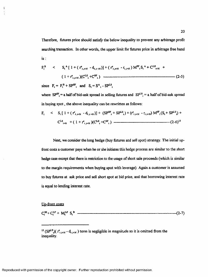
20
Therefore, futures price should satisfy the below inequality to prevent any arbitrage profit
searching transaction. In other words, the upper limit for futures price in arbitrage free band
i s :
F,B < StA [ 1 + ( r*t>t+N - d^* ,)] + ( r*t>t+N - rt t+N) MSFtStA + C“ hN +
( I + i' . jhnX ^ + C * , ) -------------------------------------------------------- (2-5)
since F, = FtB + SPSFt and St = SAt - SP“ t
where SPSF[ = a half of bid-ask spread in selling futures and SP^, = a half of bid-ask spread
in buying spot, the above inequality can be rewritten as follows:
F, < S, [ 1 + ( i*. j * - d ,,.„ )] + (SP®, + SP15,) + - r , , ^ M ", (S.+ SP^J +
C " * + ( 1 + XC“ , +Csl'l ) ------------------------------------------- (2-6)ls
Next, we consider the long hedge (buy futures and sell spot) strategy. The initial up
front costs a customer pays when he or she initiates this hedge process are similar to the short
hedge case except that there is restriction to the usage of short sale proceeds (which is similar
to the margin requirements when buying spot with leverage). Again a customer is assumed
to buy futures at ask price and sell short spot at bid price, and that borrowing interest rate
is equal to lending interest rate.
Up-front costs
Ctss+C,LF+ StB ---------------------------------------------------------------------------- (2-7)
15 (SP^tX r6, t+N - d, l+N ) term is negligible in magnitude so it is omitted from the inequality.
Reproduced with permission of the copyright owner. Further reproduction prohibited without permission.

r
21
where StB = bid price of spot index at time t (initiation)
C,55 = brokerage commissions for selling short spot
C ^ = brokerage commissions for buying futures
Mtu?= initial margin requirement ( as % of spot index ) for buying futures
At expiration date ( T= t + N ), two positions are closed by reverse transactions and the
subsequent cashflows are as follows:
Cash flows from futures
-F,A + St+N + ( 1 + r, t+N ) StB ---------------------------------------------------------- (2-8)
where F,A = ask price of futures at time t ( contract price at initiation)
Cash flows from spot
Suppose an arbitrageur faces the restriction to using the proceeds from short-sale of
borrowed securities, i.e., there is a margin requirement upon the short-sale proceeds, then the
cash flow from spot at expiration will be :
-S,+N - d,.l+H S,B + (1 + r et ,+N)( 1- M,ss) StB + ( 1 + rt t+N ) H ss S* B - Cssl+N --(2-9)
where M,ss = margin requirement ( as % of spot index ) for proceeds from short sale
Csst+N = brokerage commission for reversing short position in spot (buying spot) at
expiration
If this customer did not engage in hedge transaction, he could have used the money for up
Reproduced with permission of the copyright owner. Further reproduction prohibited without permission.

22
front costs in other interest bearing investment. Therefore, the foregone profit from other
alternative investment will be equal to :
Opportunity cost of capital for up-front costs
( l + r % N)[ Q“ + C tlF+ M ^ S ,8 ] -------------------------------------------------------- (2- 10)
Transaction for arbitrage profit is triggered if the sum of (2-8) and (2-9) exceeds (2-10).
Therefore, futures price should satisfy the below inequality to prevent any arbitrage profit
searching transaction. In other words, the lower limit for futures price in arbitrage free band
is :
FtA > StB[( l+ i V J - d ^ ] - ( r*l>t+N - r,<t+N) M1*,StB - ( r*M+N - rt,t+N) MsstSt8
- - ( 1+ rVt+N )(Csst +C“ , ) ------------------------------------------------(2-11)
since F,= FtA - SP^, and St = SBt +SPss,
where SP^, = a half of bid-ask spread in buying futures and SPss, = a half of bid-ask spread
in short-selling spot, the above inequality can be rewritten as follows :
F, > St [ (1 + r*t t+N) - d,,t+N ] - (SP^, + SPsst) - (r*til+N - r,.t+N) M ^ S , - SPS!\)
- ( - r«.*N ) ^ . ( S , - SP55,) - Csst+N - ( 1 + r ^ )(Csst +C^t ) ---- (2-12)16
i6 (.spss^ )[• j* (+N . ^ t+N ] term is negligible in magnitude so it is omitted from the inequality.
Reproduced with permission of the copyright owner. Further reproduction prohibited without permission.

23
From the above example, the arbitrage free band within which futures price fluctuates without
triggering arbitrage transaction can be suggested as such 17:
s , [ ( l + rYwJ- d.j.Ml- (SP^. + SP55,) - (tv,,* -r ,,.K)lvF,(St -SP“ )
- ( > * .« .-r,.wN)Mss,(Sl -SPss,) -C ss,.N - ( l + i * I.„N)(Css,+Cu’,) * F, £
S, [( 1 + r“,w ) - <t.,.N ] + (SP"i + SP“, ) + - <,.») Msi;($ + SPLi ) +
Cu,.„ + ( 1 + 1*,.,.* XCU, +CSF, ) ---------------------------------------------------------(2-13)
In Korea, stock index arbitrage is expected to be mostly undertaken by floor members
and other institutional investors18, and these institutional investors are assumed to be “quasi
arbitrageurs” who already own shares and sufficient funds to carry out arbitrage transactions.
They are unlikely subject to either the margin requirements in leveraged buying or shortsale
17 Suppose r*t t+N is equal to r, t+N, then the arbitrage free band would be simplified such as:
S, [(1 + r®, l+N) - d , ,^ ] - (SP1* + SPsst) - Csst+N - ( 1 + r®M+N )(Csst 4C * ) s F, s
S, [( 1 + r W - d,,t+N ] + (SPSF, + SP1*,) + C ^ t+N + ( 1 + r*t ,+N XC“ +CSFt )
18 There are 48 floor members in Korea stock exchange (KSE), all of which are securities companies licensed by Ministry of Finance (MOF). Among them, 42 securities firms including 33 domestic firms and 9 foreign branches are allowed to participate either in dealing and brokerage of stock index futures while the rest 6 can only do brokerage businesses. Other institutional investors are banks, insurance companies, investment trust companies and merchant banks. KSE sets the minimum initial margin for entry in stock index futures transaction at Won 30 million in cash (about US $ 36,000) to discourage small individual investors’ market participation.
Reproduced with permission of the copyright owner. Further reproduction prohibited without permission.

24
restrictions.19 Therefore, for these institutional investors, Iffj = 1, = .05 (zero for
member), = 0 and = .05 (zero for member) and the arbitrage free transaction band
becomes simplified as follows:20
St [ (1 + rVt+N) - d,,t+N ] - (SP^, + SP53,) - .05(1-%^ - r,,+N)(St - SPsst) - Csst+N
- (1 + rV,+N )(Csst +C^t ) s Ft ^ St [(1 + f't.t+N ) - d,>t+N ] + (SPSFt + SP^t) +
■05(r*tt+N - rl H.NXSt+ SP^d + C ^t+N + ( 1 + XC“ t +CSFt ) ----------------------- (2-14)
If we express the brokerage commissions and bid-ask spread as a percent of spot index and
turn unannualized market interest rates and dividend yields into continuous compounding, the
inequality equation (2-13) can be rewritten as follows :
19 For individual investors, the margin requirements in leveraged buying (M,1 ) is 40% and that for net proceeds from short sale (M,^) is 100%. Margin loans or securities lending for shortsale to an individual customer are provided by either Korea Securities Finance Corp. (KSFC) or brokers themselves. However, short-selling is less common practice in Korea, accounting for mere .09% of total market turnover on the KSE. Proceeds from short sales o f borrowed stocks are normally deposited at broker’s house as a collateral. There exist many restrictions regarding short-selling such as maximum amount (Won 50 million per customer and 10% of total shares of a eligible company), eligible share (the 1st section and with paid in capital in excess of Won 1 billion), etc.For institutional investors, from September 1 of 1996, securities lending system is introduced by Korea Securities Depository (KSD) as an intermediary connecting stock lenders and borrowers. Borrowing commission was set at 1.8% per annum.
20 Since KSE allows its members to use fully marketable securities they hold as substitutes for margin requirements and other institutional investors also can use them up to 10%, only 5% cash requirement for margin will be applied to the arbitrage free condition.
Reproduced with permission of the copyright owner. Further reproduction prohibited without permission.

I
where
25
S, I 1 - ATjs - lexp’®'-'” 6® - £ DlrJe x < Fr <7=1
St [ 1 + Jexp^7* ^ 6 - £ D 'jxp /V -t'r t365* (2-15)7=1
S, = current spot value
F, = current futures value
Kss = transaction costs ( as % of spot index value) of being short in the spot
including brokerage commissions, bid-ask spreads and foregone interests
on restricted short sale proceeds
Ku = transaction costs ( as % of spot index value ) of being long in the futures
including brokerage commissions, bid-ask spreads and foregone interests
on initial margin requirement
= transaction costs ( as % of spot index value ) of being long in the spot
including brokerage commissions and bid-ask spreads
Ksf = transaction costs ( as % of spot index value) of being short in the futures
including brokerage commissions, bid-ask spreads and foregone interests
on initial margin requirement
r = effective market interest rate per annum
t = current ( initiation )date
T = expiration date
£ Dt+j expr<T'(,+iV36S) (j=l,2,....,T-t) = future value of dividends on spot between t
and T at expiration (time T)
Reproduced with permission of the copyright owner. Further reproduction prohibited without permission.

26
2-2-4. Measures of Futures Mispricing
In the previous literatures, the deviation of the actual futures price from theoretical
price is usually expressed as percentage of spot index value such as below:
M, = (Ft - F*) / St x 1 0 0 -------------------------------- (2-16)
where F* = theoretical futures price based on the cost of carry model
When transaction costs are taken into account, the mispricing of futures can be defined by the
deviation from the arbitrage free band :
M, = (F, - F ) / F x 100 If Ft > F
= 0 If F * Ft * F
= (F, - F ) / F x 100 If Ft < F ---------------- (2-17)
where F = upper bound futures price in arbitrage free band
F = lower bound futures price in arbitrage free band
Suppose once established arbitrage position is held to the expiration date21, the annualized
expected excess arbitrage return to expiration (AERE) can be calculated.This has an identical
21 Brennan and Schwartz (1990) argue that opening a futures position carries with it an option to close out early and thereby make an additional arbitrage profit. Sofianos (1993) suggests that an arbitrageur may initiate arbitrage position even if fixtures mispricing does not fully cover transaction costs because of this profitable early exercise option. Early closing of position becomes valuable whenever profitable mispricing reversal occurs so that futures contract switches from being overpriced by an amount exceeding transaction costs to being underpriced by an amount exceeding transaction costs. Sofianos insists that the arbitrageur needs smaller mispricing to close a position profitably (early) than to open the position due to lower transaction costs involved. He also documents that more than 70% of futures positions are unwound before the expiration in practice.
Reproduced with permission of the copyright owner. Further reproduction prohibited without permission.

27
implication to the return on investment (ROI) in the capital budgeting decision making.
Annualized expected excess arbitrage return to expiration fAERF)
(i). At short hedge ( long in spot and short in futures )
(365/ number of days to expiration)/ [ ( actual futures price - upper bound)/ arbitrage capital)]
( 365/N )[ (Ft - F ) / [ S,A + C “ + CtSF + H SF St A ] --------------------------- (2-18)
where F* = upper bound futures price in arbitrage free band
N= time to expiration (T-t)
(ii). At long hedge ( short in spot and long in futures )
(365/ number of days to expiration)/ [( lower bound - actual futures price )/ arbitrage capital)]
(365/N )[ (F, - Fty [ StB + C,58 + C ” + M ,^ StB ] ---------------------------(2- 19)
where F = lower bound futures price in arbitrage free band
In addition to checking the frequency and magnitude of the mispricing (deviations
from arbitrage free band), implied repo rate (IRR) may be compared to the market interest
rates to see how often futures price moves outside the arbitrage free band, i.e., profitable
arbitrage opportunities are created. This procedure is introduced by Brenner, Subrahmanyam
and Uno (1989,1990). Implied repo rates (IRR) is similar to the internal rate of return (IRR)
in capital expenditure decision making and equalize the actual futures price with theoretical
price when applied to the given current spot price, maturity, and dividend streams.
Reproduced with permission of the copyright owner. Further reproduction prohibited without permission.

28
REPO, = ( 365/ N )[ In {F, /[ S, - PV( Div,)]}]--------------------------- (2-20)
where PV( Div, ) = present value of dividends paid on spot between t and T
N= time to expiration (T -t)
When transaction costs are considered, implied repo rate (IRR) can be modified such as :
Implied repo rates (IRR) under transaction cost consideration
(I)REPO, = (365 /N )[ln{F ,/[S , ( l - K ss-K LF)-PV (D iv,)]}] if F, < F , (2-21)
In this condition, REPO, < r and an arbitrageur can make excess return by short selling spot,
lend the proceeds at market rates and buying futures to lock in a lower borrowing rates.
(ii) REPO, = r if F, < F, < F , --------------------------------------------------- (2-22)
In this condition, no arbitrage excess return ( out of risk free return) can be made.
(iii)REPO, = ( 365/ N )[ In (F, /[ S, ( 1+ Kss + ) - PV( Div,)]}] if F, > F , (2-23)
In this condition, REPO, > r and it becomes profitable to borrow funds at market interest
rates, buy spot, and sell futures to lock in a higher lending rates.
2-3. Empirical Studies Regarding the Mispricing of the Futures Contracts
2-3-1. Corporate Practice of Dividend Payments in Korea
Before we investigate the mispricing of futures contract based upon the theoretical
Reproduced with permission of the copyright owner. Further reproduction prohibited without permission.

29
relationship between spot and futures in formula (2-15), the Korean corporate practice
regarding dividend payments first has to be considered. Above all, the dividend yield is on
average very low when compared to the other countries. According to the KSE, the market
weighted average dividend yield in 1995 was mere 1.1%. This figure is comparatively lower
than 3- 4 % in the U.S. or 4-5% in the U.K. (see Kim and Yoon 1992). Unlike the cases of
the U.S. corporations paying dividends quarterly or Japanese companies with semi annual
dividend payments, all Korean companies pay dividends once a year and their ex-dividend
dates fall exactly at the end of their fiscal years, which is the last day of any of March, June,
September or December. Since among 200 companies included in KOSPI 200 index, 175
firms (87.5%) predominantly have their ex-dividend dates in December, with only 14 firms
in March, 6 firms in June and 4 firms in September.22 Table 2-2 lists the dividend yields of
each component stock based on the dividend record in 1995. Even the largest 200
companies’ average dividend yields do not exceed 2%. Moreover, about 20% (41 firms) out
of the KOSPI component firms do not pay out at all. Since there are only ten firms (5.0%)
whose ex-dividend dates lie within our sample periods and the actual payments of dividends
normally take at least three months after ex-dividend dates, the effect of dividends stream is
presumed to be minimal and thus the effect of dividend payments on the futures pricing is not
considered in our study.23
22 There is only one firm which have its fiscal year end in January in the KOSPI 200. However, this is very exceptional case in Korea.
23 The percentage of these ten firms in total market capitalization of KOSPI 200 firms is very low (about 1.2%). Moreover, the percentage these ten firms accounts for in the weighted average dividend yields of the total KOSPI 200 index constituents is only0.56%. This means that dividends payments affect spot index only by .0163 index point
Reproduced with permission of the copyright owner. Further reproduction prohibited without permission.

iI
30
2-3-2. Estimation of Transaction Costs in Arbitrage Trading
In consideration of transaction costs entailed in the arbitrage between spot and futures
market, Table 2-3 provides transaction cost estimates for each market participant according
to their position as an investor. KSE members, who are all securities firms, have seats in the
trading floor in the KSE and perform as dealers or brokers providing liquidity in the both
stock and futures markets. Transaction costs, especially in terms of brokerage commissions,
are at minimal level for the KSE members.24 For other institutional investors such as banks,
insurance companies and investment trust companies (similar to the mutual funds in the U.S.),
transaction fees normally depend on the arrangement between the investors and the executing
members. Although it is reasonable to assume that transaction fees are higher for these types
of institutional investors than for KSE members, the difference in transaction costs between
members and institutional investors is not expected to be large due to the negotiation power
of the institutional investors and fierce competition among member firms. For individual
investors, arbitrage transaction is hardly expected since it is almost impossible for an
individual to track even a small portion of the component stocks due to the limits in available
capital, not to mention relatively high transaction fees involved. In addition, they can hardly
when we assume spot index being 100 point. According to KSE, the average annual dividend yield of Korean firms in 1995 is mere 1.1% and even that for larger firms (whose paid in capitals are above Won 75 billion and likely to be constituents of KOSPI 200 index) is 1.1%. Although this figure is relatively negligible compared to market interest rates, applying this average annual dividend yield to the calculation of theoretical futures price [ F, = S, exp('vd)(fr'‘y36S1, d= annual dividend yield] would result in underestimation of the fair futures price in our sample.
24 Sofianos (1993) reports that member firms typically pay no commission fees for proprietary index arbitrage transaction.
Reproduced with permission of the copyright owner. Further reproduction prohibited without permission.
ii
31
participate in long hedge (sell short spot and buy futures) transaction because short sales of
borrowed stocks are still not commonly practiced in the Korean stock market. At most, they
would participate in outright transaction in futures market in search o f speculative profit. In
the following study, we rule out the cases of individual investors’ arbitrages and consider
only the arbitrage opportunities facing the institutional investors including member firms. For
KSE members, 1% of KOSPI 200 index value is assumed for transaction costs incurred in the
arbitrage trading. For other institutional investors, 2% of spot index value is assigned for
transaction fees in the arbitrage transactions. Since the more efficient a market is operating,
the less trading costs are incurred, these figures are, on average, set at higher level than those
of the comparable markets in other countries such as the U.S. and Japan.
2-3-3. Study on the Mispricing of Futures
In Table 2-4, deviations of actual futures price from the theoretical level are illustrated
as percentage of KOSPI 200 index. In most cases during our sample period, actual futures
price deviates below the theoretical level. This is consistent with previous studies
documenting significant underpricing of futures in early introduction periods.25 In particular,
the absolute mispricing in terms of median increases monotonically with the time passage. For
December contract, all deviations take on negative value. Over the sample period, the stock
market condition in Korea has been depressed due to deteriorating economic fundamentals
25 The magnitude and frequency of mispricing of futures contract in Korean market are comparable to those observed in the Japanese market in its early inception period.Brenner, Subrahmanyam and Uno (1989) document that during 1986.12-1988.6, the percentage of negative mispricing is 73% with mean positive deviation (.51%), mean negative deviation (-1.39%) and mean absolute deviation (1.15%).
Reproduced with permission of the copyright owner. Further reproduction prohibited without permission.

32
such as slower economic growth and ballooning trade deficit. KOSPI index fell by 13.5% and
KOSPI 200 index tumbled by 19.3% during the sample period. This indicates that larger
firms suffered more under unfavorable market conditions. When we consider that the KOSPI
and KOSPI 200 rose back by 10.47% and 10.35% during December contract period (from
September 13 to October 16) due to 2% increase in foreign share ownership on October 2nd,
the market downturn during the June and September futures contract periods was very
serious (KOSPI and KOSPI 200 dropped by 9.42% and 11.80% during June contract period
and additionally fell by 8.82% and by 11.59% over September contract period). This result
is also consistent with Figlewski (1984a) in that underpricing of futures contract is more
severe when the market runs on the downside.
Chart 2-1 shows the trend of mispricing series of futures contracts graphically. Futures
price relatively hovers around the theoretical value during the June contract period. During
September contract period, the mispricing series fluctuate wildly and the standard deviation
(2.0%) is the highest. It is noticeable that futures mispricing is the most severe around the
expiration dates. Our sample covers only two expiration dates (June 13 and September 12)
and a few days before these two maturity dates, futures price drops sharply below its
theoretical level. This indicates either that investors sell heavily futures contract in search of
speculative profit or that investors who had originally long positions in futures reverse their
positions to reduce capital loss as maturity approaches.
Table 2-5 shows the autocorrelation and partial autocorrelation coefficients of the
mispricing series. As the previous empirical studies have documented (e.g., see MacKinlay
and Ramaswamy 1988 ; Yadav and Pope 1990 etc.), mispricing series shows severe positive
Reproduced with permission of the copyright owner. Further reproduction prohibited without permission.

33
1st order autocorrelation. Since partial autocorrelation function drops off after lag one, the
mispricing series can be approximated by AR(1) process. According to Garbade and Silber
(1983), the value of the first order autocorrelation coefficient represents an inverse measure
of the elasticity of supply of arbitrage services. Therefore, the smaller the value of the first
order autocorrelation coefficient, the more quickly futures price converges back to its
respective theoretical price by the arbitrage forces once it deviates from the cost of carry
relationship. The value of first order autocorrelation coefficient reveals that the inflow of
arbitrage capital is not sufficient in the early inception period. The autocorrelation coefficient
of first differenced mispricing series (Yadav and Pope (1990) call it mispricing returns)
represents degree of mispricing reversal. If past futures price is underpriced, arbitrage forces
push futures price to rise and it normally causes a negative autocorrelation between
successive price changes. The autocorrelation of first differenced mispricing also supports the
lack of arbitrage activities by market participants in the Korean market. Except for December
contract, the 1st order autocorrelation of mispricing returns is positive, not negative as
reported in other markets (the S&P 500 index futures in MacKinlay and Ramaswamy 1988
or UK FTSE 100 index futures in Yadav and Pope 1990). In Korean futures market,
mispricing seems to persist for at least over 10 minutes in the early period.
In Table 2-6, descriptive statistics of the annualized implied repo rates (IRR) are
reported and Chart 2-2 shows the trend of IRR graphically. As is shown in the Chart 2, IRR
fluctuates mostly below the 3 month CD rates (used as riskless interest rates) and especially
hovers below zero over September contract period . The negative median IRR indicates that
over the September contract period, futures price frequently fall even below spot index value.
Reproduced with permission of the copyright owner. Further reproduction prohibited without permission.

34
This fact suggests that although futures underpricing persists in the early introduction period
and gives market participants plenty of arbitrage opportunities (by selling short spot and
buying futures), the lack of arbitrage capital fails to realign futures price back to its normal
level. In its latest reports, Korean Economic Daily (KED) attributes the reason for lack of
arbitrage activities by the institutional investors to the unfavorable stock market condition.
Before the opening of the index futures market, the stock market was bullish with KOSPI and
KOSPI 200 having risen by 12.26% and 14.39% respectively from March 2nd to May 1st.
During this time period, institutional investors make errors in forecasting the future direction
of stock price and pile a host of stocks in their own account. By sudden change of market
condition from bull to bear, institutional investors would have suffered from large capital
losses if they had tried to sell short their stocks and take long position in futures as the
theoretical long hedge dictates. Because the market participation of foreign capital is
restricted, they could not fill the gap. Just like mispricing series in Chart 2-1, annualized IRR
drops sharply into negative value before expiration dates, indicating pricing anomaly is
serious near the maturity dates.
2-3-4. Analysis of Ex Post Arbitrage Profitability
Table 2-7 reports the results for test of profitability of ex post arbitrage transaction
in case that 1% transaction costs (as percentage of KOSPI 200 index) are accounted for.
Chart 2-3 also shows graphically the upper bound and lower bound of theoretical arbitrage
free band as well as actual futures price. As is seen in the Table 2-7, the frequency of
deviation from theoretical arbitrage band increases with time passage. For June contract, only
Reproduced with permission of the copyright owner. Further reproduction prohibited without permission.
35
5.5% of total observations deviate out of the arbitrage free band but for December contract
period, 97% of the total observation falls beyond the lower boundary of arbitrage free band.
Absolute deviation from theoretical band displays the asymmetry between upward mispricing
and downward mispricing. The frequency and magnitude of positive mispricing beyond the
upper boundary are only 162 case (5.6%) and .2510 compared to 1387 cases (47.6%) and
2.0117 in the negative mispricing below the lower boundary. By locking in the long hedge
(sell short spot and long futures) until maturity, an arbitrageur can gain on average 10.3%
extra annual return above the riskless return (annualized excess return to maturity: AERM)
while short arbitrageurs (sell futures and long spot) gain only 7.6% extra return in lower
chances. Figlewski (1984b) reports that during the early inception period (1982.6-9), the
nearby S&P 500 futures contract provides investors with about 6% excess return by taking
long arbitrage. Therefore, index futures underpricing in the its early inception period is on
average slightly more severe in the Korean market. Chart 2-4 displays graphically the
magnitude of mispricing over the sample period after accounting for 1% transaction costs.
In Table 2-8 and Chart 2-5 extend the transaction cost to 2% of the KOSPI 200 index
value. The 2% transaction costs eventually eliminate the arbitrage opportunity by short hedge
(long spot and short futures) and reduce the frequency of mispricing from 48% to 34% of the
total observation. Moreover, investors end up without arbitrage opportunities in the June
contract period. However, in September contract period, the percentage of futures
underpricing is reduced only by 7% with large unexploited arbitrage opportunities. Over total
contract periods, an arbitrageur can still reap 9% above the CD rates annually by taking long
arbitrage transaction. Would there be any chances of early exercising to capture extra risk
Reproduced with permission of the copyright owner. Further reproduction prohibited without permission.

36
free returns? The answer is Yes for KSE members. When 1% transaction costs are accounted
for, futures price falls off below the lower boundary of arbitrage free band from June 14 th
through June 26 th, and then rises above the upper boundary of arbitrage free boundary from
August 21 to September 3rd. If a member had launched a long futures-short spot arbitrage
at the end of June and closed that position by reverse transaction at the end of August or the
beginning of September, it would have doubled its arbitrage returns relative to holding its
position up to maturity. Chart 2-6 shows graphically the mispricing of futures contract over
the sample period when 2% transaction costs are taken into account.
2-3-5. Analysis of Ex Ante Arbitrage Profitability
In addition to the ex post analysis of arbitrage opportunity, the ex ante analysis
(similar to the one proposed by Chung 1991) regarding futures mispricing is also investigated.
Ex post analysis is based on the assumption that a program trader can establish an arbitrage
position at the prices prevailing when the hedge is initially identified as profitable. However,
if prices are corrected promptly, it may not be profitable ex ante for a program trader to
construct the short or long hedge that are identified as profitable ex post. Then arbitrageurs
are exposed to substantial execution risk. On the other hand, execution prices may actually
be better than the quoted prices (observed price ex post) if mispricing in the market persists
for some reason. In the Korean stock and futures markets where only limit orders are
currently allowed, only risk incurred in order execution is that arbitrageurs’ orders remain
Reproduced with permission of the copyright owner. Further reproduction prohibited without permission.

37
unfilled at the desired bid or ask price that can be different from quoted market price.26
Therefore, execution risk is minimal in the Korean market when compared to the U.S. where
market orders prevail. As a result, the ex ante analysis in the Korean market measures how
quickly profitable mispricing opportunities disappear and tests an operational or informational
efficiency of the Korean capital market. Since our data covers intraday price data over a 10
minute interval, our ex ante analysis examines the frequency and magnitude of possible
arbitrage profits when an arbitrageur observes the futures mispricing at time t and executes
an order at time t+1 price, i.e., at price available 10 minutes later in search of ex post
arbitrage opportunity. Chung (1991) documents that when 1% transaction costs and 5 minute
execution delay are accounted for, almost half of ex post arbitrage opportunities become
unprofitable at ex ante basis. Klemkosky and Lee (1991), however, report that the arbitrage
position is still profitable even 10 minutes after it is initially identified as profitable. In
analysis of ex ante arbitrage profitability, we consider two different cases regarding execution
lag in the practice. First, we can assume that an arbitrageur can sell or buy futures as soon
as mispricing opportunities are observed, but 10 minute later in spot market. Alternatively,
we can also assume that an arbitrageur takes action quickly in spot market as soon as he or
she notices mispricing but 10 minute later in futures market. While it is reasonable to assume
execution lag in both markets (Chung 1991), spot trading involves simultaneous trading of
component stocks in the basket (even though development o f program trading substantially
reduces execution lag) and thus, the former case can be more close to reality than the latter
26 Market orders are introduced in the Korean Market on November 25,1996, which is outside of the sample period of this study.
Reproduced with permission of the copyright owner. Further reproduction prohibited without permission.

38
case. Sofianos (1993), however, mentions legging (the cash and futures position in an
arbitrage transaction are not established or liquidated simultaneously) in which case an
arbitrageur can deliberately submit orders earlier or later in futures market than in cash market
in search of bigger arbitrage profit.27 Therefore, results under two different scenario are
presented in our analysis. Table 2-9 and Table 2-10 display results o f the ex ante arbitrage
profitability in case of 1% and 2% transaction fees incurred respectively when there is 10
minute execution lag in spot trading. Consistent with Klemkosky and Lee’s study (1991),
only 59 cases (2.0%) out of total ex post mispricing for 1% transaction costs and 24 cases
(0.7%) cases for 2% transaction costs become unprofitable ex ante. In terms of median
annualized access return to maturity (AERM), the ex ante profit (10.30% from underpricing
and 6.54% from overpricing for 1% transaction costs, and 8.16% from underpricing for 2%
transaction costs) turns out to be greater than corresponding ex post profit (9.36% and
6.07% for 1% transaction costs and 7.94% for 2% transaction costs). This indicates that
mispricing is not corrected within a 10 minute interval, but tend to persist in the same
direction. Although standard deviation of ex ante profitability (AERM) is slightly higher
(i.e., the arbitrage is more risky ex ante) than that of ex post profitability in case of 1%
transaction costs, the opposite is true when 2% transaction costs are accounted for. Table 2-
11 and Table 2-12 show results of the ex ante arbitrage profitability in case of 1% and 2%
27 Sofianos takes an example of legging as such : “suppose the futures price drops ahead of the cash price, so that the cash market is overvalued. The arbitrageur should buy the futures and sell the cash. The arbitrageur, however, expects the futures price to continue falling before the cash starts falling and sell the cash immediately but delays buying the futures until they are cheaper. If the arbitrageur’s expectations are confirmed, delaying the futures side of the transaction locks in a bigger mispricing ” (see Sofianos (1993), p.p. 16).
Reproduced with permission of the copyright owner. Further reproduction prohibited without permission.

39
transaction fees incurred respectively when there is 10 minute execution lag in futures trading.
Again, only 54 cases (1.9%) of 1% transaction costs and 32 cases (1.1%) of 2% transaction
costs become unprofitable at ex ante basis. Since underpricing of futures contract tends to
be persistent over the sample period, it is not unreasonable to observe that mispricing is not
eliminated as quickly as the efficient market dictates. This also supports MacKinlay and
Ramaswamy’s (1988) path dependence hypothesis of futures mispricing, which states that
once futures price crosses either upper or lower bound, it takes a while for such mispricing
to touch the other side of the boundary.
2-3-6. Relationship of Futures Mispricing with Time to Expiration
Our study also examines the Cornell and French’s (1983) tax timing option hypothesis
or Brennan and Schwartz’s (1990) early closing option hypothesis regarding the futures
pricing. Although these two hypotheses suggest different explanations for futures
underpricing below the theoretical level, they both expect futures’ underpricing to decrease
as the expiration date approaches. In panel 1 of Table 2-13, all mispricings have significant
negative relationships with the time left to maturity, which is consistent with either tax timing
option hypothesis or early exercise option hypothesis. We also investigate MacKinlay and
Ramaswamy’s (1988) argument that the absolute mispricing is positively related to the time
left until maturity in panel 2 of Table 2-11. Indeed, this regression suggests that the
magnitude of mispricing continues to shrink as the maturity approaches. In the panel 3 of
Table 2-11, we regress the futures mispricing on the return on stock market to see if the
market condition can account for, at least partially, the severity of futures underpricing over
Reproduced with permission of the copyright owner. Further reproduction prohibited without permission.

40
the sample period. Consistent with Figlewski (1984a), the more the stock market falls, the
more severe the underpricing of the futures contract is, especially over September and
December contract periods.2*
2-3-7. Basis and Arbitrage Trading
Table 2-14 provides the descriptive statistics and autocorrelation coefficient of the
basis and Chart 2-7 displays the trend of basis graphically. As shown in the previous analysis,
the futures price frequently falls below the corresponding spot price, resulting in negative
basis over September contract period. Negative autocorrelation in the basis changes are said
to result from active arbitrage forces in the market. Miller, Muthuswamy and Whaley (1994),
however, insist that the negative autocorrelation in basis changes may result from statistical
illusion, i.e., the positive first order autocorrelation in spot index changes due to infrequent
trading. Even without any significant arbitrage forces involved, asynchronous trading effect,
i.e., positive autocorrelation in spot index may spuriously induce basis change to have
negative serial correlation. In our sample, except for December contract, the basis changes
take on positive first order autocorrelation, not a negative one as in other studies. This is
mainly due to the fact that unlike studies regarding futures market in the U.S., the changes
of futures price have the significant positive first order autocorrelation rather than negative
first order autocorrelation if any. This fact also may confirm the persistence of futures
underpricing and lack of arbitrage forces. Dwyer Jr., Locke and Yu (1996) report that in
2* Over June contract period where futures price moves closely with theoretical value, stock market movement does not explain changes in mispricing.
Reproduced with permission of the copyright owner. Further reproduction prohibited without permission.

ii
41
response to positive or negative shocks to the cash index, the basis returns to values inside
the transaction cost bounds only after more than 20 minutes. They also document that the
basis converges faster to the normal when arbitrage is profitable than when arbitrage is
unprofitable. Harris, Sofianos and Shapiro (1994) similarly document that it takes an average
of 10 minutes after a program trade for the basis to revert to a theoretically correct value.
They also find that the basis returns to the normal level more quickly for buy rather than sell
(spot) index arbitrage trades. Our result is generally consistent with their findings in that the
basis tends to be corrected only after more than 10 minutes, and in that persistence in basis
(mispricing of futures price) results mainly from inactive arbitrage trades that are in turn
caused by unfavorable spot market condition.
Finally Table 2-13 summarizes the actual trading activities during our sample periods.
Consistent with our previous analysis, the arbitrage transactions have shrunken substantially
in both number and amount since June contract, leaving persistent arbitrage opportunities
unexploited. While the level of trading volume and open interest relatively remain stable
during the whole sample periods, the percentage of arbitrage trading to the total trading
decreases continuously from 1.4% in June to 0.6% in July, 0.4% in August, 0.2% in
September and 0.3% in December. This fact confirms inactive arbitrage transactions in the
Korean futures market in the early introduction period.
2-4. Conclusion
In this chapter, we analyze the mispricing of futures contract in the early inception
period. Our analysis takes into account transaction costs incurred in index arbitrages that are
Reproduced with permission of the copyright owner. Further reproduction prohibited without permission.

42
executed mainly by institutional investors and KSE members. Consistent with previous
empirical studies concerning the pricing of index futures in other countries, futures contract
in the Korean market have been undervalued relative to the theoretical price based upon the
cost of carry relationship. When 2% transaction fees (relative to spot index value) are
considered, however, futures price of June contract moved within the boundary of arbitrage
free band. Futures contract began to deviate substantially from its fair value and sometimes
even below its corresponding cash value since June and left plenty of long arbitrage
opportunities (sell short spot and long futures). However, most of these arbitrage
opportunities have not been exploited by the investors so that the trend of futures
underpricing persists. Bearish stock market condition seems to have resulted in substantial
capital losses on the existing stock portfolio of institutional investors and this may have made
them unable to capture these profit opportunities by taking long hedge. Even after accounting
for 10 minute execution lag, most of arbitrage profit opportunities are still left unexploited
and long futures-short spot arbitrage would have resulted in substantial extra returns above
the riskless rates even on the ex ante basis.
Several reasons for futures mispricing can be raised. First, lack of arbitrage capital due
to market regulations (for example, withdrawing of gains from marking to market is
prohibited) or limited participation o f experienced foreign capital could have caused the
underpricing. Second, as Figlewski (1984b) notes, the market inertia caused by the
practitioner’s unfamiliarity would be a reason for underpricing.
Reproduced with permission of the copyright owner. Further reproduction prohibited without permission.

Table 2-1. Main Features of Korean Stock Index Futures Contract
1. Underlying asset
2. Contract size
3. Contract Months
4.Last day of trading preceding
5.Settlement date
6.Trading hours*
7. Method of trading
8. Tick size
9. Settlement procedure
10.Price limitsb
11 Margin'
KOSPI200Market value weighted index o f the 200 representative Stocks ( its base index point is 100 as of Jan3,1990)
KOSPI 200 multiplied by Won 500,000 (about US $600)
March, June, September and December ( Four contract months open at a time so that longest maturity period is one year)
The second Thursday of the delivery month or the day
the second Thursday in case the second Thursday is a holiday
The second business day after the last trading day
Ordinary davWeekday : 9:30 - 11:30 a.m. ( morning session)
1:00 - 3:15 p.m. ( afternoon session)Saturday : 9:30 - 11:45 a.m. ( morning session only )
Last trading dayWeekday : 9:30 - 11:30 a.m. ( morning session)
1:00 - 2:50 p.m. ( afternoon session)Saturday : 9:30 - 11:20 a.m. ( morning session only)
Computer assisted auction
0.05 index point that is equivalent of Won 25,000 ( 0.05 x Won 500,000 )
Cash settlement
±5% of the previous settlement (closing) price
KSE Members ( Securities firms 1 10 % of transaction value
Customers D Initial margin15% of transaction value ( at least 5% cash)
Reproduced with permission of the copyright owner. Further reproduction prohibited without permission.
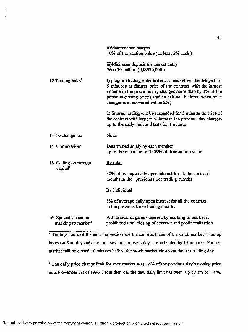
Ii
44
ii)Maintenance margin10% of transaction value ( at least 5% cash )
iii)Minimum deposit for market entry Won 30 million ( US$36,000 )
12.Trading haltsd I) program trading order in the cash market will be delayed forS minutes as futures price of the contract with the largest volume in the previous day changes more than by 3% of the previous closing price ( trading halt will be lifted when price changes are recovered within 2%)
ii) futures trading will be suspended for 5 minutes as price of the contract with largest volume in the previous day changes up to the daily limit and lasts for 1 minute
13. Exchange tax
14. Commission'
15. Ceiling on foreign capitaf
16. Special clause on marking to market®
None
Determined solely by each memberup to the maximum of 0.09% of transaction value
By total
30% of average daily open interest for all the contract months in the previous three trading months
By Individual
5% of average daily open interest for all the contract in the previous three trading months
Withdrawal of gains occurred by marking to market is prohibited until closing of contract and profit realization
1 Trading hours of the morning session are the same as those of the stock market. Trading
hours on Saturday and afternoon sessions on weekdays are extended by 15 minutes. Futures
market will be closed 10 minutes before the stock market closes on the last trading day.
b The daily price change limit for spot market was ±6% of the previous day’s closing price
until November 1st of 1996. From then on, the new daily limit has been up by 2% to ± 8%.
Reproduced with permission of the copyright owner. Further reproduction prohibited without permission.

45
c Margin requirement is stricter in Korean market relative to the U.S. In the U.S., the margin
requirement differs according to the type of transaction and varies from time to time. For
example, CME requires US$16,800 per contract as initial margin and US$ 15,000 per
contract as maintenance margin for speculative trading as of 1997. In contrast, both initial
and maintenance margin for member’s proprietary arbitrage trading are US$8,000 per
contract and those for intramarket spread trading are only $169 and $150 per contract
respectively. Therefore, the initial and maintenance margin for customers set by member’s
discretion are no greater than 5% even for speculative trading in case of S&P 500 futures.
On the other hand, in Japanese TOPIX futures (as o f 1997), the initial margin is set at 15%
of the contract value or ¥ 6 million, whichever is greater, and the maintenance margin is set
at 12% of the contract value. At least 3% of the margin should be deposited in cash. When
margin requirements in the Korean market is compared to those set by other markets in the
early introduction period, however, the current margin level in the Korean futures market is
relatively set high to prevent default on performance and discourage small individual
investors’ market participation. In 1983, the initial and maintenance margins for speculative
trading were US$ 6,000 and US$2,500 per contract (about 9% and 4% of the contract value)
respectively in the S&P 500 futures contract. As for TOPIX futures contract, the initial and
maintenance margins were 9% and 6% of the total contract value in 1988. Members should
deposit at KSE the required margins amounting to 10% of total contract values including
their proprietary as well as their customers’ positions. For KSE members, the entire amount
of margin may be deposited by marketable securities unlike customers. Also, KSE members’
margin will be computed based on the first futures price of a contract and this base price will
not be changed until the futures price changes by more than 30%. The leverage effect of
futures over spot trading in the Korean market is relatively low compared to the case in the
U.S. market. In the U.S., Federal Reserve Board (FRB) requires at least 50% of margin in
spot trading while 40% of margin is required in Korean spot market. Therefore, the leverage
effect of futures is about 2.7 times greater than that of spot trading in Korea while in the
U.S., futures’ leverage effect is about 10 times greater than that of spot trading.
d In case of I), there will be no trading halt 30 minutes before closing of daily trading.
Reproduced with permission of the copyright owner. Further reproduction prohibited without permission.

46
In case of ii), if there has been a trading halt in a day, there will be no more trading halts in
the same day. Also, there will be no trading halt after 2:20 p.m. (10:50 a.m. in the absence of
afternoon session).
e Official commission rates set by some members as follows :
Daewoo Securities C o .: Transaction value < Won 500 mil.
< Won 1 bil.
< Won 5 bil.
> Won 5bil
Dongsuh Securities Co. : Transaction value > Won 5bil
0.05%
0.045% + Won25,000
0.040% + Won75,000
0.035% + Won325,000
0 .020%
The other ranges are same as Daewoo Securities Co.
Dongwon Securities C o .: Transaction value < Won 1 bil. : 0.03%< Won 2.5 bil. : 0.02% + Won50,000 > Won 2.5 bil : .020% + Wonl75,000
However, large customers like institutional investors tend to negotiate commission rates with
members and pay less than the above rates. (Source : Korea Economic Daily)
f From November 1 of 1996, MOF increased the ceiling on the foreign capital in index futures
from 15 % to 30% in total and from 3.0% to 5.0% per individual.
g Applying gains from daily marking to market toward the margin for other trading is also
prohibited. However, loss from daily marking to market is reflected in calculation of margin
requirement for another transactions. These asymmetric treatments for gains and losses from
marking to market process over-emphasize the riskiness of futures trading and eventually
reduces attractiveness of futures trading and efficiency of the futures market.
Reproduced with permission of the copyright owner. Further reproduction prohibited without permission.

Table 2-2. Component Stocks in KOSPI 200 ( Won Bil.)
Company FY» Mkt Cap." Div.c Div.YieIdd( M anufacturing: 139 stocks )Dong Won Ind. 12 1,301.30 44.61 3.43%Dong Bang Corp. 12 686.30 1.99 0.29%Nong Shim 6 720.00 22.50 3.13%Cheil Foods & Chemical 12 4,893.38 10.27 0.21%Hai Tai Confectionary 6 813.25 26.73 3.29%Tong Yang Confectionary 12 851.76 21.29 2.50%Miwon 12 1,587.38 9.47 0.60%Tai Han Sugar 12 684.64 14.83 2.17%Woo Sung Feed Mill 12 685.98 15.45 2.25%Sewon Co. 12 1,077.11 9.65 0.90%Samyang Genex 6 1,168.92 11.07 0.95%Jinro 9 1,630.87 58.68 3.60%Oriental Brewery 12 892.17 0.00 0.00%Chosun Brewery 12 2,362.08 0.00 0.00%Lotte Chilsung Beverage 12 1,245.19 5.42 0.44%Ssang Bang Wool 12 1,102.75 16.50 1.50%Tae Chang 1 1,040.40 8.70 0.84%Choong Nam Spinning 12 1,175.80 0.00 0.00%Dai Nong Corp. 12 923.94 12.06 1.31%Cheil Ind. 12 2,921.40 86.40 2.96%Tong Yang Nylon 12 2,160.39 44.33 2.05%Kohap 12 2,193.92 35.05 1.60%Hanil Synthetic Fiber 12 1,128.11 0.00 0.00%Kolon Ind. 12 2,215.37 12.61 0.57%Sun Kyung Ind. 12 2,398.58 58.39 2.43%Cheil Synthetic Textiles 12 1,657.60 47.46 2.86%Sam Yang 6 2,520.24 8.70 0.35%Pang Rim 9 1,549.45 9.00 0.58%Nasan Ind. 12 600.60 11.55 1.92%Shin Won Corp. 12 1,553.59 30.30 1.95%Kukje Corp. 12 1,340.23 0.00 0.00%Sung Chang Enterprise 9 1,968.00 15.00 0.76%Hankuk Paper Mfg. 12 1,095.00 26.00 2.37%Hansol Paper Co. 12 4,342.10 112.59 2.59%Shin Poong Paper 12 676.49 12.11 1.79%On Yang Pulp 6 538.84 3.90 0.72%Sepoong Corp. 12 1,029.37 0.00 0.00%Dong Hae Pulp 12 1,574.00 0.00 0.00%Ssang Yong Paper 12 764.07 17.48 2.29%
Reproduced with permission of the copyright owner. Further reproduction prohibited without permission.

!!
48
(Table 2-2 continued)Hanwha Chemical 12 5,594.39 47.73 0.85%Oriental Chemical 12 2,140.07 14.65 0.68%Korea Kumho Petro. 12 2,169.25 124.18 5.72%Isu Chemical 12 840.45 0.00 0.00%Dongbu Chemical 12 836.13 0.00 0.00%Posco Chemical 12 808.47 16.56 2.05%Han Nong Corp. 12 657.40 12.97 1.97%LG Chemical 12 12,368.46 443.68 3.59%Miwon Petro Chemical 12 898.96 3.57 0.40%Dong Sung Chemical 12 592.80 12.48 2.11%Kuk Do Chemical 12 1,145.33 30.06 2.62%Honam Petro. Chemical 12 4,651.56 238.95 5.14%Korea Chemical 12 3,120.00 40.00 1.28%Yuhan Corp. 12 1,422.72 16.23 1.14%Dong-A Pharm. 12 1,692.82 16.12 0.95%11 Yang Pharm. 12 864.16 15.77 1.82%Dong Wha Pharm 3 727.89 2.90 0.40%Choong Wae Pharm. 12 1,469.87 25.81 1.76%Chong Kun Dang 12 935.55 14.17 1.51%Korea Green Cross 12 1,779.04 13.44 0.76%Dong Shin Pharm. 12 873.15 0.81 0.09%Pacific Corp. 12 1,683.32 40.80 2.42%Hanwha Corp. 12 3,071.44 0.00 0.00%Hankook Titanium 12 768.28 26.72 3.48%Saehan Media 12 1,210.85 24.46 2.02%Yukong 12 16,687.89 362.26 2.17%Ssang Yong Oil Refining 12 12,494.63 852.66 6.82%Hanwha Energy 12 1,779.74 0.00 0.00%Han Kook Tire 12 2,116.21 32.20 1.52%Kumho 12 1,730.99 0.00 0.00%Dong-A Tire 12 1,198.88 0.00 0.00%STC Corp 12 1,205.75 33.94 2.81%Han Kook Glass 12 2,926.88 75.75 2.59%Hankuk Safety Glass 12 745.00 9.40 1.26%Hanil Cement 12 1,836.00 26.52 1.44%Asia Cement 12 1,336.00 26.00 1.95%Ssang Yong Cement 12 7,455.87 212.23 2.85%Hyundai Cement 12 1,188.00 21.60 1.82%Tong Yang Cement 12 2,703.96 82.47 3.05%Sung Shin Cement 12 1,183.49 27.72 2.34%Keum Kang 12 3,474.00 60.00 1.73%Kang Won Ind. 6 1,309.56 5.30 0.40%
Reproduced with permission of the copyright owner. Further reproduction prohibited without permission.

49
(Table 2-2 continued)Dong Kuk Steel Mill 12 4,305.60 140.40 3.26%Pohang Iron & Steel 12 47,608.21 892.06 1.87%Hanbo Steel 12 1,243.06 0.00 0.00%Korea Iron & Steel 12 1,548.00 48.00 3.10%Kia Steel 12 1,312.07 0.00 0.00%Dong Bu Steel 12 1,951.22 42.54 2.18%Sammi Steel 12 2,849.46 0.00 0.00%Inchon Iron & Steel 12 3,234.00 66.00 2.04%Hyundai Pipe 12 1,010.00 25.00 2.48%Se Ah Steel 12 1,422.91 11.20 0.79%LG Metals Corp. 12 1,560.00 48.00 3.08%Korea Zinc Co. 12 3,268.00 86.00 2.63%Poong San 12 2,974.38 86.35 2.90%Choil Aluminum 12 653.40 16.50 2.53%Dae Han Jung Suok 12 2,202.65 7.98 0.36%Daewoo Heavy Ind. 12 30,858.26 918.87 2.98%Ssang Yong Heavy Ind. 12 932.31 0.00 0.00%Hanwha Machinery 12 954.32 0.00 0.00%Kyungwon Century 3 1,596.00 45.00 2.82%Korea Computer 12 747.90 23.37 3.12%Taeil Media 12 1,675.88 35.83 2.14%Trigem Computer 12 1,666.04 34.56 2.07%Chung Ho Computer 12 2,238.97 22.02 0.98%Nae Wae Semiconductor 12 707.93 4.81 0.68%LG Electronics 12 26,803.50 311.52 1.16%Samsung Electronics 12 109,933.63 805.75 0.73%Inkel Corp. 12 569.37 15.91 2.79%Daewoo Electronics 12 6,730.67 274.07 4.07%Daeryung Ind. 12 789.83 12.41 1.57%Sungmi Telecom Electro. 12 1,689.89 24.43 1.45%Han Chang 12 1,338.52 0.00 0.00%Anam Ind. 12 2,814.96 43.65 1.55%Samsung Display Dev. 12 15,659.12 49.64 0.32%Samsung Electro-Mech. 12 8,202.05 54.46 0.66%Korea Electronics 9 1,020.21 20.00 1.96%Orion Electric 12 2,393.89 15.24 0.64%Daewoo Telecom 12 3,295.27 0.00 0.00%Dae Duk Ind. 12 419.71 1.22 0.29%Daewoo Elec. components 12 638.70 7.38 1.16%Taihan Electric Wire 12 3,528.00 100.80 2.86%LG Cable 12 2,254.50 58.18 2.58%LG Ind. System 12 5,087.69 101.75 2.00%
Reproduced with permission of the copyright owner. Further reproduction prohibited without permission.

1
50
(Table 2-2 continued)Rocket Electric 12 167.17 9.05 5.41%Kia Motors 12 13,785.19 55.88 0.41%Hyundai Motors 12 17,481.84 353.98 2.02%Ssang Yong Motors 12 3,155.01 0.00 0.00%Asia Motors 12 3,475.56 0.00 0.00%Hyundai Precision 12 3,530.53 115.47 3.27%Tongil Heavy Ind. 12 2,709.24 0.00 0.00%Mando Machinery 12 2,315.16 50.37 2.18%Yoosung Enterprise 12 735.00 14.70 2.00%Daewoo Precision 12 1,188.16 10.15 0.85%Jindo corp. 1.2 1,209.50 13.84 1.14%Hyundai Mipo Dock Yard 12 1,352.00 40.00 2.96%Samsung Heavy Ind. 12 13,078.16 321.57 2.46%Samsung Aerospace 12 4,088.00 69.40 1.70%Hyundai Wood Ind. 12 741.00 0.00 0.00%Young Chang Akki 12 900.00 11.25 1.25%( Utilities & Gas : 3 stocks)Korea Electric Power 12 189,941.94 3,083.47 1.62%Samchully 12 1,301.04 11.70 0.90%Kyungnam Energy 12 814.30 12.75 1.57%( Building & Construction : 16 stocks)Samwhan Enterprise 12 1,746.56 39.26 2.25%Dong Ah Construction 12 7,565.73 167.50 2.21%Doosan Engin. & Const. 12 1,997.25 10.84 0.54%Daelim Ind. 12 4,396.19 31.58 0.72%Sambu Construction 12 1,901.59 0.00 0.00%Hanshin Construction 12 868.03 0.00 0.00%Kuk Dong Engin. & Const. 12 1,546.00 0.00 0.00%Hanjin Engin. & Const. 12 2,631.34 0.00 0.00%LG Construction 12 2,461.30 65.20 2.65%Hyundai Construction 12 17,757.77 0.00 0.00%Kumho Const. & Engin. 12 2,975.32 34.51 1.16%Kun Young 12 1,490.58 0.00 0.00%Dong Shin Construction 12 945.00 14.00 1.48%Tai Young 12 3,082.65 33.47 1.09%Kisan 12 1,506.00 22.67 1.51%Chongu H & C 12 2,216.31 46.51 2.10%( Trades & Transport: 12 stocks )Hyundai Motor Service 12 4,646.06 90.13 1.94%Daewoo Corp. 12 10,178.69 452.38 4.44%Samsung Corp. 12 5,556.68 141.77 2.55%LG Int'l Corp. 12 3,073.17 89.31 2.91%
Reproduced with permission of the copyright owner. Further reproduction prohibited without permission.

51
(Table 2-2 continued)Sun Kyung 12 3,649.62 18.23 0.50%Shinsegae Dept. Store 12 6,240.00 8.84 0.14%Hwasung Ind. 12 1,656.80 37.33 2.25%Keumkang Dev. 12 1,904.65 44.78 2.35%Hotel Shilla 12 1,873.05 47.48 2.53%Korea Express 12 3,258.71 72.00 2.21%Hanjin Shipping 12 2,730.01 0.00 0.00%Korea Air 12 13,854.85 257.85 1.86%( Telecommunications : 2 stocks )Korea Mobile Telecom 12 33,323.97 71.65 0.22%Dacom 12 17,627.71 69.72 0.40%( Finances : 28 stocks ) Korea LT Credit Bank 12 9,610.10 219.40 2.28%Commercial Bank 12 13,175.00 255.00 1.94%Choheung Bank 12 14,809.20 328.00 2.21%Korea First Bank 12 11,316.00 0.00 0.00%Hanil Bank 12 13,744.80 332.00 2.42%Seoul Bank 12 11,037.20 0.00 0.00%Koram Bank 12 3,416.58 68.40 2.00%Shin Han Bank 12 18,626.40 616.00 3.31%Hana Bank 12 3,418.79 43.55 1.27%Boram Bank 12 2,855.12 128.88 4.51%Korea Exchange Bank 12 14,206.50 330.00 2.32%Citizens National Bank 12 11,081.89 97.21 0.88%Kyungki Bank 12 3,042.28 46.03 1.51%Daegu Bank 12 4,752.00 195.00 4.10%Pusan Bank 12 3,231.90 85.50 2.65%Kwangju Bank 12 2,646.34 88.79 3.36%Daishin Securities 3 5,155.20 0.00 0.00%Daewoo Securities 3 11,537.21 0.00 0.00%LG Securities 3 7,232.66 0.00 0.00%Hyundai Securities 3 3,168.72 0.00 0.00%Dongsuh Securities 3 5,647.07 0.00 0.00%Coryo Securities 3 3,262.01 0.00 0.00%Ssang Yong Inv. & Sec. 3 5,070.41 0.00 0.00%Dongwon Securities 3 4,476.11 53.84 1.20%Shin Young Securities 3 2,293.87 41.10 1.79%Tong Yang Securities 3 2,351.47 0.00 0.00%Samsung Securities 3 3,132.00 12.00 0.38%Hyundai M & F Insurance 3 4,058.76 44.70 1.10%Total ( Average )______________ 1,109,441.84_______17307.09_________ 1.56%* FY indicates the month to which the ex dividend date of each company belongs
Reproduced with permission of the copyright owner. Further reproduction prohibited without permission.

1
52
(Table 2-2 continued)b Market capitalization ( Won Bil.) for each company is calculated by multiplying the closing price on Dec. 31,1995 by the number of listed shares on KSE. c Dividends ( Won Bil.) include only cash outlays to shareholders, not stock dividends. d Dividend yields are computed from dividing total dividends by value of market capitalization.
Reproduced with permission of the copyright owner. Further reproduction prohibited without permission.

i
53
Table 2-3. Transaction Costs for Stock Index Arbitrage in the Korean Financial Markets, May 3rd 1996 - October I6th 1996 (As % of Spot Index Price on Basis of 90 Days Hedge Period)*_______________________________________________________
KSE Members (Securities Firms)
Other Institutional Investors
IndividualInvestors
Spot MarketfA')
1.Brokerage Commissions11 - 0.40% 0.80%
2. Transaction Tax
0.30% 0.30% 0.30%
3.Market Impact' 0.40% 0.40% 0.40%
4.Cost of Borrowing Stock for Short Salesd
- 2.20%
Futures MarketfB'l
1.Brokerage Commissions
- 0.04% 0.10%
2.Cost of Margin Requirement®
- 0.15% 0.15%
3.Market Impact 0.30% 0.30% 0.30%
Total (A+B). 1,09% 1,59% 4,25%
* Chung (1991) argues that an arbitrageur, having capital constraints and knowing the risks
of ex ante trading, may require a mispricing signal of more than the amount needed to cover
transaction costs before entering into a trade. Therefore, application of transaction costs in
Table 2-3 may overestimate the actual frequency of execution and the size of arbitrage
transactions. With regard to total transaction costs involved in arbitrages, Stoll and Whaley
(1986) report 0.6125% of spot index value and Sofianos (1993) suggests 0.2% for members
and 0.5% for institutional investors in the U.S. market. As for Japanese market, Brenner,
Subrahmanyam and Uno (1990) report 0.5% ~ 0.8% for members and 1.0% ~ 1.5% for
institutional investors. As the market matures with enhanced market depth and efficiency,
Reproduced with permission of the copyright owner. Further reproduction prohibited without permission.

54
transaction costs involved in index arbitrages should decrease. Therefore, it is natural to
expect higher transaction costs in the emerging stock market such as Korea than in the
advanced capital markets. However, Sofianos (1993) points out that transaction costs
estimated in the previous studies overstate the actual transaction costs incurred in the real
practice.
bAccording to KSE, the number of shares held by institutional investors at the end of 1995
was 32% relative to 36% for individuals. In addition, the trading proportion of institutional
investors to the total trading was 27% relative to 66% for individuals in 1995. When members
are trading stocks or futures on their account (7.2% to total stock trading value in 1995 and
9.4% in 1994), their actual costs for brokerage commission are almost nil in practice.
‘Stoll and Whaley (1986), Fleming, Ostdiek and Whaley (1996) insist that bid-ask spread is
a part of market impact costs incurred in selling and buying futures and stocks. Except for
bid-ask spread as a compensation for market makers for providing immediate order execution,
there can be a additional market impact cost in forms of a price concession for large trade.
But in our study, we only take into account the round trip bid-ask spreads as market impact
costs. As for bid and ask spread in the Korean stock market, two estimates are used in this
study since no data or study about bid -ask spreads is available. First, the tick size or the
minimum price change of a stock varies according to its price and is stratified as follows.
(Source: KSE)
The average stock price of KSE listed shares as of the end of 1995 is Won 25,021, and when
we assume that the normal trading without excessive price fluctuation is made consecutively
and continuously with bid-ask bounce by tick size, the estimated bid-ask spread is about 0.4%
Price < Won 10,000
Price < Won 100,000
Price < Won 500,000
Price > Won 500,000
Stock price Tick Size
Won 10
Won 100
Tick Size / Price (%)
< 0 .1%
< 0 . 1%
< 0 . 1%
>0.5%
Won 500
Won 1,000
Reproduced with permission of the copyright owner. Further reproduction prohibited without permission.
i
55
(Won 100/ Won 25,021).
The second method is to estimate the bid-ask spread from actual transaction data of
the representative stocks among constituent stocks in the KOSPI 200 index. Roll (1984)
argues that under an informationally efficient market, the bid-ask spread can be approximated
by 2 x (- first order serial covariance of price change)05. However, his estimation method has
two major caveats. First, the autocovariance of successive price change of a stock can be
positive so that the value of estimated spread can bear imaginary number. Second, his spread
estimates tend to be dependent upon the sample frequency or time interval. Therefore, in our
study, we employ the modified Roll’s estimation method by Hsia, Fuller and Kao (1994).
Their method removes the effect of overall market movement from observed security returns
and thereby effectively eliminates the above mentioned problems in Roll’s estimation. Details
of this modified method is as follows.
Suppose the return behavior of a security can be written as
r, = a + P r^ + et and e, takes on the first order moving average(MA) process such that
et = a, - 0 a,.! and a, is white noise with E(a,) = 0 and Cov(a, .a,^ ) =0 if k*0 or o2 if k=0.
Since Cov(rt , rM ) = P2Cov ( r ^ , r ^ ) - 0o2 and Cov ( rm, , rml.t ) approaches to zero as the
number of stocks in the market increases, Cov(r,, rt_,) * - 0o2.
Since Roll (1984) shows that Cov(rt , r,.,) = - (1/4) spread2 if k=l
= - (1/2) spread2 if k=0
= 0 , otherwise
and from the above relations, Cov ( e , , e,.t ) = -(1/4) spread2 = - 0o2 if k=l
= - (1/2) spread2 = ( 1 + 02) a2 if k=0
= 0 , otherwise
If we solve the above expressions simultaneously, we get 0 = 1 and spread = 2o. Therefore,
holding the moving average parameter 0 equal to 1, the effective bid-ask spread is equal to
twice the standard deviation of white noise of the first order moving average process of the
residual term e ,. Then we normalize these bid-ask spread estimates by dividing with square
root of sample frequency to eliminate the sample frequency dependence effect. In applying
this estimation method in calculation of bid-ask spread in the Korean market, we select
Reproduced with permission of the copyright owner. Further reproduction prohibited without permission.

j
56
Korean Electric Power Co. (KEPCO) and Commercial Bank of Korea (CBOK) as proxy
stocks since KEPCO is the largest company in the Korea in terms of the market capitalization
(13.6% of total market capitalization in the KSE) and CBOK has the highest average
turnover among the KOSPI 200 constituent stocks (1995 average daily volume : 142,118
shares a day). In our calculation, we get 0.336% of spread estimates for KEPCO and 0.346%
for CBOK. Therefore, we assume that the bid-ask spread in the Korean stock market is
approximately around 0.35% to 0.4%. As for future market, we obtain 0.356% by Roll’s
(1984)method and 0.179% by the modified method. Since it is reported that the bid-ask
spread is normally smaller for future market than for cash market, we assume 0.30% for the
bid-ask spread estimate in the Korean index future market. Harris, Sofianos and Shapiro
(1994) report that the typical stock price in the S&P 500 has a quoted spread of about 0.5%
so that the spread for the index is therefore also about 0.5%. However, Sofianos (1993) also
insist that arbitragers often carry out arbitrage transactions using surrogate stock baskets
containing only most liquid stocks so that the spread could be as low as 0.3%.
institutional investors including KSE members ( all securities firms) are assumed to be quasi
arbitrageurs so that they are presumed not to subject to any costs involved in borrowing
stocks for short sales or such costs would be minimal if any. For individual investors, costs
incurred by selling short borrowed stocks are excessively high since in Korea they should
apply their own stocks equivalent of at least 40% of the total trading value in order to borrow
additional 60% of stocks from brokers. Still more, they have to deposit all proceeds from
selling borrowed stocks to a broker’s house or to KSFC as a collateral. Brokers usually pay
much lower interest rates (3% per annum) on the customers’margins than the effective
market rates (about 12% per annum). The cost of borrowing shown in this table indicates
foregone interests on proceeds from short sales of borrowed stocks assuming 90 days of
hedge period ( (12%-3%) x90/365 = 2.2%).
cOpportunity cost of margin requirement in future trading is calculated by multiplying the
minimum cash requirement rate (5%) by the effective market rates (about 12% per annum)
for 90 days. Since there is no cash margin requirement for KSE members, such costs would
Reproduced with permission of the copyright owner. Further reproduction prohibited without permission.

57
be negligible for members. Because it is reported that most of futures traders in Korea are
afraid o f locking in a large capital losses so that they tend to trade like short term speculators
(day traders or scalpers) during this beginning periods, this figure may overestimate the true
costs involved in short selling futures and is conservative in that sense.
Reproduced with permission of the copyright owner. Further reproduction prohibited without permission.

Table 2-4. Mispricing of Futures Contract as % of KOSPI 200 IndexJune Contract ( 1996.5.3 - 1996.6.12, N—720)
Positive Mispricne Negative Mispricing Absolute Value Mispricine
Mean .1887 -.5259 .4711Median .1489 -.5007 .4278Max .6358 -7.92E-04 1.4399Min 6.66E-05 -1.4399 6.66E-05STD .1546 .3056 .3123
Number ( percentage) of Negative Mispricing : 603 ( 83.8%)
September Contract ( 1996.6.14 - 1996.9.11, N=1644 )
Positive Mispricng Negative Mispricing Absolute Value Mispricing
Mean .9273 -2.6724 2.3200Median .9963 -2.5403 1.4207Max 1.8014 -8.10E-04 8.1572Min .0048 -8.1572 8.10E-04STD .4577 2.0874 2.0025
Number ( percentage) of Negative Mispricing : 1312 ( 79.8% )
December Contract ( 1996.9.13 - 1996.10.16, N=552 )
Positive Mispricng Negative Mispricing AbsQlule_¥aJue.Mispricing
Mean -2.2843 2.2843Median -2.1497 2.1497Max -.5870 4.0623Min -4.0623 .5870STD .8414 .8414
Number ( percentage) of Negative Mispricing : 552 ( 100.0% )Mispricing of futures is calculated by dividing futures price’s deviation from theoretical value with corresponding cash index.For each contract, futures prices for expiration date are excluded.
Reproduced with permission of the copyright owner. Further reproduction prohibited without permission.

Ii
59
Table 2-S. Autocorrelation of Futures Mispricing f ( F, - F', ) / Ct 1 1) June contract ( N=720)
LevelA C 2A£L
ls t differenceACL ± A C .
1 .917* .917* .063 .0632 .824* -.106* -.090* -.094*3 .746* .049 -.174* -.164*4 .697* .128* -.175* -.170*5 .677* .140* -.130* -.156*6 .678* .132* .012 -.0487 .676* .032 .015 -.082*8 .672* .063 .047 -.0419 .660* .026 .030 -.03810 .643* .024 .004 -.039
2) September contract ( N= 1644)Level
AC PAC1st difference
AC PAC1 .996* .996* .012 .0122 .992* -.016 -.073* -.074*3 .989* .070* -.101 -.1004 .986* .093* -.085* -.090*5 .984* .088* -.038 -.054*6 .983* .047 .021 -.0037 .981* -.001 .022 -.0038 .979* .004 .015 -.0019 .977* -.004 .005 .00110 .975* .003 -.004 -.001
3) December contract ( N=552)
Lag AC-Level
JEAC_ls t difference
ACL -£AC-1 .967* .967* -.011 -.0112 .935* -.001 -.026 -.0263 .905* .010 -.042 -.0434 .878* .031 -.129 -.1315 .858* .099* -.074 -.0816 .843* .071 -.057 -.0727 .832* .070 -.066 -.089*8 .825* .081 -.037 -.0759 .821* .067 -.009 -.05010 .817* .025 .025 -.017
* indicates 5% significance level.
Reproduced with permission of the copyright owner. Further reproduction prohibited without permission.

ii
60
Table 2-6. Annualized Implied Repo Rate (AIRR)______________________________June Contract ( N= 720)
Negative Mispricing(N=603) Positive Mispricing(N=1171
Mean -4.307% 15.028%Median 1.856% 14.190%Max 11.959% 27.397%Min -131.043% 10.471%STD 20.843% 3.491%
September Contract ( N= 1644)Negative Mispricing(N=1312) Positive Mispricing(N=3321
Mean -5.062% 36.444%Median -4.801% 37.419%Max 14.657% 66.835%Min -113.774% 13.721%STD 13.444o/0 12.501%
December Contract ( N= 552)Negative MispricingfN=552) Positive Mispricing(N=0)
Mean Median Max Min STD
Total Contract ( N= 2916)Negative Mispricing(N=24671 Positive Mispricing(N=4491
Mean -3.039% 30.863%Median .768% 30.243%Max 14.657% 66.835%Min -131.043% 10.471%STD 14.677% 14.394%
Implied repo rates (IRR) are the interest rate ( similar to internal rate of return) that equalizes the actual futures price with theoretical futures price. Implied repo rate is calculated by the following formula: REPO, = ( 365/ N )[ In {F, /[ § - PV( Diy )]}] where N is the days to expiration.
3.154%2.985%10.625%-2.766%3.066%
Reproduced with permission of the copyright owner. Further reproduction prohibited without permission.
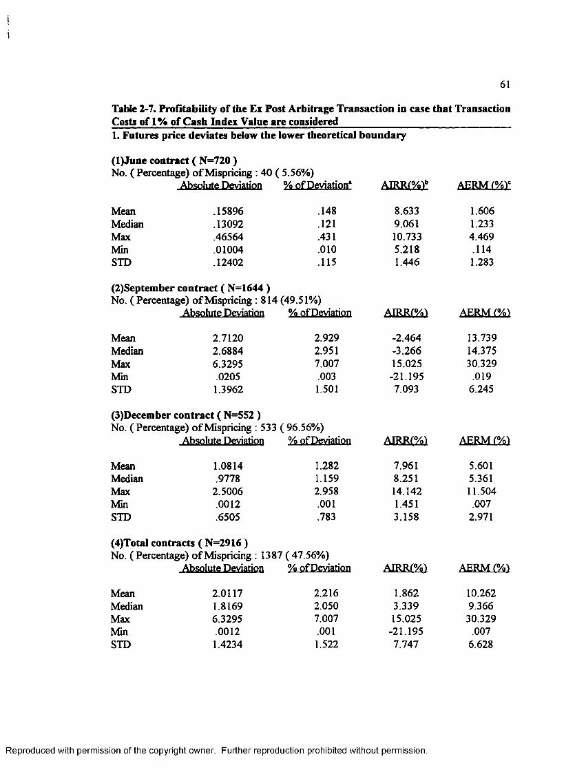
i
i
61
Table 2-7. Profitability of the Ex Post Arbitrage Transaction in case that TransactionCosts of 1% of Cash Index Value are considered_______________________________1. Futures price deviates below the lower theoretical boundary
(l)June contract ( N=720)No. ( Percentage) o f Mispricing : 40 ( 5.56%)
Absolute Deviation % of Deviation* AJRR(%)b AERM (%)c
Mean .15896 .148 8.633 1.606Median .13092 .121 9.061 1.233Max .46564 .431 10.733 4.469Min .01004 .010 5.218 .114STD .12402 .115 1.446 1.283
(2)September contract ( N=1644 )No. ( Percentage) of Mispricing : 814 (49.51%)
Absolute Deviation % of Deviation AIRRf%l AERM (%)
Mean 2.7120 2.929 -2.464 13.739Median 2.6884 2.951 -3.266 14.375Max 6.3295 7.007 15.025 30.329Min .0205 .003 -21.195 .019STD 1.3962 1.501 7.093 6.245
(3)December contract ( N=552)No. ( Percentage) of Mispricing : 533
Absolute Deviation( 96.56%)
% of Deviation AIRR(%) AERM(%)
Mean 1.0814 1.282 7.961 5.601Median .9778 1.159 8.251 5.361Max 2.5006 2.958 14.142 11.504Min .0012 .001 1.451 .007STD .6505 .783 3.158 2.971
(4)Total contracts ( N=2916 )No. ( Percentage) of Mispricing : 1387 ( 47.56%)
Absolute Deviation % of Deviation AIRR/%1 AERM (%)
Mean 2.0117 2.216 1.862 10.262Median 1.8169 2.050 3.339 9.366Max 6.3295 7.007 15.025 30.329Min .0012 .001 -21.195 .007STD 1.4234 1.522 7.747 6.628
Reproduced with permission of the copyright owner. Further reproduction prohibited without permission.

ti
62
Table 2-7. Continued ____
2. Futures price deviates above the upper theoretical boundary
(l)June contract ( N=720)No. ( Percentage) of Mispricing : 0 ( 0.00%)
(2) September contract ( N=1644)No. ( Percentage) of Mispricing : 162 ( 9.85%)
Absolute Deviation % of Deviation AIRR/%1 AERM (%)
Mean .2510 .298 22.265 7.669Median .2044 .243 20.665 6.074Max .6608 .784 36.925 24.585Min .0050 .006 15.084 .164STD .1761 .115 5.165 5.809
(3) December contract ( N=552 )No. ( Percentage) of Mispricing : 0 ( 0.00%)
(4) Total contracts ( N=2916 )No. ( Percentage) of Mispricing : 162( 5.56%)
* The percentage of mispricing is computed by dividing absolute deviation of futures price from its theoretical lower ( or upper) boundary after accounting for 1% transaction cost with the lower ( or upper )boundary value.b Annualized implied repo rate (AIRP) is calculated by the following formulas.
REPO, = ( 365/N )[ In {F,/[ S, ( 1- ) - PV( Div,)]}] if F, < F,REPO, = ( 365/N )[ In {F, /[ S, ( 1+ ) - PV( Div,)]}] if F, > F ,
where PV( Div, ) = present value of dividends paid on spot between t and T (=Ei=1T-<DHj e x p ^ 5))
N= time to expiration (T-t)0Annualized expected excess return to maturity (AERM) is calculated by the following formulas.
if F, > F+, , ( 365/ N)/ [ ( actual futures price - upper bound)/ arbitrage capital)] if F, < F",, ( 365/ N)/ [ ( lower bound - actual futures price)/ arbitrage capital)]
Reproduced with permission of the copyright owner. Further reproduction prohibited without permission.

{
s
63
Table 2-8. Profitability of the Ex Post Arbitrage Transaction in case that TransactionCosts of 2% of Cash Index Value are considered_______________________________1. Futures price deviates below the lower theoretical boundary
(l)June contract ( N=720)No. ( Percentage) o f Mispricing : 0 ( 0.00%)
(2)September contract ( N=1664)No. ( Percentage) of Mispricing : 702 ( 42.19%)
Absolute Deviation % of Deviation* AIRR(%)b a e ™ (%y
Mean 2.1335 2.325 .907 11.414Median 2.1521 2.373 .853 11.395Max 5.4171 6.058 12.692 28.112Min .0201 .022 -16.445 .155STD 1.1470 1.251 5.833 5.627
(3)December contract ( N=552)No. ( Percentage) of Mispricing : 295
Absolute Deviation( 53.44%)
% of Deviation AIRR(%) AERM (%)
Mean .7029 .849 10.427 3.719Median .6032 .737 10.908 3.340Max 1.6465 1.967 14.368 8.188Min .0004 .000 5.709 .002STD .4794 .577 2.408 2.373
(4)Total contracts ( N=2916)No. ( Percentage) of Mispricing : 997 (34.19%)
Absolute Deviation % of Deviation AIRR('%'> AERM (%)
Mean 1.7102 1.888 3.724 9.138Median 1.4754 1.673 4.736 7.947Max 5.4171 6.058 14.368 28.112Min .0004 .000 -16.445 .002STD 1.192 .577 6.675 6.055
2. Futures price deviates above the upper theoretical boundaiyThere is no case for the entire period in which futures price rises beyond the upper boundaryof theoretical pricing band when 2% hedge costs are accounted for.
Reproduced with permission of the copyright owner. Further reproduction prohibited without permission.
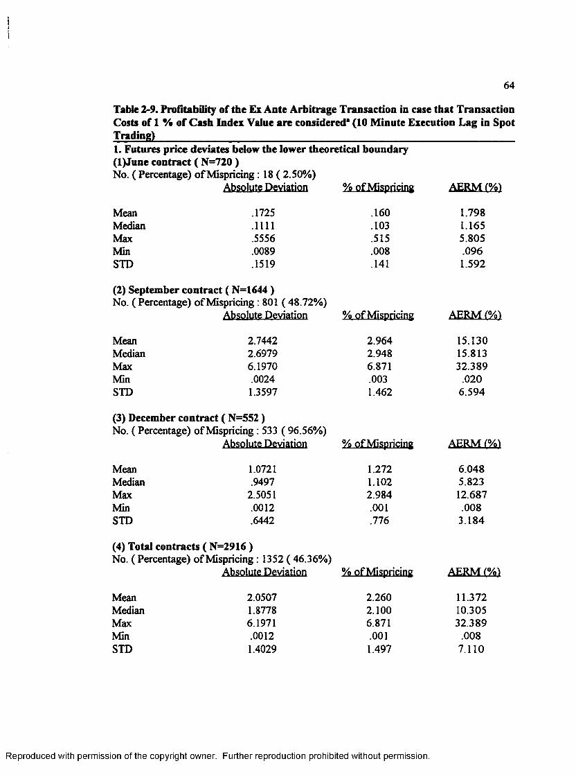
iti
64
Table 2-9. Profitability of the Ex Ante Arbitrage Transaction in case that Transaction Costs of 1 % of Cash Index Value are considered* (10 Minute Execution Lag in SpotTrading)_________________________________________________________________1. Futures price deviates below the lower theoretical boundary (l)June contract ( N=720 )No. ( Percentage) of Mispricing: 18 ( 2.50%)
Absolute Deviation % of Mispricing AERM f%)
Mean .1725 .160 1.798Median .1111 .103 1.165Max .5556 .515 5.805Min .0089 .008 .096STD .1519 .141 1.592
(2) September contract ( N=1644)No. ( Percentage) of Mispricing: 801 ( 48.72%)
Absolute Deviation % of Mispricing AERM (%)
Mean 2.7442 2.964 15.130Median 2.6979 2.948 15.813Max 6.1970 6.871 32.389Min .0024 .003 .020STD 1.3597 1.462 6.594
(3) December contract ( N=552)No. ( Percentage) of Mispricing : 533 ( 96.56%)
Absolute Deviation % of Mispricing AERM (%)
Mean 1.0721 1.272 6.048Median .9497 1.102 5.823Max 2.5051 2.984 12.687Min .0012 .001 .008STD .6442 .776 3.184
(4) Total contracts ( N=2916)No. ( Percentage) of Mispricing : 1352 ( 46.36%)
Absolute Deviation % of Mispricing AERM (%)
Mean 2.0507 2.260 11.372Median 1.8778 2.100 10.305Max 6.1971 6.871 32.389Min .0012 .001 .008STD 1.4029 1.497 7.110
Reproduced with permission of the copyright owner. Further reproduction prohibited without permission.

1?I1
65
Table 2-9. continued_______________________________________________________1. Futures price deviates above the upper theoretical boundary
(1)June contract ( N=720)No. ( Percentage) of Mispricing : 0 ( 0.00%)
(2) September contract ( N=1644)No. ( Percentage) of Mispricing : 138 ( 8.39%)
Absolute Deviation % of Mispricing AERM (%)
Mean .2788 .331 7.493Median .2534 .301 6.541Max .6309 .738 18.729Min .0023 .003 .068STD .1504 .178 4.293
(3) December contract ( N=552)No. ( Percentage) of Mispricing : 0 ( 0.00%)(4) Total contracts ( N=2916)No. ( Percentage) of Mispricing : 138 ( 4.73%)
1 The ex ante test of arbitrage profitability is conducted by investigating whether the ex post deviation from the arbitrage free band would be still profitable after considering 10 minute delay in executing the arbitrage transaction. 1% transaction costs are assumed to be incurred in this arbitrage.
Reproduced with permission of the copyright owner. Further reproduction prohibited without permission.

66
Table 2-10. Profitability of the Ex Ante Arbitrage Transaction in case that Transaction Costs of 2 % of Cash Index Value are considered* (10 Minute Execution Lag in SpotTrading)_________________________________________________________________1. Futures price deviates below the lower theoretical boundary
(1)June contract ( N—720 )No. ( Percentage) of Mispricing: 0 ( 0.00%)(2)September contract ( N=1664 )No. ( Percentage) of Mispricing : 700 ( 42.07%)
Absolute Deviation % of Mispricing AERM (%)
Mean 2.1262 2.318 11.373Median 2.1847 2.423 11.452Max 5.2862 5.920 27.473Min .0095 .011 .073STD 1.1399 1.243 5.650(3) December contract ( N=552 )No. ( Percentage) of Mispricing : 273 ( 49.46%)
Absolute Deviation % of Mispricing AERMI%)
Mean .7394 .894 3.896Median .7027 .857 3.800Max 1.6571 1.994 8.344Min .0026 .003 .017STD .4612 .554 2.275(4) Total contracts ( N=2916 )No. ( Percentage) of Mispricing : 973 ( 33.47%)
Absolute Deviation % of Mispricing AERM (%)
Mean 1.7371 1.918 9.275Median 1.4702 1.680 8.162Max 5.2860 5.920 27.473Min .0026 .003 .017STD 1.1758 1.268 5.975
2. Futures price deviates above the upper theoretical boundaryThere is no case for the entire period in which futures price rises beyond the upper boundaryof theoretical pricing band when 2% hedge costs are accounted for.__________________1 The ex ante test of arbitrage profitability is conducted by investigating whether the ex post deviation from the arbitrage free band would be still profitable after considering 10 minute delay in executing the arbitrage transaction. 2% transaction costs are assumed to be incurred in this arbitrage.
Reproduced with permission of the copyright owner. Further reproduction prohibited without permission.

Iit
67
Table 2-11. Profitability of the Ex Ante Arbitrage Transaction in case that Transaction Costs of 1% of Cash Index Value are considered* ( 10 Minute Execution Lag in FuturesTrading)_________________________________________________________________1. Futures price deviates below the lower theoretical boundary (l)June contract ( N=720 )No. ( Percentage) o f Mispricing : 32 ( 4.44%)
Absolute Deviation % of Mispricing AERM (%)
Mean .3219 .301 3.356Median .2846 .265 3.041Max .6554 .606 10.734Min .0398 .038 .416STD .1707 .159 2.154
(2) September contract ( N=1644)No. ( Percentage) of Mispricing : 807 ( 49.09%)
Absolute Deviation % of Mispricing AERM (%)
Mean 2.7401 2.959 13.884Median 2.7374 3.004 14.554Max 6.4295 7.118 30.808Min .0032 .004 .025STD 1.3944 1.498 6.203
(3) December contract ( N=552 )No. ( Percentage) of Mispricing : 516 (93.48%)
Absolute Deviation % of Mispricing AERM (%)
Mean 1.1162 1.323 5.776Median .9956 1.190 5.382Max 2.7361 3.227 12.458Min .0216 .025 .143STD .6628 .797 3.043
(4) Total contracts ( N=2916 )No. ( Percentage) of Mispricing : 1355 ( 46.47%)
Absolute Deviation % of Mispricing AERM (%)
Mean 2.0646 2.273 10.548Median 1.8393 2.082 9.542Max 6.4295 7.118 30.808Min .0032 .004 .025STD 1.4183 1.515 6.563
Reproduced with permission of the copyright owner. Further reproduction prohibited without permission.

1i
68
Table 2-11. Continued_____________________________________________________1. Futures price deviates above the upper theoretical boundary
(1)June contract ( N=720 )No. ( Percentage) of Mispricing : 0 (0.00%)
(2) September contract ( N=1644)No. ( Percentage) of Mispricing : 140 ( 8.52%)
Absolute Deviation % of Mispricing AERM (%)
Mean .3057 .364 8.496Median .2704 .319 6.876Max .8108 .982 27.152Min .0003 .000 .005STD .2177 .261 6.632
(3) December contract ( N=552)No. ( Percentage) of Mispricing : 0 (0.00%)(4) Total contracts ( N=2916 )No. ( Percentage) of Mispricing :140 ( 4.80%)
1 The ex ante test of arbitrage profitability is conducted by investigating whether the ex post deviation from the arbitrage free band would be still profitable after considering 10 minute delay in executing the arbitrage transaction. 1% transaction costs are assumed to be incurred in this arbitrage.
Reproduced with permission of the copyright owner. Further reproduction prohibited without permission.

69
Table 2-12. Profitability of the Ex Ante Arbitrage Transaction in case that Transaction Costs of 2% of Cash Index are considered* (10 Minute Execution Lag in FuturesTrading)_________________________________________________________________1. Futures price deviates below the lower theoretical boundary
(1)June contract ( N=720 )No. ( Percentage) of Mispricing : 0 ( 0.00%)(2)September contract ( N=1664 )No. ( Percentage) of Mispricing : 692 ( 41.59%)
Absolute Deviation % o f Mispricing AERM (%)
Mean 2.1693 2.364 11.596Median 2.2164 2.458 11.695Max 5.5171 6.170 28.631Min .0095 .011 .073STD 1.1450 1.248 5.655(3) December contract ( N=552)No. ( Percentage) of Mispricing : 273 ( 49.46%)
Absolute Deviation % of Mispricing AERM (%)
Mean .7707 .929 4.085Median .7095 .867 3.942Max 1.879 2.240 9.268Min .0038 .005 .021STD .487 .587 2.410(4) Total contracts ( N=2916)No. ( Percentage) of Mispricing : 965 ( 33.09%)
Absolute Deviation % of Mispricing AERM (%)
Mean 1.7737 1.958 9.471Median 1.5491 1.754 8.419Max 5.5171 6.170 28.631Min .0038 .005 .021STD 1.1848 1.277 6.002
2. Futures price deviates above the upper theoretical boundaryThere is no case for the entire period in which futures price rises beyond the upper boundaryof theoretical pricing band when 2% hedge costs are accounted for.___________________1 The ex ante test of arbitrage profitability is conducted by investigating whether the ex post deviation from the arbitrage free band would be still profitable after considering 10 minute delay in executing the arbitrage transaction. 2% transaction costs are assumed to be incurred in this arbitrage.
Reproduced with permission of the copyright owner. Further reproduction prohibited without permission.
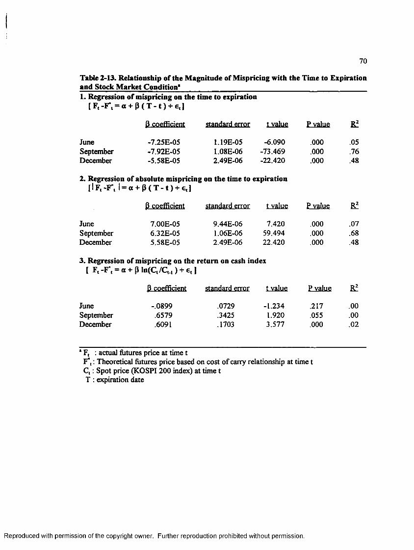
I
70
Table 2-13. Relationship of the Magnitude of Mispricing with the Time to Expirationand Stock Market Condition*_______________________________________________1. Regression of mispricing on the time to expiration
[ Ft -F*t = a + P ( T - 1 ) + et ]
P coefficient standard error t value P value El
June -7.25E-05 1.19E-05 -6.090 .000 .05September -7.92E-05 1.08E-06 -73.469 .000 .76December -5.58E-05 2.49E-06 -22.420 .000 .48
2. Regression of absolute mispricing on the time to expiration[IFt -F \ 1 = a + P ( T - t ) + € j
P coefficient standard error t value P value El
June 7.00E-05 9.44E-06 7.420 .000 .07September 6.32E-05 1.06E-06 59.494 .000 .68December 5.58E-05 2.49E-06 22.420 .000 .48
3. Regression of mispricing on the return on cash index[ Ft -F \ = a + P In(Ct /C,_,) + e, ]
P coefficient standard error t value P value El
June -.0899 .0729 -1.234 .217 .00September .6579 .3425 1.920 .055 .00December .6091 .1703 3.577 .000 .02
* Ft : actual futures price at time t F*t : Theoretical futures price based on cost of carry relationship at time t Ct : Spot price (KOSPI200 index) at time t T : expiration date
Reproduced with permission of the copyright owner. Further reproduction prohibited without permission.
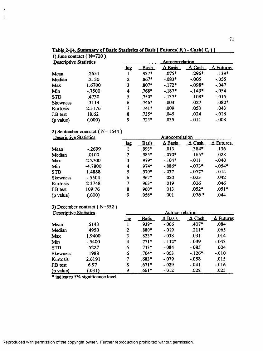
I1»
71
Table 2-14. Summary of Basic Statistics of Basis f Futures( F,) - Cash( C ,) |1) June contract ( N=720 )Descriptive Statistics AutocorrelationA/WJVUyilTV
lag Basis A Basis. A Cash A FuturesMean .2651 1 .937* .075* .296* .139*Median .2150 2 .867* -.083* -.005 -.055Max 1.6700 3 .807* -.172* -.098* -.047Min -.7500 4 .768* -.187* -.149* -.054STD .4730 5 .750* -.137* -.108* -.015Skewness .3114 6 .746* .003 .027 .080*Kurtosis 2.5176 7 .741* .009 .053 .043J.B test 18.62 8 .735* .045 .024 -.016(p value) (.000) 9 .723* .035 -.011 -.008
2) September contract ( N= 1644 )DescriDtive Statistics Autocorrelation
lag Basis _A.Rasis_ A Cash A FuturesMean -.2699 1 .993* .013 .384* .136Median .0100 2 .985* -.070* .165* .028Max 2.2700 3 .979* -.104* -.011 -.040Min -4.7800 4 .974* -.086* -.073* -.054*STD 1.4888 5 .970* -.037 -.072* -.014Skewness -.5504 6 .967* .020 -.023 .042Kurtosis 2.3748 7 .963* .019 .026 .046J.B test 109.76 8 .960* .013 .052* .051*(p value) (.000) 9 .956* .001 .076 * .044
3) December contract ( N=552 )Descriotive Statistics Autocorrelation
lag Basis A Basis .A .Cash. A FuturesMean .5143 1 .939* -.006 .407* .084Median .4950 2 .880* -.019 .211* .065Max 1.9400 3 .823* -.038 .031 .014Min -.5400 4 .771* -.132* -.049 -.043STD .5227 5 .733* -.084 -.085 .004Skewness .1988 6 .704* -.063 -.126* -.010Kurtosis 2.6191 7 .683* -.079 -.058 .015J.B test 6.97 8 .671* -.029 -.041 -.016(p value) (.031) 9 .661* -.012 .028 .025* indicates 5% significance level.
Reproduced with permission of the copyright owner. Further reproduction prohibited without permission.

*
72
Table 2-15. Monthly Trading Profile of Futures Contract over the Sample Periods (May 3,1996 ~ Oct.31,1996)______________________________________________Month Volume
( Contracts)Value
( Won Bil.)Open Interest ( Contracts)
Arbitrage Trade Contract Value
(Won Bil.)
May 83,330 4,367 38,192 - -
June 68,169 3,182 60,480 965 44.3July 72,669 3,233 126,206 444 19.6August 79,492 3,306 144,348 344 15.1September 87,200 3,626 104,788 251 10.5October* 118,935 5,079 142,481 396 17.1Year Total 509,795 22,793 616,495 2,400 106.6Daily Average 3,444 154 4,166 16.2 0.72Source : Korea Stock Exchange* The above table offers the total tally of the entire October month for comparison purpose even though our sample covers only up to 16th of October.
Reproduced with permission of the copyright owner. Further reproduction prohibited without permission.

Cha
rt
2-1.
Tr
end
of Fu
ture
s M
ispri
cing
(A
s of
cash
In
dex)
SUH9661-
01019661 S001-9661 09609661 12609661 Z1-609661. 1-1-609661- 90609661- 20609661- Z2809661- 22809661- L 1-809661- 21-809661' Z080966I- 20809661- 62Z0966L *2Z0966I 81-109661- 2 LZ09661- 80Z09661-
80Z0966I 82909661- *2909661- 61-909661. * 1-909661- Z090966I 80909661- 82909661- 22909661- L 1-909661. 81-909661- 80909661- 80909661-
CSI CM m co oo o>
Reproduced with permission of the copyright owner. Further reproduction prohibited without permission.

Cha
rt
2-2.
A
nnua
lized
Im
plied
Re
po
Rat
es
O'QL
91-01-966I6001-9661.3001-9661.*3609661-61-609661.£1-609661.90609661-30609661-93809661-33809661-91-809661.01-809661-90809661-1-8Z0966I93Z09661- ~(Q03Z09661- °9LZ09661-60Z0966 V80Z0966I83909661-*3909661-81-909661.1-1-909661.90909661-08909661-93909661-81-909661-*1-909661-80909661£0909661-
Reproduced with permission of the copyright owner. Further reproduction prohibited without permission.

S K) 19661 01-01.9661. *0019661 09609661 02609661 91609661- 01609661.
90609661- 09909661- 92909661 12809661
91809661. 60809661 90809661192.09661 92209661222.09661 91209661 01109661 90209661
102.09661 92909661
02909661 91909661 01909661 90909661 62909661 92909661
2.1909661 91909661 80909661 90909661
in o m o m o m o m•«- i - o o o > o ) o o o o r ^ -t — r - i — t -
JUjOd xspui
Reproduced with permission of the copyright owner. Further reproduction prohibited without permission.
(Aoocotso(O(0
o2+*coo(0ffi
3LL
C0)Eo>oCJo•cQL
■NrSB
S 3
Dat
e
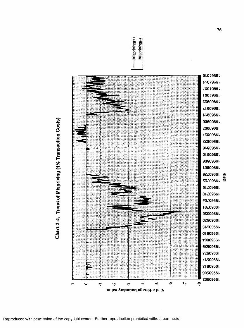
Cha
rt 2
-4.
Tren
d of
Misp
rici
ng
(1%
Tra
nsac
tion
Cos
ts)
76
a> ratc c :o o i*n:Q. 0.1(O tn i5 si
r
9101.9661
I-1019661
ZOO 1-966 L
1.001-9661
€3609661
L 1.609661.
1.1.609661
90609661-
30609661
Z3809661-
33909661.91.809661.
01.809661
90809661-
1.0809661.
93Z.09661
33Z0966I
91Z0966L
0 L£0966L
604)9661
104)966 L 93909661.
03909661.
91.909661.01.909661.
*0909661.
63909661-
€3909661.
I I-909661- €1-909661.
80909661.
€0909661.cm co ^ ml i l t
an|BA Ajepunoq aBejp.qje jo
Reproduced with permission of the copyright owner. Further reproduction prohibited without permission.
Date

Cha
rt 2
-5.
Price
M
ovem
ent
of Fu
ture
s C
ontr
act
( 2%
Tra
nsac
tion
Cos
t)
77
Sl-01-9661
0KH966L
MO 1-9661. 09609661
03609661.
91-60966 L
01609661
90609661.
09909661-
93909661.
1-3909661
91.909661
60909661.
90909661.
1-9109661
93109661.
33109661
SH0966I.
01109661.
9010966I
I-0109661.
93909661-
03909661-
9L909661.
01909661.
90909661-
63909661-
33909661-
II-909661.
31-909661.
90909661- 30909661-
m o m o m o t n o m t- t- o o o> o> c o e o r ' .
jujod xapui
tni P .w (J3 W2 S. SI S i
3 -
Reproduced with permission of the copyright owner. Further reproduction prohibited without permission.
Dat
e

Cha
rt 2
-6.
Tren
d of
Misp
rici
ng
(2%
Tra
nsac
tion
Cos
ts
78
£ 3 !a ) 0)1c c ;o 0 i
*c 1o . a(O CO
S 2
I!9 to 19661-
11019661
ZOO 19661(-001-966I.
93609661-
Z1609661
1 (609661-
90609661.
30609661-
Z380966 1
33809661.
91809661.
01809661.
90809661
10809661
93Z09661
33Z09661
91Z09661
01Z09661
S0Z09661
10Z09661
93909661
03909661
S 190966101909661
>0909661
63S09661
£3509661
Z1S09661£1509661
80509661£0509661
CM ID COa n |B A A j e p u n o q a B e j p q j e j o %
Reproduced with permission of the copyright owner. Further reproduction prohibited without permission.
Dat
e

CO(0O
COp
3U.CO’<0(0m**-o■o
■«Nkj98
91.01.966I
i. 1.01.9661-
1001-9661.
1001.9661. £3609661- 91-60966 L
£1.609661.
10609661
£0609661.
63809661
*3809661
03809661- * 1.809661. 60909661
80809661
I-£109661-
93109661.
3310966I-
91.109661.
1.1.109661. 90109661.
30109661.
13909661.
33909661.
81.909661.
31.909661.
10909661-
1-0909661.
83809661-
33809661-
11.809661-
£1.809661.
80809661.
£0809661.
luiod xapui
Reproduced with permission of the copyright owner. Further reproduction prohibited without permission.

80
CHAPTER III
LEAD AND LAG RELATIONSHIP IN PRICE CHANGES
BETWEEN CASH AND FUTURES MARKETS
3-1. Literature Review
Black (1976) argues that the greatest benefit earned from the existence of futures
market is neither risk hedging nor allocation of risk, but rather its side effect: a discovery of
price by which market participants can make a corporate decision. Grossman (1989) also
emphasizes the role of price discovery by the futures market that transmits information from
informed traders to the uninformed. He argues that the futures market tends to develop if and
only if informed traders will profit from their information and some of that information is not
transmitted to the uninformed traders by equilibrium spot prices. In contrast, in an efficient
capital market where all available information is fully and instantaneously utilized to determine
the market price of capital asset, futures price should move concurrently with its
corresponding spot price without any lead and lag in price movements from one market to
the other.
Due to the market frictions such as transaction costs or the capital market
microstructure effects, however, significant lead and lag relationship between two markets
is frequently observed. In the U.S. market, it is generally documented that futures price leads
cash prices due to differences in speed of adjustment to the new information, which result
from differences in transaction costs, asynchronous trading in cash prices and etc. Herbst,
McCormick and West (1987) find that index futures prices tend to lead those of their cash
Reproduced with permission of the copyright owner. Further reproduction prohibited without permission.

81
indices for both Value Line and S&P 500, but the spot index adjusts so quickly (on average
less than one minute) that knowledge of the lead and lag relationship can not be used for
profitable trading opportunity. Finnerty and Park (1987) explain the chain of causality from
futures to cash in program trading in the following way : Initially, when investors expect the
stock price to rise, they first buy futures because there is no initial investment and low
transaction costs. Imbalance between futures and underlying cash index prices occurs
subsequently due to a rise in futures price. Then, the gap between futures and stock prices is
reduced due to the simultaneous sale of futures and purchase of the underlying index in the
program trading. They maintain that internal factors such as changes in investor expectation
or external factors such as interest rate changes will cause the change in spread between
futures and spot, which in turn, affect the lead-lag relationship. In the early introduction
period of index futures for both MMI and MMMI (especially before 1986), however, they
find little correlation between change in the futures price and subsequent change in the index.
As the futures market matures, futures price changes strongly lead spot index changes in their
study. Garbade and Silber (1983) and Ng (1987) insist that inter-relationship between spot
prices and future prices depends on the supply of arbitrage services between the two markets.
Garbade and Silber (1983) argue that if the supply of arbitrage services is perfectly elastic,
futures contract will be a perfect substitute for a cash market position and each will follow
a common random walk. Ng (1987) suggests that when arbitrage transactions are costly (the
supply of arbitrage service is not perfectly elastic), then one market may lead or lag the other
in reflecting new information and that the lower costs of transacting in the futures market
make the futures markets more informationally efficient than their corresponding spot
Reproduced with permission of the copyright owner. Further reproduction prohibited without permission.

82
markets.29 Using daily data, she finds that lead-lag relationship does not persist for more than
one day due to possible arbitrage between two markets and even though futures prices lead
spot prices for the stock indexes and some currency futures, the small magnitudes of cross
correlation between lagged futures price and spot prices make it difficult for the uninformed
traders to earn excess profits using this relationship. She also asserts that the harder the
instantaneous arbitrage strategies are implemented, i.e., the more stocks a spot index is
comprised with, the more salient a lead and lag relationship is present between two markets.30
Kawaller, Koch and Koch (1987) document that S&P 500 futures price and the index are
simultaneously related throughout the trading day31. But they also find that the lead from
futures to cash prices persists for over twenty minutes while the reverse relationship does not
last for more than one minute. They attribute this stronger “futures leading spot”relationship
to the infrequent trading in the stock market. Herbst, et al. (1987) call it “ wait to be traded”
feature of a spot index. If the market makes a significant move, some of the stock in the index
will not yet have traded and the index based in part on pre-move prices of less actively traded
stocks will under represent the true index value. In this regard, Fleming, Ostdiek and Whaley
29 She argues that transaction costs are more binding in hindering arbitrage activities especially in case of short sale due to margin requirement and uptick rule.
30 She observes a stronger causal relationship for the Value Line index than for the S&P 500 index. Herbst etc. (1987) also document that S&P 500 stock index reacts faster (in 8 minutes) to changes in futures price than Value Line index does ( in 16 minutes). They argue that the more volume of trading is and the less number o f securities in basket are, the faster spot index adjusts to the changes in futures contract price.
31 They observe that the magnitudes of the contemporaneous coefficients overwhelm all lag coefficients in both directions, indicating that futures and spot prices move largely in tandem.
Reproduced with permission of the copyright owner. Further reproduction prohibited without permission.

83
(1996) observe that the S&P 100 index more strongly leads the S&P 500 stock index. With
the greater trading frequency of S&P 100 stocks relative to S&P 500 stocks, S&P 100 have
less serious asynchronous trading problems than S&P 500. However, infrequent trading in
spot index alone does not seem to explain the observed strong lead from futures price to spot
index value. Stoll and Whaley (1990a) report that index futures lead their spot prices by about
five to ten minutes even after purging microstructure effects such as infrequent trading and
bid-ask bounces. But they also find some evidence that spot returns lead futures returns in the
early inception period of futures trading. Consistent with Kawaller, et al.(1987), they report
that returns in the futures and spot markets mostly move contemporaneously. Chan (1992)
also suggests that information adjustment is faster for futures than for cash index due to the
staleness of component stock prices by asynchronous trading and less costly transaction costs
in futures market.32 After controlling non-synchronous trading, he also find an asymmetric
lead and lag relationship between the two markets with strong evidence that futures leads the
cash index and only weak evidence that the cash index leads the futures. In addition, he adds
that cash index prices lag futures not only under bad news but also under good news33 and,
32 He suggests three factors as the possible determinants of the lead and lag relations between futures and spot market. First, restrictions on short sale in spot market slow the adjustment of prices to private information, especially with respect to private bad news. Hence, futures prices without short sale constraints should lead the cash index to a greater degree under bad news. Second, the lead-lag relationship may be affected by the intensity of trading activity in the two markets while price discovery and trading activity are related. Third, the futures market should reflect market-wide information more quickly than cash market does.
33 He hypothesizes that due to the short sale restrictions such as uptick rule and the resulting greater execution risk, spot respond more slowly to futures price change under bad news than under good news. However, he does not find any stronger tendency for the
Reproduced with permission of the copyright owner. Further reproduction prohibited without permission.
84
more importantly that when there are more stocks moving together, the feedback from the
futures market to the cash market is stronger. Moreover, he documents that futures return
leads not only cash index return, but also individual stock return such as IBM. Since IBM is
a more frequently traded stock than index futures and has no serious infrequent trading
problem, his result suggests that microstructure effects alone can not account for strong lead
from futures to cash. He concludes that the futures market becomes the main source of
market-wide information while the cash market is the main source of firm-specific
information. Similarly, Subrahmanyam (1991) insists that stock index futures provide a
preferred trading medium for uninformed liquidity traders who wish to trade portfolios
because adverse selection costs (incurred in trading against informed traders) are lower in the
stock index futures market than in markets for individual securities. He argues that the
independent orders submitted by informed traders in the basket tend to offset each other when
the number of securities comprising the basket is large. He adds that this diversification
benefit reduces the transaction costs of the liquidity traders and improves their terms of trade
against informed traders when they trade in the basket. Therefore, uninformed liquidity
traders and traders with only market wide information migrate to invest in the stock index
futures market while informed traders prefer to invest in individual securities. This will cause
stock index futures market to reflect more rapidly market wide information.
In terms of volatility interaction between cash and futures market, Kawaller, Koch and
Koch (1990) do not observe any systematic pattern of lead and lag relationship in volatilities
futures to lead the cash index under bad news than under good news.
Reproduced with permission of the copyright owner. Further reproduction prohibited without permission.

85
between two markets34, in contrast to the lead and lag relationship in price changes between
two markets. In line with Kawaller, et al. (1990), Chan and Chan, Karolyi (1991) report that
price innovations in either the cash or futures market influence the volatility in the other
market, suggesting that while the lead and lag relationship in returns is almost unidirectional
or asymmetric (futures leading cash), that of volatility is bi-directional or symmetric. They
also note that although the lead and lag relations between the price changes of the cash and
futures markets appears to diminish over the sample period35, the inter-market dependence
of volatility grows stronger and comparably in both directions. As Ross (1989) argues that
price volatility is directly related to the rate of information arrival, their evidence is consistent
with the hypothesis that new market information disseminates in both the futures and stock
markets, and that both markets serve important price discovery roles. They suggest that new
information that hits either markets can, in general, predict the arrival rate of information in
the other market. Chan and Chung (1993) also document similar bi-directional volatility
movements that over 1984-85, MMI index futures price volatility is preceded by volatility in
the underlying spot index and current spot volatility is strongly correlated with past futures
price volatility. However, they report that there is asymmetry in the economic magnitude of
the respective lead and lag relationship and that the lead from futures volatility to cash
34 They find that the volatility relationships are not robust across different contract periods with index volatilities leading futures volatility in some sample periods (1985) and the reverse movements in the other period (1986). They also argue that even though future prices lead spot prices, lagged volatilities in spot prices could influence the futures price volatilities.
35 Over the two subsample periods (1985-1986, 1988-1989), they do not find significant lead from cash to futures but observe that the impact of cash market return shocks and past cash market volatility on the futures market volatility is even stronger than usual.
Reproduced with permission of the copyright owner. Further reproduction prohibited without permission.

\
86
volatility is stronger than the opposite direction. Lee and Linn (1994) also report that
causality in volatility runs in both directions for S&P S00 futures and index despite evidence
of stronger lead from futures return to spot return. Similarly, Cheung and Ng (1990,1996)
document strong feedback (simultaneous interaction) in volatilities between S&P 500 futures
and spot index although there is evidence of the direction of causality running from futures
price volatility to cash price volatility during the first 15 minute trading.
As for empirical studies conducted in other countries, these report different empirical
results regarding the lead and lag relations of returns and volatilities between futures and
stock markets. Abhyankar (1995) tests the lead and lag relationship in returns and volatility
between the FT-SE 100 stock index futures and the underlying cash index using hourly
intraday data. He finds a strong contemporaneous relationship between the FT-SE futures and
cash market along with some significant evidence of futures leading cash market, especially
during times of high volatility. It is noted, however, that the sizeable reduction in transaction
costs in the London equity market after Big Bang made the size and the significance of the
lead of the futures returns over the index returns decrease. However, he does not find any
clear pattern of one market leading the other in terms of volatility. He observes strong
contemporaneous volatility interaction between futures and cash markets, but lead and lag
relationship in volatility are changed according to the sample period. This result is consistent
with earlier evidence in the U.S. market such as Kawaller, et al. (1990) and Chan, et al.
(1991). Alternatively, Shyy, Vijayraghavan and Scott-Quinn (1996) find the reverse causality
from cash (CAC cash index) to futures (CAC futures contract) in the French market when
asynchronous trading problem is resolved by using the midquote points of bid-ask prices, even
Reproduced with permission of the copyright owner. Further reproduction prohibited without permission.

87
though they find the lead-lag relationship from futures to cash when the minute by minute
transaction data is used. They conclude that previous results showing futures leading cash
may be primarily due to market asynchronous trading and stale price problems, as well as
differences in trading mechanisms used in cash or futures markets. Lim (1992) observes that
the futures price movements on Nikkei Stock Average (NSA) futures contract are highly
positive correlated with contemporaneous spot price movements within five minute intervals.
However, beyond contemporaneous comovements, no apparent lead and lag relationship is
found between returns for futures contract on SIMEX and returns for cash index on the
Tokyo market. Iihara, Kato and Tokunaga (1996) report that Nikkei Stock Average (NSA)
futures return strongly leads cash returns, but that no bidirectional volatility feedbacks in
volatility between futures returns and cash returns are not observed in Japan, contrary to the
results reported by Chan, Chan and Karolyi (1991). Instead, they observe that futures market
shocks are transmitted significantly to the volatility of the cash market, not in the opposite
way. Martikainen, Perttunen and Puttonen (1995) investigate the lead and lag relationship
between futures contract and individual stocks or between cash index and individual stocks
in the Finnish market. They insist that futures market returns predict the returns of most
stocks, traded both infrequently and frequently, better than the cash index returns do. Since
the most frequently traded stocks are led by futures market returns at least as clearly as the
portfolio of infrequently traded stocks, they conclude that the asynchronous trading of
component stock prices does not seem to be a dominant factor, making it appear that futures
prices lead cash index prices. In the Australian market, Gannon (1994) finds uni-directional
volatility movement from futures to cash.
Reproduced with permission of the copyright owner. Further reproduction prohibited without permission.

88
In summary, different samples (contracts) have different results about lead and lag
relationship, but most of the previous studies suggest that the lead and lag relationship
between futures and spot returns is asymmetric or uni-directional. On the other hand,
volatility transmissions between two markets are bi-directional. Knowledge of this
relationship between two markets, however, can not be exploited for making excess returns
since the arbitrage activities will soon eliminate such profitable opportunities, bringing the
cost of carry relation back into alignment.36
3-2. Data and Methodology
3-2-1. Data Description
Due to the computerization of arbitrage transactions and the program trading, the data
needs to be sampled on an intradaily rather than daily basis in order to detect an economically
meaningful causal relationship. In our study, we are using 10 minute intraday data from May
3rd through October 16th, covering 2715 ten minute intraday returns, 112 session break
returns (sampled over 1 hour and 40 minutes) and 132 overnight returns for KOSPI 200
index, KOSPI index and the nearby futures contract.37 In addition to the lead and lag
36 Stoll and Whaley (1990a) and Fleming, Ostdiek and Whaley (1996) suggest that growth in stock market volume, increasing efficiency of index arbitrage and programing trading execution make a contemporaneous relationship between futures and cash markets stronger with less lead and lag relationship as time passes. This indicates a continued integration of the index futures and stock market.
37 Most previous studies omit the overnight returns, because they are sampled over different time interval. However, unlike the U.S., Korean stock market has intermission between morning and afternoon session, and this causes another complexity for conducting time series using intraday data. Since our data covers 10 minute intraday data, lack of sample size inevitably made us to rely on the other method (see Kawaller, Koch
Reproduced with permission of the copyright owner. Further reproduction prohibited without permission.

89
relationship in returns and volatility between KOSPI200 index and futures, those between
KOSPI index and futures or between two stock indexes are also examined to differentiate the
effects of price movement of the large cap stocks on the lead-lag relationship from those of
the small cap stocks. This investigation can also test Chan’s (1992) market wide information
hypothesis. Each of the return series is constructed as continuous compounding percentage
returns by taking natural logarithm on the ratio of current price to the lagged price and
multiplying this by 100. Following Kawaller, Koch and Koch (1990),Cheung and Ng (1990)
and Chan,Chan and Karolyi (1991), we control overnight returns and session break returns
from 10 minute intraday returns by dummy variables. It is well documented that new
information arrives and accumulates even during the non-trading hours, which affects the
returns during trading hours. Since there is a disparity in futures price before and after each
of the expiration dates o f the nearby contract, we divide the total sample into three periods
according to the life of the nearby futures contract.
Table 3-1 displays the descriptive statistics for each of stock index return and its
nearby futures contract. For 10 minute intraday returns, their means and medians are not
positive except for futures return in December throughout the entire sample period. This
mainly results from the unfavorable stock market condition during our sample period. To
reflect the inertia in trading for the early inception period, the median return of futures
contract is zero for the whole contract period. Over the entire period, futures volatility
(standard deviation) is greater than those for spot market indexes and between two stock
indexes, volatility of KOSPI 200 is greater than that for KOSPI. Infrequent trading of
and Koch 1990 ; Cheung and Ng 1990).
Reproduced with permission of the copyright owner. Further reproduction prohibited without permission.

Ii
90
component stocks (especially small sized stocks) seems to dampen return volatility, while the
volatility is relatively higher during June contract period than over September or December
contract periods for both stock indexes, futures returns are more volatile over September or
December contract periods than over June contract period. Chan and Chung (1993) and
Chen,Cuny and Haugen (1995) report that large mispricing in futures price results in an
increase in supply of arbitrage services and an increase in volatility in both futures and cash
markets.This increase in volatility subsequently reduces mispricing of futures contract.
However, they suggest that when stocks are moving downward and futures contracts are
underpriced, this relationship becomes attenuated. Therefore, it is observable that lack of
arbitrage capital reduces stock market volatility over the September and December contract
periods whereas more volatile stock market condition (due to active arbitrage activities)
makes future price move relatively well in line with cost of carry relationship over June
contract period. For all return series, Jarque-Bera normality test rejects the null hypothesis
of normal distribution.
Table 3-2 summarizes the same descriptive statistics for session break returns. Except
for futures contract, the session break returns are on average positive for stock indexes. It is
noticeable that the standard deviation of the session break return is not so much higher or
over some periods lower than the 10 minute intraday returns for all return series.38 Unlike 10
38 If stock or futures price follows random walk process, the variance of the return (differenced log price) increases proportionately with sample interval. Therefore, in theory, the standard deviation of session break return or overnight return should be greater than 10 minute intraday return by multiples o f / 10 and / i l l . However, previous studies (French and Roll 1986 etc.) document that overnight return’s volatility is not so much high as the theory dictates.
Reproduced with permission of the copyright owner. Further reproduction prohibited without permission.

I
91
minute intraday returns, the normality is satisfied for all of session break returns except for
KOSPI 200 index over September contract period. As shown in the Table 3-3, overnight
returns are larger in magnitude than 10 minute returns or session break returns and take on
positive value on average for stock indexes. On the contrary, for fUtures contract, overnight
returns are more negative and larger in magnitude than the session break return or intraday
returns. The volatility (standard deviation) for overnight returns are approximately three
times greater than the 10 minute intraday returns or session break returns for all of stock
index and futures return series.
3-2-2. Methodologies in Lead and Lag Relationship Study
In terms of methodological breakdown for previous studies, Herbst, McCormick and
West (1987), Ng(1987), Kawaller, Koch and Koch (1987),Chan,Chan and Karolyi (1991)
and Cheung and Ng (1996 ) employ the sample cross-correlations between future returns and
cash returns to check the lead and lag relationship. Kawaller, Koch and Koch (1987, 1990),
Finnerty and Park (1987), Stoll and whaley (1990a), Chan (1992), Chan and Chung (1993,
1995), Koch (1993), Lee and Lin (1994), Gannon (1994), Martikainen, Perttunen and
Puttonen (1995) and Fleming, Ostdiek and Whaley (1996) use the Granger causality test39 to
39 Granger causality (X, causes Yt in Granger sense) implies that the past information of X, contributes to the lower variance of prediction of Yt than without that information.That is, consider two stationary and egordic time series, X, and Y( and let be I, and Jt be two information sets defined by I, = { X,.j; j ^ 0 } and Jt = { X,.j, Y,.j; j * 0 }. Y, is said to cause X,+1 in variance if E{ ( X,+1 - f | I , } * E{ ( X1+l - p ^ f | J , }, where p ^ , is the mean o f X,+1 conditioned on I , . Feedback in variance occurs if X, causes Y, and Y, causes X, There is instantaneous causality in variance if E{ ( X,+1 - p^1+1 )21 J ,} *E{ (X,+l - p^l+, )21 Jt+Y,+1 }, see more details in Ng (1987) and Cheung and Ng (1996).
Reproduced with permission of the copyright owner. Further reproduction prohibited without permission.

92
identify the uni or bi-directional movements in returns and volatilities between futures and
cashes.40 In addition, Chan, Chan and Karolyi (1991) use the bivariate GARCH model to
explore the volatility spillover effects between futures and cashes. In line with the previous
studies, we apply various regression techniques based upon the Granger causality concept
in our analysis of lead and lag relationship in returns and volatility between stock indexes and
futures contract.
3-2-3. Dynamic Simultaneous Equations Model (SEM) and Vector Autoregression
Model (VAR)
To test the temporal price relationship between the index and its nearby futures
contract, the Granger or Sims causality test is frequently employed in the previous literature.
Suppose two time series, {Y,} and (X t }. The series X, fails to Granger cause Yt if in a
regression of Y, on lagged Y’s and lagged X’s, the coefficients of the latter are zero. That is,
K = t - t P, X,-. ♦ e,-----------------------------------(3-1)/=l (=1
Then if p; = 0 (I = 1,2,.... , k), X, fails to cause Y, The lag length k is , to some extent
arbitrary. Alternatively, Sims (1972) includes the current and future terms of X, as well as
40 While their approaches are fundamentally similar in checking the possible causal relationships, Kawaller, Koch and Koch (1987,1990), Koch (1993) insist on using the dynamic simultaneous equations model (SEM) that includes the contemporaneous returns (or volatilities) in the right-hand side as well as the left hand side of the equation system. Chan and Chung (1993, 1995), on the other hand, argue that including such contemporaneous terms in the equations may be misleading in interpretation of the causality and that the vector autoregression (VAR) is preferable.
Reproduced with permission of the copyright owner. Further reproduction prohibited without permission.

{
i
93
lagged X, in a regression of Yt. Sims says that Yt fails to cause X, in the Granger sense if
in a regression of Yt on lagged, current, and future X, , the latter coefficients are zero.
Consider the regression,
K = E * E P ,* , , * ----------------0 - 2 )J -- o r - 1
and test Pj = 0 ( j=l,2,.... ,k). This says that the prediction of Y from current and past X’s
would not be improved if futures values are included. Although there are some econometric
differences between two tests, they basically test the same hypothesis (e.g., see Geweke,
Meese and Dent 1983 and Maddala 1992). To investigate the inter-dependence between two
time series (in our case, stock index and its corresponding futures price) based upon the above
mentioned two causality notions, we employ several estimation techniques used in financial
literatures. In our study, dynamic simultaneous equations model (SEM, see Kawaller, Koch
and Koch 1987) using three stage least squares (3SLS) estimation method is first applied on
our data set to see if futures and cash prices may affect each other contemporaneously. If two
series are concurrently correlated, OLS estimation would result in inconsistent and inefficient
estimation. Three stage least squares (3SLS)extends two stage least squares technique by
taking into account cross equation correlation and yields more efficient parameter estimates
than 2SLS. Dynamic simultaneous equations model in our study can be written as follows.
Reproduced with permission of the copyright owner. Further reproduction prohibited without permission.

94
~ C1 + ^ If-k + ^ Pi* r-Jfc +eif k=1 k=0P <7
Ft ~ c2 + ]ET ®2Jfc f-fc + X) Pit Ffk +C:
*(3-3)
2/*=0 Jt=l
where e lt and €* are contemporaneously correlated.
The order of lag p and q is somewhat arbitrary and determined in our study by cross
correlation function and Akaike information criterion (AIC) value. We test whether sum of
coefficients of a ’s and P’s in each equation is equal to zero to interpret the lead and lag
relationship between futures and spot market movements. The Wald test is applied for joint
coefficient restriction and its test value is calculated by the following way.
_ ( SSEr - SSEf ) ____________* SSEp / (T-k- l)
Where SSE^ SSEp = residual sum of squares of the reduced and full models, respectively
T = total number of observations,
k = number of lagged series I ,, Ft
The Wald test statistic follows x-distribution with degree of freedom k.
Vector autoregression (VAR) was developed by Sims (1980) and originally contrived
to avoid any structural restrictions on the parameter estimation by treating all variables as
endogenous. It requires minimal theoretical demand on the structure of the model. This
original VAR model can be estimated by OLS since there are no unlagged endogenous
variables on the right-hand side, and since the right-hand side variables are the same in each
Reproduced with permission of the copyright owner. Further reproduction prohibited without permission.
95
equation, OLS is a consistent and efficient estimator. However, the efficiency of the original
VAR model might be improved by using Zeilner’s seemingly unrelated regression method
(SUR), because SUR takes explicit account of cross equation correlation by transforming the
equations to minimize the correlation across residuals. Chan and Chung (1993), however,
argue that the reduced model (VAR) and the simultaneous equation model (SEM) are just
simple transformations of each other and so one does not contain information that the other
does not. Since we analyze the lead and lag relationship between cash and futures markets
using common data set for SEM and VAR estimations, VAR and SEM should basically
deliver consistent message regarding price movements between cash and futures markets.
3-2-4. Cointegration Test
Two economic variables are said to be cointegrated when a linear combination of the
two variables is stationary even though each variable is non stationary. In other words, yt is
integrated of order 1; y,=I (1), that is, the first differencing makes y, stationary and another
time series variable x, is I (1) then if there is a nonzero coefficient p such that y, - Px, is I (0),
y, and x, are said to be cointegrated. If y, and x, are not cointegrated, i.e., z ,, a combination
of two time series, yt and x, is also 1(1), then two variables y, and x, can drift apart from each
other more and more as time goes on so that there would be no long run equilibrium
relationship between them. Alternatively, if the system between two economic variables is
moving toward equilibrium, economic theory suggests that the long run relationship between
x, and yt should beyt= Pxt and the equilibrium error z, = y, - Px, In order to test whether the
series x, and y, are cointegrated, it is necessary to establish that each series is I (1), i.e., each
Reproduced with permission of the copyright owner. Further reproduction prohibited without permission.

96
has a unit root in its autoregressive representation. Test for the presence of a unit root is
performed by conducting the augmented Dickey-Fuller (ADF) test (1979).
The augmented Dickey-Fuller (ADF) test is modified version of Dickey-Fuller (DF)
test by adding sufficient terms in Ax,.,- to account for autocorrelations in residual e(. We run
the above regression and test whether the coefficient p is zero (x , is non-stationary). If the
ADF test on series can not reject the null hypothesis of existence of a unit root, we
subsequently conduct the ADF test on first differenced time series to identify the second unit
roots and so on. The t statistics on coefficient p do not follow the normal t distribution and
can be expressed as integrals of Brownian motions, (see Engle and Yoo 1987). This
distribution is skewed to the left and has most of its mass below zero reflecting the fact that
values of p greater than zero could have generated a particular data set only with very low
probability. Once it is found that each series contains a single unit root, i.e., 1(1), it will be
checked to see whether the two series are cointegrated. In the first step, residuals (z,) are
obtained by running OLS regression on two time series x, and y ,: = c , + Pyt + z, . In the
next step, the augmented Dickey-Fuller(ADF) test is conducted on these residual series z, to
determine that residuals follow stationary movements. If the two series x, and y are
cointegrated, the z, will be 1(0).
A*f = a0 + pXt_y + £ + e,7=1
(3-5)
(3-6)
Reproduced with permission of the copyright owner. Further reproduction prohibited without permission.

i
97
The t ratio from this test, however, no longer has the Dickey-Fuller distribution since
the cointegrating coefficient p has been estimated and therefore makes the residual series
appear slightly more stationary than if it were computed at true p.41 Engle and Granger
(1987) show that if two series are cointegrated, they are necessarily represented by an error
correction model (ECM) such as equations 3-7.
AX, = p,Z,., ♦ lagged( A X, AY, ) ♦ e„ ----------- (3-7)
AY, = pjZ,., ♦ lagged^ AX, AY, ) * e„
where eH, e* are white noise and at least one of pt , p2 is non zero.
If x, and yt are cointegrated, then each component of each equation is I (0), and so the
equations are balanced. Error correction model (ECM) includes both short run and long run
information in modeling the time series. It relates the change in x, (Ax,) to the change in y,
(Ay,) and the past period’s disequilibrium (z^,). In equation 3-7, z, is a measure o f the extent
to which the system is out of long run equilibrium, and thus called the equilibrium error. The
next change in x, and y,will be influenced by the size and sign of the current equilibrium error.
It can be noted that if there is a period with no shocks, so that e*, are zero, the system will
41 The distribution of this test is called the Engle-Granger distribution and MacKinnon (1991) provides more precise critical values based on 25,000 simulation experiments. According to his tables, the estimated critical value for any number of observation T can be calculated using the following equation.
c(p,T)= p. + p,rl + p2r 2 where p and T stand for significance level and sample size, and all beta values are asymptotic critical values in his tables. See more details in MacKinnon (1991).
Reproduced with permission of the copyright owner. Further reproduction prohibited without permission.

98
converge so that A x, ,Ayt both go to zero, so that the points ( x ,, yt) converge so that they
lie on the line x, = (iyt The error correction equations may be thought of as the disequilibrium
mechanism that guides the economy to the equilibrium ( see Engle and Granger 1991). The
test for causality between two series x, and yt is based on an Wald statistic that is calculated
by estimating the above ECMs in both unrestricted (foil model) and restricted (reduced
model) forms.
3-2-5. Treatments Regarding Infrequent Trading Effect, Overnight and Session Break
Returns
In the first stage of specifying the structure of return dynamics for each asset, we first
take into account the microstructure effects such as asynchronous trading and bid-ask bounce
on the lead and lag relationship between futures and cash market since these microstructure
effects may lead to the spurious results regarding interpretation of the possible lead and lag
relationship. Stoll and Whaley (1990a) employ ARMA(2,3) filtering to account for
microstructure effects. Chan (1992), Miller, Muthuswamy and Whaley (1994) argue that
asynchronous trading problem in the stock index can be reasonably approximated by the first
order autoregressive model (AR(1)). They insist that bid and ask bounces are not significant
for stock index because they are canceled out in the middle of combining the constituent
stocks into a single stock index. In contrast, futures price shows relatively low and
insignificant autocorrelation and hence is usually used in its raw returns for analysis or the first
order moving average model (MA(1)) is applied to control the bid -ask bounces. On the other
hand, Jokivuolle (1995) demonstrates that the observed stock index can be represented by a
Reproduced with permission of the copyright owner. Further reproduction prohibited without permission.

riI
99
standard infinite order MA process, which can be readily represented as an ARMA(p,q)
according to the Wold decomposition. He insists that Beveridge-Nelson permanent
component42 of the observed index process equals the true index level and that the true stock
index value may be assessed by eliminating infrequent trading effects by filtering the observed
index value with the first order moving average (MA(1)) model.43 Similarly, the first order
moving average (MA(1)) model is employed to capture the effect of non-synchronous trading
by French, Schwert and Stambaugh (1987) and Hamao, Mauslis and Ng (1990). In
consideration of the spurious results the infrequent trading of component stocks in the stock
index may cause to the lead and lag relations between cash and futures market, our study
investigates Granger causal relationship using both unfiltered raw return series and pre
whitened return series. Since our sample covers overnight returns and session break returns
as well as 10 minute intraday returns, pre-whitening procedure using ARMA specification
should be applied to the 10 minute raw returns while simultaneously controlling for these
returns based on longer time span. Chan, Chan and Karolyi (1991) and Kawaller, Koch and
Koch (1990) note that new information continues to accumulate during non-trading hours and
is likely to influence the time series process of intraday returns over trading hours. Therefore,
in addition to treatments for non-synchronous trading effects in stock indexes, our sample
controls for overnight and session break returns using dummy variables and applying transfer
42 For more details about Wold decomposition (1938) and Beveridge and Nelson (1981), see Time Series Analysis (1994) by Hamilton, J.D., p.p. 108 -109 and p.p.504-505.
43 For example, suppose that the log difference of the observed index, R,0 = X,° - X,.1°can be estimated by the MA(1) process such as R,0 = p + 0, e,.,0 + et° , the Beveridge-Nelson permanent component or the log of the true index level equals X,° + 0, et°.
Reproduced with permission of the copyright owner. Further reproduction prohibited without permission.

function (or ARMAX ) on the raw returns as follows:
100
Rt = c 0 + c1dSB + + <|>'1 (L)0 (L)et -------------------------------- (3-8)
where
(j)'1 (L) = 1/ ( 1 - <J>! L - ........ - 4>p Lp ) for autoregressive representation (AR) of order p
0 (L) = (1 - 0,L - ........ - 0pLq) for moving average representation (MA) of order q
L = lag operator
dgB = dummy variable taking on value of one for overnight return and, zero otherwise
d„ = dummy variable taking on value of one for session break return, and zero otherwise
In this transfer function specification (3-8), a regression model using dummy variables is first
constructed to control for overnight returns and session break returns and then an ARMA
model is developed to remove infrequent trading effect or bid-ask bounce effect from the
residual series in the regression equation. All parameters in both regression equation and
ARMA equations are simultaneously estimated. In our study, alternative ARMA models
should be tested on the each stock index return or futures return to select the most
parsimonious return specification. Akaike Information Criteria (AIC) are used in selection
of the order of ARMA terms and Ljung-Box Q test is conducted to insure white noise of
residual return series.
Reproduced with permission of the copyright owner. Further reproduction prohibited without permission.

i
Ii
101
3-2-6. Volatility Structure
Following Schwert (1989,1990), we use the absolute value of return innovation (or
residuals) employed in the Granger causality test of the conditional returns as a proxy for
return volatility to investigate volatility structure between futures and cash markets. Each
either futures return or stock index return.44 Again, VAR model is applied to the relationship
between contemporary volatility and its lagged own and other market’s volatility as follows:45
Davidian and Carroll (1987) insist that estimates of standard deviation based on absolute
value transformation of residuals are more robust to departures from normality than are
variables for overnight and session break volatility are included as exogenous variables in the
44 If residuals ( unexpected return) follows normal distribution, ie, ~ N( 0, o 2), then mean absolute residual E(| e, | ) = (2/ it )* a
45 VAR model is employed in many studies to estimate the multivariate volatility structure. For example, Schwert (1989), Battacharya and Sundaran (1986), Chatrath, Ramchander and Song (1995) and Huang, Mauslis and Stoll (1996).
absolute residual is multiplied by (re /2 )* and this figure estimates the standard deviation of
where | U, | = V(k/2) x | e, | (3-9)
et = return innovation obtained after ARMA filtering and
controlling for session break and overnight return in equation (3-8)
squared residuals. In line with the return dynamics analysis, trading volumes and dummy
Reproduced with permission of the copyright owner. Further reproduction prohibited without permission.

Ii
102
VAR system.
3-3. Empirical Results regarding Lead and Lag Relationship between Cash andFutures
3-3-1. Analyses of Sample Correlations
Table 3-4 shows autocorrelation coefficients for the stock indexes and futures returns
over the three futures contract periods. As the Ljung-Box Q statistics at lag 10 suggest, all
of the return series do not follow white noise process except for futures returns over the
December contract period. For both KOSPI and KOSPI 200 index returns, the first order
autocorrelation is positive and strong as the theory predicts. Except for December contract
period, the first and second order autocorrelation coefficients are slightly higher for KOSPI
than for KOSPI 200. This is consistent with infrequent trading effect theory because KOSPI
encompasses smaller stocks than KOSPI 200 so that spurious positive autocorrelation the
non-synchronous trading causes is more salient in KOSPI. The first order autocorrelation for
stock indexes becomes larger in magnitude over the sample period. It indicates that non-
synchronous trading problem in the cash market becomes more serious. It is also observable
that futures contract also has a positive first order autocorrelation in the Korean market. In
most of previous studies (MacKinlay and Ramaswamy 1988 ; Miller, Muthuswamy and
Whaley 1994) in the U.S. market, they find that futures contract has a close to zero
autocorrelation or if any, negative autocorrelation as the bid -ask bounce at order flows
predicts. However, for those studies about futures markets in other countries, significantly
positive first order autocorrelation is commonly observed ( For example, see Iihara, Kato and
Tokunaga 1996 for Japan market; and Abhyankar 1995 for the U.K. market). As seen in
Reproduced with permission of the copyright owner. Further reproduction prohibited without permission.

103
Tables 3-1,3-2 and 3-3, futures contract shows negative return throughout the whole trading
or non trading hours. The inertia in the futures market due to lack of arbitrage capital or
weak stock market condition may contribute to the positive linear dependency in futures
returns. Therefore, futures returns also need to be filtered by the appropriate ARMA
specification before examining the lead and lag relationship between cash and futures.
Table 3-5 displays the cross correlation coefficients between stock index and futures
returns, or between two stock index returns. While the contemporaneous correlation seems
to be the strongest for each pair of returns, it is apparent that futures returns tend to lead the
stock index returns over the whole periods since the lagged futures return is more frequently
and strongly correlated with the current stock index returns than the opposite way. Although
it is less clear in lead and lag relationship in terms of cross correlation function between
KOSPI 200 and KOSPI, the magnitude (or significance) is stronger when the lagged KOSPI
200 returns are matched with the current KOSPI returns than the case where the lagged
KOSPI returns are correlated with the current KOSPI 200 returns. Therefore, it can be said
that KOSPI 200 leads KOSPI weakly.
3-3-2. Results of Prewhitening
Table 3-6 shows how much different overnight returns and session break returns are
from the mean of 10 minute intraday returns over the sample periods. Except for futures
returns which show little difference in overnight or session break returns from the intraday
10 minute returns, the overnight and session break returns of the stock market indexes turn
out to be significantly higher than the comparable average 10 minute returns. This result is
Reproduced with permission of the copyright owner. Further reproduction prohibited without permission.

104
consistent with Wood, Mclnish and Ord (1985) and Ekman’s (1992) studies. It confirms the
needs to control for overnight and session break returns in our sample. In Table 3-7,
appropriate ARMA specifications are presented for removing any spurious autocorrelation
in each of return series of the stock index and futures contract. Using ARMAX (transfer
function), the dummy variables for overnight and session break returns are simultaneously
controlled. To insure that return innovations (residuals) are white noise procedure, Ljung-
Box Q test is conducted at lag 20. The result shows that whitening of residuals is successfully
achieved.
3-3-3. Results of Simultaneous Equation Model (SEM) and Vector Autoregression
(VAR)
Table 3-8 presents the results of parameter estimation by simultaneous equations
model (SEM) using 3SLS. In each pair of series, regressions are run both on raw returns
without whitening and on the residuals after whitening. Besides the return series, variables
proxying for trading volume are included in the system. Following Chan and Chung (1993),
the logarithmic transformed volume within 10 minute interval is used as proxy for trading
volume. The number of lags in the regression system is determined by the Akaike Information
Criteria (AIC). For Granger causal relationship between KOSPI 200 and futures contract, the
Wald statistic indicates that a bilateral lead and lag relationship between futures and KOSPI
200 was observed during June and September contract periods. However, the strength of the
Granger causality is stronger when futures leads KOSPI 200 than when KOSPI 200 leads
futures. Over December periods, KOSPI 200 no longer leads the futures while futures still
Reproduced with permission of the copyright owner. Further reproduction prohibited without permission.

ttI
I
105
strongly lead KOSPI 200. One striking feature is that unlike cross correlation, the current
futures returns do not move together with the KOSPI 200 returns. Rather, lagged futures
returns have stronger explanatory power in variation in the movement o f KOSPI returns. For
lead and lag relationship between futures and the wider stock market index, KOSPI does not
Granger cause the futures except over the June contract period where a bilateral lead and lag
relationship is present. Again, the lagged returns of futures are more strongly related to the
current KOSPI movement. Between two stock indexes, KOSPI 200 always leads KOSPI
strongly over the whole sample periods whereas the KOSPI never Granger cause KOSPI 200
at all. Bessembinder, Chan and Seguin (1996) argue that trading of large capitalization stocks
is more closely associated with market-wide news than is that of small capitalization stocks.
However, unlike relationship with futures, the concurrent movement is present between
movements of two stock index returns. Overall, these results also support Chan’s (1992)
argument that futures price reflects the market wide information more rapidly than the stock
index and are consistent with Bessembinder, Chan and Seguin’s (1996) finding in that larger
stocks (mostly constituents of KOSPI 200) reflect this information faster than the small stocks
(represented by KOSPI).
In Table 3-9, results of vector autoregression (VAR) estimation are presented. In this
estimation, the concurrent terms are omitted from the regression system. Generally, the
estimation results of VAR model are similar to those of the SEM estimation. Futures strongly
lead both KOSPI 200 and KOSPI over the entire sample periods. However, a bilateral lead
and lag relationship between either o f stock indexes and futures is also present except for
December contract periods, although lead from stock indexes to futures is relatively weak
Reproduced with permission of the copyright owner. Further reproduction prohibited without permission.

106
compared to the lead from future to the stock indexes. Again, KOSPI 200 strongly leads
KOSPI while the opposite way does not hold. Over the whole sample period, the volume has
negative impact on the returns of futures contract, indicating that heavy transactions tend to
push futures price downward.
3-3-4. Results of Cointegration
Table 3-10 presents the results of unit root tests for stock indexes and futures price.
Unit root tests are conducted on the logarithmic transformed price series. ADF tests indicate
that all of price series are the first order non-stationary, i.e., the first differencing makes them
stationary. In Table 3-11, cointegration tests are run on each pair of stock index and futures
return series to see if there is any long run equilibrium relationship between them.
Theoretically, there should be a long run relationship among them since cost of carry
relationship dictates futures price to move in tandem with stock price and KOSPI 200 is a
subset of KOSPI. Strikingly, over the whole sample periods, the null hypothesis of no
cointegration can not be rejected between KOSPI and KOSPI 200 at any conventional
significance level. Some answer can be found for this disparity between two stock indexes by
examining the trend of returns of large cap stocks and small cap stocks over the sample
period. In Table 3-12, the monthly returns of large cap stocks , medium cap stocks and small
cap stocks are presented. As is clearly seen from the table, large cap stocks suffer more from
the capital loss than the medium cap stock or small cap stocks. Since the KOSPI 200 is
composed of mainly large cap stocks, the market downturn would have effected differential
impact on the KOSPI and KOSPI 200, leaving the equilibrium relationship between two
Reproduced with permission of the copyright owner. Further reproduction prohibited without permission.

107
indexes temporarily broken over the sample period. Except for September contract period
where deviation of futures price from the cost of carry relationship is severe, futures and each
of stock indexes interact with each other along their long run price relationship.
Table 3-13 displays the results of error correction model (ECM) raised by Engle and
Granger (1987). They are similar to the VAR model except that ECM includes error
correction terms (Z,.,) in its equation system. Their results are basically the same as those
obtained from VAR or SEM in that futures strongly lead stock indexes although in some
periods, a bilateral lead and lag relationship between cash and futures markets is observed.
Consistent with cointegration results from ADF tests, error correction term (Z,.,) is
statistically significant and negative for each pair of KOSPI 200 and futures or KOSPI and
futures except for September contract. This indicates that deviation from the long run
equilibrium relationship would affect the returns of stock index or futures and make them
revert to the equilibrium relationship.
3-3-5. The Extent of Stock Market Co-Movement by Market-Wide Information
Chan (1992) develops a few proxy variables to measure the extent of market-wide
movement. One of these variables is measured by | Nu - Nd | / ( Nu + Nd + Nz), where Nu,
Nd, and Nz are the number of stocks moving upward, moving downward, and with no change.
This proxy variable measures the net proportion of stocks moving together. The higher the
ratio is, the more likely there is market-wide information affecting the stocks moving
together. Whenever the stock market is moved by the market-wide information, futures prices
react to those information faster than do cash prices, and the feedback from the futures
Reproduced with permission of the copyright owner. Further reproduction prohibited without permission.

108
market to the cash market is stronger. Table 3-14 displays the daily mean and median ratios
of this proxy variable over the sample period. By construction, this proxy variable takes on
zero value when the number of stocks moving upward is equal to the number of stocks
moving downward. Suppose that the ex ante probabilities of stocks moving upward,
downward, and without price change are all equal, and then if the number of stocks moving
in one direction is twice as many as that of stocks moving in the opposite direction, the ratio
takes on .222. Again, if the number of stocks moving in one direction is three times greater
than that of stocks moving in the opposite direction, the ratio has a value of .333. In our
sample, the average (median) value of this ratio is .279 (.269). This means that on daily basis,
the number of stocks moving in one direction is on average about 2.5 times greater than the
number of stocks moving in the opposite direction. This result clearly indicates the clustering
of stocks moving in same direction over the sample period and supports Chan’s (1992)
hypothesis in that over the sample period, the Korean stock market is moved by the market-
wide information and futures market reflects such information faster than does spot market.
Moreover, as Bessembinder, Chan and Seguin (1996) insist, large capitalization stocks are
more likely affected by market-wide information than small sized stocks. This high ratio is
also consistent with our result that KOSPI 200 strongly leads KOSPI.
3-3-6. Lead and Lag relationship in Volatility
In Table 3-15, lead and lag relationships in volatility among stock indexes and futures
are presented. As a volatility measure, absolute residuals from ARMA specifications
(transformed by multiplying by / (n/2)) are used. Unlike Granger causality relationships
Reproduced with permission of the copyright owner. Further reproduction prohibited without permission.

109
observed in the return series, volatility causality results in mixed outcomes. For KOSPI 200
and futures, futures volatility Granger causes only KOSPI 200 volatility over the June
contract period. Throughout September and December contract periods, neither KOSPI 200
nor futures contract leads the other. On the other hand, strong ARCH (autoregressive
heteroscedasticity) effects are observed in KOSPI 200 over the entire sample periods and for
futures during September contract period. Volatility tends to persist for both stock index and
futures over September contract period. It is noticeable that for KOSPI and futures,
significant bilateral causality is found over the sample period except during December
contract period. ARCH effects are also prevalent in KOSPI. For KOSPI 200 and KOSPI,
results are really mixed depending upon the sample period. Over the June and September
contract periods, volatility of KOSPI 200 returns weakly leads volatility of KOSPI while
during December contract period, KOSPI leads KOSPI 200. In addition, ARCH effect of
KOSPI is diminished by volatility spillover effect from KOSPI 200 over the September
contract period. In contrast, ARCH effect of KOSPI 200 is offset by the effect from lagged
volatility of KOSPI during December contract period. In line with previous studies (for
example, Karpoff 1987 ; Lamoureux and Lastrapes 1990), trading volume has significantly
positive relationship with volatilities for all return series throughout the overall period, which
is in contrast with the results found in return causality relationship. Consistent with Kawaller,
Koch and Koch (1990), both futures and index volatility increase directly with futures trading
volume, even stronger effect on stock index volatility than stock index volume itself. This
result indicates either that greater futures activity ( arbitrages or unwinding force) produces
greater stock price volatility or that higher stock market volatility requires a greater reliance
Reproduced with permission of the copyright owner. Further reproduction prohibited without permission.

I!
110
on futures for risk management Overall, bilateral volatility causality relations are found in the
Korean market, which is consistent with previous studies regarding other markets.
3-4. Conclusion
In this chapter, possible lead and lag relationships in returns and volatilities between
cash and futures market are investigated. Granger causality test is extensively undertaken with
several regression system methodologies including SEM, VAR and ECM. For returns
relationship, futures market tend to strongly lead cash market by as long as 30 minutes.
Results of SEM suggest that lagged futures returns explain more of variation in cash returns
than contemporaneous futures returns. However, from time to time, it is also observed that
spot market leads futures market. Between two stock indexes, KOSPI 200 has a strong
tendency to lead KOSPI, the wider index. The above two results concerning returns causality
test are basically consistent with previous studies conducted in the other market. As Chan
(1992) hypothesizes, futures reflect more rapidly market wide information than spot market,
and large cap stocks adjust faster to new information in the market than small cap stocks.
Even after removing spurious positive autocorrelation in the stock returns, the above lead and
lag relationships are basically unchanged. Regarding volatility interaction between cash and
futures markets, results suggest that unlike lead and lag relationship in returns, a bi-directional
causality is more prevalent between cash and futures market, and its relationship entirely
depends on the sample period and spot index used. This fact is also consistent with earlier
empirical studies in the other market. Unlike their impact on returns, trading volumes in each
market have significant explanatory power in changes in volatility with a more strong effect
Reproduced with permission of the copyright owner. Further reproduction prohibited without permission.

I l l
of futures volume on the spot volatility as Kawaller, Koch and Koch (1990) document.
Overall, market friction such as transaction costs and short sale restriction seem to hinder spot
market from reacting faster to the new information than futures market.
Reproduced with permission of the copyright owner. Further reproduction prohibited without permission.

112
Table 3-l.Summary Statistics for Intraday 10 Minute Returns on the KOSPI 200 Index Futures and the KOSPI 200 Stock Index, and the KOSPI Stock Index from May 3, 1996 to Oct.16,1996_______________________________________________________
1. KOSPI 200 Futures Statistic Jun. Sep. Dec. TotalSample size 681 1528 506 2715Mean -.02166 -.00194 .00579 -.00545Median .00000 .00000 .00000 .00000Std. Dev. .16273 .22703 .21528 .21061Skewness -.06661 .71473 .00569 .52631Kurtosis 4.63549 11.11816 3.54757 9.62781J-Q statistic 76.40 4326.01 6.32 5094.67( p- value)______________ (,00)________ £00)________£04)__________(.00)
2. KOSPI 200 stock index Statistic Jun. Sep. Dec. TotalSample size 681 1528 506 2715Mean -.02892 -.01001 -.01139 -.01501Median -.02800 -.01157 -.01227 -.01855Std. Dev. .17377 .14720 .16282 .15734Skewness .15990 .34107 .31175 .25491Kurtosis 3.84652 5.56285 4.30839 4.77614J-Q statistic 23.24 447.80 44.29 386.27( p- value) (.00) (-00) (-00) (.00)
3. KOSPI stock indexStatistic Jun. Sep. Dec. TotalSample size 681 1528 506 2715Mean -.02628 -.01031 -.00969 -.01420Median -.02125 -.01221 -.00904 -.01387Std. Dev. .16232 .13708 .14576 .14552Skewness .15902 .27032 .23805 .20659Kurtosis 3.72780 5.16461 4.10663 4.52001J-Q statistic 17.90 316.92 30.60 280.68( p- value) ..COPI. . . (.00) (-00) (-00)Under the null hypothesis of normality for return series, skewness(m3) and kurtosis (m4) are asymptotically distributed as m3 ~ N( 0, 6/T) and m4 ~ N (3, 24/T), where T is the number of observations. The J-Q (Jarque-Bera) statistic tests whether a series is normally distributed. Under the null hypothesis of normality, the J-Q statistic is distributed x2 with 2 degrees of freedom.
Reproduced with permission of the copyright owner. Further reproduction prohibited without permission.

Table 3-2. Summary Statistics for Session Break Returns (1 hrs and 40 min.) on the KOSPI 200 Index Futures and the KOSPI 200 Stock Index, and the KOSPI Stock
a a v a u
1. KOSPI 200 Futures Statistic Jun. Sep. Dec. TotalSample size 28 63 21 112Mean .01976 -.03377 .03219 -.00802Median -.02363 -.05481 .00000 .00000Std. Dev. .15953 .18097 .32906 .21183Skewness .54783 .16094 .52902 .62436Kurtosis 2.75070 3.00518 2.85272 4.52145J-Q statistic 1.47 .27 1.00 18.08( p-value) (46) (-87) (.61) (.00)
2. KOSPI 200 stock indexStatistic Jun. Sep. Dec. TotalSample size 28 63 21 112Mean .06654 .00529 .09688 .03778Median .05837 -.01130 .09915 .00000Std. Dev. .18630 .14574 .22508 .17579Skewness .82645 .74657 .69928 .96528Kurtosis 3.22775 4.16411 2.75627 4.08660J-Q statistic 3.25 9.41 1.76 22.90(p-value) (.20) (.01) (.41) (.00)
3. KOSPI stock indexStatistic Jun. Sep. Dec. TotalSample size 28 63 21 112Mean .06478 .00461 .10114 .03775Median .04324 .00000 .08688 .01337Std. Dev. .18025 .14081 .20202 .16703Skewness .51859 .51849 .53425 .71061Kurtosis 2.60925 4.0170 2.62475 3.60043J-Q statistic 1.43 5.54 1.12 11.11(p-value) 1-49JL. (.06) (.57) (-00)Under the null hypothesis of normality for return series, skewness(m3) and kurtosis (m4) are asymptotically distributed as m3 ~ N( 0, 6/T) and m4 ~ N (3, 24/T), where T is the number of observations. The J-Q (Jarque-Bera) statistic tests whether a series is normally distributed. Under the null hypothesis o f normality, the J-Q statistic is distributed x2 with 2 degrees of freedom.
Reproduced with permission of the copyright owner. Further reproduction prohibited without permission.

114
Table 3-3. Sum m ary Statistics for Overnight Returns on the KOSPI200 Index Futures and the KOSPI 200 Stock Index, and the KOSPI Stock Index from May 3,1996 to Oct.
1. KOSPI 200 Futures Statistic Jun. Sep. Dec. TotalSample size 33 75 24 132Mean .02903 -.10305 -.01588 -.05418Median .00000 -.10899 -.14833 -.05713Std. Dev. .34725 .48866 .66917 .49633Skewness -.05843 -.14641 .74893 .211451Kurtosis 2.81273 3.76950 2.90425 4.04114J-Q statistic .07 2.12 2.25 6.95(p-value) (.97) (-35) (.32) (.03)
2. KOSPI 200 stock indexStatistic Jun. Sep. Dec. TotalSample size 33 75 24 132Mean .16939 .01027 .30936 .10443Median .11231 .01089 .16971 .06684Std. Dev. .45417 .47164 .55143 .49322Skewness -.05337 1.62312 .57193 1.00118Kurtosis 5.08803 16.13537 2.27593 9.12313J-Q statistic 6.01 572.11 1.83 228.26(p-value) (.05) (.00) (.40) (.00)
3. KOSPI stock indexStatistic Jun. Sep. Dec. TotalSample size 33 75 24 132Mean .19905 .08227 .31164 .15317Median .17287 .06284 .31589 .09958Std. Dev. .49506 .45254 .52446 .48151Skewness -.06130 1.96338 .13597 .99925Kurtosis 3.99281 12.41108 1.89032 6.73564J-Q statistic 1.38 324.96 1.31 98.72(p-value) (.50) (-00) (.52) (.00)Under the null hypothesis of normality for return series, skewness(m3) and kurtosis (m4) are asymptotically distributed as m3 ~ N( 0, 6/T) and m4 ~ N (3, 24/T), where T is the number of observations. The J-Q (Jarque-Bera) statistic tests whether a series is normally distributed. Under the null hypothesis of normality, the J-Q statistic is distributed x2 with 2 degrees of freedom.
Reproduced with permission of the copyright owner. Further reproduction prohibited without permission.

Table 3-4. Autocorrelations of the KOSPI 200 Index, KOSPI Index and FuturesContract_________________________________________________________________1) June Contract ( N=742 )
KOSPI 200 _Lag AC PAC KOSPI Lag AQ PAC Futures Lag AC PAC1 .303* .303* 1 .315* .315* 1 .142* .142*2 .014 -.085* 2 .053 -.051 2 -.051 -.0733 -.085* -.070 3 -.081* -.092* 3 -.040 -.0234 -.131* -.090* 4 -.127* -.079* 4 -.058 -.0545 -.116* -.059 5 -.109* -.047 5 -.025 -.0136 .006 .054 6 -.003 .046 6 .070 .0707 .047 .013 7 .052 .030 7 .031 .0058 .034 -.006 8 .049 .002 8 -.014 -.0159 .000 -.022 9 -.010 -.008 9 .003 .01110 -.033 -.026 10 -.010 -.008 10 -.002 .002
Q(10)= 99.93(.00) Q(10) 105.93(.00) Q(10)= 25.84(.00)
2) September Contract (N=1666) KOSPI 200 .Lag AC PAC KOSPI Lag .AC PAC Futures Lag AC PAC
1 .348* .348* 1 .353* .353* 1 .138* .138*2 .149* .032 2 .187* .071* 2 .025 .0063 -.008 -.079* 3 .020 -.076* 3 -.041 -.0464 -.061* -.045 4 -.055* -.061* 4 -.058* -.0475 -.069* -.026 5 -.062* -.016 5 -.017 -.0016 -.024 .019 6 -.028 .017 6 .047 .051*7 .022 .033 7 .034 .053* 7 .048 .0328 .055 .034 8 .053* .025 8 .054* .0399 .076* .041 9 .073* .033 9 .047 .03710 .061* .017 10 .062* .019 10 .029 .024
Q(10)= 276.29(.00) 0(10) ■= 302.27(.00) Q(I0)= 5951(00)
3) December Contract ( N=551 )KOSPI 200 .Lag AC PAC KOSPI Lag .AC PAC Futures Lag AC PAC
1 .421* .421* 1 .401* .401* 1 .086* .086*2 .230* .064 2 .223* .074 2 .063 .0563 .053 -.080 3 .032 -.097* 3 .009 -.0014 -.036 -.056 4 -.060 -.070 4 -.041 -.0465 -.044 .003 5 -.083 -.025 5 .003 .0096 -.084 -.059 6 -.102* -.047 6 -.010 -.0057 -.034 .028 7 -.073 -.010 7 .019 .0208 -.025 -.005 8 -.025 .023 8 -.017 -.0229 .041 .058 9 .036 .046 9 .030 .03110 .048 .009 10 .080 .046 10 .047 .044
Q(10>= 138.41(.00) Q(10)= 136.67(.00) Q(10)= 9.46(49)
* indicates 5% significance level. Ljung-Box Q test is conducted at 10 lags for white noise test (p value).
Reproduced with permission of the copyright owner. Further reproduction prohibited without permission.

I
116
Table 3-5.Cross-correlation of the KOSPI 200 Index, KOSPI Index and FuturesContract________________________________________________________________1) June Contract ( N=742 )
KOSPI 200(-k) KOSPI (-k) KOSPI (-k)vs vs vs
Lagfk) Future&ikl Lasft) Futures fk) Lasft) KOSPI 200 fk)-7 .0165 -7 .0158 -7 .0534-6 -.0506 -6 -.0512 -6 -.0117-5 -.1085* -5 -.0943* -5 -.1115*-4 -.0756* -4 -.0739* -4 -.1216*-3 .0305 -3 .0667 -3 -.0672-2 .1756* -2 .2248* -2 .0629-1 .4534* -I .4377* -1 .3502*0 .6493* 0 .6470* 0 .9591*1 -.0166 1 -.0429 1 .2855*2 -.1281* 2 -.1142* 2 .00253 -.0454 3 -.0542 3 -.0980*4 -.0218 4 -.0287 4 -.1351*5 .0414 5 .0445 5 -.1133*6 .1097* 6 .1177* 6 .01277 .0504 7 .0469 7 .0452
2) September Contract ( N=1666 )
KOSPI 200(-k) KOSPI (-k) KOSPI (-1vs vs vs
Lagfk) Futures Ik) Lagfk) Futures fk) Lagfk) KOSPI 200-7 .0112 -7 .0145 -7 .0260-6 -.0170 -6 -.0254 -6 -.0371-5 -.0474 -5 -.0634* -5 -.0753*-4 -.0089 -4 .0147 -4 -.0546*-3 .0890* -3 .1250* -3 .0121-2 .2830* -2 .3041* -2 .1892*-I .3892* -1 .3822* -1 .3850*0 .5568* 0 .5845* 0 .9251*I .0442 1 .0085 1 .3353*2 -.0644* 2 -.0726* 2 .1455*3 -.0603* 3 -.0568* 3 -.00294 -.0376 4 -.0407 4 -.0654*5 .0098 5 .0133 5 -.0578*6 .0423 6 .0467 6 -.01917 .0460 7 .0461 7 .0282
Reproduced with permission of the copyright owner. Further reproduction prohibited without permission.

117
Tabic 3-5. (Continued)________3) December Contract ( N=551)
KOSPI 200(-k) KOSPI (-k) KOSPI (-k)vs vs vs
Lagfk) Futures fk) Lagfk) Futuresik) Lagft} KOSPUWikl-7 -.0114 -7 -.0159 -7 -.0552-6 -.0386 -6 -.0482 -6 -.0999*-5 .0021 -5 -.0086 -5 -.0659-4 .0484 -4 .0477 -4 -.0450-3 .1243* -3 .1497* -3 .0546-2 .3109* -2 .3043* -2 .2376*-1 .3880* -1 .3585* -1 .4397*0 .6558* 0 .6340* 0 .9544*1 .0766 1 .0644 1 .4035*2 -.0057 2 -.0226 2 .2117*3 -.0229 3 -.0380 3 .03054 -.0378 4 -.0375 4 -.05465 -.0160 5 -.0201 5 -.05586 -.0433 6 -.0462 6 -.0852*7 .0316 7 .0290 7 -.0439
Cross correlation at order k (-k) indicates the correlation between the k th lagged (k th leading) observation of one variable and the current observation of the other variable.* indicates 5% level significance.
Reproduced with permission of the copyright owner. Further reproduction prohibited without permission.

118
Table 3-6. Regression of Returns on Overnight and Session Break Dummy Variables 1. June contract
Variable* Coefficient t-statistics P value JB*KOSPI 200 Index dge .095 2.53 .01 .048
do .198 5.71 .00KOSPI Index djB .091 2.48 .01 .062
do .225 6.65 .00Futures Contract dgs .041 1.22 .21 .005
do .050 1.62 .102.September contract
Variable Coefficient t-statistics P value &KOSPI 200 Index dgB .015 .68 .50 .001
do .020 .98 .32KOSPI Index dsB .015 .70 .48 .013
do .093 4.75 .00Futures Contract dgB -.032 -1.02 .31 .008
do -.101 -3.51 .003.December contract
Variable Coefficient t-statistics P valueKOSPI 200 Index dgB .108 2.46 .01 .105
do .321 7.77 .00KOSPI Index dgB .111 2.76 .01 .062
do .321 8.52 .00Futures Contract dgB .026 .46 .64 .001
do -.022 -.41 .68‘dsB and do represent the dummy variables indicating session break ( lunch break) and overnight returns among 10 minute intraday returns.Table 3-7.Results of Pre-whitening of the Stock Indexes and Futures Series UsingARMAX_________________________________________________________________1. June Contract
Filter* AIC* Liune-Box 01201 statistic*KOSPI 200 Index ARMA(2,3) -3.38 14.12 (.824)KOSPI Index ARMA(2,3) -3.53 9.48 (.977)Futures Contract AR(1) -3.51 23.57 (.262)2. September ContractKOSPI 200 Index ARMA(2,2) -3.62 14.39 (.810)KOSPI Index ARMA(2,2) -3.75 11.18 (.941)Futures Contract ARMA(2,3) -2.85 19.36 (.498)3. December ContractKOSPI 200 Index ARMA(2,5) -3.49 8.52 (.988)KOSPI Index ARMA(2,5) -3.62 15.76 (.731)Futures Contract AR(1) -2.72 13.67 (.847)1ARMA filtering is undertaken while simultaneously controlling for dummies for overnight and session break returns using ARMAX.b,c The order of ARMA is based upon Akaike Information Criteria (AIC) and Ljung-Box Q test for residual autocorrelation.
Reproduced with permission of the copyright owner. Further reproduction prohibited without permission.

119
Table 3-8.Results of Dynamic Simultaneous Equations Model (SEM) l.June Contract (l)Raw ReturnsDep. Var. KQSPI2W
CssfDcknt tYalus
(Wald test)*Futures on Futures 2.88(.72)Futures on KOSPI200 215.52(.00)KOSPI200 on KOSPI200 28.68(.00)KOSPI200 on Futures 23.88(.00)
Futures Coefficient fcvgbiE
constant -.077 -.55 .077 1.12KOSPI200(t-0) 1.449 1.11KOSPI200(t-l) -.043 -.68 -.012 -.08KOSPI200(t-2) -.087 -1.50 .061 .31KOSPI200(t-3) -.056 -1.46 .084 .94KOSPI200(t-4) -.092 -2.42** .141 1.11KOSPI200(t-5) -.125 -3.49*** .198 1.30Futures(t-0) .376 1.26Futures(t-1) .448 5.49*** -.540 -.77Futures(t-2) .201 3.85*** -.247 -.78Futures(t-3) .109 2.29** -.130 -.68Futures(t-4) .048 1.12 -.087 -1.13Futures(t-5) .068 1.59 -.121 -1.40dsa .077 2.71** -.092 -.71do .168 5.94*** -.211 -.82VOLUMEkospqoo .005 .47VOLUME^. -.015 -.84
(2)Return InnovationsDep. Var. KOSPI 200 Futures
Coefficient t-value Coefficient t-valueconstant -.009 -.63 .086 1.22KOSPI200(t-0) 1.473 1.27KOSPI200(t-l) -.363 -5.80*** .452 .94KOSPI200(t-2) -.149 -2.35** .137 .58KOSPI200(t-3) -.025 -.58 .041 .64KOSPI200(t-4) -.011 -.26 .043 .80KOSPI200(t-5) -.068 -1.59 .132 1.73*Futures(t-0) .310 1.04Futures(t-1) .506 9.94*** -.690 -1.10Futures(t-2) .282 5.33*** -.370 -1.01Futures(t-3) .158 3.29*** -.215 -1.03Futures(t-4) .073 1.53 -.143 -1.58Futures(t-5) .082 1.72* -.158 -1.71*VOLUMEjjojppjo .007 .63VOLUME^,, -.018 -1.22(Wald test)Futures on Futures 4.31 (.51)Futures on KOSPI200 191.04(.00)KOSPI200 on KOSPI200 52.19(.00)KOSPI200 on Futures 16.07(.01)
Reproduced with permission of the copyright owner. Further reproduction prohibited without permission.

1 2 0
Table 3-8. Continued (SEM)(l)Raw ReturnsDep. Var. Future* KOSPI
Coefficient fcvalUS Coefficient t-valueconstant .069 .83 .048 .41Futures(t-0) .461 1.19Futures(t-1) -.049 -.70 .357 3.08***Futures(t-2) -.094 -.26 .218 4.33***Futures(t-3) -.041 -.15 .148 2.81***Futures(t-4) -.010 -.20 .022 .56Futures(t-5) -.078 -.83 .078 1.97**KOSPI(t-0) .674 .47KOSPI(t-l) -.169 -1.41 .023 .24KOSPI(t-2) -.020 -.12 -.068 -1.30KOSPI(t-3) .039 .27 -.084 -2.19**KOSPI(t-4) .026 .31 -.050 -1.38KOSPI(t-5) .110 .76 -.119 -3.18***dsB -.012 -.09 .067 2.18**do -.087 -.27 .197 6.31***VOLUME**,,. -.017 -.79VOLUMEjjospi -.004 -.44(Wald test)Futures on Futures 6.15(.29)Futures on KOSPI 227.24(.00)KOSPI on KOSPI 57.77(.00)KOSPI on Futures 27.83(.00)
(2)Return InnovationsDep. Var. Futures KOSPI
Coefficient t-value Coefficient t-valueconstant .086 .89 .047 .37Futures(t-0) .350 .88Futures(t-1) -.231 -.29 .426 6.06***Futures(t-2) -.178 -.35 .284 5.63***Futures(t-3) -.125 -.34 .202 4.21***Futures(t-4) -.060 -.59 .061 1.42Futures(t-5) -.116 -.80 .101 2.21**KOSPI(t-0) .786 .47KOSPI(t-l) .091 .14 -.313 -3.26***KOSPI(t-2) .043 .13 -.161 -2.58***KOSPI(t-3) .047 .32 -.077 -1.83*KOSPI(t-4) -.005 -.13 .009 .22KOSPI(t-5) .087 1.14 -.059 -1.31VOLUME^**, -.018 -.89VOLUME*** -.003 -.37(Wald test)Futures on Futures 4.40(.49)Futures on KOSPI 184.94(.00)KOSPI on KOSPI 37.36(.00)KOSPI on Futures 24.85(.00)
Reproduced with permission of the copyright owner. Further reproduction prohibited without permission.

121
Table 3-8. Continued (SEM)(l)Raw ReturnsDep. Var. KOSPI 200 KOSPI
Coefficient t-value Coefficient t-valueconstant .252 .59 -.083 -1.54KOSPI200(t-0) 1.085 3.98***KOSPI200(t-l) -.732 -.82 .238 2.71***KOSPI200(t-2) -.128 -.79 .074 1.72*KOSPI200(t-3) -.106 -.51 .014 .29KOSPI200(t-4) -.025 -.21 .008 .19KOSPI200(t-5) .032 .27 -.006 -.14KOSPI(t-0) 1.866 1.15KOSPI(t-l) .447 1.11 -.249 -5.81***KOSPI(t-2) .109 .52 -.017 -.34KOSPI(t-3) .135 .49 .002 .03KOSPI(t-4) .070 .37 .013 .27KOSPI(t-5) -.022 -.20 .025 .614 . -.064 -.45 -.023 -.73do -.202 -.62 .009 .17VOLUMEkqspqoo -.018 -.61VOLUMEkqsp, .001 1.59(Wald test)KOSPI200 on KOSPI200 .89(.97)KOSPI200 on KOSPI 201.60(.00)KOSPI on KOSPI 34.91 (.00)KOSPI on KOSPI200 3.50(.74)
(2)Return InnovationsDep. Var. KOSPI 200 .KQSEI
Coefficient t-value Coefficient trWlHt.constant .216 .61 -.085 -1.52KOSPI200(t-0) 1.065 3.74***KOSPI200(t-l) -.958 •1.19 .540 12.99***KOSPI200(t-2) -.308 ■1.06 .173 3.80***KOSPI200(t-3) -.097 -.47 .009 .18KOSPI200(t-4) -.005 -.03 -.038 -.78KOSPI200(t-5) .021 .19 -.031 -.76KOSPI(t-0) 1.857 1.16KOSPI(t-l) .954 1.19 -.540 -12.32***KOSPI(t-2) .315 1.04 -.175 -3.71***KOSPI(t-3) .113 .54 -.026 -.50KOSPI(t-4) .000 .00 .044 .87KOSPI(t-5) -.022 -.17 .057 1.22VOLUMEkospqoo -.016 -.61VOLUMEkqspi .006 1.53(Wald test)KOSPI200 on KOSPI200 2.24(.82)KOSPI200 on KOSPI 178.07(.00)KOSPI on KOSPI 159.48(.00)KOSPI on KOSPI200 2.41 (.88)
Reproduced with permission of the copyright owner. Further reproduction prohibited without permission.

122
Table 3-8. Continued (SEM)2.September Contract (l)Raw ReturnsDep. Var. KOSPI 200 Future*
Coefficient Coefficient t-valueconstant -.275 -1.48 .041 .95KOSPI200(t-0) .781 2.52**KOSPI200(t-l) .117 3.31*** -.122 -2.51**KOSPI200(t-2) .051 .80 -.114 -3.01***KOSPI200(t-3) -.023 -.88 .003 .09Futures(t-0) .587 1.41Futures(t-1) .128 1.99** -.019 -.27Futures(t-2) .109 3.04*** -.045 -.84Futures(t-3) .039 2.22** -.028 -1.00d* .016 .63 -.032 -1.25do .055 1.01 -.099 -4.09***VOLUMEkosphoo .021 1.46VOLUME^ -.008 -.89
(Wald test)Futures on Futures 2.06(.56)Futures on KOSPI200 233.28(.00)KOSPI200 on KOSPI200 15.31(.00)KOSPI200 on Futures 24.47(.00)
(2)Return InnovationsDep. Var. KQSmoo Futures
Coefficient t-value Coefficient t-valueconstant -.278 -1.35 .033 0.79KOSPI200(t-0) .687 2.52**KOSPI200(t-l) -.217 -6.02*** .129 1.77*KOSPI200(t-2) -.078 -1.19 -.005 -.09KOSPI200(t-3) -.009 -.25 -.017 -.45Futures(t-0) .746 1.56Futures(t-1) .205 9.98*** -.134 -2.11**Futures(t-2) .142 4.90*** -.076 -1.43Futures(t-3) .031 1.19 -.004 -.14VOLUMEkqspqoo .022 1.35VOLUME^ -.007 1 00 o
(Wald teat)Futures on Futures 5.66(.l3)Futures on KOSPI200 173.16(.00)KOSPI200 on KOSPI200 45.43(.00)KOSPI200 on Futures 15.17(.00)
Reproduced with permission of the copyright owner. Further reproduction prohibited without permission.

123
Table 3-8. Continued (SEM)(l)Raw ReturnsDep. Var. Futures KOSPI
Coefficient t-value Coefficient t-valueconstant .080 .84 -.172 -1.47Futures(t-0) .582 1.03Futures(t-1) .463 .85 .095 .89Futures(t-2) .299 .76 .088 1.49Futures(t-3) .082 .57 .044 2.45**KOSPI(t-0) -1.347 -.51KOSPI(t-l) -.057 -.26 .166 1.79*KOSPI(t-2) -.132 -1.49 .097 1.11KOSPI(t-3) -.025 -.25 -.027 -1.14
-.028 -.55 .015 .62do -.001 -.00 .129 2.14**VOLUME,^, -.019 -.86VOLUMEkqsp, .012 1.43
(Wald test)Futures on Futures 1.31 (.73)Futures on KOSPI 248.44(.00)KOSPI on KOSPI 9.32(.05)KOSPI on Futures 5.81 (.12)
(2)Return InnovationsDep. Var. Futures KQSPI
Coefficient t-value Coefficient t-valueconstant .083 .83 -.189 -1.19Futures(t-0) .854 1.00Futures(t-l) .300 .59 .159 3.19***Futures(t-2) .269 .65 .104 1.63*Futures(t-3) .117 .74 .021 .48KOSPI(t-0) -1.212 -.48KOSPI(t-l) -.440 -.70 -.130 -1.05KOSPI(t-2) -.345 -.86 -.029 -.22KOSPI(t-3) -.074 -.68 -.001 -.03VOLUME ,*,,, -.018 -.83VOLUMEjjospi .014 1.19
(Wald test)Futures on Futures .82(.8S)Futures on KOSPI 132.69(.00)KOSPI on KOSPI 6.63(.08)KOSPI on Futures 6.09(. 19)
Reproduced with permission of the copyright owner. Further reproduction prohibited without permission.

124
Table 3-8. Continued (SEM)(l)Raw ReturnsDep. Var. KOSPI 200 KOSPI
Coefficient t-value Ctttfffrfent t-v^lueconstant -1.640 -.39 -.098 -1.79KOSPI200(t-0) .493 3.88***KOSPI200(t-l) 1.705 .31 .235 5.26***KOSPI200(t-2) -.004 -.01 .015 .47KOSPI200(t-3) -.558 -.32 -.056 -1.70*KOSPI(t-0) -4.243 -.27KOSPI(t-l) .006 .17 -.069 -1.95*KOSPI(t-2) .454 .31 .048 1.42KOSPI(t-3) .147 .25 .027 .84d* .010 .09 -.001 -.08do .273 .26 .064 6.17***VOLUME^hpjjqq .127 .39VOLUMEKOSPt .007 1.73*
(Wald test)KOSPI200 on KOSPI200 . 11 (.99)KOSPI200 on KOSPI 164.00(.00)KOSPI on KOSPI 7.61 (.05)KOSPI on KOSPI200 .24(.99)
(2)Return InnovationsDep. Var. KQSPJ2Q0 KOSPI
Coefficient t-value Coefficient t-valueconstant -3.811 -.12 -.075 -1.40KOSPI200(t-0) .480 3.74***KOSPI200(t-l) 4.468 .10 .397 11.78***KOSPI200(t-2) 1.263 .09 .176 4.65***KOSPI200(t-3) -.654 -.13 .015 .42KOSPI(t-O) -13.275 -.11KOSPI(t-l) -4.442 -.10 -.397 -10.75***KOSPI(t-2) -1.266 -.09 -.180 -4.41***KOSPI(t-3) .490 .13 -.026 -.72VOLUMEkospboq .301 .12VOLUMEkop, .006 1.40
(Wald test)KOSPI200 on KOSPI200 .04(.99)KOSPI200 on KOSPI 150.66(.00)KOSPI on KOSPI 123.83(.00)KOSPI on KOSPI200 .05(.99)
Reproduced with permission of the copyright owner. Further reproduction prohibited without permission.

125
Table 3-8. Continued (SEM)3.December Contract (l)Raw ReturnsDep. Var. KOSPI 200 Futures
Coefficient t-value Coefficient t-valueconstant -.228 -1.68* .262 1.52KOSPI200(t-0) -.223 -.15KOSPI200(t-l) .181 4.68*** .027 .09KOSPI200(t-2) .043 .84 -.129 -1.51KOSPI200(t-3) -.043 -1.18 -.049 -.45Futures(t-0) .342 1.30Futures(t-1) .165 4.67*** .132 .43Futures(t-2) .123 2.86*** .161 .62Futures(t-3) .035 1.09 .074 .71dsa .047 1.66* .066 .53do .321 11.78*** .088 .17VOLUMEKogpna, .016 1.58VOLUME**.. -.052 -1.41
(Wald test)Futures on Futures .87(.83)Futures on KOSPI200 75.34(.00)KOSPI200 on KOSPI200 24.46(.00)KOSPI200 on Futures 3.52(.47)
(2)Return InnovationsDep. Var. K9SH2W Euftnxs
Coefficient t-value Coefficient t-valueconstant -.180 -1.37 .226 1.31KOSPI200(t-0) -.259 -.14KOSPI200(t-l) -.227 -4.96*** -.016 -.04KOSPI200(t-2) -.162 -2.91*** -.183 -.47KOSPI200(t-3) .009 .19 -.087 -.83Futures(t-0) .353 1.29Futures(t-1) .183 6.15*** .031 .09Futures(t-2) .124 2.90*** .159 .51Futures(t-3) .020 .59 .070 .68VOLUMEjojpujo .014 1.38VOLUME^. -.045 -1.32
(Wald test)Futures on Futures 2.70(.44)Futures on KOSPI200 55.84(.00)KOSPI200 on KOSPI200 35.18(.00)KOSPI200 on Futures 2.43(.66)
Reproduced with permission of the copyright owner. Further reproduction prohibited without permission.

126
Table 3-8. Continued (SEM)(l)Raw ReturnsDep. Var. Future* KOSPI
Coefficient t-value Coefficient t-valueconstant .394 .61 -.126 -.93Futures(t-0) .309 1.13Futures(t-1) .528 .32 .126 3.68***Futures(t-2) .534 .35 .103 2.40**Futures(t-3) .303 .34 .061 1.96**K0SPI(t-0) -2.869 -.27KOSPI(t-I) .520 .26 .192 5.05***KOSPI(t-2) -.108 -.41 .060 1.09KOSPI(t-3) -.309 -.33 -.069 -1.78*d» .274 .32 .059 2.13**do .970 .27 .324 12.50***VOLUME,^. -.084 -.56VOLUMEkosp, .008 .84
(Wald test)Futures on Futures .18(.98)Futures on KOSPI 68.73(.00)KOSPI on KOSPI 30.93(.00)KOSPI on Futures 1.03(91)
(2)Return Innovations Dep. Var. Future* KOSPI
Coefficient t-value Coefficient t-yalwcconstant .286 .95 -.157 -1.14Futures(t-0) .329 1.07Futures(t-1) .265 .36 .163 5.97***Futures(t-2) .397 .56 .114 2.35**Futures(t-3) .210 .56 .057 1.62KOSPI(t-0) -1.688 -.38KOSPI(t-l) -.332 -.35 -.216 -4.88***KOSPI(t-2) -.513 -.56 -.142 -2.09**KOSPI(t-3) -.238 -.67 -.032 -.57VOLUME**,. -.057 -.95VOLUMEkojp, .011 1.14
(Wald test)Futures on Futures Futures on KOSPI KOSPI on KOSPI KOSPI on Futures
1.28(.74) 60.02(.00) 28.91 (.00)
1.55(.82)
Reproduced with permission of the copyright owner. Further reproduction prohibited without permission.

127
Table 3-8. Continued (SEM)(l)Raw ReturnsDep. Var. KOSPI 200 KOSPI
Coefficient t-value Coefficient t-valueconstant -.208 -.27 .042 .66KOSPI200(t-0) 1.009 3.57***KOSPI200(t-l) .310 .16 .166 1.29KOSPI200(t-2) .199 .28 -.027 -.32KOSPI200(t-3) .120 .32 -.033 -.55KOSPI(t-0) .197 .06KOSPI(t-l) .004 .01 -.215 -4.34***KOSPI(t-2) -.144 -.31 .032 .47KOSPI(t-3) -.218 -.32 .051 .59
.054 .23 .006 .23do .258 .25 .001 .01VOLUMEkjstooo .015 .27VOLUME.COSP, -.003 -.64
(Wald test)KOSPI200 on KOSPI200 .77(.86)KOSPI200 on KOSPI 213.77(.00)KOSPI on KOSPI 23.25(.00)KOSPI on KOSPI200 5.86(.21)
(2)Return InnovationsDep. Var. KOSPI 200 KOSPI
Coefficient t-value Coefficient t-valueconstant .249 .14 .034 .37KOSPI200(t-0) 1.149 2.16**KOSPI200(t-l) -1.424 -.23 .576 7.48***KOSPI200(t-2) -.992 -.22 .360 3.92***KOSPI200(t-3) -.419 -.18 .076 .74KOSPI(t-0) 2.197 .25KOSPI(t-l) 1.481 .23 -.588 -6.74***KOSPI(t-2) 1.005 .21 -.337 -3.04***KOSPI(t-3) .383 .18 -.077 -.85VOLUMEkospqoo -.019 -.14VOLUMEjccp, -.002 -.37
(Wald test)KOSPI200 on KOSPI200 ,90(.83)KOSPI200 on KOSPI 178.15(.00)KOSPI on KOSPI 76.97(.00)KOSPI on KQSPI200___________________ 1.44(.84)__________________________________________* The Wald test statistic is based on the following formula :X2 (m) ~ [SSE(reduced) - SSE(full)]/ MSE (full),SSE(reduced) = sum of squares of errors under restricted model,SSE(full)= sum of squares of errors under full model, m= number of restricted coefficients The raw value is Wald test statistic value ,and the value in parenthesis is its p value. *,**,♦** indicate significance level at 10%,5%, 1% respectively.
Reproduced with permission of the copyright owner. Further reproduction prohibited without permission.

128
Table 3-9. Results of Vector Autoregressions (VAR) using Seemingly Unrelated Regression (SUR)_________________________________________________________l.June Contract (l)Raw ReturnsDep. Var. KOSPI 200 Futures
Coeffkfent t-value Coefficient t-valueconstant -.106 -.61 -.077 -.44KOSPI200(t-l) -.105 -2.18** -.164 -3.42***KOSPI200(t-2) -.140 -2.92*** -.142 -2.96***KOSPI200(t-3) -.053 -1.09 .008 .16KOSPI200(t-4) -.086 -1.80* .016 .33KOSPI200(t-S) -.111 -2.63*** .037 .86Futures(t-1) .538 10.88*** .240 4.85***Futures(t-2) .237 4.44*** .0% 1.79*Futures(t-3) .133 2.47** .063 1.17Futures(t-4) .034 .62 -.038 -.71Futures(t-5) .049 .96 -.051 -1.00
.094 2.86*** .043 1.33do .194 6.23*** .070 2.24**VOLUMEhojpujo .011 .81 .016 1.17VOLUM E^ -.012 -1.00 -.032 -2.65***
(Wald test)*Futures on Futures 28.94(.00)Futures on KOSPI200 133.14(.00)KOSPI200 on KOSPI200 23.33(.00)KOSPI200 on Futures 24.80(.00)
(2)Return InnovationsDep. Var. KOSPI 200 Futures
Coefficient t-value Coefficient t-valueconstant -.118 -.69 -.088 -.51KOSPI200(t-l) -.411 -8.21*** -.153 -3.07***KOSPI200(t-2) -.197 -3.76*** -.153 -2.92***KOSPI200(t-3) -.022 -.42 .008 .16KOSPI200(t-4) .004 .08 .049 .98KOSPI200(t-5) -.050 -1.08 .058 1.28Futures(t-1) .538 10.79*** .101 2.05**Futures(t-2) .307 5.57*** .082 1.49Futures(t-3) .167 2.96*** .031 .55Futures(t-4) .053 .95 .066 -1.19Futures(t-5) .060 1.15 -.069 -1.34VOLUMEKosraoo .013 .93 .018 1.37VOLUM E^ -.010 -.86 -.033 -2.77***
(Wald test)Futures on Futures 9.30(. 10)Futures on KOSPI200 127.58(.00)KOSPI200 on KOSPI200 71,49(.00)KOSPI200 on Futures 17.04(.00)
Reproduced with permission of the copyright owner. Further reproduction prohibited without permission.

Table 3-9. Continued (VAR)(l)Raw Returns Dep. Var. Futures
Coefficient t-valueKOSPI
Coefficient t-valueconstant .147 1.05 .116 .84Futures(t-1) .278 5.58*** .485 9.95***Futures(t-2) .076 1.44 .253 4.89***Futures(t-3) .084 1.58 .187 3.58***Futures(t-4) .007 .12 .025 .48Futures(t-5) -.037 -.74 .061 1.24KOSPI(t-t) -.223 -4.54*** -.080 -1.66*KOSPI(t-2) -.095 -1.91* -.112 -2.30**KOSPI(t-3) -.026 -.52 -.096 -1.97**KOSPI(t-4) -.011 -.22 -.055 -1.15KOSPI(t-5) .044 1.00 -.098 -2.31**dsa .048 1.47 .089 2.77***do .067 2.14 .228 7.45***VO LUM E^ -.024 -1.89* -.011 -.89VOLUME osp, -.004 -.34 -.005 -.52
(Wald test)Futures on Futures Futures on KOSPI KOSPI on KOSPI KOSPI on Futures
(2)Return Innovations Dep. Var.
35.37(.00)126.48(.00)29.85(.00)19.49(.00)
FuturesCoefficient t-value
-KQSEI Coefficient t-value
constant .169 1.24 .107 .80Futures(t-1) .143 2.85*** .476 9.68***Futures(t-2) .063 1.16 .306 5.79***Futures(t-3) .046 .84 .218 4.02***Futures(t-4) -.016 -.30 .055 1.03Futures(t-5) -.051 -.98 .083 1.63KOSPI(t-l) -.213 -4.16*** -.388 -7.70***KOSPI(t-2) -.115 -2.16** -.201 -3.87***KOSPI(t-3) -.019 -.36 -.083 -1.62KOSPI(t-4) .002 .05 .010 .19KOSPI(t-5) .055 1.16 -.040 -.84VO LUM E^ -.024 -1.97** -.009 -.70VOLUME,^, -.004 -.34 -.005 -.44
(Wald test)Futures on Futures Futures on KOSPI KOSPI on KOSPI KOSPI on Futures
10.44(.06) 116.11(.00) 66.23(.00) 19.89(.00)
Reproduced with permission of the copyright owner. Further reproduction prohibited without permission.

130
Table 3-9. Continued (VAR)(l)Raw Returns Dep. Var. KOSPI 200
Coefficient t-valueK05PI
Coefficient t-valueconstant -.095 -.48 -.186 -.92KOSPI200(t-l) .281 2.21** .543 4.46***KOSPI200(t-2) -.011 -.08 .063 .49KOSPI200(t-3) .078 .58 .099 .77KOSPI200(t-4) .010 .08 .019 .15KOSPI200(t-5) -.021 -.17 -.029 -.24KOSPI(t-l) .016 .12 -.231 -1.83*KOSPI(t-2) -.008 -.56 -.099 -.76KOSPI(t-3) -.135 -.99 -.145 -1.11KOSPI(t-4) -.092 -.69 -.087 -.68KOSPI(t-5) -.024 -.19 -.001 -.09
.104 2.88*** .090 2.61***do .181 5.42*** .205 6.41***VOLUMEkojtooo .018 1.19 .019 1.34VOLUMEkqsp, -.012 ■1.01 -.006 -.57
(Wald test)
KOSPI200 on KOSPI200 KOSPI200 on KOSPI KOSPI on KOSPI KOSPI cm KOSPI200
(2)Return Innovations Dep. Var.
5.72(.33)20.76(.00)4.56(.47)1.37(.93)
KOSPI 200 Coefficient t-value
KOSPICoefficient t-value
constant -.060 -.29 -.149 -.75KOSPI200(t-I) -.045 -.37 .491 4.12***KOSPI200(t-2) -.015 -.10 .158 1.16KOSPI200(t-3) .082 .57 .096 .70KOSPI200(t-4) .078 .55 .045 .33KOSPI200(t-5) .038 .30 .009 .07KOSPI(t-l) .050 .39 -.487 -3.91***KOSPI(t-2) .009 .06 -.165 -1.17KOSPI(t-3) -.067 -.45 -.097 -.68KOSPI(t-4) -.085 -.59 -.046 -.33KOSPI(t-5) -.086 -.68 -.035 -.29VOLUMEkqspqoo .017 1.12 .018 1.25VOLUMEjqjsp, -.012 •1.02 -.006 -.57
(Wald test)
KOSPI200 on KOSPI200 ,67(.98)KOSPI200 on KOSPI 18.06(.00)KOSPI on KOSPI 16.17(.01)KOSPI on KOSPI200 .80(.98)
Reproduced with permission of the copyright owner. Further reproduction prohibited without permission.

}
!
131
Table 3-9. Continued (VAR)________________________________________________2.September Contract (l)Raw ReturnsDep. Var. KOSPI 200 Jjllum
Coefficient t-value Coefficient t-valueconstant -.464 -3.78*** -.032 -1.69*KOSPI200(t-l) .085 2.84*** -.055 -1.20KOSPI200(t-2) -.030 -1.02 -.137 -3.03***KOSPI200(t-3) -.040 -1.48 -.028 -.67Futures(t-1) .215 11.24*** .149 5.01***Futures(t-2) .153 7.79*** .075 2.45**Futures(t-3) .042 2.13** .005 .16d® -.005 -.27 -.036 -1.16do -.005 -.29 -.103 -3.50***VOLUMEkqspqoo .040 4.12*** .031 2.07**VOLUME,^ -.009 -1.25 -.016 -1.37
(Wald teat)Futures on Futures 30.26(.00)Futures on KOSPI200 181.35(.00)KOSPI200 on KOSPI200 ll.Ol(.Ol)KOSPI200 on Futures 13.88(.00)
(2)Return InnovationsDep. Var. KQSEI20Q Futures
Coefficient t-value Coefficient t-valueconstant -.520 -4.31*** -.324 -1.73*KOSPI200(t-l) -.248 -8.27*** -.041 -.88KOSPI200(t-2) -.168 -5.65*** -.121 -2.62***KOSPI200(t-3) -.044 -1.54 -.047 -1.06Futures(t-1) .216 11.16*** .014 .48Futures(t-2) .174 8.65*** .043 1.39Futures(t-3) .058 2.88*** .036 1.14VOLUME ojpnao .045 4.71*** .031 2.09VOLUME^. -.011 -1.57 -.014 -1.36
(Wald teat)Futures on Futures 2.74(.43)Futures on KOSPI200 172.06(.00)KOSPI200 on KOSPI200 88.88(.00)KOSPI200 on Futures 7.33(.06)
Reproduced with permission of the copyright owner. Further reproduction prohibited without permission.

I
132
Table 3-9. Continued (VAR)(l)Raw Returns Dep. Var.
constantFutures(t-1)Futures(t-2)Futures(t-3)KOSPI(t-l)K0SPI(t-2)K0SPI(t-3)d»doVOLUME^V O L U M E jhjjp,
(Wald test)Futures on Futures Futures on KOSPI KOSPI on KOSPI KOSPI on Futures
FuturesCreflkfeaf
.175
.187
.101
.013-.157-.147.007
-.027-.098-.011-.009
47.03(.00)180.00(.00)
6.67(.08)23.28(.00)
Malat1.176.13***3.23***.42
-3.14***-3.00***
.15-.85
-3.28***-.92-.83
KOSPICoefficient
-.071.204.147.051.074.011
-.023-.001.072
-.006.007
t-value-.78
10.97***7.73***2.74***2.44**
.38-.84-.053.97***-.881.02
(2)Return InnovationsDep. Var. Futures KQSPI
Coefficient t-value Coefficient t-valueconstant .153 1.08 -.058 -.67Futures(t-1) .053 1.70* .204 10.68***Futures(t-2) .070 2.17** .164 8.28***Futures(t-3) .045 1.37 .060 3.00***KOSPI(t-l) -.139 -2.72*** -.249 -7.98***KOSPI(t-2) -.152 -2.98*** -.159 -5.11***KOSPI(t-3) -.036 -.73 -.032 -1.06VO LUM E^ -.009 -.79 -.008 -1.10VOLUMEjhjsp, -.008 -.76 .007 1.03
(Wald test)Futures on Futures 7.51 (.06)Futures on KOSPI 161.05(.00)KOSPI on KOSPI 77.54(.00)KOSPI on Futures 13.83(.00)
Reproduced with permission of the copyright owner. Further reproduction prohibited without permission.

Table 3-9. Continued (VAR) (l)Raw ReturnsDep. Var. KQSPI 200 K9SPI
Coefficient t-value Coefficient t-valueconstant -.395 -2.39** -.293 -1.91*KOSPI200(t-I) .229 3.81*** .348 6.23***KOSPI200(t-2) -.022 -.36 .004 .07KOSPI200(t-3) -.104 -1.73* -.107 -1.92*KOSPI(t-l) .116 1.80* -.012 -.21KOSPI(t-2) .081 1.26 .088 1.48KOSPI(t-3) .011 .17 .032 .56dsa .004 .21 .001 .06do .001 .03 .064 3.45***VOLUMEjtospna, .041 4.07 .020 2.16**VOLUMEjjosp, -.010 -1.30 .002 .33
(Wald test)
KOSPI200 on KOSPI200 18.22(.00)KOSPI200 on KOSPI 43.44(.00)KOSPI on KOSPI 2.49(.48)KOSPI on KOSPI200 4.30(.23)
(2)Return InnovationsDep. Var. KOSPI 200 KOSPI
Coefficient t-value Coefficient t-valueconstant -.382 -2.43** -.258 -1.76*KOSPI200(t-l) -.109 -1.81* .345 6.16***KOSPI200(t-2) -.145 -2.24** .106 1.76KOSPI200(t-3) -.115 -1.89* -.041 -.72KOSPI(t-l) .113 1.74* -.343 -5.69***KOSPI(t-2) .152 2.21** -.107 -1.66*KOSPI(t-3) .113 1.78* .028 .48VOLUMEkospeoo .041 4.11*** .020 2.12**VOLUMEkosp, -.010 -1.40 .001 .11
(Wald test)
KOSPI200 on KOSPI200 7.05(.07)KOSPI200 on KOSPI 42.23(.00)KOSPI on KOSPI 35.28(.00)KOSPI on KOSPI200 6.63(.08)
Reproduced with permission of the copyright owner. Further reproduction prohibited without permission.

134
Table 3-9. Continued (VAR)3.December Contract(l)Raw ReturnsDep. Var. KOSPI 200
Coefficient t-valueconstant -.129 -.65KOSPI200(t-l) .177 3.35***KOSPI200(t-2) -.001 -.02KOSPI200(t-3) -.056 -1.19Futures(t-1) .195 5.09***Futures(t-2) .165 4.25***Futures(t-3) .056 1.49^ .065 1.61do .326 8.45***VOLUMEkospbo,, .015 1.09VOriTMF... -.017 -.95
Future*Coefficient
.290-.012-.129-.037.088.124.062.052.015
-.003-.048
t-value1.00-.16
- 1.68*-.531.552.16**1.11.87.26
-.16- 1.88*
(Wald test)Futures on Futures 7.06(.07)Futures on KOSPI200 40.18(.00)KOSPI20O on KOSPI200 12.14(.00)KOSPI200 on Futures 4.22(.24)
(2)Return InnovationsDep. Var. KOSPI 200
Coefficient t vajueconstant -.091 -.51KOSPI200(t-l) -.213 -3.52***KOSPI200(t-2) -.207 -3.38***KOSPI200(t-3) -.020 -.33Futures(t-1) .178 4.43***Futures(t-2) .165 3.97***Futures(t-3) .041 .99VOLUMEkospboo .012 .94VO LUM E^ -.015 -.94
FutureCoefficient t-value
.249 .92
.039 .42-.129 -1.40-.082 -.91-.015 -.25.116 1.85*.059 .96
-.003 -.16-.041 -1.77*
(Wald test)Futures on Futures 4.17(.24)Futures on KOSPI200 29.33(.00)KOSPI200 on KOSPI200 19.91 (.00)KOSPI200 on Futures 3.03(.39)
Reproduced with permission of the copyright owner. Further reproduction prohibited without permission.

135
Tabic 3-9. Continued (VAR)(l)Raw Returns Dep. Var. Futvcct
Crcflkfeni t-valueKQSFI
Coefficient lvalueconstant .400 1.55 -.002 -.01Futures(t-1) .088 1.61 .153 4.48***Futures(t-2) .127 2.30** .142 4.13***Futures(t-3) .068 1.27 .082 2.44**KOSPI(t-l) -.017 -.21 .187 3.71***KOSPI(t-2) -.149 -1.87* .014 .29KOSPI(t-3) -.058 -.80 -.087 -1.91*SB .055 .92 .076 2.03**
do .021 .37 .331 9.23***VOLUME,^ -.045 -1.72* -.013 -.85VOLUMEkojj., -.012 -.69 .004 .39
(Wald test)Futures on Futures Futures on KOSPI KOSPI on KOSPI KOSPI on Futures
(2)Return Innovations Dep. Var.
8.52(.04) 38.86(.00) 16.54(.00) 5.95(.l 1)
FuturesCoefficient t-value
KQSPICoefficient t-value
constant .354 1.49 -.041 -.27Futures(t-1) -.006 -.11 .161 4.45***Futures(t-2) .132 2.20** .157 4.22***Futures(t-3) .073 1.24 .081 2.20**KOSPI(t-l) .021 .23 -.209 -3.60***KOSPI(t-2) -.175 -1.85* -.200 -3.41***KOSPI(t-3) -.118 -1.28 -.071 -1.24VOLUME*^ -.036 -1.52 -.012 -.81VOLUMEkosp, -.012 -.70 .007 .67
(Wald test)Futures on Futures Futures on KOSPI KOSPI on KOSPI KOSPI on Futures
5.76(.12) 33.58(.00) 20.61 (.00) 4.81 (.19)
Reproduced with permission of the copyright owner. Further reproduction prohibited without permission.

136
Table 3-9. Continued (VAR)(l)Raw Returns Dep. Var.
constant
KOSPI 2 W Coefficient t-vaiue
-.249 -1.17
KOSPICoefficient
-.210t-value-1.09
KOSPI200(t-l) .429 3.29* * * .599 5.10***KOSPI200(t-2) .241 1.79* .217 1.78KOSPI200(t-3) .141 1.06 .110 .92KOSPI(t-l) -.047 -.33 -.263 -2.04**KOSPI(t-2) -.172 -1.18 -.142 -1.08KOSPI(t-3) -.260 -1.83* -.211 -1.65*d® .069 1.73* .008 2.09**do .322 8.38*** .326 9.41***VOLUMEjjospnoo .019 1.18 .002 1.33V O L U M E *^ -.001 -.05 -.004 -.29
(Wald test)
KOSPI200 on KOSPI200 KOSPI200 on KOSPI KOSPI on KOSPI KOSPI on KOSPI200
(2)Return Innovations Dep. Var.
constant
13.00(.00)27.37(.00)7.01 (.07)4.05(.26)
K O S P I 200 Coefficient t-value
-.213 -1.08
JKPSPICoefficient
-.210t-vaiue-1.18
KOSPI200(t-l) .104 .83 .695 6.14***KOSPI200(t-2) .131 .93 .511 3.97***KOSPI200(t-3) .165 1.28 .266 2.27**KOSPI(t-l) -.124 -.90 -.730 -5.86***KOSPI(t-2) -.173 -1.14 -.536 -3.90***KOSPI(t-3) -.140 -1.05 -.238 -1.96**VOLUMEkosp12oo .012 .80 .014 1.02VOLUMEkosp, .004 .27 .002 .14
(Wald test)
KOSPI200 on KOSPI200 KOSPI200 on KOSPI KOSPI on KOSPI KOSPI on KOSPI200
1.85(.61)38.60(.00)35.33(.00)
1.70(.64)
* The Wald test statistic is based on the following formula :X2 (m) ~ [SSE(reduced) - SSE(full)]/ MSE (full),SSE(reduced) = sum of squares of errors under restricted model,SSE(full)= sum of squares of errors under full model, m= number of restricted coefficients The raw value is Wald test statistic value ,and the value in parenthesis is its p value. ****** indicate significance level at 10%, 5%, 1% level respectively.
Reproduced with permission of the copyright owner. Further reproduction prohibited without permission.

137
Table 3-10.Test for Unit Root in the Stock M arket Indexes and Futures PricesADF pseudo t statistics *
Level Series 1st Differeced Seriesl.June ContractKOSPI 200 Index - .0548 -14.0398***KOSPI Index .0843 -12.8666***Futures -.0299 -13.7286***
2. September ContractKOSPI 200 Index -1.4952 -18.1875***KOSPI Index -2.2755 -18.7524***Futures -1.7045 -17.9868***
3.December ContractKOSPI 200 Index -.6867 -10.2714***KOSPI Index -.4521 -10.1732***Futures -.4660 -10.8836***
* ADF denotes the augmented Dickey-Fuller test with 4 lagsindicates statistical significance at 10%, 5% and 1% level. Critical values for June sample are
-3.4418(1%), -2.8658(5%), -2.5691(10%) and for September sample are -3.4372(1%), -2.8638(5%),-2.5680(10%), and for December sample are -3.4447(1%),-2.8671(5%) and -2.5697(10%) respectively.All critical values are based upon MacKinnon( 1991).Table 3-ll.T ests for Cointegration between Stock M arket Indexes and Futures
Cointesration Coefficient ADF pseudo t statistics*1. June ContractKOSPI 200 vs. Futures .9524 -3.5872**(5)KOSPI vs. Futures .7773 -3.1298* (5)KOSPI 200 vs. KOSPI 1.2074 -2.7165 (2)
2. September ContractKOSPI 200 vs. Futures 1.1213 -2.3747 (4)KOSPI vs. Futures .9818 -2.6051 (4)KOSPI 200 vs. KOSPI 1.1116 -.6965 (5)
3. December ContractKOSPI 200 vs. Futures .9441 -3.8029**(4)KOSPI vs. Futures .8973 -3.7946**(6)KOSPI 200 vs. KOSPI 1.0371 -1.9353 Cl)* ADF denotes the augmented Dickey-Fuller test. The number in parenthesis is the lag order in the augmented DFtest to insure the white noise of the residuals. For that purpose, Ljung-Box Q test is conducted at 20 lags. * * * * * * indicates statistical significance at 10%,5% and 1% level. Critical values for June sample are -3.9143(1%),-3.3458(5%),-3.0517(10%) and for September sample are -3.9064(1%),-3.3413(5%), -3.0486(10%), and for December sample are -3.9193(1%),-3.3486(5%) and -3.0536(10%) respectively. All critical values are based upon MacKinnon(I991).
Reproduced with permission of the copyright owner. Further reproduction prohibited without permission.

t
138
Table 3-12. Trend of Monthly Returns for Large Cap, Medium Cap and Small Cap Stocks*
Large CapMonthly Return
Medium Cap Small Cap
May -11.96% -1.99% +.31%June -9.14% -11.41% -9.46%July -3.09% +1.29% +9.68%August -3.99% -5.79% -6.56%September -.32% -.46% +5.02%October -5.69% +1.03% -2.93%Total -30.03% -16.67% -5.12%1 Large cap stocks belong to the stocks whose paid in capital exceeds 75 billion Won Medium cap stocks ranges from 35 bil.Won up to 75 bil.Won in paid in capital. Small cap stocks belong to the stocks whose paid in capital is below 35 bil.Won.
Source) Korea Stock Exchange
Reproduced with permission of the copyright owner. Further reproduction prohibited without permission.

Table 3-13. Results of Error Correction Model ( ECM) using OLS.l.June Contract (l)Raw Returns Dep. Var.
constant
KOSPI200Cwflkfeut t-yal«s
-.113 -.64
FuturesCrcfBcienl
-.075t-value
-.43Z(t-1) -3.848 -2.30** 1.153 .69KOSPI200(t-l) -.085 -1.73* -.170 -3.45***KOSPI200(t-2) -.122 -2.49** -.148 -3.01***KOSPI200(t-3) -.036 -.72 .003 .05KOSPI200(t-4) -.070 -1.44 .011 .23KOSPI200(t-5) -.095 -2.19** .032 .73Futures(t-1) .518 10.22*** .246 4.84***Futures(t-2) .224 4.15*** .099 1.84*Futures(t-3) .124 2.29** .065 1.20Futures(t-4) .025 .47 -.035 -.65Futures(t-5) .039 .76 -.048 -.9338 .091 2.76*** .044 1.34
do .192 6.12*** .070 2.24**VOLUMEkqspqoo .012 .85 .016 1.14VOLUME^ -.013 -1.03 -.032 -2.61***
(Wald test)*Futures on Futures Futures on KOSPI200 KOSPI200 on KOSPI200 KOSPI200 on Futures
(2)Return Innovations Dep. Var.
constant
28.76(.00)116.02(.00)
14.49(.01)28.76(.00)
KQSEU9Q Coefficient t-value
-.119 -.69
FuturesCoefficient
-.088t-value
-.51Z(t-1) -3.978 -2.34** .816 .48KOSPI200(t-l) -.388 -7.57*** -.158 -3.08***KOSPI200(t-2) -.167 -3.08*** -.157 -2.93***KOSPI200(t-3) .008 .14 .002 .04KOSPI200(t-4) .029 .56 .044 .85KOSPI200(t-5) -.033 -.70 .055 1.18Futures(t-1) .514 10.03*** .107 2.09**Futures(t-2) .286 5.09*** .086 1.54Futures(t-3) .149 2.60*** .035 .60Futures(t-4) .037 .66 -.063 -1.12Futures(t-5) .049 .94 -.068 -1.28VOLUMEkosmjoo .013 .95 .018 1.35VOLUME,^ -.011 -.92 -.033 -2.73***
(Wald test)Futures on Futures Futures on KOSPI200 KOSPI200 on KOSPI200 KOSPI200 on Futures
9.35(.10) 108.34(.00) 60.71 (.00) 16.95(.00)
Reproduced with permission of the copyright owner. Further reproduction prohibited without permission.

140
Table 3-13. Continued (ECM)(l)Raw Returns Dep. Var.
constant
FuturesCoefficient
.139t-value
.98
KOSPICoefficient
.100t-value
.72Z(t-1) 1.216 1.35 -2.627 -3.00***Futures(t-1) .269 5.29*** .465 9.40***Futures(t-2) .071 1.32 .241 4.62***Futures(t-3) .081 1.51 .180 3.43***Futures(t-4) .004 .08 .021 .40Futures(t-5) -.040 -.81 .052 1.07KOSPI(t-l) -.216 -4.33*** -.065 -1.33KOSPI(t-2) -.088 -1.75* -.097 -1.97**KOSPI(t-3) -.020 -.40 -.084 -1.71*KOSPI(t-4) -.005 -.11 -.043 -.90KOSPI(t-5) .050 1.12 -.086 -1.99**dsa .047 1.42 .086 2.68***do .065 2.06 .224 7.28***VOLUME**.. -.023 -1.79* -.009 -.70VOLUMEkosp, -.004 -.32 -.005 -.48
(Wald test)Futures on Futures Futures on KOSPI KOSPI on KOSPI KOSPI on Futures
(2)Return Innovations Dep. Var.
constant
31,90(.00)112.13(.00)
13.52(.02) 27.44(.00)
FuturesCoefficient
.163t-value
1.18
JKOSPICoefficient
.093t-value
.69Z(t-1) 1.349 1.48 -2.832 -3.18***Futures(t-1) .132 2.57*** .452 9.07***Futures(t-2) .054 .98 .287 5.38***Futures(t-3) .039 .71 .204 3.74***Futures(t-4) -.021 -.38 .046 .85Futures(t-5) -.054 -1.03 .076 1.49KOSPI(t-l) -.205 -3.94*** -.370 -7.29***KOSPI(t-2) -.104 -1.92* -.178 -3.38***KOSPI(t-3) -.009 -.16 -.062 -1.18KOSPI(t-4) .011 .21 .028 .56KOSPI(t-5) .062 1.27 -.027 -.56VOLUME*.*. -.024 -1.88* -.007 -.55VOLUMEjcojp, -.003 -.32 -.004 -.41
(Wald test)Futures on Futures Futures on KOSPI KOSPI on KOSPI KOSPI on Futures
8.81 (.12) 100.48(.00) 58.14(.00) 18.17(.00)
Reproduced with permission of the copyright owner. Further reproduction prohibited without permission.

141
Table 3-13. Continued (ECM)(l)Raw Returns Dep. Var.
constantZ(t-1)KOSPI200(t-l)KOSPI200(t-2)KOSPI200(t-3)KOSPI200(t-4)KOSPI200(t-5)KOSPI(t-l)KOSPI(t-2)KOSPI(t-3)KOSPI(t-4)KOSPI(t-S)d®doV O L U M ^ qspqooV O L U M E jjqsp,
KOSPI 200Coefficient
-.1284.636
.239-.044.047
-.018-.043.056
-.041-.103-.063-.004.103.180.018
-.010
t-value-.602.92***1.86*-.33.35
-.14-.34.42
-.30-.75-.47-.032.84***5.35***1.23-.86
KOSPICoefficient
-.2214.789
.499
.028
.067-.010-.051-.190-.063-.111-.057.020.089.204.020
-.005
t-value-1.083.16***4.06***
.22
.52-.08-.42
-1.49-.48-.85-.44.16
2.56***6.33***1.39-.41
(Wald test)KOSPI200 on KOSPI200 4.49(.48)KOSPI200 on KOSPI 17.62(.00)KOSPI on KOSPI 2.93(.71)KOSPI on KOSPI200 0.91 (.97)
(2)Return Innovations Dep. Var. KOSPI 200 KOSPI
Coefficient t-value Coefficient t-valueconstant -.094 -.45 -.183 -.92Z(t-1) 4.956 3.08*** 5.018 3.25***KOSPI200(t-l) -.095 -.75 .441 3.67***KOSPI200(t-2) -.071 -.49 .101 .74KOSPI200(t-3) .027 .19 .041 .30KOSPI200(t-4) .031 .22 -.003 -.02KOSPI200(t-5) .007 .06 -.022 -.18KOSPI(t-l) .095 .73 -.441 -3.51***KOSPI(t-2) .065 .44 -.108 -.76KOSPI(t-3) -.009 -.06 -.039 -.27KOSPI(t-4) -.034 -.23 .006 .05KOSPI(t-5) -.054 -.42 -.002 -.02VOLUMEkojpuoq .017 1.16 .018 1.29VOLUMEkospi
(Wald test)
-.010 -.85 -.004 -.40
KOSPI200 on KOSPI200 .79(.98)KOSPI200 on KOSPI 14.81 (.01)KOSPI on KOSPI 13,48(.02)KOSPI on KOSPI200 .75(.98)
Reproduced with permission of the copyright owner. Further reproduction prohibited without permission.

Table 3-13. Continued (ECM)2.September Contract (l)Raw Returns Dep. Var. KOSPI 200
Coefficient t-valueconstant -.493 -3.94***Z(t-1) -.319 -1.34KOSPI200(t-l) .085 2.84***KOSPI200(t-2) -.029 -.99KOSPI200(t-3) -.040 -1.47Futuresft-l) .213 11.04***Futures(t-2) .151 7.65***Futures(t-3) .040 2.06**dsB -.006 -.29do -.006 -.32VOLUMEkospuoo .042 4.28***VOLUM E^ -.009 -1.26
(Wald teat)Futures on Futures 30.59(.00)Futures on KOSPI200 173.76(.00)KOSPI200 on KOSPI200 10.96(.0I)KOSPI200 on Futures 13.90(.00)
(2)Return InnovationsDep. Var. KOSPI 200
Coefficient t-va|!tfconstant -.552 -4.50***Z(t-1) -.374 -1.57KOSPI200(t-l) -.248 -8.25***KOSPI200(t-2) -.168 -5.63***KOSPI200(t-3) -.043 -1.52Futures(t-1) .213 10.97***Futures(t-2) .172 8.51***Futures(t-3) .057 2.80***VOLUMEkqspqoo .048 4.90***VOLUME,^. -.011 -1.59
(Wald test)Futures cm Futures 2.94(.40)Futures on KOSPI200 165.78(.00)KOSPI200 on KOSPI200 83.43(.00)KOSPI200 on Futures 7.32(.06)
Future?Coefficient t-value
-.297 -1.53.280 .76
-.056 -1.20-.138 -3.03***-.028 -.67.151 5.04***.077 2.49**.006 .20
-.036 -1.14-.103 -3.47***.029 1.90*
-.016 -1.36
Future?Coefficient t-value
-.297 -1.57.306 .83
-.040 -.88-.121 -2.62**-.047 -1.07.016 .54.045 1.44.037 1.18.029 1.91*
-.015 -1.34
Reproduced with permission of the copyright owner. Further reproduction prohibited without permission.

Table 3-13. Continued (ECM)(l)Raw Returns Dep. Var. Futures
Coefficient t-vKlueKOSPI
Coefficient t-valueconstant .188 1.25 -.083 -.91Z(t-1) -.373 -.89 -.375 -1.46Futures(t-1) .190 6. 16* * * .202 10.78***Futures(t-2) .103 3.27* * * .146 7.61***Futures(t-3) .014 .46 .050 2.67***KOSPI(t-l) -.157 -3.13*** .074 2.43**KOSPI(t-2) -.147 -2.99*** .011 .37KOSPI(t-3) .007 .16 -.024 -.864* -.026 -.83 -.001 -.07do -.097 -3.23*** .071 3.90***V O LU M E^ -.011 -.93 -.006 -.86VOLUMEjcosp, -.010 -.90 .007 1.14
(Wald test)Futures on Futures Futures on KOSPI KOSPI on KOSPI KOSPI on Futures
(2)Retum Innovations Dep. Var.
47.45(.00)173.11(.00)
6.64(.08) 23.05(.00)
FuturesCoefficient t-value
KOSPICoefficient t-value
constant .165 1.16 -.071 -.82Z(t-1) -.438 -1.04 -.449 -1.75*Futures(t-1) .055 1.76* .202 10.51***Futures(t-2) .072 2.22** .162 8.16***Futures(t-3) .046 1.41 .058 2.92***KOSPI(t-l) -.138 -2.70*** -.250 -7.99***KOSPI(t-2) -.151 -2.96*** -.160 -5.13***KOSPI(t-3) -.035 -.71 -.032 -1.08VOLUME*** -.009 -.79 -.007 -1.08VOLUMEjcogp, -.009 -.84 .008 1.16
(Wald test)Futures on Futures Futures on KOSPI KOSPI on KOSPI KOSPI on Futures
7.88(.05)155.70(.00)77.75(.00)13.59(.00)
Reproduced with permission of the copyright owner. Further reproduction prohibited without permission.

144
Table 3-13. Continued (ECM)(l)Raw ReturnsDep. Var. KOSPI 200 KOSPI
Coefficient t-value Coefficient fcXftlUCconstant -.467 -2.79*** -.367 -2.36**Z(t-1) 1.947 2.86*** 1.979 3.13***KOSPI200(t-l) .216 3.58*** .335 5.98***KOSPI200(t-2) -.030 -.50 -.004 -.08KOSPI200(t-3) -.111 -1.84* -.114 -2.05**KOSPI(t-l) .124 1.93* -.004 -.06KOSPI(t-2) .086 1.34 .094 1.57KOSPI(t-3) .016 .25 .037 .64dss .002 .10 -.001 -.05do -.003 -.15 .060 3.24***VOLUMEkojpho,, .043 4.23*** .022 2.35**VOLUMEkojp, -.006 -.80 .006 .86
(Wald test)
KOSPI200 on KOSPI200 17.18(.00)KOSPI200 on KOSPI 41.13(.00)KOSPI on KOSPI 2.76(.43)KOSPI on KOSPI200 4.95(. 18)
(2)Return InnovationsDep. Var. KQSZI2M KOSPI
Coefficient t-value Coefficientconstant -.446 -2.81*** -.319 -2.16**Z(t-l) 1.998 2.95*** 1.925 3.05***KOSP1200(H) -.124 -2.05** .330 5.88***KOSPI200(t-2) -.158 -2.44** .093 1.54KOSPI200(t-3) -.125 -2.05** -.050 -.89KOSPI(t-l) .124 1.91* -.333 -5.51***KOSPI(t-2) .162 2.34** -.098 -1.53KOSPI(t-3) .121 1.88* .035 .59VOLUMEjajspooo .042 4.25*** .021 2.27**VOLUMEkmm -.007 -.92 .004 .59
(Wald test)
KOSPI200 on KOSPI200 8.49(.04)KOSPI200 (m KOSPI 39.44(.00)KOSPI on KOSPI 33.54(.00)KOSPI on KOSPI200 7.54(.06)
Reproduced with permission of the copyright owner. Further reproduction prohibited without permission.

145
Table 3-13. Continued (ECM)____________________________________________2.December Contract (l)Raw ReturnsDep. Var. KPSPI200 Future
CrefOckat t-value Ctefffcfcat Lvalueconstant -.097 -.49 .390 1.36Z(t-1) -3.320 -2.57*** -10.593 -5.66***KOSPI200(t-l) .192 3.61*** .038 .50KOSPI200(t-2) .014 .28 -.079 -1.03KOSPI200(t-3) -.044 -.92 .001 .01Futures(t-1) .177 4.53*** .031 .54Futures(t-2) .149 3.77*** .073 1.28Futures(t-3) .042 1.09 .017 .31dsa -069 1.69* .064 1.09^ .332 8.54*** .033 .59VOLUMEkojpuoo .013 .97 -.008 -.41VOLUME*™ -.019 -1.07 -.055 -2.19**
(Wald test)Futures on Futures 1,78(.62)Futures on KOSPI200 30.59(.00)KOSPI200 on KOSPI200 13.91(.00)KOSPI200 on Futures 1.24(.74)
(2)Return InnovationsDep. Var. KOSPI 200 Futures
Coefficientconstant -.075Z(t-1) -3.575KOSPI200(t-l) -.197KOSPI200(t-2) -.183KOSPI200(t-3) .002Futures(t-1) .159Futures(t-2) .146Futures(t-3) .026V O L U M E kqspooo -012VOLUME,^ -.015
(Wald test)Futures on Futures 3.10(.38)Futures on KOSPI200 22.18(.00)KOSPI200 on KOSPI200 16.51(.00)KOSPI200 on Futures 1,77(.06)
t-value Coefficient t-value-.42 .298 1.19
-2.85*** -10.825 -5.86-3.23*** .089 .99-2.95*** -.057 -.62
.03 -.018 -.203.89*** -.074 -1.233.47*** .058 .94
.64 .016 .26
.86 -.006 -.31-.98 -.043 -1.89
Reproduced with permission of the copyright owner. Further reproduction prohibited without permission.

146
Table 3-13. Continued (ECM)(l)Raw Returns Dep. Var. Futures
Coefficient t-value-KOSPI
Coefficient t-valueconstant .309 1.20 -.034 -.21Z(t-1) -6.966 -4.56*** -2.382 -2.47**Futures(t-1) .049 .90 .140 4.02***Futures(t-2) .094 1.70* .131 3.74***Futures(t-3) .043 .80 .073 2.16**KOSPI(t-l) .008 .10 .196 3.85***KOSPI(t-2) -.120 -1.52 .024 .48KOSPI(t-3) -.041 -.56 -.081 -1.77*sb .057 .96 .077 2.04
4o .023 .41 .332 9.20***V O LU M E^ -.049 -1.89* -.015 -.93VOLUMEkqsp, -.004 -.24 .007 .63
(Wald test)Futures on Futures Futures on KOSPI KOSPI on KOSPI KOSPI on Futures
(2)Return Innovations Dep. Var.
3.84(.28)30.68(.00)17.51 (.00) 3.42(.33)
FuturesCoefficient t-value
XOSPICoefficient t-value
constant .242 1.03 -.076 -.51Z(t-I) -7.307 -4.78*** -2.283 -2.37**Futures(t-1) -.049 -.84 .148 4.02***Futures(t-2) .089 1.49 .144 3.80***Futures(t-3) .044 .74 .072 1.93*KOSPI(t-l) .051 .55 -.200 -3.42***KOSPI(t-2) -.128 -1.36 -.185 -3.13***KOSPI(t-3) -.080 -.88 -.059 -1.03V O LU M E^ -.040 -1.68* -.013 -.88VOLUMEkqsp, -.003 -.17 .010 .93
(Wald test)Futures on Futures Futures on KOSPI KOSPI on KOSPI KOSPI on Futures
3.76(.29)26.63(.00)I7.84(.00)3.05(.38)
Reproduced with permission of the copyright owner. Further reproduction prohibited without permission.

147
Table 3-13. Continued (ECM)(l)Raw ReturnsDep. Var. KOSPI 200 KQSPI
Coefficient t-value Coefficient t-yslucconstant -.327 -1.47 -.247 -1.24Z(t-1) 3.203 1.39 1.551 .75KOSPI200(t-l) .419 3.19*** .594 5.00***KOSPI200(t-2) .229 1.68* .211 1.71*KOSPI200(t-3) .132 .99 .105 .87KOSPI(t-l) -.041 -.28 -.260 -2.00**KOSPI(t-2) -.162 -1.10 -.137 -1.03KOSPI(t-3) -.254 -1.78* -.209 -1.61dsB .067 1.66* .074 2.04**do .318 8.17*** .324 9.22***VOLUMEtcosra,,, .023 1.41 .021 1.43VOLUMEjjcp, .001 .07 -.003 -.22
(Wald tot)KOSPI200 on KOSPI200 11.98(.01)KOSPI200 on KOSPI 26.20(.00)KOSPI on KOSPI 6.68(.08)KOSPI on KOSPI200 3.73(.29)
(2)Return InnovationsDep. Var. KOSPI 200. -KOSPI
Coefficient t-value Coefficient t-yslucconstant -.264 ■1.29 -.241 -1.30Z(t-l) 2.409 1.08 1.447 .71KOSPI200(t-l) .102 .81 .694 6.07***KOSPI200(t-2) .128 .90 .509 3.92***KOSPI200(t-3) .164 1.26 .265 2.24**KOSPI(t-l) -.124 -.90 -.730 -5.81***KOSPI(t-2) -.173 ■1.13 -.535 -3.87***KOSPI(t-3) -.143 •1.06 -.240 -1.95*VOLUMEkospboo .015 .97 .016 1.11VOLUMEjjogp, .004 .34 .002 .18
(Wald test)KOSPI200 on KOSPI200 I.78(.62)KOSPI200 on KOSPI 37.76(.00)KOSPI on KOSPI 34.74(.00)KOSPI on KOSPI200 1.70(.64)
a The Wald test statistic is based on the following formula :X2 (m) ~ [SSE(reduced) - SSE(fuU)]/ MSE (full) ,SSE(reduced) = sum of squares of errors under restricted model,SSE(full)= sum of squares of errors under full model, m= number of restricted coefficients The raw value is Wald test statistic value ,and the value in parenthesis is its p value. *,**,*** indicate significance level at 10%,5%, 1% level respectively.
Reproduced with permission of the copyright owner. Further reproduction prohibited without permission.

148
Table 3-14. A Measure of the Degree of Stock Market Co-Movemenf
Mean MedianJune contract period .293 .308
September contract period .279 .258
December contract period .256 .269
Total contract periods .279 .269
* The extent of stock market co-movement is measured by | Nu - Nd | / (1^, + ),where Nu, Nd, and N* are the number of stocks moving upward, moving downward, and with no change.This ratio measures the net proportion of stocks moving together. The ratio takes on value between 0 (the number of stocks moving upward is equal to that of stocks moving downward) to 1 (all stocks are moving in the same direction). The higher its value is, the more stocks are moving together.
Reproduced with permission of the copyright owner. Further reproduction prohibited without permission.

149
Table 3-15. Lead and Lag Relationship in Volatility between Stock Indexes and Futures using OLS._______________________________________________________________LJune ContractDep. Var. KOSPI 200 FutllCCS
Coefficient t-value Coefficient t-valueconstant -.244 -1.62 -.014 -.10KOSPI200(t-l) .231 6.16*** .084 2.28**KOSPI200(t-2) -.026 -.69KOSPI200(t-3) .022 .62Futures(t-l) .112 2.63*** .005 .13Futures(t-2) .021 .51Futures(t-3) .058 1.44dga .024 .83 .010 .40do .263 9.67*** .157 6.08***VOLUMEkospeoo .011 .93 -.006 -.53VOLUME*^, .039 3.73*** .045 4.46***
R*= .24 R ^ .12AIC= -3.83 AIC=-3.94DW= 2.02 DW= 1.99
(Wald test)Futures on Futures 2.31(.51)Futures on KOSPI200 6.92(.01)KOSPI200 on KOSPI200 38.01(.00)KOSPI200 on Futures 5.71(.13)
Dep. Var. Futures KOSPICoefficient fcYfliuS Coefficient t-Yalne
constant -.026 -.22 -.393 -3.46***Futures(t-l) -.005 -.11 .092 2.32**Futures(t-2) .022 .54Futures(t-3) .062 1.54KOSPI(t-l) .102 2.68*** .257 7.14***KOSPI(t-2) -.034 -.87KOSPI(t-3) .016 .44dsB .013 .47 .014 .51do .162 6.23*** .319 12.49***VOLUME^ .046 4.35*** .031 2.97***VOLUMEkosh -.005 -.54 .024 2.68***
R*= .12 R ^ .31AIC= -3.94 AIC=-3.98DW= 1.99 DW= 1.98
(Wald test)Futures on Futures 2.61(.46)Futures on KOSPI 5.38(.02)KOSPI on KOSPI 51.03(.00)KOSPI on Futures 7.61(.05)
Reproduced with permission of the copyright owner. Further reproduction prohibited without permission.

150
Table 3-15. Continued (Volatility)_________________________________Dep. Var. KOSPI 200 KOSPI
Coefficient trvalue Coefficient t-valueconstant -.346 -2.00** -.484 -3.05***KOSPI200(t-l) .275 3.32*** .145 1.92KOSPI200(t-2) .032 .38KOSPI200(t-3) -.013 -.16KOSPI(t-l) .018 .21 .167 2.14**KOSPI(t-2) -.062 -.73KOSPI(t-3) .091 1.08dga .023 .78 .013 .50do .278 10.12*** .330 13.03***VOLUMEjjospcoo .016 1.33 .011 .96VOLUMEjcosh .016 1.66* .031 3.51***
R*= .22 .30AIC= -3.80 AIC=-3.96DW= 2.04 DW= 2.01
(Wald test)KOSPI200 on KOSPI200 11.75(.01) KOSPI200 on KOSPI 3.67(.06)KOSPI on KOSPI 4.60(.03)KOSPI on KOSPI200 1.59(.66)
• Volatility is measured by absolute value of residuals from ARMA model, multiplied by / (n/2), following Schwert’s method (1989,1990). The order of lagged terms are determined by Akaike Information Criteria.****** indicates 10%, 5%,1% significance level respectively.
Reproduced with permission of the copyright owner. Further reproduction prohibited without permission.

151
Table 3-15. Continued (Volatility)2.September ContractDep. Var. KOSPI 200 Futures
Coefficient t-value Coefficient t-yalueconstant -.597 -5.33*** -.861 -5.53***KOSPI200(t-l) .246 9.92*** -.015 -.44KOSPI200(t-2) -.032 -1.24 -.026 -.73KOSPI200(t-3) .093 3.75*** -.028 -.77KOSPI200(t-4) -.075 -2.10**KOSPI200(t-5) -.004 -.12KOSPI200(t-6) .019 .55Futures(t-l) .029 1.61 .176 6.92***Futures(t-2) -.009 -.47 .040 1.56Futures(t-3) .006 .33 .126 4.89***Futures(t-4) .059 2.31**Futures(t-5) .044 1.73*Futures(t-6) .061 2.39**dsB -.016 -.86 -.042 -1.63do .197 11.20*** .187 7.67***VOLUMEkospcoo .037 4.23*** .049 4.05***VOLUME^ .044 6.28*** .075 7.76***
R*= .22 R ^ .22AIC= -3.90 AIC=-3.25DW= 1.97 DW= 1.96
(Wald test)Futures on Futures 160.81(.00)Futures on KOSPI200 2.85(.42)KOSPI200 on KOSPI200 117.39(.00)KOSPI200 on Futures 8.69(.19)
Dep. Var. Eulutes KOSPICoefficient t-value Coefficient t-yalue
constant -.534 -4.36*** -.493 -6.16***Futures(t-l) .197 7.52*** .043 2.53**Futures(t-2) .053 2.00** -.000 -.01Futures(t-3) .128 4.82*** .024 1.44Futures(t-4) .073 2.75***Futures(t-5) .052 1.98**Futures(t-6) .053 2.01**KOSPI(t-l) -.052 -1.38 .189 7.61***KOSPI(t-2) -.031 -.82 -.000 -.01KOSPI(t-3) -.022 -.58 .056 2.28**KOSPI(t-4) -.103 -2.69***KOSPI(t-5) -.022 -.57KOSPI(t-6) .046 1.22dsB -.041 -1.56 -.021 -1.22do .179 7.19*** .230 14.11***
Reproduced with permission of the copyright owner. Further reproduction prohibited without permission.

152
Table 3-15. Continued (Volatility)VOLUME^VOLUMEjcogp!
.074
.0227.45***2.39**
.041
.0286.30***4.56***
(Wald test)Futures on Futures Futures on KOSPI KOSPI on KOSPI KOSPI on Futures
R"= .22 AIC= -3.25 DW= 1.96
181.64(.00)10.26(.02)67.20(.00)14.76(.02)
R*= .25 AIC=-4.09 DW= 1.99
Dep. Var. KOSPI 200 KQSEICoefficient t-value Coefficient t-value
constant -.730 -5.07*** -.970 -7.48***KOSPI200(t-l) .293 6.81*** .162 4.19***KOSPI200(t-2) -.017 -.38 -.040 -1.01KOSPI200(t-3) .106 2.46** .069 1.78*KOSPI(t-l) -.020 -.42 .081 1.94*KOSPI(t-2) -.015 -.32 .030 .73KOSPI(t-3) .010 .22 .027 .66dge -.007 -.36 -.019 -1.10do .214 11.99*** .240 14.94***VOLUMEkospqoq .046 5.16*** .042 5.34***VOLUMErosh .017 2.55** .037 6.29***
R*= .20 R"= .25AIC= -3.88 AIC=-4.09DW= 1.98 DW= 2.00
(Wald test)KOSPI200 on KOSPI200 54.54(.00) KOSPI200 on KOSPI 21.15(.00)KOSPI on KOSPI .33(.95)KOSPI on KOSPI200 5.18(. 16)
* Volatility is measured by absolute value of residuals from ARMA model, multiplied by V(tc/2), following Schwert’s method (1989,1990). The order of lagged terms are determined by Akaike Information Criteria.*,**,•** indicates 10%, 5%,1% significance level respectively.
Reproduced with permission of the copyright owner. Further reproduction prohibited without permission.

153
Table 3-15. Continued (Volatility)_____3.December Contract
Dep. Var. KOSPI 200Coefficient t-value
constant -.184 -1.24KOSPI200(t-l) .140 3.04***Futures(t-l) .008 .26dsB -.003 -.09do .337 11.41***VOLUMEkospeoo .006 .58VOLUM E^ .043 3.27***
(Wald test) Futures on Futures
R*= .28 AIC= -4.07 DW= 2.09
.32(.57)Futures on KOSPI200 ,07(.79)KOSPI200 on KOSPI200 9.28(.00)KOSPI200 on Futures ,28(.60)
Dep. Var. FuturesCoefficient t-YalHC
constant -.586 -2.87***Futures(t-1) -.021 -.44KOSPI(t-l) .039 .54dgB .009 .19do .318 6.94***V O LU M E^ .124 5.99***VOLUMEkqspi .013 .90
(Wald test) Futures on Futures
R*= .21 AIC=-3.21 DW= 1.96
.20(.66)Futures on KOSPI 1.47(.25)KOSPI on KOSPI 23.39(.00)KOSPI on Futures .29(.59)
FuturesCoefficient t-value
-.763 -3.35***.037 .53
-.027 -.56.005 .11.312 6.88***.027 1.64.125 6.13***
R2= .22AIC=-3.21 DW= 1.97
KQSEICoefficient t-yalue
-.282 -2.37**-.034 -1.21.207 4.84***
-.012 -.43.378 14.10***.039 3.24.013 1.63
R2= .38 AIC=-4.28 DW= 2.05
Reproduced with permission of the copyright owner. Further reproduction prohibited without permission.
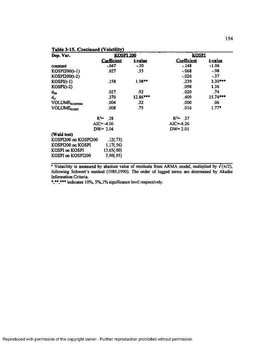
154
Table 3-15. Continued (Volatility)_________________________________Dep. Var. KOSPI 200 KQSPI
Coefficient t-value Coefficient t-valueconstant -.047 -.30 -.148 -1.06KOSPI200(t-l) .027 .35 -.068 -.98KOSPI200(t-2) -.026 -.37KOSPI(t-l) .158 1.98** .239 3.30***KOSPI(t-2) .098 1.36dgjj .027 .92 .020 .74do .370 12.86*** .409 15.74***VOLUMEj-qspeoo .004 .32 .000 .06VOLUMEjjosh .008 .75 .016 1.77*
R*= .28 R ^ .37AIC= -4.06 AIC=-4.26DW= 2.04 DW= 2.01
(Wald test)KOSPI200 on KOSPI200 .12(.73) KOSPI200 on KOSPI 1.17(.56)KOSPI on KOSPI 13.65(.00)KOSPI on KOSPI200 3.90(.05)
* Volatility is measured by absolute value of residuals from ARMA model, multiplied by V(ft/2), following Schwert’s method (1989,1990). The order of lagged terms are determined by Akaike Information Criteria.*,**,*** indicates 10%, 5%,1% significance level respectively.
Reproduced with permission of the copyright owner. Further reproduction prohibited without permission.

155
CHAPTER IV
COMPARISON OF VOLATILITIES BETWEEN
CASH AND FUTURES
4-1. Literature Review
Wood, Mclnish and Ord (1985), Harris (1986), Lockwood and Linn (1990) examine
the volatility features of intraday stock returns and find that the market volatility is high near
the open and close of the trading day, forming the U shape curvature. Finnerty and Park
(1988), Chan, Chan, Karolyi (1991), Ekman (1992), Lee and Linn (1994) and Daigler (1997)
similarly report that stock index futures market also reveals such U shaped intraday volatility
feature. For explanations to this observed patterns of intraday volatility, Kyle (1985) and
Admati and Pfleiderer (1988) suggest that the U shaped volatility patterns result from
interaction between informed traders and (uninformed) liquidity traders, and concentration
of trading by them over the specific time interval within trading hours. Liquidity traders
prefer to trade when the market is thick and thus their trading has little effect on prices,
because they want to minimize adverse selection costs. Informed traders also prefer to trade
when there is more noise trading by liquidity demands since they can effectively hide their
private information and maximize their profit by increasing its informativeness. Therefore, all
strategic traders choose to trade at the same time.46 They argue that non-discretionary
46 Unlike Kyle (1985), Admati and Pfleiderer (1988) differentiate the types of traders by liquidity demands. In their model, non discretionary liquidity traders are traders who must trade a particular number of shares at particular time. Discretionary liquidity traders are traders who also have liquidity demands but who can be strategic in choosing when to execute these trades within a given period of time to minimize the expected cost of their transaction.
Reproduced with permission of the copyright owner. Further reproduction prohibited without permission.

156
liquidity demands increase before and after the exchange is closed since it is difficult or
impossible to trade during that period of time. This in turn induces both discretionary liquidity
trading and informed trading to increase at the open and close. Brock and Kleidon (1992)
insist that the U shaped volatility pattern is a result of the impact of market closure (non
trading hours) on trading preference. They suggest that liquidity demands traders rebalance
their portfolio before and after market closure and this increased liquidity demands create
larger bid-ask spread at the open and close. Market makers have more monopoly power in
setting up the price and tend to increase bid-ask spread when liquidity demand is the highest.
This results is the U shaped patterns in volatility and volume. Daigler (1997) insists that the
U shaped pattern is ubiquitous across the markets so that it is not associated with one type
of market making system or system of determining opening prices.
French and Roll (1986) document that market volatility is also greater during trading
hours than during nontrading periods. They argue that most of return volatility is caused by
private information and that this information only affects prices through the trading of the
informed investors. Stoll and Whaley (1990b) also document that the variance of day time
returns is about five times larger than the overnight returns in NYSE common stocks.
Similarly, Lee and Linn (1994) report that intraday return volatility exceeds overnight return
volatility for both futures return and spot return. In addition, Stoll and Whaley (1990b) find
that the open to open returns has been systematically greater than the close to close returns/7
47 They insist that the information hypothesis can not explain the difference in volatility between the close to close and the open to open returns since they have the same time span. Rather, they maintain that specialists have greater monopoly power at the open than at other times of the day in establishing price at which order imbalances by informed traders and liquidity traders are serviced. Therefore, they try to extract a premium for their
Reproduced with permission of the copyright owner. Further reproduction prohibited without permission.

157
Regarding the volatility comparison between stock and futures markets, Chu and Bubnys
(1990) report that spot market volatilities for both S&P 500 and NYSE indexes are found to
be less than their respective futures price volatilities, concluding that information may flow
faster in the futures markets than in the corresponding stock market, which is consistent with
Ross’s (1989) information-volatility hypothesis.4* Kawaller, Koch and Koch (1990) find that
the mean futures volatility typically exceeds the comparable mean index volatility by five to
ten times. They attribute this inertia in index prices relative to futures price to the infrequent
trading of index stocks, and to the fact that bid-ask bounce is more salient in futures price
than spot index because bid-ask bounce effects tend to be averaged out in cash index price.
The impact of market microstructure effects on volatilities of spot market index or
futures price changes is well reported in the literatures. MacKinlay and Ramaswamy (1988)
and Miller, Muthuswamy and Whaley (1994) show that spot index returns display significantly
positive autocorrelation due to effects of infrequent trading while the autocorrelations of the
fixtures returns are close to zero. Fleming (1994, p.p.33) comments about this asynchronous
trading effect as follows: “The effect of infrequent trading49 is to effectively smooth the
services by setting prices that vary more than the normal bid-ask spread.
4* He argues that in an arbitrage free economy, the volatility of prices is directly related to the rate of information flow to the market.
49 According to Miller, Muthuswamy and Whaley (1994), infrequent trading is divided into non-trading and asynchronous trading. Non-trading means that not every security in the index portfolio trades at the end of price change measurement interval. Asynchronous trading indicates that all securities in the index portfolio trade at least once during each interval but not necessarily at the endpoint. If a stock does not trade at the interval’s endpoint, the observed stock price change in a particular period is attributable not only to true price change innovation in that period but also to true price change innovation in the previous period.
Reproduced with permission of the copyright owner. Further reproduction prohibited without permission.

158
observed (spot) index level. Stocks tend to move together but when the market moves up and
not all o f the stocks in the index have traded, the observed spot index fails to reach the true
height of the market Similarly, when the market falls, the observed index does not reach the
true low. These tendencies provide the usual consequence o f autocorrelated returns and, in
general reduce the variability of the observed (spot) index.” He finds the negative relationship
between trading volume and the size of the first order autocorrelation in the S&P 500 index
returns, and the negative relationship between the extent to which futures volatility exceeds
spot index volatility and the size of the first order autocorrelation in the index returns,
supporting his argument. Fleming (1994) also adds that the comparison of close to close
return volatilities allows a more accurate assessment for true volatility measure between
futures and spot index, because the opening spot index is stale and accordingly, the overnight
(close to open) index return is misleadingly biased to zero.
Lo and MacKinlay (1988) insist that if stock prices are generated by random walks,
the variance of stock returns (log price relatives) increases linearly with the sampling
interval.50 However, variance estimates should be equal regardless of observation intervals
(or intervals aggregated for calculation of variance) once variance estimates are normalized.
They argue that the ratio of variances computed with aggregation value q relative to those
with aggregation value 1 (first differences) is asymptotically normal-distributed and that this
variance ratio statistic is approximately linear combination of the first q-1 autocorrelation
coefficient estimators of the first differences. This means that if autocorrelations at each lag
50 That is, the variance of monthly sampled log price relatives must be 4 times as large as the variance of a weekly sample.
Reproduced with permission of the copyright owner. Further reproduction prohibited without permission.
159
are large and positive, then the variance aggregated for longer intervals is higher than that
aggregated over shorter intervals or vice versa. In empirical tests, they find that variances of
stock returns tend to increase with the observation intervals aggregated for calculation of
variances, which is an evidence against random walk process. They also observe that when
variance ratios are compared over different intervals with different aggregation values,
evidence against random walks for equally weighted index return (small sized stocks) is
stronger than for value weighted index return (large sized stocks) since infrequent trading
induces spurious positive correlation in stock returns and effectively dampens the volatility
of stock returns over short intervals for equally weighted index or portfolios of small sized
stocks.51 In the similar van, Chu and Bubnys (1990) report that the volatility of NYSE index
including smaller stocks is lower than the S&P 500 index volatility. Board and Sutcliffe
(1995) also support their findings in that extra futures volatility over the FT-SE 100 index
return are found to decrease with the length of measurement interval (input frequency). As
MacKinlay and Ramaswamy (1988) insist that the problem of non-synchronous data in the
index series is mitigated by employing longer measurement interval, they find that futures
return volatility is greater than the corresponding spot volatility by 82% in hourly returns
while volatility for futures is greater than that for spot index by 18% in weekly return.
Alternatively, Roll (1984) insists that the bid-ask bounce induces the negative first
order autocorrelation in observed price change of an individual stock. Lo and MacKinlay
(1988) find that unlike stock index returns or returns on portfolio, the first order
51They estimated that the 1st order autocorrelation for a portfolio of small sized NYSE- AMEX stocks is .42 while that for largest stocks is mere . 14.
Reproduced with permission of the copyright owner. Further reproduction prohibited without permission.

160
autocorrelation of an individual stock return is small, but negative regardless of aggregation
intervals. Miller, Muthuswamy and Whaley (1994) maintain that the bid-ask bounce shows
up more strongly in futures return than spot return, because the spot index is an average of
prices across stocks at given point in time and the trading by some stocks traded most
recently at bid prices is offset by other stocks trading most recently at ask levels while futures
contract is a single traded security. They add that positive first order autocorrelation in the
observed spot index return may underestimate the true volatility for spot index return while
negative first order autocorrelation in futures return may possibly overestimate the true
volatility for futures return.52 However, they observe that the effect of bid-ask spread in
52 The model which accounts for infrequent trading in the spot index level can be expressed by 1st order autoregressive ( AR(1)) process as follows.
st° = 4*,!, + ( i - (j> )St
where St = the true index level change, St° = the observed index level change <J) = the degree of trading infrequency or 1st order autocorrelation ( 0 i <f> i 1 ) According to this model, the variance of observed changes in the stock index level is,
•i.- i -<!> 1 + <J>
On the other hand, the model which accounts for bid-ask bounce in futures price can be expressed by 1st order moving average ( MA(1)) process as follows.
Ft° = Ft + 0Fm
where F, = true futures price change, F,° = the observed futures price change 6 = the bid-ask bounce parameter or 1st order autocorrelation in futures price change
( - 1< 0 < 0 )According to this model, the variance of observed changes in futures price is,
Reproduced with permission of the copyright owner. Further reproduction prohibited without permission.

161
futures price changes is trivial and can be ignored in the empirical test. Similarly, Harris,
Sofianos and Shapiro (1994) record that variance of one minute (five minute) futures return
is 4.6 (1.9) times larger than that of index return for S&P 500 index. Moreover, they also
find that ratios of five minute return variances to one minute return variances are 12.5 for
S&P 500 index and 5 for its corresponding nearby futures contract, confirming that futures
returns are largely uncorrelated while S&P 500 index returns are positively correlated. They
argue that futures market seems to discover index values faster than the cash index market
since the absence of significant negative correlation in the futures returns suggests that
futures’ high volatility is not due to short-term liquidity problems, i.e., bid-ask bounce.
Previous studies suggest that smoothing effects from infrequent trading or bid-ask
bounce are not sources of fundamental volatility, but either a statistical illusion (Miller,et al.
1994) or an artifact of the process by which liquidity demands are routinely satisfied (Harris,
et al.1994). Therefore, before any comparison is made regarding the volatilities between
futures price and corresponding spot index, these spurious microstructural effects are sifted
out from fundamental volatilities by pre-whitening procedures and residual volatilities
between two assets should be compared to determine whether futures market really adjust
o\0 = ( 1 + 02 WF
Reproduced with permission of the copyright owner. Further reproduction prohibited without permission.

1 6 2
faster than spot market to the new information in the market.
Even though problems of infrequent trading are not explicitly accounted for, Brenner,
Subrahmanyam and Uno (1989,1990) observe in the Japanese market, futures market are
more volatile than respective stock market in the early introduction period (September 1986
to June 1988), but in the later periods (December 1988 to September 1989), the volatilities
of the futures contracts are lower than the volatility of the underlying index. Using five minute
transaction data, Lim (1992) reports no apparent positive or negative autocorrelation in either
returns of Nikkei average fixtures contract or respective cash index, concluding that staleness
of spot prices is not a significant problem beyond five minutes and that Nikkei spot market
is at least weakly efficient with respect to information on futures prices at SIMEX. Over his
sample period (1988.6-9), he also observes that there are considerably many trading days
when futures price is less volatile.
As for the U.K. futures market (FTSE-100 futures contract), Yadav and Pope (1990)
report that average intraday volatility of price changes (based upon daily high and low prices)
in the fixtures market is significantly higher than in the cash market.They also document, even
though less apparent, that interday volatility based upon open to open or close to close price
changes is higher for futures market than for cash market.
In addition to the microstructural effect explanation for extra volatility of fixtures
contract over spot index, Chan, Chan and Karolyi (1991) suggest that bilateral volatility
spillover between fixtures and cash index or between futures and individual stocks are not
likely driven only by such microstructural effect as infrequent trading. They argue that if the
index futures market plays a greater role in reflecting the market-wide information, the
Reproduced with permission of the copyright owner. Further reproduction prohibited without permission.

163
volatility of index futures returns are expected to be greater than volatility in the stock market
when the markets are driven by that information. Kawaller, Koch and Koch (1990) also
indicate that futures price may be more speedy in reflecting information and thus more volatile
than spot index, because market participants can take position in index futures quickly with
low transaction costs when new information becomes available.
With respect to the expiration date effect on the stock market volatility, Stoll and
Whaley (1987) report that the volatility of S&P 500 index is significantly high with the stock
market tending to fall along with increase in volume when index futures and index options
expire together. However, they also report that when only index futures expires53, volatility
of the stock market does not increase abnormally compared to those on the non-expiration
days. Moreover, they present evidence that volatility increase on the expiration day is
associated only with stocks included in the S&P 500 index, not with stocks that are not part
of the stock index since unwinding of arbitrage position at expiration affects only those stocks
in the S&P 500 index. They also find that the expiration effect on the stock market is
concentrated during a very short period of time, within the last three hours or sometimes last
15 minutes of trading. Similarly, Edwards (1988) reports that volatility shock on spot index
53 Prior to June 15, 1984, the last trading day for S&P 500 index futures contract was the third Thursday of the delivery month and the last marking to market was based on the last spot S&P 500 index value on that day. From June 15,1984 until March 20,1987, the last trading day was the third Friday of the delivery month. For this period, the effect of triple witching hours (stock index futures, stock index option and individual stock option expire on the same day)on abrupt stock market volatility emerged as a great concern for market regulators.Therefore, the CME changed the final settlement procedures for its S&P 500 futures contract such that trading of futures contract ceases at the close on Thursday and all open positions are marked to market for the last time based on a special opening quotation for the S&P 500 index on the third Friday of the delivery month.
Reproduced with permission of the copyright owner. Further reproduction prohibited without permission.
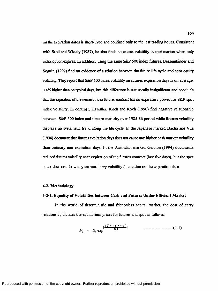
164
on the expiration dates is short-lived and confined only to the last trading hours. Consistent
with Stoll and Whaely (1987), he also finds no excess volatility in spot market when only
index option expires. In addition, using the same S&P 500 index futures, Bessembinder and
Seguin (1992) find no evidence of a relation between the future life cycle and spot equity
volatility. They report that S&P 500 index volatility on futures expiration days is on average,
. 14% higher than on typical days, but this difference is statistically insignificant and conclude
that the expiration of the nearest index futures contract has no expiratory power for S&P spot
index volatility. In contrast, Kawaller, Koch and Koch (1990) find negative relationship
between S&P 500 index and time to maturity over 1985-86 period while futures volatility
displays no systematic trend along the life cycle. In the Japanese market, Bacha and Vila
(1994) document that futures expiration days does not cause any higher cash market volatility
than ordinary non expiration days. In the Australian market, Gannon (1994) documents
reduced futures volatility near expiration of the futures contract (last five days), but the spot
index does not show any extraordinary volatility fluctuation on the expiration date.
4-2. Methodology
4-2-1. Equality of Volatilities between Cash and Futures Under Efficient Market
In the world of deterministic and frictionless capital market, the cost of carry
relationship dictates the equilibrium prices for futures and spot as follows.
r ( T - t X r - d )
F, = S, exp 1 (4-D
Reproduced with permission of the copyright owner. Further reproduction prohibited without permission.

165
where F, = current futures price at time t
St = current spot price at time t
T = expiration date
t = current date
r = annualized interest rate ( non stochastic )
d = annualized dividend yield ( non stochastic )
If we take the natural logarithm for both sides of equation, then we get
ta* = |„s- - ^ T - t X r - d ) ---------------------------------- ( 4 . 2 )
365
Let Rfl = ln[ Ft /F « ] and R„ = ln[ St /S « l be continuous compounding futures return and
spot return respectively. Then we have
Rft = R* + ( r - d )/ 365 -------------------------------- (4-3)
and accordingly
Var(Rft) = Var ( R* ) ---------------------------------- (4-4)
( v Var [ (r-d)/365 ] = 0 , C o v [ R lt, (r-d)/365] =0 )
This means that the return volatility for the futures contract equals the return volatility for the
spot index when we assume that capital markets are frictionless and deterministic.
Reproduced with permission of the copyright owner. Further reproduction prohibited without permission.

166
4-2-2. Measurement of Price Volatilities Using Historical Data
First, we investigate price volatilities for cash and futures markets using historical
daily price data The classical estimator of price volatility employs only the closing price from
each holding period.54 Parkinson (1980) develops the extreme value method for estimating
return volatility using the high and low prices and insists that his method generates at least
five times more efficient volatility estimator than the classical method. Based upon the
historical opening, high, low and closing price data, Garman and Klass (1980) further extend
Parkinson’s (1980) method and elaborate at least seven times more efficient volatility
estimator than that relied upon the only daily closing data. Although both Parkinson and
Garman-Klass’ volatility estimators are likely to be downward biased for stocks with low
trading volumes, Wiggins (1992) documents that these estimators are only slightly downward
biased and are significantly more efficient than the close to close estimator for assets with high
trading volumes such as S&P 500 futures. Since estimators incorporating more information
about stock price change over an interval are found to be more efficient than those using less
information, we first compare the price volatility between cash and futures markets using
Garman and Klass’ (1980) volatility estimation method.
Garman and Klass volatility estimator (hereinafter G-K estimator) can be measured
in two ways and calculated by the following formulas :
54 The classical volatility estimator can be measured as square o f natural logarithm of the closing price ratio over two periods.
Reproduced with permission of the copyright owner. Further reproduction prohibited without permission.

167
02GKl = 0.511( u - d f - 0.019[ c(u + d) - 2ud ] - 0.383c2---------- (4-5)
In (0 . / C J2 = 0.12 — — l- ---------- — + 0.88
/(4-6)
where C0 = previous closing price.
0 1 = today’s opening price.
u = natural logarithm of the ratio o f today’s high to today’s opening price,
d = natural logarithm of the ratio of today’s low to today’s opening price,
c = natural logarithm of the ratio of today’s closing to today’s opening price,
f = fraction of non-trading hours in a single day when the time from yesterday’s
market close to the today’s market close is assumed to be one.
In Korean market, f « .7708.
The first measure ( o2 ) assumes that trading is made continuously around the clock
and the second one ( o2 ) accounts for the existence of non-trading hours, and hence takes
into account the fret that the today’s opening price may differ from the previous closing price.
4-2-3.Tests for the Homogeneity of Variances
The statistical power of usual F test which compares the sample variances of two
groups (F = Sj2 / S*2 ) relies on the assumption that the underlying populations are from
Gaussian normal distribution. That is, when the underlying distribution are non-normal, F test
loses its power. Since we already know that the return distributions of futures and spot index
Reproduced with permission of the copyright owner. Further reproduction prohibited without permission.

168
take on non-normal distribution, we have to apply other statistical tests to our sample that are
robust to non-normality. Brown-Forsythe’s (1974) modified Levene test is one of those that
is used to test for the homogeneity of variances between two samples and robust to the
departures from normality.55
Suppose we have i groups ( i = 1,2,....g ) and j observations ( j = 1,2,......,N;) for each
i group and sample values ( Xg) can be expressed as sum of the population mean ( g ) for
each group and error term (6j), that is, Xg = + e*,-. The means are neither known
nor assumed equal and the ey are independent and similarly distributed with zero mean and
possibly unequal variances. Then Brown-Forsythe’s (1974) modified Levene test statistic56
is as follows :
£ n, ( Z t - z ? K g - 1 )w = — -------------------
* N‘ - ,E E/=1 / = I 1=1
N, g
E _ E EZy ~ I Xy ~ %i I where X. is median o f i group, Zt = —------, Z = ———------
" ± » ,i=i
55 Brown-Forsythe modified Levene test (1974) is used widely in empirical finance research such as Lockwood and Linn (1990), Lee and Linn (1994), Chang, Jain and Locke (1995) and Crain and Lee (1996).
56 Levene test (1960) uses the sample mean for each group instead of the median in Brown-Forsythe’s modification in calculating Z,j statistic.
■ t ( N, - 1 ) (4-7)
Reproduced with permission of the copyright owner. Further reproduction prohibited without permission.
169
With the null hypothesis o f equal variances among groups, W statistic is compared with the
critical value of F distribution with degree of freedom of (g-l)for numerator and (2 [N{ - 1])
for denominator. In our study, the number of groups becomes two (g =2) for futures and spot
index and the number of observations (Nj) for each group becomes 2715 for 10 minute
intraday returns, 132 for volatilities of open to open, close to close, close to open, 112 for
open to close37, noon to close (more precisely speaking, from the beginning of afternoon
session to its close) returns and session break returns and 135 for volatilities of open to noon
(more precisely from open to the end of the morning session) returns.
4-3. Empirical Results Concerning Comparison of Volatilities between Cash and Futures Market
4-3-1. Intraday Patterns of Volatilities
As is shown in Table 4-1 and Chart 4-1, The intraday volatility pattern of the Korean
stock market (including index futures market) shows a similar U curvature when the standard
deviation of the 10 minute returns is used as volatility measure just as documented in other
country markets. The U type pattern is more conspicuous in the spot markets than in index
futures market. Index futures show more fluctuation during the trading hours than the spot
market. For both futures and spot markets, the 10 minute returns tend to rise around the end
of the morning session as well as near the end of the afternoon session. Therefore, the Korean
stock market displays double U curvatures over the whole trading hours, one in the morning
57 There is only a morning session on Saturday and the open to close returns on Saturday are included in the open to noon returns in our study.
Reproduced with permission of the copyright owner. Further reproduction prohibited without permission.

170
session and the other in the afternoon session. Daigler (1997) reports the similar double U
shapes o f intraday volatility structure in Treasury bond futures trading. In Table 4-2,
volatilities in the stock and futures markets are compared according to the time intervals.
Consistent with previous studies in other countries’ markets, the overnight returns during
non-trading hours shows less volatility than day time returns (open to close) during trading
hours. Almost similar to the studies in the U.S. market by Stoll and Whaley (1990b), the
volatility (variance) of trading hour returns is about 4-6 times larger than that of non-trading
hour return in the Korean securities market. As the theory dictates, the positive
autocorrelation resulting from asynchronous trading in the stock index seems to dampen the
volatilities in the spot index, making futures more volatile than KOSPI200, and subsequently
KOSPI 200's volatility greater than that for KOSPI. Also consistent with Stoll and Whaley
study (1990b), the variance of open to open returns is greater by 30 - 40 % than that of close
to close returns, whose difference is somewhat larger than the case in the U.S.58 In panel 3
of Table 4-2, standard deviation of session break return is almost as much as that of 10 minute
intraday returns during trading hours. Since the time span for session break returns is 9 times
longs' than that for 10 minute returns, this result also supports that volatility in non trading
hours is lower than the comparable volatility in trading hours.
In Table 4-3, the first autocorrelation coefficients of returns for various time horizons
are presented to examine to what extent return reversal tend to take place for each of the
58 Stoll and Whaley (1990b) report the variance of open to open returns on NYSE common stocks is 13% greater than that of close to close returns. They argue that the greater volatility of open to open returns reflects the specialist’s implied cost of supplying immediacy upon price pressure by traders at the open.
Reproduced with permission of the copyright owner. Further reproduction prohibited without permission.

171
return series. Stoll and Whaley (1990b) report that serial correlation in open to open returns
is more consistently negative and larger in magnitude than close to close returns, suggesting
that open to open returns are more likely to be reversed and accordingly, more volatile than
close to close return. Over the June contract period, 1st order autocorrelation o f both open
to open and close to close returns are negative, but the magnitude is larger for open to open
than close to close returns. For September contract periods, the autocorrelations are almost
close to zero for open to open returns except for futures with negative autocorrelation and
significantly positive for all close to close returns. Over the December contract periods, open
to open returns show positive autocorrelation and close to close returns display close to zero
serial correlation. Therefore, daily open to open return tend to reverse itself more frequently
(leading to higher volatility) than the corresponding close to close return until September
contract period, but over December period this tendency does not hold. It is observable that
futures contract returns have strong tendencies to reverse relative to its respective spot index
returns across the measurement intervals. Throughout the whole sample period, daily futures
returns have larger negative autocorrelation in magnitude than spot index returns during June
contract period and less positive or close to zero autocorrelation than the corresponding spot
index returns over the September and December contract periods. Negative autocorrelation
(or mean reversal) of daily futures returns indicates that futures tend to be more volatile
(fluctuate more wildly) than spot indexes. This fact in turn supports that information flows
faster in the futures market than in the spot market and that futures market provides an
important price discovery function to the investors.
As a whole, daily returns in the Korean stock market and index futures market have
Reproduced with permission of the copyright owner. Further reproduction prohibited without permission.

172
strong tendencies to reverse over the June contract periods where futures contract price
moves relatively within its cost of carry boundary, but as the stock market gets depressed
after September contract period, consistently negative daily market returns make the 1st
order serial correlations positive. Chan and Chung (1993) document a negative relationship
between mispricing of futures contract and market volatility. Consistent with their findings,
market inertia results in persistence of returns rather than mean reversal. Due to lack of
arbitrages, reduced volatility across the markets consequently brings about a persistent
mispricing of futures contract over these two periods. In Table 4-4, correlation between
daytime (open to close) returns in a previous day seems to be consistently positively
correlated with overnight returns for the next day. This indicates that the market direction
shown in trading hours in one day tends to persist and is not likely reversed during non
trading hours. In contrast, overnight returns are more likely to be reversed during trading
hours and at least not correlated with day time returns. Stoll and Whaley (1990b) observe this
phenomenon in the U.S. market and this result is consistent with French and Roll’s (1986)
argument that information arrives more during trading hours than during non trading hours.
It is also observed in Table 4-4 that correlation between overnight and daytime futures returns
are on average less positive or more negative than those for the spot indexes. This also
supports a strong tendency of futures price for mean reversal.
4-3-2. Comparison of Volatility using Extreme Value Method
In Table 4-5, we compare volatilities among stock indexes and futures contract using
the Garman Klass (1980, hereinafter G-K) price volatility estimators. In each return series,
Reproduced with permission of the copyright owner. Further reproduction prohibited without permission.

173
two measures of G-K volatility estimators are presented. One assumes that trading is
continuously executed and the other accounts for existence of the non-trading hours. Over
the whole contract periods and by either of two measures of G-K price volatility estimators,
futures contract shows the greatest volatility of three return series. KOSPI 200 displays the
second largest volatility and KOSPI is the least volatile. This result is consistent with previous
studies since KOSPI and KOSPI 200 tend to have positive serial correlation due to infrequent
trading of component stocks or reporting lag while futures does not. In addition, infrequent
trading is more severe among small sized stocks that are more included in KOSPI rather than
in KOSPI 200. When volatility comparison is made between expiration day week and non-
expiration day weeks, two stock indexes are slightly more volatile during the expiration day
week than non-expiration day weeks but neither of them is significantly different. In contrast,
futures market tends to be more tranquil in expiration day week than non-expiration day
weeks. During expiration day week, futures market’ volatility is even lower than those of
stock indexes. Tauchen and Pitts (1983) insist that price volatility increases with the extent
to which traders disagree with each other in relation to the market equilibrium price. Kyle
(1985) also maintains that price volatility is determined by the amount of noise (liquidity
demand) trading. He argues that the market depth is proportional to the amount of liquidity
trading and inversely proportional to informed trading. These suggest that as the futures
contract is about to expire, the amount of noise trading relative to information based trading
tends to increase since the market is more likely driven by liquidity demand trades according
to unwinding process of the existing positions. Discrepancy regarding fair futures price also
tends to be converged and these effects result in reduction of volatility of futures price. In
Reproduced with permission of the copyright owner. Further reproduction prohibited without permission.
174
addition, slight increase in spot volatility may indicate the effect of arbitrage unwinding on
spot market.
4-3-3. Test Results of Homogeneity of Variances between Cash and Futures Markets
In Table 4-6, results of standard F test and Brown-Forsythe’s (1974) modified Levene
F test (hereinafter B-F-L test) on homogeneity of variance are presented. Since most of
returns have non-normal distribution as seen in Chapter HI, the B-F-L F test can be more
robust than the standard F test to examine homogeneity of variance between futures and cash
market. Generally, results indicate that on average, futures returns are consistently more
volatile than stock indexes, especially during trading hours. In non-trading hours, futures’
volatility is not significantly greater than stock indexes, signaling that futures tend to reflect
more rapidly than spot market only when new information reaches the market. Consistent
with earlier studies (for example, MacKinlay and Ramaswamy 1988 ; Board and Sutcliffe
1995 ; Harris, Sofianos and Shapiro 1994), asynchronous data in the index is mitigated by
employing longer measurement interval and futures’extra volatility over spot decreases with
sample interval (e.g., compare standard F test ratio in 10 minute interval with those in other
measurement interval).
In Table 4-7, the first order autocorrelation present in each return series is corrected
by revising raw return data with AR(1) specification used in Miller, Muthuswamy and
Whaley (1994). Before applying AR(1) modification, the first differenced original price series
of KOSPI, KOSPI 200 and the nearby futures have significantly high positive autocorrelation
amounting to .35, .36 and .12. After the first order autoregressive modification, their first
Reproduced with permission of the copyright owner. Further reproduction prohibited without permission.

175
order autocorrelation coefficients are reduced to less than .01 in absolute value.59 Although
we arbitrarily revise actual raw prices, results are very similar to the cases when actual raw
returns are used. Futures again tend to be more volatile than stock indexes and KOSPI 200
tends to be more volatile than KOSPI.60 Therefore, infrequent trading alone can not explain
the extra volatility of futures over stock indexes. Information arrives constantly in the
markets, more during trading hours than during non-trading hours, and traders in the futures
market seem to respond to that information faster due to various reasons such as lower
transaction and adverse selection costs.
4-3-4. Analyses of Volatility and Trading Volumes around Futures Expiration Dates
In Table 4-8, comparison is made using raw returns between volatilities in expiration
week and non-expiration week. For all return series, the volatilities of non-expiration week
are slightly higher than those for expiration week. Except for 10 minute intraday returns for
KOSPI 200 and futures, and overnight returns for futures, however, the B-F-L test for
homogeneity of variance can not reject the null hypothesis of equal variance between
expiration week and non-expiration week. On average, futures tend to show less volatility in
expiration week than in non-expiration week compared to the stock index. This is consistent
59 As Miller, Muthuswamy and Whaley (1994) put it, the AR(1) model is too simple and insufficient to get rid of all spurious positive autocorrelation embedded in stock indexes. However, an attempt to at least correct for such autocorrelation would be worthwhile.
60 However, there is one exception in this result. For overnight returns after AR(1) modification, it turns out that volatilities for stock indexes tend to more volatile than futures. However, it is not unexpected since the standard deviation of futures is the closest to those for stock indexes in case of the close to open returns, i.e., during non-trading hours. This may be another spurious side effect the AR(1) modification might bring in.
Reproduced with permission of the copyright owner. Further reproduction prohibited without permission.

176
with results obtained from G-K price volatility estimators. Generally, in the Korean market,
there is no tendency for stock market volatility to rise around the expiration date, which is
generally consistent with what has been documented in other countries.
Table 4-9 displays the comparison of trading volumes in the spot and futures markets,
particularly changes in the volume o f respective market between expiration week and non
expiration weeks. Stoll and Whaley (1987) report that NYSE stock trading volume is
substantially higher than normal when index futures and index options expire on the same day.
Over the period of 1984-85, they find that spot trading volume increases by 13% per week
basis, 17% per daily basis and 95% in the last trading hour, suggesting that expiration effect
on the spot volume is confined rather to the last trading hours. Bessembinder, Chan and
Seguin (1996) document that over 1982-91 period, futures trading volumes gradually
increased as expiration date approaches but on the expiration date, they are significantly
reduced. On the other hand, increase in NYSE volumes is confined only to the expiration date
of futures contract. They use changes in futures open interest as a proxy for changes in the
dispersion of traders’ belief and find that trading volumes in the both the spot and futures
markets rises with increase in open interest (divergence of investors’ opinions) while decrease
in open interest (convergence of investors’ opinion) is less associated with any discernible
effect on the volumes in each market. They notice that expiration of futures contract reduces
the number of open interest without triggering volume increase (on the contrary, a significant
decline in futures volume) and interpret this as a result of evidence of convergence in traders’
opinion.
As for trading volumes in the June contract period in Table 4-9, both spot and futures
Reproduced with permission of the copyright owner. Further reproduction prohibited without permission.

177
volumes in the Korean market tend to drop in the expiration week (June 10-13) relative to
non-expiration weeks. On expiration date (June 13), both trading volumes in futures and spot
market decrease by 59% and 39% respectively. Over the September contract period, there
is little difference in both futures and spot trading volumes in between expiration week and
non-expiration weeks. Due to the depressed market condition, significant drop in spot trading
volume is observed. On the expiration date of September contract (September 12), volume
in futures contract is significantly reduced (- 41%) while spot volume increases by 13.8%.
Reduced trading volumes in futures contract around the expiration dates are consistent with
reduced volatility of futures contract around the expiration date. They are also generally
consistent with Bessembinder, Chan and Seguin’s (1996) convergence of traders’ opinion
hypothesis. Absence of systematic increase in spot trading volumes around the expiration
dates of futures contract is also consistent with a result that spot index does not show any
extreme volatility around the expiration dates. MacKinlay and Ramaswamy (1988), Merrick
(1989),Yadav and Pope (1990) insist that early unwinding or rolling over makes expiration
day effect unlikely. Merrick (1989) argue that simple net mispricing days rule61 has a poor
prediction ability to forecast cash index price changes on the expiration date because
arbitrageurs’ early closing out or rolling over existing futures contracts mitigates unwinding
force on the expiration date. He reports that about 57% of expiration dates in the sample
61 Simple net mispricing rule of thumb asserts that a contract which has been underpriced (overpriced) more days than it has been underpriced (overpriced) will be associated with an accumulation of net short (net long) cash stock positions by arbitrageurs. Such short (long) cash position must be covered by stock purchase (sales) at expiration. Thus net underpricing (overpricing) would predict a stock price rise (drop) at expiration (see Merrick 1989, p.p. 109).
Reproduced with permission of the copyright owner. Further reproduction prohibited without permission.

178
period (1982.6- 1986.3) are presumed not to be associated with expiration day unwinding.
MacKinlay and Ramaswamy (1988) also suggest that early unwinding opportunity makes
expiration day predictions based on the identification of mispricing difficult. In Korea, risk
averse investors (especially subject to institutionally imposed risk exposure) tend to behave
more like day traders or scalpers rather than position traders. They are likely to unwind their
position whenever their profits exceed their expected returns or their losses exceed their
maximum allowed losses.62 Table 4-10 displays the 10 minute intraday returns and variances
as well as close to close interday returns of spot index and futures contract on the expiration
dates (June 13th and September 12th). Consistent with previous results, futures and spot
index do not reveal high volatility at the expiration. Although spot index shows somewhat
greater price fluctuation on the expiration date of June contract than does it over the non-
expiration weekdays, its volatility on the expiration date of September contract is lower than
those for ordinary non-expiration weekdays. For both expiration dates, futures’ volatility
tends to diminish as evidenced in the previous results (see Table 4-8). Expiration day returns
for KOSPI 200 are on average negative except for close to close return on June contract
expiration date. Frequent underpricing of futures contract over the September contract period
is expected to cause price run up in spot index on expiration date if reverse transactions by
arbitrageurs’ unwinding were heavy in the spot market. However, consistent with results
obtained in the Chapter II, insufficient arbitrage transactions do not trigger either stock
62 In its report on June 4,1996, Korea Economic Daily says that most of Korean investors in futures market are engaged more heavily in speculative trading rather than hedge trading. It adds that about 73% of futures open positions are closed within a day in the Korean market.
Reproduced with permission of the copyright owner. Further reproduction prohibited without permission.
179
purchases by reverse transactions or price rise in the spot index on the expiration date. This
result supports Merrick’s (1989) findings and suggests that in the face o f sluggish stock
market condition, Korean futures market has been mainly driven by speculative traders rather
than hedgers or arbitrageurs, and early unwinding by traders weakens the impact o f expiration
on spot market volatility. In addition, the absence of volume increase around expiration dates
is consistent with the argument that investors’early unwinding practice in the Korean futures
market makes the effect of futures’expiration on volatility and volume diminished. Chart 4-2
graphically shows the changes in the trading volumes and open interest in the Korean market
over the sample period.
Table 4-11 shows the ratio of open interest change to daily trading volume of futures
contract for each contract period. Chart 4-3 displays the trend of this ratio graphically. Over
the whole sample period, daily trading volume in futures on average brings about mere 1-2%
increase in open interest for non-expiration weeks. This fact indicates that the transactions
(volumes) resulting from traders’ early unwindings take a significant portion of the total
trading volumes. Convergence of traders’ opinion (downward revision) toward the expected
future spot price triggers frequent early closing of the established futures positions. Open
interest increase relative to daily futures volume have the least average (median) value during
September contract period. This result is also consistent with huge mispricing of futures
contract over September contract period shown in the chapter one. Due to lack of sufficient
data, however, it is premature to draw any conclusion on patterns of changes in trading
volumes around the expiration dates.
Reproduced with permission of the copyright owner. Further reproduction prohibited without permission.

I S O
4-4. Conclusion
In this chapter, we compare volatilities between cash and future markets in the early
introduction period of index futures. We examine the volatility of each market with the
extreme value method proposed by Garman and Klass (1980) and test the homogeneity of
variance using Brown- Forsythe (1974) modified Levene F statistics. Consistent with earlier
studies, futures market on average tend to be more volatile than cash market over the whole
sample period. Even after correcting for positive autocorrelation in the stock index, the results
basically are not changed. If price variability reflects the rate of information arrival as
proposed by Ross (1989), these results suggest that futures adjusts more quickly than spot
to the new information occurred in the marketplace, which is consistent with outcomes
obtained in Chapter m. We also investigate whether the degree of volatility changes for each
market around the expiration of futures contract. Also consistent with earlier research, spot
market does not show any extreme volatility around the expiration date of futures contract.
On the other hand, futures tend to be more tranquil around the expiration, which is consistent
with what is predicted in Tauchen and Pitts (1983) and Kyle (1985).
The analysis of trading volume in both spot and futures markets also supports our
results regarding volatility changes around the futures expiration. Investors’ early unwinding
of the existing futures contracts before expiration is presumed to make expiration day effect
unlikely.
Reproduced with permission of the copyright owner. Further reproduction prohibited without permission.

181
Table 4-1.Standard Deviations of the Intraday 10 Minute Percentage Returns for the KOSPI 200 Cash Index, Futures Contract and for KOSPI Composite Index for the Periods of May 3,1996 - October 16, 1996_____________________________________
TIME KQSPI200 Futures KOSPI
9:50 0.199215 0.208427 0.18180910:00 0.168342 0.179391 0.15723310:10 0.164955 0.199382 0.15633710:20 0.188384 0.204109 0.17184910:30 0.161727 0.180075 0.15279410:40 0.162040 0.198563 0.14970210:50 0.137706 0.187046 0.13196311:00 0.142112 0.164083 0.13113811:10 0.148915 0.191097 0.13652411:20 0.165844 0.256434 0.15931711:30 0.145799 0.178072 0.12796513:10* 0.175791 0.211826 0.16702813:20 0.140946 0.222206 0.13310613:30 0.139234 0.170575 0.12905713:40 0.139376 0.225442 0.13083013:50 0.133381 0.181561 0.12898814:00 0.120994 0.216294 0.10515814:10 0.134987 0.219470 0.12770214:20 0.129953 0.240064 0.12568314:30 0.155016 0.252268 0.15102614:40 0.170542 0.262816 0.17516114:50 0.177926 0.274225 0.17006015:00 0.138935 0.164182 0.032038
* Standard deviation in this time span covers standard deviation during session break ( 1 hours and 30 minutes), not standard deviation of 10 minute intraday return.
Reproduced with permission of the copyright owner. Further reproduction prohibited without permission.

Reproduced
with perm
ission of the
copyright ow
ner. Further
reproduction prohibited
without
permission.
Chart 4-1. Patterns of intraday volatilities
0.3
0 2 5
0.2
sRq 0.15CO
0.05
oinai
8oo oM 8 2 8 8 9 8 2 8 8 9 8 8
if if if if if if lijCO
Time
KOSPI200
Future
KOSPI
ooto

183
Table 4-2. Comparison of Volatilities according to Trading Hours*Day Time(A)
(Open to Close) STD(%)k
Overnight(B)( Close to Open)
STD(%)
Ratio<A/B)
KOSPI 200 1.0482 .4932 2.13KOSPI .9497 .4815 1.97Futures 1.2088 .4963 2.43
Open to Open Close to Close Ratio (A/B)STD(%) STD(%)_JA *_____________________ (5 )__
KOSPI 200 1.2667 1.1135 1.14KOSPI 1.2111 1.0480 1.16Futures 1.4178 1.1962 1.19
Session Break 10 minute Ratio (A/B)STD(%) STD(%)_ & ) _________________(B)__
KOSPI 200 .1758 .1573 1.12KOSPI .1670 .1455 1.15Futures .2118 .2106 1.01* Returns on the expiration dates are excluded for comparison purpose.b If the open to close returns on Saturday is included in calculation, the standard deviations of day time returns for KOSPI 200, KOSPI and futures are .9927%, .8982% and 1.1362% respectively and the ratios of day time returns to overnight returns are 2.01,1.86 and 2.29 respectively.
Table 4-3.The First Order Autocorrelation of Returns according to Trading Hours1. Open to Close
JuDfi September DecemberKOSPI 200 -.263 .156 -.005KOSPI -.193 .144 .019Futures -.198 -.014 .001
2. Close to OpenKOSPI 200 -.150 -.122 .475KOSPI -.134 -.103 .317Futures -.139 -.196 .139
3. Open to OpenKOSPI 200 -.227 .049 .192KOSPI -.162 .078 .164Futures -.188 -.143 .162
4. Close to CloseKOSPI 200 -.178 .236 .093KOSPI -.094 .296 .073Futures -.108 .162 -.044
Reproduced with permission of the copyright owner. Further reproduction prohibited without permission.

184
Table 4-4.Correlation between Open to Cose (Daytime) and Close to Open(Overnight) Returns1. Correlation between Daytime at t-1 and Overnight at t
June September December
KOSPI 200 .489 .446 .418KOSPI .492 .516 .409Futures .301 .521 .273
2. Correlation between Overnight t and Daytime at t
June September December
KOSPI 200 -.093 .155 .037KOSPI -.100 .180 .029Futures .064 -.137 -.002
Table 4-5. Comparison of the Average Garman-KJass ( G-K) Price Volatility Estimators* among KOSPI Stock Index, KOSPI 200 Index and Index Futures._____
KOSPI KOSPI 200 FuturesG-K I G-K 2 G-K I G-K 2 G-K 1 G-K 2
June 5.15E-05 .000201 7.16E-05 .000272 7.83E-05 .000304
September 4.55E-05 .000177 5.83E-05 .000224 .000110 .000426
December 5.90E-05 .000232 9.91E-05 .000382 .000127 .000498
ExpirationbWeek 5.15E-05 .000198 7.19E-05 .000276 4.28E-05 .000165
Non-Expiration Week 4.94E-05 .000193 6.90E-05 .000265 .000109 .000425
Total 4.95E-05 .000193 6.92E-05 .000265 .000105 .000409*G-K1 estimator is based on the continuous trading around the clock and G-K 2 estimator accounts for the existence of non trading periods.b Expiration week sample covers total eight days, June 10-13 and September 9-12,1996.
Reproduced with permission of the copyright owner. Further reproduction prohibited without permission.

185
Table 4-6. Results of Test for Homogeneity of Variances with Raw Returns*(1) 10 minute intraday returns ( N=2715)
KOSPI 200FutureKOSPI
s i p m.1573.2106.1455
KOSPI 200 vs Future KOSPI 200 vs KOSPI
Future vs KOSPI
(2) Open to Open returns ( N=132)
STD (a/-KOSPI 200 1.2667 KOSPI 200 vs FuturesFutures 1.4178 KOSPI 200 vs KOSPIKOSPI 1.2111 Futures vs KOSPI
(3) Open to Close returns ( N=112)b
s n a mKOSPI 200 1.0482 KOSPI 200 vs FuturesFutures 1.2088 KOSPI 200 vs KOSPIKOSPI .9497 Futures vs KOSPI
(4) Close to Open returns ( N=132)
KOSPI 200FuturesKOSPI
STP-(%)-.4932.4963.4815
KOSPI 200 vs Futures KOSPI 200 vs KOSPI
Futures vs KOSPI
(5) Close to Close returns ( N=132)
KOSPI 200FuturesKOSPI
STD m . 1.1135 1.1962 1.0480
KOSPI 200 vs Futures KOSPI 200 vs KOSPI
Futures vs KOSPI
(6) Session Break returns ( N=112)
KOSPI 200FuturesKOSPI
STD.(%X.1758.2118.1670
KOSPI 200 vs Futures KOSPI 200 vs KOSPI
Futures vs KOSPI
68.60*** 1.79***5.89*** 1.17***
82.93*** 2.09***
B-F-L Revised F test Standard F test.69 1.26*.06 1.09
1.15 1.37**
B-F-L Revised F test Standard F test1.09 1.33*1.02 1.223.90* 1.62***
B-F-L Revised F test Standard F test.56 1.01.39 1.05.10 1.06
B-F-L Revised F test Standard F test.35 1.15.10 1.13.84 1.30*
B-F-L Revised F test Standard F test2.51 1.45**
.95 1.11
.35 1.61***
Reproduced with permission of the copyright owner. Further reproduction prohibited without permission.

186
Table 4-6. Continued_____________________________________________________(7) Morning Session (Open to Noon) returns ( N=135)
STD (%) .B-F-L Revised F test Standard F testKOSPI 200 .6475 KOSPI 200 vs Futures 1.77 1.18Futures .5942 KOSPI 200 vs KOSPI .31 1.19KOSPI .5943 Futures vs KOSPI .72 1.01
(8) Afternoon Session ( Noon to Close) returns ( N=112)
STD (%). B-F-L Revissdfjsst Standard F testKOSPI 200 .7231 KOSPI 200 vs Futures 1.37 1.44**Futures .8676 KOSPI 200 vs KOSPI .49 1.24KOSPI .6502 Futures vs KOSPI 3.42* 1.78***
* Open to Open, Close to Close, Close to Open returns on the expiration dates (June 13 thand September 12th) are excluded from the sample due to futures price changes. b Open to Close returns on Saturday are included in the Morning Session returns.****** indicates 10%,5%, 1% significance level respectively.
Reproduced with permission of the copyright owner. Further reproduction prohibited without permission.

187
Table 4-7. Results of Test for Homogeneity of Variances with the 1st orderAutocorrelation modified Returns *__________________________________________(1) 10 minute intraday returns ( N=2714)
—SID (%) KOSPI 200 .2245 Future .2379KOSPI .2029
B-F-L Revised F test KOSPI 200 vs Future 3.16*KOSPI 200 vs KOSPI 11.70***
Future vs KOSPI 26.57***
Standard F test 1. 12* * * 1.2 2 * * *
1.37***
(2) Open to Open returns ( N=131)
STD (%) B-F-L Revised F testKOSPI 200 1.4671 KOSPI 200 vs Futures .01Futures 1.4722 KOSPI 200 vs KOSPI .01KOSPI 1.4220 Futures vs KOSPI .00
Standard F test 1.01 1.06 1.07
(3) Open to Close returns ( N = lll)b
KOSPI 200FuturesKOSPI
STD (%) 1.0901 1.2359 .9635
KOSPI 200 vs Futures KOSPI 200 vs KOSPI
Futures vs KOSPI
B-F-L Revised F test .77
1.40 4.30**
Standard F test 1.29** 1.28** 1.65***
(4) Close to Open returns ( N=132)
STD (%) KOSPI 200 .7259 Futures .5662KOSPI .7392
B-F-L Revised F test KOSPI 200 vs Futures 1.53KOSPI 200 vs KOSPI .55
Futures vs KOSPI 4.63 **
Standard F test 1.64*** 1.04 1.70***
(5) Close to Close returns ( N-132)
.STD (%) B-F-L Revised F testKOSPI 200 1.1941 KOSPI 200 vs Futures .17Futures 1.2398 KOSPI 200 vs KOSPI .23KOSPI 1.0887 Futures vs KOSPI .70
Standard F test 1.08 1.20 1.30*
(6) Session Break returns ( N=112)
STD (%) B-F-L Revised F test Standard F testKOSPI 200 .2244 KOSPI 200 vs Futures .09 1.12Futures .2371 KOSPI 200 vs KOSPI .29 1.15KOSPI .2090 Futures vs KOSPI .70 1.29*
Reproduced with permission of the copyright owner. Further reproduction prohibited without permission.

188
Table 4-7. Continued_____________________________________________________(7) Morning Session (Open to Noon) returns ( N=134)
STD.(%) B-F-L Revised F test Standard F testKOSPI 200 .7109 KOSPI 200 vs Futures 2.41 1.30*Futures .6221 KOSPI 200 vs KOSPI .09 1.19KOSPI .6522 Futures vs KOSPI 1.87 1.10
(8) Afternoon Session ( Noon to Close) returns ( N=112)
STD (%) B-F-L Revised F test Standard F testKOSPI 200 .7796 KOSPI 200 vs Futures .46 1.28*Futures .8809 KOSPI 200 vs KOSPI 1.53 1.37**KOSPI .6658 Futures vs KOSPI 3.37* 1.75***
* Each of KOSPI 200 index, KOSPI index and the respective futures price series are modified to remove the first autocorrelation resulting from infrequent trading or the reporting lag effects by the way in Miller, Muthuswamy and Whaley (1994). Respective price series are regenerated by applying the following AR(1) model.
s,° = <K-i° + ( 1 - 4 >)s,where s,0 = the observed changes in the index level, ie, St° - SM°
Each of the first differenced original price series ( A Pt ) of the KOSPI 200 index, KOSPI index and the corresponding futures has the significant 1st order autocorrelation amounting to .361, .350 and .123. By removing spurious autocorrelation effect from the original price changes, the 1st order autocorrelation for each of those series are successfully reduced to - .006 for both KOSPI 200 index and KOSPI index and to .000 for futures contract after filtering. Open to Open, Close to Close, Close to Open returns on the expiration dates (June 13th and September 12th) are also excluded from the sample due to futures price changes. b Open to Close returns on Saturday are included in the Morning Session returns.*,**,*** indicates 10%,5%, 1% significance level respectively.
Reproduced with permission of the copyright owner. Further reproduction prohibited without permission.

189
Table 4-8.Test for the Homogeneity of Variances between Expiration week* and Non- Expiration Weeks.________________________________________________________(1) 10 minute intraday returns ( N= 2541)
Non-expiration Week Expiration Week B-F-L Revised Standard STD(%YN=254n STDf%I fN=174) F Test F T est.
KOSPI200 .1588 .1343 3.83* 1.40***KOSPI .1465 .1294 1.93 1.28**Futures .2150 .1306 17.01*** 2.71***
(2) Open to Open returns ( N= 132)Non-expiration Week Expiration Week B-F-L Revised Standard
STD(%1(N=127) STD(%)(N=8V .. _g Test F_TgSt_
KOSPI200 1.2778 1.1491 .18 1.23KOSPI 1.2179 1.1668 .30 1.09Futures 1.4445 .9622 1.66 2.26
(3) Open to Close returns ( N= 112)Non-expiration Week Expiration Week B-F-L Revised Standard
STDf%¥N= 104) STDf%>(N=8^ ,._F Test F Test
KOSPI 200 1.0539 1.0361 .04 1.04KOSPI .9483 1.0209 .05 1.16Futures 1.2231 1.0606 .35 1.34
(4) Close to Open returns ( N= 132)Non-expiration Week Expiration Week B-F-L Revised Standard
STP(%)(N=I24) STD(%) CN=S) . __F Test . . F Test.
KOSPI200 .5064 .2140 1.78 5.60***KOSPI .4933 .2523 1.87 3.82**Futures .5093 .2059 2.99* 6.12***
(5) Close to Close returns ( N= 132)Non-expiration Week Expiration Week B-F-L Revised Standard
STD(%¥N=124^ STDf%1 fN=8) F Test F -IesL
KOSPI200 1.1204 1.0641 .02 1.12KOSPI 1.0477 1.1117 .04 1.13Futures 1.2041 1.1329 .07 1.13
Reproduced with permission of the copyright owner. Further reproduction prohibited without permission.
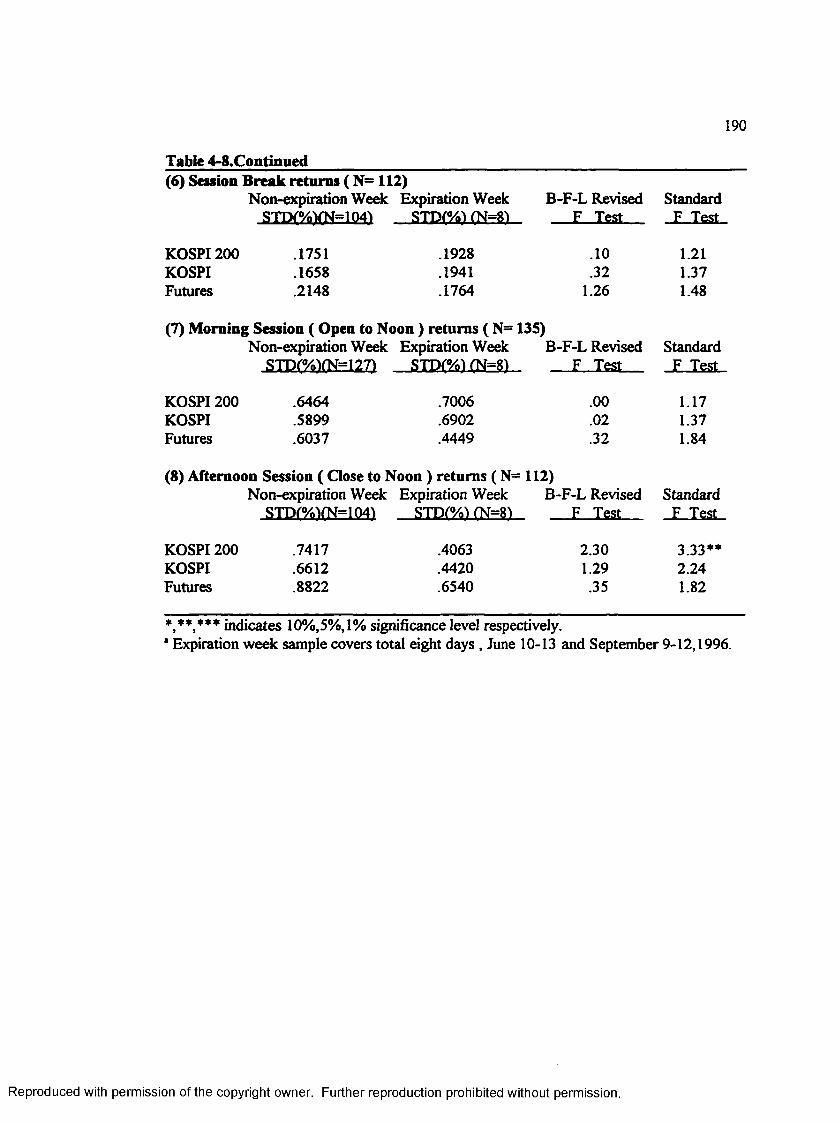
190
Table 4-g.Continued____________________________________________________(6) Session Break returns ( N= 112)
Non-expiration Week Expiration Week B-F-L Revised StandardSTD(%VN=1041 STD(%1 (N=81 F Test F Test
KOSPI 200 .1751 .1928 .10 1.21KOSPI .1658 .1941 .32 1.37Futures .2148 .1764 1.26 1.48
(7) Morning Session ( Open to Noon ) returns ( N= 135)Non-expiration Week Expiration Week B-F-L Revised Standard
STD(%)Ofel27) STPfift)flJ=8)... F . Tea F Test
KOSPI 200 .6464 .7006 .00 1.17KOSPI .5899 .6902 .02 1.37Futures .6037 .4449 .32 1.84
(8) Afternoon Session ( Close to Noon ) returns ( N= 112)Non-expiration Week Expiration Week B-F-L Revised Standard
STP(%XN=1Q4) . STP m ( N=8) - _ . E Teat JE_TesL
KOSPI 200 .7417 .4063 2.30 3.33**KOSPI .6612 .4420 1.29 2.24Futures .8822 .6540 .35 1.82
****** indicates 10%,5%,1% significance level respectively.1 Expiration week sample covers total eight days , June 10-13 and September 9-12,1996.
Reproduced with permission of the copyright owner. Further reproduction prohibited without permission.

191
Table 4-9. Trends of Daily Trading Volumes in Futures and KOSPI 200 1. June Contract Period ( 1996.5.3 - 1996.6.13)(1)KOSPI200 (1,000 shares)
Expiration Week* Non-Expiration Weeks Total
MeanMedian(2)Futures (Contracts)
10,50310.662
15,66613,548
15,05812,994
Eipiration Week Non-Expiration Weeks Total
MeanMedian
2,5802,872
3,2453,498
3,1673,413
2. September Contract Period ( 1996.6.14 - 1996.9.12) (1)KOSPI200 (1,000 shares)
Expiration Week Non-Expiration Weeks Total
Mean 7,551 7,377 7,386Median 7,766 7,317 7,317(2)Futures ( Contracts)
Expiration Week Non-Expiration Weeks Total
Mean 2,871 2,889 2,888Median 3,009 3,028 3,028
3. December Contract Period (1996.9.13 - 1996.10.16)(1)KOSPI200 (1,000 shares)
Before 1996.10.1b After 1996.10.1 Total
MeanMedian(2)Futures ( Contracts)
8,6178,862
Before 1996.10.1
19,70618,597
After 1996, 1Q.1
14,38312,251
Total
MeanMedian
3,9674,225
4,3844,721
4,1834,449
* Expiration week covers June 10-13 for June contract period and September 9-12 for September contract period.b The ceiling of foreign share ownership in the Korean stock market was raised by additional 2% from 18% to 20% on October 1, 1996. Therefore, stock trading volumes after this date may reflect temporary increase in buying force by foreign investors.
Reproduced with permission of the copyright owner. Further reproduction prohibited without permission.
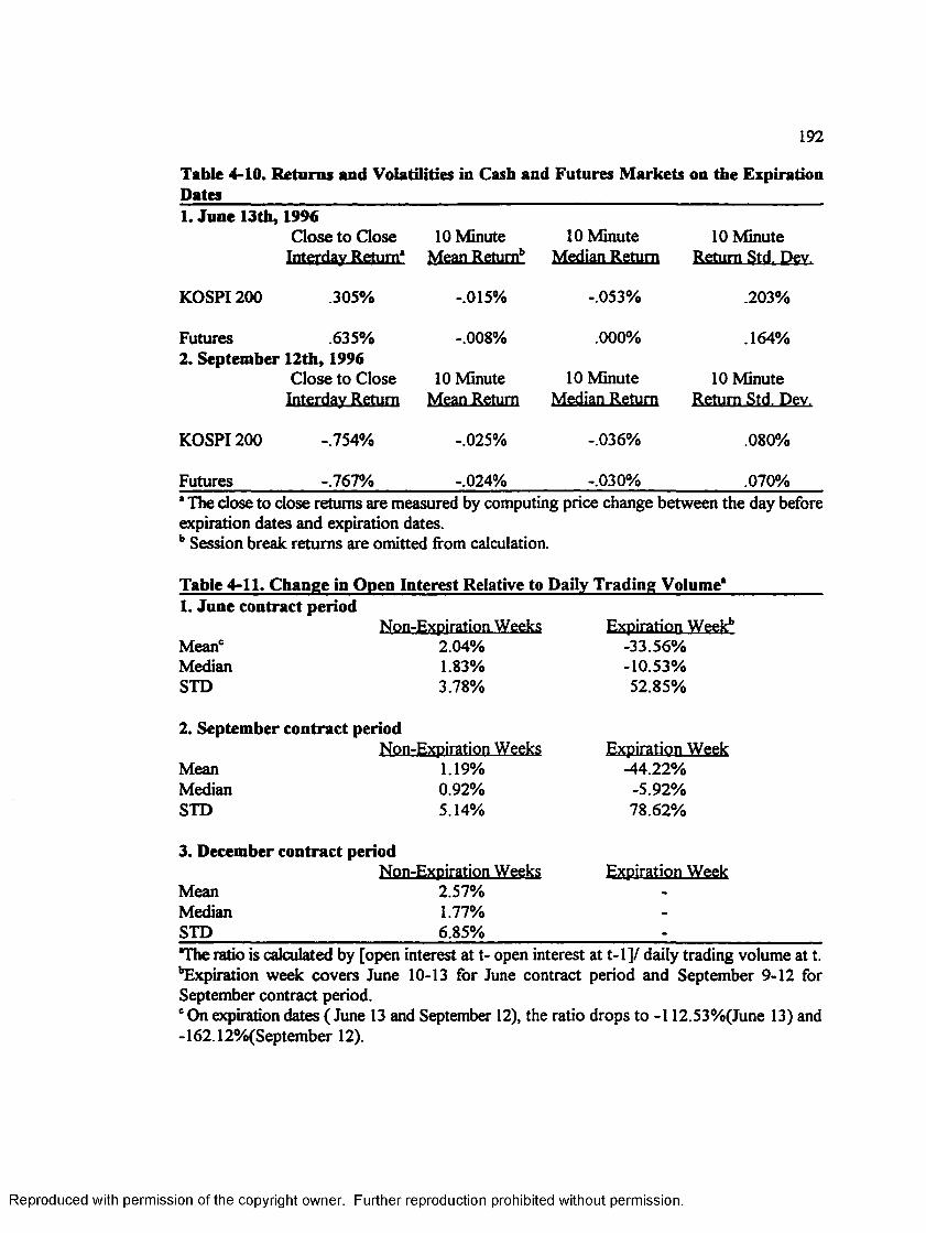
192
Table 4-10. Returns and Volatilities in Cash and Futures Markets on the Expiration Dates1. June 13th, 1996
Close to Close 10 Minute 10 Minute 10 MinuteInterdav Return* Mean Retumb Median Return Return Std. Dev.
KOSPI 200 .305% -.015% -.053% .203%
Futures .635% -.008% .000% .164%2. September 12th, 1996
Close to Close 10 Minute 10 Minute 10 MinuteInterday Return Mean Return Median Return Return Std. Dev.
KOSPI 200 -.754% -.025% -.036% .080%
Futures -.767% -.024% -.030% .070%* The close to close returns are measured by computing price change between the day before expiration dates and expiration dates. b Session break returns are omitted from calculation.
Table 4-11. Change in Open Interest Relative to Daily Trading Volume*1. June contract period
Non-Expiration Weeks 2.04%1.83%3.78%
Mean0MedianSTD
Expiration Week6 -33.56% -10.53% 52.85%
2. September contract periodNon-Expiration Weeks
Mean 1.19%Median 0.92%STD 5.14%
Expiration Week -44.22% -5.92% 78.62%
3. December contract periodNon-Expiration Weeks
Mean 2.57%Median 1.77%STD 6.85%
Expiration Week
The ratio is calculated by [open interest at t- open interest at t-1]/ daily trading volume at t. '’Expiration week covers June 10-13 for June contract period and September 9-12 for September contract period.0 On expiration dates ( June 13 and September 12), the ratio drops to -112.53%(June 13) and -162.12%(September 12).
Reproduced with permission of the copyright owner. Further reproduction prohibited without permission.
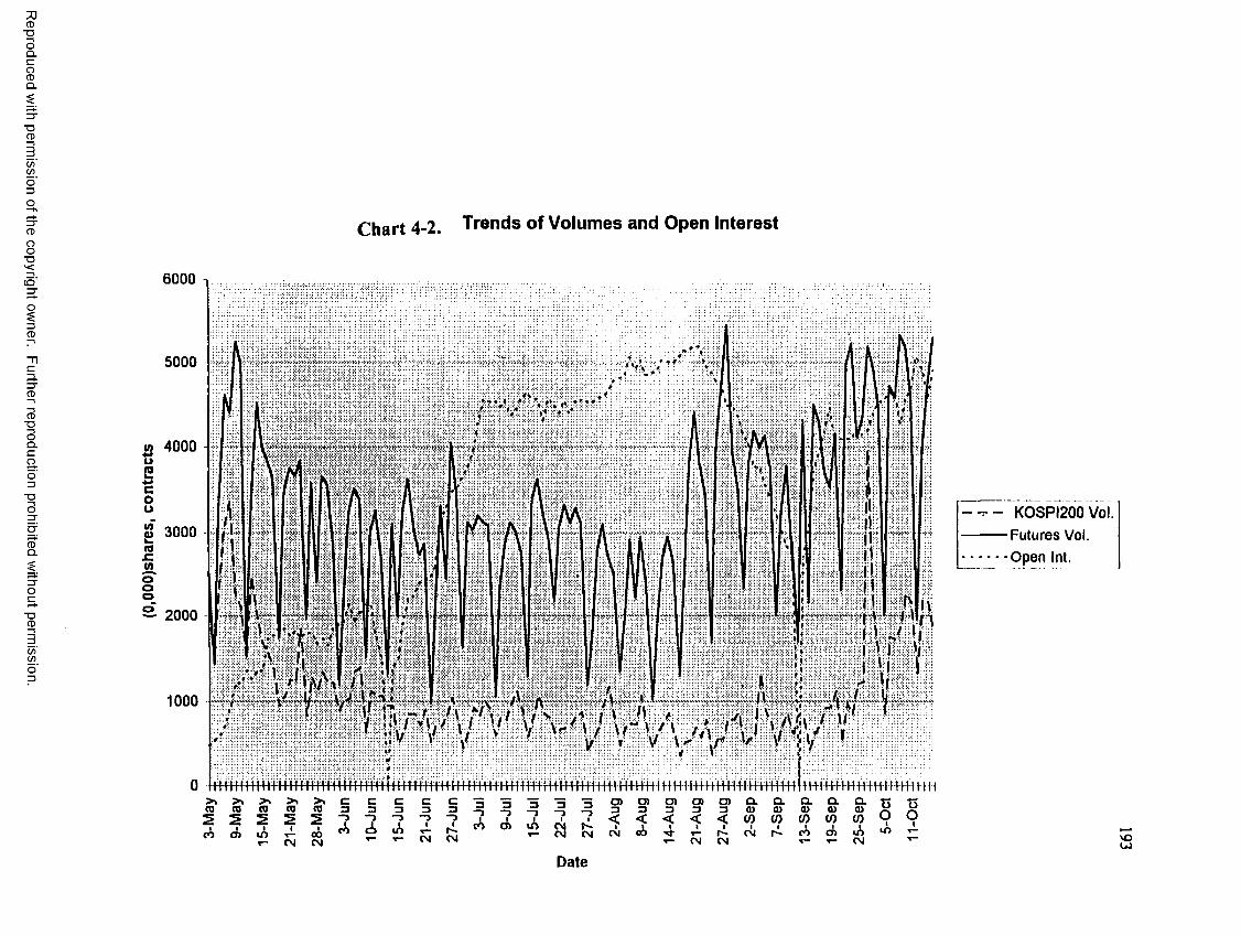
Reproduced
with perm
ission of the
copyright ow
ner. Further
reproduction prohibited
without
permission.
Chart 4-2. Trends of Volumes and Open Interest
6000
5000
40002OE**coo</»Sn£JOoooS- 2000
3000
1 0 0 0
t \
» » »
M J
/ ' * ' \ I ) | | t I . I \
• ' ' -> I\ \ « < , A n A . i ' \ } i ’i :;V Y >/ V '/ / V“V w VlV »
* r / \ / ':::'x: > • : : ; v;:Y:k.:.• : : : : : : : : • ::• • • ■:
‘; : : : : : : : : : : : r I : i i ; I ' ; : Y i • : : : : •; : : : I Y : ; Y : :
H-tH-mHttHltHMtrtttH I n il t H H W t H t H H HHUHH l-H HttH HUH t H HH H111 HUH ft t-HHl IH f H+H HttfHH H IIH I HHIttil>» >% >» >> >> c c c C C 3 3 CD O ) O ) O ) O ) Q . Ol a Q . a.CD <0 CD CD CD 3 3 3 3 3 s 3 3 3 3 3 0) CD Q> CD CDSco
Sd>
Sio
2i
2OO
“ J •3c i
tT“
“ 51 i
cOi
a>
31m
31CMCM
31N-CM CM
<OO
<t•M-
<iCO
1CM
(01
r-*COiCO
COia>
COim
eg CM p“ CN eg CM CM V *C“ CM
TSO 13O
KOSPI200 Vol. •Futures Vol. •Open Int.
oU)Date

Reproduced
with perm
ission of the
copyright ow
ner. Further
reproduction prohibited
without
permission.
Chart 4-3. Trend of the Ratio of Change in Open Interest to Daily Futures Volume
20 .000%
15.000%
10.000%
5.000%
o0 .000%
-5.000%
- 10 .000%
-15.000%
20.000% ■wmtitw iHHiutift HiuHt l iii i i i iumHii ii ii i ini itin t iHfittmiii iMim m n t i in iHiiiiiii fif> . > . > . > . c c c cz — □ ) □ ) a o i o .
i i i i J L . A r i J . ' f O O ' O c O Ot- cm co
T— T— (N i 1 - T - CM
m i m m m in n i i i mi Ha a a « tin> y y
OOCM
OO
\-— [open(t)-open(t-1)]/ volume(t) |
Date KOA

195
BIBLIOGRAPHY
Abhyankar, A.H., 1995, Return and Volatility Dynamics in the FT-SE 100 Stock Index and Stock Index Futures Markets, The Journal o f Futures Markets 15, 457-488.
Admati,AR. and Pfleiderer, P., 1988, A Theory of Intraday Trading Patterns : Volume and Price Variability, The Review o f Financial Studies 1, 3-40.
Bacha, O. and Vila,AF., 1994, Futures Markets, Regulation and Volatility : The Case of the Nikkei Stock Index Futures Markets, Pacific-Basin Finance Journal 2, 201-225.
Bailey,W., 1989, The Market for Japanese Stock Index Futures : Some Preliminary Evidence, Journal o f Futures Markets 9, 283-295.
Battacharya, AK. and Sundaram, S., 1986, The Effect of Futures Price Volatility on the Price Volatility of Treasury Bonds, Advances in Futures and Options Research 1, 193-213.
Bessembinder, H. and PJ.Seguin, 1992, Futures -Trading Activity and Stock Price Volatility, Journal o f Finance 47, 2015-2034.
Bessembinder, H. and PJ.Seguin, 1993, Price Volatility, Trading Volume, and Market Depth : Evidence from Futures Markets, Journal o f Financial and Quantitative Analysis 28, 21- 39.
Bessembinder,H., Chan, K. and PJ.Seguin, 1996, An Empirical Examination of Information, Differences of Opinion, and Trading Activity, Journal o f Financial Economics 40, 105-134.
Black, F., 1976, The Pricing of Commodity Contracts , Journal o f Financial Economics 3, 167-179.
Block, W.A. and Kleidon, A.W., 1992, Periodic Market Closure and Trading Volume : A Model of Intraday Bids and Asks, Journal o f Economic Dynamics and Control 16, 451-489.
Board, J. and C.Sutcliffe, 1995, The Relative Volatility of the Markets in Equities and Index Futures, Journal o f Business Finance and Accounting 22, 201-223.
Brennan, M. J., 1986, A Theory of Price Limits in Futures Markets, Journal o f Financial Economics 16, 213-233.
Brennan, M and Schwartz, E.,1990, Arbitrage in Stock Index Futures, Journal o f Business 63, S7-S31.
Brenner, M , Subrahmanyam, MG. and Uno, J . , 1989, The Behavior of Prices in the Nikkei Spot and Futures Market, Journal o f Financial Economics 23, 363-383.
Reproduced with permission of the copyright owner. Further reproduction prohibited without permission.
196
Brenner, M , Subrahmanyam, M.G. and Uno, J. ,1990, Arbitrage Opportunities in the Japanese Stock and Futures Markets, Financial Analysts Journal 46, 14-24.
Brown, MB. and Forsythe, A.B., 1974, Robust Tests for the Equality of Variances, Journal o f the American Statistical Association 69, 364-367.
Buhler,W.and Kempf, A., 1995, DAX Index Futures : Mispricing and Arbitrage in German Markets, Journal o f Futures M arket 15, 833-859.
Cakici N. and Chatteijee, S., 1991, Pricing Stock Index Futures with Stochastic Interest Rates, Journal o f Futures Markets 1991, 441-452.
Chan, K., 1992, A Further Analysis of the Lead-Lag Relationship between the Cash Market and Stock Index Futures Market, The Review o f Financial Studies 5, 123-152.
Chan, K., K.C.Chan and G.A_Karoiyi, 1991, Intraday Volatility in the Stock Index and Stock Index Futures Market, The Review o f Financial Studies 4, 657-684.
Chan, K. and Y.P.Chung, 1993, Intraday Relationships among Index Arbitrage, Spot and Futures Price Volatility, and Spot Market Volume : A Transaction Data Test, Journal o f Banking and Finance 17, 663-687.
Chan, K. and Y.P. Chung, 1995, Vector Autoregression or Simultaneous equations Model? The Intraday relationship Between Index Arbitrage and Market Volatility, Journal o f Banking and Finance 19, 173-179.
Chang, E.C., Jain, P.C. and Locke, P.R., 1995, Standard & Poor’s 500 Index Futures Volatility and Price Changes around the New York Stock Exchange Close, Journal o f Business 68, 61-84.
Chartrath, A., Ramchander, S. and Song, F., 1995, Does Options Trading Lead to Greater Cash Market Volatility ?, Journal o f Futures M arkets 15, 785-803
Chen, NJF., Cuny,C.J. and Haugen, R.A., 1995, Stock Volatility and the Levels of the Basis and Open Interest in Futures Contracts, Journal o f Finance 50, 281-300.
Cheung, Y.W. and Ng, L.K., 1990, The Dynamics of S&P 500 Index and S&P 500 Futures Intraday Price Volatilities, The Review o f Futures Market 9, 458-486.
Cheung, Y.W. and Ng, L.K., 1996, A Causality in Variance Test and its Application to Financial Market Prices, Journal o f Econometrics 72, 33-48.
Reproduced with permission of the copyright owner. Further reproduction prohibited without permission.

197
Chu, C.C. And Bubnys, E.L., 1990, A Likelihood Ratio Test of Price Volatilities : Comparing Stock Index Spot and Futures, Financial Review 25, 81-94.
Chung, YP, 1991, A Transactions Data Test of Stock Index Futures Market Efficiency and Index Arbitrage Profitability, Journal o f Finance 46, 1791-1809.
Comell,B. and Reinganum, M.R., 1981, Forward and Futures Prices : Evidence From the Foreign Exchange Markets, Journal o f Finance 36, 1035-1045
Cornell, B and French, K.R., 1983, The Pricing of Stock Index Futures, Journal o f Futures M arkets3, 1-14.
ComeUp., 1985, Taxes and the Pricing of Stock Index Futures : Empirical Results, Journal o f Futures M arkets 5, 89-101.
Cox, J.C., Ingersoll Jr., J.E. and Ross,S. A., 1981, The Relation between Forward prices and Futures Prices, Journal o f Financial Economics 9, 321-346.
Crain, S.J. and Lee, J.H., 1996, Volatility in Wheat Spot and Futures Markets, 1950-1993: Government Farm Programs, Seasonality, and Causality, Journal o f Finance 51,325-343.
Daigler, R.T., 1997, Intraday Futures Volatility and Theories of Market Behavior, Journal o f Futures M arkets 17, 45-74.
Davidian, M and Carroll, R.J., 1987, Variance Function Estimation, Journal o f American Statistical Association 82, 1079-1091.
Dickey, D.A. and Fuller, W.A., 1979, Distribution of the Estimates for Autoregressive Time Series with a Unit R oot, Journal o f the American Statistical Association 24, 427-431.
Dubofsky, D.A., 1992, Options and Financial Futures: Valuation and Uses, ( McGraw-Hill, New York).
Dusak, K., 1973, Futures Trading and Investor Return: An Investigation of Commodity Market Risk Premiums, Journal o f Political Economy 81, 1387-1406.
Dwyer, Jr.G.P., Locke, P. and Yu, W., 1996, Index Arbitrage and Nonlinear Dynamics Between the S&P 500 Futures and Cash, Review o f Financial Studies 9, 301-332.
Edwards, F.R.,1988, Does Futures Trading Increase Stock Market Volatility ?, Financial Analysts Journal 44, 63-69
Reproduced with permission of the copyright owner. Further reproduction prohibited without permission.

198
Ekman, P.D., 1992, Intraday Patterns in the S&P 500 Index Futures Market, Journal o f Futures M arkets 12, 365-381.
Elton,E.J., Gruber, M.J. and Rentzler, J.C., 1984, Intraday Tests of the Efficiency of the Treasury Bill Futures Market, Review o f Economics and Statistics 66, 129-137.
Engle, R.F. and Granger, C.W.J., 1987, Co-Integration and Error Correction : Representation, Estimation, and Testing, Econometrica 55,251-276.
Engle, R.F. and Granger, C.W.J., 1991, Long Run Economic Relationships, Readings in Cointegration, (New York, Oxford University Press).
Engle, R.F. and B.S.Yoo, 1987, Forecasting in Co-Integrated Systems , Journal o f Econometrics 35, 143-159.
Engle, R.F. and Ng,V.K., 1993, Measuring and Testing the Impact of News on Volatility, Journal o f Finance 48, 1749-1778.
Figlewski, S., 1984a, Hedging Performance and Basis Risk in Stock Index Futures, Journal o f Finance 39, 657-669.
Figlewski, S., 1984b, Explaining the Early Discounts on Stock Index Futures : The Case for Disequilibrium, Financial Analysts Journal 40, 43-47.
Finnerty, J.E. and Park, H.Y., 1987, Stock Index Futures : Does the Tail Wag the Dog ?, Financial Analysts Journal 43, 57-61.
Finnerty, J.E. and Park,H.Y., 1988, Intraday Returns and Volatility Patterns in the Stock Market: Futures Versus Spot, Advances in Futures and Options Research 3 : Fabozzi F. J. ed, 301-317.
Fleming, J., 1994, On the Comparison of Index Volatility in the Stocks and Futures Markets: A Commentary on Intraday and Overnight Volatility of Stock Index and Stock Index Futures Returns, Review o f Futures Markets 13, 31-38.
Fleming, J., Ostdiek,B. and Whaley, R.E., 1996, Trading Costs and the Relative Rates of Price Discovery in Stock, Futures, and Option Markets, Journal o f Futures M arkets 16, 353- 387.
Flesaker, B., 1991, The Relationship between Forward and Futures Contracts : A Comment, Journal o f Futures Markets 11, 113-115.
Reproduced with permission of the copyright owner. Further reproduction prohibited without permission.

V
199
French, K.R., 1983, A Comparison of Futures and Forward Prices, Journal o f Financial Economics 12, 311-342.
French, K.R. and Roll, R., 1986, Stock Returns Variances : The Arrival of Information and the Reaction of Traders, Journal o f Financial Economics 17, 5-26.
FrenchJC.R, Schwert, G. and Stambaugh, R.F., 1987, Expected stock Returns and Volatility, Journal o f Financial Economics 19, 3-29.
Garbade, K.D. and Silber, W.D., 1983, Price Movements and Price Discovery in Futures and Cash Markets, Review o f Economics and Statistics 65, 289-297.
Garman, M.B. and Klass,M.J., 1980, On the Estimation of Security Price Volatilities from Historical Data, Journal o f Business 53, 67- 78.
Geweke, J., Meese, R., and Dent, W., 1983, Comparing Alternative Tests of Causality in Temporal Systems : Analytic Results and Experimental Evidence, Journal o f Econometrics 21, 161-194.
Hamao,Y., Mauslis, R.W., and Ng. V., 1990, Correlations in Price Changes and Volatility across International Stock Markets, The Review o f Fiancial Studies 3, 281-307.
Harris, L., 1986, A Transaction Data Study of Weekly and Intraday Patterns in Stock Returns, Journal o f Financial Economics 16, 99-117.
Harris, L., Sofianos,G. and Shapiro,J.E., 1994, Program Trading and Intraday Volatility, The Review o f FinancialStudies 7, 653-685.
Herbst, AF., McCormack, I.P. and West,E.N., 1987, Investigation of a Lead-Lag Relationship between Spot Stock Indices and Their Futures Contracts, Journal o f Futures M arkets 7, 373-381.
Hsia,C.C., Fuller,B.R. and Kao,G.W., 1994, A Modified Method for Inferring the Effective Bid-Ask Spread from Security Returns, Journal o f Business Finance and Accounting 21, 243-253.
G.L. Gannon, 1994, Simultaneous Volatility Effects in Index Futures, Review o f Futures M arkets 13, 1027-1066.
Gastineau, G.L. and Madansky.A,1984, Standard & Poor’s 500 Composite Index Futures Evaluation Tables, in : Fabozzi, FJ. and Kipnis,G.M., eds.: Stock Index Futures, ( Dow Jones-Irwin, Homewood).
Reproduced with permission of the copyright owner. Further reproduction prohibited without permission.
200
Grossman, S. J., 1989, The Informational Role o f Prices, (Cambridge, The MIT Press).
Hamilton, J.D., 1994, Time Series Analysis, ( New Jersey, Princeton Univeristy Press).
HansonTiN. and Kopprasch, R.W., 1984, Pricing of Stock Index Futures, in : Fabozzi, F.J. and Kipnis,G.M., eds.: Stock Index Futures, (Dow Jones-Irwin .Homewood).
Ehara, Y., Kato, K. and Tokunaga,T., 1996, Intraday Return Dynamics between the Cash and the Futures Markets in Japan, Journal o f Futures Markets 16, 147-162.
Jarrow,R.A_ and Oldfield, G.S., 1981, Forward Contracts and Futures Contracts, Journal o f Financial Economics 9, 373-382.
JokivuoUe, E., 1995, Measuring True Stock Index Value in the Presence of Infrequent Trading, Journal o f Financial and Quantitative Analysis 30, 455-464.
Kim, I.W. and Yoon, T.S., 1992, An Investor’s Guide to the Korean Capital Market, (Quorum Books, Westport, Connecticut).
Kipnis,G.M. and Tsang,S., 1984, Classical Theory, Dividend Dynamics, and Stock Index Futures Pricing, in : Fabozzi, F.J. and Kipnis,G.M., eds.: Stock Index Futures, (Dow Jones- Irwin , Homewood).
Kipnis,G.M and Tsang,S., 1984, Arbitrage, in : Fabozzi, F.J. and Kipnis,G.M., eds.: Stock Index Futures, ( Dow Jones-Irwin .Homewood).
Kyle, A.S., 1985, Continous Auctions and Insider Trading, Econometrica 53, 1315-1335.
Kawaller.I.G., 1987, A Note : Debunking the Myth of the Risk-Free Return, Journal o f Futures Markets 7, 327-331.
Kawaller.I.G., 1991, Determining the Relevant Fair Value(s) of S&P 500 Futures: A Case Study Approach, Journal o f Futures M arkets 11, 453-460.
Kawaller,I.G., Koch, P.D. and Koch,T.W., 1987, The Temporal Price Relationship between S&P 500 Futures and the S&P 500 Index, Journal o f Finance 42, 1309-1329.
Kawaller,I.G., Koch, P.D. and Koch,T.W., 1990, Intraday Relationships between Volatility in S&P 500 Futures Prices and Volatility in the S&P 500 Index, Journal o f Banking and Finance 14, 373-397.
Koch, P.D., 1993, Re-examining Intraday Simultaneity in Stock Index Futures Markets, Journal o f Banking and Finance 17, 1191-1205.
Reproduced with permission of the copyright owner. Further reproduction prohibited without permission.

201
Korean Economic Daily (KED)
Lamoureux, C.G., and Lastrapes, W.D., 1990, Heteroskedasticity in Stock Return Data : Volume versus GARCH Effects, Journal o f Finance 45, 221- 229.
J.H.Lee and S.C.Linn, 1994, Intraday and Overnight Volatility of Stock Index and Stock Index Futures Returns, Review o f Futures M arkets 13, 1-30.
Levene, H., 1960, Robust Tests for Equality of Variances, Contributions in Probability and Statistics, Olkin I. (edited), (Palo Alto, California, Stanford University Press)
Levy, A., 1989, A Note on the Relationship between Forward and Futures contracts, Journal ofFutures M arkets 9, 171-173.
Lo, A.C. and A.C. MacKinlay, 1988, Stock Market Prices Do Not Follow Random Walks : Evidence From a Simple Specification Test, The Review o f Financial Studies 1, 41-66.
Lim, K.G., 1992, Arbitrage and Price Behavior of the Nikkei Stock Index Futures, Journal o f Futures M arkets 1992, 151-161.
A.C.MacKinlay and K.Ramaswamy, 1988, Index-Futures Arbitrage and the Behavior of Stock Index Futures Prices, The Review o f Financial Studies 1, 137-158.
MacKinnon, J., 1991, Critical values for Cointegration Tests , Long-Run Economic Relationships, Readings in Cointegration, R.F.Engle and C.W.J. Granger (edited), (New Y ork, Oxford University Press).
Maddala, G.S.,1992, Introduction to Econometrics, 2nd Edition, ( New York, MacMillan).
Martikainen,T., Perttunen, J. and Puttonen, V., 1995, On the Dynamics of Stock Index Futures and Individual Stock Returns, Journal o f Business Finance and Accounting 22, 87- 100.
Merrick, J.J.Jr.,1989, Early Unwinding and Rollovers of Stock Index Futures Arbitrage Programs : Analysis and Implications for Predicting Expiration Day Effects, Journal o f Futures M arket 9, 101-111.
Miller, M.H., Muthuwamy, J. and Whaley, R.E., 1994, Mean Reversion of Standard & Poor’s 500 Index Basis Changes: Arbitrage-induced or Statistical Illusion ?, Journal o f Finance 49, 479-513.
Reproduced with permission of the copyright owner. Further reproduction prohibited without permission.

202
Modest, DM. and Sundaresan, 1983, The Relationship between Spot and Futures Prices in Stock Index Futures Markets : Some Preliminary Evidence, Journal o f Futures M arkets 3, 15-41.
Ng, N., 1987, Detecting Spot Prices Forecasts in Futures Prices in Futures Prices Using Causality Tests, Review o f Futures Markets 6, 250-267.
Park,K.K.H. and Van Agtmael, AW., 1993, The World’s Emerging Stock Markets, (Probus Publishing Company, Chicago).
Parianson,M., 1980, The Extreme Value Method for Estimating the Variance of the Rate of Return, Journal o f Business 53, 61-66.
Pirrong, C., 1996, Market Liquidityand Depth on Computerized and Open Outcry Trading Systems : A Comaprison of DBT and L1FFE Bund Contracts, Journal o f Futures M arkets 16, 519-543.
Quan, J., 1992, Two-Step Testing Procedure for Price Discovery Role of Futures Prices, Journal o f Futures M arkets 12, 139-149.
Rhee, S.G., 1992, Securities Markets and Systematic Risks in Dynamic Asian Economies, (OECD, Paris).
Roll, R, 1984, A Simple Implicit Measure of the Effective Bid-Ask Spread in an Efficient Market, Journal o f Finance 39, 1127-1139.
Ross, S.A., 1989, Information and Volatility : The No-Arbitrage Martingale Approach to Timing and Resolution Irrelevancy, Journal o f Finance 44, 1-17.
Sims, C., 1972, Money, Income and Causality, American Economic Review 62, 540-552.
Sims, C., 1980, Macroeconomics and Reality, Econometrica 48, 1-48.
Schwarz,T.V., 1991, The Relationship between Stock Indices and Stock Index Futures from 3:00 to 3:15 : A Clarification, Journal o f Futures M arkets 11, 647-649.
Schwert, G.W., 1989, Why does stock market volatility change over time ?, Journal o f Finance 44, 1115-1153.
Schwert, G.W., 1990, Stock Volatility and the Crash o f‘87, The Review o f Financial Studies 3, 77-102.
Reproduced with permission of the copyright owner. Further reproduction prohibited without permission.

203
Shyy, G., Vijayraghavan, V. and Scott-Quinn, B., A Further Investigation of the Lead-Lag Relationship between the Cash Market and Stock Index Futures Market with the Use of Bid/Ask Quotes: The case of France, Journal o f Futures M arkets 16, 405-420.
Smirlock, M. and L. Starks, 1986, Day of the Week and Intraday Effects in Stock Returns, Journal o f Financial Economics 17, 197-210.
Sofianos,G., 1993, Index Arbitrage Profitability, Journal o f Derivatives 1,7-20.
Stoll, HR. and Whaley, R.E., 1987, Program Trading and Expiration Day Effects, Financial Analysts Journal A3, 16-28.
Stoll, HR. and Whaley, R.E., 1990a, The Dynamics of Stock Index and Stock Index Futures Returns, Journal o f Financial and Quantitative Analysis 25, 441-468.
Stoll,HR. and Whaley, R.E., 1990b, Stock Market Structure and Volatility, The Review o f Financial Studies 3, 37-71.
Subrahmanyam, A., 1991, A Theory of Trading in Stock Index Futures, The Review o f Financial Studies A, 17-51.
Tauchen, G.E. and Pitts, M , 1983, The Price Variability-Volume Relationship on Speculative Markets, Econometrica 51, 485-505.
Wiggins, J.B., 1992, Estimating the Volatility of S&P 500 Futures Prices Using the Extreme- Value Method, Journal o f Futures Markets 12, 265-273.
Wood, R.A., McInish,T.H. and Ord, J.K., 1985, An Investigation of Transaction Data for NYSE stocks, Journal o f Finance 40, 723-741.
Yadav, P.K. and Pope, P.F., 1990, Stock Index Futures Arbitrage : International Evidence, Journal o f Futures M arkets 10, 573-603.
Reproduced with permission of the copyright owner. Further reproduction prohibited without permission.

204
APPENDIX
This appendix contains a list o f daily trading volumes o f the KOSPI 200 and the nearby futures contract and daily open interest of the nearby futures contract from May 3rd, 1996 - October 16th, 1996__________________________________________________________
Date KOSPI200 Futures OpenVolume (10,000shrs) Volume_____Interest
3-May 20,451 2,527 4794-May 15,374 1,428 5306-May 23,734 3,385 5927-May 30,901 4,614 7268-May 33,578 4,401 9589-May 22,640 5,250 1,22210-May 21,228 5,015 1,20811-May 15,065 1,667 1,34913-May 24,706 3,435 1,26514-May 20,129 4,521 1,35915-May 16,770 4,010 1,34916-May 15,462 3,835 1,72517-May 13,720 3,627 1,76818-May 9,455 1,731 1,85520-May 10,598 3,489 1,83621-May 12,510 3,751 1,75122-May 12,374 3,654 1,81623-May 18,369 3,842 1,73825-May 8,282 1,961 1,80027-May 12,759 3,575 1,79028-May 11,216 2,407 1,66629-May 13,230 3,647 1,72230-May 12,282 3,566 1,64731-May 12,154 2,932 1,8381-Jun 8,952 1,200 1,8923-Jun 10,110 2,232 1,9304-Jun 10,293 3,254 2,1355-Jun 13,375 3,506 1,9497-Jun 13,934 3,392 2,0428-Jun 6,323 1,509 2,13910-Jun 11,189 3,017 2,11911-Jun 10,731 3,259 1,73512-Jun 10,593 2,726 1,48213-Jun** 9,500 1,317 014-Jun 9,453 3,109 1,40315-Jun 5,022 1,989 1,50017-Jun 6,343 3,265 1,91618-Jun 8,520 3,622 2,218
Reproduced with permission of the copyright owner. Further reproduction prohibited without permission.

205
Appendix Continued19-Jun 8,481 3,052 2,23620-Jun 7,185 2,731 2,39021-Jun 9,039 2,859 2,44422-Jun 5,215 975 2,44824-Jun 7,143 2,125 2,58125-Jun 7,083 3,320 3,11726-Jun 8,299 2,449 3,28127-Jun 10,374 4,045 3,46928-Jun 7,929 3,444 3,50729-Jun 4,440 1,616 3,6201-Jul 6,537 3,128 3,7602-Jul 9,145 3,032 3,9233-Jul 8,236 3,196 4,2674-JuI 9,951 3,123 4,5515-Jul 9,258 3,086 4,5316-Jul 5,965 1,057 4,5518-Jul 7,964 2,368 4,4759-Jul 7,835 2,873 4,54610-Jul 9,679 3,122 4,37611-Jul 11,107 3,024 4,44412-Jul 9,019 2,762 4,55213-Jul 5,816 1,297 4,63715-Jul 7,853 3,394 4,57916-Jul 10,671 3,616 4,56818-Jul 8,666 3,241 4,31719-Jul 8,025 2,933 4,56920-Jul 6,278 2,177 4,48722-Jul 6,692 3,084 4,40423-Jul 6,814 3,327 4,54424-Jul 7,335 3,122 4,39025-Jul 8,241 3,289 4,54326-Jul 8,743 3,122 4,55227-Jul 4,418 1,201 4,55229-Jul 5,399 1,789 4,51330-JuI 6,768 2,808 4,57431-Jul 9,680 3,106 4,6051-Aug 11,748 2,710 4,6512-Aug 8,149 2,517 4,7743-Aug 4,874 1,353 4,8145-Aug 6,838 1,998 4,8306-Aug 7,338 2,907 5,0597-Aug 7,231 2,219 4,9228-Aug 10,578 2,945 5,0209-Aug 6,825 2,387 4,84810-Aug 4,482 1,026 4,87312-Aug 6,377 1,915 4,889
Reproduced with permission of the copyright owner. Further reproduction prohibited without permission.

206
Appendix Continued13-Aug 7,298 2,685 5,01814-Aug 8,526 2,955 5,01016-Aug 6,166 2,643 4,99517-Aug 3,605 1,300 5,07219-Aug 5,083 2,456 5,13820-Aug 5,413 3,814 5,15021-Aug 6,782 4,408 5,19922-Aug 5,799 3,797 5,18323-Aug 7,745 3,418 4,95424-Aug 3,754 1,683 4,87726-Aug 5,506 4,048 4,78427-Aug 5,480 4,758 4,74728-Aug 7,653 5,454 4,49329-Aug 7,856 3,941 4,48430-Aug 8,583 3,506 4,36831-Aug 4,849 2,336 4,1622-Sep 5,549 3,815 4,0293-Sep 6,165 4,191 3,7624-Sep 13,228 4,000 3,7745-Sq> 8,758 4,134 3,5556-Sep 7,506 3,774 3,4157-Sep 4,786 2,003 3,2469-Sep 7,130 3,237 3,06810-Sep 8,452 3,771 2,82911-Sep 6,225 2,780 2,74812-Sep** 8,397 1,695 013-Sep 7,950 4,311 2,69814-Sep 4,340 2,168 3,01716-Sep 6,286 4,495 3,70217-Sep 7,188 4,299 3,93918-Sep 9,177 3,700 4,17519-Sep 9,295 3,528 4,45220-Sep 11,153 4,150 4,05121-Sep 5,546 2,313 4,09223-Sep 9,653 4,986 4,10124-Sep 8,548 5,222 4,09725-Sep 12,019 4,116 4,21930-Sep 12 251 4,316 4,1521-Oct 39,659 5,190 4,1992-Oct 20,491 4,935 4,3904-Oct 14,680 4,449 4,5215-Oct 8,701 2,005 4,5537-Oct 17,470 4,721 4,6268-Oct 17,142 4,583 4,6509-Oct 18,597 5,326 4,27010-Oct 22,578 5,181 4,555
Reproduced with permission of the copyright owner. Further reproduction prohibited without permission.
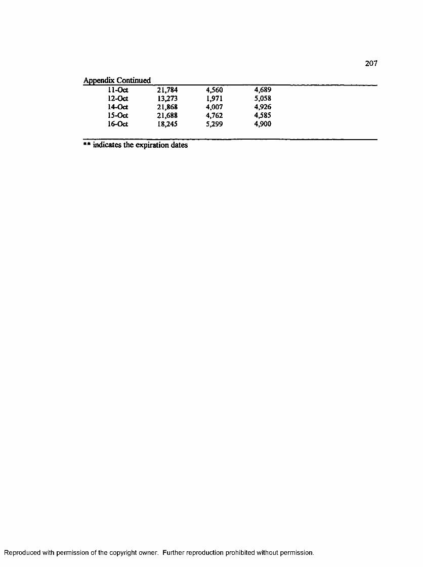
207
Appendix Continued11-Oct 21,784 4,560 4,68912-Oct 13,273 1,971 5,05814-Oct 21,868 4,007 4,92615-Oct 21,688 4,762 4,58516-Oct 18,245 5,299 4,900
** indicates the expiration dates
Reproduced with permission of the copyright owner. Further reproduction prohibited without permission.

VITA
Name in Full
Birth of Date
Professional Experience
Jun. 1992 to Jul. 1994
Oct. 1989 to May 1992
Aug. 1988 to Feb. 1989
Education
Aug. 1996
Dec. 1987
Feb. 1986
Jaehoon Min
July 29,1963
ManagerInternational Finance Department Daihan Investment & Finance Corp. Seoul, Korea
Investment Analyst Investment Research Department Korea Long Term Credit Bank Management Co.Seoul, Korea
Second Lieutenant Korean Army Youngchon, Korea
Master of Arts in Economics Old Dominion University Norfolk, Virginia
Master of Business Administration Major in FinanceUniversity of Wisconsin at Madison
Bachelor of Business Administration Major in Finance and Minor in Accounting Yonsei University Seoul, Korea
Reproduced with permission of the copyright owner. Further reproduction prohibited without permission.