The producer surplus

associated with gasoline fuel use in the United States1

Yongling Sun, Mark A. Delucchi, C.-Y. Cynthia Lin, Joan M. Ogden

Abstract

Estimating the producer surplus – the revenue above the average long-run cost – is an important part of social cost-benefit analyses of changes in petroleum use. This paper estimates the producer surplus associated with changes in gasoline fuel use in the United States, and then applies the estimates of producer surplus to two kinds of social cost-benefit analyses related to petroleum use: (1) estimating the wealth transfer from consumers to producers as a result of policies that affect oil use and oil imports to the US, and (2) comparing the actual average cost of gasoline with the average cost of environmentally superior alternatives to gasoline, such as hydrogen. Our results show that a 50% reduction in gasoline use in the US in 2004 would have saved the US $72 billion in producer surplus payments to foreign oil producers. Applying our estimates to the comparison of the social lifetime cost of hydrogen vehicles versus gasoline vehicles, we find that inconsistently counting producer surplus from a US national perspective while counting climate change damages from a global perspective can overstate the present value lifetime costs of gasoline vehicles by $2,200 to $9,800 per vehicle.

JEL codes: Q41, Q43 Keywords: oil, marginal costs, producer surplus, gasoline, wealth transfer, drilling costs, exploratory wells, development wells

1 We received financial support from the Sustainable Transportation Energy Pathways Program at the University of California at Davis Institute of Transportation Studies. Lin is a member of the Giannini Foundation for Agricultural Economics. All errors are our own.

1. Overview

Estimating the producer surplus – the revenue above the long-run average cost – is an important part of social cost-benefit analyses of changes in petroleum use. This paper estimates the producer surplus associated with changes in gasoline fuel use in the United States, and then applies the estimates of producer surplus to two kinds of social cost-benefit analyses related to petroleum use: (1) estimating the wealth transfer from consumers to producers as a result of policies that affect oil use and oil importing in the US, and (2) comparing the actual average cost of gasoline (where the average cost is the observed price minus the estimated fraction of price that is producer surplus) with the average cost of environmentally superior alternatives to gasoline, such as hydrogen. The first use of estimates of producer surplus in social cost-benefit analyses is to estimate wealth transfers as a result of policies affecting US oil use. Estimates of the producer surplus for gasoline can be used to better understand wealth transfers from oil consumers to oil producers, as part of an analysis of the total costs and benefits to the US of policies related to oil use and oil imports. The total producer surplus change is a measure of the wealth transfer from consumers to producers. We designate the producer surplus change as △PSt, where t stands for “transfer”. To estimate the transfer of wealth associated with oil use, we estimate the change in total producer surplus associated with different levels of reduction of oil supply. This change in total producer surplus has two parts: one due to the change in consumption, and the other due to the change in price. We estimate both of these formally. The second use of estimates of producer surplus in social cost-benefit analyses is to estimate the average cost of gasoline in cost-benefit analyses of transportation fuel policies. Owing in part to the environmental, economic and security concerns related to oil consumption and to concerns about the economic impact of high oil prices, there is considerable interest in understanding the social costs and benefits of policies that reduce gasoline use, especially policies that promote non-petroleum alternative transportation fuels. Estimates of the producer surplus fraction for gasoline can be used to estimate the average cost of gasoline in social cost-benefit comparisons of various transportation fuels, as well as in social cost-benefit analyses of other policies that reduces petroleum consumption, such as fuel economy improvements, carbon taxes, or the substitution of alternative fuels. We designate the producer surplus fraction of revenues as PSfac , where ac stands for “average cost”. Since cost-benefit analyses are concerned with real resource costs, the relevant measure of resource cost is the average cost, not price. However, while we can observe price, we cannot observe average cost directly, and if we have reason to believe that there is a large difference between observed price and average cost – for example, because oil-rich countries appear to accumulate great wealth, suggesting that their (price-times-quantity) revenue far exceeds their (average) cost – then it is important to estimate average cost explicitly rather than use price as a proxy for average cost. Consider the case of comparing the costs and benefits of transportation fuels. Under the

assumption that all transportation fuel options (including petroleum) offer the same non-cost vehicle amenities (performance, cargo capacity, etc.), and therefore have the same social benefits, these alternatives can be compared strictly on the basis of social cost. The social lifetime cost includes the cost of vehicles, the cost of fuel, and external costs such as air pollution damages, climate change impacts, noise, and oil security. Fuel (or resource) cost estimates can be made for non-petroleum fuels using engineering-economic models, but this is problematic for gasoline, because such detailed but generalizable engineering cost data are difficult to obtain. Instead, to estimate the average cost of gasoline, in a social cost-benefit comparison of gasoline with alternative non-petroleum fuels, we first estimate the producer surplus fraction of total price-times-quantity payments for different levels of reduction in the supply of gasoline, and then calculate gasoline average cost as the price minus the producer surplus fraction of price. For both of these cost-benefit analysis examples, we estimate the producer surplus for US petroleum refiners, the producer surplus for US oil producers, the producer surplus for the Organization of Petroleum Exporting Countries (OPEC), and the producer surplus for producers in the rest of the world (ROW). We do this for current and future oil supply. We pursue the following research questions. First, how can we use existing data to estimate gasoline cost curves? Second, what is the historical production cost for gasoline? Third, what is the producer surplus fraction for gasoline, historically and projected into the future? Fourth, what is the total producer surplus change, in the US, and abroad, associated with petroleum use reduction? And finally, what does this imply about the future competitiveness of alternative fuels compared to gasoline and about their wealth transfers? According to our results, both kinds of producer surplus estimates depend on the size of the reduction in oil use and the year and region for which oil cost curves are estimated. We estimate that if demand for gasoline in the US in 2004 had contracted by 10% (50%), then the change in producer surplus in the US refinery and US oil industry would have been $15.2 ($31.63) billion, or $4.84 ($1.86) per gallon of gasoline, and the producer surplus fraction of revenues would have been 31.89% (49.03%). The change in producer surplus for gasoline made from imported oil would have been greater – $5.48/gallon for a 10% contraction and $2.28/gal for a 50% contraction – because foreign producers have much lower average production cost. In fact, a 50% reduction in gasoline use in the US in 2004 would have saved the US $72 billion in producer surplus payments to foreign oil producers. Applying our estimates to the comparison of the social lifetime cost of hydrogen vehicles versus gasoline vehicles, we find that inconsistently counting producer surplus from a US national perspective while counting climate change damages from a global perspective can overstate the present value lifetime costs of gasoline vehicles by $2,200 to $9,800 per vehicle. We organize the paper as follows: Section 2 presents a detailed discussion of the producer surplus concept. Section 3 describes the general method of analysis, followed by a literature review in Section 4. Section 5 presents the detailed analysis, including data and methods used for constructing oil and gasoline cost curves. Section 6 analyzes the results, and Section 7

illustrates the use of estimates of producer surplus in an analysis of the changes in transfer of wealth from the US to foreign oil producers as a result of US oil conservation policies and in an analysis of the social cost of gasoline versus hydrogen. Section 8 concludes the paper.

2. Discussion of producer surplus

The total revenue a producer receives from selling a good in the market is the market price of the good times the quantity of the good sold. The total revenue comprises two parts: producer surplus and total cost. Producer surplus is the area above the producer’s marginal cost curve and below the price, and which measures the revenue, above and beyond cost, that a producer receives for selling a good in the market. The shaded area in Figure 1 indicates the producer surplus in an imperfectly competitive market for some firm with marginal cost MC0 below market price P0. We use an imperfectly competitive market in our illustration here because this better characterizes the world oil market, but, as we discuss below, producer surplus exists in perfectly competitive markets as well. The second part of the total revenue is the cost to the producers of producing the good, or the area under the long-run marginal cost curve, and represents the resource cost of producing the good.

Figure 1. Producer Surplus in an imperfect market

Note that for any price, cost curve, and quantity, as in Figure 1, there is an average cost line that gives the same producer surplus and total cost. When we refer to average cost in this paper, we mean the average cost that gives the same producer surplus and total cost as does the actual cost curve. Note also that we speak interchangeably of subtracting producer surplus from price-times-quantity revenues and subtracting from price the fraction of price that is producer surplus, because the fraction of price that is the producer surplus is equal to the ratio of producer surplus over price-times-quantity revenues. Note also that because the world oil market is not perfectly competitive, the supply curve is not necessarily the same as the long-run marginal cost curve. The producer surplus is a wealth transfer from consumers to producers within the society, not an economic cost. When alternative fuels are compared using a social cost-benefit analysis, the

comparison should be based on their long-run marginal cost curve, or average cost, and producer surplus should be viewed as a social transfer instead of a cost and therefore should not “count” as a social cost. To clarify the importance of comparing alternatives on the basis of economic cost (and hence of subtracting producer surplus from revenues), we use the following example. Table 1 presents a case with two fuel types I and II produced by two different firms A and B, respectively. Suppose markets for both fuels are perfectly competitive in long-run equilibrium with no market failures or any externalities, and they provide the user identical benefits. The only difference is in the production cost, which is $20/MBTU for Firm A and $40/MBTU for Firm B. The difference is that firm A is endowed with large reserves of fuel I that can be recovered easily with little effort; specifically, the labor requirement by firm A is only half of that by firm B for the same production level. It is clear that society prefers fuel I because it has lower social resource cost for the same level of benefits. However, for our cost-benefit analysis to reflect this, we either must estimate the long-run marginal cost curve (or average cost) directly (from the “bottom up,” based on the amount and cost of individual inputs), or else subtract the producer surplus from the price-times-quantity revenues. Table 1. Two-fuel case

Firm A Firm B Fuel type I IISelling price $50/BTU $50/BTUValue to consumer $55/BTU $55/BTUMarginal cost of production $20/BTU $40/BTUProducer surplus $30/BTU $10/BTU In imperfectly competitive markets such as the oil market, the concentration of low-cost resources in a handful of countries and the oligopolistic nature of the market enable the producers to affect prices by controlling output. Oil suppliers produce less oil than they would under perfect competition and as a result the oil market price can exceed marginal cost. As a consequence producers can have a rate of return greater than the normal rate of return. In contrast, in a perfectly competitive market the competition in the industry would drive the market to a long-run equilibrium in which price would equal marginal cost. Thus each firm would earn the normal rate of return and zero economic profit. However, even in perfect competition owners of low-cost oil resources still would receive producer surplus as economic rent. The following is an example to illustrate these economic concepts.2 Suppose an oil producer owns a parcel of an oil field. The total revenue from selling oil from the field is $75M, in an 2 For a definition of some terms related to producer surplus, see Table A1 and Figure A1, both in Appendix A.

imperfect market, and the only input is capital (no labor). The producer could earn $30M if she invests the capital into the next best business; hence, the capital cost – which in this case is the total economic cost – is $30M. The producer surplus is the total revenue less the economic cost: $75M-$30M=$45M. Now, assume the revenue would be $65M if the market were perfect. Thus the economic rent associated with the land is $65M-$30M=$35M. The economic profit is $75M-$65M=$10M (the difference between the actual revenue and the revenue that would be were the market perfect). It is important to note that in a competitive market economic profit is zero in the long-run equilibrium but producer surplus generally is not zero. Producer surplus comprises economic profit and economic rent (see Figure A1 of Appendix A), and in a competitive market there is only normal profit, not economic profit, but generally there is economic rent. The amount of economic rent is determined by the relationship between average cost and the competitive market price; the lower the average cost relative to the competitive price, the greater the economic rent and the greater the producer surplus. The average cost will be relatively low if many producers are endowed with low-cost resources and hence have low economic cost, and if a handful of “marginal” producers have high long-run marginal costs and determine the relatively high competitive market price. This is precisely the situation in the oil industry, where there is a large difference between the low cost of producing oil from a giant field in Saudi Arabia and the high cost of producing low quality oil from deepwater wells. On top of this large economic rent, oil producers also enjoy economic profit, because the oil market is not competitive, and this adds to oil industry producer surplus. It also is useful to examine economic rent more closely, to understand why it is a transfer between consumers and producers, or between producers, and not a net economic cost to society. The abundant and cheap petroleum resources (oil rights) for those countries originally endowed with the low-cost oil are valuable and other entities would be willing to pay for them. In a competitive market with competitive bidding, the maximum amount that other entities would be willing to pay for these rights to low-cost oil is the difference between the market price and the average economic production cost (including normal profit). The firms buying these oil rights would count this maximum payment as a cost. However, this cost is just a transfer payment to the original owners of the low-cost oil, for whom the payment is economic rent above their actual economic cost. Thus, economic rent, even when accounted as a “cost” by firms paying for the oil rights, is just a transfer payment, and not a real economic (resource) cost the way drilling costs are. From a global perspective, producer surplus is a transfer from consumers to producers, and the location of the consumers and producers does not matter. However, if one conducts a social cost-benefit analysis for a particular country (e.g., the US), then one does not count the welfare of consumers or producers outside of that country. In this case, a producer surplus transfer from domestic consumers to foreign producers is in fact a real wealth loss for the country in question, because the welfare of foreign producers is not counted in a country-specific analysis and as a

result the loss to consumers is not balanced by a gain to producers. Estimating the producer surplus is therefore an important part of social cost-benefit analyses of changes in petroleum use. This paper estimates the producer surplus associated with changes in gasoline fuel use in the United States, and then applies the estimates of producer surplus in two kinds of social cost-benefit analyses related to petroleum use: (1) estimating the wealth transfer from consumers to producers as a result of policies that affect oil use and oil importing in the US, and (2) comparing the actual average cost of gasoline (where the average cost is the observed price minus the estimated fraction of price that is producer surplus) with the average cost of environmentally superior alternatives to gasoline, such as hydrogen.

3. General method of analysis

In order to estimate the producer surplus associated with transportation fuels, we must first estimate the cost curves for petroleum fuels. With the estimated cost curves, we can estimate the average cost as a fraction of price (the complement of PSfac). We estimate the average cost fraction, rather than the absolute average cost, because the average cost fraction presumably varies much less over time than does the absolute average cost. This analysis begins with a construction of the US oil cost curve based on the most recent data publicly available from American Petroleum Institute (API). We then derive the gasoline cost curve assuming that oil and gasoline costs have the same correlation as their prices, and use this to estimate the producer surplus for gasoline. Three energy projection scenarios from the Energy Information Administration (EIA) Annual Energy outlook (AEO) 2009 are also examined to project future oil and gasoline cost curves for the producer surplus calculations. In general, total oil supply costs comprise exploration and development costs, which are capital intensive, and production costs, which include operating and maintenance. According to the API data in 1989, the most recent year where disaggregated costs data are available, the estimated cost of drilling and equipping exploratory oil and gas wells was about 35% of total exploration cost, and the estimated cost of drilling and equipping development was about 60% of total development cost (API, 1989). The cost of drilling wells is determined mainly by the well depth, diameter, casing design, and location-specific characteristics. However, a large number of factors and events impact drilling performance, and it is complex and challenging to quantify well costs (Kaiser, 2007). Fortunately, the API’s Joint Association Survey (JAS) is an authoritative source for drilling costs. The JAS employs a statistical model to estimate drilling cost using survey data. Tabulated data of average costs for drilling wells in the US from the JAS on drilling costs for the period 1976 to 2004 show a general trend that drilling costs increase non-linearly with depth intervals (API, 2004; Augustine et al., 2006). We use the most recent JAS data, which are for the year 2004, to construct an oil cost function for the year 2004.3

3 Note, however, that other sources suggest that oil supply costs have increased appreciably since 2004.

From the JAS and EIA data (EIA, 2009b) we can estimate the average production per well, and knowing the number of exploratory or development wells we can estimate the oil production in barrels. Based on historical data from API, we apply econometric modeling to derive functions for the relationships between oil production levels and oil exploration costs or oil development costs. To construct the marginal production cost curve (for the oil production stage), we assume it has an exponential shape, and then calibrate the parameters in the exponential function calibrated to fit data in years 2003 and 2004. Other exploration or development-related average costs are assumed to be independent of oil production level. The sum of all these costs generates the oil marginal cost curve for 2004. For future oil marginal cost curves, we develop a regression model to find the trend in the average cost over time and then shift the 2004 curve based on the projected average cost. Our analysis adopts the EIA AEO 2009 (EIA, 2009a) updated reference, high economic growth, low economic growth, high price and low price cases for the future oil supply, oil and gasoline prices, and reserves projected through 2030 in the US. These projections are based on results from the EIA’s National Energy Modeling System (NEMS). To estimate the gasoline cost curve, we assume that the relationship between gasoline costs (which we do not know) and oil costs (which we estimate) is the same as the relationship between gasoline prices and oil prices (both of which we know). We also estimate the oil cost curves for OPEC and ROW with data from World Bank as compared with the US case.

4. Literature Review

In this section, we review studies that are relevant to our general method of analysis, including studies of oil production cost, factors that affect oil supply cost according to theory, oil supply projection, and the estimation of producer surplus generally. Biedermann (1961) estimates a cost function for crude oil production based on empirical data, considering three major factors that affect the cost of getting crude oil from the reservoir to the top of well: drilling costs, well operating costs and the cost of physical waste and depletion. The US average drilling cost per well and average depth per well in 1953 are fitted with a quadratic function. Linear cost-output relationships within certain limits are assumed for well operating costs for both short-run and long-run considerations. Depletion and waste costs are modeled as a function of production rate, exploitation rate, expected oil price, reservoir (or oil field) lifetime and interest rate. A hypothetical relationship is assumed between exploitation rate and production rate, which is only valid for a given production mechanism under certain geological conditions of a reservoir.

According to the IEA World Energy Outlook 2009 (IEA, 2009), the worldwide upstream oil and gas capital expenditures significantly increased between 2004 and 2008, from about $220 billion in 2004 to around $480 billion in 2008. The escalating expenditures on oil exploration and developments suggest that oil cost became much higher beyond 2004. However, since we are unable to obtain international data beyond 2004, we focus on the period 1976 to 2004.

Cleveland (1991) argues that two opposing forces -- technical change and resource depletion -- determine the long-run average cost of oil discovery and production. A U-shaped cost path hypothesis is empirically tested with the lower 48 US data from 1936 to 1988 on the quantity and dollar cost of oil added to reserves and oil extracted. Chakravorty et al. (1997) estimate the extraction cost for energy resources as a nonlinear function of cumulative extraction and analyze the effects of technological change in cost reductions for the backstop technology for resource extraction. Stock effects and technological progress are further examined by Lin and Wagner (2007), who extend the Hotelling model (Hotelling, 1931) of optimal resource extraction and find that in order for market prices to be constant and consistent with the empirical observation that the growth rates of market prices have remained zero over a long period of time, the ratio of technological progress to the stock effect must exactly offset the exogenous growth in demand. Aguilera (2014) reviews several methods for assessing current and long-term production costs of petroleum. For the cumulative availability curve showing total costs and total future volume, the shape is determined by geological factors and the curvature by demographics. Changes in technology and input costs cause the curve to shift over time. The author emphasizes that projections of long-term petroleum production cost should account for the cost-reducing effects of improved technology versus the cost-increasing effects of depletion. The study suggests that “producers are capable of developing the technologies needed to offset the cost rises.” Shell’s scenario analysis for possible oil and gas futures (Bentham, 2014) stresses that political and societal choices are also important besides resources and technology to achieve a balance of positive features in the future. In a study on petroleum resources of the Middle East and North Africa, Khatib (2014) further confirms the complexity for oil and natural gas prospects due to region-specific factors. Forecasts of future oil production involve great uncertainties. Jakobsson et al. (2014) indicate that bottom-up models would help to identify areas of uncertainties and new research questions though modeling challenges exist. EIA uses its NEMS model (EIA, 2010, 2010a, 2010b) to project the world oil price and crude-like liquids supply with regional detail by simulating the interaction between US and global petroleum markets. Uniform supply and demand functions with constant elasticity are employed to model the market equilibrium with assumptions on economic growth and expectations of future US and world crude-like liquids production and consumption. Within NEMS, the Oil and Gas Supply Module (OGSM) projects US crude oil and national gas production based on forecasted profitability to explore and develop wells for each region and fuel type. For crude oil, drilling and equipping costs per well are modeled as a polynomial function of well depth. The NEMS model makes various assumptions to model each of the

many components of cost separately, including cost of chemical handling plant, lifting costs, secondary workover, etc. It also models the number of patterns drilled each year, which requires additional assumptions. In contrast, the model presented in our paper is more parsimonious and requires fewer assumptions than does the NEMS method. To estimate the producer surplus fraction of payments for gasoline fuel, Delucchi (2004) characterizes the long-run marginal cost curve with a nonlinear function developed by Leiby (1993) for US oil producers, OPEC, and the rest of the world. From Leiby’s estimates for three parameters (lower oil price limit, upper bound on supplies, and curve shape) for US oil producers, producer surplus is about 40% of price-times-quantity revenues. For the downstream producers (refiners and marketers), Delucchi assumes that 20% to 30% of pre-tax retail cost of gasoline fuel and diesel fuel is producer surplus.4 Leiby used the data from EIA 1993 AEO to construct oil cost curves. These previous studies indicate that oil supply cost is determined by many factors, including well drilling, well operation, reserve depletion and technological change. Generally, oil cost increases nonlinearly with oil output, and technological change and reserves are two important factors that affect the average cost of oil supply in the long run. This paper attempts to model the US oil cost as an exponential function of oil output, considering exploration, development, production and other related costs. Recent data from the JAS and EIA are used to characterize each cost component in detail. Based on prior theoretical studies and EIA’s projections, we also estimate the future oil cost in the US.

5. Detailed analysis

5.1 Current US oil cost curve The current US oil cost curve includes exploration, development, production and other related costs. We use the current detailed cost data to model the relationship between total oil marginal cost in dollars per barrel (including exploration, development, production, and other related costs) and oil output in barrels. Formally, the overall equation is as follows:

MPCOEDMDCMECMCoil (1)

)(QfMEC E , )(QfMDC D , OEDCOED , and )(QfMPC P

where:

oilMC = marginal cost of oil (2005 $/bbl)

MEC = marginal exploration cost of oil (2005 $/bbl) including costs of drilling and equipping wells for exploratory wells

MDC = marginal development cost of oil (2005 $/bbl) including costs of drilling and equipping wells for development wells

4 Delucchi also uses these estimates in the Advanced Vehicle Cost and Energy Use Model [9].

OED= other exploration and development –related marginal cost (2005 $/bbl) MPC = marginal production cost of oil (2005 $/bbl) including operation, administration

and other expenses

DE ff , , COED and Pf are marginal cost function formulae to be estimated by fitting

functions to actual data, or else by scaling fitted functions, or by assuming costs are independent of oil output (and therefore are constant), where subscripts E, D, OED and P refer to exploration, development, other exploration and development, and production, respectively. COED is a constant.

Q = oil output in million barrels per day

Each marginal cost component is estimated separately as a function of oil output based on data available from American Petroleum Institute (API, 2004) and EIA (EIA, 2008a). 5.1.1 Marginal exploration cost (MEC) and marginal development cost (MDC)

We estimate the marginal exploration cost (MEC) and marginal development cost (MDC) with costs of drilling and equipping wells by depth intervals from the API/JAS. We employ an exponential function to characterize the marginal exploration cost and the marginal development cost. It makes economic sense that the shallowest oil wells, which are the lowest cost, are explored and developed first, followed by less shallow ones, and lastly the deepest. The median cost per well, not affected by very high or low values, is chosen for our analysis because it is a better representation of the central tendency of the population than the average cost per well. We create a new variable “cumulative number of wells” for each well depth interval by adding up the number of wells with depth interval no more than its upper limit, rank the median cost from the lowest to the highest, and plot the cost per well in thousand dollars against cumulative wells shown in Figure 2. In this paper all prices and costs are adjusted to constant 2005 US dollars using a GDP deflator.

Figure 2. Median cost per well versus cumulative number of wells Exploratory cost - 2004

$0

$2,000

$4,000

$6,000

$8,000

$10,000

$12,000

$14,000

$16,000

0 50 100 150 200 250 300 350 400

Cumulative wells

Med

ian

cost

per

wel

l

('000

200

5 U

S $)

Development cost - 2004

$0

$5,000

$10,000

$15,000

$20,000

$25,000

$30,000

$35,000

0 1,000 2,000 3,000 4,000 5,000 6,000 7,000 8,000

Cumulative wells

Med

ian

cost

per

wel

l('0

00 2

005

US

$)

The EIA Annual Energy Review (AER) 2009 contains information on crude oil production and

crude oil well productivity for the years 1954-2009 (EIA, 2009b). Given the total production of 5,419 thousand barrels per day in 2004, we can calculate the average production per exploratory or development well by dividing total production by total exploratory or development wells. For each well depth interval category (from the JAS data), the number of wells and median cost per well are converted into oil production in barrels and cost per barrel separately with the following two equations. The first equation determines the production per barrel in each depth interval:

TW

TPWQ ii (2)

where Qi is the oil production level in barrels for depth interval i, Wi is the number of

exploratory or development wells for depth interval i (from the JAS data), TP is the total oil production (from the AER data), and TW is the total number of exploratory or development wells over all depth intervals (from the JAS data). The second equation determines the cost per barrel for each depth interval:

Ci (Wi CWi ) / Qi (3)

Where Ci and CWi are cost per barrel and median cost per well for the ith depth interval.

Figure 3 graphs the cost in dollar per barrel against cumulative production in barrels for exploratory and development wells.

Figure 3. Cost per barrel versus production levels

Exploratory wells - 2004

$0.0000

$0.5000

$1.0000

$1.5000

$2.0000

$2.5000

$3.0000

0.00 1000.00 2000.00 3000.00 4000.00 5000.00 6000.00

Thousand barrels per day

$/BB

L

Development wells - 2004

$0.0000

$20.0000

$40.0000

$60.0000

$80.0000

$100.0000

$120.0000

$140.0000

0.00 1000.00 2000.00 3000.00 4000.00 5000.00 6000.00

Thousand barrels per day

$/BB

L

Using the above cost and production data points, we fit the data to three functional forms where y is the cost in $/bbl and x is the production level in million barrels per day (MMBD). Regression results for the three functional forms are presented in Table 2. Of the three, the exponential form (#3 in Table 2) is chosen for both exploratory and development wells as it provides the best goodness of fit and the coefficients are statistically significant.5

5 We also tried the quadratic form used in NEMS. For exploration cost, a functional form y=ax+bx2 fits the data

Table 2. Regression results with three assumed functional forms

(1) y = a + b x

(2) ln(y) = a + b ln(x)

(3) y = exp(a + b x)

Exploratory wells (MEC) a b

-0.4697 (0.3040)

0.4098 *** (0.0820)

-2.0698 *** (0.3936)

1.0730 ** (0.2717)

-4.0379 *** (0.2352)

0.8579 *** (0.0634)

R-squared 0.735 0.634 0.953 Development wells (MDC) a

b

-16.1807 (23.803) 9.7975

(5.5366)

-0.1038 (0.6684)

1.6643 ** (0.4805)

-1.2995 (0.7239)

0.7998 *** (0.1684)

R-squared 0.258 0.571 0.715 Notes: Standard errors in parentheses. y is the cost in $/bbl and x is the production level in million barrels per day (MMBD). Significance codes: * 5% level, ** 1% level, and *** 0.1% level.

Thus, we estimate marginal exploration cost (MEC) and marginal development cost (MDC) as a function of oil output (Q), as follows:

MEC exp(4.03790.8579 *Q) (4)

)7998.02995.1exp( QMDC . (5)

5.1.2 Other exploration and development (OED) costs

In addition to the costs of drilling and equipping wells, total exploration expenditures also include the costs of acquiring undeveloped acreage, land scouting, geological and geophysical activities, lease rental, direct overhead and general administration. Similarly, total development expenditures include the costs of lease equipment, acquiring producing acreage, improved recovery programs, direct overhead and general administration. The API provides survey data on oil and gas expenditures for exploration, development and production separately, but with no detailed breakdown for oil only that identifies the contribution of “other exploration and development” costs. Complete data for other exploration and development (OED) expenditures was available from API only for the period 1976-1982. Fortunately, the EIA Financial Reporting System (FRS) (EIA, 2008a) includes several schedules for review of the functional performance (financial data on energy supply) of the major US energy-producing companies in total from 1977 to 2007. Both oil and gas wells are included in the FRS schedules for petroleum operations. The comparison between API and FRS data for their overlapped period (1977-1982) shows that the total OED cost from FRS was about 25%-50% of that from API with the lowest percentage in 1979. A simple regression of API total OED cost (API_OED) on FRS total OED cost (FRS_OED) generates the results as follows:

API_OED = 2.67109 * FRS_OED . (6) (0.21656) p-value = 0.00006

R-Squared = 0.9682 We employ this coefficient to scale up the FRS total OED costs to approximate API costs for the period for which we do not have actual API cost data, 1983 to 2007. Total OED costs including oil and gas wells are then divided by total oil and gas production levels (EIA, 2009b, EIA, 2008b) to obtain the average OED costs over time, which appear to have similar pattern with oil prices over time (Greene and Tishchishyna, 2009), as shown in Figure 4. The comparison, to some extent, justifies the method we use in section 5.4 to project future oil costs. Next we make two assumptions: (1) oil and gas have the same average OED costs; and (2) the average OED cost ($/bbl) is independent of oil production. The second assumption is based on the calculated correlation coefficient (less than 0.1) between average OED cost and oil production over the period 1976 to 2007. With these assumptions, we can add the average OED cost in 2004 as a constant (COED) to the sum of exploratory and development drilling costs.

Figure 4. Average OED costs and oil prices over time

Average other costs over time

$0.00

$1.00

$2.00

$3.00

$4.00

$5.00

$6.00

$7.00

1970 1975 1980 1985 1990 1995 2000 2005 2010

Year

2005

dol

lars

per

bar

rel o

f oi

l equ

ival

ent

Oil prices over time

$-

$10.00

$20.00

$30.00

$40.00

$50.00

$60.00

$70.00

1970 1975 1980 1985 1990 1995 2000 2005 2010

Year

2005

$/B

BL

5.1.3 Marginal production cost (MPC)

To estimate the marginal production cost (MPC), we assume an exponential function and calibrate it with data from the EIA/FRS. Oil exploration and development are followed by oil production. However, we do not have current data on oil production costs. The production cost data available from API was for annual total oil and gas production from 1973 to 1991, involving direct operating expenditures, taxes, general and administration overhead and other indirect expenses. To find out what the oil production cost curve looks like after 1991, we investigate the detailed statistics on “support activities for oil and gas operations” in the mining sector from the US Economic Census (US Census Bureau, 1987-2007). These statistics are available every five years from the US Census Bureau. Five data sets for years 1987, 1992, 1997, 2002 and 2007 show that each cost category, including the payroll, cost of supplies, total shipments/receipts/services, total depreciation, total rents, and other expenses, increased non-linearly over time. Given that the annual US oil and gas production (in barrels of oil equivalent) changed very little (17-18 MMBD) during these years, we conclude that the marginal production costs also increased non-linearly with cumulative outputs. To simplify modeling oil marginal production cost (MPC) change with oil production Q, we assume it has a similar shape to the above drilling cost shown in functional form (7), where c and d are parameters to be calibrated with 2003 and 2004 data:

)exp( QdcMPC (7)

The most recent total production costs, available from both API and FRS, indicate that the FRS costs were about 70% of the API costs. We use this ratio to scale up the FRS total production costs in 2003 and 2004. Total production cost and oil and gas production in 2003 and cumulative production cost and production in 2003 and 2004 are the two data sets6 used to estimate the coefficients c (= 2.9332) and d (= 0.006971). 6 Here two equations are used for solving two unknowns (c and d).

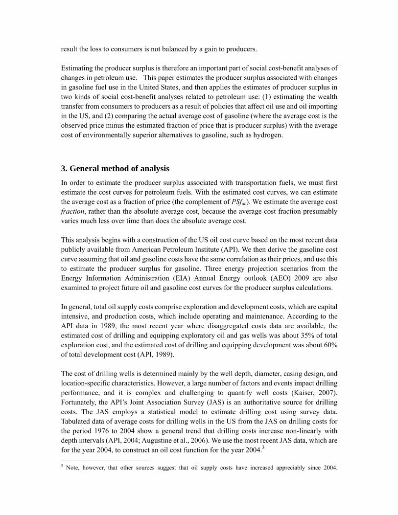
5.1.4 Total oil cost curve

The sum of all the costs incurred to oil supply yields the total oil cost curve shown in Figure 5. Table 3 summarizes the data source and method to estimate each cost component. Total US oil production (Q0) including lease condensate in 2004 was 5.419 MMBD and the oil price P0 was $38/bbl (crude oil domestic first purchase price) (EIA, 2009b). According to our estimated oil cost curve MC(Q), the corresponding marginal cost was $28.85/bbl. This divergence between price and marginal cost is due most likely to world oil market not being perfectly competitive (on account of occasional oligopolistic behavior), although it is possible that we have omitted some costs. The US oil producer surplus fraction (PSf) of total prices-times-quantity payments in 2004 is about 70%, calculated using the following:

PSf 1MC(Q)dQ

0

Q0P0 *Q0

(8)

where MC(Q)is the marginal cost of oil for the US in 2004:

Oil marginal cost = Exploration + development + “other costs” + production (9)

and the complete function form is as follows:

)exp()exp()exp()( 2211 oilOEDoiloiloiloil QdcCQbaQbaQMC

The parameters a1, b1, a2 and b2 are estimated in 2 specification (3) of Table 2. The average oil cost is $11.29/bbl, calculated with the integral of the marginal cost curve from 0 to 5.419 MMBD divided by the oil production.

Figure 5. US oil cost curve in 2004

US oil marginal cost curve (2004)

MC=$28.85/bbl

Q0=5.419

P0=$38/bbl

0

10

20

30

40

50

0 1 2 3 4 5 6 7Oil Production (MMBD)

200

5 $/

bbl

ProducerSurplus (PS)

MC

Table 3. Summary of each cost component in 2004 oil marginal cost function Cost

component

Data source Model/Method

Exploration

(MEC)

JAS/API (API, 2004)

for oil wells

MEC=exp(a1+b1Q)

Development

(MDC)

JAS/API (API, 2004)

for oil wells

MDC=exp(a2+b2Q)

Other costs

(OED)

FRS/EIA (EIA,

2008a) for oil and gas

wells for 2003-2004

Compare historical data 1977-1982 from FRS (EIA, 2008a) and

API (API, 1989), scale FRS cost with the ratio API/FRS, and

assume average OED is independent of oil output

Production

(MPC)

FRS/EIA (EIA,

2008a) for oil and gas

wells for 2003-2004

Scale FRS cost with the ratio API/FRS; Assume MPC is an

exponential function of output MPC c exp(d Q), justified

by US Economic Census on oil and gas operations.

Ideally, we would estimate the oil cost curves for OPEC and ROW separately using a similar method. However, the API JAS data does not include detailed drilling cost data for other regions. Although the FRS data contains total oil costs for other foreign regions, including Canada, OECD Europe, Africa, Middle East, FSU & East Europe, and other Western and Eastern Hemispheres, the cost data were incomplete for some regions and expenditures on oil wells and gas wells were not distinguishable. Furthermore, FRS covers major energy-producing companies only. We therefore treat OPEC and ROW differently, using data from the World Bank (Section 5.3). 5.2 Current US gasoline cost curve

The objective in this section is to estimate the marginal wholesale cost of producing gasoline from US crude oil, compare that with the price of gasoline, and estimate the associated total producer surplus, for the refining industry and the oil industry. Because we already have estimated the marginal cost of producing crude oil in the US, and we know that the marginal cost of gasoline (MCg) is related to the marginal cost of oil (MCo), we will derive a simple linear relationship where the marginal cost of gasoline at the refinery gate is equal to the marginal cost of refining (in dollars per gallon of gasoline, or $/gg) plus the marginal cost of the oil input to the refinery (expressed in $/gg). This relationship will have the form:

MCg k1 k2 MCo (10)

where MCg is the marginal wholesale cost of gasoline at the refinery gate in $/gg, k1 is the constant marginal cost of refining in $/gg (assumed to be independent of the cost and quantity of oil refined), MCo is the marginal cost of oil in dollars per barrel of crude oil produced ($/bcp) (Equation 7), and k2 is a coefficient that converts the cost of oil production in $/bcp to the contribution of oil cost to the marginal wholesale gasoline cost in $/gg; hence, k2 has units

($/gg)/($/bcp). Note that we do not estimate the marginal cost of downstream gasoline marketing (gasoline transportation and gasoline retailing), because we believe that producer surplus in downstream marketing is relatively small, on account of the strong competition and similar cost structures among marketing firms. To derive the expression for MCg in Equation 10, we first set up the following analogous linear relationship between the price of gasoline and the price of crude oil, which we can estimate on the basis of historical data (see Figure 6):

Pg a b Po (11)

Pg ($/gg) is what the Energy Information Administration (EIA) calls the “refiner sales price to resellers.” Refiner sales prices to resellers are pre-tax wholesale prices for sales of motor gasoline to purchasers who are other than ultimate consumers (Table 5.22 of EIA, 2009b). These are thus wholesale prices at the refinery gate and presumably exclude downstream marketing price margins (transportation and retailing) as well as taxes. Po ($/bcp) is the “crude oil domestic first purchase price” (Table 5.18 of EIA, 2009b), which according to the EIA’s glossary (EIA, 2009b) is “the price for domestic crude oil reported by the company that owns the crude oil the first time it is removed from the lease boundary.” The basis of this price thus appears to be the same as the basis of our estimates of the marginal cost of oil production (Equation 7). a is a constant in $/gg (year 2005 $) and is what the EIA (2009b) calls the “refiner margin” for motor gasoline. The refiner margin is the difference between the price to resellers (Pg here) and what the EIA (2009b) calls the “crude oil refiner acquisition cost” expressed in $/gg. The crude oil refiner acquisition cost expressed in this way is essentially the contribution of the oil price to the wholesale refinery-gate price of gasoline. We define the term b.Po in Equation 9 so that it is this contribution of the oil price to the wholesale gasoline price (see explanation of b, next).7 b is a conversion coefficient: the ratio of the contribution of the crude oil price to wholesale gasoline price, in $/gg, to the price of crude oil produced, in $/bcp. We estimate the parameters a and b in two ways. In the first method, we estimate a as the refiner margin reported by the EIA (Table 5.22 of EIA, 2009b), and estimate b by dividing the contribution of the crude oil price to wholesale gasoline price by Po (Table 5.18 of EIA, 2009b). The contribution of crude oil price to wholesale gasoline price is calculated as the difference between Pg (Table 5.22 of EIA, 2009b) and the refiner margin for motor gasoline (Table 5.22 of EIA, 2009b). In the second method, we regress Pg on Po (Table 5.18 of EIA, 2009b). The results of both methods are given in Table 4. All prices in are in constant 2005 US dollars.

7 The EIA also reports the actual refiner crude oil acquisition cost in $/bbl, and presumably uses this to calculate the contribution of oil price to gasoline price, in $/gg. The difference between the crude oil refiner acquisition cost in $/bbl and the crude oil domestic first purchase price (Po in Equation 8) is that the former includes some minor additional transportation and “other” fees, which typically are on the order of $3/bbl (our estimate by comparing Table 5.18 with Table 5.21 in EIA, 2009b). However this difference is not relevant to our calculation because we use the coefficient b to convert Po into the contribution of oil price to the wholesale gasoline price.

Table 4. Results of constant a and coefficient b

a b a=Refiner margin b=oil/gasoline ratio

0.343 0.0250 Average 1993-2009 0.389 0.0244 Average 2000-2009 0.422 0.0239 Value in 2004

Regress Pg on Po (1993-2009 data) 0.320 *** 0.0257 *** Unadjusted R-squared = 0.985 (0.0319) (0.0008)

Regress Pg on Po (2000-2009 data) 0.368 *** 0.0249 *** Unadjusted R-squared = 0.975 (0.0699) (0.0014)

Notes: Standard errors in parentheses. Significance codes: * 5% level, ** 1% level, and *** 0.1% level.

The two methods give similar estimates of a and b. The estimates of a (the refiner margin) differ by only 5-7%, and the estimates of b (the $/gg/$/bcp coefficient) differ only by 2-3%. We will use the regression for the more recent period, 2000 to 2009; hence, a = 0.368 and b = 0.0249.

Figure 6. Crude oil domestic first purchase price and motor gasoline refiner sales prices to resellers

Crude oil and gasoline prices over time

0102030405060708090

100

1991 1996 2001 2006 2011

Year

2005

$/bc

p

0

0.5

1

1.5

2

2.5

3

2005

$/gg

Oil prices

Gasoline prices

The next step is to derive an expression for marginal cost from Equation 11. We know that the price is equal to the marginal cost plus producer surplus, so we can split all of the price terms of Equation 11, including the constant a, into MC and producer surplus components:

Pg MCg PSg a MCfg,r a 1MCfg,r b MCo PSo a MCfg,r a 1MCfg,r b MCo b PSo

(12)

where producer surplus is producer surplus and MCfg,r is the marginal cost fraction of the price constant for gasoline refining. Next, we separate the MC and producer surplus terms:

,

,

(13)

1 (14)

g g r o

g g r o

MC a MCf b MC

PS a MCf b PS

Note that Equation 13 has the same form as Equation 10. Next, we substitute the Equation 9 expression for MCo into the MCo term of Equation 13:

MCg a MCfg,r b [exp(a1 b1 Qo ) exp(a2 b2 Qo )COED c exp(d Qo )] (15)

Thus far we have estimated all of the terms except MCFg,r, the marginal cost fraction of the refiner margin for gasoline. We assume MCFg,r, = 0.80 according to the average ratio of petroleum product net refining margin to petroleum product gross refining margin from 1988 to 2009 with data from EIA Financial Reporting System. The gasoline marginal cost curve estimated by Equation 15 is shown in Figure 7. The next step is to find the price and quantity lines for gasoline production from domestic crude oil in our reference year of 2004. According to the EIA (2009b), in 2004 the refiner “sales price to resellers” for motor gasoline – the same price basis used for Equation 11 and Figure 6 – was $1.29/gallon in nominal dollars and $1.33 in year 2005 dollars. Because our objective here is to estimate the marginal cost of producing gasoline from US crude oil, in US refineries, the relevant total quantity is the amount of gasoline that would have been produced had all domestically produced crude oil in 2004 been input to refineries, which is equal to Qo,2004 (5.419 MMBD) multiplied by the ratio of actual motor-gasoline produced by refineries to crude oil input to refineries in 2004 (EIA, 2009b), resulting in 122 mmgd. The producer surplus associated with domestic gasoline fuel made from domestic crude oil is the area bounded by price line and marginal cost curve from output level zero to the estimated 122 mmgd gasoline output in 2004 from domestic oil.

Figure 7. Marginal Cost of producing gasoline from US crude oil in 2004

Gasoline marginal cost curve in 2004

Pg=$1.33/gal

-0.10.10.30.50.70.91.11.31.5

0 20 40 60 80 100 120 140

Million gallons per day

2005

$/g

al

MCPS

Qg=122M gal

PS1

PS2

The calculated producer surplus is about 56.7% of total price-times-quantity payments, which includes both domestic oil production and refinery industries. This producer surplus fraction is lower than that oil producer surplus fraction (70% from Figure 5), which follows from our assumption about the producer-surplus fraction for refining (1-MCFg,r, Equation 14). We may break the producer surplus into two components: one related to the steepness of the cost curve (the area PS2, about 58%), and the other related to the price being higher than it should be (the area PS1, about 42%) due to the scaling up of oil price/MC gap (our assumption to derive gasoline cost). PS1 is the rectangle area below the gasoline price and above the marginal cost $1.01/gal) at Qg, and PS2 is the area below the marginal cost $1.01/gal) and above the marginal cost curve. In the terms of Table A1, PS1 is economic profit, and PS2 is economic rent. If our estimate of the cost curve is accurate, then the petroleum-refining industry is not competitive, and receives economic profit (PS1 in Figure 7). However, it is possible we have under-estimated costs and that there is no economic profit (PS1=0). The area under the gasoline cost supply (total gasoline cost) is about $69.96 million per day while the area under the oil cost curve in Figure 5 (total oil cost) is about $61.17 million per day (about 53.4% is for gasoline). To estimate the producer surplus in the refining industry only, we assume that the revenue to the refining industry is the revenue difference between gasoline and oil, and the cost to the refining industry is the cost difference between gasoline and oil. We calculate the producer surplus fraction in the refining industry is about 28%, much lower than that in the oil industry. 5.3 Producer surplus as a function of the change in gasoline consumption

In the previous section we estimated the total producer surplus for gasoline that could have been produced from domestic crude oil in 2004. In this section we estimate producer surplus as a function of the size of the change in gasoline consumption. We estimate the total producer

surplus change for the change in consumption (we designate this ∆PSt, where t stands for “transfer”), and producer surplus as a fraction of the change in price-times-quantity payments (we designate this PSfac, where ac stands for “average cost”). △PSt is calculated with the following equation:

])()[(])()[(*0

0

**

0

00 gg Q

gggg

Q

ggggt dQQMCQPdQQMCQPPS , (16)

where Pg0 = the before-change gasoline price, Pg

*= the after-change gasoline price, Qg0= the

before-change gasoline quantity, Qg* = the after-change gasoline quantity at the new

equilibrium (shown in Figure 8), and MC(Qg )= marginal cost function of gasoline MCg . We

break the total producer surplus change (PSt ) into two pieces: one (we call this component △

PSt,c, which is the triangular area ABC) is due to the equilibrium consumption change and the second component (called △PSt,i, which is the rectangular area BCP0P*) is due to the change in price (“inframarginal” consumption), shown in Figure 8 and estimated in the following equations:

PSt PSt,c PSt,i (17)

PSt,c [(Pg0 Qg

0 ) MC(Qg )dQg0

Qg0

][(Pg0 Qg

*) MC(Qg )dQg ]0

Qg*

(18)

PSt,i (Pg0 Pg

*) Qg* . (19)

The only unknown is the after-change gasoline price Pg* . To estimate this, we employ the oil

demand function used in NEMS (EIA, 2010), shown in Equation 20:

Qd Pd , (20)

where P is the price, Qd is the demand quantity, d = -0.11 is the demand elasticity from NEMS (EIA, 2010), and is a constant to be determined by a point on the curve. We assume that the US oil market is competitive. Given this, Figure 8 (D = demand) illustrates two supply-demand equilibrium cases before and after oil demand contracts, where MC (cost curve S) has the same shape as we estimate for 2004 (Figure 5), but vertically shifts up so that the curve passes through the point (P0, Q0), and intersects the original demand curve D at A. When oil demand declines from Q0 to Q,’ the new demand curve D’ will pass through point N (P0, Q

’), but with the same demand elasticity as the initial demand curve D.

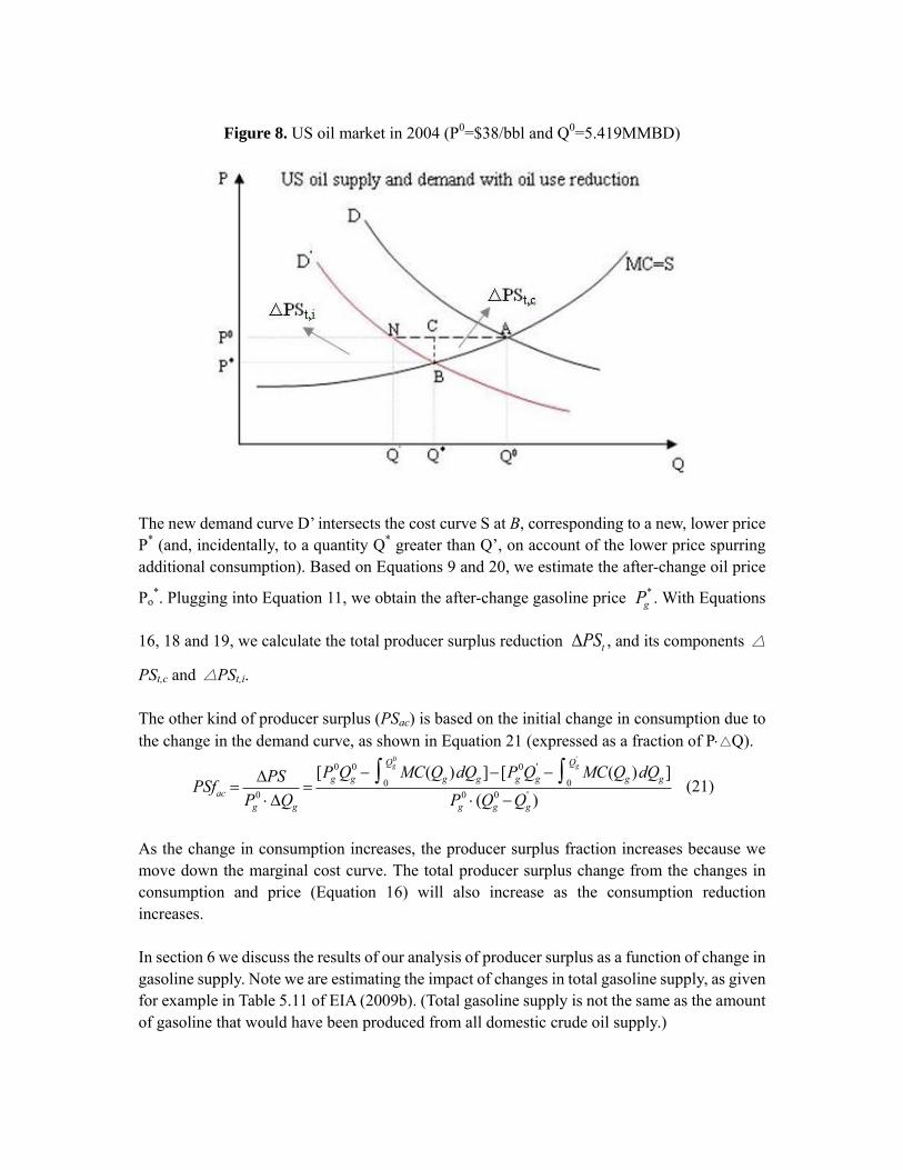
Figure 8. US oil market in 2004 (P0=$38/bbl and Q0=5.419MMBD)

The new demand curve D’ intersects the cost curve S at B, corresponding to a new, lower price P* (and, incidentally, to a quantity Q* greater than Q’, on account of the lower price spurring additional consumption). Based on Equations 9 and 20, we estimate the after-change oil price

Po*. Plugging into Equation 11, we obtain the after-change gasoline price Pg

* . With Equations

16, 18 and 19, we calculate the total producer surplus reduction PSt , and its components △

PSt,c and △PSt,i. The other kind of producer surplus (PSac) is based on the initial change in consumption due to the change in the demand curve, as shown in Equation 21 (expressed as a fraction of P△Q).

PSfac PS

Pg0 Qg

[Pg

0Qg0 MC(Qg )dQg0

Qg0

][Pg0Qg

' MC(Qg )dQg0

Qg'

]

Pg0 (Qg

0 Qg' )

(21)

As the change in consumption increases, the producer surplus fraction increases because we move down the marginal cost curve. The total producer surplus change from the changes in consumption and price (Equation 16) will also increase as the consumption reduction increases. In section 6 we discuss the results of our analysis of producer surplus as a function of change in gasoline supply. Note we are estimating the impact of changes in total gasoline supply, as given for example in Table 5.11 of EIA (2009b). (Total gasoline supply is not the same as the amount of gasoline that would have been produced from all domestic crude oil supply.)

5.4 Estimating producer surplus for OPEC and the rest of the world

To estimate producer surplus for OPEC and the rest of the world, we start with unpublished World Bank data on crude oil annual average world price and production in years 2003 and 2004 to develop oil supply cost curves for OPEC and ROW (the Rest of the World except the US). The World Bank data contains annual oil production, rent (total revenue minus total cost8, i.e. total producer surplus) and average world price for many countries from 1970 to 2004, including ten OPEC members (Iraq, Iran, Kuwait, Sandi Arabia, Venezuela, Qatar, Indonesia, United Arab Emirates, Algeria and Nigeria). We assume an exponential function form with two parameters similar to Equation 5 for OPEC and ROW marginal cost curves. One country’s total oil cost for each year is calculated with the world oil price times the country’s oil output minus the country’s oil rent.9 The sum of total oil costs for the ten OPEC members gives the total OPEC oil cost and the sum of total oil costs for the rest of the countries (except the US) gives the total ROW oil cost. We calibrate the exponential curve with the most recent data (years 2003 and 2004) for OPEC and ROW separately, and then obtain the following functions:10

)*00084.0exp(*819.2 OPECOPEC QMC (22)

)*0006.0exp(*433.9 ROWROW QMC , (23)

where Q is in billion barrels and MC is in constant 2005 US dollars per barrel. The oil marginal cost curves for OPEC and ROW in 2004 are shown in Figure 9. The oil marginal cost for OPEC is less than one-third of that for ROW. It appears that the two curves are linear because the exponents in the Equations 13 and 14 are close to zero. We provide two more detailed view graphs for OPEC and ROW but with different y-axes. The ROW curve shows decreasing marginal cost, which may be wrong because the World Bank data has some missing values for some regions. Compared to the US oil cost curve in Figure 5, OPEC has a much lower marginal cost and the cost increase with output level is very little, i.e. the marginal oil cost of OPEC is quite inelastic with respect to its output. According to the World Bank data, OPEC oil output in 2004 was about 25.3 MMBD with average cost of $2.9/bbl and ROW oil output in 2004 was about 37.4 MMBD with average cost of $9.3/bbl. In contrast, our estimate for the corresponding marginal cost is $2.84/bbl for OPEC with Equation 13 and $9.36/bbl for ROW with Equation 14. Given the world oil price at $38/bbl in 2004, OPEC earns a large amount of producer surplus. To shed some light on the foreign producer surplus, this paper provides some rough calculations of producer surplus from OPEC and ROW in 2004 as compared to the US results.

8 Unfortunately, the World Bank data does not provide the definition of rent. We treat it as the difference between revenue (price times oil output) and total cost. As the World Bank data includes the US, we compare the calculated average oil cost ($11.86/bbl) to our estimate ($11.29/bbl) for 2004 and they are very close. 9 Here the oil rent is defined as the product of oil output and the difference between oil price and average oil cost, same as the definition of total producer surplus. This is different from the economic rent discussed in Section 2. 10 The calibration method is the same as our estimate for US oil production marginal cost (MPC) in Section 5.1.

Figure 9. Oil supply cost curves for OPEC and ROW

Estimated oil cost curves for OPEC and ROW in 2004

0

2

4

6

8

10

0 5 10 15 20 25 30 35 40

Oil production (MMBD)

2005

$/b

bl

OPEC ROW

OPEC oil MC curve (2004)

2.815

2.82

2.825

2.83

2.835

2.84

2.845

0 5 10 15 20 25 30

Oil production (MMBD)

2005

$/b

bl

ROW oil MC curve (2004)

9.34

9.36

9.38

9.4

9.42

9.44

0 5 10 15 20 25 30 35 40

Oil production (MMBD)

2005

$/b

bl

Given the 2004 oil price P0 ($38/bbl), the oil producer surplus fraction of total price-times-quantity payments is about 92.5% for OPEC and about 75.5% for ROW as shown in Figure 10 (shaded areas). This amounts to $35/bbl for OPEC and $29/bbl for ROW. By contrast, the US oil producer surplus fraction in 2004 is about 70% (Figure 5) and $27/bbl. Comparing magnitudes, the total OPEC producer surplus associated with total OPEC production in 2004 (25.3 MMBD) is $325 billion, which is more than six times the total US producer surplus associated with total US oil production (5.419 MMBD), about $53 billion. In 2004, OPEC oil production is more than 4 times US oil production. According to the recent data from EIA FRS (EIA, 2008a), total cost (acquisition, exploration, development and production) incurred for petroleum operations increased sharply from 2004 to 2008 for the US and foreign producers. Particularly, the 2008 petroleum expenditure in the Middle East is about 3.2 times the 2004 one in real dollars, and oil price rose from $38/bbl to $86.69/bbl in 2005 dollars. We can make some rudimentary projections of producer surplus fraction for 2008,

which we project to be about 92%.

Figure 10. Oil producer surplus calculation for OPEC and ROW

OPEC oil MC curve (2004)

38

25.2905

10152025303540

0 5 10 15 20 25 30

Production (MMBD)

2005

$/b

bl

ROW oil MC curve (2004)

38

37.405

10152025303540

0 5 10 15 20 25 30 35 40Production (MMBD)

2005

$/b

bl

With the estimated producer surplus to the US refinery only in section 5.2, we can estimate the total gasoline producer surplus fraction with imported oil from OPEC or ROW. Table 5 summarizes all the producer surplus fractions in 2004 for oil industry in the US, OPEC and ROW, for US refinery industry, and for the total gasoline cost given three different combinations (US oil + US refining, OPEC oil + US refining, and ROW oil + US refining). We assume actual total oil inputs and gasoline outputs in 2004, but with different sources for the oil input. For the US, the total gasoline producer surplus fraction for imported oil would be higher than that for domestic oil.

Table 5. Summary of all the producer surplus fractions in 2004, for total production

Oil industry US 70.3% $27/bbl

OPEC 92.5% $35/bbl

ROW 75.5% $29/bbl

US refinery US 27.9% $0.12/gal ($5/bbl)

Total gasoline in US

(oil + refinery)

US oil + US refinery 56.7% $0.75/gal ($32/bbl)

OPEC oil + US refinery 71.8% $0.96/gal ($40/bbl)

ROW oil + US refinery 60.5% $0.80/gal ($34/bbl)

How much would producer surplus decrease with a 10% contraction of world oil demand? We first calculate the percentage change in world quantity resulting from an assumed percentage change in world demand, and then assume that the calculated percentage change in world quantity applied to OPEC, ROW, and US To answer the question, we should first estimate the world oil price P* after the oil demand change, which depends on our view of the world oil market. If we assume it is a competitive world market, then P* equals marginal cost (MC*) where the MC* at Q* (quantity after the change) is determined by the “world” long-run marginal cost function. If we assume that OPEC simply maintains price, then P* equals P0. Any assumptions between MC* and P0 are possible. We derive the “world” oil cost curve including the US shown in Figure 11 with the World Bank data using the same method as the OPEC and ROW oil cost curves in this section. Our derived hypothetical “world” marginal cost, which depicts world short-run cost curve in 2004, is given by:

)*000034.0exp(*7123 worldworld QMC . (24)

The “world” oil marginal cost is about $7.13/bbl, much lower than world oil price P0. If the “world” oil cost curve is believable to some extent, then we can conclude that the world oil market is not perfectly competitive, most likely due to OPEC behavior. To formally model OPEC behavior is beyond the scope of this paper, and will be addressed in the future research. As the 2004 “world” oil MC curve is almost flat, we assume that oil demand contraction would result in the same percentage change in world quantity.

Figure 11. “World” oil cost curve

"World" oil MC curve (2004)

7.122

7.123

7.124

7.125

7.126

7.127

7.128

7.129

7.13

0 10 20 30 40 50 60 70

Oil Production (MMBD)

2005

$/bb

l

Table 6 presents the result of two different kinds of producer surplus change for 10%, 20% and 50% oil-demand contractions under three scenarios of OPEC pricing behavior, in order to examine the sensitivity to P* and therefore to assumptions about OPEC market power. The range of cases (scenarios) we examine spans perfect competition to full OPEC market power. For case 1, P*=MC* (this is not likely according to the World Bank data); for case 2, P*= the mean of P0 and MC* we call this P1); for case 3, P*=P0, the same price as before the demand contraction (assuming in this case that OPEC’s strategy is to maintain oil price). Under case 1, for a 10% contraction in demand for oil, the total producer surplus reduction △PSt (289.5 billion$) for OPEC expressed as $/bbl (△PSt/△Q) is $312.8/bbl where △PSt,c per barrel is $34.9, and △PSt,i per barrel is $277.8. OPEC’s producer surplus fraction PSfac for the 10% demand contraction is 91.9%. As the oil demand contraction increases, the total producer surplus

reduction will increase and △PSt,c per barrel will increase slightly, but △PSt,i per barrel will decline. For ROW and US, P* is lower than their marginal cost and they would not produce crude oil. As shown in Table 6, for case 2, △PSt,c per barrel increases slightly while △PSt,i decreases sharply with increasing contraction of oil demand for both OPEC and US However, for ROW, △PSt,c per barrel declines as oil-demand contraction increases due to decreasing marginal cost curve (Equation 14). As shown by Equation 10c, the $/bbl change in △ PSt,i, the “inframarginal” producer surplus, is proportional to the change in price: the greater the change in price, the greater the $/bbl reduction in producer surplus on the inframarginal consumption. If there is no change in price, then △PSt,i is zero (case 3 of Table 6). There will be no change in price if, after the initial contraction of demand, OPEC reduces its output so that the amount of high-cost supply forced into the market raises the price back to the original, pre-contraction level. Whether OPEC would actually do this in the face of a demand contraction depends on the details of its short-run and long-run objective functions. OPEC’s short-run strategy is to maximize producer surplus by finding the optimal output that maximizes their revenue, when the benefit from the higher price no longer more than compensates for the reduced sales. OPEC’S long-run strategy is more complicated as they do not want to maintain high prices for so long that consuming countries begin to take long-run oil conservation measures. Both of these strategies are difficult to model, even for OPEC itself, and as a result we offer only scenarios, rather than predictions. For cases 2 and 3, OPEC has more producer surplus reduction per barrel than ROW which in turn has more producer surplus reduction than does the US. Therefore, oil consumption contraction would have more impact on foreign producers than on US producers.

Table 6. Oil producer surplus changes after 10%, 20% and 50% contractions of world oil demand under three price-response cases.

Case 1 (P*=MC*)

Contraction of world oil

demand

Quantity reduction

apportioned to:

△PSt ($/bbl) △PSt ($ billion)

PSfac

△PSt,c △PSt,i

10% P*=$7.13/bbl OPEC 34.93 277.83 -289.5 91.9%

ROW - - -

US - - - 20% P*=$7.13/bbl

OPEC 35.05 123.48 -293.5 92.2%

ROW - - - US - - -

50% P*=$7.13/bbl

OPEC 35.12 30.87 -305.4 92.4% ROW - - -

US - - -

Case 2 (P*=mean(P0, MC*)) Case 3 (P*=P0=$38/bbl)

Contraction of world oil

demand

Quantity reduction

apportioned to:

△PSt ($/bbl) △PSt ($ billion)

PSfac △PSt ($/bbl) △PSt ($ billion)

PSfac

△PSt,c △PSt,i △PSt,c △PSt,i

10% P*=$22.57/bbl P*=$38/bbl

OPEC 34.93 138.92 -160.9 91.9% 34.93 0 -32.3 91.9%

ROW 29.39 138.92 -230.6 77.3% 29.39 0 -40.3 77.3%

US 13.44 138.92 -27.6 35.4% 13.44 0 -7.3 35.4%

20% P*=$22.57/bbl P*=$38/bbl

OPEC 35.05 61.74 -179.2 92.2% 35.05 0 -64.9 92.2%

ROW 29.01 61.74 -248.7 76.3% 29.01 0 -79.5 76.3%

US 16.69 61.74 -85.0 43.9% 16.69 0 -18.1 43.9%

50% P*=$22.57/bbl P*=$38/bbl

OPEC 35.12 15.44 -234.0 92.4% 35.12 0 -162.5 92.4%

ROW 28.77 15.44 -302.9 75.7% 28.77 0 -197.1 75.7%

US 22.60 15.44 -103.1 59.5% 22.60 0 -61.2 59.5%

5.5. Future Oil and Gasoline Marginal Cost 5.5.1. Overview of the estimation method In this section, we estimate the future oil marginal cost curve and then the future gasoline marginal cost for the US based on historical data and our estimated 2004 US oil marginal cost curve. In general, the cost of oil in the US in the future can be influenced by geopolitics, technological progress, oil output, world oil price, remaining reserves, investors’ strategy, alternative energy options, and other factors. Here we model the future annual total cost (TC) in billion dollars of petroleum from both oil and gas wells (the API and the EIA FRS do not provide cost data for oil wells and gas wells separately) as a function of time (t), oil price (Poil), oil output (Qoil), gas output (Qgas) and remaining reserves (Rev) of oil and gas (Equation 25):

)Re,,,( , vQQPtfTC gasoiloil (25)

We fit the historical cost data from API and EIA FRS, and choose the best-fitting one among different functional forms for estimations. Assuming oil and gas production have the same average cost (in dollars per barrel), we then estimate the average oil cost in the future through 2030 by dividing the estimated total cost TC by total oil and gas production. To obtain the future oil marginal cost curve, we shift the 2004 US oil cost curve so that the curve produces the same average oil cost as we estimate. Finally, gasoline marginal cost curves are derived from oil cost curves using the method in section 5.2. 5.5.2. Detailed estimation method

The EIA AEO 2009 (EIA, 2009a) projects US oil and gas supply, demand, prices and end of year reserves through 2030 under five cases: reference, high price, low price, high economic growth and low economic growth. The lower 48 crude oil wellhead price in 2030 is projected to be $45/bbl under low price case (oil output: 5.36 MMBD) and $194/bbl under high price case (oil output: 8.47 MMBD). The total cost incurred to extract and produce petroleum sources includes expenditures on acquisition, exploration, development and production. The historical total cost data from API and EIA FRS for the period from 1977 to 1991 indicates that the FRS total cost was about 70% of the API total cost. We extrapolate the API total cost by dividing the FRS total cost by 0.7 for the years 1991 to 2007. Thus we have total cost (TC) available over years 1977 to 2007. The time variable t is defined as the year minus 1975. For each case in EIA AEO 2009 (e.g., reference case, low-price case), a new variable “Price Difference” is generated by the annual oil price (EIA, 2009a, Greene and Tishchishyna, 2009) minus the average oil price over the years 1977-2030. The variable “Price Difference” is labeled as “Pdiff” under the updated reference case, “PdHP” under the high-price case, “PdLP” under the low-price case, “PdH” under the high-economic growth case, and “PdL” under the low-economic growth case. Historical oil output and gas output are from EIA (EIA, 2008b) and projected ones are from EIA AEO 2009 (EIA, 2009a). Remaining oil and gas reserves (beginning-of-year) in 2007 are estimated by adding the 2007 oil and gas production to the 2007 end-of-year oil & gas reserves (billion barrels) (EIA, 2008b). For the period from 1977 to 2006, the beginning-of-year reserves are calculated backward. We take the natural logarithm of the total cost TC as the dependent variable and try different combinations of the five variables (time, oil production, gas production, price difference and natural logarithm of reserves) as regressors. Regression results show that coefficients on oil production and price difference are statistically significant at 5% level and the coefficient on gas production is not statistically significant even at 25% level. Based on this, we may assume that changes in total cost over time are independent of changes in gas production (we assume that gas cost is included in the constant in the total cost function). In theory, TC should decrease with time (because technology improves over time), increase with annual oil output (supply Qoil), and increase with decreasing reserves (because remaining reserves are increasingly costly to access). We exclude results that are inconsistent with these theoretical expectations and finally choose oil output and price difference as two dependent variables for regression of total

cost under the five cases shown in Table 7. The coefficients on oil output and price difference and the R-squared values are the same across the five cases; only the constants differ. Given this, it does not matter which case we use. For convenience we use the Reference oil price case. Table 7. Regression of natural logarithm of total cost on oil output and price difference (using data from 1977 to 2007)

Ln(tc) Coefficient Std Error Reference (Ref)

Const 4.636 *** 0.197 Qoil  0.061 *  0.025 Pdiff  0.028 *** 0.002 R-squared = 0.861

High-price (HP)

Const 5.351 0.225 Qoil  0.061 0.025 PdHP  0.028  0.002 R-squared = 0.861

Low-price (LP)

Const 4.083 *** 0.184 Qoil  0.061 *  0.025 PdLP  0.028 ***  0.002 R-squared = 0.861

High-Econ (HEN)

Const 4.749 *** 0.201 Qoil  0.061 *  0.025 PdH  0.028 ***  0.002 R-squared = 0.861

Low-Econ (LEN)

Const 4.670 *** 0.198 Qoil  0.061 *  0.025 PdL  0.028  0.002 R-squared = 0.861

Notes: Standard errors in parentheses. Significance codes: * 5% level, ** 1% level, and *** 0.1% level. The functional form of total cost for the reference oil price case is given by:

)028.0061.064.4exp( PdiffQTC oil (26)

Figure 12 shows the predicted (fitted) versus historical total cost against time for the reference case. The regression appears to reflect the general trend of total cost.

Figure 12. Estimated vs. actual total costs ($/year)

TC estimated vs. historical

0

50

100

150

200

250

1975 1980 1985 1990 1995 2000 2005 2010

Year

2005

$ b

illi

o

Historical Estimated (Ref)

To estimate the average cost beyond 2007, we assume that oil average cost is the same as gas average cost and divide predicted total annual cost beyond 2007 by total annual oil and gas output. We predict future total cost using Equation 26 and the EIA’s Ref, LP, HEN, and LEN oil price projection cases. We do not use the EIA’s high oil price case (HP) because it entails increased production from onshore CO2–enhanced oil recovery projects and offshore deepwater projects, and these sources have a cost structure different than that of the historical mix of sources upon which our regression is built. High oil price would also encourage unconventional oil development, which is beyond of the scope of our analysis. Moreover, our regression results for the high-price case are not realistic: the projected average oil cost beyond 2015 is over $200/bbl, which is even higher than EIA projected price (AEO 2009 high price case). The predicted future average cost, shown in Figure 13, closely follows the EIA’s AEO 2009 reference case projection of oil prices.

Figure 13. Our Projected oil average costs and EIA projected oil prices

Our predicted (fitted) average cost over time (Reference)

$-

$20.00

$40.00

$60.00

$80.00

$100.00

$120.00

2005 2010 2015 2020 2025 2030 2035

Year

2005

$/b

b

Our predicted average cost EIA projected prices (AEO 2009 reference) Time-average average cost

To estimate the marginal cost curve for any future year, we vertically shift the 2004 oil marginal cost curve (Figure 5) such that the shifted curve generates the same average cost in that particular year, where the average cost is the integral of the oil cost curve from oil output zero to the EIA projected oil production, divided by the projected oil production. Formally:

SMCMC f 2004 , (27)

where fMC = future oil marginal cost, 2004MC = the 2004 oil marginal cost (equation 7) and

were S = shifter (constant value) is given by:

f

Q

ff

Q

dQMCQACS

f

0 2004

. (28)

This method assumes that the US oil industry employs the current recovery technology in the future. To present a general trend of future oil marginal cost curve instead of a curve for each

years, we take the average oil average cost ( fAC ) for the period 2005-2030 as a proxy for

estimating a single future oil marginal cost curve. The corresponding future oil production ( fQ )

is just the time-average one (5.92 MMBD for the reference case). The derived US future oil marginal cost curves for the four EIA oil-price cases (all except HP) are shown in Figure 14, as compared with the 2004 curve (Figure 5). As shown in Figure 14, the estimated future curve for the low-price case (LP) is not reasonable, and the other three curves are almost the same (about $30/bbl more than the 2004 value). Therefore we analyze the reference case only in this paper.

In the final step, we use the method of section 5.2 to derive the gasoline marginal cost curve from the oil marginal cost curve derived above. We regress gasoline price on oil price and a constant using the EIA projections from 2005 to 2030 for the reference case (EIA, 2009a). To derive the gasoline cost curves, we assume MCFg,r, = 0.85 because US refineries have shown decreasing net margins in recent years. Figure 15 shows the estimated future gasoline cost curve in the US Using the same conversion factor (the ratio of actual motor-gasoline produced by refineries to crude oil input to refineries in 2004) as in Section 5.2, we estimate the future gasoline production (132.80 million gallons per day) that refineries would produce if they used all and only domestic crude oil. The results of this analysis are discussed in section 6.2.

Figure 14. Current and Predicted future oil marginal cost curves

Future oil marginal cost curve (US)

-50

0

50

100

150

200

250

0 1 2 3 4 5 6 7 8 9

Oil production (MMBD)

2005

$/b

blFuture (Ref)

2004

Future (HEN)

Future (LEN)

Future (LP)

Figure 15. Estimated gasoline marginal cost curve

Estimated Future Gasoline Marginal Cost Curve (US reference case)

Pg=$2.75/gal

Qg

0

0.5

1

1.5

2

2.5

3

0 20 40 60 80 100 120 140

Gasoline Production (Million gallons per day)

2005 $/gal

Producer Surplus MC

6. Results

6.1 Analysis of producer surplus as a function of change in total gasoline supply in the US in 2004

We calculate the percentage change in total gasoline supply11 associated with the assumed percentage contraction of demand, then assume that this percentage change in quantity applies to supply from US, OPEC and ROW. Then we calculate the producer surplus changes for gasoline made in US from US crude oil, OPEC crude oil and ROW crude oil respectively. For 10%, 20%, 50% and 100% contractions of demand for motor gasoline in the US in 2004, the calculated percentage changes in total gasoline supply are 7.06%, 14.36%, 38.21% and 100%, respectively. According to EIA Annual Energy Review (EIA, 2009b) and Transportation Energy Data Book (EIA, 2011), the total gasoline supply in 2004 was 9.105 MMBD, 65% crude oil was imported, and among total imports, OPEC share was 43.4%. Given this, then 3.18 MMBD gasoline supply was from US oil, 2.57 MMBD from OPEC oil, and 3.35

11 We employ the same functional form as equation 10 for total gasoline supply and demand curves. The total gasoline supply elasticity is set as 0.25 and demand elasticity is -0.11 as used in NEMS (EIA, 2010b).

MMBD from ROW oil. Table 8 presents the producer surplus changes (△PSt in $ billion including △PSt,c and △PSt,i, and PSfac) for 10%, 20%, 50%, and 100% contractions of demand for motor gasoline in the US Because △PSt,c is the producer surplus associated with the foregone gasoline use, it always increases with increasing percentage reductions in gasoline use. The △PSt,c in terms of $/gal is constant for gasoline made in US from OPEC and ROW crude oil due to the little curvature of OPEC and ROW oil cost curves (Equations 22 and 23). However, △PSt,i, the producer surplus associated with the inframarginal supply, increases with larger reductions in gasoline use only when the supply curve is steeper than 45 degrees, because in this case, loosely speaking, the increase in producer surplus due to the price change is greater than the decrease in producer surplus due to the quantity reduction. For the US, as the gasoline demand contraction increases the producer surplus fraction PSfac increases and hence the average cost as a fraction of price decreases. For OPEC and ROW, PSfac

is much higher than in the US and remains stable as a function of demand reduction, which means that in OPEC and ROW average costs are much lower than in the US and basically constant.

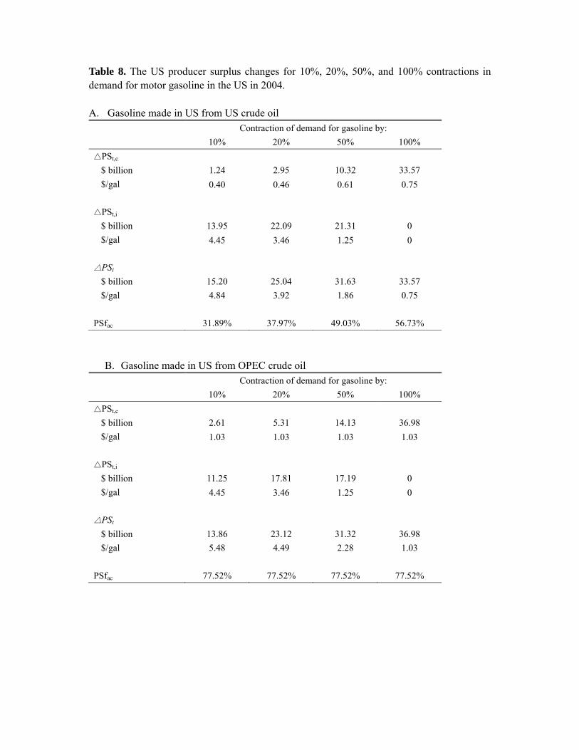
Table 8. The US producer surplus changes for 10%, 20%, 50%, and 100% contractions in demand for motor gasoline in the US in 2004. A. Gasoline made in US from US crude oil

Contraction of demand for gasoline by:

10% 20% 50% 100%

△PSt,c

$ billion

$/gal

1.24

2.95

10.32

33.57

0.40 0.46 0.61 0.75

△PSt,i

$ billion

$/gal

13.95

22.09

21.31

0

4.45 3.46 1.25 0

△PSt

$ billion

$/gal

15.20

4.84

25.04

3.92

31.63

1.86

33.57

0.75

PSfac 31.89% 37.97% 49.03% 56.73%

B. Gasoline made in US from OPEC crude oil Contraction of demand for gasoline by:

10% 20% 50% 100%

△PSt,c

$ billion

$/gal

2.61

5.31

14.13

36.98

1.03 1.03 1.03 1.03

△PSt,i

$ billion

$/gal

11.25

17.81

17.19

0

4.45 3.46 1.25 0

△PSt

$ billion

$/gal

13.86

5.48

23.12

4.49

31.32

2.28

36.98

1.03

PSfac 77.52% 77.52% 77.52% 77.52%

C. Gasoline made in US from ROW crude oil

Contraction of demand for gasoline by:

10% 20% 50% 100%

△PSt,c

$ billion

$/gal

3.37

6.85

18.24

47.74

1.02 1.02 1.02 1.02

△PSt,i

$ billion

$/gal

14.67

23.23

22.41

0

4.45 3.46 1.25 0

△PSt

$ billion

$/gal

18.04

5.47

30.08

4.48

40.65

2.27

47.74

1.02

PSfac 76.73% 76.73% 76.72% 76.72%

D. Gasoline made in US (all: sum of A, B, and C) Contraction of demand for gasoline by:

10% 20% 50% 100%

△PSt,c

$ billion

$/gal

7.22

15.11

42.69

118.29

0.80 0.83 0.88 0.93

△PSt,I

$ billion

$/gal

39.88

63.13

60.91

0

4.45 3.46 1.25 0

△PSt

$ billion

$/gal

47.10

5.25

78.24

4.29

103.60

2.13

118.29

0.93

PSfac 61.26% 63.39% 67.26% 69.95%

As shown in Table 8, the producer surplus associated with all gasoline use in the US in 2004 (i.e., the producers surplus for a 100% reduction in gasoline use) was $33.57 billion in the US, $36.98 billion for OPEC and $47.74 billion for the ROW. The total wealth transfer from US consumers to foreign producers thus was $84.72 billion (OPEC plus ROW). The wealth transfer from US consumers to foreign producers is much larger than the transfer from

consumers to domestic producers because foreign producers have much lower average costs and hence earn much higher producer surplus.

6.2 Analysis of producer surplus as a function of change in total gasoline supply in the US over the period 2005-2030

With the derived future gasoline cost curve (section 5.5.2), which includes both oil recovery and refining for the period 2005 to 2030, we can calculate the producer surplus as the area below the gasoline price ($2.75/gal, the average gasoline price from 2005 to 2030) and above the marginal cost curve integrated from 0 to 132.80 million gallons per day. The resulting producer surplus fraction with respect to price-times-quantity payments is 40.5%, much lower than the 2004 level. This is to be expected, because we simply have shifted the cost curve up without changing its shape, which means that the cost portion of price-times-quantity payments – the area under the long-run marginal cost curve – will be larger in the future than it was in 2004. To estimate the producer surplus for OPEC and ROW beyond 2004, we simply repeat what we did for year 2004 in Section 5.4 using the World Bank data for each year t from 1992 to 2003, assuming the same functional form as in Equation 7. Then we obtain time-dependent coefficients c(t) and d(t) for OPEC and ROW respectively. We regress each coefficient on time to estimate the trend, based on which we estimate future marginal cost for OPEC and ROW. Since the coefficients d(t) for OPEC or ROW from 1992 to 2003 show little variation, we just take the average. Our results for the marginal costs for OPEC and ROW are as follows:

)*10*6.1exp(*)ln(*396.0 ,4

, tOPECtOPEC QtMC (29)

)*10*76.1exp(*)ln(*28.1 ,5

, tROWtROW QtMC . (30)

In this analysis, we choose the year 2025 to estimate producer surplus for OPEC and ROW with world crude oil price, oil import share, US domestic oil supply, total gasoline supply in the US, and US gasoline price in 2025 from EIA AEO 2014 reference case. For future oil production for OPEC and ROW, OPEC and DOE/EIA have different projections as shown in Table 9. To simplify our analysis, we use the mean value of these estimates. Table 10 presents our estimates of total producer surplus change for gasoline made in the US from OPEC and ROW crude oil for 10%, 20%, 50%, and 100% of contractions of demand for motor gasoline in the US

Table 9. Projections for 2025 oil supply from OPEC and DOE/EIA (million barrels per day)

OPEC 54.3

(incl. NGLs)

41

(incl. NGLs, about 79% is crude oil)

57

(incl. NGLs)

46

(high price)

61

(reference)

71

(low price)

Non-OPEC 58.9 60.1 56.4

Source Barkindo, 2006 OPEC, 2012 Qabazard, 2006 EIA 2003 EIA 2003 EIA 2003

Note: the percentage 79% (OPEC, 2012) was used to estimate crude oil production from the other two sources (Barkindo, 2006, Qabazard, 2006).

Table 10. The foreign producer surplus changes for 10%, 20%, 50%, and 100% contractions in demand for motor gasoline in the US in 2025

A. Gasoline made in US from OPEC crude oil Contraction of demand for gasoline by:

10% 20% 50% 100%

△PSt ($billion) $20 $34.90 $48.82 $53.26

PSfac 77.33% 77.33% 77.33% 77.33%

B. Gasoline made in US from ROW crude oil Contraction of demand for gasoline by:

10% 20% 50% 100%

△PSt ($billion) $30.23 $52.74 $73.71 $80.23

PSfac 77.01% 77.01% 77.01% 77.01%

7. Discussion

Our estimates of producer surplus confirm that the average cost of gasoline in the US is much less than the price paid by consumers. This result has important implications for estimates of wealth transfers from oil consumers to oil producers as part of an analysis of the total costs and benefits to the US of policies related to oil use and oil imports, and for analyses involving the social cost of gasoline (e.g., comparisons of the social cost of gasoline vehicles versus the social cost of hydrogen vehicles). 7.1 Producer surplus in estimates of wealth transfers as a result of policies affecting US oil use

As a result of much lower average oil cost of OPEC and ROW than that of the US, the producer surplus fraction PSfac was quite high (more than 75%) for gasoline made in the US from imported oil in 2004 and it did not change much with gasoline use contraction. Our estimate for 2025 shows that the producer surplus associated with the US gasoline use is larger for both OPEC and ROW than that in 2004 primarily due to high oil price projected in 2025. Policies that reduce the US oil use would greatly reduce the wealth transfer from the US to the foreigners. 7.2 Producer surplus in comparisons of the social cost of transportation fuels

To illustrate the importance of treating producer surplus properly in cost-benefit analysis of transportation fuels, we summarize and update the results of a previous analysis (Sun et al., 2010) of the social lifetime cost of hydrogen fuel cell vehicles compared with conventional

gasoline vehicles. The social lifetime cost includes the vehicle retail cost, fuel cost, operating and maintenance costs, externality costs of oil use, noise damage costs, air pollution damage costs, climate change damage costs, and adjustments for non-cost social transfers including taxes and fees and producer surplus associated with fuels and vehicles. We estimate the social lifetime cost from two perspectives: (1) a global perspective, which counts all climate change damages everywhere in the world but ignores all producer-surplus wealth changes as non-cost transfers between global producers and consumers, and (2) a US perspective, which counts climate change damages only in the US but does count as a cost to US consumers wealth transfers of producer surplus to foreign countries. Table 11 shows the results of the analysis. In addition to showing the internally consistent US and global perspectives, Table 11 also shows two common, incorrect perspectives: a hybrid estimate of the SLC, in which climate change damages from the global perspective are added to producer surplus losses from the US perspective, and a perspective that counts all producer surplus as a cost; i.e., uses pre-tax price times quantity as the fuel cost. The results of Table 11 show that analyses (e.g., Goedecke et al., 2007, Ogden et al., 2004) that incorrectly use price-times-quantity payments and hence incorrectly include producer surplus in an estimate of the social cost of gasoline will overestimate the present value lifetime social cost of gasoline vehicles by $2,280 to $9860. According to our results in Table 11, the social lifetime cost of gasoline vehicles is $70,534 from a US perspective and $67,454 from a global perspective, both of which are slightly higher than the social lifetime cost of hydrogen fuel cell vehicles, which is $65,377.

Table 11. Social lifetime cost of hydrogen fuel cell versus gasoline vehicles in 2025 (Present value of cost streams over life of vehicle; 2005 USD)

Gasoline Hydrogen(US) Correct:

US losses Correct: global losses

Incorrect: hybrid

US/global

Incorrect: all

producer surplus is

a cost Fuel cost excluding taxes $4,906 $4,906 $4,906 $4,906 $6,102 Fuel taxes $1,763 $1,763 $1,763 $1,763 $1,904 Fuel producer surplus $4,704 0 $4,704 $7,087 $132 Climate change damages $333 $2,613 $2,613 $2,613 $213 Other external costs $13,090 $12,434 $13,090 $12,434 $4,603 All other costs $45,739 $45,739 $45,739 $48,507 $52,423 Total $70,534 $67,454 $72,815 $77,310 $65,377 Notes: All values except producer surplus are from Ref. (Sun et al., 2010), using high estimates of external costs. Producer surplus estimates here are equal to fuel cost without producer surplus adjustment multiplied by the ratio of producer surplus without producer surplus adjustment to fuel cost, where this ratio is from the analysis here (0.405 for the US producers and 0.77 for foreign producers). The treatment of producer surplus for hydrogen fuel is discussed in Appendix B.

8. Conclusion

Estimating the producer surplus is an important part of social cost-benefit analyses of changes in petroleum use. This paper estimates the producer surplus associated with changes in gasoline fuel use in the United States, and then applies the estimates of producer surplus to two kinds of social cost-benefit analyses related to petroleum use: (1) estimating the wealth transfer from consumers to producers as a result of policies that affect oil use and oil importing in the US, and (2) comparing the actual average cost of gasoline (where the average cost is the observed price minus the estimated fraction of price that is producer surplus) with the average cost of environmentally superior alternatives to gasoline, such as hydrogen. According to our results, both kinds of producer surplus estimates depend on the size of the reduction in oil use and the year and region for which oil cost curves are estimated. We estimate that if demand for gasoline in the US in 2004 had contracted by 10% (50%), then the change in producer surplus in the US refinery and US oil industry would have been $15.2 ($31.63) billion, or $4.84 ($1.86) per gallon of gasoline, and the producer surplus fraction of revenues would

have been 31.89% (49.03%). The change in producer surplus for gasoline made from imported oil would have been greater – $5.48/gallon for a 10% contraction and $2.28/gal for a 50% contraction – because foreign producers have much lower average production cost. In fact, a 50% reduction in gasoline use in the US in 2004 would have saved the US $94 billion in producer surplus payments to foreign oil producers. Applying our estimates to the comparison of the social lifetime cost of hydrogen vehicles versus gasoline vehicles, we find that inconsistently counting producer surplus from a US national perspective while counting climate change damages from a global perspective can overstate the present value lifetime costs of gasoline vehicles by $2,200 to $9,800 per vehicle. Because there is a large cost difference between low-cost and high-cost oil producers, and because OPEC manipulates output to control prices, many oil producers, but especially those in OPEC, enjoy very large economic rent and economic profit, which together compose producer surplus. In 2004, US drivers paid $278 billion for gasoline, of which $92 billion was taxes, $58 billion was actual economic cost, and $128 billion – the largest portion – was producer surplus. From a global perspective, this producer surplus was just a transfer from consumers to producers. However, from the perspective of the US, the producer surplus paid to foreign oil producers -- $84.7 billion in 2004 -- was a real cost. In future years, the producer surplus would be even larger, for example, $122.5 billion in 2025 based on our analysis. However, in cost-benefit analyses, one may treat producer surplus as a cost only if one takes a limited domestic perspective and ignores the welfare of foreign producers. And if one does take a domestic perspective regarding producer surplus, one must take a domestic perspective regarding all components of the social cost, including climate change damages. A reduction in gasoline use has greater producer surplus benefits but lower climate change damage benefits in a domestic as compared to a global perspective. For example, EIA AEO 2013 reference case projects that motor gasoline consumption in the US in 2025 is 13.86 quadrillion Btu. A 50% reduction in gasoline use in the US in 2025 would save the US $168 billion in producer surplus lost to foreign countries, assuming 50% is from foreign oil and US $2.6 billion in climate change damages for LDV12 only in the US, every year. However, from a global perspective, the 50% reduction in gasoline use in the US would save nothing in terms of producer surplus (which from a global perspective is just a transfer from consumers to producers) but would save US $20 billion per year in climate change damages to the world. An inconsistent treatment of producer surplus and climate change damages thus can result in an error of hundreds of billions of dollars in cost–benefit analyses. The producer surplus estimates developed in this study can be used to avoid these errors.

12 The US LDV vehicle miles traveled in 2025 is 3,089 billion under EIA AEO2013 reference case.

References

Aguilera, Roberto F. (2014). Production costs of global conventional and unconventional petroleum. Energy Policy, 64, 134-140.

American Petroleum Institute [API]. (2004). Joint Association Survey on Drilling costs, Washington, D.C.

American Petroleum Institute [API]. (1989). Survey on oil and gas expenditures for exploration, development, and production, Washington, D.C.

Augustine, Chad, Jefferson W. Tester and Brian Anderson. (2006). A Comparison of Geothermal with Oil and Gas Well Drilling Costs, Proceedings, Thirty-First Workshop on Geothermal Reservoir Engineering, Stanford University, Stanford, California, January 30-February 1, 2006, SGP-TR-179.

Barkindo, Mohanned. (2006). Oil Outlook to 2025, 10th International Energy Forum, Doha, 22nd-24th April 2006. URL: http://www.opec.org/opec_web/static_files_project/media/downloads/publications/IEFBarkindo.pdf

Bentham, Jeremy. (2014). The scenario approach to possible futures for oil and natural gas. Energy Policy, 64, 87-92.

Biedermann, Gerhard. (1961). The Cost Function for Crude Oil Production. The Manchester School, 29 (3), 49-265.

Boyes, William, and Michael Melvin. (2008). Microeconomics, Seventh Edition, Chapter 10 Perfect Competition, 2. The Long Run, 2.b. Normal Profit in the Long Run.

Chakravorty, Ujjayant, James Roumasset and Kinping Tse. (1997). Endogenous Substitution among Energy Resources and Global Warming. Journal of Political Economy, 105 (6), 1201-1234.

Cleveland, Cutler J. (1991). Physical and economic aspects of resource quality – The cost of oil supply in the lower 48 United States, 1936-1988. Resources and Energy, 13, 163-188.

Delucchi, Mark A. (2004). Motor-vehicle Goods and Services Priced in the Private Sector, Report #5 in the series: The Annualized Social Cost of Motor-Vehicle Use in the United States, based on 1990-1991 Data, UCD-ITS-RR-96-3 (5), October 2004.

Delucchi, Mark A. (2005). AVCEM: Advanced-Vehicle Cost and Energy-use Model – AVCEM documentation part 1: Overview of AVCEM, UCD-ITS-RR-05-17 (1).

Energy Information Administration [EIA]. (2003). Annual Energy Outlook 2003 with Projections to 2025. URL: http://books.google.com/books?id=yNTRXg_1PrIC&pg=PA52&lpg=PA52&dq=OPEC+production+2025&source=bl&ots=_D8uYG61hx&sig=4Ko9yGctH93-5uIUwFrlLjuTK6Q&hl=en&sa=X&ei=ibK4Uo21KdLpoASzGg&ved=0CEwQ6AEwBA#v=onepage&q=OPEC%20production%202025&f=false

Energy Information Administration [EIA]. (2008a). Financial Reporting System – Form EIA-28 2008 Petroleum Operations.

Energy Information Administration [EIA]. (2008b). US Natural Gas Gross Withdrawal (MMcf). URL: http://tonto.eia.doe.gov/dnav/ng/hist_xls/N9010US2a.xls. Accessed September 29, 2009.

Energy Information Administration [EIA]. (2009a). Annual Energy Outlook 2009

Energy Information Administration [EIA]. (2009b). Annual Energy Review Report No. DOE/EIA-0384. URL: www.eia.gov/emeu/aer/contents.html

Energy Information Administration [EIA]. (2010). International Energy Module of the National Energy Modeling System: Model Documentation 2010, DOE/EIA-M071.

Energy Information Administration [EIA]. (2010a). Documentation of the Oil and Gas Supply Module (OGSM), DOE/EIA-M063.

Energy Information Administration [EIA]. (2010b). Petroleum Market Model of the National Energy Modeling System: Model Documentation 2010, Part 1 – Report and Appendix A, DOE/EIA-M059. Part 1.

Energy Information Administration [EIA]. (2011). Monthly Energy Review, March 2011, Tables 3.1 and 3.3b and Annual Energy Review, Table 5.3.

Energy Information Administration [EIA]. (2014). Annual Energy Outlook 2014 early release. URL: http://www.eia.gov/forecasts/aeo/er/early_prices.cfm. Accessed December 26, 2013.

Frank, Robert H., and Ben S. Bernanke. (2003). Principles of Microeconomics, Second Edition, Chapter 8, The Quest for Profit and the Invisible Hand.

Goedecke, Martin, Supaporn Therdthianwong, and Shabbir H. Gheewala. (2007). Life cycle cost analysis of alternative vehicles and fuels in Thailand. Energy Policy, 35, 3236-3246.

Greene, D.L., and N. I. Tishchishyna. (2009). Costs of Oil Dependence: A 2000 Update, Oak Ridge National Laboratory, ORNL/TM-2000/152, Oak Ridge, TN, 2000, and data updates.

Hotelling, Harold. (1931). The Economics of Exhaustible Resources. Journal of Political Economy, 3 (2), 137-175.

International Energy Agency. (2009). World Energy Outlook 2009. URL: http://www.iea.org/speech/2009/birol_moscow.pdf. Accessed June 25, 2010.

Jakobsson, Kristofer, Bengt Söderbergh, Simon Snowden, Kjell Aleklett. (2014). Bottom-up modeling of oil production: A review of approaches. Energy Policy, 64, 113-123.

Kaiser, Mark J. (2007). A Survey of Drilling Cost and Complexity Estimation Models. International Journal of Petroleum Science and Technology 1 (1), 1-22.

Khatib, Hisham. (2014). Oil and national gas prospects: Middle East and North Africa. Energy Policy, 64, 71-77.

Leiby, Paul N. (1993). A Methodology for Assessing the Market Benefits of Alternative Motor Fuels – The Alternative Fuels Trade Model, ORNL-6771.

Lemus, Ricardo Guerrero, and José Manuek Martínez Duart. (2010). Updated hydrogen production costs and parities for conventional and renewable technologies. International Journal of Hydrogen Energy, 35, 3929-3936.

Lin, C.-Y. Cynthia, and Gernot Wagner (2007), Steady-state growth in a Hotelling model of resource extraction. Journal of Environmental Economics and Management, 54, 68-83.

Nicholson, Walter. (2004). Microeconomic Theory – Basic Principles and Extensions, 9th Edition, Chapters 8 and 9.

Ogden, Joan M., Robert H. Williams, and Eric D. Larson. (2004). Societal lifecycle costs of cars with alternative fuels/engines. Energy Policy, 32, 7-27.

OPEC. (2012). World Oil Outlook 2012. URL: http://www.opec.org/opec_web/static_files_project/media/downloads/publications/WOO2012.pdf

Pindyck, Robert S., and Daniel L. Rubinfeld. (2004). Microeconomics, Sixth Edition, Part 2. Producers, Consumers, and Competitive Markets.

Qabazard, Hasan M. (2006). Global Oil Outlook up to 2025, Annual General Assembly of the InternationAL Chamber of Commerce – Austria, Vienna, June 22, 2006. URL: http://www.opec.org/opec_web/static_files_project/media/downloads/press_room/IntChamComm.pdf

Sun, Yongling, Joan Ogden, and Mark Delucchi. (2010). Societal lifetime cost of hydrogen fuel cell vehicles. International Journal of Hydrogen Energy, 35, 11932-11946.

US Census Bureau, Economic Census, Mining: Industry Series: Detailed Statistics by Industry for the United States: 1987-2007.

Yang, Christopher and Joan M. Ogden. (2007). Determining the lowest-cost hydrogen delivery mode. International Journal of Hydrogen Energy, 32, 268-286.

Appendix A.

Table A1. Glossary of terms relevant to the discussion of producer surplus

Producer surplus: revenue received by producers from selling goods at the market price over and above the long-run average cost. It comprises economic profit and economic rent (Figure 2).

Economic profit: total revenue minus economic rent and economic cost. Economic profit is zero in long-run equilibrium in perfect competition. Hence, economic profit is the portion of producer surplus that arises in non-competitive markets, such as oligopolies.

Economic rent: extra payment for an input that firm is willing to pay over the minimum amount necessary to retain it in its current use (the opportunity cost of the input). Economic rent is the portion of producer surplus that is not due to non-competitive markets; in competitive markets in the long-run equilibrium, producer surplus = economic rent. Economic rent arises when some firms have exclusive access to low-cost factors of production, such as large, easy-to-exploit mineral reserves, technology protected by patents, or captive cheap labor.

Normal profit (implicit costs): The portion of revenue identified with implicit cost. Whereas in the long run in perfect competition economic profit is zero, normal profit is nonzero (Boyes and Melvin, 2008). Normal profit, based on a “normal” rate of return to investment, is not a component of producer surplus (Figure A1).

Explicit cost (also accounting cost): accounted cost that firms have to pay in the form of money; distinguished from “implicit” costs.

Economic cost (also resource cost, or opportunity cost, or long-run marginal cost): payment required to employ inputs for production; equal to implicit plus explicit costs (Figure 2). The long-run marginal cost curve represents economic cost.

Long-run average cost: the area under the long-run marginal cost curve for ∆Q, divided by ∆Q.

Note: For a detailed discussion, see Nicholson (2004) and Pindyck and Rubinfeld (2004).

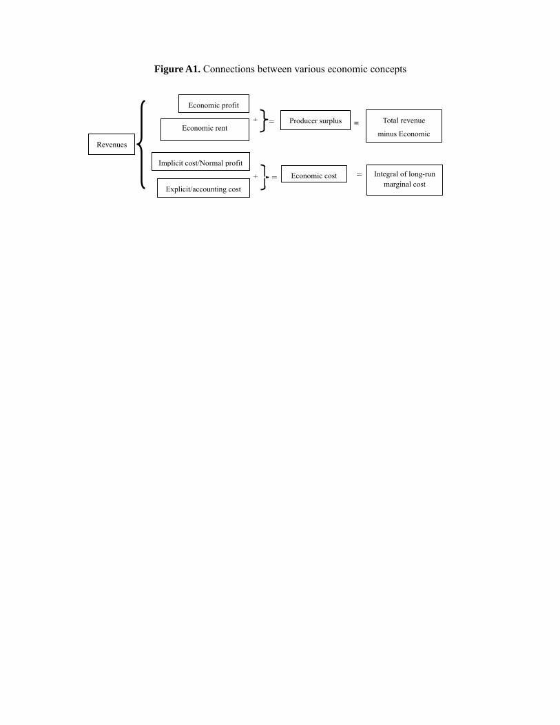
Figure A1. Connections between various economic concepts

+

+

Economic profit

Integral of long-run marginal cost

Economic cost

Economic rent =

Explicit/accounting cost

= =

= Total revenue

minus Economic

Implicit cost/Normal profit

Revenues

Producer surplus

Appendix B.

Estimates of the cost of hydrogen fuel are not derived from market prices (which for future hydrogen fuels do not exist), but rather are built from detailed engineering cost studies and hence are direct estimates of average economic cost. This means that in a comparison of the social cost of hydrogen vehicles with the social cost of gasoline vehicles, one does not need to subtract the producer surplus from the estimates of hydrogen cost. However, in a comparison of the private cost – the cost the consumer pays – one must estimate the price the consumer faces rather than the average cost. Because price projections are not available for hydrogen, one must estimate the price of hydrogen by adding the producer surplus to the aforementioned engineering estimates of the average cost of hydrogen. Table A1 summarizes the conceptual estimation of the social cost and the private cost of fuel for gasoline and hydrogen. Table B1. Conceptual framework for the estimation of the social cost and the private cost of gasoline and hydrogen.

Gasoline Hydrogen

Private cost Projections of gasoline price, e.g. from the EIA (2009a)

Estimated average cost plus estimated producer surplus

Social cost Projected gasoline price minus estimated producer surplus

Engineering estimates of average economic cost, e.g. Lemus and Duart

(2010)

We have not analyzed the potential producer surplus on sales of hydrogen fuel. However, we believe the regional-market marginal cost curve for producing hydrogen is likely to be relatively flat, and that hence the price is likely to be close to the average cost. For example, imagine that we have a national program to produce hydrogen from wind or photovoltaic electrolysis of water. Suppose that half of the total hydrogen supply can be produced in windy or sunny areas at a relatively low cost, while the other half must be produced in less well-endowed areas at a relatively high cost. If there was a single national market, in which all producing regions were connected to all consuming regions by inexpensive transportation modes, then there would be a single national price of hydrogen equal to the marginal cost of the high-cost producers plus transportation costs. In this case, the low-cost producers would enjoy considerable producer surplus. This would be analogous to the situation with oil today, in which oil can be transported anywhere in the world for a small fraction of the cost of marginal oil production. However, the transport of hydrogen is expensive, and varies considerably with distance (Yang and Ogden, 2007). Regions with high-cost primary energy sources (less solar or wind energy) will pay either for high-cost energy plus low-cost transport, or low-cost energy

plus high-cost long-distance transport, whereas regions with low-cost primary energy sources will pay for low-cost energy plus low-cost, local transport. Thus, in a realistic hydrogen scenario there will be significant regional price heterogeneity, and in any one region, average cost will not be much less than marginal cost price. This is similar to the case for electricity today, where power costs vary considerably by region, and very long distance transport of power is rare.