the productivity growth slowdown by industry - … · the productivity growth slowdown by industry...

MARTIN NEIL BAILY Brookings Institution

The Productivity Growth Slowdown by Industry

LABOR productivity growth for the private economy as a whole seems to have stopped altogether. In the first half of 1982 the U.S. Bureau of Labor Statistics index of private sector labor productivity was below its 1977 level. Productivity has stagnated for five years. Weak aggregate demand has been an ingredient in this stagnation, but cannot account for much of it. Even in the 1930s there was only a four-year stagnation of productivity accompanying a much more severe fall in demand. By 1934, productivity was above its 1929 level.

This paper is part of a continuing research project to understand and explain the slowdown. In earlier work I looked at the aggregate picture. I In this paper I report on the behavior of productivity at the industry level-the major industry groups and the two-digit manufacturing industries. In future work I will analyze the behavior of individual firms and establishments.

The paper focuses on the following questions. (1) Does the incidence of the productivity slowdown by industry suggest that capital services have declined relative to the capital stock? (2) Does it suggest that the rate of technical change has slowed? (3) Have responses to the increased cost of energy been a major cause of the slowdown? (4) Have changes

The research upon which this paper is based was funded in part by a grant from the Office of the Assistant Secretary for Policy Evaluation and Research of the U.S. Department of Labor (contract J-9-M-0-0 18 1). I would like to thank Karen Hanovice, Lisa James, Judith D. Kleinman, and Suzanne Wehrs for assistance. I have received many helpful comments from members of the Brookings Panel.

1. Martin Neil Baily, "Productivity and the Services of Capital and Labor," BPEA, 1:1981, pp. 1-50.

423

424 Brookings Papers on Economic Activity, 2:1982

in the distribution of output or employment among industries contributed to the slowdown in aggregate labor productivity?

The Analytical Framework

For expositional convenience, the analytical framework is developed using Cobb-Douglas production functions. All numerical estimates derived subsequently allow factor shares to change over time and so assume only that the production function is well behaved and exhibits constant returns to scale.2

Output in industry i is Qi and is produced by capital services, KSi, and labor services, Li, with the following specification:

( 1 ) Qi = Aieyi' (KS) I - oi Lioi,

where Ai is a constant, -y, is the rate of technical change, and (xi is the labor coefficient. Using lowercase letters to denote logarithmic rates of change, equation 1 implies

(2) qi = y1 + (1 - oti)ksi + otili.

There is no direct observation of capital services, but there is data on the capital stock, Ki. The ratio of capital services to the capital stock is called KRi; its rate of change is expressed as

(3) kri = ksi - ki.

CAPITAL AND LABOR PRODUCTIVITY

I next define a concept called capital and labor productivity, KLP, with a rate of change given by

(4) klpi = qi- (1 - o)ki - oili.

The KLP concept is clearly similar to that of total factor productivity, which is widely used in the literature. I use the term KLP because the growth rate of KLP depends not only upon the rate of technical change,

2. This issue is clarified in Barbara M. Fraumeni and Dale W. Jorgenson, "Capital Formation and U. S. Productivity Growth, 1948-1976, " in Ali Dogramaci, ed., Productivity Analysis: A Range of Perspectives (Martinus Nijhoff Publishing, 1981), pp. 49-70.

-_= >t** .. s I -s --..t I --

but also upon movements in KR, the ratio of capital services to the capital stock.

Substituting equations 3 and 4 into 2 gives

(5) klpi = yi + (1 - oi)kri.

As shown below, the rate of growth of KLP has decreased in most of the industries in the private business sector of the U.S. economy since 1973. The symbol /\ denotes the change in the rate of growth of a variable between two periods, so that

(6) zklpi = A-yi + (1 - cx) Akri.

The variation in KLP growth is then the sum of the variations in the rate of technical change and in the rate of change of the capital services ratio weighted by capital intensity.

DIFFERENCES IN CAPITAL INTENSITY

If there were no changes in any of the -yi and if A\kri was the same in all industries, the magnitudes of the KLP declines by industry would de- pend upon the oxi. In other words, if there has been a general decline in the ratio of capital services to the capital stock since 1973, the KLP slowdown will have been greatest in the capital-intensive industries.

DIFFERENCES IN THE BEHAVIOR OF

THE CAPITAL SERVICES RATIO

It is unlikely that changes in kri were in fact the same in all industries. One reason for differences might be differences in energy intensity. If much of the old capital stock has had to be replaced by more energy- efficient capital, and if the measurement of the capital stock does not take this obsolescence into account, the measured capital services ratio will have fallen. This ratio will also have fallen if recent investment, and hence the measured capital stock, has been disproportionately devoted to environmental protection rather than production, or if an industry has had to completely retool for a new product line. One can look across industries to see if energy intensity or other information indicates possible causes of declines in the capital services ratio.


The term A\kri in equation 6 reflects any breaks in the trend growth rate of the capital services ratio, positive or negative. Instead of asking why productivity growth slowed down after 1973 one could just as well ask why growth was rapid before 1973. It could be that in some industries favorable factors were allowing the capital services ratio to rise before 1973 and that these favorable movements slowed or ceased after that year.

DECLINES IN THE RATE OF TECHNOLOGICAL CHANGE

Technological change reflects improvements in knowledge that are transmitted in some way to the production process-by organizational changes or by embodiment in the capital. Technological possibilities differ in different industries. Some are mature and have slow rates of growth and others experience rapid rates of technical change. The flow of new technology is taking place primarily in the industries with rapid growth. The different stages of maturity are illustrated below.

The slope of the S-curve in the diagram indicates the rate of productivity growth at different stages in an industry's life. An industry with a newly emerging technology is near point A. A comparison of time periods will show its productivity growth rate beginning to increase. A mature industry, on the other hand, is one that has already reached a point like C at the beginning of the sample period. A comparison of subperiods shows a growth slowdown, but it will be only slight. Industries that are intermediate between these cases show rapidly accelerating productivity growth as they move from A to B, and then stable but high rates of productivity growth along the steep portion of the curve around B. They show large slowdowns in growth as they move from B to C.

If the KLP growth slowdown has come about because there have been relatively few if any newly emerging technologies in recent years, most of the industries one observes will be beyond the inflection point B. Some of these industries were already mature in the 1950s and 1960s, and will show little slowdown. They were already at point C at the beginning of the sample period. Industries that were on the steep part of the curve in the 1950s and 1960s should show large slowdowns as they became mature industries. If the population of industries is dominated by firms in this latter part of their productivity cycle, it would indicate that industries that were previously growing rapidly are becoming mature

Martin Neil Baily 427

Level of productivity

~~~~productivity growth

Large slowdowns productivity growth

Accelerating productivity growth

|A

Age of industry

and that there are few newly emerging technologies. This would explain the observed KLP slowdown.

Another clue about the source of the slowdown comes from the fact that a negative rate of technical change seems implausible. If there have been negative rates of change of KLP in some industries or in the aggregate, then it is unlikely that a decline in the flow of new technology is the sole reason for the slowdown.

LABOR PRODUCTIVITY

Average labor productivity, ALP, is the most familiar measure of productivity. It is the slowdown in labor productivity growth that calls attention to the productivity puzzle. Equation 2 implies that


(7) alpi = -yi + (1 - oi)(ksi- 1).

ALP grows at a rate depending upon the rate of technical change and the growth rate of the ratio of capital services to labor input. Substituting 3 and 5 into 7, the change in ALP growth can be expressed as

(8) lAalpi = LAyi + (1 - ot)z\kri + (1 - ot) A (ki - l1) = zklpi + (1 - ot) A (ki - li).

The slowdown in labor productivity growth is the weighted sum of the variations in the rate of technical change, the rate of change of the capital services ratio, and the rate of growth of the ratio of the capital stock to labor input. The difference between the ALP slowdown and the KLP slowdown is just the last of these three terms. If the ratio of capital stock to labor grew more slowly after 1973, the slowdown in labor productivity growth will be greater than the slowdown in KLP growth. Hence trends in capital formation may help to explain the labor productivity slowdown in particular industries.3

THE EFFECT OF DEMAND FLUCTUATIONS

When business firms vary their production as a result of fluctuations in product demand, there are corresponding variations in the intensity with which the factors of capital and labor are used. Labor services, denoted by L in the preceding discussion, refer to hours worked as measured by the Bureau of Labor Statistics. During a period of slack demand, actual labor services, denoted by LS, fall before measured labor hours do because of labor hoarding and variations in work intensity. During a peak period actual labor services will be above L, as extra effort is given by the work force. When output is equal to potential output (denoted by Q*), measured labor input (denoted by L*) is assumed to be equal to actual labor services, or L* = LS*.

3. With more information, it would be possible to make more of the gaps between the ALP and the KLP slowdowns, because for any particular industry investment behavior is influenced by other changes. For example, an increase in the rate of technical change might stimulate demand for the industry's product by its effect on prices. This would stimulate capital formation. But capital expenditures could also be stimulated by some "adverse" event-such as a new regulation of the Occupational Safety and Health Administration (OSHA)-that also leads to a decline in productivity growth. In practice the case that is relevant is difficult to determine.


Because capital is to some extent putty-clay in nature, it follows that capital services also fluctuate in the short run with output fluctuations. The preceding model has already distinguished between the flow of capital services and the capital stock, so that in principle weak demand could simply be one reason why the ratio of capital services to capital stock might have declined after 1973. But it makes an important difference whether the decline in output-producing capital services is the result of low industry demand or more permanent structural problems. The level of capital services achieved when output is at potential is denoted by KS*. It is the movements of KS* relative to the capital stock, K, that are of primary interest in understanding the slowdown.

In order to isolate the effects on productivity trends, I now modify equation 1 to allow explicitly for demand fluctuations. Actual output, Qi, and potential output, QO, are

(9) Qi = Ai eY i(KSi) I - Oi (LSi)o

Qi* = AieYi'(KSP)1 - i (L*)o.

Actual and potential KLP are defined by

(10) ln KLPi = ln Qi - oi ln Li - (1 - oxi) ln Ki

In KLP:* = In Qi* - oti In LP* - (I - oxi) In Ki.

From 9 and 10 it follows that

(I11) In KLPi* = In KLPi - (I - oti)In KS* oti In LS. KS, Li

Demand-adjusted or potential productivity differs from actual KLP because of deviations of capital services from their potential level and because of deviations of actual labor services from measured labor input. Note that these capital and labor terms are not symmetric. A persistent recession, such as the situation that has occurred in the past few years, will leave KSi below KSP. But after several years of recession, one would expect Li and LSi to become equal as work practices return to normal and hoarded labor is eliminated.

In the two-digit manufacturing industries there is a straightforward way of estimating KLP*. The Federal Reserve Board surveys manufac-


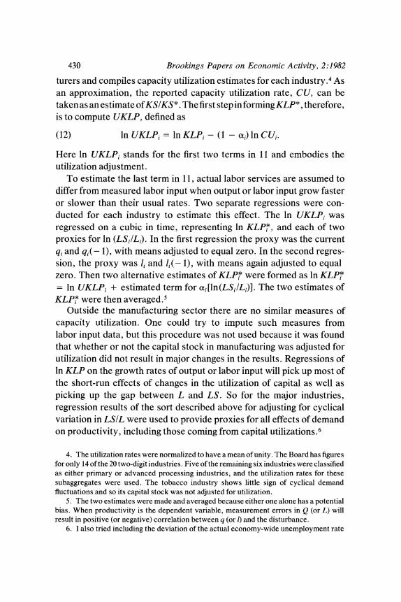
turers and compiles capacity utilization estimates for each industry.4 As an approximation, the reported capacity utilization rate, CU, can be taken as an estimate of KSIKS*. The first step in forming KLP*, therefore, is to compute UKLP, defined as

(12) In UKLPi = ln KLPi - (1 - oxi) ln CUi.

Here ln UKLPi stands for the first two terms in 11 and embodies the utilization adjustment.

To estimate the last term in 11, actual labor services are assumed to differ from measured labor input when output or labor input grow faster or slower than their usual rates. Two separate regressions were con- ducted for each industry to estimate this effect. The ln UKLPi was regressed on a cubic in time, representing ln KLP*, and each of two proxies for ln (LSilLi). In the first regression the proxy was the current qi and qi(- 1), with means adjusted to equal zero. In the second regression, the proxy was 1i and lQ(- 1), with means again adjusted to equal zero. Then two alternative estimates of KLP* were formed as ln KLP*

ln UKLPi + estimated term for aiJln(LSi1Li)]. The two estimates of KLP* were then averaged.S

Outside the manufacturing sector there are no similar measures of capacity utilization. One could try to impute such measures from labor input data, but this procedure was not used because it was found that whether or not the capital stock in manufacturing was adjusted for utilization did not result in major changes in the results. Regressions of ln KLP on the growth rates of output or labor input will pick up most of the short-run effects of changes in the utilization of capital as well as picking up the gap between L and LS. So for the major industries, regression results of the sort described above for adjusting for cyclical variation in LSIL were used to provide proxies for all effects of demand on productivity, including those coming from capital utilizations.6

4. The utilization rates were normalized to have a mean of unity. The Board has figures for only 14 of the 20 two-digit industries. Five of the remaining six industries were classified as either primary or advanced processing industries, and the utilization rates for these subaggregates were used. The tobacco industry shows little sign of cyclical demand fluctuations and so its capital stock was not adjusted for utilization.

5. The two estimates were made and averaged because either one alone has a potential bias. When productivity is the dependent variable, measurement errors in Q (or L) will result in positive (or negative) correlation between q (or 1) and the disturbance.

6. I also tried including the deviation of the actual economy-wide unemployment rate


These fairly elaborate adjustments for demand were made because demand fluctuations have been large and their effects could have been important. However, the incidence of the slowdown across industries turns out to be quite robust to the form of the demand adjustment that is made or even to whether or not an adjustment is made. The inferences discussed in the paper were not created by the demand adjustment.

The Slowdown in the Major Industries

The productivity slowdown can be described for the different industries by three statistics derived from the preceding analysis: the slowdown in labor productivity growth, the KLP slowdown, and the KLP* slowdown-the KLP slowdown adjusted for demand fluctuations. Table 1 describes the productivity growth slowdown in the major industry groups of the private business sector using these statistics.7 The table indicates the following general results.

The slowdown is pervasive. Only one industry shows an acceleration of labor productivity growth and only two an acceleration of KLP* growth.

The KLP slowdown is smaller (in absolute magnitude) than the labor productivity slowdown in all industries except manufacturing and nonrail transportation. This indicates that outside of manufacturing some slowing of the rate of capital accumulation relative to the rate of employment

from the natural rate in the adjustment regression to determine if it showed the effect of persistent economic slack on productivity in each of the major industries. The variable did poorly. Its coefficient was rarely significant and fluctuated in sign from industry to industry, so I omitted it. The estimate of the natural rate of unemployment used was from Robert J. Gordon, "Inflation, Flexible Exchange Rates, and the Natural Rate of Unemployment," in Martin Neil Baily, ed., Workers, Jobs, and Infi!ation (Brookings Institution, 1982), pp. 89-152.

7. I am grateful to the American Productivity Center and its contractor, Elliot S. Grossman, for supplying the output and labor input data used in this study and the capital stock data for the major industries. The measure of capital includes the gross stock of equipment and structures plus land and inventory. See John W. Kendrick and Elliot S. Grossman, Productivity in the United States: Trends and Cycles (Johns Hopkins University Press, 1980), and the American Productivity Center, Multiple Input Productivity Index, various issues.


Table 1. The Productivity Growth Slowdown in the Private Business Sector, by Major Industry Group, 1953-73 to 1973-81a Percentage points per year

Capital Adjusted capital and labor and labor

Labor productivity, productivity, Industry productivity KLP KLP*

Agriculture - 0.83 - 0.35 - 0.92 Mining - 8.00 - 4.93 - 5.08 Construction - 3.98 - 3.73 - 3.70 Manufacturing - 1.43 - 1.70 - 1.20 Railroads -2.41 - 1.81 - 1.28 Nonrail transportation - 1.30 - 1.40 -0.87 Communications 0.08 1.12 1.09 Public utilities -4.93 -3.97 -3.82 Trade -2.25 - 1.93 - 1.81 Finance and insurance - 1.24 -0.63 -0.61 Real estate -2.10 - 0.32 - 0.06 Services -0.49 0.09 0.21

Source: Computed by the author as described in the text. a. Differences between productivity growth rates in 1973-81 and 1953-73.

growth since 1973 has contributed to the labor productivity slowdown.8 The KLP slowdowns remain large, however. Capital accumulation explains only a small part of the slowdown in labor productivity.

Except for agriculture and mining, the demand adjustment does reduce the size of the slowdown, although the magnitude of the adjustment is generally small. The KLP* for agriculture is included for completeness only. It does not make much sense to adjust this industry, so the unadjusted figure is used in the remainder of this paper.

The growth rates of labor productivity and KLP are not shown in the table, but they reveal that four industries have negative growth rates of KLP* during 1973-81 and two more have negative growth rates during 1977-81.9 This provides fairly strong evidence that there is more occurring than merely a decline in the rate of technical change. A cessation of new technical advance would not by itself result in negative KLP growth.

8. The absolute magnitude of the KLP slowdown is larger than the labor slowdown in communications. But this also indicates that the ratio of capital stock to labor grew more slowly after 1973.

9. These growth rates are available from the author on request.


THE PATTERN OF THE SLOWDOWN IN

THE MAJOR INDUSTRIES

The industries can be grouped by the magnitude of their slowdowns in KLP* to determine if any general characteristics stand out:

Productivity slowdown (percentage points

per year) Industry

Small, 1.09 to - 0.35 Communications, services, real estate, agriculture

Medium, - 0.61 to - 1.81 Finance and insurance, nonrail transportation, manufacturing, railroads, trade

Large, - 3.70 to - 5.08 Construction, public utilities, mining

The industries in the group with small slowdowns are not "smokestack" or heavy industries; nor is the industry at the top of the "medium" group-finance and insurance. They are basically white-collar industries, except for agriculture. There is no evidence of a permanent slowdown in agriculture. According to Barry Bosworth and Robert Lawrence,'0 fertilizer use was reduced after 1973 because of an energy- related price increase. This could account for the temporary dip in productivity growth that occurred in 1973-77. Variation in the weather is the other main determinant of this industry's productivity.

We know from common observation that transportation, public utilities, and mining are all heavily involved in energy as producers or consumers of it. And these industries all had large productivity slowdowns. But data are not available to test the role of energy in a more formal cross-sectional analysis of the major industries.

The slowdown in mining is probably not a mystery. One of the most important determinants of productivity in this industry is the natural resource base, but the capital stock used here does not reflect variations in the quality of that base. In the oil and gas mining industries the task of finding new reserves and extracting old ones has become more

10. Barry P. Bosworth and Robert Z. Lawrence, Commodity Prices and the New Inflation (Brookings Institution, 1982).


difficult."I When the price of energy increased, it was economically rational to divert resources into this industry, lowering labor productivity computed with 1972 prices. Consistent with this view, in copper mining, an industry in which prices have been low rather than high, productivity growth accelerated after 1973.12

Public utilities are an example of an industry in which declines both in the rate of technical change and in the ratio of capital services to the stock are important. Innovation and scale economies were significant in the 1950s and early 1960s, but these gains had been largely exhausted by the late 1960s.13 As a result of the sharp slowdown in electricity and gas demand growth after 1973, substantial excess capacity developed in the industry; in 1979 there was a 36 percent margin of spare electricity generating capacity. 14

The two most puzzling industries are trade and construction. Trade is not an industry I have looked into, and construction has resisted my efforts and those of others to find an explanation.'5 The collapse of construction productivity is remarkable and is understated in table 1 because it began in 1968. The post-1968 slowdown in KLP* in this sector was - 4.57 percentage points. This swing means that KLP* in 1981 was about the same as it had been in 1951-52-that is, 34.4 percent below its 1968 peak level. If construction output and labor input are removed from the private business sector, the growth rate of labor productivity in the remaining aggregate increases by 0.25 percentage point during 1968-81. Removing construction reduces the post- 1973 slowdown in the remaining aggregate from - 1.99 to - 1.90.

11. William D. Nordhaus, "Oil and Economic Performance in Industrial Countries," BPEA, 2:1980, pp. 341-88.

12. See U.S. Department of Labor, Bureau of Labor Statistics, Productivity Measures for Selected Industries, 1954-79, Bulletin 2093 (U.S. Government Printing Office, 1981). This publication gives labor productivity computed from gross output, not value added.

13. Laurits R. Christensen and William H. Greene, "Economies of Scale in U.S. Electric Power Generation," Journal of Political Economy, vol. 84 (August 1976), pt. 1, pp. 665-76.

14. Andrew S. Carron and Paul W. MacAvoy, The Decline of Service in the Regulated Industries (Washington, D.C.: American Enterprise Institute, 1981), p. 50, table 24.

15. H. Kemble Stokes, Jr., "An Examination of the Productivity Decline in the Construction Industry," The Review of Economics and Statistics, vol. 63 (November 1981), pp. 495-502; and Martin Neil Baily, "The Construction Industry" (Brookings Institution, 1982).


Since it has been so hard to find satisfactory explanations of the productivity collapse in construction, data problems have been suggested as an explanation. One possibility is that material inputs are being overstated. If that is true, it is not legitimate to remove construction from the aggregate productivity measure because an overstatement of inputs there implies an offsetting overstatement in the output and productivity of industries supplying material to construction (unless these inputs are imported). In any case, recent data revisions have reduced the estimated purchases of materials, and I was unable to make the case that materials purchases are still overstated.

It has also been suggested that the rise in the deflator for nonresidential structures has been overstated since 1968. Since construction projects are all different, deflating this sector accurately is difficult. If the rise in the deflator has been overstated, however, it implies that real investment has also been understated. For example, if the error in the output deflator is such that construction productivity has actually remained flat since 1968, rather than falling, then real gross fixed nonresidential investment was understated by 9 percent by 1981 and net investment was understated as much as 30 percent. 16

AN OVERALL ASSESSMENT

Attempts to correlate the productivity slowdowns in major industries with measurable characteristics suggested by the model, such as capital intensity or previous productivity growth, were unsuccessful. At this level of aggregation, particular characteristics of the industries may dominate the results, and, as the U.S. Bureau of Economic Analysis stresses, the quality of the data outside manufacturing is quite poor. In addition, the importance of weather in agriculture may conceal other determinants of output and productivity; and the importance of rents to land and to mineral rights means the nonlabor share of income is a poor measure of capital intensity for examining capital obsolescence.

Thus, looking at the major industries of the economy does not reveal a clear pattern that points to the cause of the slowdown. Agriculture, communications, finance, insurance, real estate, and services as a group

16. See Baily, ibid.


have shown no significant slowdown in KLP* growth. The slowdowns in public utilities, mining, and transportation are reasonably comprehen- sible. Trade and construction are puzzles. Although this paper does not present detailed information on the effects of regulation, industries that have been greatly affected by the impact of regulatory restrictions in the 1970s-mining (the Federal Coal Mine Health and Safety Act of 1969), construction (building codes and safety regulations), and public utilities-have all had large slowdowns. This pattern reappears among the manufacturing industries examined below.

The Slowdown in Manufacturing17

Table 2 provides a description of the productivity slowdown in the two-digit manufacturing industries in the way described earlier.18 The table shows the following general features.

The slowdown is pervasive; in only three of the twenty industries did labor productivity or KLP* speed up after 1973.

In over half of the industries the slowdown in KLP is greater than the slowdown in labor productivity, indicating that the capital-labor ratio actually grew faster after 1973 than before. This suggests that slow capital accumulation has not been the cause of the labor-productivity slowdown in manufacturing. This result comes about both because of fairly strong investment in manufacturing since 1973 and because labor input in manufacturing declined slightly between 1973 and 1980, even though it rose substantially in the private business sector as a whole.

The differences between the slowdowns in KLP and KLP* show that the demand adjustment reduces the magnitude of the estimated slow-

17. In writing this section I have benefited from the work of Zvi Griliches and Jacques Mairesse, who have also looked at the slowdown by industry. See Zvi Griliches and Jacques Mairesse "Comparing Productivity Growth: An Exploration of French and U.S. Industrial and Firm Data," paper presented at the National Bureau of Economic Research Conference, Fifth Annual International Seminar on Macroeconomics, University of Mannheim, Germany, June 1982.

18. The equipment and structures data used for the two-digit manufacturing industries were supplied by Kenneth Rogers of the Department of Commerce. Rogers's data, unlike the Grossman data, reflect the 1980 revisions of the National Income Accounts. Rogers's data stopped in 1978, however, so that data for 1979 and 1980 were extrapolated using regressions on Grossman's series.


Table 2. The Productivity Growth Slowdown in the Manufacturing Industries, 1953-73 to 1973-80a

Percentage points per year

Adjusted Capital capital

and labor and labor Industry and Labor productivity, productivity,

classification number productivity KLP KLP*

Food (20) -2.10 - 2.31 - 1.85 Tobacco (21) - 1.44 - 1.74 - 1.19 Textiles (22) - 1.48 - 1.83 -0.67 Apparel (23) 1.50 1.27 1.79 Lumber (24) - 3.34 - 3.98 - 2.63 Furniture (25) 1.96 1.76 2.16 Paper (26) - 2.42 - 2.94 - 1.76 Printing (27) - 2.76 - 2.62 - 2.26 Chemicals (28) - 3.28 - 3.76 - 2.71 Petroleum refining (29) -5.65 -6.97 -4.86 Rubber (30) - 2.90 - 2.98 - 1.53 Leather (31) -0.87 -0.95 0.14 Stone, clay, glass (32) - 1.21 - 1.25 -0.48 Primary metals (33) -2.63 -2.95 - 1.23 Fabricated metals (34) -0.72 - 1.03 -0.50 Nonelectrical machinery (35) -0.59 - 0.69 - 0.25 Electrical machinery (36) - 0.62 -0.64 - 0.83 Transportation equipment (37) - 3.30 - 3.29 -2.16 Instruments (38) - 2.32 - 1.69 - 1.20 Miscellaneous manufactures (39) - 0.85 - 1.13 - 1.32

Sources: Computed by the author as described in the text. a. Differences between productivity growth rates in 1973-80 and 1953-73.

down quite substantially in all the industries except electrical machinery and miscellaneous manufacturing.

The decline in capacity utilization for petroleum refining was very important. This is a highly capital-intensive industry, and the demand for its product has dropped sharply relative to capacity. It remains the industry with the largest slowdown, however, even in terms of KLP*.

THE PATTERN OF SLOWDOWN IN THE

MANUFACTURING INDUSTRIES

The industries can be grouped by the magnitudes of the slowdowns in short-run KLP*, as shown below.


Productivity slowdown (percentage points per year) Industry

No slowdown, 2.16 to 0.14 Furniture, leather, apparel Small, -0.25 to -0.83 Nonelectrical machinery; stone, clay,

and glass; fabricated metals; textiles; electrical machinery

Medium, - 1.19 to - 1.85 Tobacco, instruments, primary metals, miscellaneous manufacturing, rubber, paper, food

Large, - 2.16 to - 4.86 Transportation equipment, printing, lumber, chemicals, petroleum refining

Just looking at the industry groups does not indicate a particular pattern. Two industries with substantial accelerations-apparel and furniture- are a surprise. These are not usually thought of as high-technology industries in which the frontier can easily be pushed forward; nor is the leather industry, the other industry whose productivity accelerated. The apparel and leather industries have faced a lot of foreign competition, but so have primary metals and transportation equipment, while furniture has not been so affected. As before, there is a hint that regulation is important; productivity slowed substantially in petroleum refining, chemicals, and transportation equipment.

THE SLOWDOWN, CAPITAL INTENSITY, AND

PREVIOUS PRODUCTIVITY GROWTH

Two hypotheses were offered above: if capital services have declined generally in relation to the capital stock, productivity in the capital- intensive industries will have been especially hard hit; and if the possibilities for technical advance have diminished because American industries have matured, the productivity slowdowns should have been greatest in those industries in which productivity growth was most rapid before 1973.

Figures 1 and 2 are scatter diagrams that examine these ideas for the cross-section of manufacturing industries.19 The capital-intensity hy-

19. The tobacco industry has a nonlabor share reported by John Kendrick and Elliot Grossman that is completely different from the industry's reported capital-labor ratio. For the other industries the income shares and capital intensities are closely related. It seems that the labor share provides a misleading estimate of the parameter of the production


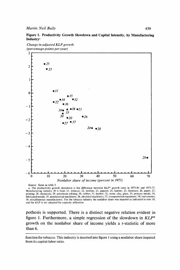
Figure 1. Productivity Growth Slowdown and Capital Intensity, by Manufacturing Industrya

Change in adjusted KLP growth (percentage points per year)

3

. 25 2

*23

0 ~~~*31 0 . 35

*34 032 -22 36

390 .38 21 . 33

30 020 *26 -203

027 *37

24. 028

-3

-4

5 ~~~~~~~~~~~~~~29.

-6 a a A I

0 10 20 30 40 50 60 70 Nonlabor share of income (percent in 1973)

Source: Same as table 2. a. The productivity growth slowdown is the difference between KLP* growth rates in 1973-81 and 1953-73.

Manufacturing industry 20 is food; 21, tobacco; 22, textiles; 23, apparel; 24, lumber; 25, furniture; 26, paper; 27, printing; 28, chemicals; 29, petroleum refining; 30, rubber; 31, leather; 32, stone, clay, glass; 33, primary metals; 34, fabricated metals; 35, nonelectrical machinery; 36, electrical machinery; 37, transportation equipment; 38, instruments; 39, miscellaneous manufacturers. For the tobacco industry the nonlabor share was imputed as indicated in note 19, and the KLP is not adjusted for capacity utilization.

pothesis is supported. There is a distinct negative relation evident in figure 1. Furthermore, a simple regression of the slowdown in KLP* growth on the nonlabor share of income yields a t-statistic of more than 6.

function for tobacco. This industry is inserted into figure 1 using a nonlabor share imputed from its capital-labor ratio.


Figure 2. Productivity Growth Slowdown and Past Productivity Growth, by Manufacturing Industrya

Change in adjusted KLP growth (percentage points per year)

3

*25 2

*23

031 *35

032 034 *22 -36

*21,33 *38 * 30 *39 026 @20

-2 37 027

24.*2

3

-4

5 029

-6 La ., , ,1A 0 0.5 1.0 1.5 2.0 2.5 3.0 3.5 4.0 4.5 5.0 5.5

Adjusted KLP growth in 1953-73 (percent per year) Source: Same as table 2. a. See figure 1, note a.

Figure 2 does reveal a tendency for the industries with rapid adjusted KLP growth in 1953-73 (the ones on the steep portion of the S-curve shown above) to have experienced a larger slowdown: a simple regression shows a negative correlation with a t-statistic of more than 2. But the relation is much weaker than that of figure 1. In a regression with both nonlabor share and pre-1973 growth as independent variables, only the nonlabor share retains statistical significance. The apparel (23), furniture (25), and petroleum refining (29) industries accentuate the


negative correlations in both figures. But even with these three excluded from figure 1, there remains a clear negative correlation. In figure 2 the scatter is basically horizontal without industries 23, 25, and 29. Thus there is little evidence that the process by which technology affects production is captured by the industry cross-sectional model, so that the role of technical change in the productivity slowdown has not been resolved. However, the fact that adjusted KLP slowed in almost all industries does suggest that the slowdown came mainly from sources other than technical change; in this model, a slowdown in technical change would have little effect on the performance of mature industries.

Even though figure 1 is consistent with the hypothesis that capital services have declined, it also reveals that this hypothesis is incomplete. The data imply a positive intercept and a rather steep slope to the line relating the slowdown to the nonlabor share. A more plausible line would have a zero or small negative intercept and be fairly flat, consistent with no acceleration of technical change and a modest rate of decline of the ratio of capital services to capital stock.20 Developments in technology that are industry-specific and not part of the model probably explain this. For example, the development of new adhesives is said to be one reason why furniture has shown accelerating growth, but since this is not accounted for, the result is a rise in the estimated intercept. Energy and regulation may explain why transportation equipment (37), chemicals (28), and petroleum refining (29) have had such large slowdowns. If these missing elements could be incorporated in the analysis, the implied parameter estimates would be more plausible. Despite this shortcoming, however, the key finding remains. The hypothesis of a decline in capital services predicts that the most capital-intensive industries will have been hardest hit. Within manufacturing, that prediction is certainly borne out.

MEASUREMENT PROBLEMS IN THE COMPUTER INDUSTRY

The real production of computers (part of nonelectrical machinery) is not correctly measured. Technological change has been so rapid in the computer industry that the Bureau of Labor Statistics and the Depart-

20. After this paper was completed, Zvi Griliches suggested to me that textiles (22) and apparel (23) and also furniture (25) and lumber (24) should be combined to make two composite industries because the data are not good enough to separate them. His suggestion would improve figure 1 by pulling in the two outliers, (23) and (25).


ment of Commerce have not been able to develop an adequate output price index. Arbitrarily, the price of computers in nominal dollars has been assumed to be roughly constant since the early 1970s. The deflator for office, computing, and accounting machinery (OCAM) was 99.6 in 1971 and 103.0 in 1980. Real gross investment in such machinery was $15.8 billion in 1980 (1972 dollars) and $16.3 billion in current dollars.

No one has a good price index for the OCAM industry but a recent study by Michael McKee has proposed an alternative index that implies that the official value of 103.0 for 1980 might be three to four times too high.21 This would mean that the price of the output of the OCAM industry was declining at over 20 percent a year relative to the price of other producer durables. This is a rather steep decline and represents about the limit of plausibility.

But suppose one accepts the suggested alternative price index. How much difference would that make?

McKee factors in his price index by using 1972 dollars as the appropriate measure of output. He finds that the rapidly declining price implies that the real gross output of the OCAM industry was $57 billion (1972 dollars) in 1980. This compares with the official figures of $15.8 billion and $16.3 billion cited above. McKee points out that adding $41 billion to real goods output in 1980 eliminates any overall productivity slowdown in manufacturing, with room to spare.

There are two problems with this procedure. The first is a technical one. When relative prices change dramatically, the usual method of calculating output in 1972 dollars can quickly become absurd because the weights assigned to each product are soon very far out of line. $57 billion (1972 dollars) would represent over 8 percent of total real goods output in 1980. But in nominal dollars, computers amounted to only 1.4 percent of total goods output. The alternative price index has ballooned not only the growth rate of the OCAM industry, but also its weight in the total. A more appropriate procedure is to use a divisia chain index, dividing goods output into computers and everything else. Using the divisia index and the alternative price index for computers reduces the productivity slowdown in manufacturing by only 0.3 percentage point compared to the slowdown using the official data.

21. Michael J. McKee, "Computer Prices in the National Accounts: Are Our Economic Problems a Computer Error?" (Council of Economic Advisers, 1982).


The second problem with using the alternative price index occurs because computers are capital goods. If the output of computers is being understated, then so is investment and the capital stock-the same issue that arose for productivity in construction. In the short run, an error in measuring computer output will cause KLP to be understated, too, because an extra dollar of computer output adds a full dollar to output immediately, while an extra dollar of capital reduces the estimate of KLP by much less than a dollar. Over time, however, the error in measuring the capital stock becomes cumulatively larger, since computers last more than a year. If computer output is being understated, the KLP slowdown becomes even greater and more puzzling as time goes on.

ENERGY USE IN MANUFACTURING

The effort to economize on energy following its price increases in the 1970s may have caused a decline in the flow of output-producing capital services relative to the measured capital stock, or it may have influenced productivity in other ways. Energy could be economized by reducing energy-intensive operations or by diverting resources to energy conservation from other uses. In the absence of more direct evidence on such responses, I analyzed pre-1973 energy intensity and an estimate of energy conservation actually achieved. I used the recently released data from the Department of Commerce that gives annual energy consumption by two-digit manufacturing industries for detailed types of energy for 1958-77.22 I divided the types of energy consumed into fourteen cate- gories and then calculated a divisia index of energy use for each industry, using expenditure shares as weights.

The importance of energy was assessed by looking at the correlation between energy intensity and the slowdown and by determining how much energy has been saved. Energy intensity was measured by the ratio of expenditure on energy to value added in 1973, both in current dollars. Table 3 gives the energy intensities by industry in percent. There is a statistically significant correlation between the size of the slowdown by industry and energy intensity (a t-statistic of 2.1). But the association is not as strong as for capital intensity.

22. I am grateful to Joseph Correia of the Department of Commerce, Bureau of Industrial Economics, for supplying the data tape and assisting in its use.


Table 3. Productivity Slowdown, Energy Intensity, and Energy Conservation

Rank in Energy Energy productivity Industry and intensity conservation slowdowna classification number (percent)b (ratio)c

1 Petroleum refining (29) 19.84 ... 2 Chemicals (28) 17.45 1.19 3 Lumber (24) 5.24 0.84 4 Printing (27) 2.50 0.63 5 Transportation equipment (37) 1.99 0.47 6 Food (20) 5.14 1.01 7 Paper (26) 10.88 0.85 8 Rubber (30) 4.42 0.52 9 Miscellaneous manufactures (39) 3.18 0.60

10 Primary metals (33) 20.65 0.61 11 Instruments (38) 0.91 0.82 12 Tobacco (21) 0.83 1.01 13 Electrical machinery (36) 2.31 0.62 14 Textiles (22) 5.26 0.74 15 Fabricated metals (34) 2.75 0.58 16 Stone, clay, glass (32) 11.41 0.65 17 Nonelectrical machinery (35) 2.21 0.72 18 Leather (31) 2.60 0.78 19 Apparel (23) 2.48 0.51 20 Furniture (25) 2.52 0.62

Source: Computed by the author as described in the text. a. Based on KLP* slowdown from table 2. Rank 1 is the largest slowdown; rank 20 is the largest acceleration in

productivity growth. b. Expenditure on energy as a percent of value added in 1973, both in current dollars. c. Ratio of energy actually used in 1977 to energy use projected from pre-1973 trends and actual 1977 output.

There were marked trends in energy productivity before 1970, so that to know how much energy has been saved required an estimate of how much energy would have been used with no price increases. The logarithm of energy productivity-the ratio of output (value added in 1972 dollars) to the quantity of energy used-was regressed on a quadratic in time over the 1958-72 period. The fitted value from the equation for 1977 was then taken as the estimate of what energy productivity, and hence energy use, would have been in the absence of subsequent price increases. Energy conservation is measured as the ratio of actual energy use in 1977 to this estimate of what it would have been.

Table 3 gives the resulting measures of conservation by industry.23 The table shows that there was a substantial effort at energy conservation

23. There were discontinuities in the data for petroleum refining that seemed to invalidate the computation of energy use over the full 1958-77 period.


relative to the pre-1973 trends. Energy use in 1977 was below what it would have been, given output, for all industries except three. This shows that energy saving was pervasive and is consistent with the idea that efforts to save energy contributed to the widespread weakness in productivity. There is no correlation, however, between the pattern of energy conservation by industry and the magnitudes of the slowdown by industries.

The fact that a worldwide productivity slowdown began shortly after the price of energy increased in 1973 makes one suspect energy of contributing to the productivity slowdown. And large slowdowns in industries that feel the impact of energy prices, such as public utilities, mining, petroleum refining, chemicals and transportation equipment, strengthen the suspicion. However, the examination here of the detailed energy consumption data by industry does not reinforce that case. These data make energy look more like an accessory and less like the prime suspect. More careful treatment of the behavior of energy productivity before the price increases might change the conclusions, but this is doubtful. The basic data just do not show a pattern of conservation that coincides with the pattern of the slowdown. It is possible that conservation patterns have changed substantially since 1977 or that environmental regulation has affected energy consumption (in the chemical industry, for example). Alternatively energy conservation may be easier in some industries than in others so that differences in the ease of conservation, rather than in the amount of resources devoted to it, may explain the difference in the conservation achieved. But these possibilities remain to be shown.

Effects of Changes in Industry Mix

In this section, I turn to the fourth and final question posed at the beginning of this paper. It has been suggested by William Nordhaus that changes in the shares of output and employment by industry can have important effects on aggregate productivity that are separate from what is happening within the particular industries making up the aggregate.24

24. William D. Nordhaus, "The Recent Productivity Slowdown," BPEA, 3:1972, pp. 493-536.


This argument has also been important from a policy perspective. The importance of changes in industry shares has been cited to support a U.S. industrial policy favoring industries with high productivity levels or rapid growth rates.25

The standard way of estimating industry-mix effects was presented by Nordhaus and can be illustrated with a simple model like the one used earlier. There are n sectors, i = 1, . . ., n. Output and labor input for the ith sector are Qi and Li, respectively. The output of the ith sector is sold at a price ai in the base period, so that total real output for the economy, Q, is given by26

(13) Q = IEiQi.

Then define ALP as average labor productivity for the economy as a whole (Q/E Li), ALPi as the same for the ith sector (1TjQj/Lj), Oi as the share of the ith sector in total output, and Si as the share of the labor input in the ith sector. It follows that the rate of growth in labor productivity is

(14) alp = i ~ alpi + (ALPA dSt (ALP / dt

ALPS dSi = ialpi + E(0i - 6i)alpi + E (AP- 1)di, ALP /dt 9

where Oi is the share in 1972 of the ith sector in total output. The second line follows from the first because the sum of the changes in labor shares is zero. The expression indicates that the rate of growth of labor productivity for the economy as a whole is a weighted average of the rates of growth of the individual sectors with fixed (1972) output weights, plus a term that is positive if the output shares are growing in sectors with above-average rates of labor productivity growth, plus another term that is positive if the labor shares are growing in sectors with above- average levels of labor productivity. The results of decomposing aggregate labor productivity in the way indicated by equation 14 for the private business economy are shown in table 4 for various periods. The final

25. Lester C. Thurow, "Solving the Productivity Problem," and Arnold Packer, "Productivity and Structural Change," in Center for Democratic Policy, Strengthening the Economy: Studies in Productivity (Washington, D.C., 1981), pp. 9-19, 20-27.

26. The overall price level is normalized to equal unity.


term in equation 14 is split into two parts in table 4, the farm sector and the sum of the nonfarm sectors.

The first result to note in table 4 is that the effect of changes in output shares on the overall growth rate of productivity is trivial. The term (0i - O4)alpi is small in all periods, and it actually turned positive after 1973. The simple reason for this outcome is that output shares have not changed that much. Manufacturing produced 30.4 percent of real business output in 1948 and 30.7 percent in 198 1. For the same years, services produced 13.3 percent and 14.8 percent; trade produced 19.5 percent and 21.2 percent. Those three sectors account for two-thirds of business output.27 Of the remainder, communications and public utilities have grown in importance, and agriculture, railroads, and construction have declined in output shares.

These findings may be surprising given that it is frequently alleged that the increased size of stagnant industries has played a major role in the overall productivity story.28 Some people look at employment shares rather than output shares, but this is a misleading procedure. Think of an economy in which 90 percent of the output is produced by an automated industry requiring only one employee. What happens in this automated sector will dominate the aggregate productivity picture, but its employment share is trivial. Others look at total GNP, for which the growth in government and nonbusiness services may well have contributed somewhat to the growth slowdown in aggregate productivity.

The second finding shown in table 4 is that the industry-mix effect associated with movements of labor among sectors with different levels of average labor productivity did apparently contribute to the slowdown in overall growth after 1965. The cessation of favorable mix effects contributed - 0.22 percentage point to a total slowdown of - 0.71 point, with the farm sector alone contributing most of the - 0.22 point.

The contribution of changes in the mix term to the post-1973 slowdown is somewhat smaller and, of course, the slowdown itself is much larger. The term I O1alpi contributes - 1.84 to a total slowdown of - 1.99. Nevertheless, the impact of the winding down of favorable shift effects

27. Data are provided by Elliot S. Grossman. They include allocation of government enterprises output.

28. See William J. Baumol and Edward Wolff, "On the Theory of Productivity and Unbalanced Growth" (New York University, November 1979).

- r - 0 t 0 -

O 00 ))00 00 I

!~~~~~C r- - "C ) CN O o

I-

t Bo (o C oo

0 r r- r, 7

Q~~~~~~C C) C) C)l C) C )o

4 0000- 00

- w 666 66 oo

1-0 o,3 C

0 200? 0?

0 -

0 0

00 00 Z

;* QQ u

.= 1s, i,:> O Oa-, C O O cO :: ,SH~~~~~~~0

.0_

> x,, 3 to:,s,>~GV2

? ~ ~~ 000O0 00 2\~N< 0Ot' ~Cc


from the farm sector alone has about the same absolute contribution to the post-1973 slowdown as it did to the slowdown after 1965.

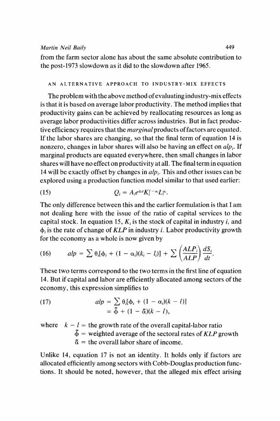
AN ALTERNATIVE APPROACH TO INDUSTRY-MIX EFFECTS

The problem with the above method of evaluating industry-mix effects is that it is based on average labor productivity. The method implies that productivity gains can be achieved by reallocating resources as long as average labor productivities differ across industries. But in fact produc- tive efficiency requires that the marginal products of factors are equated. If the labor shares are changing, so that the final term of equation 14 is nonzero, changes in labor shares will also be having an effect on alpi. If marginal products are equated everywhere, then small changes in labor shares will have no effect on productivity at all. The final term in equation 14 will be exactly offset by changes in alpi. This and other issues can be explored using a production function model similar to that used earlier:

(15) 1=

AiertK-Lx.

The only difference between this and the earlier formulation is that I am not dealing here with the issue of the ratio of capital services to the capital stock. In equation 15, Ki is the stock of capital in industry i, and 4, is the rate of change of KLP in industry i. Labor productivity growth for the economy as a whole is now given by

(16) alp = Oj[jj + (I - ot)(ki - 1I)] + E (ALPi dSt yALP! dt

These two terms correspond to the two terms in the first line of equation 14. But if capital and labor are efficiently allocated among sectors of the economy, this expression simplifies to

(17) alp = , Oj4j + (1 - xi)(k - 1)]

- 4 + (1 - &)(k - 1),

where k - l = the growth rate of the overall capital-labor ratio = weighted average of the sectoral rates of KLP growth

( = the overall labor share of income.

Unlike 14, equation 17 is not an identity. It holds only if factors are allocated efficiently among sectors with Cobb-Douglas production functions. It should be noted, however, that the alleged mix effect arising


from movements of labor among sectors with different average labor productivities has dropped out completely with the assumption that marginal products equate. Rates of KLP growth and the overall rate of capital formation are the only things that matter.

Over a period of years, changes in the allocation of resources among sectors are not infinitesimal and base-year prices fail to reflect the relative values of the different outputs. It is not always clear how these problems will affect measured productivity, but a general presumption is that real output calculated from base-period prices is biased downward by changes in the output mix and in relative prices. For changes over a period of several years, equation 17 would not hold exactly even if the other assumptions of the model were correct.

Another way in which equation 17 may fail to hold is that wage rates may not equalize across industries. For example, in 1980 hourly compensation was $4.53 in farming and $9.43 in the nonfarm business sector.29 It is not certain how much of this wage differential represents inefficiency. The observed wage reflects the return to human capital as well as to labor. Because of unions and other institutional factors, however, it is likely that wage distortions exist and, in particular, much of the above gap between farm and nonfarm wages reflects excess farm labor.

The n-sector model can be modified to allow for unequal wages. Suppose there are two sectors and sector 1 is high-wage, with the ratio of the sector 1 wage to the sector 2 wage given by 13> 1. Then overall labor productivity growth is

(18) alp = 4 + (1 - o)(k- 1) + (1 -)202(-S2),

where s denotes the rate of change in the share of the labor input in the ith sector. If the share of employment is declining in the low-wage sector, this will augment overall labor productivity depending upon the wage differential (1 - 1), and the ratio of the wage bill in sector 2 to total output ((x202).

AN ALTERNATIVE ESTIMATE OF INDUSTRY-MIX EFFECTS

The modeljust developed can provide an alternative way of estimating the importance of mix effects. Consider the following decomposition of labor productivity growth in the private business sector of the economy, where the subscriptf represents the farm sector:

29. Data provided by the Bureau of Labor Statistics.


(19) alp=4+( - + + (1 - o)(k -1) + (a7 - o)(k- 1) + (13 - l)xfOf(-sf) + residual.

This equation is not estimated; instead each term is computed and then the residual is the part of alp left over. The first term, 4), is the weighted average of the KLP growth rates of the major sectors using fixed (1972) output weights. The second term, (+ - )), is positive (negative) if the output shares have been growing (falling) in sectors with high rates of KLP growth (not necessarily high rates of labor productivity growth).

The term (1 - 'a)(k - 1) gives the contribution of capital to labor productivity growth with a fixed (1972) income share coefficient. In a model with Cobb-Douglas functions in individual sectors, the only reason for the factor shares to change is a change in the mix of output. In this case the term ((x - &)(k - 1) is positive if the labor share of income has declined over time, that is, if the profit share of income has risen. If the industry output shares are increasing (decreasing) in sectors with large capital coefficients, a given rate of increase of the capital-labor ratio adds more (less) to labor productivity growth.

In practice, the profit share has fallen somewhat, both overall and within the major sectors of the economy, so that the data do not exactly fit the model. This may result, in part, from mix effects within the major sectors, and in part from an elasticity of substitution different from unity. Thus the fourth term in equation 19 combines the effect of the interaction between output-mix changes and capital accumulation with the effect of changes in the opportunities for capital-labor substitution.

The fifth term attempts to capture the positive contribution to growth resulting from the movement of labor away from farming, where 3 is the ratio of hourly compensation in the nonfarm sector to hourly compensation in the farm sector. This term probably overstates or puts an upper bound on the farm-mix effect because part of the wage differential in fact reflects a human capital differential.

The residual captures all remaining effects, which include the following: (1) efficiency gains or losses resulting from the reallocation of labor within the nonfarm sector, (2) efficiency gains or losses resulting from the reallocation of capital, and (3) measurement effects resulting from the use of base-year prices and errors in the assignment of value added among industries.

Table 5 shows the results of decomposing labor productivity growth according to equation 19, and it has some similarities with and differences


from table 4. It shows that changes in output weights have had a trivial impact on productivity growth. The difference between + and 4 is small in all periods. It actually contributed positively to productivity growth in 1977-81. The term ((x - O'0(k - 1) is even smaller and has had no appreciable effect on productivity growth in any period. The decline in capital share has not been enough to make much difference. These findings parallel those of table 4.

The breakdown into KLP and a capital stock contribution was not made in table 5, but the results could have been anticipated from what has already been discovered about KLP growth by industry. The slowing in the ratio of growth of the capital stock to labor has played a modest role in the slower growth of labor productivity. Still, more than half of the total post-1965 slowdown and three-quarters of the post-1973 slowdown are reflected in the single term, 4.

The measure of the impact of the shift out of farming is smaller in table 5 than in table 4. It does seem that the average productivity approach overstates this shift effect. The residual column actually contributes about the same amount to the two slowdowns as does the farm sector column, and its interpretation is not entirely clear. My own view is that the substantial contribution to growth (0.33 percentage point) during 1948-53 reflects real gains from the reallocation of resources. The negative terms after 1973 probably reflect index number problems. The period from 1973 on was one of substantial relative price changes.

To summarize this section, it is preferable to calculate the effects of changes in output and employment shares from a model based on production functions that assume marginal products are equated, unless there is some specific reason to think otherwise. However, by either this method of calculation or by a method that keeps average productivities unchanged as industry shifts take place, industry-mix effects do not account for much of the slowdown in productivity growth after 1973.

Conclusions

After 1973, labor productivity growth slowed by 2 percentage points in the private business sector of the U.S. economy.30 In the analytical

30. This is reported in table 5 and elsewhere.

ON ~ ~ ~ ~ ~ ~ O

co

_ ~ ~ ? ooo m o

C> ON k )

ri~~~~~~~~~~~r x, X o O o o o o

.o

0~~~~~~~~~~~~~~0

.o

Noor-r--e~ 0e1

c)

< k m o b N- o

3- 0*0*0*0*t 00'e B o o o

*CQ

.E~~~~~~~~~~~~~~~~~~. .. f

* ^

o t C

o) 3 3r- ONO

1- r) Ocr- r-- " 0. E 0 0 C oD

; X W z E 9 8~~~~~II-


framework it was shown that the rate of labor productivity growth is equal to the rate of KLP growth plus the nonlabor share multiplied by the growth rate of the capital-labor ratio. The theory presented in the section on industry-mix effects then derived an aggregate version of this relation and showed in table 5 that - 0.26 percentage point of the total slowdown in labor productivity growth came from a decline in the growth rate of the ratio of capital stock to labor input.

Table 5 also shows that an additional - 0.24 percentage point of the slowdown was caused by various changes in the industry shares of output and employment. The remaining - 1.50 percentage points, about three-quarters of the total slowdown, is attributed to declines in the rates of KLP growth.

This paper examines three possible explanations for the declines in the rates of KLP growth in the major industry groups and in the two- digit manufacturing industries. The first explanation is that weak demand has depressed productivity, and based upon the results reported in table 1 for the major industries, this explanation accounts roughly for a further - 0.22 percentage point of the slowdown.3'

The remaining two suggested explanations of the slowdown in KLP growth were structural-a decline in the rate of technical change and a decline in the capital services ratio. The results in this paper do not reveal how much of the remaining slowdown in the private business sector might be attributable to each of these two and how much is left unexplained.

In earlier work I suggested some reasons why capital services might have declined. I pointed to the market value of corporate capital as an indicator that this had in fact occurred. In this paper I show that a general decline in capital services relative to the capital stock carries a clear prediction that the incidence of the slowdown across industries would be correlated with their capital intensities. For the manufacturing sector, this prediction is fulfilled. suggesting that a decline in capital services has been an important cause of the slowdown.

31. The average effects of the cyclical adjustments in table 1 were computed by forming a weighted average of the differences between the second and third columns. The weights were the 1972 output shares.

Comments and Discussion

William D. Nordhaus: Nobody in this room last year knew that there was going to be an international financial crisis, but I think everybody knew that there was a productivity slowdown. This paper represents another stanza in the profession's epic quest to understand that slowdown. Martin Baily has been one of the crusaders in this quest and, in this paper, reports some of the jewels he brought back from his sacking of the data banks at the Department of Commerce.

As an aside, it appears to me that there may have been some rebound in cyclically adjusted labor productivity growth in the last year and a half or so, with a pickup perhaps from zero to the neighborhood of 1.5 percent a year for nonfarm business. But that is an extremely short period and the slowdown is still a very stubborn and important unresolved problem.

Baily looks at a number of possible contributors to the slowdown. One idea that he does not find much support for is that the rate of fundamental innovation or total factor productivity itself has slowed down over the past twenty years. I have for some time thought that this was a reasonable hypothesis, but admit the evidence for it is flimsy. My suspicion that declining inventiveness may be an important factor rests on declining patent rates, declining R&D rates, and my impression that we have seen fewer fundamental innovations in the past ten or twenty years than in the early postwar period.

I would make a somewhat different cross-sectional test than Baily does in looking for these effects. Assume the innovation process strikes industries randomly, like lightning strikes. A fundamental decline in innovation would mean that there were fewer lightning strikes. In this case, one would see a decline in the variance across industries in the rate

455


of productivity growth. I do not have the slightest idea whether that has happened or not. But the negative correlation through time that Baily looks for can arise from independence of these lightning strikes as well as from a decline in innovation.

Baily has added to the evidence that inadequate investment is not responsible for the productivity slowdown, as does Bosworth in this same volume. I think the issue is fairly well settled, although nobody except for a small circle of academics seems to be aware of the evidence.

The major new result in the paper comes from Baily' s capital intensity hypothesis. The idea is something like the following: the usual treatment of capital productivity or total factor productivity takes capital services as proportional to the capital stock or some variant of that. What if there is a decline in capital productivity so that the ratio of capital services to capital stock declines? If the decline is uniform across industries, those industries that have the highest capital intensity should experience the biggest productivity slowdown. Although Baily does not derive much from his major industry breakdown, I am struck by how much of the relative productivity slowdown across manufacturing industries is ex- plained by their capital intensities in his figure 1. And I have never seen that kind of result before. Looking at the figure, it appears that a doubling of capital intensity is associated with something like a 1.5 percent a year relative deceleration in productivity.

The next point concerns the effect of interindustry shifts in output. There are no major surprises here. Baily confirms the view that shift effects cannot account for much of the productivity slowdown in recent years. Similarly, energy does not explain much of the cross-sectional variation in productivity performance. Again, I find it no surprise that he confirms other work showing energy is not responsible.

Overall, Baily has produced some useful new evidence on the productivity mystery. I am particularly struck by the capital-intensity phenomenon, and would recommend some hard thinking about its significance. Aside from that, I had come to the conclusion, before this paper, that the productivity slowdown is not a proper subject for macroeconomics, and he has not changed my mind. If one wants to discover the source of the slowdown, one has to look at the Boeing 707, the United Mine Workers, economies of scale, speed limits of 55 miles an hour, and kitchen remodelings. Technological change may be too unstable a process to find a representation in a conventional econometric formulation.


General Discussion

Martin Baily agreed with William Nordhaus that looking at the cross- sectional variances of productivity growth in various periods might provide a test of the hypothesis that we are running out of ideas. He reported that the cross-sectional variances of adjusted KLP growth within manufacturing had not fallen after 1973, so the hypothesis was not supported. Baily also pointed out that an explanation of the slowdown that emphasized disaggregation and such specific things as the 55 MPH speed limit would have to account for the coincidence of so many industries and countries slowing down at about the same time.

A number of discussants suggested that the productivity slowdown might have to be investigated at a still more disaggregated level. Robert J. Gordon described two industries with which he was familiar and in which productivity gains had slowed-aircraft equipment and coal-fired power generation equipment. One issue illustrated by both industries is the consequence of running out of technological possibilities. A second issue, illustrated by industries such as air transportation that use aircraft equipment, is that the official statistics understate the productivity slowdown because of unmeasured efficiency improvements in their products through the 1950s and 1960s. Such improvements implicitly raised the true output of the industries in those years compared to the measured output. If unmeasured efficiency improvements have not occurred to the same degree in the 1970s, the mystery of the productivity slowdown only deepens. But William Brainard observed that such unmeasured gains could well be occurring now with the technological revolution in areas like computers and communications.

Alan Blinder suggested it might be especially useful to study industries with homogeneous products. Many industrial products such as enve- lopes, bolts, and coal are virtually identical in 1982 to their counterparts in 1950, so that looking at their production would avoid the kinds of measurement problems Gordon raised. Baily reasoned that such a focus would have a downward bias. Some of the industries with the most standardized outputs, such as the coal industry, have shown the largest productivity declines. And one would expect that the process of innovation would be faster in industries with new and evolving products rather than in industries in which products remain unchanged for three decades.


Despite the absence of any strong cross-sectional relation between energy and productivity in Baily's results, Blinder remained impressed by the fact that the productivity slowdown began in many industries and across many different countries around the time of the first oil price shock. He reasoned that producers in 1973 were probably familiar with alternative production technologies in the neighborhood of technologies then in current use, but were doubtless far less knowledgeable about technologies appropriate to the new energy prices. Even though similar relative prices had been experienced back in the 1950s, knowledge about energy saving technologies had simply "rotted away" from lack of use.

Lawrence Klein also doubted that the energy explanation had been clearly disproven either in this paper or elsewhere. The coincidence of timing described by Blinder was simply too striking to be entirely accidental. Moreover, despite Baily's weak results with industry cross- sections, Klein believed that some of the largest drops in productivity growth have been in energy-intensive industries. He argued that one should look at industry gross output in measuring productivity rather than value added because the latter may be poorly measured as a result of price inflation; moreover, value added does not include the intermediate energy component and should be measured on a gross basis so that energy is included both on the output and input sides of the production relation. Baily agreed that gross output is better in principle, but said that the only available gross output data are heavily contaminated by intra-industry shipments. Klein also disliked Baily's assumption of constant returns to scale in the production process, reasoning that a more general specification of the production technology should be used, particularly in periods when capital utilization fluctuated so widely. Christopher Sims remarked that it was actually quite difficult to determine the energy intensity of an industry because in computing energy inputs one must take into account the energy intensity of all intermediate goods used in an industry's production process.

Barry Bosworth pointed out that, to identify weak productivity since 1973 with unforeseen obsolescence of capital, one would have to hypothesize large and continuing episodes of unforeseen obsolescence, not one major event such as the first OPEC oil price increase. A one- time loss of effective capital after 1973 would not explain the decline in the measured rate of return over the rest of the decade because normal depreciation and retirements would, in any case, have removed much of


that capital from the statistics by 1980. For example, if 25 percent of the stock of equipment became unexpectedly obsolete at the end of 1973, the measured value of total tangible assets in 1980 would be only 2 percent in error. Baily replied that various supply shocks in the 1970s had in fact been continuing or recurrent. For example, OPEC raised oil prices sharply in 1973 and then again in 1979.

Robert Solow observed that "divine providence" would have been the leading candidate to explain the productivity slowdown not so many years ago. While not taken seriously as an explanation today, a variant is worth considering. It is possible that we are now experiencing normal productivity growth, and that for a variety of reasons, including random error, the 1950s and 60s saw above-average productivity growth.

the productivity growth slowdown by industry - … · the productivity growth slowdown by industry...

Documents