the properties of galaxies in supercluster filamentsetheses.bham.ac.uk/986/1/porter07phd.pdfthe...
TRANSCRIPT

The properties of galaxies insupercluster filaments
byScott Clive Porter
A Thesis submitted to
The University of Birmingham
for the degree of
Doctor of Philosophy
Astrophysics and Space Research Group
School of Physics and Astronomy
University of Birmingham
England
October 2006

University of Birmingham Research Archive
e-theses repository This unpublished thesis/dissertation is copyright of the author and/or third parties. The intellectual property rights of the author or third parties in respect of this work are as defined by The Copyright Designs and Patents Act 1988 or as modified by any successor legislation. Any use made of information contained in this thesis/dissertation must be in accordance with that legislation and must be properly acknowledged. Further distribution or reproduction in any format is prohibited without the permission of the copyright holder.

Synopsis
Superclusters appear as large-scale structures in the form of a network of fila-
ments, and can be up to 100 h−1100 Mpc in extent. In this dissertation, we investigate
in detail the spatial structure of the three richest superclusters of galaxies closer to
us then z=0.1.
We investigate the rate of star formation in galaxies at various positions among
the filaments and clusters in the Pisces-Cetus Supercluster. We use an index of star
formation derived from a principal component analysis of optical spectra. We have
shown that galaxies which are members of these filaments, show a steady decline in
star formation rate, from the periphery of a cluster, into the cluster core. However,
on top of this trend, we find a nearly instantaneous enhancement of the rate of star
formation at ∼ 3 h−170 Mpc from its centre. We conclude that the most likely reason
for this sudden enhancement in star formation rate is galaxy-galaxy harassment.
Further work shows that the enhancement in star formation occurs mainly in the
infalling dwarf galaxies (−20 < MB < −17.5) and that there is little evidence
that the tidal effect of the dark matter haloes of the clusters is responsible for the
enhanced star formation.
The results of an anaylsis performed on a larger ensemble of 52 filaments were
consistent with the those from our smaller sample drawn from the Pisces-Cetus
supercluster.
We conclude this study with the analysis of a sample of spectra from the 6dF
redshift survey. In the absence of spectrophotometric calibration, for these galaxies
we were only able to obtain an uncalibrated star formation rate, but we could
examine the effect of correction due to dust extinction, and could separate the star-
forming galaxies from the active galactic nuclei. From our small sample, there was
interesting evidence of enhanced star formation in galaxies at similar distances from
the centres of the clusters in the Shapley Supercluster.

Acknowledgements
Over the course of my PhD I have received help and support from a range of
people, but my foundation of strength has come from my parents as it has throughout
my life. They supported me both financially and emotionally throughout my degree
and PhD and have always encouraged without applying pressure. Without them I
would never have completed this work. I would also like to say a massive thank you
to my supervisor Dr Somak Raychaudhury for his constant support and inspiration.
He has always been able to pull me forwards when everything seemed to be going
wrong and re-light the fires of determination to continue. I am indebted to Philip
Lah for his contribution of 6dF spectroscopic data and Kevin Pimbblet for sharing
with us his work on filaments in the 2dFGRS. I am also grateful to Stuart Aston,
Stephen Fletcher and Robert Satchwell for their support and friendship which helped
pull me through my degree. Going further back I would like to thank my A level
mathematics teachers at Stourbridge College, Shangara Baines and Lhaktar Dhaga.
When others had told me to quit, they believed in me and their efforts, above and
beyond the call of duty, enabled me to continue my education. I would also like to
mention the other inhabitants of G27 and members of the extragalactic group for
their scientific advice and discussions on football and cricket which always lightened
a day of programming. Finally I would like to thank all the members of Astrosoc
over the years and the committee members I served with. They provided a much
needed distraction from the technical side of astrophysics and enabled me to see the
beauty of the Universe I was studying.

Publications
Publications in Refereed Journals
1. The Pisces-Cetus Supercluster a remarkable filament of galaxies in the 2dF
Galaxy Redshift and Sloan Digital Sky surveys: Scott C. Porter and Somak
Raychaudhury, 2005, MNRAS, 364, 1387-1396 (astro-ph/0511050). (This pa-
per is integrated into chapters 3 and 4)
2. Star formation in galaxies along the Pisces-Cetus Supercluster filaments: Scott
C. Porter and Somak Raychaudhury, 2006, MNRAS, accepted, (astro-ph/0612357).
(This paper is integrated into chapter 4)
3. Star formation properties of galaxies in supercluster filaments in the 2dF
Galaxy Redshift Survey: Scott C. Porter, Somak Raychaudhury and Kevin
A. Pimbblet, in preparation. (This paper is integrated into chapter 5) [Kevin
Pimbblet contributed the initial filament catalogue]
Publications in Contributed Conference Proceedings
1. The Pisces-Cetus Supercluster: the largest filament of galaxies in the 2dF-
GRS region, Scott C. Porter and Somak Raychaudhury 2004, abstract in the
proceedings of the RAS National Astronomy Meeting, Milton Keynes, April
2004.
2. Enhanced star formation in group galaxies in the Pisces-Cetus supercluster:
Scott C. Porter and Somak Raychaudhury, 2005, abstract in the proceedings
of the RAS National Astronomy Meeting, Birmingham, April 2005.
3. Star formation properties in Supercluster Filaments: Somak Raychaudhury
and Scott C. Porter, 2005, abstract, Bulletin of the American Astronomical
Society, 207, 177.15

Contents
1 Introduction 1
1.1 Structure formation . . . . . . . . . . . . . . . . . . . . . . . . . . . . 2
1.1.1 The power spectrum . . . . . . . . . . . . . . . . . . . . . . . 3
1.1.2 The growth of perturbations . . . . . . . . . . . . . . . . . . . 4
1.2 Dark matter and cosmological models . . . . . . . . . . . . . . . . . . 5
1.2.1 Hot Dark Matter . . . . . . . . . . . . . . . . . . . . . . . . . 6
1.2.2 Warm Dark Matter . . . . . . . . . . . . . . . . . . . . . . . . 9
1.2.3 Cold Dark Matter with Dark Energy . . . . . . . . . . . . . . 9
1.2.4 Bias . . . . . . . . . . . . . . . . . . . . . . . . . . . . . . . . 10
1.2.5 Peculiar velocities . . . . . . . . . . . . . . . . . . . . . . . . . 10
1.2.6 N-body simulations . . . . . . . . . . . . . . . . . . . . . . . . 11
1.3 The definition of a supercluster . . . . . . . . . . . . . . . . . . . . . 12
1.4 Observational Surveys . . . . . . . . . . . . . . . . . . . . . . . . . . 14
1.4.1 The Two Degree Galaxy Redshift Survey . . . . . . . . . . . . 14
1.4.2 The 2dFGRS Percolation-Inferred Galaxy Group catalogue . . 15
1.4.3 The Six degree Galaxy Survey . . . . . . . . . . . . . . . . . . 16
1.4.4 The Sloan Digital Sky Survey . . . . . . . . . . . . . . . . . . 17
1.4.5 Super COSMOS . . . . . . . . . . . . . . . . . . . . . . . . . . 18
1.5 Cosmology in this thesis . . . . . . . . . . . . . . . . . . . . . . . . . 18
1.6 Thesis Outline . . . . . . . . . . . . . . . . . . . . . . . . . . . . . . . 19
2 Star formation in galaxies 20
2.1 Star formation as a function of time . . . . . . . . . . . . . . . . . . . 20
2.2 Star formation as a function of environment . . . . . . . . . . . . . . 22
v

Contents vi
2.3 Star formation indicators . . . . . . . . . . . . . . . . . . . . . . . . . 23
2.3.1 Recombination lines of Hydrogen . . . . . . . . . . . . . . . . 23
2.3.2 Ultraviolet continuum emission from hot stars . . . . . . . . . 25
2.3.3 Infrared thermal emission . . . . . . . . . . . . . . . . . . . . 26
2.3.4 X-ray Luminosity . . . . . . . . . . . . . . . . . . . . . . . . . 27
2.4 Star formation in interacting galaxies . . . . . . . . . . . . . . . . . . 27
2.4.1 Star formation mechanisms . . . . . . . . . . . . . . . . . . . 27
2.4.2 Environmental influences . . . . . . . . . . . . . . . . . . . . . 29
2.5 A star formation index from 2dFGRS spectra: the η parameter . . . . 33
2.5.1 The Principal Component Analysis . . . . . . . . . . . . . . . 33
2.5.2 Relationships with other parameters . . . . . . . . . . . . . . 34
2.5.3 Separating the star-forming and non star-forming populations 38
3 Supercluster structure 42
3.1 Minimal spanning tree supercluster structure . . . . . . . . . . . . . . 42
3.1.1 The Pisces-Cetus supercluster . . . . . . . . . . . . . . . . . . 43
3.1.2 The Horologium-Reticulum Supercluster . . . . . . . . . . . . 46
3.1.3 The Shapley supercluster . . . . . . . . . . . . . . . . . . . . . 52
3.2 Mean redshift and velocity dispersion . . . . . . . . . . . . . . . . . . 54
3.2.1 Models of Surface brightness . . . . . . . . . . . . . . . . . . . 56
3.3 Virial mass estimates . . . . . . . . . . . . . . . . . . . . . . . . . . . 69
3.4 A lower limit to the Mass of the Superclusters . . . . . . . . . . . . . 71
3.4.1 Pisces-Cetus supercluster . . . . . . . . . . . . . . . . . . . . . 71
3.4.2 Horologium-Reticulum supercluster . . . . . . . . . . . . . . . 72
3.4.3 Shapley supercluster . . . . . . . . . . . . . . . . . . . . . . . 73
3.5 Conclusions . . . . . . . . . . . . . . . . . . . . . . . . . . . . . . . . 73
4 Star formation in the Pisces-Cetus supercluster 76
4.1 Introduction . . . . . . . . . . . . . . . . . . . . . . . . . . . . . . . . 76
4.2 Star formation within Pisces-Cetus supercluster filaments . . . . . . . 77
4.2.1 Filament membership . . . . . . . . . . . . . . . . . . . . . . . 77
4.2.2 Star formation along the A2734-A2800 filament . . . . . . . . 80

Contents vii
4.2.3 Star formation properties of galaxies in all three filaments
combined . . . . . . . . . . . . . . . . . . . . . . . . . . . . . 82
4.2.4 Star formation in high and low velocity dispersion clusters . . 84
4.2.5 Star formation in giant and dwarf galaxies . . . . . . . . . . . 87
4.2.6 Star formation in Groups . . . . . . . . . . . . . . . . . . . . . 88
4.2.7 Welch’s test results . . . . . . . . . . . . . . . . . . . . . . . . 91
4.3 Discussion . . . . . . . . . . . . . . . . . . . . . . . . . . . . . . . . . 93
4.4 Conclusions . . . . . . . . . . . . . . . . . . . . . . . . . . . . . . . . 96
5 Star formation in 2dFGRS filaments 98
5.1 Introduction . . . . . . . . . . . . . . . . . . . . . . . . . . . . . . . . 98
5.2 The filament catalogue . . . . . . . . . . . . . . . . . . . . . . . . . . 99
5.3 The samples . . . . . . . . . . . . . . . . . . . . . . . . . . . . . . . . 99
5.3.1 Filament selection . . . . . . . . . . . . . . . . . . . . . . . . . 99
5.4 Star formation properties . . . . . . . . . . . . . . . . . . . . . . . . . 103
5.4.1 Properties of galaxies in the field . . . . . . . . . . . . . . . . 103
5.4.2 Star formation in galaxies belonging to filaments . . . . . . . . 104
5.4.3 Star formation in giant and dwarf galaxies . . . . . . . . . . . 107
5.4.4 Star formation in short and long filaments . . . . . . . . . . . 108
5.4.5 Star formation in groups . . . . . . . . . . . . . . . . . . . . . 108
5.4.6 Welch’s test results . . . . . . . . . . . . . . . . . . . . . . . . 110
5.5 Star formation in the PIM04 sample filaments . . . . . . . . . . . . . 112
5.5.1 Star formation within the filaments . . . . . . . . . . . . . . . 113
5.5.2 Star formation within giants and dwarfs . . . . . . . . . . . . 114
5.5.3 Star formation in groups . . . . . . . . . . . . . . . . . . . . . 115
5.6 Conclusions . . . . . . . . . . . . . . . . . . . . . . . . . . . . . . . . 118
6 Star formation in the Shapley supercluster 123
6.1 Introduction . . . . . . . . . . . . . . . . . . . . . . . . . . . . . . . . 123
6.2 Spectroscopic data . . . . . . . . . . . . . . . . . . . . . . . . . . . . 125
6.2.1 Removal of AGN . . . . . . . . . . . . . . . . . . . . . . . . . 127
6.2.2 Stellar absorption . . . . . . . . . . . . . . . . . . . . . . . . . 129

Contents viii
6.2.3 Flux calculations . . . . . . . . . . . . . . . . . . . . . . . . . 130
6.2.4 Dust attenuation . . . . . . . . . . . . . . . . . . . . . . . . . 131
6.2.5 Aperture correction . . . . . . . . . . . . . . . . . . . . . . . . 132
6.2.6 SFR calculation . . . . . . . . . . . . . . . . . . . . . . . . . . 132
6.3 Samples of galaxies in various environments . . . . . . . . . . . . . . 133
6.4 SFR as a function of distance from a cluster . . . . . . . . . . . . . . 136
6.5 Fraction of starburst galaxies . . . . . . . . . . . . . . . . . . . . . . 137
6.6 Fraction of passive galaxies . . . . . . . . . . . . . . . . . . . . . . . . 137
6.7 Conclusions . . . . . . . . . . . . . . . . . . . . . . . . . . . . . . . . 138
7 Conclusions 141
7.1 Summary of main results . . . . . . . . . . . . . . . . . . . . . . . . . 141
7.2 Future work . . . . . . . . . . . . . . . . . . . . . . . . . . . . . . . . 143
Bibliography 145
A Optical Surface brightness fits to clusters (P-C) 160
B Optical Surface brightness fits to clusters (H-R) 163
C Optical Surface brightness fits to clusters (S) 168
D X-ray analysis of the Pisces-Cetus supercluster 172
D.1 X-Ray observations . . . . . . . . . . . . . . . . . . . . . . . . . . . . 172
D.1.1 ROSAT archival pointed observations . . . . . . . . . . . . . . 172
D.1.2 Rosat all-sky Survey and Einstein IPC observations . . . . . . 173
D.1.3 The LX–σ relation . . . . . . . . . . . . . . . . . . . . . . . . 173
D.1.4 Pisces-Cetus supercluster results . . . . . . . . . . . . . . . . . 175
E The 2dFGRS “clean sample” of filaments 178

List of Figures
1.1 The power spectrum of density perturbations as a function of scale
size. . . . . . . . . . . . . . . . . . . . . . . . . . . . . . . . . . . . . 7
1.2 The distribution of dark matter in the millennium simulation. . . . . 12
1.3 The galaxy redshift distribution for the 2dFGRS survey. . . . . . . . 15
2.1 The principle components used in generating the 2dFGRS η parameter. 35
2.2 Distribution η versus galaxy morphology. . . . . . . . . . . . . . . . . 36
2.3 Correlation between η and the equivalent width of the Hα emission
line. . . . . . . . . . . . . . . . . . . . . . . . . . . . . . . . . . . . . 36
2.4 Distribution of η versus the birth rate. . . . . . . . . . . . . . . . . . 38
2.5 A histogram of the η for 2dFGRS galaxies with z < 0.1 . . . . . . . . 39
2.6 Composite fit to the η distribution. . . . . . . . . . . . . . . . . . . . 40
2.7 Individual fits to the η distribution. . . . . . . . . . . . . . . . . . . . 40
3.1 Pisces-Cetus supercluster, clusters of galaxies with minimal spanning
tree links. . . . . . . . . . . . . . . . . . . . . . . . . . . . . . . . . . 45
3.2 Pisces-Cetus supercluster 2dFGRS and SDSS galaxies . . . . . . . . . 46
3.3 Pisces-Cetus supercluster, SuperCOSMOS galaxies. . . . . . . . . . . 47
3.4 Pisces-Cetus SuperCOSMOS galaxy Density contours . . . . . . . . . 48
3.5 Pisces-Cetus supercluster, clusters of galaxies in R.A.-redshift space . 48
3.6 Pisces-Cetus supercluster wedge diagram of 2dFGRS galaxies. . . . . 49
3.7 Pisces-Cetus supercluster, clusters of galaxies in Dec.-redshift space . 49
3.8 Horologium-Reticulum supercluster, clusters of galaxies with minimal
spanning tree links. . . . . . . . . . . . . . . . . . . . . . . . . . . . . 50
3.9 Horologium-Reticulum supercluster ZCAT galaxies. . . . . . . . . . . 51
ix

List of Figures x
3.10 Horologium-Reticulum supercluster, clusters of galaxies in R.A.-redshift
space. . . . . . . . . . . . . . . . . . . . . . . . . . . . . . . . . . . . 51
3.11 Horologium-Reticulum supercluster Wedge plot of ZCAT galaxies. . . 52
3.12 Shapley supercluster, clusters of galaxies with minimal spanning tree
links. . . . . . . . . . . . . . . . . . . . . . . . . . . . . . . . . . . . . 53
3.13 Shapley supercluster NED galaxies. . . . . . . . . . . . . . . . . . . . 53
3.14 Shapley supercluster, clusters of galaxies in R.A.-redshift space . . . . 54
3.15 Pisces-Cetus supercluster, galaxy cluster colour magnitude relation. . 60
3.16 Pisces-Cetus supercluster galaxy cluster radial velocity histograms. . 65
3.17 Horologium-Reticulum supercluster galaxy cluster radial velocity his-
tograms. . . . . . . . . . . . . . . . . . . . . . . . . . . . . . . . . . . 66
3.18 Shapley supercluster galaxy cluster radial velocity histograms 1. . . . 67
3.19 Shapley supercluster galaxy cluster radial velocity histograms 2. . . . 68
4.1 Pisces-Cetus 2dFGRS supercluster galaxies. . . . . . . . . . . . . . . 78
4.2 Pisces-Cetus supercluster, clusters of galaxies in the 2dFGRS region. 78
4.3 Three filaments of galaxies in the Pisces-Cetus supercluster. . . . . . 79
4.4 2dFGRS galaxies for the galaxy cluster Abell 2734 . . . . . . . . . . . 80
4.5 Mean η as a function of the distance from Abell 2734. . . . . . . . . . 81
4.6 Star forming and passive galaxy distribution for Abell 2800. . . . . . 82
4.7 Star forming and passive galaxy distribution for Abell 2734. . . . . . 83
4.8 Mean η as function of the distance from the nearest cluster. . . . . . 84
4.9 Histograms of η in each distance bin. . . . . . . . . . . . . . . . . . . 85
4.10 Mean η as a function of the distance from the nearest low or high σ
cluster. . . . . . . . . . . . . . . . . . . . . . . . . . . . . . . . . . . . 86
4.11 Mean η in giant or dwarf galaxies as function of distance from the
nearest cluster. . . . . . . . . . . . . . . . . . . . . . . . . . . . . . . 87
4.12 Spatial distribution of giant and dwarf filament galaxies. . . . . . . . 88
4.13 Mean η of group or non-group galaxies as a function of distance from
the nearest cluster . . . . . . . . . . . . . . . . . . . . . . . . . . . . 90
4.14 Mean η of filament or field group galaxies as a function of distance
from the nearest cluster . . . . . . . . . . . . . . . . . . . . . . . . . 90

List of Figures xi
4.15 Histograms of richness and velocity dispersion for group galaxy samples. 91
5.1 Mean η as function of distance from the nearest cluster for the entire
2dFGRS. . . . . . . . . . . . . . . . . . . . . . . . . . . . . . . . . . . 104
5.2 Mean η as function of distance from the nearest cluster. . . . . . . . . 105
5.3 Histograms of η in each of the 8 distance bins. . . . . . . . . . . . . . 106
5.4 Mean η of giant or dwarf galaxies as a function of distance from the
nearest cluster. . . . . . . . . . . . . . . . . . . . . . . . . . . . . . . 107
5.5 Mean η as function of distance from the nearest cluster for long and
short filaments . . . . . . . . . . . . . . . . . . . . . . . . . . . . . . 109
5.6 Mean η of group or non-group galaxies as a function of distance from
the nearest cluster. . . . . . . . . . . . . . . . . . . . . . . . . . . . . 111
5.7 Mean η of filament and field group galaxies as a function of distance
from the nearest cluster. . . . . . . . . . . . . . . . . . . . . . . . . . 112
5.8 Histograms of richness and velocity dispersion for group galaxy samples.113
5.9 Mean η as function of distance from the nearest cluster (PIM04a). . . 115
5.10 Mean η as function of distance from the nearest cluster (PIM04b). . . 116
5.11 Histograms of η within each distance bin. . . . . . . . . . . . . . . . . 117
5.12 Mean η in giant or dwarf galaxies as function of distance from the
nearest cluster. . . . . . . . . . . . . . . . . . . . . . . . . . . . . . . 118
5.13 Mean η in group and non-group galaxies as a function of distance
from nearest cluster. . . . . . . . . . . . . . . . . . . . . . . . . . . . 119
5.14 Mean η in filament and field group galaxies as a function of distance
from nearest cluster. . . . . . . . . . . . . . . . . . . . . . . . . . . . 120
6.1 Example spectra of a 6dF starburst galaxy. . . . . . . . . . . . . . . . 126
6.2 Example spectra of a 6dF passive galaxy. . . . . . . . . . . . . . . . . 126
6.3 Example spectra of a 6dF AGN galaxy. . . . . . . . . . . . . . . . . . 127
6.4 BPT diagram of Shapley region galaxies. . . . . . . . . . . . . . . . . 129
6.5 Histogram of the uncalibrated SFR of galaxies in the Shapley region 1.134
6.6 Histogram of the uncalibrated SFR of galaxies in the Shapley region 2.135

List of Figures xii
6.7 Mean uncalibrated star formation rate as a function of distance from
the nearest cluster. . . . . . . . . . . . . . . . . . . . . . . . . . . . . 136
6.8 Fraction of starburst galaxies as a function of distance from a cluster 138
6.9 Fraction of passive galaxies as a function of distance from a cluster. . 139
A.1 Surface brightness profiles for A0014, A0027 and A0074. . . . . . . . 160
A.2 Surface brightness profiles for A0085, A0086 and A0087. . . . . . . . 161
A.3 Surface brightness profiles for A0114, A0117 and A0126. . . . . . . . 161
A.4 Surface brightness profiles for A0133, A0151 and A2660. . . . . . . . 161
A.5 Surface brightness profiles for A2683, A2716 and A2734. . . . . . . . 162
A.6 Surface brightness profiles for A2800, A2824, and A4053. . . . . . . . 162
A.7 Surface brightness profiles for A2794, S1136 and S1155. . . . . . . . . 162
B.1 Surface brightness profiles of A2988, A3004 and A3009. . . . . . . . 163
B.2 Surface brightness profiles of A3074, A3078 and A3089. . . . . . . . . 164
B.3 Surface brightness profiles of A3093, A3098 and A3100. . . . . . . . . 164
B.4 Surface brightness profiles of A3104, A3106 and A3109. . . . . . . . . 164
B.5 Surface brightness profiles of A3110, A3111 and A3112. . . . . . . . . 165
B.6 Surface brightness profiles of A3116, A3120 and A3122. . . . . . . . . 165
B.7 Surface brightness profiles of A3123, A3125 and A3128. . . . . . . . . 165
B.8 Surface brightness profiles of A3133, A3135 and A3140. . . . . . . . . 166
B.9 Surface brightness profiles of A3145, A3158 and A3164. . . . . . . . . 166
B.10 Surface brightness profiles of A3202, A3225 and A3266. . . . . . . . . 166
B.11 Surface brightness profile of A3312 . . . . . . . . . . . . . . . . . . . 167
C.1 Surface brightness profiles of A1631, A1644 and A1709. . . . . . . . . 168
C.2 Surface brightness profiles of A1736, A3528N and A3528S. . . . . . . 169
C.3 Surface brightness profiles of A3530, A3532 and A3546. . . . . . . . . 169
C.4 Surface brightness profiles of A3552, A3555 and A3556. . . . . . . . . 169
C.5 Surface brightness profiles of A3558, A3559 and A3560. . . . . . . . . 170
C.6 Surface brightness profiles of A3562, A3564 and A3566. . . . . . . . . 170
C.7 Surface brightness profiles of A3568, A3570 and A3571. . . . . . . . . 170
C.8 Surface brightness profiles of A3575, A3577 and A3578. . . . . . . . . 171

List of Figures xiii
C.9 Surface brightness profiles of SC1327 and SC1329. . . . . . . . . . . . 171
D.1 (Top row) X-ray contours from pointed ROSAT PSPC observations,
superposed on optical (Blue) DSS images of the clusters Abell 85,
Abell 133 and Abell 2734. (Middle row) Similar images of Abell 14
(RASS), Abell 74 & Abell 117 (Einstein IPC), Abell 151 (RASS), and
(Bottom row) of Abell 2716, Abell 2794, Abell 2800, and Abell S1136
(all RASS). . . . . . . . . . . . . . . . . . . . . . . . . . . . . . . . . 174
D.2 The relationship between Lx and σ for Pisces-Cetus supercluster clus-
ters with available X-ray literature data. . . . . . . . . . . . . . . . . 176
E.1 Galaxy position, mean η and mean percentage of passive galaxies in
the 2dFGRS filament sample batch 1. . . . . . . . . . . . . . . . . . . 178
E.2 Galaxy position, mean η and mean percentage of passive galaxies in
the 2dFGRS filament sample batch 2. . . . . . . . . . . . . . . . . . . 179
E.3 Galaxy position, mean η and mean percentage of passive galaxies in
the 2dFGRS filament sample batch 3. . . . . . . . . . . . . . . . . . . 180
E.4 Galaxy position, mean η and mean percentage of passive galaxies in
the 2dFGRS filament sample batch 4. . . . . . . . . . . . . . . . . . . 181
E.5 Galaxy position, mean η and mean percentage of passive galaxies in
the 2dFGRS filament sample batch 5. . . . . . . . . . . . . . . . . . . 182
E.6 Galaxy position, mean η and mean percentage of passive galaxies in
the 2dFGRS filament sample batch 6. . . . . . . . . . . . . . . . . . . 183
E.7 Galaxy position, mean η and mean percentage of passive galaxies in
the 2dFGRS filament sample batch 7. . . . . . . . . . . . . . . . . . . 184
E.8 Galaxy position, mean η and mean percentage of passive galaxies in
the 2dFGRS filament sample batch 8. . . . . . . . . . . . . . . . . . . 185
E.9 Galaxy position, mean η and mean percentage of passive galaxies in
the 2dFGRS filament sample batch 9. . . . . . . . . . . . . . . . . . . 186
E.10 Galaxy position, mean η and mean percentage of passive galaxies in
the 2dFGRS filament sample batch 10. . . . . . . . . . . . . . . . . . 187

List of Figures xiv
E.11 Galaxy position, mean η and mean percentage of passive galaxies in
the 2dFGRS filament sample batch 11. . . . . . . . . . . . . . . . . . 188
E.12 Galaxy position, mean η and mean percentage of passive galaxies in
the 2dFGRS filament sample batch 11. . . . . . . . . . . . . . . . . . 189

List of Tables
3.1 Clusters belonging to the Pisces-Cetus Supercluster . . . . . . . . . . 57
3.2 Clusters belonging to the Horologium-Reticulum Supercluster . . . . 58
3.3 Clusters belonging to the Shapley Supercluster . . . . . . . . . . . . 59
4.1 Virial radii for Pisces-Cetus filament clusters . . . . . . . . . . . . . 83
4.2 Welch’s test results for Pisces-Cetus filaments . . . . . . . . . . . . . 92
5.1 Filament type classification in the PIM04 sample . . . . . . . . . . . 100
5.2 Filament information for the 52 visually selected sample. . . . . . . . 101
5.3 Welch’s test results for “clean sample” filaments . . . . . . . . . . . 112
xv

Chapter 1
Captain James Cook: “I had ambition not only to go farther than any man had ever
been before, but as far as it was possible for a man to go.”
Introduction
Throughout history humans have become more and more aware of the universe in
which they live. Boundaries have moved beyond the hunting grounds of ancient
times, expanded beyond the horizon by explorers who dared to go where “here be
dragons” marked the map. Today we have gone beyond the bounds of our little
blue planet and out into the depths of space. Our vision has advanced out beyond
our solar system, out through the billions of stars of the Milky Way, to gaze upon
Andromeda and the other galaxies that form the local group. Then even further we
are drawn out into a universe of other groups of galaxies, huge clusters of galaxies
and a massive network of filaments linking them all together. Finally we arrive at
superclusters of galaxies. These are massive chains of clusters of galaxies linked by
filaments of galaxy groups and individual galaxies.
The term supercluster has been used to denote various entities in literature (see
§ 1.3). However, in this thesis we define the term to denote Large-scale structures
that are much larger than the virial radii of individual rich clusters (>∼10 h−170 Mpc).
Observations and simulations of the large-scale structure of the Universe have
revealed the presence of a network of filaments and voids in which most galaxies
seem to be found (Zucca et al., 1993; Einasto et al., 1994; Jenkins et al., 1998). This
implies that that the Universe is not homogeneous on scales below ∼ 100 h−170 Mpc
(Bharadwaj, Bhavsar, & Sheth, 2004; Shandarin, Sheth, & Sahni, 2004), which is the
scale of the largest common structures of galaxies, though the discovery of structures
1

1.1. Structure formation 2
far larger than these have been claimed (e.g., Brand et al., 2003; Miller et al., 2004).
Perturbations on the scale of superclusters are likely to still be in a linear growth
regime and have not yet reached equilibrium, or to have only recently left the linear
growth regime. If this is the case they have yet to condense out of the Hubble
expansion and can be analytically tractable containing valuable information about
the processes that occurred during their formation. Superclusters are an essential
tool to study the largest-scale density perturbations that have given rise to structure
in the Universe (e.g., Bahcall, 2000). They can be useful in quantifying the the
high-end mass function of collapsing systems and ratio of mass to light on the
largest scales, thus being useful in discriminating between dark matter and structure
formation models (e.g., Kolokotronis, Basilakos, & Plionis, 2002; Bahcall, 1988).
1.1 Structure formation
When the universe was much younger than it is now it was smoother and denser.
Superposed on this smooth background were small fluctuations in the density of
matter and the temperature of the Cosmic Microwave Background (CMB). Accord-
ing to the most popular current theory, initial Gaussian density perturbations in
the primordial universe lead to the formation of structure on different scales as the
universe expanded. The linear theory of gravitational instability shows that density
perturbations grow at best in proportion to the expansion factor of the universe. As
the universe has expanded by a factor of approximately 1000 since the decoupling of
radiation and matter at recombination, density perturbations can only have grown
by a factor of about 1000 since this time. Therefore, the fluctuations should be de-
tectable as small-scale anisotropies in the cosmic microwave background radiation.
This is indeed the case and such anisotropies have been observed by COBE (Smoot
et al., 1992) and more recently the Wilkinson Microwave Anisotropy Probe, WMAP
(Bennett et al., 1997), which used differential microwave radiometers to measure
temperature differences between two points on the sky.

1.1. Structure formation 3
1.1.1 The power spectrum
The cosmological density perturbations or matter overdensities are specified by the
quantity:
δ(x) =ρ(x) − 〈ρ〉
〈ρ〉 , (1.1)
where 〈ρ〉 is the mean density of the universe and ρ(x) is the mass density at position
x.
These spherically overdense regions in the otherwise uniform density universe
will start off decreasing in density at almost the same rate as the rest of the uni-
verse, following linear theory. However, the density gradually stops decreasing and
then starts to increase radically when a critical density is reached. For δ(x) ≪ 1,
the region is in the linear regime and it is possible to analytically model the collapse.
However, for δ(x) & 1 the collapse is in the non-linear regime and becomes too com-
plicated to model analytically and numerical simulations are needed. Superclusters
have been shown to have overdensities of the order of 2 or 3 (e.g., Fabian, 1991;
Fleenor et al., 2005) over scales of larger than 20 h−170 Mpc and will therefore have
only recently have left the linear regime.
Fluctuations in the CMB
The fluctuations in the smooth background must have been created by some kind
of mechanism. The only mechanism which fits with todays observations is inflation,
which refers to a period of exponential expansion of the universe which occurred
soon after the Big Bang (e.g., Albrecht et al., 1982). This process solves two major
problems, that of the flatness problem and the horizon problem. The rapid inflation
of the universe would have smoothed out spacetime allowing the flat universe we see
today. At the same time it explains how regions that are on opposite sides of the
universe today could once have been close enough to have been in communication
allowing for their almost identical CMB conditions. It also allows for seed fluctua-
tions for galaxy formation to have originated from quantum fluctuations that were

1.1. Structure formation 4
then inflated to a macroscopic scale.
1.1.2 The growth of perturbations
The initial Gaussian density perturbations are assumed to have a power-law spec-
trum,
Pi(k) = Akn, (1.2)
where n is the spectral index and k = 2π/L, where L is the size of the perturbation.
Zel’Dovich (1970) approximated the perturbations to be scale invariant or grow
at the same rate as the universe. This led to the Harrison-Zeldovich spectrum, with
n = 1,
P (k) ∝ k. (1.3)
Recent observations by WMAP, have shown the actual value of n in a flat Λ dom-
inated universe, to be remarkably close to the Harrison-Zeldovich approximation
with a value of 0.99 ± 0.04 (Spergel et al., 2003).
The power spectrum at any given time depends on this initial power spectrum
and the transfer function which describes how the initial power spectrum is mod-
ified over time by the physical processes present in the universe. Thus the power
spectrum at a given time in its dimensionless form is described by,
∆2(k) = kn+3 T 2(k, t), (1.4)
where T (k, t) is the transfer function. The amplitude of the perturbations will
continue to grow with time with the shape of the initial spectrum being maintained
in the linear regime. When δ approaches unity on a scale of size L the region
collapses and becomes non-linear, where ρ = ρ0(1 + δ), ρ being the density of the
region and ρ0 the mean density of the universe.

1.2. Dark matter and cosmological models 5
The Press-Schechter formalism
As mentioned above, the non-linear phases of collapse of the matter are too com-
plex to allow completely analytic solutions. Press & Schechter (1974) created a
simplified analytic approach where structure has formed hierarchically from initial
Gaussian fluctuations. They adopted initially overdense regions that would expand
at the same rate as the density of the rest of the universe until z approaches zvir,
the redshift at which the region starts to collapse and becomes virialised. At this
time the region will start to free fall until it collapses to a point. They formulate an
equation which tracks the evolution of the density across regions containing a mass
M on average. This results in an analytical solution where the form of the mass
distribution remains constant, even as the scale of the collapsing objects increases.
This is shown in Eq. 1.5 which defines the fraction of mass fg that is in virialised
structures exceeding mass M at a given redshift.
fg(M, z) = erfc
[
(1 + z)δc√2σ(M, 0)
]
, (1.5)
where erfc is a complementary error function, δc is the critical overdensity and σ is
the r.m.s mass fluctuation over the spherical region containing the mass M
1.2 Dark matter and cosmological models
It has now become obvious that that the luminous matter in the universe only makes
up a very small percentage of the mass in the universe. Observations as far back as
1933 (Zwicky, 1933) showed that the coma cluster had insufficient mass to explain
the velocity dispersion of the galaxies. Further evidence came in the form of the
rotation curves of galaxies. Rubin & Ford (1970) showed that rather than rising to
a peak velocity then dropping as predicted the rotation curve of Andromeda was
in fact flat out to large radii. This has been confirmed for many other galaxies
of varying morphology. More recently X-ray derived masses of clusters of galaxies
and those from gravitational lensing have confirmed the presence of an excess of
mass over that which can be explained from optical observations. The additional
1.2. Dark matter and cosmological models 6
missing mass is referred to as dark matter. Dark matter plays an important role in
the formation of structure as its gravitational influence dominates that of the other
components for most of the life of the universe. It is therefore essential to understand
the properties, amount and distribution of dark matter before large scale structure
can be explained. Dark matter is the dominant influence on the form that the
transfer function and hence the power spectrum described by Eq. 1.4 takes.
A possible candidate for dark matter is massive astrophysical compact halo ob-
jects (MACHOs) such as brown dwarfs and neutron stars. These like the luminous
matter in the universe are baryonic. However, due to constraints on the contri-
bution of baryons to the critical density Ωb imposed by Big Bang Nucleosynthe-
sis (e.g., Burles, Nollett, & Turner, 2001) only a small fraction can be baryonic
(Ωbh2 = 0.020 ± 0.002). Therefore, models were proposed that incorporated non-
baryonic matter in structure formation.
Each of the model types results in a unique form of the power spectrum which
in turn, if correct should describe the universe that we observe today. Examples of
the forms taken by two possible models are shown in Fig. 1.1. The actual power
spectrum of the universe can be found by using the two point correlation function
of galaxies in large scale galaxy surveys, e.g., the APM Galaxy survey (Maddox et
al., 1990) and compared with dark matter models.
1.2.1 Hot Dark Matter
Hot dark matter (HDM) consists of particles that decouple when relativistic. These
particles have a number density roughly equal to that of the microwave background
photons. To remain relativistic for longer periods requires their masses to be less
than ≈ 100 eV. A major advantage of HDM is that it has a definite candidate
in the neutrino which had been suggested to oscillate from one species to another
and hence have non-zero mass (Fukuda et al., 1998). The major problem with
HDM is that in the early universe most of the matter density would have been due
to neutrinos. At this time their speeds would have been too great to be caught
in any overdense regions. Therefore, density fluctuations could only appear after
the universe had expanded enough to let the neutrinos cool and slow down. This

1.2. Dark matter and cosmological models 7
Figure 1.1: The power spectrum of density perturbations as a function of scale size for the
standard HDM and CDM models. (White, 2006). (§1.2)
means that the HDM model would have insufficient power on small scales, i.e., less
small scale structure than that observed (e.g., White, Frenk, & Davis, 1983; White,
Davis, & Frenk, 1984; Zeng & White, 1991). This can be seen in Fig. 1.1 where
the HDM peaks for values of approximately k = 0.1 which corresponds to scales of
L ∼ 10 h−1 Mpc. For scales smaller than 10 h−1 Mpc the HDM model rapidly loses
power and predicts no structures at scales of a few h−1 Mpc or less, excluding galaxy
size structures at the current epoch. The power spectrum changes over time, with
structures forming when a certain threshold of power is exceeded. It can be seen
that the first part of the HDM model to pass a threshold will be at its peak value,
at approximately k = 0.1 and so structures of approximately 10 Mpc will be formed
first. At all times there will be more large scale structure due to the gradual slope
towards low values of k, compared with the steep slope at higher values of k. Thus
HDM is a top down model with larger structures forming first.
Cold Dark Matter
Cold dark matter dominated universes (CDM) have been extensively modelled with
the use of N-body simulations and show a bottom-up structure formation (e.g.,
Peebles, 1982). The most likely candidates for non-baryonic CDM are Weakly in-

1.2. Dark matter and cosmological models 8
teracting massive particles (WIMPS) such as neutralinos, gravitinos, photinos and
higgsinos predicted by supersymmetric theories. Structure grows out of Gaussian
fluctuations with the scale invariant spectrum proposed by Harrison and Zeldovich
, see equation (1.3). The perturbations in the CDM begin to grow at the epoch of
matter-radiation equality but are unstable prior to decoupling. Only after recombi-
nation can the perturbations in the baryons begin to grow by falling into the CDM
potential wells. As material continues to flow into the density fluctuation, the fluc-
tuation continues to grow in size and accrete more matter. Galaxies are eventually
made by the coalescence of larger and larger clumps of matter, and later clusters
and superclusters of galaxies form as the gravitational clustering continues. Thus
the smallest structures are made first and a bottom up formation is observed. This
can be seen in Fig. 1.1 where the CDM model has no peak and the highest point
in the model is for high values of k. As the power spectrum evolves over time, this
point at high values of k will be the first to exceed the power threshold needed for
structure to form and so the smallest structures will form first. One of the greatest
successes of this model is its ability to produce structures with masses ranging from
small galaxies to those of rich clusters with simulations being indistinguishable from
surveys. This success is only possible though if the galaxies and the dark matter are
distributed differently (see §1.2.4). However, CDM does have its problems which
include an excess of faint galaxies at low luminosities and a lack of power on large
scales (> 10 h−1 Mpc), i.e. less large scale structure than is seen (Davis et al., 1992,
e.g.,). The lack of power can be seen in Fig. 1.1 where the power of the CDM model
has dropped by a factor of nearly 106 from that of scales of a few h−1 Mpc by the
time it reaches scales > 10 h−1 Mpc. The lack of power can be solved in three main
ways:
1. Reducing the the mean mass density, thus reducing Ω which forms part of the
transfer equation. However, without another parameter in the universe the
value of Ω can’t be reduced and still be consistent with a flat universe and
CMB fluctuations. This can however, be solved with the introduction of Dark
Energy (see §1.2.3).
2. Tilting the initial power spectrum by changing the spectral index, n (Lidsey,

1.2. Dark matter and cosmological models 9
1994).
3. CDM and HDM to get warm dark matter (Colın, Avila-Reese, & Valenzuela,
2001)(see §1.2.2).
1.2.2 Warm Dark Matter
Warm dark matter (WDM), is a simple modification to the CDM model where the
dark matter particles have an initial kinetic energy. WDM particles have masses
of ∼ 1 keV compared to ∼ 1 GeV in CDM and ∼ 10 keV in HDM models. The
higher velocities than the CDM particles leads to a smoothing out of small-scale
fluctuations and hence the number of small haloes formed is suppressed reducing
the excess of small scale structures found in CDM. However WDM retains enough
of the CDM characteristics to allow for early structure formation on small scales.
However, achieving this balance on large and small scales puts stringent limits on
the mass of the various neutrino species.
1.2.3 Cold Dark Matter with Dark Energy
Data from sources such as cosmic microwave background (CMB) (e.g., Spergel et
al., 2003), measurements of the brightness of distant supernovae (e.g., Perlmutter
et al., 1999) and the abundance of present day of massive galaxy clusters (e.g.,
Bahcall & Fan, 1998) to name just a few are all suggesting a universe where matter
only makes up less than 30% of the critical density (ΩM < 0.3). A dark energy
component (ΩΛ < 0.3) accounts for the other 70% and maintains a flat cosmology.
Λ cold dark matter models ΛCDM are also most commonly considered in the scale
invariant spectrum of density perturbations proposed by Harrison and Zeldovich.
Some of the CDM is replaced with a cosmological constant Λ but a flat geometry
such that Ω = Ωm + ΩΛ = 1 is maintained. The latest values from WMAP finds
Ωmh2 = 0.14±0.02, Ωbh2 = 0.024±0.001 and h = 0.72±0.05 (Spergel et al., 2003).
Therefore, further models must be created to incorporate the new data. (Efstathiou,
Sutherland, & Maddox, 1990, e.g.,). A ΛCDM model due to its lower value of Ωm
is able to predict more large scale structure than the standard CDM model. With

1.2. Dark matter and cosmological models 10
the current best values from WMAP of Ωm = 0.27 and h = 0.72, structures of over
70 h−1 Mpc are possible, better recreating supercluster sized structure.
1.2.4 Bias
Bias is a measure of how well the observed large scale structure such as galaxies,
clusters and superclusters trace the underlying mass distribution from models. The
concept of bias was first introduced by Kaiser (1984) to explain the clustering prop-
erties of Abell clusters. An object of a certain mass will collapse at an early time
if it is a region of a peak in the initial density field. So galaxies forming in these
overdense regions will form sooner and hence there will be an enhanced abundance
of these galaxies. They will be more clustered and show increased bias. In the linear
regime, where density fluctuations are small the mass overdensity and the galaxy
overdensity can be related by the linear bias parameter b, where,
(
δρ
ρ
)
galaxies
= b
(
δρ
ρ
)
mass
. (1.6)
Hence, observations of clustering on large scales only allow us to determine the
mass fluctuations if we know the value of b. Lahav et al. (2002), using 2dF Galaxy
Redshift Survey (2dFGRS) and CMB data in a ΛCDM universe, find that optically
selected galaxies are almost unbiased, with b ∼ 0.96. However, Simon et al. (2004)
find that galaxies are less clustered than the total matter, and thus are anti-biased,
demonstrating that biasing is still an open subject.
1.2.5 Peculiar velocities
The high intensity activity in the study of the large scale motions in the universe
was launched by the finding of the “seven samurai” (Burstein et al., 1986) that the
Local Group participates in a large streaming motion. Under the assumption that
fluctuations are linear, the continuity equation, the Euler equation of motion and
the Poisson field equation can be used to to obtain the relation between density and
velocity, given by:

1.2. Dark matter and cosmological models 11
· υ = −Ω0.6m δm, (1.7)
where δm = (δρ/ρ)mass is the mass density contrast, υ is the peculiar velocity and
Ωm is the mass density parameter. This relation can be used to predict peculiar
velocity fields from the galaxy density fields of all-sky redshift surveys and this
can be compared with measured peculiar velocities. From these comparisons a
dimensionless quantity, β = Ω0.6m /b is obtained. The redshift surveys used now
usually result in regions of over 100 h−1 Mpc being studied. Such large regions
should still be in the linear regime and so the linear fluctuation assumptions are
valid. With the value of Ωm being tightly constrained by WMAP these studies can
give an estimate of the bias, b, over large scales. Radburn-Smith, Lucey, & Hudson
(2004) used the peculiar velocities of type 1a supernovae to obtain β = 0.55± 0.06,
while Hudson et al. (2004) obtain a lower value of β = 0.39 ± 0.17 from the study
of the streaming motions of Abell clusters.
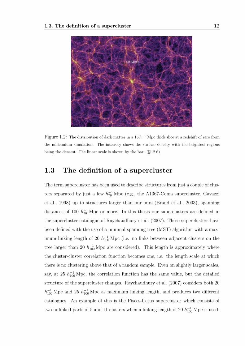
1.2.6 N-body simulations
As mentioned earlier when a region leaves the linear regime it is no longer possible
to analytically predict its evolution and hence numerical simulations are needed.
The Virgo consortium used the Millennium simulation of over 1010 particles to trace
the evolution of the matter distribution in a ΛCDM universe (Springel, 2005). The
model used a ΛCDM model with Ωdm = 0.205, Ωb = 0.045, ΩΛ = 0.75, h =
0.73 and an initial spectral index of n = 1. This has resulted in a sufficient mass
resolution over volumes similar to those of the large redshift surveys (2dFGRS,
SDSS) to allow direct comparisons with observations. The simulation volume was a
box of 500 h−1 Mpc which resulted in the 10 billion particles, each having a mass of
8.6×10⁸ h−1M⊙. This was enough for dwarf galaxies (L > 0.1L∗) to be represented
by approximately 100 particles, galaxies like the Milky way by approximately 1000
particles and rich clusters of galaxies several million particles.
1.3. The definition of a supercluster 12
Figure 1.2: The distribution of dark matter in a 15h−1 Mpc thick slice at a redshift of zero from
the millennium simulation. The intensity shows the surface density with the brightest regions
being the densest. The linear scale is shown by the bar. (§1.2.6)
1.3 The definition of a supercluster
The term supercluster has been used to describe structures from just a couple of clus-
ters separated by just a few h−170 Mpc (e.g., the A1367-Coma supercluster, Gavazzi
et al., 1998) up to structures larger than our ours (Brand et al., 2003), spanning
distances of 100 h−170 Mpc or more. In this thesis our superclusters are defined in
the supercluster catalogue of Raychaudhury et al. (2007). These superclusters have
been defined with the use of a minimal spanning tree (MST) algorithm with a max-
imum linking length of 20 h−1100 Mpc (i.e. no links between adjacent clusters on the
tree larger than 20 h−1100 Mpc are considered). This length is approximately where
the cluster-cluster correlation function becomes one, i.e. the length scale at which
there is no clustering above that of a random sample. Even on slightly larger scales,
say, at 25 h−1100 Mpc, the correlation function has the same value, but the detailed
structure of the supercluster changes. Raychaudhury et al. (2007) considers both 20
h−1100 Mpc and 25 h−1
100 Mpc as maximum linking length, and produces two different
catalogues. An example of this is the Pisces-Cetus supercluster which consists of
two unlinked parts of 5 and 11 clusters when a linking length of 20 h−1100 Mpc is used.

1.3. The definition of a supercluster 13
This however increases to one large supercluster of 19 members if the 25 h−1100 Mpc
links are used. The linking length of 25 h−1100 Mpc results in superclusters which have
a maximum size of the order 100 h−170 Mpc. It is therefore important to know at
which size superclusters become just a random collection of galaxies rather than a
statistically significant structure.
Pandey & Bharadwaj (2005) use SDSS data to find the maximum length of
filament which is statistically significant. They take a volume limited sample over
the redshift range 0.08 ≤ z ≤ 0.2, extinction corrected Petrosian r band apparent
magnitude 14.5 ≤ mr ≤ 17.5 and absolute magnitude range −22.6 ≤ Mr ≤ −21.6.
This results in 5315 galaxies distributed in two wedges, spanning 91 degrees (NGP)
and 65 degrees (SGP) in RA. and thickness 2 degrees.
They use a technique where the 2D galaxy distribution is embedded in a 1
h−1100 Mpc by 1 h−1
100 Mpc rectangular grid. Grid cells having a galaxy within them
are termed as filled (assigned a value of 1) and those without a galaxy present are
termed as empty (assigned a value of 0). The filamentarity of a cluster is defined
based on a single 2D “shapefinder” statistic (Bharadwaj et al., 2000), where a value
of 1 is a filament, a value of 0 is a square and the values change from 0 to 1 as
a square is deformed into a filament. They then use a statistical technique called
shuffle to determine the largest scale length at which the filamentarity is significant.
The shuffle technique involves taking squares with sides of length L. These
squares are then randomly interchanged, thus destroying structures larger than L
but maintaining those smaller than L. For a fixed value of L, if the shuffled data
has an average filamentarity lower than the initial data then the original data had
more filaments with length longer than L. They calculate the difference in the fil-
amentarity of the shuffled and original cluster data (χ2 per degree of freedom) at
each value of L. They find that shuffling the data with L>90 h−1100 Mpc does not
result in a significant difference in the filamentarity of the two samples. Therefore,
the longest filament which is statistically significant is 80 h−1100 Mpc, or 114 h−1
70 Mpc.
Therefore, our superclusters which have a maximum size of the order 100 h−170 Mpc,
should therefore be statistically significant.

1.4. Observational Surveys 14
1.4 Observational Surveys
1.4.1 The Two Degree Galaxy Redshift Survey
The Two degree Galaxy Redshift Survey (2dFGRS) is a large spectroscopic survey
in the southern celestial hemisphere covering approximately 1500 square degrees.
Spectra for 245,591 galaxies were obtained in three regions, the North Galactic pole
region , South Galactic pole region and a series of random fields. This makes it the
second largest redshift survey to date, coming above the VIRMOS galaxy redshift
survey (Le Fevre et al., 2004) of approximately 150000 galaxies but falling below the
Sloan Survey which is discussed later in this section. The survey is performed with
the Two-degree Field multifibre spectrograph on the Anglo-Australian telescope,
capable of observing up to 400 objects at once within the two degree field. The
survey is based on an extended version of the Automated Plate Measuring catalogue
of over 5 million objects.
The overall incompleteness of the source catalogue varying with apparent mag-
nitude is 10− 15%, the incompleteness being due to effects such as merged images,
misclassification of some galaxies as stars and the misclassification of some low sur-
face brightness galaxies as noise. The survey magnitude limit varies across the survey
regions and is detailed in the survey magnitude mask. Initially before improvements
to the photometric calibrations target galaxies were limited to extinction corrected
magnitudes of bJ > 19.45. The 2dFGRS is the first survey to be large enough to
study effects over scales of larger than 100 h−1 Mpc. One such effect that has been
studied is the Kaiser effect (Kaiser, 1987), which studies the gravitational collapse of
cosmological structures. In the collapsing regions there should exist coherent infall
velocities of galaxies which will cause an apparent flattening of structures along the
line of sight. Peacock et al. (2001) used the galaxy two-point correlation function
to show that the Kasier effect is observed for these large scales and combined with
CMB data their results are consistent with a Ωm = 0.3 universe. Other results have
included calculating the galaxy power spectrum (Percival et al., 2001), the luminos-
ity dependence of galaxy clustering (Norberg et al., 2001) and the environmental
effects on star formation rates near clusters (Lewis et al., 2002) to name just a few.

1.4. Observational Surveys 15
Figure 1.3: Map of the galaxy redshift distribution for the completed 2dFGRS survey. .Taken
from Colless et al. (2003). (§1.4.1)
1.4.2 The 2dFGRS Percolation-Inferred Galaxy Group cat-
alogue
The 2dFGRS Percolation-Inferred Galaxy Group (2PIGG) catalogue is a catalogue
of groups based on the North and South strips of the 2dFGRS catalogue consisting
of approximately 220,000 galaxies (Eke et al., 2004). They chose a friend-of-friends
algorithm to find the groups. These algorithms link together all the galaxies within
a certain linking distance of the centre of each galaxy. So that the groups all have a
similar overdensity throughout the sample, this linking length was varied with red-
shift to counter the reduced number density of galaxies detected at larger redshifts.
The linking length should ideally be scaled in the perpendicular direction (plane
of the sky) and the parallel (line of sight) directions such that a group sampled at
different completeness should have its edges in approximately the same position.
However, care has to be taken that the linking lengths do not become too large
compared to the size of gravitationally bound structures. The shape of the linking
volume was taken to be a cylinder to account for elongation in the redshift direction,
and to best recover groups that trace the underlying dark matter halo.
Eke et al. (2004) also showed that the overdensity enclosed in the group was
dependent on the mass of the underlying halo. This can result in a systematic

1.4. Observational Surveys 16
bias in the projected size and velocity dispersion, resulting in small groups with
overestimated sizes or large clusters with underestimated sizes. To correct for this
they estimated the halo mass in which each galaxy is found. This was done by
measuring the galaxy density relative to the background, and then using this density
contrast to scale the size and aspect ratio of the linking cylinder. The size of the
linking volume is thus dependent on the maximum size of the perpendicular linking
length (L⊥) , the aspect ratio of the linking cylinder (Rgal) and the number of mean
intergalaxy separations defining the perpendicular linking length (bgal). These values
are in physical coordinates and set at optimum values while the parameters in co-
moving space vary with redshift and galaxy density.
Optimum values were found by comparing groups found from a mock 2dFGRS
catalogue with their parent dark matter halos. The 220,000 galaxies in the initial
sample were reduced to 191,000 after all galaxies within fields with less than 70%
completeness, and in all sectors (overlapping field areas) with completeness less than
50%, were removed. Weights were then applied to these galaxies by assigning all the
galaxies in the parent APM catalogues with no recorded redshift to the nearest 10
members with redshifts. The co-moving number density of galaxies was calculated
at each angular position and redshift. This mean observed galaxy density for each
galaxy was then used with the friend-of-friends algorithm with optimum values of
L⊥ = 2 h−1 Mpc, Rgal = 11 and bgal = 0.13 to find real groups in the 190,000
galaxy sample. This resulted in 55 % of galaxies being part of groups of at least two
members. 28,877 groups were found with at least 2 members and 7,020 groups with
at least 4 members.
1.4.3 The Six degree Galaxy Survey
Since 2001 the Six degree Galaxy Survey (6dFGS) has obtained over 120,000 red-
shifts in the southern sky. The final release is due in late 2006, by which time the
survey will have covered an area 8 times larger than that of the 2dFGRS. The sur-
vey is performed with the six-degree field multi-object fibre spectroscopy system on
the UK Schmidt telescope at the Anglo-Australian Observatory (6dF). The 6dF is
capable of taking 150 simultaneous spectra in a field of a 5.7 degree diameter. The

1.4. Observational Surveys 17
primary sample for the survey is extracted from the near infrared (NIR) two micron
all sky survey (2MASS)(Jarrett et al., 2000). The use of a NIR survey means that
the bias towards currently star forming galaxies, found in the SDSS and 2dFGRS,
would be minimalised. Each field takes approximately 1.5 hours and repositioning of
fibres and other overheads take about 40 minutes, resulting in 5 fields being observed
a night on average.
1.4.4 The Sloan Digital Sky Survey
Funded by the Alfred P. Sloan Foundation, the Sloan Digital Sky Survey (SDSS) is
the largest redshift survey to date and is still growing. The fifth data release con-
tained spectra for approximately 675,000 galaxies and 79,000 quasars with the aim
being to get over 1 million galaxies by the end of the survey. Imaging is carried out
in drift scan mode using a wide-field 2.5 m telescope at Apache Point Observatory,
New Mexico. Photometry is gathered in five broad bands, (u,g,r,i,z) in the range
from 3000 to 10,000 A. Each plate can accommodate 640 fibres, about 50 of which
are reserved for calibration targets, which leaves approximately 590 fibres for tar-
gets. Plates are exposed in a series of 15 minute sessions after which signal-to-noise
ratio (S/N) diagnostics are performed. The 15 minute exposures are continued until
until the cumulative median (S/N)2 > 15 at g* = 20.2 and i* = 19.9 in each of
the 4 CCD detectors (One red and one blue in each of the two spectrographs). The
nominal exposure time is 45 minutes. The spectroscopic survey aims to observe a
complete sample of galaxies, selected to be brighter than r* = 17.77, using Petrosian
magnitudes 1. Like the 2dFGRS the SDSS has been used extensively to investigate
the large scale structure of the universe. Studies have included, the clustering prop-
erties of galaxy clusters (Basilakos & Plionis, 2004), constraining the amplitude of
the matter power spectrum (Viana, Nichol, & Liddle, 2002) and large scale galaxy
1Galaxies do not all have the same radial surface brightness profile, and have no sharp edges,
Therefore, a method is needed to measure a constant fraction of the total light, independent of
the position and distance of the object. The SDSS has adopted a modified form of the Petrosian
(1976) system, measuring galaxy fluxes within a circular aperture whose radius is defined by the
shape of the azimuthally averaged light profile.

1.5. Cosmology in this thesis 18
clustering (Gaztanaga, 2002), to name just a few.
1.4.5 Super COSMOS
SuperCOSMOS is a machine used to digitise Sky Survey plates taken with the UK
Schmidt telescope, the ESO Schmidt, and the Palomar Schmidt telescopes. The
photographic plates are digitised to 15 bits with a resolution of 10 microns. The
resulting database is approximately 2.5 terabytes in size and contains 3.7 billion
individual object detections. The database covers the southern sky (dec < +3.0)
in three wavebands (BRI), with the R band represented at two epochs. Initially the
source pairing was done “on-the-fly” but a more detailed analysis of merged objects
is performed in the SuperCOSMOS Science Archive (SSA). Each scanned plate in
the SSA results in a pixel map. This map is then processed using Image Analysis
Mode, or IAM, software to produce a list of parameterised detections on each plate.
The “on-the-fly” method uses a series of pair index pointers between any two given
plate datasets, however this can result in the same slave detection being paired with
more than one master image. The SSA uses the same pair indices but removes any
multiple pairings based on absolute proximity, i.e. the nearest slave is chosen.
1.5 Cosmology in this thesis
Throughout this thesis the cosmology used is ΩM = 1 and H0 =70 km s−1 Mpc−1,
though the trends we present do not crucially depend on these parameters. It can
be shown that for the Shapley supercluster, for example, a dark energy dominated
cosmology ΩΛ = 0.7, Ωm = 0.3, at the mean redshift of z = 0.0476 would be at a
distance of 211h−170 Mpc compared with 206 h−1
70 Mpc for our ΩM = 1 cosmology.
This amounts to a 2.5 % difference in the distances, which is within the error budget
of most of the calculations we perform.

1.6. Thesis Outline 19
1.6 Thesis Outline
In Chapter 2 we give a brief introduction into star formation in galaxies, covering
areas such as trends with time and environment, star formation indicators and a
summary of the 2dFGRS star formation parameter η. Chapter 3 investigates the
Pisces-Cetus, Horologium-Reticulum and Shapley superclusters, looking at their
spatial structure and obtaining estimates of their minimum mass and consequently
their mass overdensities. The star formation properties of the Pisces-Cetus super-
cluster are looked at in Chapter 4 using the η parameter. The dependency of star
formation on its environment is investigated in a range of areas including within
clusters and groups, within the supercluster and in the field, in dwarf and giant
galaxies and around low and high velocity dispersion clusters. Chapter 5 looks at
some of the same star formation environmental relations in much larger samples of
filaments of galaxies using the same η parameter. Star formation is also investi-
gated in Chapter 6, but this time 6dF equivalent widths are used to estimate star
formation within the Shapley supercluster region. Our findings are summarised in
Chapter 7 and future work discussed.

Chapter 2
Lady Astor: “Winston, if I were your wife I’d put poison in your coffee.”
Sir Winston Churchill: “Nancy, if I were your husband I’d drink it.”
Star formation in galaxies
2.1 Star formation as a function of time
It is generally accepted that the stellar populations in galaxies in the cores of clus-
ters are predominantly old. Most of the galaxies have early type morphology with
suppressed star formation, with the bulk of stars forming at z > 2. The tight cor-
relation of colour magnitude relations support this, as recent star formation would
result in a much greater scatter than that observed (Bower, Lucey, & Ellis, 1992;
Gladders et al., 1998). Other relations such as that between the Mg2 line strength
(metallicity indicator) and central velocity dispersion (e.g. Guzman et al., 1992) or
that in the fundamental plane of early type galaxies (e.g. Fritz & Ziegler, 2003) also
show little scatter.
With little star formation at the current epoch it is sensible to assume that as
you go back in time you will reach a period where the relations break down and
star formation is more prevalent. van Dokkum & Stanford (2003) have shown that
the fundamental plane relation remains tight at z = 1.27, but there is little or
no evidence for tight relations beyond z = 2. However, studying only the early
type galaxies or any subset of the total cluster population can result in biases. An
example of this is the “progenitor bias” described by van Dokkum & Franx (2001),
where by the progenitors of the youngest present day early type galaxies drop out
of the sample at high redshift. i.e. a significant fraction of present-day, early-type
20

2.1. Star formation as a function of time 21
galaxies was transformed from star-forming galaxies at z < 1 and so for z > 1,
galaxies which are early-type now may not be included in the sample.
The star formation rate (SFR) in cluster cores has also been studied as a function
of redshift. This has been extensively performed on the basis of colours. Butcher
& Oemler (1984) showed that clusters show a larger proportion of bluer (higher
temperature and higher SFR) galaxies at progressively higher redshifts. This ef-
fect has become known as the “Butcher-Oemler effect” and has been confirmed by
more recent studies (Margoniner et al., 2001). This has helped establish clusters as
evolving systems where star formation and galaxy morphology are dependent on the
environment. However, once again care has to be taken to consider possible biases.
The magnitude limit can be a potential bias where by blue galaxies will fade by up
to a magnitude when star formation ends and thus are not directly comparable to
the red galaxies. Another potential bias can come from the contamination of cluster
members by field galaxies due to projection effects. At low redshifts this effect may
be minimal, but at larger redshifts, with their bluer field populations, this effect will
be greater. De Propris et al. (2004) have concluded that the observed changes in the
blue fraction are dependent on the luminosity limit, cluster-centric radius and more
generally the local galaxy density but not the properties of the individual clusters.
Poggianti et al. (2006) also confirm the “Butcher-Oemler effect” but also show that
the morphology of galaxies change to later-type toward higher redshifts. Thus, there
is also a morphological version of the “Butcher-Oemler effect”.
The fraction of star forming galaxies as a function of redshift can also be studied
spectroscopically. Poggianti et al. (2006) use the Equivalent Width (EW) of the [OII]
line as an indicator of ongoing star formation in a high (z=0.4–0.8) and low (z=0.04–
0.08) redshift galaxy sample to find the fraction of passive galaxies. They propose a
scenario in which the passive galaxies consist of two populations, primordial which
had all their star formation at z > 2.5 and quenched galaxies where the SFR had
been reduced due to dense environments at later times. The Millennium simulation
is used to show that their observed relations between the fraction of passive galaxies
and velocity dispersion at high redshifts is consistent with that of galaxies that were
in groups at z = 2.5, with primarily a primordial passive population. The high

2.2. Star formation as a function of environment 22
redshift sample is found to be consistent with galaxies that have been in clusters
over the last 3 Gyr, with 60% quenched galaxies. This would mean that galaxy star
formation histories of galaxies are closely linked with the environment, even at high
redshift..
2.2 Star formation as a function of environment
Early works have also shown that the relative morphological content of galaxies in
a given volume of space is dependent on the local projected galaxy density, with
more elliptical galaxies and less spirals at higher densities (e.g. Dressler, 1980).
Menanteau et al. (2006) have shown that the SFR is dependent on the morphology of
the galaxy with spiral galaxies being the main provider to the star formation density
at all redshifts. However, Ravindranath et al. (2006) use high redshift Lyman-break
galaxies 2.5 < z < 5 to show that at higher redshifts many star forming galaxies
have elongated structures. Thus at higher redshifts a significant fraction of star
formation may be occurring in galaxies which are comprised of gas rich filaments.
Therefore, morphological type can not always be used as a proxy for SFR.
The effect of the density of the environment has been studied extensively in
clusters of galaxies, where a large range of projected surface density can be probed.
There is clear evidence that SFRs are highly suppressed in galaxies within the cores
of rich clusters (Dressler, 1980). Furthermore, the current SFR is shown to increase
with decreasing density and increasing distance from a cluster core. Balogh et al.
(1999) were one of the first to study the SFR away from cluster cores. They found
a strong radial dependence on SFR and that the SFR had not yet reached the field
value as far out as the virial radius. The arrival of the 2dFGRS and SDSS has
allowed much more accurate work to be done with the detailed redshift information
removing contamination from interlopers. From these surveys, Lewis et al. (2002)
and Gomez et al. (2003) have shown a correlation between the median SFR and
the local density. There is a sharp transition in the correlation at approximately 1
galaxy per h−2 Mpc−2. Beyond 1 galaxy per h−2 Mpc−2 the median SFR has values
very similar to the field values but below 1 galaxy per h−2 Mpc−2 the median SFR
2.3. Star formation indicators 23
begins to drop rapidly.
The SFR in clusters away from the core does not reach that of the field until
beyond 3 h−1Mpc (∼2 times the virial radius) from the centre of the clusters. This
shows that ram pressure stripping can’t be the only process that is suppressing the
SFR as this is only present in the most dense environments. They also conclude
that the SFR dependence on density is independent of the velocity dispersion of
the cluster and hence the SFR is independent of the large scale structure of the
environment (group or cluster). However, while Balogh et al. (2004) also find that
the correlation is independent of velocity dispersion, they suggest that fewer galaxies
in supercluster like environments have significant Hα emission and that there may
be some correlation at lower densities on scales > 5 h−1 Mpc.
Haines et al. (2006a) compare the environmental dependence of giant (MR <
−20) and dwarf galaxies. They find that the SFR in giant galaxies are in agreement
with the above studies with SFR approaching field values at 3–4 virial radii. How-
ever, the dwarf galaxies show a sharp transition at approximately the virial radius
from predominantly passive to predominantly star forming. This means that dwarf
galaxies may preferentially lose their gas reserves and hence become passive when
they encounter effects such as ram pressure striping or galaxy harassment.
2.3 Star formation indicators
2.3.1 Recombination lines of Hydrogen
High temperature OB stars cause the ionisation of the HII nebular gas that sur-
rounds them. The hydrogen electrons ionised by Lyman continuum photons with
energies above 13.6 eV, recombine with the atoms. The initially excited atom jumps
down to less excited states, and, in doing so, releases energy at specific wavelengths,
which is seen as emission lines in the spectrum. For a radiation bounded system, the
flux of the hydrogen recombination lines scales directly with the flux of the ionising
radiation from the stars. The strongest emission line is the Lyman Hα , the strength
of which can be determined by taking the equivalent width. Equivalent Width is
defined as the rectangular section of a surface counted between the level of the con-

2.3. Star formation indicators 24
tinuum, normalised to unity, and reference zero, having a surface area identical to
the profile of the line. The relation of Kennicutt (1998b),
SFR(IR) (M⊙yr−1) = 7.9 × 10−42LHα (erg s−1), (2.1)
where LHα is the total Hα luminosity, can be used to gain an estimate the SFR.
Because nearly half of the ionising atoms produce a Hα photon (Kennicutt et
al., 1998a) this technique is very sensitive. This combined with the direct coupling
between nebular emission and SFR and the ability of even small telescopes to obtain
high resolutions has enabled this technique to provide the most detailed information
on SFRs in galaxies.
However, the observed spectrum of the galaxy is a combination of the nebular
emission lines and the combined spectra of the constituent stellar population. There-
fore, the accurate measurement of the nebular emission lines relies on the removal of
the absorption lines in the underlying stellar spectrum. The stellar spectrum can be
recreated by either spectral synthesis or evolutionary synthesis models (e.g., Bruzual
& Charlot, 2003). Spectral synthesis creates the model spectrum by integrating the
spectra of star clusters spanning the range of types of star expected to be present
in the galaxy population. This is best used in elliptical galaxies and spiral bulges
where the population types are well constrained. In active star forming galaxies the
evolutionary synthesis is best used. These use a theoretical stellar evolution model,
coupled with models of stellar atmospheres and an assumed initial mass function to
create integrated spectra over a range of star formation histories. These are then
compared with the observed spectrum to find the stellar properties of the galaxy.
Extinction due to dust in the interstellar medium remains the main problem
with this technique. The extinction in normal galaxies can be estimated from the
reddening of [HII] regions or comparing the integrated Hα and thermal radio fluxes
(e.g., Ruffle et al., 2004). The nuclear regions of galaxies and the starburst regions
found in many mergers, can have much higher extinctions than those calculated for
normal galaxies. The emission line flux only traces the most massive stars requiring
the extrapolation of the Initial Mass Function (IMF) to lower stellar masses. The

2.3. Star formation indicators 25
[NII] doublet (6548 A and 6584 A) are very close to the Hα emission line and are
sometimes blended together. When separated high [NII]/Hα ratios can suggest
photo-ionisation due to the presence of an Active Galactic Nucleus (AGN) (Veilleux
et al., 1994).
While the Hα emission line is the strongest and hence most commonly used, any
hydrogen recombination line can be used, Brγ and Brα hydrogen emission lines in
Infrared wavelengths are often used for dusty regions. At higher redshifts the Hα
emission lines become unobservable in optical spectra (z & 0.4) and the higher order
Balmer lines such as Hβ or the [OII] doublet are substituted.
Using the Hβ emission line has essentially the same strengths and weaknesses
as the use of the Hα line. It too is sensitive only to the most massive stars and
suffers from the same dependence on dust extinction. In fact, Hβ encounters more
interstellar dust attenuation and is slightly more sensitive to the underlying stellar
absorption. Kennicutt (1992) regards its use as limited in normal galaxies, due to the
difficulty in accounting for the underlying stellar absorption, although population
synthesis models can try to account for this (Tremonti et al., 2004). There is a
strong correlation between the equivalent widths of Hβ and Hα+[NII] (Kennicutt,
1992). [OIII] has been used as a crude estimator of SFR but shows such a large
dispersion in relations to Hα that it has little significance (Kennicutt, 1992).
2.3.2 Ultraviolet continuum emission from hot stars
Young stars (< 107 yr) contribute most of the Ultraviolet (UV) flux in a galaxy,
hence the UV continuum in the range 1300-2500A is an indicator of the galaxies
SFR. This method allows the tracing of stars that are not hot or massive enough
to produce [HII] regions. The SFR in this way can be found using the relation of
Kennicutt (1998b),
SFR(UV) (M⊙yr−1) = 1.4 × 10⁻²⁸Lν (erg s−1Hz−1), (2.2)
where Lν is the total luminosity per frequency interval.
While this method is undoubtedly a useful indicator it has several drawbacks.

2.3. Star formation indicators 26
The most serious of these is that the UV flux is very sensitive to interstellar extinc-
tion, meaning that the UV spectrum is of little use in the dusty starburst regions
of galaxies. The wavelength band used is also visible from the ground only for high
redshift systems.
2.3.3 Infrared thermal emission
Infrared (IR) emission in the 8–1000 µm band in star forming galaxies can arise
from three different processes, (a) emission from dust heated by young OB stars,
(b) emission from the photospheres of evolved stars as they lose mass, and (c) from
dust distributed throughout the interstellar medium, which is heated by the general
stellar radiation. The absorption cross section of the dust is highly peaked in the
UV and the absorbed radiation is re-emitted in the IR. If it is assumed that young
stars dominate the radiation field in the UV and visible bands, then the last two of
these processes are negligible. It is then also assumed that the opacity of the dust
in a galaxy is infinite, then the IR SFR is a good representation of the actual galaxy
SFR. The relation of Kennicutt (1998b),
SFR(IR) (M⊙yr−1) = 4.5 × 10−44LIR (erg s−1), (2.3)
where LIR is the total Ir luminosity in the 8-1000µ m band, can be used to gain the
IR SFR.
Calibration of the SFR for normal galaxies is not an easy task. The dust grains
absorb radiation with a broad range in wavelengths and hence radiation from young
and old stars. Conclusively separating the star forming component has proven elu-
sive. However, in the case of dusty starburst regions, the young stars dominate,
and the optical depth of the dust is so high that the IR emission is effectively the
bolometric luminosity of the starburst.

2.4. Star formation in interacting galaxies 27
2.3.4 X-ray Luminosity
It has been shown (e.g., Grimm, Gilfanov, & Sunyaev, 2003; Gilfanov, Grimm, &
Sunyaev, 2004) that high-mass X-ray binaries (HMXB) can be used as SFR indi-
cators. The X-ray luminosity (Lx) distribution of HMXBs can approximately be
described by a luminosity function which is a power law with a slope of ∼ 1.6 and
a cut off at log(Lx) ∼ 40.5, the normalisation of which is proportional to the SFR.
The 2-10 KeV Lx of a normal galaxy with sufficiently high SFR/M∗ ratio, where M∗
is the total stellar mass, is dominated by the emission from HMXBs. Therefore, Lx
can be used as a SFR indicator for normal galaxies. The Lx–SFR relation is only
linear for higher SFRs, the break in the relation occurring at SFR ∼ 4.5 M⊙ yr−1
or Lx ∼ 3 × 1040 erg s−1. In the linear regime the SFR of stars with M > 5 M⊙ is
given by,
SFR(Lx) (M⊙yr−1) =L2−10KeV
6.7 × 1039 (erg s−1), (2.4)
where L2−10KeV is the X-ray luminosity in the range 2-10 KeV. However, contamina-
tion of the SFR from the emission of the central supermassive black holes in which
even low luminosity AGNs can outshine the X-ray binaries and the contribution
of low-mass X-ray binaries which are unrelated to SFR and may be important for
low SFR can be a problem. The latter has been suggested by Gilfanov, Grimm, &
Sunyaev (2004) to be responsible for Ranalli, Comastri, & Setti (2003) obtaining a
linear Lx–SFR relation for all SFRs.
2.4 Star formation in interacting galaxies
2.4.1 Star formation mechanisms
The diversity of the star forming environments in interacting galaxies suggests that
several physical processes are responsible for the increased SFR seen in starburst
galaxies. Potential mechanisms for causing varying levels of increased SFR in dif-
ferent environments are discussed below.

2.4. Star formation in interacting galaxies 28
Gravitational star formation thresholds
Nonlinear star formation features are seen in a wide range of interacting and normal
galaxies. An abrupt transition is seen in most late-type spirals where at a certain
radius SFR drops to very low values. Thresholds are also seen in gas-rich S0 galaxies
and low surface brightness galaxies. Kennicutt (1989) proposed that these thresholds
could be associated with large scale gravitational thresholds for the growth of density
perturbations. The Toomre parameter (Q) is the ratio of the critical density for star
formation at a given radius to the actual gas density. Regions that have Q ≫ 1
have suppressed star formation while regions with Q ≪ 1 would have unimpeded
star formation. However, regions with Q ∼ 1 would be stable but easily perturbed.
When galaxies interact, local compressions in density waves could cause the gas in
these stable regions to exceed the critical threshold, leading to an increase in SFR.
Cloud collisions
The variation in star formation thresholds can only account for a variation in SFR by
∼ 5%, which is not high enough to explain the large increases in strongly interacting
systems. When two galaxies closely interact, clouds of gas from the two galaxies
may collide with each other. Collision velocities may be high enough to cause
shocks, which can compress clouds inducing small-scale gravitational collapse and
star formation (e.g., Olson & Kwan, 1990). If the galaxies do not touch, but still
interact, small perturbations could cause gas clouds with orbits close to one another
to collide and start star formation (e.g., Lin, Pringle, & Rees, 1988). The rate of
collisions depends on the ratio between the lifetime of a cloud and the time interval
of the collision (Struck-Marcell & Scalo, 1987).
Tidally induced bars
One of the most critical pre-requisites for the most active starbursts is the transport
of large masses of interstellar gas at the centre of the merger. If one of two tidally
interacting systems has a large solid-body like rotation curve, then its partner can
induce a bar which out-lives the interaction itself. This can channel gas into the
nuclear region perhaps leading to a nuclear starburst (Noguchi, 1988). The gas and

2.4. Star formation in interacting galaxies 29
star formation is often found in nuclear rings of dense young star clusters known as
“hotspots” or twin “peaks” (Kenney, 1994) often surrounding an AGN. This process
is unlikely to produce very luminous starbursts but may be important in the lower
level nuclear activities of many interacting galaxies.
2.4.2 Environmental influences
The environment of a galaxy is an essential ingredient of its evolution and SFR
properties. The relations between the density of galaxies, the presence of an intra
cluster medium (ICM), gas reserves, temperature and the velocity of encounters in-
fluence the resulting SFR, either enhancing or suppressing the rate. Many studies
of Hα and IR have shown increased SFR in merging and interacting galaxies (e.g.,
Bushouse, 1987; Kennicutt et al., 1987; Xu & Sulentic, 1991; Liu & Kennicutt, 1995).
On average the equivalent widths of the interacting galaxies show an enhancement
in SFR of approximately double that of an isolated sample. The majority of in-
teractions show only modest enhancements. However, they range from practically
no SFR enhancements to systems where a significant fraction of their total stellar
mass is star forming. Some of the main interacting processes which may influence
the onset of the above mechanisms are described below.
Galaxy Harassment
One of the most important influences on induced SFRs in galaxy-galaxy interac-
tions is tidal in nature, where the gravitational attraction of galaxies influence each
other. Multiple close encounters between galaxies at high speeds can deform gas
clouds and/or cause them to collide leading to an increased SFR. Moore et al. (1996)
used high resolution numerical simulations to study the effect of these multiple en-
counters and termed the phrase “galaxy harassment”. They conclude that “galaxy
harassment has the potential to change any internal property of a galaxy within a
cluster, including the gas distribution and content, the orbital distribution of stars
and the overall shape”. From these early results galaxy harassement has been inves-
tigated in numerous papers and used to explain the morphological transformation
of galaxies in clusters, in particular the formation of dwarf ellipticals, and even as

2.4. Star formation in interacting galaxies 30
a source of fuel for quasars (e.g., Lake & Moore, 1999; Matkovic & Guzman, 2003;
Davies, Roberts, & Sabatini, 2005; Haines et al., 2006b). Observationally galaxy
harassment can be seen on galaxies with long tidal tails, drawn out by the close
encounters and rings around a stellar bar.
Tidal influence of a cluster potential
Galaxies falling into a cluster potential will experience a strong differential force the
strength of which depends on the galaxies orbit. The tidal force experienced is of
the order of,
Ftide ∼GM(r)
r3∼ σ2
cl
r2, (2.5)
where σcl is the cluster velocity dispersion, r is the distance from the cluster centre,
M(r) is the enclosed mass within radius r and G is the gravitational constant. The
tidal forces of the cluster potential can cause density waves in the gas of the infalling
galaxies leading to enhanced star formation where the densities become high enough.
Strangulation
It has been shown that galaxies can be surrounded by a halo of hot gas with a
temperature of up to a few million degrees Kelvin (e.g., Pedersen et al., 2006).
However, warm halos of gas with a temperature of a few hundred thousand degrees
Kelvin, which is too cool to be seen in X-ray detections and too warm to be seen
in radio detections, may be present around most galaxies. This halo of warm gas
would provide a reserve of gas which can be used to fuel star formation in the future.
As a galaxy falls into a cluster potential well, tidal effects can strip this reserve of
gas from the halo. This will result in a “strangulation” (e.g. Larson, Tinsley, &
Caldwell, 1980) of star formation, where star formation in the disk continues until
gas in the disk of the galaxy is used up, with no reserve of gas to fuel further star
formation. More massive galaxies will be more able to retain their warm gas haloes.

2.4. Star formation in interacting galaxies 31
Ram pressure stripping
As a galaxy falls in towards the centre of a cluster it will encounter the ICM. The
ICM is hot gas which has been ejected from galaxies by early supernovae-driven
winds. In the centres of clusters the density of the ICM is high enough that the
galaxies moving through it will experience a strong drag force known as ram pressure.
Ram pressure can strip the gas from the disk of a galaxy causing the suppression
of star formation at the current time. Gunn & Gott (1972) give the conditions for
ram pressure stripping to be if the force due to ram pressure exceeds the restoring
gravitational force, given by,
Pram ≥ 2πGσstarσgas, (2.6)
and,
Pram = ρicmV 2gal, (2.7)
where Pram is the ram pressure, G is the gravitational constant, σstar is the stellar
surface density, σgas is the surface density of the gas, Vgal is the velocity of the galaxy
and ρicm is the density of the ICM.
Mergers
Evidence for the merging of galaxies in clusters has been demonstrated optically and
with X-ray data (e.g. Mahdavi et al., 1996; Mohr, Geller, & Wegner, 1996). This
is consistent with the hierarchical growth of structure with highly evolved galaxies
being found in clusters which are not yet in equilibrium. The process of merging can
cause bursts of star formation through effects such as cloud collisions. Larger galax-
ies have a greater merger cross section and hence mergers between dwarf galaxies
will be rare. Gnedin (2003) show that the number of close encounters experienced
by a galaxy can be given as,
Nenc ≈Ng
4π3
R3cl
πR2g
√2σcltH , (2.8)
2.4. Star formation in interacting galaxies 32
where σcl is the cluster velocity dispersion, Rcl is the cluster virial radius, Ng is the
number of galaxies in the cluster and tH is the Hubble time. The probability of a
merger is then given by,
Pmer ∼ Nenc
(
σg
σcl
)4
, (2.9)
where σg is the galactic velocity dispersion.
Evaporation
As the cool gas in a galaxy encounters the hot ICM the galaxy can lose the gas
through evaporation. Fujita & Goto (2004b) show the time scale of the evaporation
of the cool gas can be given as,
te ≈3kbTicmMcold
2µmH |L|, (2.10)
where kb is the Boltzman constant, Ticm is the temperature of the ICM, µ(= 0.6) is
the mean molecular weight, mH is the Hydrogen mass, Mcold is the mass of cold gas
in the galaxy and L is the energy flux from the hot ICM surrounding the galaxy via
thermal conduction. The loss of the cool gas will curtail the ability of the galaxy to
form stars.
Active galactic nuclei
The process of interaction between galaxies can also trigger non-thermal nuclear
activities, creating active galactic nuclei (AGN). These AGN and the nuclear star-
bursts are closely intertwined and occur together in many interacting and normal
galaxies. However, it has been shown that galaxies dominated by nuclear star for-
mation are more prevalent in interacting systems (Sekiguchi & Wolstencroft, 1993),
and galaxies with AGN or composites may be as low as 15% (Brinchmann et al.,
2004) overall.

2.5. A star formation index from 2dFGRS spectra: the η parameter 33
2.5 A star formation index from 2dFGRS spectra:
the η parameter
The flux calibration of the 2dF spectra is unreliable due to instrumental limita-
tions. The calibration of fibre spectra is difficult to achieve due to, (a) astromet-
ric/positioning errors, which combined with the small fibre aperture prevent re-
producible sampling of each galaxy’s light distribution, (b) chromatic variations in
distortion, and (c) residual errors in the atmospheric dispersion correction (see Col-
less et al., 2001). Consequently a comprehensive study of the shape of the spectral
continuum is not possible. In order to find a parameter sensitive to SFR that can be
extracted from the uncalibrated 2dFGRS spectra, a Principal Component Analysis
of the galaxy spectra is the best method of gaining spectroscopic data . This essen-
tially measures the strength of the emission and absorption lines while remaining
insensitive to the continuum.
2.5.1 The Principal Component Analysis
Madgwick et al. (2002) initially took all the 2dFGRS observations until January
2001. This comprised a total of 111,404 galaxy spectra in the northern region and
60,062 in the southern region. They removed those galaxies which did not have an
accurate redshift (Q < 3, which is those galaxies which have a redshift which is,
probable, reliable, or reliable with a high quality redshift (see Colless et al., 2001))
, repeated observations and spectra with a signal to noise ratio of less than or equal
to 10. With a redshift cut of z≤ 0.15 to avoid corruption due to sky emission and
atmospheric absorption this left a total sample of 75,589 galaxies.
From this sample they defined a new parameter η based upon a Principal Com-
ponent Analysis (PCA) of the galaxy spectra. PCA is a statistical technique which
is used to reduce the dimensionality of the data to summarise the parts that are
useful to the user. In this case it does this by identifying the components of the
spectra that best discriminate between the galaxies. A detailed description of the
technique can be found in Glazebrook, Offer, & Deeley (1998).
The significance of each successive principal component was found to drop off

2.5. A star formation index from 2dFGRS spectra: the η parameter 34
so sharply that the first two components retained two-thirds of the total variance
within the population. Thus from the initial 738 channels needed to describe each
spectrum, now only 2 were needed. The principal components were determined from
a subsample of the main sample, and these used to find the projections of the rest
of the sample. The subsample was chosen to have an absolute magnitude limit of
–18.0 corresponding to a redshift of approximately 0.1. This makes the process less
prone to bias from relationships between the luminosity and type of galaxy.
It was found that the first eigenspectrum derived from the PCA contains approx-
imately an equal contribution from both the continuum and the emission/absorption
lines. However, the second eigenspectrum is dominated by the emission and absorp-
tion lines. Therefore by taking linear combinations of the two, the line features can
be maximised, see Fig. 2.1. By maximising the emission and absorption features
they were in effect high-pass filtering the spectra. This meant that the projec-
tion was relatively stable to uncertainties in continuum measurements. Therefore,
once the projection was chosen, the η parameter was defined as: η = apc1 − pc2.
Where pc1 and pc2 are the first and second projections onto the principal axes and
a is a constant which maximises the absorption and emission features. Identifying
the most stable projection in the pc1, pc2 plane between repeated pairs of spectral
observations gave a value of a = 0.5 ± 0.1.
By comparing the values from approximately 2000 repeat observations an es-
timate of the uncertainties in the PCA was obtained. The difference in the two
projections between repeat observations had 1σ dispersions of 2.9 and 1.7 for pc1
and pc2 respectively. However the combination of the two in the η parameter is
greatly reduced having a 1σ dispersion of 0.7.
The analysis has been expanded to now contain 192,982 galaxies with an η value
from a total of 245,591 galaxies in the final catalogue.
2.5.2 Relationships with other parameters
Madgwick et al. (2002) plotted the relation between the η parameter and its mor-
phological type for the spectrophotometric standard galaxies in Kennicutt’s atlas
(Kennicutt, 1992). It can be seen in Fig. 2.2 that there is a relation between the

2.5. A star formation index from 2dFGRS spectra: the η parameter 35
Figure 2.1: The first two principal components identified from the 2dF galaxy spectra and the
linear combinations which isolate either (a) the continuum slope or (b) the line features (Madgwick
et al., 2002). (§2.5.1)
morphological type and the value of η. Thus our own galaxy, the Milky way (Sb),
would have a η of between approximately 0 and 2. It is also possible to see that
a histogram of the η parameter is bimodal. The first peak corresponds to mainly
E/S0 galaxies, which would be consistent with little or no star formation at the
current time at these low η values. Approximately 40% of the galaxies are in the
first passive galaxy peak.
Madgwick et al. (2003) compared the value of η derived for each galaxy to the
equivalent width of the Hα emission-line spectra. It can be seen in Fig. 2.3 that
with some scatter there is a strong linear correlation between the two quantities.
A Hα EW of 0.0 corresponds to η ≈ −2.0 and A Hα EW of 50.0 corresponds to
η ≈ 7.0.
Madgwick et al. (2003) also compare the η with the birth rate parameter, b,
which is the ratio of the current SFR to the past averaged SFRs. They initially
derive b using a simple model of the star formation history in terms of an exponen-
tial function of time (Bruzual, 1983) with a Kennicutt (1983) initial mass function of:

2.5. A star formation index from 2dFGRS spectra: the η parameter 36
Figure 2.2: (Top) The distribution of η projections for the volume-limited sample of 2dF galax-
ies.Vertical lines show the devisions in η that correspond roughly to E/S0, early type S, late type
S and Irr, used in the analysis of Madgwick et al. (2002) (Bottom) The η projections calculated for
a subset of the Kennicutt Atlas galaxies. This plot is taken from Madgwick et al. (2003). (§2.5.2)
Figure 2.3: The correlation between η and the equivalent width of the Hα emission line for a
sample of high signal-to-noise ratio emission-line spectra (Madgwick et al., 2003). (§2.5.2)

2.5. A star formation index from 2dFGRS spectra: the η parameter 37
SFR(t) =1
τe−(t−tf )/τ , (2.11)
where tf is the time at which star formation first commences and τ is the charac-
teristic timescale of the star formation.
The PEGASE software package is used to realize the model and deals with other
tasks such as determining the strengths of nebula emission lines and dust extinction.
Spectral histories of a given galaxy are compiled for a range of formation times (0–20
Gyr) and lengths of star formation activity (0–2 Gyr). The value of b is determined
from:
SFR(t)
〈SFR(t)〉past=
(t − tf)
τ
e−(t−tf )/τ
(1 − e−(t−tf )/τ )= b. (2.12)
The same analysis is also performed using a semi-analytic model. In the hier-
archical model for the universe galaxies have built up from mergers and accretion.
Mergers can trigger bursts of star formation, which in turn may inhibit future forma-
tion by expelling gas from the galaxy on stellar winds. This model can be convolved
with stellar population models to produce model spectra. Madgwick et al. (2003)
use a multi-metalicity GISSEL model (Bruzual, 1983) and a Salpeter IMF. They
construct a mock 2dF catalogue of 2,611 model galaxies with the same magnitude
limit, wavelength coverage, spectral resolution and redshift range as the actual 2dF-
GRS. They derive the principal components of the mock catalogue and the birth
rate parameter b for each galaxy. They show that b has a strong relationship to the
η parameter in both the simple model and the semi-analytic model. This relation is
shown for the semi-analytic model in Fig. 2.4. It can be seen that galaxies with an
η of less than approximately –1.4 have a value of b < 0.1, where the current SFR is
only 10% of what it was in the past.

2.5. A star formation index from 2dFGRS spectra: the η parameter 38
Figure 2.4: (Left) η plotted versus b for each galaxy in the SAM mock-galaxy catalogue. (Right)
The mean value of η versus b for these galaxies (the dashed lines show the 1 σ uncertainties). Also
shown on this plot (dotted lines) are the cuts in η used in Madgwick et al. (2002) to calculate
the 2dFGRS luminosity functions per spectral type. It can be seen, for example, that the Type I
galaxies of that paper (η < −1.4) correspond to galaxies with b < 0.1, or, alternatively, galaxies
with current star formation activity that is only 10 per cent of their past-averaged rate. Figure
taken from Madgwick et al. (2003). (§2.5.2)
2.5.3 Separating the star-forming and non star-forming pop-
ulations
As mentioned previously (also see Fig. 2.5) a histogram of the η parameter is ex-
tremely bimodal. The first narrow peak corresponding to the non star-forming
galaxies (approximately 30 % of all z < 0.1 galaxies) and the wider second peak the
galaxies with current star formation.
To obtain the probability that a given galaxy falls within the first or second
peak, P (η), a series of likely functions were fitted to the two peaks such that,
P(η) = αg(η) + (1 − α) f(η), (2.13)
where f(η) is a function of η to fit the first peak, g(η) is a function of η to fit the
second peak and α is a constant. P (η) can be maximised such that,

2.5. A star formation index from 2dFGRS spectra: the η parameter 39
Figure 2.5: A histogram of the η parameter for all 2dFGRS galaxies with z < 0.1 binned in 0.1
η bins. (§2.5.3)
L =∑
lnP (η). (2.14)
The first peak was fitted with a standard Gaussian function such that,
f(η) =1
σ√
2πe
−(η−µ)2
2σ2 , (2.15)
where µ is the position of highest point of the peak and σ is the standard deviation
of the peak.
The second peak was fitted with an extreme value distribution such that,
g(η) =e(σ−η)/µ−e(σ−η)/µ
µ. (2.16)
L was fitted using the NAG routine E04JYF and the resulting fit can be seen as
the dashed line in Fig. 2.6. However, it can be seen in Fig. 2.7 when the values of µ
and σ obtained are used to plot the individual functions the Gaussian seen as the
dashed red line is not an appropriate fit to the first peak.

2.5. A star formation index from 2dFGRS spectra: the η parameter 40
Figure 2.6: Composite fit to the 2dFGRS η parameter distribution. The resulting fit shown
as the dashed orange line is a combination (eq.Fig. 2.13) of a Gaussian and an extreme value
distribution. The histogram shown is for the entire 2dFGRS binned in 0.1η bins. (§2.5.3)
Figure 2.7: Individual fits to the 2dFGRS η parameter distribution. The red dashed line is the
Gaussian function and the dashed blue line the extreme value distribution plotted with the values
of µ and σ obtained from the composite fit. The histogram shown is for the entire 2dFGRS binned
in 0.1η bins. (§2.5.3)

2.5. A star formation index from 2dFGRS spectra: the η parameter 41
The above fitting of a sum of two distributions did not lead to a more elegant
separation of the star-forming and non star-forming populations. A KMM algorithm
(Ashman, Bird, & Zepf, 1994) could also have been used to partition the data in two
subpopulations. However in the end it was decided that a complex solution to the
bimodality was not needed and a transitional value set at η = −1.4, below which all
galaxies will be classified as “passive” was chosen. This corresponds to, the divide
between E/S0 and Sa galaxies in Fig. 2.2, a Hα EW∼ 3 in Fig. 2.3 and a b < 0.1 in
Fig. 2.4, where the current SFR is only 10% that it was in the past.

Chapter 3
Viscount Horatio Nelson: “Thank God I have done my duty.”
Supercluster structure
Superclusters are an essential tool to study the largest-scale density perturbations
that have given rise to structure in the Universe (e.g., Bahcall, 2000). These are
particularly interesting since they have always evolved in the linear regime and can
be analytically tractable. Superclusters can be useful in quantifying the the high-end
mass function of collapsing systems and ratio of mass to light on the largest scales,
thus being useful in discriminating between dark matter and structure formation
models (e.g., Kolokotronis, Basilakos, & Plionis, 2002; Bahcall, 1988).
3.1 Minimal spanning tree supercluster structure
Superclusters are expected to be predominantly filamentary structures. Numer-
ical simulations of the evolution of large-scale structure (e.g., Bond, Kofman, &
Pogosyan, 1996; Colberg, Krughoff, & Connolly, 2005), as well as the analysis of
large-volume surveys like the 2dFGRS (e.g., Pimbblet, Drinkwater, & Hawkrigg,
2004) or studies of individual systems of superclusters (e.g., Bagchi et al., 2002;
Ebeling, Barrett, & Donovan, 2004) show the pre-eminence of filamentary struc-
tures. Nevertheless, supercluster catalogues are usually constructed (e.g., Einasto
et al., 1994; Zucca et al., 1993) using percolation or friends-of-friends algorithms
which do not take this geometrical feature into consideration.
Recently, Raychaudhury et al. (2007) have compiled a catalogue of supercluster-
size structures from a redshift survey of Abell clusters (z < 0.1) using the minimal
42

3.1. Minimal spanning tree supercluster structure 43
spanning tree statistic, which contains all the information used in a percolation anal-
ysis (Bhavsar & Splinter, 1996), and is particularly sensitive to filaments (Bhavsar
& Raychaudhury, 2000).
In this Chapter we investigate the structure of the three richest superclusters in
the catalogue of Raychaudhury et al. (2007), Horologium-Reticulum, Shapley and
Pisces-Cetus. We also gain estimates of the mass overdensity within each of the
superclusters.
3.1.1 The Pisces-Cetus supercluster
More than a decade ago, in a series of papers, Tully (1986, 1987, 1988) pointed
out the Pisces-Cetus supercluster to be one of the five richest systems of clusters
of galaxies in the z < 0.1 Universe, and speculated that it could be as large as
300 h−170 Mpc across, and might include the Local Group. Subsequent work (e.g.,
Zucca et al., 1993; Einasto et al., 1994) has pointed out interesting features of
significantly smaller substructures of this remarkable web of galaxies, groups and
clusters, and at least one unusually large void (Burns et al., 1988).
The Pisces-Cetus supercluster is found to straddle the 2dF galaxy redshift survey
(Colless et al., 2003) [2dFGRS] and the Sloan Digital Sky Survey (Abazajian et al.,
2005) [SDSS] regions.
In the supercluster catalogue of Raychaudhury et al. (2007), the Pisces-Cetus
supercluster occupies a region of about 700 sq. deg. of the (equatorial) southern
sky. While using the Minimal Spanning Tree (MST) in constructing this catalogue,
if a maximum edge-length of 20 h−1100 Mpc is used, the system breaks up into two
filaments (A, B) of 11 and 5 clusters respectively, at mean redshifts of 0.0625 and
0.0545 respectively. If, however, adjacent clusters on the tree are allowed to be
separated by a distance of up to 25 h−1100 Mpc, the supercluster becomes a long
filament of 19 clusters at a mean redshift of 0.0591, making the supercluster the
third richest in the catalogue (following the Shapley and Horologium-Reticulum
superclusters). This is illustrated in Fig. 3.1, where the clusters excluded by the
former consideration are shown to be connected to the main tree by dashed lines.
The clusters comprising the Pisces-Cetus supercluster from the MST analysis of

3.1. Minimal spanning tree supercluster structure 44
Raychaudhury et al. (2007) form the core of our sample, and are listed in Table 3.1.
Unlike MST analyses of galaxy catalogues, where completeness is an important con-
sideration, the supercluster list obtained in this catalogue is considered reasonably
complete since it arises from an analysis of rich Abell clusters in the volume closer
than z < 0.1 (Galactic latitude |b| > 20).
To the member list of the Pisces-Cetus Supercluster from the above list, we
added a few clusters, in the same volume as the filament, from the Supplementary
Abell cluster catalogue (Abell et al., 1989) and the Edinburgh-Durham Southern
Galaxy Cluster Catalogue (Lumsden et al., 1997). These extra clusters were taken
as potential members of the supercluster if their redshift as derived in §3 was found
to be consistent with the other members.
A plot of these clusters within the supercluster region and redshift range, in-
cluding the connecting MST, can be seen in Fig. 3.1. Also plotted are the groups
of galaxies in the region of the supercluster covered by the 2dFGRS (δ < −25 )
from the 2dFGRS Percolation-inferred Galaxy Group (2PIGG) catalogue (Eke et al.,
2004), which are seen to follow a filamentary structure (though not necessarily the
tree defined by the MST), as expected from numerical simulations where groups
are seen to preferentially form on filaments and move along filaments to fall into
clusters. For comparison, Fig. 3.2 shows all galaxies with spectroscopic redshifts
from the SDSS and 2dFGRS catalogues, where only galaxies within 3000 km s −1 of
the upper and lower redshift bounds of the supercluster have been plotted. Over-
densities of galaxies are clearly visible in the regions around the richer clusters and
the filamentary structure of the supercluster is also visible.
A combined look at Figs. 3.1 and 3.5 through 3.7 reveals that the supercluster
is made of two main filaments. From Fig. 3.5 which plots redshift against Right
Ascension for the groups and clusters in the region, it is evident that the filament
containing A85 is at a lower redshift than the longer filament, which has A133 at the
near end and A2716 at the more distant end. The poorer clusters E0332 and S1155,
appear to be in a clump separated from both of the main filaments, with a filament
of groups joining these three clusters to the principal filament. These trends are also
seen in Fig. 3.7 which plots redshift against declination for the groups and clusters

3.1. Minimal spanning tree supercluster structure 45
Figure 3.1: Clusters of galaxies belonging to Pisces-Cetus supercluster. The minimal spanning
tree used to identify the supercluster (Raychaudhury et al., 2007) is shown connecting the clusters.
Edges in the tree with length 20 h−1
100<L≤25 h−1
100Mpc are shown as dashed lines. The groups of
galaxies (2PIGG) identified from a friends-of-friends analysis of the 2dFGRS (Eke et al., 2004) are
shown as little circles between redshifts of 13507 and 22810 km s−1, which is ± 3000 km s−1 from
the lowest/highest cluster redshifts of chain A 20 h−1
100Mpc links. (§3.1.1)
in the region. Although, the filament of groups linking the E0332, S1155 clump to
the main chain is less visible.
It is also possible to see the filamentary structure and concentration of galaxies at
the cluster positions in Fig. 3.3. All of all the galaxies in the SuperCOSMOS galaxy
catalogue within the Pisces-Cetus supercluster bounds are shown. All galaxies had
to be classified as a galaxy in each of the three bands B, I and R2. In addition, the
quality of the detection had to be less than 128 in each band and gCorMagB < 20.0,
where gCorMagB is the magnitude if the object is assumed to be a galaxy. By
eye, circular concentrations can be seen at the junction of long thin filaments at the
positions of Abell clusters. This is confirmed in Fig. 3.4 showing the density contours
of the galaxies in Fig. 3.3. Green contours showing the higher density regions can
be seen at the positions of Abell clusters.
Fig. 3.6 shows all the galaxies with redshifts from 2dFGRS and ZCAT in the
declination range −32 < δ < −20. The diagram shows clearly the filamentary
nature of the supercluster and the positions of the Abell clusters on the filaments.

3.1. Minimal spanning tree supercluster structure 46
Figure 3.2: All galaxies with measured redshifts from the 2dFGRS and SDSS surveys in the
Pisces-Cetus region, between redshifts of 13507 and 22810 km s−1, which is ± 3000 km s−1 from
the lowest/highest cluster redshifts of chain A 20 h−1
100Mpc links. The SDSS reaches down to
δ = −10 in this R.A. range, and covers the clusters A85, A87 and A117. The SDSS reaches up
to δ = −25, and thus a large part of the supercluster falls in the gap between the two surveys,
except for the occasional isolated two-degree fields of the 2dFGRS. (§3.1.1)
There are some clusters not obviously associated with overdensities, these are in the
declination range not covered by the 2dFGRS.
3.1.2 The Horologium-Reticulum Supercluster
Harlow Shapley (Shapley, 1935) was the first to note that the Horologium region was
abnormally rich in galaxies. Since then further studies have confirmed the presence
of an overdense region of clusters and galaxies (e.g., Lucey et al., 1983; Einasto et
al., 2003; Fleenor et al., 2005, 2006). Lucey et al. (1983) were the first to obtain
redshifts and find velocity dispersions for the clusters in the Horologium-Reticulum
supercluster region, thus confirming the superclusters existence. More recently the
region has been shown to have entered the non-linear regime with a mass overdensity
of 2.4 (Fleenor et al., 2005).
In the supercluster catalogue of Raychaudhury et al. (2007) if a maximum edge
length of 25 h−1100 Mpc is used in the MST analysis the Horologium-Reticulum su-

3.1. Minimal spanning tree supercluster structure 47
Figure 3.3: All galaxies in the SuperCOSMOS galaxy catalogue within the Pisces-Cetus super-
cluster bounds. All galaxies are classified as a galaxy in each of the three bands B,I and R2. In
addition the quality of the detection is less than 128 in each band and gCorMagB< 20.0 (magnitude
if the object is assumed to be a galaxy). (§3.1.1)

3.1. Minimal spanning tree supercluster structure 48
Figure 3.4: Density contours of all galaxies in the SuperCOSMOS galaxy catalogue within
the Pisces-Cetus supercluster bounds. All galaxies are classified as a galaxy in each of the three
bands B,I and R2. In addition the quality of the detection is less than 128 in each band and
gCorMagB< 20.0 (magnitude if the object is assumed to be a galaxy) Contours range from 75 to
225 galaxies per 1 degree2 bin in 10 increments of 15 galaxies. Contours are shown in red below
and green for and above the 120 galaxies per bin level. (§3.1.1)
Figure 3.5: Clusters of galaxies belonging to Pisces-Cetus supercluster, covering the declination
range −32<δ < −9). The 2PIGG groups of galaxies are shown as little circles, but only in the
declination range covered by the 2dFGRS −32<δ < −25). (§3.1.1)

3.1. Minimal spanning tree supercluster structure 49
Figure 3.6: Galaxies with redshifts (mostly from 2dFGRS, see §3) in the Pisces-Cetus supercluster
region (Declination range −32<δ < −20). The mean positions of the clusters in the supercluster
are marked. The 2dFGRS only goes up to δ < −25, which is why some of the clusters don’t seem
to be associated with obvious concentrations. (§3.1.1)
Figure 3.7: Clusters of galaxies belonging to Pisces-Cetus supercluster, covering the Right As-
cension range 345 <δ < 20). The 2PIGG groups of galaxies are shown as little circles. (§3.1.1)

3.1. Minimal spanning tree supercluster structure 50
Figure 3.8: Clusters of galaxies belonging to Horologium-Reticulum supercluster. The minimal
spanning tree used to identify the supercluster (Raychaudhury et al., 2007) is shown connecting
the clusters. Edges in the tree with length 20 h−1
100< L≤ 25 h−1
100Mpc are shown as dashed lines.
(§3.1.2)
percluster comprises 33 Abell clusters making it the richest in the catalogue. The
supercluster occupies approximately 1300 degrees2 of the equatorial southern sky.
The mean redshift of the supercluster is 0.067 but with a range in z from 0.0567
to 0.084 a lot of the structure is radial direction. The clusters comprising the
Horologium-Reticulum supercluster are those of the MST analysis of Raychaudhury
et al. (2007), and are listed in Table 3.2.
A plot of these clusters within the supercluster region and redshift range, in-
cluding the connecting MST, can be seen in Fig. 3.8. The radial nature of the
supercluster is evident with many clusters and links falling on top of each other in
R.A.-Dec. space.
For comparison, Fig. 3.9 shows all galaxies with spectroscopic redshifts from
the latest version of ZCAT, where only galaxies between 13000 km s −1 and 30000
km s −1 have been plotted. Overdensities of galaxies are clearly visible in the regions
around the richer clusters.
Fig. 3.11 and Fig. 3.10 clearly show the large radial component to the superclus-
ters structure using the redshift information described below.

3.1. Minimal spanning tree supercluster structure 51
Figure 3.9: All galaxies with measured redshifts from the latest version of ZCAT (http://cfa-
www.harvard.edu/∼huchra/zcat/) in the Horlogium-Reticulum region, between redshifts of 13965
and 28337 km s−1, which is ± 3000 km s−1 from the lowest/highest cluster redshifts. (§3.1.2)
Figure 3.10: Clusters of galaxies belonging the Horologium-Reticulum supercluster in R.A.-
redshift space, covering the declination range −63<δ < −35. (§3.1.2)

3.1. Minimal spanning tree supercluster structure 52
Figure 3.11: Galaxies with redshifts from the latest version (2005) of ZCAT in the Horologium-
Reticulum supercluster region (Declination range −63 < δ < −35). The mean positions of the
clusters in the supercluster are marked. (§3.1.2)
3.1.3 The Shapley supercluster
The clusters comprising the Shapley supercluster are those of the catalogue of Ray-
chaudhury et al. (2007). A plot of the resulting members including the MST links
can be seen in Fig. 3.12 and a list of the clusters can be found in table 3.3. Fig. 3.12
shows all galaxies with measured redshifts from NED in the region, overdensities of
galaxies at the cluster positions are clearly visible.
With a maximum edge length of 25 h−1100 Mpc in the MST analysis, the Shap-
ley supercluster forms one large structure of 29 Abell clusters which can be seen
in Fig. 3.12 at a mean redshift of z = 0.0476. Fig. 3.14 clearly shows that the
supercluster is separated into two sections in the radial direction. The main group
containing the core of A3555, A3556 and A3558 centred around 15000 km s−1 and
the smaller group containing A3571 is at approximately 12000 km s−1. While being
within the central regions in R.A.-Dec. space, A3546 is quite isolated in the radial
direction from the two main groups.

3.1. Minimal spanning tree supercluster structure 53
Figure 3.12: Clusters of galaxies belonging to the Shapley supercluster. The minimal spanning
tree used to identify the supercluster (Raychaudhury et al., 2007) is shown connecting the clusters.
Edges in the tree with length 20 h−1
100<L≤25 h−1
100Mpc are shown as dashed lines. (§3.1.3)
Figure 3.13: All galaxies with measured redshifts from NED in the Shapley supercluster region,
between redshifts of 10462 and 19480 km s−1, which is ± 3000 km s−1 from the lowest/highest
cluster redshifts of the main chain at a mean redshift of approximately 15000 km s−1. (§3.1.3)

3.2. Mean redshift and velocity dispersion 54
Figure 3.14: Clusters of galaxies belonging the Shapley supercluster in R.A.-redshift space,
covering the declination range −41<δ < −12. (§3.1.3)
3.2 Mean redshift and velocity dispersion
Positions from the NASA/IPAC Extragalactic Database (NED) were taken as a
starting point for the cluster centres, and then they were located on UK Schmidt
Telescope (UKST) BJ plates. The NED positions, particularly those from Abell et
al. (1989), were largely inadequate. Therefore, centres were determined from avail-
able X-ray data whenever possible, and from a visual inspection of the appropriate
UKST plates otherwise.
Redshifts were taken from all available sources including NED, ZCAT (http://cfa-
www.harvard.edu/∼huchra/zcat/), the second data release of the 6dF Galaxy Sur-
vey Database (Jones et al., 2005) [6dFGS DR2], the 2dF galaxy redshift survey
(Colless et al., 2003) and the second release (DR2) of the Sloan Digital Sky Survey
(Abazajian et al., 2005). In the case of Horologium-Reticulum supercluster addi-
tional redshifts were gained from Fleenor et al. (2005) and Fleenor et al. (2006). For
the Shapley supercluster the NED redshifts came largely from Kaldare et al. (2003).
Galaxies were initially extracted from these catalogues within an Abell radius
(2.14 h−170 Mpc, 1.5 h−1
100 Mpc) of the new cluster centres and filtered for repeated
galaxies. In the case of the very dense Shapley supercluster, an initial circle of
radius of 2.14 h−170 Mpc was tried around each cluster. If this did not overlap any

3.2. Mean redshift and velocity dispersion 55
other clusters this was adopted as the extraction radius for galaxies. If an overlap
was present the size was modified accordingly till each extraction area was unique.
In the case of Abell 85/87 it has been shown (Durret et al., 2003) while Abell 85
is a strong X-ray source Abell 87 is not detected. It is likely that Abell 87 is in fact
a system of filaments and groups of galaxies merging with A85. Therefore, while
the same extraction was performed for A87 as the other clusters it is likely that
many of the extracted galaxies are members of the large merging cluster of Abell
85. Because of this ambiguity A87 is not used in our virial mass estimates described
below.
For clusters that have redshifts available for ≥ 4 galaxies, within the extraction
radius, mean recessional velocities were calculated, using an iterative process clip-
ping 3σ about the median, and finally calculating the mean. If ≥ 12 galaxies with
known redshift remained, the velocity dispersion of the cluster and its error were
calculated, using a method that takes into account observational errors on individual
redshift measures (Danese, de Zotti, & di Tullio, 1980). The dispersion is given by,
σ2‖ =
∑
i
υ2‖i
(n − 1)− δ2
(1 +ν‖c)2
, (3.1)
where υ‖ is the radial velocity of a galaxy relative to the mean cluster velocity, ν‖ is
the mean cluster velocity, n is the number of galaxies in the cluster and δ is the sum
of the uncertainties on the individual galaxy radial velocities. The 68% uncertainties
on the velocity dispersion are given by,
(∆σ‖±)2 ∼=[( ν
χ2∓− 1
)1/2]2
σ2‖ +
δ2∗n
(
1 +δ2∗
2σ2‖
)
, (3.2)
where δ2∗ = δ2
(
1+ν‖c
)2 , n is the number of galaxies in the cluster, ν is n − 1 and χ2∓
is taken from the table of Danese, de Zotti, & di Tullio (1980) for small values or
from,
χ2±∼= ν
[
1 − 2
9ν± χp
( 2
9ν
)1/2]3(3.3)

3.2. Mean redshift and velocity dispersion 56
for χ2 > 30.
The resulting mean velocities, velocity dispersions and the number of cluster
members used to calculate them can be found in Table 3.1, Table 3.2 and Table 3.3,
for each cluster belonging to the Pisces-Cetus, Horologium-Reticulum and Shapley
superclusters respectively.
Our mean velocities for the clusters of the Horologium-Reticulum supercluster
are in good agreement with those of Fleenor et al. (2006). 16 out of 18 clusters agree
to within 240 km s−1 and the remaining 2 to within 370 km s−1.
The velocity dispersions of Fleenor et al. (2006) are in reasonable agreement with
our own, 5 out of 7 of the clusters agreeing within 170 km s−1. While the remaining
two, A3109 and A3164 agreeing within 441 km s−1 and 286 km s−1 respectively both
have some ambiguity on the edges of the cluster in the velocity histograms of figs
3.18 and 3.19.
Velocity histograms for the clusters can be seen in figs. 3.16 to 3.19. Where
more than a peak is obviously present, the velocity dispersion of the peak closest to
the current literature value of the clusters mean velocity has been adopted. When
an accepted current mean velocity is unavailable, the peak closest to the mean
recessional velocity of the supercluster has been adopted.
Fig. 3.16 shows the radial velocity histograms for the Pisces-Cetus supercluster.
Fig. 3.19 shows the velocity histograms for clusters in the Shapley supercluster that
had an extraction radius equal to the Abell radius while Fig. 3.19 shows those with a
reduced extraction radius. The reduced extraction radius is shown in the top centre
of each clusters panel as a fraction of the Abell radius. Fig. 3.17 shows the velocity
histograms for the Horologium-Reticulum supercluster.
3.2.1 Models of Surface brightness
To obtain an estimate of the mass of each of the clusters (see §3.3), it was necessary
to obtain a surface brightness profile for each cluster. For all clusters belonging

3.2. Mean redshift and velocity dispersion 57
Table 3.1: Clusters belonging to the Pisces-Cetus Supercluster
Cluster. R.A. Dec. cz # z Lx T Rich Survey σr r200 rv MNFW
(J2000) (J2000) km s−1 ×1044 ergs−1 keV km s−1 Mpc Mpc 1015 M⊙
A0014 00 15 10.9 -23 52 56 19665 13 0.51b 2.8b,∗ 0 - 643+185−100 2.01 3.85 0.72
A0027 00 24 52.1 -20 43 14 16287 6 <0.028d 1.0∗ 0 - 0.63 3.08
A0074 00 39 08.8 -22 19 49 19264 11 0.021a 1.1∗ 0 - 0.88 3.47
A0085 00 41 50.8 -09 18 18 16556 294 12.47c 6.2a 1 S 1016+44−39 2.08 0.82 0.67
A0086 00 42 40.0 -21 48 01 18911 12 0.094a 1.3∗ 0 - 1.71 3.67
A0087 00 43 01.0 -09 47 36 16535 194 1 S 987+54−46
A0114 00 53 27.5 -21 44 42 17696 24 0.055a 1.4∗ 0 - 525+100−65 1.57 2.95 0.34
A0117 00 55 51.9 -09 59 09 16424 101 0.26a 1.5∗ 0 S 604+47−38 1.77 3.13 0.45
A0126 00 59 53.8 -14 14 41 16274 11 0.027d 1.2∗ 1 - 1.31 3.06
A0133 01 02 41.2 -21 52 45 16507 20 3.81c 3.8a 0 - 687+146−90 1.97 2.97 0.69
A0151 01 08 51.1 -15 24 23 15982 73 0.70b 3.1b,∗ 1 - 699+66−52 1.58 1.01 0.32
A2660 23 45 16.0 -25 50 09 18724 17 0.049d 1.7∗ 0 0.73 800+189−111 2.29 3.41 1.00
A2683 23 57 36.7 -25 36 44 19625 11 0 0.88 0.65 3.96
A2716 00 03 01.3 -27 08 11 19810 77 0 0.85 812+75−59 2.27 3.84 0.77
A2734 00 11 19.5 -28 51 41 18486 141 2.22c 4.4b,∗ 1 0.82 848+55−46 1.64 0.62 0.38
A2794 00 37 38.1 -30 48 59 18298 34 1 0.97 365+56−40 0.73 0.39 0.04
A2800 00 38 09.4 -25 04 51 19054 79 1 0.81 567+52−41 1.67 3.43 0.36
A2824 00 48 34.0 -21 20 36 17460e 7 0.47b 2.8b,∗ 0 -
A4053 23 54 46.0 -27 40 18 19670 26 1 0.88 398+72−48 1.54 3.44
S1136 23 36 16.9 -31 36 20 18562 54 1.25b 3.7b,∗ 0 0.89 602+68−51 1.86 4.41 0.59
S1155 23 49 44.0 -29 07 13 14950 33 0 1.00 345+57−42 1.20 2.92 0.17
ED332 23 41 35.5 -29 14 11 15280 84 1.00 477+43−35 1.46 2.61 0.30
(1) Name of cluster (A*** and S*** Abell et al. (1989), ED332 Lumsden et al. (1997).
(2,3) Equatorial J2000 centres (we use centroids of X-ray emission where available).
(4) Redshift (see §3.2).(5) Number of cluster member redshifts used to find the mean cluster redshift ((e) Struble & Rood (1999) and
§3.2).(6)Bolometric X-ray luminosities ((a)Jones & Forman (1999). (b) Cruddace et al. (2002); (c) Reiprich & Bohringer
(2002); (d) Ledlow et al. (2003)).
(7) Temperature (∗=estimated from LX − T relation Osmond & Ponman (2004)).
(8) Abell richness (Abell et al. (1989)).
(9) Survey coverage [S=Sloan, Number= completeness in 2dFGRS field].
(10) Velocity dispersion (see §3.2).(11) r200 in h−1
70 Mpc (see Eq. (3.26)).
(12) Virial radius (see Eq. (7)).
(13) Cluster virial mass within an Abell radius (2.14 h−170 Mpc) (see Eq. (3.19)).

3.2. Mean redshift and velocity dispersion 58
Table 3.2: Clusters belonging to the Horologium-Reticulum Supercluster
Cluster R.A. Dec. cz # z Rich σr r200 rv MNFW
(J2000) (J2000) km s−1 km s−1 Mpc Mpc 1015 M⊙
A2988 02 12 52.3 -47 08 24 19663 8 1 0.31
A3004 02 18 51.8 -47 59 57 19565 7 0 3.31
A3009 02 22 06.9 -48 33 50 19713 16 1 493+122−71 1.50 3.44 0.32
A3074 02 58 11.2 -52 43 42 21580 7 0 3.64
A3078 03 00 25.0 -51 50 53 21768 42 0 499+66−48 1.30 1.90 0.23
A3089 03 08 16.8 -36 42 31 19779 31 0 628+100−68 1.18 0.44 0.15
A3093 03 10 52.6 -47 24 19dx 24667 30 2 685+111−75 1.82 4.23 0.43
A3098 03 13 43.1 -38 18 03 25337 12 0 311+96−51 1.04 3.68 0.11
A3100 03 13 52.7 -47 47 34 18901 22 0 312+63−41 1.06 3.40 0.12
A3104 03 14 22.8 -45 25 23ex 21822 66 0 731+73−56 1.98 3.75 0.62
A3106 03 14 29.8 -58 05 48 19529 12 0 429+124−67 0.88 0.47 0.07
A3107 03 14 56.4 -42 41 07 19108 23 1 1045201127 4.10
A3108 03 15 44.9 -47 43 39b 18931 21 1 382+79−50 3.15
A3109 03 16 39.2 -43 51 19 18925 21 0 1520+209−148 1.31 4.80 0.20
A3110 03 16 31.1 -50 54 44 22489 7 0 3.63
A3111 03 17 51.6 -45 43 43 23257 47 1 931+114−84 2.35 3.89 0.87
A3112 03 17 57.8 -44 14 18dx 22401 82 2 1087+96−76 2.67 3.75 1.33
A3116 03 19 00.0 -42 56 02 24015 13 0 1334+407−212 3.48 4.60 2.66
A3120 03 21 56.4 -51 19 36 21247 5 0
A3122 03 22 18.6 -41 21 34fx 18427 102 2 872+68−55 1.70 0.38 0.37
A3123 03 23 00.0 -52 01 00c 18105 18 0 524+120−73 1.58 3.53 0.36
A3125 03 27 24.0 -53 30 00c 17998 75 0 789+74−58 2.10 3.29 0.80
A3128 03 29 51.5 -52 35 07gx 18010 198 3 840+45−39 1.53 0.62 0.33
A3133 03 32 42.0 -45 56 00c 21256 12 0 428+131−68 1.47 3.06 0.21
A3135 03 34 01.7 -39 00 54dx 18777 54 2 872+99−74 2.27 3.39 1.00
A3140 03 36 18.7 -40 37 20fx 18777 5 0 0.36
A3145 03 37 51.0 -38 01 12a 19144 7 0 0.26
A3158 03 42 53.5 -53 37 50dx 17758 138 2 994+66−55 2.41 2.93 1.16
A3164 03 45 52.6 -56 55 37ex 17769 18 0 861+196−117 2.14 2.76 0.84
A3202 04 00 14.9 -53 39 37a 20779 27 1 427+74−49 1.34 3.52 0.23
A3225 04 09 25.6 -59 36 55 16965 36 0 658+95−66 1.78 2.89 0.51
A3266 04 31 19.4 -61 26 50dx 17800 272 2 1209+55−48 2.08 0.81 0.75
A3312 05 03 54.1 -56 55 55a 2 2.52
(1) Name of cluster (A*** and S*** Abell et al. (1989)).
(2,3) Equatorial J2000 centres; (a)Abell et al. (1989), (b)Katgert et al. (1998), (c)(Fleenor et al., 2005),
X-ray centres; (dx)David, Forman, & Jones (1999), (ex)Ebeling et al. (1996), (fx)Bohringer et al. (2004),
(gx)Rose et al. (2002);
(4) Redshift (see §3.2).(5) Number of cluster member redshifts used to find the mean cluster redshift.
(6) Abell richness (Abell et al. (1989)).
(7) Velocity dispersion (see §3.2).(8) r200 in h−1
70 Mpc (see Eq. (3.26)).
(9) Virial radius (see Eq. (10)).
(10) Cluster virial mass within an Abell radius (2.14 h−170 Mpc) (see Eq. (3.19)).

3.2. Mean redshift and velocity dispersion 59
Table 3.3: Clusters belonging to the Shapley Supercluster
Cluster R.A. Dec. cz # z Rich σr r200 rv MNFW
(J2000) (J2000) km s−1 km s−1 Mpc Mpc 1015 M⊙
A1631 12 52 52.7 -15 24 46 13836 271 1 696+32−28 1.98 3.64 0.67
A1644 12 57 9.8 -17 24 1c 14268 129 1 982+67−56 1.89 1.00 0.57
A1709 13 18 50.6 -21 25 34 15725 12 0 404+127−71 0.75 0.32 0.05
A1736 13 26 58.9 -27 10 13b 13462 111 0 1157+86−70 2.85 3.40 1.78
A3542 13 08 41.6 -34 34 28 15428 7 0 3.56
A3544 13 11 6.4 -32 59 34 15252 8 1 0.79
A3546 13 13 6.0 -29 58 46 9706 13 0 307+90−50 0.89 2.92 0.07
A3552 13 18 55.2 -31 49 4 15628 18 1 350+80−49 1.06 3.54 0.11
A3555 13 20 47.0 -28 58 48 14072 12 1 698+201−108 1.47 1.06 0.29
A3556 13 24 6.7 -31 40 10 14409 137 0 717+47−39 1.93 3.71 0.50
A3559 13 29 50.9 -29 30 51 14075 71 3 979+94−73 2.51 3.36 1.30
A3560 13 32 22.6 -33 8 22c 14672 69 3 742+73−56 1.53 1.06 0.33
A3564 13 34 20.8 -35 12 57 15220 26 1 572+102−67 1.68 3.52 0.42
A3566 13 38 58.0 -35 33 36 15460 44 2 483+62−45 1.08 0.99 0.13
A3568 13 41 13.9 -34 37 53 15550 18 1 675+154−92 1.88 3.75 0.52
A3570 13 46 52.5 -37 52 28c 11004 69 0 792+78−60 2.19 3.71 0.83
A3575 13 52 38.6 -32 53 16 11522 29 0 748+124−83 1.55 1.01 0.33
A3577 13 54 21.8 -27 50 11 14817 28 2 439+75−50 1.40 3.64 0.26
A3578 13 57 31.6 -24 44 21 11145 25 1 381+70−58 1.15 3.38 0.14
A3528N 12 54 22.1 -29 00 46a 16056 75 1030+96−75 1.36 0.13 0.24
A3528S 12 54 40.6 -29 13 44a 16215 49 1109+133−97 2.04 0.98 0.70
A3558 13 27 54.8 -31 29 32b 14257 126 4 1010+70−58 2.00 1.30 0.71
A3562 13 33 31.9 -31 39 37b 14508 62 2 1099+114−87 2.22 1.52 0.93
A3530 12 55 34.6 -30 20 9b 16291 47 0 755+92−68 1.53 1.07 0.34
A3532 12 57 22.1 -30 22 26b 16480 33 0 894+136−93 1.73 1.02 0.46
A3571 13 47 28.4 -32 50 59c 11702 58 2 1015+110−83 1.95 1.11 0.66
A3572 13 48 14.0 -33 22 56 15031 2 0 1.09
SC1327 13 29 45.4 -31 36 12b 14646 45 964+121−88 1.79 1.19 0.61
SC1329 13 31 36.0 -31 48 45b 13606 54 1060+120−89 1.95 0.50 0.53
(1) Name of cluster (A*** and S*** Abell et al. (1989).
(2,3) Equatorial J2000 centres, X-ray positions: a=Gastaldello et al. (2003), b=Breen et al. (1994),
c=Bohringer et al. (2004).
(4) Redshift.
(5) Number of cluster member redshifts used to find the mean cluster redshift.
(6) Abell richness (Abell et al. (1989)).
(7) Velocity dispersion (see §3.2).(8) r200 in h−1
70 Mpc.
(9) Virial radius (see Eq. (7)).
(10) Cluster virial mass within an Abell radius (2.14 h−170 Mpc).

3.2. Mean redshift and velocity dispersion 60
Figure 3.15: Colour magnitude plot for 4 supercluster clusters within the 2dFGRS region. Black
dots represent all SuperCosmos galaxies selected in the manner described in section 3.1.1, within
an Abell radius of the cluster centres. Blue crosses represent redshift selected cluster members.
The red line shows the adopted red sequence cut. (§3.2.1)
to the superclusters, all galaxies within the same extraction radii as for the radial
velocity calculations were extracted from the SuperCosmos Science archive (Hambly
et al., 2001). All galaxies had to be classified as a galaxy in each of the three bands
B, I and R2. In addition the quality of the detection had to be less than 128 in each
band and gCorMagB < 20.0 (magnitude if the object is assumed to be a galaxy).
UK Schmidt blue, Bj (B) and UK Schmidt red magnitudes (R2) were selected
for each galaxy. To remove background galaxies a colour magnitude cut was applied
to the the SuperCosmos samples. To obtain the cut, galaxies from four clusters
which had 2dFGRS redshifts available were overlayed on a colour magnitude plot
for all the SuperCosmos galaxies for the same clusters. The 2dFGRS galaxies were
only selected if they were within 3000 km s−1 of the mean cluster redshift and hence
were likely cluster members. From this overlay (see Fig. 3.15) a red sequence cut
was placed along the top of the redshift selected galaxies by eye. The line was found
to have a relation of bJ − rF = −0.15 bj + 4.3. The application of this cut to each
SuperCosmos sample left the likely members for each cluster for further analysis.
In order to obtain a profile of the optical surface brightness of the clusters we
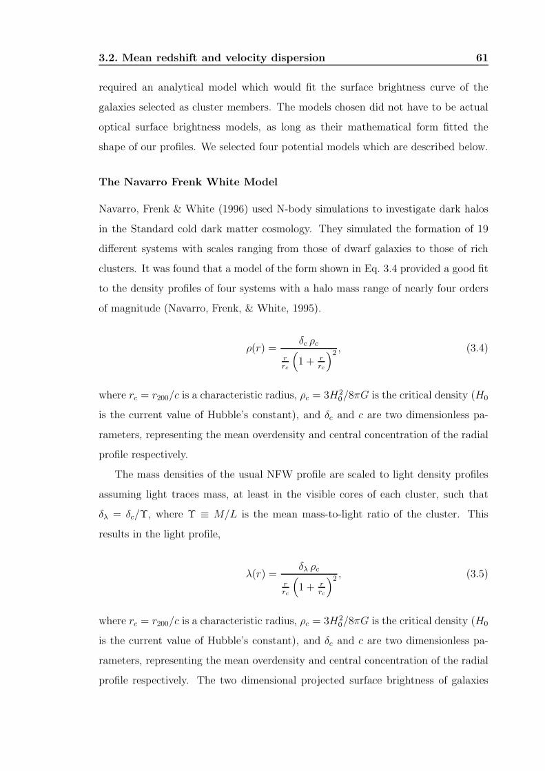
3.2. Mean redshift and velocity dispersion 61
required an analytical model which would fit the surface brightness curve of the
galaxies selected as cluster members. The models chosen did not have to be actual
optical surface brightness models, as long as their mathematical form fitted the
shape of our profiles. We selected four potential models which are described below.
The Navarro Frenk White Model
Navarro, Frenk & White (1996) used N-body simulations to investigate dark halos
in the Standard cold dark matter cosmology. They simulated the formation of 19
different systems with scales ranging from those of dwarf galaxies to those of rich
clusters. It was found that a model of the form shown in Eq. 3.4 provided a good fit
to the density profiles of four systems with a halo mass range of nearly four orders
of magnitude (Navarro, Frenk, & White, 1995).
ρ(r) =δc ρc
rrc
(
1 + rrc
)2 , (3.4)
where rc = r200/c is a characteristic radius, ρc = 3H20/8πG is the critical density (H0
is the current value of Hubble’s constant), and δc and c are two dimensionless pa-
rameters, representing the mean overdensity and central concentration of the radial
profile respectively.
The mass densities of the usual NFW profile are scaled to light density profiles
assuming light traces mass, at least in the visible cores of each cluster, such that
δλ = δc/Υ, where Υ ≡ M/L is the mean mass-to-light ratio of the cluster. This
results in the light profile,
λ(r) =δλ ρc
rrc
(
1 + rrc
)2 , (3.5)
where rc = r200/c is a characteristic radius, ρc = 3H20/8πG is the critical density (H0
is the current value of Hubble’s constant), and δc and c are two dimensionless pa-
rameters, representing the mean overdensity and central concentration of the radial
profile respectively. The two dimensional projected surface brightness of galaxies

3.2. Mean redshift and velocity dispersion 62
on the sky can be computed by integrating Eq. 3.4 according to the Abell integral
equation given by,
Λ (R) = 2
∫ ∞
R
ρ (r)r√
r2 − R2dr (3.6)
Bartelmann (1996) show this results in the projected surface brightness of,
Λ (R) =2ρcδλrc
x2 − 1f(x), (3.7)
with
f(x) = 1 − 2√x2−1
arctan√
x−1x+1
(x > 1) (3.8)
f(x) = 1 − 2√1−x2 arctan
√
1−x1+x
(x < 1)
f(x) = 1 (x = 1),
where x = r/rc, R being the projected radius from the centre of the cluster.
The Hernquist Model
Hernquist (1990) presented a potential density pair which closely approximates the
de Vaucouleurs R1/4 law for elliptical galaxies. A modification of the distribution of
Jaffe (1983) allowed the intrinsic properties and projected distributions to be eval-
uated analytically,
ρ(r) =M
2π
a
r
1
(r + a)3, (3.9)
where M is the total mass and a is a scale length. So as to be able to apply this
form to our optical data, in the same manner as for the NFW profile, we divide
through by a constant mass to light ratio, Υ, obtaining the relation,
λ(r) =L
2π
a
r
1
(r + a)3, (3.10)

3.2. Mean redshift and velocity dispersion 63
where L is the total light and a is a scale length. The two dimensional projected
surface brightness of galaxies on the sky can be computed by integrating Eq. 3.10
according to Eq. 3.6. This results in the projected surface brightness of,
Λ(R) =L
2πa2(1 − s2)2[(2 + s2) X(s) − 3], (3.11)
where s = R/a, R is the projected radius, L is the total light and
X(s) =1√
1 − s2sech−1s for (0≤s≤1) (3.12)
X(s) =1√
1 − s2sech−1s for (1≤s≤∞). (3.13)
The Plummer Model
The Plummer model was first used by Plummer (1911) to fit observations of globular
clusters and the density profile takes the form,
ρ(r) =3Mb2
4π
1
(b2 + r2)5/2, (3.14)
where M is the total mass of the cluster, and b is the Plummer radius, a scale pa-
rameter which sets the density of the cluster. In the same manner as the previous
models dividing by a constant mass to light ratio, Υ, results in the following light
profile,
λ(r) =3Lb2
4π
1
(b2 + r2)5/2, (3.15)
where L is the total light of the cluster. By integrating according to Eq. 3.6 the

3.2. Mean redshift and velocity dispersion 64
projected surface brightness profile can be obtained as,
Λ(R) =L
π
b2
(b2 + R2)2(3.16)
The standard “beta” model
Traditionally models assume that the intra-cluster X-ray emitting gas is isothermal
and that the gas and the galaxies are in hydrostatic equilibrium. King (1962) pre-
sented an analytical approximation to the isothermal sphere which is often referred
to as the standard beta model. The surface X-ray brightness at projected distance
R is given by
Σ(R) = Σ0[1 + (R/rc)2]−3β+0.5, (3.17)
where rc is the core radius of the gas distribution and β is the ratio of the specific
energy in galaxies to the specific energy in the hot gas. We can simply apply this
to our optical data fitting optical surface brightness instead of X-ray, such that,
Λ(R) = Λ0[1 + (R/rc)2]−3β+0.5. (3.18)
Model choice
Each of the above projected models were fitted to the observed optical surface bright-
ness profiles obtained from the SuperCOSMOS galaxy data as described in §3.2.1,
using the Numerical Algorithm Groups (NAG) E04JYF algorithm. The models were
fitted with the following variables
1. Beta model: from Eq. 3.18, three variables were fitted, a=Λ0, b=β and c=rc.
2. Hernquist model: from Eq. 3.11 two variables were fitted, a=L and b=2πa2.
3. NFW model: from Eq. 3.7 two variables were fitted, a=rc and b=ρc δλ.
4. Plummer model: from Eq. 3.16 two variables were fitted, a=L and b=b.

3.2. Mean redshift and velocity dispersion 65
Figure 3.16: Radial velocities of galaxies lying within the Abell radius of 2.14 h−1
70Mpc of each
galaxy cluster, belonging to the Pisces-Cetus supercluster, compiled from NED, 6dFGS, 2dFGRS
and SDSS. For each cluster, the mean recessional velocity is shown as a dotted line, and for those
with ≥12 redshifts, the velocity dispersion is shown on the upper right. (§3.2)

3.2. Mean redshift and velocity dispersion 66
Figure 3.17: Radial velocities of galaxies lying within the Abell radius of 2.14 h−1
70Mpc of each
galaxy cluster, belonging to the Horologium-Reticulum supercluster, compiled from NED, 6dFGS,
(Fleenor et al., 2005) and (Fleenor et al., 2006). For each cluster, the mean recessional velocity is
shown as a dotted line, and for those with ≥8 redshifts, the velocity dispersion is shown on the
upper right. (§3.2)

3.2. Mean redshift and velocity dispersion 67
Figure 3.18: Radial velocities of galaxies lying within the Abell radius of 2.14 h−1
70Mpc of each
galaxy cluster, belonging to the Shapley supercluster, compiled from NED, 6dFGS and ZCAT.
For each cluster, the mean recessional velocity is shown as a dotted line, and for those with ≥9
redshifts, the velocity dispersion is shown on the upper right. (§3.2)

3.2. Mean redshift and velocity dispersion 68
Figure 3.19: Radial velocities of galaxies lying with an extraction radius of each galaxy cluster,
belonging to the Shapley supercluster. The extraction radii are shown in the top centre of each
cluster panel and are expressed as a fraction of the Abell radius ( 2.14 h−1
70Mpc). All clusters
belong to the Shapley supercluster and galaxies are compiled from NED, 6dFGS and ZCAT. For
each cluster, the mean recessional velocity is shown as a dotted line, and for those with ≥9 redshifts,
the velocity dispersion is shown on the upper right. (§3.2)

3.3. Virial mass estimates 69
An additional constant term to represent foreground/background galaxies was also
added as an extra +c term to all the models. For the majority of the clusters the
galaxies were binned in variable radius annuli around the cluster centre, such that
each annulus contains an equal number of galaxies. The luminosity per unit area in
each annulus was then calculated to plot the surface brightness profiles. However, a
satisfactory fit could not be found for some clusters using this method. Therefore,
for these profiles, equal radius annuli with a variable number of galaxies were used.
From this process the NFW model was seen to be the best overall model, fitting
the most cluster profiles accurately. Therefore, the NFW fit was used as the final
fit all of the clusters profiles to enable estimates of their mass to be performed.
The resulting surface brightness profiles and their associated NFW fits are shown
in Appendix A, Appendix B, and Appendix C for the clusters of the Pisces-Cetus,
Horologium-Reticulum and Shapley superclusters respectively.
3.3 Virial mass estimates
The mass within a radius r from the centre of a cluster can be derived from the
modelled velocity dispersion and spatial density profiles λ (r) (Koranyi & Geller,
2000). On assumption of a constant mass-to-light ratio Υ ≡ M/L, the mass density
ρ (r) ≡ Υ λ (r), following (3.4), results in the enclosed mass profile,
M(< r) = 4πδcρcr3c
[
ln(1 +r
rc) − r/rc
1 + r/rc
]
. (3.19)
The core radius rc has already been found in the fitting of the surface brightness
profile as described in §3.2.1. The quantity δc and c are linked by the requirement
that the mean density within r200 should be 200×ρc, i.e.,
δc =200
3
c3
[ln(1 + c) − c/(1 + c)], (3.20)
where c = r200/rc. With the value of rc already being calculated the NFW model
would be completely specified if we knew r200.

3.3. Virial mass estimates 70
From the definition of r200, we have that,
ρ200 = 200ρc, (3.21)
where ρ200 is the density inside r200 and ρc is the critical density of the universe.
This leads to,
M200 = 200 × 4πr3200ρc
3, (3.22)
where M200 is the mass inside r200. It can be shown that the critical density of the
universe can be expressed as,
ρc =3H2
0 (1 + z)3
8πG, (3.23)
where H0 is Hubble’s constant, G is the gravitational constant and z is the redshift.
Substituting Eq. 3.23 into Eq. 3.22 gives,
M200 =100r3
200H20 (1 + z)3
G(3.24)
It can be shown that the virial mass can be defined as,
Mv =3σ2rv
G, (3.25)
where rv is the virial radius. Dividing Eq. 3.24 by Eq. 3.25 gives,
M200rv
Mνr3200
= 100H20
(1 + z)3
3σ2r
, (3.26)
where σ2r is the radial velocity dispersion of the cluster and rv is the approximate
virial radius determined by

3.4. A lower limit to the Mass of the Superclusters 71
rv ∼ π
2
N(N − 1)∑
i
∑
i<j R−1ij
, (3.27)
where N is the number of galaxies in the system. The summation is over all pairs
of galaxies (i, j) within the Abell radius, where the projected separation for each
pair is Rij (Binney & Tremaine, 1987). This should provide a radius at which most
cluster members are included.
The enclosed mass profile (3.19) can be used to find M200 and Mν in terms of δc.
The calculated cluster masses within the Abell radius of 2.14 h−170 Mpc, their core
radii and virial radii found from the model fitting, can be found in Table 3.1,Table 3.2
and Table 3.3 for the Pisces-Cetus. Horologium-Reticulum and Shapley supercluster
clusters respectively.
The virial estimate will fail to represent the gravitating mass of a cluster which
is very obviously in the process of rapid evolution, e.g. a collapsing or interacting
system, since the virial theorem does not strictly apply to systems whose moment
of inertia is significantly changing with time. Abell 87 is obviously such a system
and hence its mass has been omitted.
3.4 A lower limit to the Mass of the Superclusters
The sum of the individual virial masses of the clusters, as calculated in the previous
section, can be treated as a lower limit to the mass of each supercluster.
3.4.1 Pisces-Cetus supercluster
For the filament containing A85, we use a cylindrical column of length equal to
the sum of the distances between the constituent clusters from the MST analysis
equalling 47.9 h−170 Mpc. Adopting a radius of 6 h−1
70 Mpc (Approximately 3 Abell
radii) gives a volume of 5421 h−370 Mpc3, we obtain the total mass of the clusters as
2.44× 10¹⁵ h−170 M⊙. As discussed in section 3.2 Abell 87 is likely to be a filament of
galaxies rather than a cluster and therefore its mass is not included.

3.4. A lower limit to the Mass of the Superclusters 72
For the filament containing A133, we use a cylindrical column of length of
167.8 h−170 Mpc again equal to the sum of the cluster separations form the MST anal-
ysis. The radius of 6 h−170 Mpc for the cylinder gives a volume of 18996 h−3
70 Mpc3,
we obtain the total mass of the clusters as 3.88 × 10¹⁵ h−170 M⊙.
With the critical density of the universe having a value of ρc = 1.36 × 10¹¹ h270
M⊙ Mpc−3, these values for the mass of the Supercluster represent matter overdensi-
ties of δM ≡ ∆ρ/ρcrit >1.96 (over 5400 h−370 Mpc3) and δM >1.51 (over 19000 h−3
70 Mpc3)
for the A85-related and A133-related filaments respectively. Thus a mean for the
supercluster region of 1.74. These values are slightly lower than those found in the
core of the Shapley supercluster (5.2 over ∼ 22 h−1100 Mpc scale (Bardelli et al.,
2000)(extended sample)), (2.4 over ∼ 26 h−170 Mpc scale (Fabian, 1991)), (5.0 over
∼ 38 h−170 Mpc scale (Drinkwater et al., 2004)), (2.4 over ∼ 40 h−1
70 Mpc scale (Fleenor
et al., 2005)) and (5.4 over ∼ 30 − 46 h−170 Mpc scale (Proust et al., 2006)). The
cosmological significance of such overdensities in a supercluster filament has been
discussed in the literature (Raychaudhury, 1989; Ettori, Fabian, & White, 1997).
However, that these represent just the mass with some clusters omitted, no fila-
ment galaxies included, and that the matter density of the Universe is ΩM ∼ 0.3,
these amount to significant overdensities over very large volumes. This supports the
possibility that galaxies in these regions may evolve differently to galaxies which
are present in less dense regions and have different properties such as enhanced or
suppressed star formation.
3.4.2 Horologium-Reticulum supercluster
For the purposes of the estimate of a lower limit of the mass for the Horologium-
Reticulum supercluster we will take the super cluster to consist of those clusters that
are part of the main chain, joint by links of less than 20 h−1100 Mpc, represented by
solid lines in Fig. 3.8. The main chain spans from Abell 3089 through to Abell 3266,
containing 18 clusters (A3089, A3122, A3125, A3140, A3145, A3135, A3109, A3108,
A3100, A3123, A3120, A3110, A3078, A3074, A3125, A3158, A3164, A3225).
A lower limit of the mass of this structure found by summing all of the avail-
able masses of the constituent clusters results in a total mass of 6.60× 10¹⁵ h−170 M⊙.

3.5. Conclusions 73
Taking the volume of the supercluster to consist of a series of cylinders of radius
6 h−170 Mpc and length of the MST link between the clusters results in a total length
of 202.1 h−170 Mpc and a total volume of 22, 800 h−3
70 Mpc3. With the critical den-
sity of the universe having a value of ρc = 1.36 × 10¹¹ h270 M⊙ Mpc−3, this value
for the mass of the Supercluster represents a matter overdensity of δM >2.1 (over
23, 000 h−370 Mpc3)
Again given that these represent just the mass with some clusters omitted, no
filament galaxies included, and that the matter density of the Universe is ΩM ∼0.3,
these amount to significant overdensities and the possibility of environmental effects
on the evolution of galaxies in the region.
3.4.3 Shapley supercluster
For the Shapley supercluster the main chain consisting of all clusters joined by
links of less than 20 h−1100 Mpc included all clusters accept for A1631, A1644 and
A1709. The total length of the MST links between these clusters was 195.31 giving
a volume of 22, 089 h−370 Mpc3 for the adopted cylinder radius of 6 h−1
70 Mpc. The
total mass is 1.2 × 10¹⁶ h−170 M⊙. With the critical density of the universe having a
value of ρc = 1.36× 10¹¹ h270 M⊙ Mpc−3, this value for the mass of the Supercluster
represents a matter overdensity of δM >4.06 (over 22, 000 h−370 Mpc3).
This value is even higher than the previous two superclusters making the super-
cluster even more likely to effect the evolution of galaxies.
3.5 Conclusions
We have used survey redshifts (mainly from 2dFGRS, 6dFGS, SDSS, NED and
ZCAT) and photometry (from SuperCosmos) of galaxies belonging to the clusters
belonging to three superclusters to investigate its nature, extent and orientation.
The Pisces-Cetus supercluster consists of two main filaments, consisting of 11
and 5 clusters respectively, at mean redshifts of z =0.0625 and 0.0545 respectively.
The Horologium-Reticulum supercluster consists of 33 clusters of galaxies at a mean
redshift of z =0.0670 (MST maximum edge length = 25 h−1100 Mpc) and mainly

3.5. Conclusions 74
extends in the radial direction. Finally the Shapley supercluster consists of 29
clusters at a mean redshift of z =0.0476 MST maximum edge length = 25 h−1100 Mpc).
While there is some suggestion of filamentary structure in all three of the super-
clusters the position of the Pisces-Cetus supercluster with some coverage in both
the SDSS and 2dFGRS leads to the most compelling evidence. Most of chain A of
the Pisces-Cetus supercluster lies in the 2dFGRS region, and gives us a remarkable
three-dimensional view of a string of clusters, with groups delineating the filamen-
tary structure. Chain B, partially covered by the Sloan Digital sky survey, contains
the clusters A85 & A87, for which independent evidence exists (from X-ray obser-
vations) of collapse along the filament.
Virial masses were calculated from NFW fits to surface brightness profiles and
velocity dispersions for the constituent clusters, the sum of these masses being taken
as a lower limit to the mass of each of the superclusters. These were found to be
6.0 × 10¹⁵ h−170 M⊙ and 5.2 × 10¹⁵ h−1
70 M⊙ respectively for the chain A and chain B
of the Pisces-Cetus supercluster, 6.6 × 10¹⁵ h−170 M⊙ for Horologium-Reticulum and
1.2 × 10¹⁶ h−170 M⊙ for Shapley. These correspond to mass overdensities of δM >1.5,
δM >2.0, δM >2.1 and δM >4.1, for Pisces-Cetus chain A, Pisces-Cetus chain B,
Horologium-Reticulum and Shapley respectively.
These values indicate that in all three superclusters, it is likely that the systems
are just in the linear regime or have just left it. Furthermore, these overdensities
suggest that the regions may have different environmental conditions to other regions
and hence may have different effects on the evolution of galaxies.
Ever since the discovery of the “Great Wall”(Geller & Huchra, 1989), which
seemed to be a structure almost < 200 h−170 Mpc long, the discovery of comparable
structures have been claimed at higher redshift (e.g., Bagchi et al., 2002; Brand
et al., 2003; Miller et al., 2004). To be cosmologically significant, it is necessary
to show that these large structures are gravitationally bound, which is difficult to
demonstrate. In this work, we have found cluster filaments between approximately
50 h−170 Mpc and 130 h−1
70 Mpc long. This is consistent with statistical analyses of the
LCRS and 2dF redshift surveys, which indicate that the scale of homogeneity sets
in beyond the scale of ∼ 100 h−170 Mpc or so.

3.5. Conclusions 75
A limited X-ray analysis of the LX−σ relation in the clusters of the Pisces-Cetus
supercluster, based on literature X-ray data can be found in Appendix D.

Chapter 4
Benjamin Disraeli: “There are three kinds of lies: lies, damned lies, and statistics.”
Star formation in the Pisces-Cetus
supercluster
4.1 Introduction
Studies of the environmental effects on galaxy evolution in the past have shown that
star formation is suppressed in the cores of rich clusters (Dressler, 1980; Couch &
Sharples, 1987; Balogh et al., 1998). More recently, from the high-quality spectra
of the 2dFGRS and SDSS archives, the difference between the properties of star-
forming and quiescent galaxies have been further characterised, and shown to depend
on the local density of galaxies. For instance, studies (Lewis et al., 2002; Gomez et
al., 2003; Balogh et al., 2004) identifying star formation activity with the equivalent
width of the Hα emission line W (Hα), show that the fraction of galaxies with
W (Hα)>4 A steadily declines with increase in the local three-dimensional density
of galaxies. Kauffmann et al. (2004) show similar effects, with the star formation
history being quantified from line indices measured elsewhere in the spectrum as
well, including the Hδ absorption line and the strength of the 4000A break.
In the hierarchically merging scenario supported by large-volume numerical sim-
ulations such as Jenkins et al. (1998), much of this merger-driven evolution in the
history of a galaxy is expected to occur in small groups forming in and falling along
a supercluster filament towards regions of higher density. In the absence of direct
mergers, the close encounters between galaxies brought closer by dynamical friction,
76

4.2. Star formation within Pisces-Cetus supercluster filaments 77
can lead to galaxy harassment, which can also play a very important role in galaxy
evolution, and can affect the star formation properties of galaxies.
To investigate the star formation rate (SFR) within the galaxies that form the
Pisces-Cetus supercluster we use the 2dFGRS η parameter as discussed in Chapter
2.
4.2 Star formation within Pisces-Cetus superclus-
ter filaments
A supercluster filament is a snapshot of a cluster in formation, and the study of the
properties of galaxies as a function of position along a filament is expected to provide
insights into the processes involved in galactic evolution and cluster formation. This
section looks at galaxies in a few filaments of the Pisces-Cetus supercluster.
The clusters comprising the Pisces-Cetus supercluster, taken from the minimal
spanning tree (MST) analysis of Raychaudhury et al. (2007), form the core of our
sample. The filamentary nature of the region can clearly be seen in the distribution
of galaxies in the groups in Fig. 4.2, where the 2dFGRS galaxies within 1840 kms−1
(three times the velocity dispersion of the clusters belonging to the supercluster),
are plotted. The 2PIGG groups found within the same velocity bounds (Eke et al.,
2004), also show the same large-scale structure. The rich clusters, plotted as large
circles on the same plot, can be seen to be mostly along these filaments forming the
supercluster structure.
4.2.1 Filament membership
Our sample of galaxies was taken from the 2PIGG (Eke et al., 2004) subsample of
the 2dFGRS comprising 191,328 galaxies. This leaves out about 20 % of galaxies
in the parent sample in under-sampled regions and ensures a uniform completeness
limit all over the survey. This enables comparisons with 2PIGG statistics to be
made without bias. Hereafter, 2dFGRS refers to this subsample.
From this subsample, galaxies which belong to the three most prominent fila-

4.2. Star formation within Pisces-Cetus supercluster filaments 78
Figure 4.1: (a, Left) All 2dFGRS Galaxies within 1840 km s−1 (3σ) of the mean recessional
velocity of the Pisces-Cetus supercluster. The filamentary structure is clearly visible. (§4.2)
Figure 4.2: Clusters of galaxies belonging to Pisces-Cetus supercluster filaments within the
2dFGRS region and within 1840 km s−1 (3σ) of the mean supercluster velocity. The largest circles
represent Abell clusters, and the medium-sized ones are supplementary Abell and Edinburgh-
Durham clusters within the same redshift range. The groups of galaxies (Eke et al., 2004, 2PIGG)
within the same velocity bounds, identified from a friends-of-friends analysis of the 2dFGRS are
shown as the smallest circles. (§4.2)

4.2. Star formation within Pisces-Cetus supercluster filaments 79
Figure 4.3: The 2dFGRS galaxies that form the three filaments as defined in the text are shown
as crosses. All galaxies within the 2dFGRS in the region are shown as dots. (§4.2.1)
ments, longer than 20 h−170 Mpc, seen in Fig. 4.2, namely those joining A2800-A2734,
A2734-E0365 and E0365-A2716, were extracted.
We define the extent of each filament as an prolate spheroid, with the centres of
the two clusters involved being at each end, the distance between them being the
major axis of the spheroid, and 6 h−170 Mpc being the semi-minor axis. All galaxies
falling inside this spheroid were taken to be members of the filament. So as to not
omit cluster galaxies at each end of the filament, we added the galaxies found, from
a percolation analysis, to belong to the corresponding 2PIGG “group” in (Eke et al.,
2004). The resulting 965 filament members can be seen in Fig. 4.3.
The distance between two clusters, and between a galaxy and a cluster, was
calculated as the co-moving proper distance between them (see Hogg, 1999). We
used the measured redshift of each galaxy as a measure of its distance from us,
except if it is a member of a rich cluster, where the mean redshift of the cluster was
used.
Fig 4.2.1 shows the distribution of the 2dFGRS galaxies for the 2PIGG group
corresponding to Abell 2734. The red circle in the left hand plot shows the Abell
radius (2.14 Mpc h−170 ). This demonstrates that simply taking cluster members to
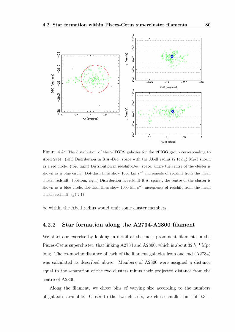
4.2. Star formation within Pisces-Cetus supercluster filaments 80
Figure 4.4: The distribution of the 2dFGRS galaxies for the 2PIGG group corresponding to
Abell 2734. (left) Distribution in R.A.-Dec. space with the Abell radius (2.14 h−1
70Mpc) shown
as a red circle. (top, right) Distribution in redshift-Dec. space, where the centre of the cluster is
shown as a blue circle. Dot-dash lines show 1000 km s−1 increments of redshift from the mean
cluster redshift. (bottom, right) Distribution in redshift-R.A. space , the centre of the cluster is
shown as a blue circle, dot-dash lines show 1000 km s−1 increments of redshift from the mean
cluster redshift. (§4.2.1)
be within the Abell radius would omit some cluster members.
4.2.2 Star formation along the A2734-A2800 filament
We start our exercise by looking in detail at the most prominent filaments in the
Pisces-Cetus supercluster, that linking A2734 and A2800, which is about 32 h−170 Mpc
long. The co-moving distance of each of the filament galaxies from one end (A2734)
was calculated as described above. Members of A2800 were assigned a distance
equal to the separation of the two clusters minus their projected distance from the
centre of A2800.
Along the filament, we chose bins of varying size according to the numbers
of galaxies available. Closer to the two clusters, we chose smaller bins of 0.3 −

4.2. Star formation within Pisces-Cetus supercluster filaments 81
Figure 4.5: For the filament of galaxies linking A2734 and A2800, the mean η is plotted as a
function of the distance from the centre of A2734. The “field” value, the mean η for all galaxies of
the 2dFGRS, is around zero. The bottom panel shows the fraction of passive galaxies (η <−1.4)
in each bin. It can be seen, as expected, that the SFR is lowest at the cores of the two rich
clusters, where the number of passive galaxies is the highest. The mean η seems to peak between
3–4 h−1
70Mpc from each end. (§4.2.2)
0.6 h−170 Mpc to sample the rapid variation of SFR within the virial radius of the
cluster. For each bin, the the mean distance of all member galaxies, and the mean
η, were calculated.
Fig. 4.5 shows the resulting plot of mean η as a function of distance from A2734.
We also plot, in the bottom panel, the fraction of passive (η<−1.4) galaxies in each
bin. It can be seen, as expected, that the SFR is minimum at the cores of the two
rich clusters, where the number of passive galaxies is the highest. The mean value
of the η parameter increasing with distance to approximately the field value (the
mean η for all galaxies of the 2dFGRS is around zero).
However, it can also be seen that between 3–4 h−170 Mpc from the centre of A2734
there is a peak in the mean η. There is another peak at the A2800 end of the plot
at a slightly closer distance from the cluster centre. Although within errors one of
them does not rise above the field, there is enough of an indication of a peak to
warrant further investigation by increasing numbers. To investigate the reality of
the signal, we will now stack all three filaments in our sample, and fold Fig. 4.5 such

4.2. Star formation within Pisces-Cetus supercluster filaments 82
Figure 4.6: The distribution of passive (η<−1.4) galaxies shown as filled circles and star forming
(η>−1.4) galaxies shown as crosses in the region surrounding Abell 2800. Only galaxies belonging
to the A2734–A2800 filament are shown. The concentric circles are at 1 h−1
70Mpc intervals. (§4.2.2)
that we consider distances along the filament from the nearest cluster.
Fig. 4.6 and Fig. 4.7 show the distribution of the passive and star forming galaxies
for Abell 2800 and Abell 2734 respectively. The concentric circles are at 1 h−170 Mpc
intervals and it can be seen that in the 3–4 h−170 Mpc annulus there are more star
forming than passive galaxies for both clusters.
4.2.3 Star formation properties of galaxies in all three fila-
ments combined
The distance of each of the filament members from the nearest of the two clusters
at either end was calculated using the same method as above.
Here we combine the three filaments longer than 20 h−170 Mpc, namely those
joining A2800–A2734, A2734–E0365 and E0365–A2716, seen in Fig. 4.3. All galaxies
belonging to the three filaments were grouped in bins of varying size according to
their distance from the nearest cluster (representing the extremities of the filaments).
As above, we plot the mean value of η and the fraction of passive galaxies in each
bin in Fig. 4.8. For comparison between the trend with distance for the filament
galaxies with galaxies elsewhere, we compute “field” values from the whole 2dFGRS,

4.2. Star formation within Pisces-Cetus supercluster filaments 83
Figure 4.7: The distribution of passive (η<−1.4) galaxies shown as filled circles and star forming
(η>−1.4) galaxies shown as crosses in the region surrounding Abell 2734. Only galaxies belonging
to the A2734–A2800 filament are shown. The concentric circles are at 1 h−1
70Mpc intervals. (§4.2.2)
Table 4.1: Virial radii for Pisces-Cetus filament clusters
Cluster σ Virial radius
(kms−1) (Mpc)
A2800 567 1.62
A2734 848 2.42
A2716 812 2.32
E0365 442 1.26
where distances are calculated from the nearest 2PIGG group of ≥ 30 members (the
equivalent of a rich cluster), shown as the dashed line.
While the “field” values of mean η increase steadily with distance from the centre
of the nearest cluster, the galaxies in the filaments, binned in the same way, show a
peak between 3–4 h−170 Mpc, confirming our finding from the single filament above.
A rough estimate of the virial radius of each of the clusters is calculated using
the formula of Girardi et al. (1998), Rv = 0.002σ(h−1Mpc), where σ is the one-
dimensional velocity dispersion. These are shown in Table 4.1.
The peak region therefore corresponds to about 2 virial radii. A corresponding
dip in the percentage of passive galaxies is also seen at this distance. Of course, star

4.2. Star formation within Pisces-Cetus supercluster filaments 84
Figure 4.8: (a, Top) For the three filaments combined, the mean η as function of distance from
the nearest cluster is shown. The dashed line shows the mean η as function of distance from the
nearest 2PIGG group with ≥ 30 members for all 2dFGRS galaxies. (b, Bottom) For the same
galaxies as above, the fraction of these galaxies with an η<−1.4 is shown as a function of distance
from the nearest cluster. The dashed line showing the same fraction as a function of distance from
the nearest 2PIGG group with ≥ 30 members for the whole 2dFGRS. (§4.2.3)
formation is suppressed as the galaxy approaches the core of the cluster, leading to
a low mean η and a higher fraction of passive galaxies interior to this distance. The
cause of the enhanced star formation is discussed in more detail in (§4.3).
To get a better picture of how the values of η for the individual galaxies contribute
to the means, a histogram of η in each of the 8 bins is shown in Fig. 4.9. It can be
seen that the large peak of galaxies at the lowest levels of SFR seen in the first three
bins is missing in bins 5 and 6. This combines with a relatively high percentage of
galaxies having high η values of above 0 is consistent with the corresponding peak
in the mean η of Fig. 4.8.
4.2.4 Star formation in high and low velocity dispersion
clusters
If tidal forces were an important influence on the peak in star formation, we would
expect that the position of any region of enhanced star formation would vary ac-

4.2. Star formation within Pisces-Cetus supercluster filaments 85
Figure 4.9: For the three filaments combined, histograms of the galaxy η’s in each of the 8
distance bins. (§4.2.3)
cording to the velocity dispersion of the cluster that it was nearest to. Tidal forces
are proportional to M/R3, where M is the mass of the cluster and R the distance
from the cluster at which tidal forces are encountered. Since the mass of a cluster is
proportional to σ2Rv, where σ is the velocity dispersion, you would expect galaxies
falling into clusters of larger velocity dispersion to encounter tidal forces at larger
distances.
We therefore split the four clusters that form our filaments into those with high
velocity dispersions (A2716 = 812 km s−1, A2734 = 848 km s−1) and those with low
velocity dispersions (A2800 = 567 km s−1, E0365 = 426 km s−1). Distances from
the clusters in each of the two samples were then calculated for the galaxies from
the three filaments. Fig. 4.10 shows the resulting values for mean η as a function
of distance for the high and low velocity dispersion cluster samples. It can be seen
that there is no significant difference in the position of the low velocity dispersion
cluster peak in mean η (filled circles) and the peak in the high velocity dispersion
cluster peak (open circles).

4.2. Star formation within Pisces-Cetus supercluster filaments 86
Figure 4.10: (a, Top) For the three filaments combined, the mean η as function of distance from
the nearest high or low velocity dispersion cluster is shown. Distances from low velocity dispersion
clusters (A2800 and E0365) are shown as filled circles, while distances from high velocity dispersion
clusters (A2734 and A2716) are shown as open circles. The dashed line shows the mean η as
function of distance from the nearest 2PIGG group with ≥ 30 members for all 2dFGRS galaxies.
(b, Bottom) For the same galaxies as above, the fraction of these galaxies with an η<−1.4 is shown
as a function of distance from the nearest cluster. The dashed line showing the same fraction as
a function of distance from the nearest 2PIGG group with ≥ 30 members for the whole 2dFGRS.
(§4.2.4)

4.2. Star formation within Pisces-Cetus supercluster filaments 87
Figure 4.11: Star formation in giant galaxies (MB ≤−20) vs that in dwarfs (−20<MB≤−17.5),
in the three filaments combined. (a, Top) The mean star formation rate parameter η is shown as
function of distance from the nearest cluster, for dwarfs (open triangles) and giants (filled circles).
(b, Bottom) The fraction of these galaxies with η <−1.4 is shown as a function of distance from
the nearest cluster. (§4.2.5)
4.2.5 Star formation in giant and dwarf galaxies
As samples of galaxies with estimated star formation properties grow larger, it would
become easier to study the relation between star formation in a galaxy and various
properties of its environment, and those of the galaxies themselves (e.g., Haines et
al., 2006a).
Here, in Fig. 4.11, we break up the galaxies plotted above in Fig. 4.8 into two
subsamples: giant galaxies (MB ≤−20) and dwarf galaxies (−20<MB ≤−17.5). As
a result there are are 119 giants and 846 dwarfs in the three filaments used above.
As in Fig. 4.8, we plot the mean value of η as a measure of star formation, and the
fraction of passive galaxies, as a function of their distance from the nearest cluster,
with dwarfs plotted as open triangles and giants as filled circles.
It seems that the peak in mean η seen in Fig. 4.8, between 3 − 4 h−170 Mpc, is
almost entirely due to enhanced star formation in dwarfs, indeed there are no passive
dwarf galaxies in the bin containing the peak in mean η.
It can be seen in Fig. 4.12, especially for the giant galaxies that there are more

4.2. Star formation within Pisces-Cetus supercluster filaments 88
Figure 4.12: The distribution of giant (MB ≤−20) and dwarf (−20 < MB ≤−17.5) galaxies,
in the three filaments combined in R.A.-Dec. space. Also shown is the current star formation of
these galaxies with passive (η <−1.4) galaxies shown as blue and star forming (η <−1.4) as red.
The green circles show the virial radius of each cluster. (§4.2.5)
passive galaxies within the virial radius than star forming. The virial radii are taken
from Table 4.1.
While the differences in the populations would appear to be real it is worth re-
membering that the populations were determined from the blue magnitudes. The
blue magnitude will be boosted by star formation and therefore the high η galaxies
will have preferentially higher blue magnitudes, This will result in some dwarf galax-
ies being shifted into the giant population. This might explain why our populations
overlap at lower radii unlike the completely separate lines of Haines et al. (2006a)
who use SDSS R band data. Ideally K-band magnitudes would have been used to
separate our populations, but we do not have such magnitudes available from the
2MASS survey for all our galaxies.
4.2.6 Star formation in Groups
The suppression of star formation with increasing local density of galaxies has been
observed to occur in giant galaxies at very low values of the local projected density
(∼ 1 h−170 Mpc−2) (e.g. Lewis et al., 2002; Gomez et al., 2003), which are typical
of densities well-outside the virialised regions in clusters, indicating that the cause

4.2. Star formation within Pisces-Cetus supercluster filaments 89
does not lie entirely in the influence of the cluster environment. One suggestion
is that much of the evolution of galaxies occurs in groups during their life on the
filaments, before the groups are assimilated in clusters. Evidence supporting this
is found in the virialised structure of some galaxy groups (O’Sullivan, Forbes, &
Ponman, 2001). If so, the trend seen in the previous section would be different for
filament galaxies that belong to groups and those that are relatively isolated.
We divide our sample of galaxies that are members of the three Pisces-Cetus
filaments into those that belong to groups (2PIGG groups with 4 or more mem-
bers, (Eke et al., 2004), and relatively isolated galaxies, which are galaxies that are
not members of 2PIGG groups. Fig. 4.13 shows the variation of mean η and the
fraction of passive galaxies for these two subsamples, as a function of the distance
from the nearest cluster for the filament galaxies. There is a large scatter in the
points corresponding to non-group galaxies (representing only 8% of the total num-
ber in the sample). There is very weak evidence that the peak in mean η occurs in
groups at smaller distances than in the non-group galaxies, which in general have a
higher fraction of star forming galaxies. However, as non-group galaxies can not be
found within approximately 3 h−170 Mpc of the cluster centres there will be a consid-
erable selection bias against having a peak in star-formation in non-group galaxies
at 3 h−170 Mpc or less.
Fig. 4.14 compares the same quantities for galaxies that belong to groups (2PIGG,
N ≥4) in these three filaments to similar group galaxies elsewhere in the 2dFGRS.
The black dots represent the variation of mean η and passive galaxy fraction as a
function of distance from the nearest cluster in the 2dFGRS. The plots suggest that
in the sample representing the whole 2dFGRS the SFR is more or less uniform in
all group galaxies irrespective of their distance from the nearest cluster, except for
those galaxies within the virial radii of clusters. In sharp contrast, the trend we find
of a peak in SFR between 3 − 4 h−170 Mpc is seen in the group galaxies that belong
to filaments.
To investigate whether the groups that we were comparing the SFR in were the
same basic entities in the three filaments and in the whole 2dFGRS, we have plotted
histograms of the richness and velocity dispersion for these group samples. These

4.2. Star formation within Pisces-Cetus supercluster filaments 90
Figure 4.13: (a, Top) The mean value of the η as a function of distance from the nearest
cluster, for all galaxies in the three filaments combined. Galaxies that are members of groups
(2PIGG groups with N ≥ 4) are shown as filled circles while galaxies that are not part of a group
as squares. (b, Bottom) The fraction of filament galaxies with η<−1.4 is plotted as a function of
distance from the nearest cluster for the same samples. (§4.2.6)
Figure 4.14: Star formation in galaxies in 2dFGRS groups: those in filaments vs the entire
2dFGRS: (a, Top) The mean value of the η as a function of distance from the nearest cluster.
Filament galaxies that are members of groups (2PIGG groups with N ≥ 4) are shown as crosses.
This is compared to a sample of ALL galaxies in the 2dFGRS that are members of similar 2PIGG
groups (dashed line). The peak in η is not seen in the latter category. (b, Bottom) The fraction
of filament galaxies with η <−1.4 as a function of distance from the nearest cluster for the same
samples. (§4.2.6)

4.2. Star formation within Pisces-Cetus supercluster filaments 91
Figure 4.15: (a, Left) Histograms of the relative number of groups with richness 0-25 for
groups (2PIGG groups with N ≥ 4) within the 3 filaments of the Pisces-Cetus supercluster (green)
and groups within the entire 2dFGRS (Red). (b, Right) Histograms of the relative number of
groups with velocity dispersion 0-1000 Kms−1 for groups within the 3 filaments of the Pisces-
Cetus supercluster (green) and groups within the entire 2dFGRS (Red). (§4.2.6)
histograms can be seen in Fig 4.15a and Fig 4.15b. It can be seen that there is some
evidence that the group galaxies in the filaments (green histograms) have richer
groups. There is also marginal evidence that the group galaxies in the filaments
have larger velocity dispersions in the range up to 400 kms−1. This may be due
to the filamentary structure of the region causing the percolation algorithm used in
finding the groups to include more group members and hence the groups to have
larger velocity dispersions. Due to this effect and the marginal results of our group
work we have chosen not to emphasise the group results.
4.2.7 Welch’s test results
Given two data sets, each characterised by its mean, standard deviation and number
of data points, we can use some kind of t test to determine whether the means are
distinct, provided that the underlying distributions can be assumed to be normal.
All such tests are usually called Student’s t tests, though strictly speaking that
name should only be used if the variances of the two populations are also assumed
to be equal. In our case the variances of our means do not have the same variance
and so we use a variant of the Student’s t tests, Welch’s t test. Welch’s t test is
an adaptation of Student’s t-test intended for use with two samples having unequal

4.2. Star formation within Pisces-Cetus supercluster filaments 92
Table 4.2: Welch’s test results for Pisces-Cetus filamentsFigure Probability
number 1 2 3 4 5 6 7 8 9 Joint (4-9)
Fig. 4.8 7.6E-5 2.4E-3 0.53 0.93 0.14 0.74 0.83 0.36 0.42 0.01
Fig. 4.10 ∗ 5.2E-5 0.027 0.006 0.004 0.83 0.28 0.25 0.93 0.67 1.4E-4
Fig. 4.11 0.57 0.89 0.72 0.02 0.0076 4.4E-6 0.17 0.001 1.14E-13
Fig. 4.13 0.71 0.46 0.20 0.16 0.01
Fig. 4.14 3.1E-7 3.1E-5 0.53 0.61 0.28 0.38 0.04 0.77 0.74 1.4E-3
(*) Note that in the case of Fig. 4.10, the test is performed between the low and high velocity dispersion samples,
represented by the filled and open circles respectively.
variances, with the statistic given by,
t =Xa − Xb
[var(Xa)/Na + var(Xb)/Nb]1/2, (4.1)
where Xa is the mean value in dataset 1, Xb is the mean value in dataset 2, var(Xa)
is the variance of dataset 1, var(Xb) is the variance of dataset 2, Na is the number
of data in datset 1 and Nb is the number of data in datset 2. The number of degrees
of freedom, v, is given by,
vXa−Xb=
[
var(Xa)Na
+ var(Xb)Nb
]2
[var(Xa)/Na]2
Na−1+ [var(Xb)/Nb]2
Nb−1
, (4.2)
The above formulas as part of the “tutest” routine from Press et al. (1992) were
applied to the mean η in each bin of our SFR as a function of distance from the
centre of a cluster and gave the results seen in Table 4.2. The joint probability
for the filament region outside of the cluster radius (bins 4-9) is also shown in
Table 4.2. It can be seen that for Fig. 4.8 the point at which the SFR of the filament
galaxies peaks, has a probability of 0.14 of the means being equal. This corresponds
approximately to a 1.5 σ result, which while not overwhelmingly significant, the
result persisted in various subsets of the Pisces-Cetus sample, i.e. the filaments
taken independently, as well as the high and low velocity dispersion cluster samples.
With the sample drawn from the entire 2dFGRS having no such result this suggests
that the result may be stronger than that which the statistics show. The first 4 bins
of Fig. 4.10 show significant differences between the high and low velocity dispersion
clusters (see §4.3) with three of the bins having probabilities of approximately 3 σ

4.3. Discussion 93
or greater. The joint probabilities shows that the populations that are the most
different to each other are the dwarf and giant samples of Fig. 4.11.
4.3 Discussion
The most striking of our results are those seen in Fig. 4.8, where we look at galaxies
which are members of filaments joining pairs of rich clusters of galaxies. We see a
decline in SFR in these galaxies, from the filament environment on the periphery of a
cluster, to the galaxies in the cluster core, that indicate a physical mechanism at work
that quenches star formation progressively as a galaxy approaches the core of the
cluster potential well. This trend is consistent with that seen in other environmental
studies (e.g., Balogh et al., 1998; Moran et al., 2005). However the unusual feature
in our own case is that, on top of this decline we see a nearly instantaneous effect
which causes a burst of star formation at ∼ 3 h−170 Mpc from its centre, which is
about 1.5–2 times the virial radius of the cluster.
It has been shown that galaxies can be surrounded by a halo of hot gas with
a temperature of up to a few million degrees Kelvin (e.g., Pedersen et al., 2006).
However, it is likely that many more galaxies have a warm halo of gas with a
temperature of a few hundred thousand degrees Kelvin which is too cool to be seen
in X-ray detections and too warm to be seen in radio detections. This halo of
warm gas would provide a store of gas which can be used as fuel for continued star
formation in galaxies.
As galaxies approach the gravitational potential well of cluster, they will start to
encounter the Intracluster Medium (ICM), possibly at a distance much larger than
the virial radius. Approaching the outer regions of the cluster along a filament,
at the same time, the density of galaxies will begin to increase rapidly. At this
stage the galaxies will start to lose their warm gas haloes through evaporation and
possibly ram pressure stripping, as the gaseous halo of the galaxy interacts with the
hot ICM. This will lead to a steep decline in the SFR of galaxies between about
∼ 3 h−170 Mpc, progressively to the centre. This is seen in Fig. 4.8. When the galaxies
reach the very dense core region of the clusters at < 1 h−170 Mpc, galaxy harassment

4.3. Discussion 94
(Moore et al., 1999) will become an important effect. With a lot of their gas already
removed by this stage, star formation will not be induced by the harassment, and
the remaining gas of the galaxy will now be stripped, leading to the observed steep
dip in SFR in the first two bins from the centre of the cluster.
Superposed on this trend, a rapidly acting process such as galaxies experiencing
the ICM for the first time or galaxy harassment are the most likely candidates for
our observed sudden burst in SFR at ∼ 3 h−170 Mpc from the cluster. As galaxies
just start to encounter the ICM they will not yet have had their gas stripped or
evaporated, but the interaction with the ICM will lead to shocks leading to a burst
of star formation. Similarly, with their gas still intact, galaxy harassment may lead
to density fluctuations in the gas which may trigger a burst of star formation. In
the infall region of the cluster at a few h−170 Mpc, the galaxies will just have started
to encounter the density of galaxies needed for galaxy harassment to become an
important factor. The sharpness of the peak in SFR is another indicator that galaxy
harassment may be important, since Moore et al. (1999) show that harassment is a
rapid effect.
The effects of “backsplash” (Gill, Knebe, & Gibson, 2005) which are strongest in
approximately the 1− 2 h−170 Mpc range are not likely to have a strong effect on our
peak in SFR, which is further out, but it may mean that the increase in SFR in some
galaxies in the sharp peak region may be even stronger than our mean suggests.
Moran et al. (2005) also observe a peak in SFR in the approach to the rich cluster
CL0024 at z=0.4. Their peak however is observed at 1.8 h−170 Mpc, i.e. at approxi-
mately half the distance of our peak. It is possible the discrepancy between the two
may stem from the fact that we are looking at galaxies falling into clusters along
filaments. In the case of CL0024, galaxies are falling into the cluster isotropically,
while ours are falling in along a denser filament of galaxies, which can lead to a
higher local density. This may lead to our galaxies encountering galaxy harassment
further from the cluster core.
Our peak in SFR may even contribute to our steep gradient within ∼ 3 h−170 Mpc,
making it steeper. The galaxies that are star forming will have had their gas tem-
perature raised and thus when they encounter the ICM they will be more prone to

4.3. Discussion 95
evaporation and stripping and hence have a rapidly decreasing SFR (for a similar
effect on groups see Rasmussen, Ponman, & Mulchaey, 2006).
The principal component analysis used in obtaining the η parameter will not
have removed contributions from active galactic nuclei (AGN). It therefore remains a
possibility that our peak in SFR is due to AGN activity rather than conventional star
formation. In fact this would be fairly consistent with the X-ray results of Ruderman
& Ebeling (2005) who find a prominent spike in the number of cluster AGN at
∼ 2.5 h−170 Mpc. However, the detection of X-ray AGN does not necessarily confirm
the presence of an optical AGN (Shen et al., 2007) and the above arguments are more
suggestive of galaxy harassment being the dominant effect leading to starbursts.
Fig. 4.10 shows that there is no real difference in the position of the peak in SFR
in the infall regions of high or low velocity dispersion clusters. Therefore, either
the enhanced star formation that we are seeing is not due to the tidal effects of
the cluster or the tidal forces are being masked by stronger effects such as those
described above. However this plot does show a marked difference between the low
and high velocity dispersion distributions in the first 4 bins. In this region the high
velocity dispersion clusters are at significantly lower SFRs, this is consistent with
the higher velocities resulting in more ram pressure stripping and hence there is less
gas available for star formation.
Fig. 4.11 shows that our dwarf galaxies generally have a higher SFR than the
giant galaxies. This is consistent with the results of Haines et al. (2006a) and
Moran et al. (2005). This also provides more evidence for galaxy harassment being
the dominant influence on the burst in star formation, dwarf galaxies are expected
to be more vulnerable to galaxy harassment than giants. Moran et al. (2005) shows
this, where almost all the galaxies in their peak in the [OII] equivalent width are
dwarfs.
The fact that our peak in SFR is mainly due to the dwarf galaxies also means
that the burst in SFR is unlikely to be due to merging of galaxies. The small merger
cross sections of dwarfs make them unlikely candidates for mergers.
Fig. 4.13 suggests that non group galaxies may have higher SFR at greater
distances from the cluster core. However, the low numbers of galaxies used here

4.4. Conclusions 96
make the trend inconclusive. This will be investigated with a larger sample of
galaxies in Chapter 5.
4.4 Conclusions
We investigated the environmental dependence of star formation within a superclus-
ter environment. We have done this by finding the variation of the η parameter with
distance from cluster centres along filaments of galaxies joining rich clusters.
For galaxies belonging to three filaments (each over 20 h−170 Mpc long), connecting
three pairs of rich clusters, we have looked at the variation of the mean η parameter
with distance along the filaments, in bins of one to a few h−170 Mpc, starting from the
cores of the rich clusters out to the sparser reaches of the filament. We have also
looked at similar dependence on distance of the fraction of passive galaxies (η<−1.4,
which is equivalent to the equivalent width of the Hα emission being less than 4 A),
in each distance bin. In doing so, we have also noted whether these galaxies are
giant (MB ≤−20) or a dwarf, or member of a group or a cluster. Where possible, we
have compared these results to similar properties of galaxies elsewhere in the 2dF
galaxy redshift survey.
It is well known that in the cores of rich clusters, the star formation rate in a
galaxy is very low, irrespective of its mass, and and this we confirm by showing
that the value of mean η and the fraction of passive galaxies falls to its lowest value
for both giant and dwarf galaxies in the cores of clusters, both in the supercluster
filaments as well as elsewhere in the 2dFGRS. As one moves away from the cores of
clusters along the filaments, there is an increased activity of star formation, peaking
in the range 3 − 4 h−170 Mpc, which is 1.5–2 times the virial radius of the clusters.
This peak in star formation in filament galaxies is seen to be entirely due to dwarf
galaxies (−20<MB ≤−17.5). More luminous galaxies (MB ≤−20) have much lower
star formation in general in agreement with previous work done by others.
We have also examined the influence of the group environment on the SFR in
the galaxies within the filament. There is some evidence to suggest that the peaks
in mean η are present in more or less the same position in both group and non-group

4.4. Conclusions 97
galaxies. It is also seen that there is little variation in mean η with distance for the
group galaxies taken from the whole 2dFGRS. This is in contrast with the group
galaxies within the filaments which again show a peak at approximately 3 h−170 Mpc.
This would suggest that the filament environment is dominant over the group envi-
ronment with respects to SFR at this distance.
The possible physical mechanisms for the gradient in SFR and the peak in SFR
at ∼ 3 h−170 Mpc have been discussed in §4.3 and galaxy harassment is seen as the
most likely candidate for the rapid burst in star formation.
Finally, although these results in this work are indicative of interesting envi-
ronmental effects on star formation in galaxies, investigated at a level beyond the
usual projected local densities that are more commonly found in the literature, they
come from a small sample of about a thousand galaxies in three filaments in a single
supercluster. Moreover, we have used an indirect measure for star formation (the
η parameter) in these galaxies. It would therefore be useful to explore these effects
in a large ensemble of filaments from both the 2dFGRS and 6dFGRS, not only us-
ing various measures of star formation, but also scrutinising the effects of various
environmental parameters that large samples can afford.

Chapter 5
The 1st Duke of Wellington: “Wise people learn when they can; fools learn when
they must.”
Star formation in 2dFGRS
filaments
5.1 Introduction
In Chapter 4 we investigated the environmental dependence of star formation within
three filaments joining rich clusters of the Pisces-Cetus supercluster region. We
observed that as one moves away from the cluster cores there is an increased activity
of star formation, with a peak in the 3-4 h−170 Mpc range along the filaments over
and above the gradual increase in star formation rate (SFR) away from the cluster
cores. While this is a striking result, these results come only from approximately
1,000 galaxies in three filaments, and in one supercluster. To confirm that the
observed effect is not confined to this one supercluster, a larger sample of filaments
is therefore required. Since the Pisces-Cetus supercluster is the only supercluster
of the Raychaudhury et al. (2007) catalogue within the 2dFGRS region, we sought
another source of filaments.
In this Chapter, we have drawn from the filament catalogue of Pimbblet, Drinkwa-
ter, & Hawkrigg (2004) which listed 805 “filaments” identified among the galaxies
of the 2dFGRS, this sample will be referred to as the PIM04 sample. Since the
catalogue is compiled from the 2dFGRS, the η parameter was once again available
as an estimator of star formation for all the member galaxies.
98

5.2. The filament catalogue 99
5.2 The filament catalogue
The source catalogue of potential filaments was composed from the cluster catalogue
of De Propris et al. (2002) consisting of over 800 cross correlations with the Abell
(Abell et al., 1989), the Edinburgh Durham Cluster Catalogue (Lumsden et al., 1992)
and the APM survey cluster catalogue (Dalton et al., 1997). From this catalogue,
they select potential intercluster filaments, by applying the following criteria:
1. The clusters must be spatially close, < 10 degrees on the sky. At a median
redshift of z = 0.1, this corresponds to a projected length of ≈ 45h−1 Mpc.
2. Their recession velocities must not differ by more than z = 1000 km s−1.
3. Clusters common to the Abell, EDCC and APMCC catalogues are removed
to prevent self-pairing. This resulted in 805 unique potential intercluster fila-
ments.
Based on the method of Colberg, Krughoff, & Connolly (2005) the potential
filaments are then classified into types. This is done by drawing a vector from one
cluster centre to the other and then extracting all galaxies within 20 h−1100 Mpc of this
axis with a depth of 5 h−1100 Mpc. These galaxies are then placed onto two orthogonal
planes containing the intercluster axis and smoothed with a circular top-hat function
of radius 1 h−1100 Mpc. The two projections were then visually inspected and classified
according to Table 5.1.
5.3 The samples
5.3.1 Filament selection
Further criteria were applied to narrow down the initial sample of 805 potential fila-
ments. Only filaments having a length of between 10 and 40 h−170 Mpc were selected.
Further more, potential filaments that had a classification (see Table 5.1) of “near
coincidental clusters” or “Nil” were also removed. This resulted in a sample of 432
filaments to study visually. Each of the 432 filaments had two clusters from which
Pimbblet, Drinkwater, & Hawkrigg (2004) had identified a filament. In addition

5.3. The samples 100
Table 5.1: Filament type classification in the PIM04 sample
Type Filament description
Nil No filament is detected.
0 Near-coincident clusters. The cluster pair overlaps to such a degree that
any filament present cannot be isolated.
1 Straight. The filament of galaxies runs along the axis from one cluster
centre to the other.
2 Warped (Curved). The galaxies lie off the axis and continuously curve
(in a ’C’ or ’S’-shape for example) from one cluster centre to the other.
3 Sheet (Planar; Wall). The filament appears as Type I or II viewed from one
direction but the galaxies are approximately evenly spread out in the
orthogonal view.
4 Uniform. Galaxies fill the space between the clusters in an approximately
uniform manner viewed from any direction.
5 regular (Complex). There are one or more connections between both cluster
centres, but the connections are irregular in shape and often have large density
fluctuations.
to these clusters other clusters fall within the same region of space. These extra
clusters were deemed to be part of the filament if they had a redshift within 0.01 of
the mean redshift of the two initial clusters and were coincident with the filament
galaxies in R.A. and Dec. space. In addition, to confirm the presence of a cluster of
galaxies at the cluster positions, each of the clusters had to have greater than ten
members to be part of the filament. Cluster membership was determined by finding
all 2PIGG (Eke et al., 2004) group centres within 1 h−170 Mpc of the cluster centres.
The members of these groups were then taken as the cluster members. Most clusters
would correspond with a single 2PIGG “group” but for some, the 2PIGG catalogue
had separated the cluster members into multiple “groups”.
From the sample of 432 filaments we created a “clean sample” of filaments. The
filaments had to be between two clear clusters of galaxies and have to be relatively
clean from contamination from other filaments and clusters. Therefore, by a visual
inspection of the 432 filaments, 52 pairs of clusters on these filaments that had a
clear run of galaxies, with no other intruding clusters within 6 h−170 Mpc, were found.

5.3. The samples 101
These can be seen in Table 5.2. To avoid contamination from the complex weave
of other filaments, and to enable comparisons with our previous work, the galaxies
joining the two filament clusters were selected using the prolate spheroid method as
described in section 4.2.1. This resulted in 6,222 galaxies within the 52 filaments.
As in Chapter 4 all references to 2dFGRS galaxies are taken from the 2PIGG
subsample of the 2dFGRS (Eke et al., 2004) comprising 191,328 galaxies. This
subsample had all the galaxies within fields with less than 70% completeness, and in
all sectors (overlapping field areas) with completeness less than 50%, removed This
enables comparisons with 2PIGG statistics to be made without bias.
Table 5.2: Filament information for the 52 visually selected sample.
Clusters Mean redshift Filament length
Abell 2829 Abell 0118 0.1133 20.75
Abell 3094 Abell S0333 0.0675 13.07
Abell 1419 Abell 1364 0.1072 27.51
Abell 1411 Abell 1407 0.1334 21.41
Abell 1692 Abell 1663 0.0834 17.41
Abell 1620 Abell 1663 0.0839 21.58
Abell 2553 EDCC 0275 0.1458 13.05
Abell 3980 EDCC 0268 0.1894 27.04
APMCC 0869 APMCC 0840 0.1125 47.62
Abell 2601 Abell 4009 0.1091 42.68
EDCC 0365 Abell S1155 0.0547 38.71
Abell 2741 APMCC 0039 0.1050 12.92
Abell 2780 APMCC 0039 0.1031 33.62
EDCC 0465 Abell 2780 0.1046 40.13
Abell 2741 APMCC 0051 0.1060 21.07
EDCC 0445 APMCC 0094 0.0617 17.94
APMCC 0094 EDCC 0457 0.0613 20.86
continued on next page

5.3. The samples 102
Clusters Mean redshift Filament length
EDCC 0465 Abell 2814 0.1084 12.44
Abell 2814 Abell 2829 0.1097 22.08
Abell 2734 EDCC 0445 0.0623 17.94
EDCC 0457 EDCC 0445 0.0620 10.24
Abell 2829 EDCC 0511 0.1112 23.01
EDCC 0517 EDCC 0511 0.1107 19.03
Abell 2878 EDCC 0511 0.1090 24.14
Abell 2915 EDCC 0581 0.0862 23.51
APMCC 0167 Abell S0160 0.0688 7.98
Abell 2943 APMCC 0222 0.1498 21.36
Abell 2961 APMCC 0245 0.1242 25.60
Abell 2967 Abell 2972 0.1122 12.03
Abell 2981 Abell 2999 0.1083 15.84
EDCC 0119 Abell 3837 0.0885 28.84
EDCC 0057 Abell 3837 0.0922 25.07
EDCC 0057 APMCC 0721 0.0963 30.55
Abell 3878 Abell 3892 0.1179 22.31
EDCC 0230 APMCC 0827 0.1103 15.80
APMCC 0827 Abell 3892 0.1142 31.64
EDCC 0128 Abell 3880 0.0586 15.12
Abell 3959 APMCC 0853 0.0876 17.09
Abell S1075 Abell 3978 0.0854 26.87
EDCC 0457 Abell 2794 0.0613 20.86
EDCC 0492 Abell 2804 0.1169 44.83
EDCC 0202 EDCC 0187 0.0768 8.85
EDCC 0187 APMCC 0810 0.0769 7.24
EDCC 0317 Abell 4011 0.1371 8.76
continued on next page

5.4. Star formation properties 103
Clusters Mean redshift Filament length
EDCC 0321 Abell 4012 0.0533 9.49
Abell 3854 Abell 3844 0.1505 29.89
Abell S1064 EDCC 0153 0.0571 17.95
Abell 2967 Abell 2981 0.1103 16.12
EDCC 0239 APMCC 0853 0.0871 17.62
EDCC 0248 Abell 3959 0.0876 17.09
EDCC 0217 EDCC 0202 0.0784 19.94
Abell 2493 EDCC 0215 0.0773 21.88
Abell 2493 EDCC 0215 0.0773 21.88
5.4 Star formation properties
5.4.1 Properties of galaxies in the field
It has been shown on many occasions (Dressler, 1980; Couch & Sharples, 1987;
Balogh et al., 1998) that star formation is suppressed in cluster cores and then
increases with decreasing galaxy density away from the dense cores. Here we seek to
confirm this for the 2dFGRS using the star formation parameter η which is described
in detail in Section 2.5.
The distance of each of the 191,328 2dFGRS galaxies was calculated from the
nearest 2PIGG group of ≥ 30 members (the equivalent of a rich cluster). This was
done for all 2dFGRS galaxies with a measured η value which comprised 167,602
galaxies. The galaxies were then binned in distance in 0.5 h−170 Mpc bins within
the approximate cluster bounds of 2.5 h−170 Mpc. Around the 3 h−1
70 Mpc region of
interest, from past results, 0.1 h−170 Mpc bins were used, while beyond this 1 h−1
70 Mpc
bins were used. These small bin sizes were only possible due to the large sample
size.
It can be seen in Fig. 5.1 that our results agree with the literature, with the
star formation being at a minimum within the cluster cores and gradually rising
with increasing distance from the core and hence decreasing galaxy density. The
means of this sample are taken as a field level with which other distributions can be

5.4. Star formation properties 104
Figure 5.1: (a, Top) For galaxies with a measured η, from the entire 2dFGRS (N=167602),
the mean η as function of distance from the nearest cluster (defined as 2PIGG groups with ≥ 30
members) is shown. Finer bins are chosen between 2–4 h−1
70Mpc to investigate the presence of
enhanced SFR in this region. (b, Bottom) For the same galaxies as in a the fraction of these
galaxies with an η < −1.4 is shown as a function of distance from the nearest cluster. (§5.4.1)
compared.
5.4.2 Star formation in galaxies belonging to filaments
Once the members of each filament had been determined the same method used
in their selection was used to find the distance of each filament member from the
nearest of the two clusters at either end. The distances were then binned with the
first two bins extending out to 2.14 h−170 Mpc (Abell radius) to contain all the cluster
galaxies. The area of greatest interest just outside of the cluster was covered in
0.25 h−170 Mpc bins while in the outer regions 2 h−1
70 Mpc bins were used. Within
each bin the mean η was calculated. The data for galaxies from all the filaments
were combined and the means plotted against the mean distance in each bin and
can be seen in see Fig. 5.2. For comparison between the trend with distance for
the filament galaxies with galaxies elsewhere, we take the field values calculated in
section 5.4.1, shown as the dashed line. We also plot, in the bottom panel, the
fraction of passive (η<−1.4) galaxies in each bin.

5.4. Star formation properties 105
Figure 5.2: (a, Top)For the “clean filament” sample (N=52), the mean η of each galaxy as
function of distance from the nearest cluster is shown. The dashed line shows the mean η as
function of distance from the nearest cluster (defined as a 2PIGG group with ≥ 30 members) for
all 2dFGRS galaxies. (b, Bottom) For the same galaxies as in the top panel the fraction of these
galaxies with an η < −1.4 is shown as a function of distance from the nearest cluster. The dashed
line showing the same fraction as a function of distance from the nearest 2PIGG group with ≥ 30
members for the whole 2dFGRS. (§5.4.2)
Fig. 5.2 shows, as expected, the mean η and hence SFR is at a minimum in the
first bin, within the cluster and the fraction of passive galaxies is at a maximum.
The field value shown as a dotted line on average has a gradual increase in SFR with
increasing distance from the cluster centre. However, the filament galaxies show a
distinct peak in the gradual increase in SFR at approximately 2.5 h−170 Mpc. This
region corresponds to about 1.5 virial radii. This is in agreement with the results of
the Pisces-Cetus filaments used in Chapter 4. There is a very slight corresponding
dip in the percentage of passive galaxies in the 2.0–2.5 h−170 Mpc range.
Fig. 5.3 shows a histogram of the values of η for each of the 8 bins for the
galaxies of the 52 filaments and the field. It can be seen that the mean η value for
the field represented by the dashed vertical line increases gradually with increasing
bin number while the filament galaxies have a peak in bin 4. It can be seen in the
histograms, that in bin 4, there is a reduction in the number of filament galaxies
in the first passive peak and a slight increase in the numbers above this at higher

5.4. Star formation properties 106
Figure 5.3: For the “clean filament” sample (N=52), histograms of the η parameter for the
galaxies in each of the 8 distance bins are shown in red. The corresponding histograms for the field
galaxies are shown in green. The mean η in each bin is shown as a dashed vertical line. (§5.4.2)

5.4. Star formation properties 107
Figure 5.4: (a, Top)For the “clean filament” sample (N=52), the mean η as function of distance
from the nearest cluster is shown. Giant galaxies (M < −20) are shown as closed circles while
dwarf galaxies (M > −20) are shown as open triangles. (b, Bottom) For the same galaxies as in a
the fraction of these galaxies with an η < −1.4 is shown as a function of distance from the nearest
cluster. (§5.4.3)
values of η for the filament galaxies with respect to the field.
5.4.3 Star formation in giant and dwarf galaxies
Continuing the investigation of star formation with respects to environment, the
“clean filament” sample (N=6,222 galaxies) was further segregated by environment
into giant and dwarf galaxies. The samples were defined as giant galaxies (MB ≤−20) and dwarf galaxies (−20 < MB ≤−17.5) of 1,392 galaxies and 4,830 galaxies
respectively.
As before we plot the mean value of η, and the fraction of passive galaxies, as
a function of their distance from the nearest cluster, which can be seen in Fig. 5.4.
However, the two separate samples are now plotted as open triangles for dwarf
galaxies and filled circles for giant galaxies.
It seems that the peak in mean η seen in Fig. 5.4, at approximately 2.5 h−170 Mpc,
is almost entirely due to enhanced star formation in dwarfs. This is in agreement
with our results for the Pisces-Cetus filaments. The two populations are completely

5.4. Star formation properties 108
segregated with the dwarf galaxies having more SFR at all distances. This is in good
agreement with Haines et al. (2006a) who gets a lower fraction of passive galaxies
in giants for all values of local density.
As in Chapter 4 it is worth remembering that the populations were determined
from the blue magnitudes. The blue magnitude will be boosted by star formation
and therefore the high η galaxies will have preferentially higher blue magnitudes.
However, this effect would serve to pull the two populations closer together so the
real separation may be even greater than that seen here.
5.4.4 Star formation in short and long filaments
Continuing the investigation of star formation with respects to environment, the
“clean filament” sample (N=6,222 galaxies) was further segregated by environment
into those falling in short filaments (length ≤ 15 h−170 Mpc) and long filaments
(length > 15 h−170 Mpc). The samples had of 1,452 galaxies and 4,770 galaxies
respectively.
As before we plot the mean value of η, and the fraction of passive galaxies, as
a function of their distance from the nearest cluster, which can be seen in Fig. 5.5.
However, the two separate sample are now plotted as open triangles for long filament
galaxies and filled circles for short filament galaxies.
The peak in mean η seen in Fig. 5.5, at approximately 2.5 h−170 Mpc, is seen
in both samples. However, there is some evidence that the short filament galaxy
sample peak is higher than that of the longer filament sample. In fact in general the
shorter filament sample galaxies have a higher SFR. This is reflected in the fraction
of passive galaxies which is in general lower for the shorter filaments.
5.4.5 Star formation in groups
The suppression of star formation with increasing local density of galaxies has been
observed to occur at very low values of the local projected density (∼1 h−170 Mpc−2
(e.g. Lewis et al., 2002; Gomez et al., 2003), indicating that the cause does not lie
entirely in the influence of the cluster environment. One suggestion is that much of

5.4. Star formation properties 109
Figure 5.5: (a, Top)For the “clean filament” sample (N=52), the mean η as function of distance
from the nearest cluster is shown. Short filament (length≤ 15 h−1
70Mpc) galaxies are shown as
closed circles while long filament (length > 15 h−1
70Mpc) galaxies are shown as open triangles. (b,
Bottom) For the same galaxies as in a the fraction of these galaxies with an η < −1.4 is shown as
a function of distance from the nearest cluster. (§5.4.4)
the evolution of galaxies occurs in groups during their life on the filaments, before
the groups are assimilated in clusters. If so, the trend seen in the previous section
would be different for filament galaxies that belong to groups and those that are
relatively isolated.
As in Chapter 4 We therefore split our galaxy sample into those that are a
member of a group and those that are not. A group member is defined to be a
member of a 2PIGG group (Eke et al., 2004) that has 4 or more members and a
non-group or relatively isolated galaxy is defined as a galaxy which is not a member
of a 2PIGG group of any number of members. The majority of the galaxies are part
of groups with 4,921 falling in this category, with 669 galaxies being classified as
relatively isolated. As in the other sections the mean value of η, and the fraction of
passive galaxies, as a function of their distance from the nearest cluster are plotted
in Fig. 5.6.
Fig. 5.6 shows the variation of mean η and the fraction of passive galaxies for
these two subsamples, as a function of the distance from the nearest cluster for the
filament galaxies. The mean η is seen to occur in groups and non-group galaxies at

5.4. Star formation properties 110
approximately the same distance, but with the non-group galaxies generally having
a higher fraction of star forming galaxies.
Fig. 5.7 compares the same quantities for galaxies that belong to groups (2PIGG,
N ≥4) in the 52 filaments to similar group galaxies elsewhere in the 2dFGRS. The
black dots represent the variation of mean η and passive galaxy fraction as a function
of distance from the nearest cluster in the 2dFGRS (defined as 2PIGG groups with
N ≥30).
In agreement with the results of Chapter 4 the plots suggest that the star forma-
tion rate is more or less uniform in all groups galaxies irrespective of their distance
from the nearest cluster, except for those galaxies within the virial radii of clusters.
There is some indication that the trend we find of a peak in SFR at approximately
2.5 h−170 Mpc is seen in the group galaxies that belong to filaments, indicating that
the presence of the filaments influences star formation properties in galaxies that
belong to groups in this region. In general the non-group galaxies are seen to have
higher mean values of η and a lower fraction of passive galaxies than the group
galaxies both in the filament and in the 2dFGRS as a whole.
In the same manner as in Chapter 4 we have investigated whether the groups that
we were comparing the SFR in were the same basic entities in the filaments and in the
whole 2dFGRS. We have therefore plotted histograms of the richness and velocity
dispersion for these group samples. These histograms can be seen in Fig 5.8a and
Fig 5.8b. It can be seen, that in agreement with the smaller group sample in Chapter
4, the filament groups (green histograms) have a higher proportion of richer galaxies
and higher proportion with larger velocity dispersions. This is not unexpected as
the filamentary nature of the region will cause the percolation algorithm that the
groups were formed by to pick out more group members and hence the groups have
larger velocity dispersions.
5.4.6 Welch’s test results
As in Chapter 4 we have used Welch’s t test to determine if the means of our two
populations are distinct from one another. Applying Welch’s t test to the mean η
in each bin of our SFR as a function of distance from the centre of a cluster gives

5.4. Star formation properties 111
Figure 5.6: (a, Top)For the “clean filament” sample (N=52), the mean η as a function of
distance from the nearest cluster. Galaxies that are members of groups and part of the filament
are shown as crosses while galaxies that are not part of a group are shown as squares. A group is
defined as a 2PIGG group with greater than or equal to 4 members, while non-group galaxies are
those 2PIGG groups which are not part of a group of any number of members. The dashed line
shows the mean η for non-group galaxies in the whole 2dFGRS, while the dot-dashed line shows
the mean η for group galaxies in the whole 2dFGRS. (b, Bottom) The fraction of filament galaxies
with η < −1.4 as a function of distance from nearest cluster within the same galaxy and group
samples as defined for a. (§5.4.5)
the results seen in Table 5.3. The joint probability for the filament region outside
of the cluster radius (bins 4-9) is also shown in Table 5.3.
It can be seen that for Fig. 5.2 the point at which the SFR of the filament
galaxies peaks has a probability of 0.03 of the means being equal. This corresponds
approximately 2.0 σ result, which while still not overwhelmingly significant, it is
an improvement on the 1.5 σ result of Chapter 4, strengthening the reality of the
enhancement. Furthermore, reproducing the results of our earlier work of just one
and three filaments, in various samples within 52 filaments, enhances the robust-
ness of our results beyond that shown by the formal significance. The lowest joint
probability is again for the giant and dwarf populations of Fig. 5.4, although most
of the joint probabilities are so small as to make them effectively zero.

5.5. Star formation in the PIM04 sample filaments 112
Figure 5.7: (a, Top)For the “clean filament” sample (N=52), the mean η as a function of
distance from the nearest cluster. Galaxies that are members of groups and part of the filament
sample are shown as crosses This is compared to galaxies that are part of groups within the entire
2dFGRS shown as a dashed line. A group is a 2PIGG group with greater than or equal to 4
members, while non-group galaxies are those 2PIGG groups which are not part of a group of any
number of members. (b, Bottom) The fraction of filament galaxies with η < −1.4 as a function of
distance from nearest cluster within the same galaxy and group samples as defined for a. (§5.4.5)
5.5 Star formation in the PIM04 sample filaments
We have shown that within filaments of galaxies which meet our tight definition for
a “clean filament” there is a marked difference between filament galaxies and the
rest of the field. In this section we investigate whether the same trends are seen
within the more broadly defined filaments of the PIM04 sample.
We take two filament samples from the PIM04 sample, the length of filament
being between 10 and 40 h−170 Mpc in each. From these filaments we extract the
Table 5.3: Welch’s test results for “clean sample” filamentsFigure Probability
number 1 2 3 4 5 6 7 8 9 Joint (4-9)
Fig. 5.2 0.02 0.87 0.97 0.08 0.03 0.04 0.06 3.9E-3 6.5E-3 1.8E-9
Fig. 5.4 1.1E-6 6.23E-10 0.24 0.001 0.04 3.9E-13 2.5E-10 1.5E-9 0.02 1.2E-36
Fig. 5.5 0.23 0.03 0.65 0.59 0.88 0.06 0.05 0.65 0.56 5.7E-4
Fig. 5.6 0.86 0.37 0.98 3.7E-5 0.003 4.3E-7 4.2E-5 4.5E-19
Fig. 5.7 0 0.09 0.53 0.47 0.76 3.2E-5 0.003 2.9E-5 3.0E-5 2.9E-17

5.5. Star formation in the PIM04 sample filaments 113
Figure 5.8: (a, Left)Histograms of the relative number of groups with richness 0-25 for groups
(2PIGG groups with N ≥ 4) within the 52 filaments of the clean filament sample (green) and
groups within the entire 2dFGRS (Red). (b, Right) Histograms of the relative number of groups
with velocity dispersion 0-1000 kms−1 for groups within the 52 filaments of the clean sample (green)
and groups within the entire 2dFGRS (Red). (§5.4.5)
galaxies that formed the orthoginal plains used in the classification process and
remove any repeated galaxies. The samples were defined as:
1. Galaxies from filaments classified as type 1, straight or 2, warped in the PIM04
sample. This resulted in 307 filaments and 24,420 galaxies (PIM04a).
2. Galaxies in filaments of all types including those that are classified as being
near coincidental clusters and as not being a filament. This resulted in 552
filaments and 35,609 galaxies (PIM04b).
5.5.1 Star formation within the filaments
As in the other sections the mean value of η, and the fraction of passive galaxies,
as a function of their distance from the nearest cluster are plotted for each of the
samples.
The galaxies of PIM04a while being from more broadly defined definition of
filament than ours, the filament type is still constrained. It can be seen in Fig. 5.9
that while the peak in mean η at approximately 2.5 h−170 Mpc is less pronounced than
that in our own filaments there is definite evidence for a peak in mean η and a very
slight dip in the fraction of passive galaxies.. However, one difference to note is that

5.5. Star formation in the PIM04 sample filaments 114
for this sample the majority of the points fall under the field value, with only the
peak values approaching field levels. This can also be seen in Fig. 5.11 where the
mean in each bin of the PIM04a sample shown in red is below that of the field. It
can be seen that in most bins the red histogram is above the green for the lower η
values below -2.0. This is in contrast to the results of our tightly defined filaments
where only the higher radii points drop significantly below the field, and the results
of Chapter 4 where the filament points closely follow the field and the peak values
are well above it.
The galaxies of PIM04b include all of the potential filaments and thus will include
those that are complex, coincidental clusters and even those classified as not being
a filament. Therefore, these galaxies will simply be from the regions between two
clusters with the potential to be a filament. The resulting plot can be seen in
Fig. 5.10 and there is little or no evidence for a peak at 2.5 h−170 Mpc in this very
loose definition of filament. Once again the points are below that of the field values
with not even the peak reaching the field level.
5.5.2 Star formation within giants and dwarfs
For the PIM04a galaxies which have shown some evidence for the trends seen in
our other work the 24420 galaxy sample was further segregated by environment into
giant and dwarf galaxies. The samples were defined as giant galaxies (MB ≤−20) and
dwarf galaxies (−20<MB ≤−17.5) of 5867 galaxies and 18553 galaxies respectively.
As before we plot the mean value of η, and the fraction of passive galaxies, as a
function of their distance from the nearest cluster, which can be seen in Fig. 5.12.
However, the two separate sample are now plotted as open triangles for dwarf galax-
ies filled circles for giant galaxies.
Fig. 5.12 again shows the results to be consistent with our previous results both
in this Chapter and Chapter 4 and with the results of Haines et al. (2006a), with
the dwarf galaxies having a higher mean SFR at all distances. The peak at ap-
proximately 2.5 h−170 Mpc is clearly seen in the dwarf galaxies once again with slight
evidence for a corresponding dip in the fraction of passive galaxies. The same peak
is a little more ambiguous in the giant galaxies with only the two outside points of

5.5. Star formation in the PIM04 sample filaments 115
Figure 5.9: (a, Top)For galaxies within the filaments of PIM04a of the PIM04 sample , the mean
η as function of distance from the nearest cluster is shown. The dashed line shows the mean η as
function of distance from the nearest 2PIGG group with ≥ 30 members for all 2dFGRS galaxies.
(b, Bottom) For the same galaxies as in a the fraction of these galaxies with an η < −1.4 is shown
as a function of distance from the nearest cluster. The dashed line showing the same fraction as
a function of distance from the nearest 2PIGG group with ≥ 30 members for the whole 2dFGRS.
(§5.5.1)
the four normally associated with the peak actually being at a raised value.
5.5.3 Star formation in groups
As before we split our PIM04a filament galaxies into those that are a member of
a group and those that are not. A group member is defined to be a member of a
2PIGG group (Eke et al., 2004) that has 4 or more members and a non-group or
relatively isolated galaxy is defined as a galaxy which is not a member of a 2PIGG
group of any number of members. A larger percentage of the galaxies are part of
groups with 11,204 falling in this category, with 7,457 galaxies being classified as
relatively isolated. As in the other sections the mean value of η, and the fraction of
passive galaxies, as a function of their distance from the nearest cluster are plotted
in Fig. 5.13.
Fig. 5.13 shows the variation of mean η and the fraction of passive galaxies for
these two subsamples, as a function of the distance from the nearest cluster for

5.5. Star formation in the PIM04 sample filaments 116
Figure 5.10: (a, Top)For galaxies within the filaments of PIM04b taken from the PIM04 sample
, the mean η as function of distance from the nearest cluster is shown. The dashed line shows the
mean η as function of distance from the nearest 2PIGG group with ≥ 30 members for all 2dFGRS
galaxies. (b, Bottom) For the same galaxies as in a the fraction of these galaxies with an η < −1.4
is shown as a function of distance from the nearest cluster. The dashed line showing the same
fraction as a function of distance from the nearest 2PIGG group with ≥ 30 members for the whole
2dFGRS. (§5.5.1)
the filament galaxies. It can be seen in Fig. 5.13 that the peak in mean η seen
at approximately 2.5 h−170 Mpc for all the PIM04a filament galaxies in section 5.5.1
is mainly due to the group galaxies, with the non group galaxies actually having
a dip in mean η in the same region. This is matched by a corresponding peak in
the fraction of passive galaxies for the non-group galaxies and a dip in the group
galaxies. However, the large errors on the non group galaxies leaves the possibility of
a sizable contribution from these galaxies to the peak in mean η for this sample and
an equal possibility of little contribution from the non group galaxies of our previous
results. In agreement with all of our previous results the non group galaxies are in
general at higher mean values of η and lower fractions of passive galaxies.
Fig. 5.14 compares the same quantities for galaxies that belong to groups (2PIGG,
N ≥ 4) within PIM04a and group galaxies elsewhere in the 2dFGRS. The dashed
line represent the variation of mean η and passive galaxy fraction as a function of
distance from the nearest cluster in the 2dFGRS. In agreement with our previous

5.5. Star formation in the PIM04 sample filaments 117
Figure 5.11: For galaxies within the filaments of PIM04a taken from the PIM04 sample , a
histogram of η within each of the 15 distance bins is shown in red. The equivalent histogram but
for the field sample is shown in green. The mean eta in each bin is shown as a dashed vertical line.
(§5.5.1)

5.6. Conclusions 118
Figure 5.12: (a, Top)For the PIM04a galaxies, the mean η as function of distance from the
nearest cluster is shown. Giant galaxies (M < −20) are shown as closed circles while dwarf galaxies
(M > −20) are shown as open triangles. (b, Bottom) For the same galaxies as in a the fraction
of these galaxies with an η < −1.5 is shown as a function of distance from the nearest cluster.
(§5.5.2)
results there seems to be little evidence of a peak in the mean η of group galaxies in
the whole 2dFGRS beyond the fluctuations introduced through the increase in bins
from the earlier work. There is though some evidence for a peak in the filament
group galaxies mean η at approximately 2.5 h−170 Mpc. In the same manner as the
results for all the filament galaxies in section 5.5.1 the filament group galaxies are
in general at lower mean values of η and higher fractions of passive galaxies than
the groups in the 2dFGRS as a whole.
5.6 Conclusions
We have investigated the environmental dependence of star formation within fila-
ments of galaxies with quite stringent criteria. These filaments have to be between
just two clusters of galaxies and the filaments have to have no intervening clusters
within 6h−170 Mpc. Within this “clean sample”, star formation variation has been
observed by finding the variation of the η parameter with distance from the cluster
centres along the filaments.

5.6. Conclusions 119
Figure 5.13: (a, Top)For the galaxies of PIM04a, the mean η as a function of distance from
nearest cluster. Galaxies that are members of groups and part of the filament are shown as crosses
while galaxies that are not part of a group are shown as squares. A group is a 2PIGG group with
greater than or equal to 4 members, while non-group galaxies are those 2PIGG groups which are
not part of a group of any number of members. (b, Bottom) The fraction of filament galaxies with
η < −1.4 as a function of distance from nearest cluster within the same galaxy and group samples
as defined for a. (§5.5.3)

5.6. Conclusions 120
Figure 5.14: (a, Top)For the galaxies of PIM04a, the mean η as a function of distance from
nearest cluster. Galaxies that are members of groups and part of the filament are shown as crosses
This is compared to galaxies that are part of a group within the entire 2dFGRS shown as a dashed
line. A group is a 2PIGG group with greater than or equal to 4 members, while non-group galaxies
are those 2PIGG groups which are not part of a group of any number of members. (b, Bottom)
The fraction of filament galaxies with η < −1.4 as a function of distance from nearest cluster
within the same galaxy and group samples as defined for a. (§5.5.3)
For galaxies belonging to the “clean sample” filaments we have looked at the
variation of the mean η parameter with distance along the filaments, in bins ranging
from 0.25 h−170 Mpc within the 2-3 h−1
70 Mpc region up to 2 h−170 Mpc, starting from
the cores of the rich clusters out to the sparser reaches of the filament. We have
also looked at similar dependence on distance of the fraction of passive galaxies,
in each distance bin. In doing so, we have also noted whether these galaxies are
giant (MB ≤−20) or a dwarf, member of a group or a cluster, or are part of a short
filament (length≤ 15 h−170 Mpc) or long. Where possible, we have compared these
results to similar properties of galaxies elsewhere in the 2dFGRS galaxy redshift
survey.
We confirm that in the cores of rich clusters, the star formation rate in a galaxy
is very low, irrespective of its mass, by showing that the value of mean η and the
fraction of passive galaxies falls to its lowest value for both giant and dwarf galaxies
in the cores of clusters. As one moves away from the cores of clusters along the

5.6. Conclusions 121
filaments, there is an increased activity of star formation, peaking at approximately
2.5 h−170 Mpc, at approximately 1.5 times the virial radius of the clusters. This peak
in star formation in filament galaxies is seen to be mostly due to dwarf galaxies
(−20 < MB ≤−17.5). All of this is in agreement with the much smaller sample of
filament galaxies used in Chapter 4. More luminous galaxies (MB ≤−20) have much
lower star formation than less luminous galaxies at all distances from the centre of
the cluster. This is in better agreement with the results of Haines et al. (2006a)
than for the smaller sample in Chapter 4 where there was some overlap at lower
radii. The peak in SFR is observed in both the short and long filaments at the same
distance, but with the short filaments having higher SFR in the peak and higher
SFR in general.
With the increased numbers in the “clean sample” compared with the Pisces-
Cetus sample of Chapter 4, it is more clear that in filaments the mean η of the
non-group galaxies are at much higher values than the group galaxies. However,
this does not appear to be an effect of the filament, with the non-group galaxies
within the whole 2dFGRS showing a similar enhancement in mean η over the group
galaxies.
It is also seen that there is little variation in mean η with distance for the group
galaxies taken from the whole 2dFGRS. This is in contrast with the group galaxies
within the filaments which again show a peak at approximately 3 h−170 Mpc. This
would suggest that the effects such as galaxy harassment are more important in the
denser filament environment and effects all galaxies, including those in groups.
We have also investigated the same environments and effects in the more broadly
defined filaments of the Pimbblet, Drinkwater, & Hawkrigg (2004) catalogue. While
the peaks in the mean η are less well defined they are clearly present in those
filaments that are designated as being genuine filaments of type 1 or 2, straight
or curved. However, when more dubiously defined filaments are included the peak
becomes less significant. Within the genuine filaments the same general trends in
giant and dwarf, group and non-group distributions are observed as in the “clean
sample” of filaments .
The results of this Chapter closely follow those seen in Chapter 4 and hence the

5.6. Conclusions 122
same physical processes are likely to be the cause of the enhancements in SFR (see
§4.3) seen in this large sample of filaments. Therefore, galaxy harassment will once
again be the most likely candidate for the enhancement in SFR.
Although these results in this work again show interesting environmental ef-
fects on star formation in galaxies and are in agreement with our results for the
Pisces-Cetus supercluster, we have used an indirect measure for star formation (the
η parameter) in these galaxies. It would therefore be prudent to continue the inves-
tigation with a more robust measurement of star formation such as the equivalent
width of the Hα emission line from filament galaxies.

Chapter 6
C.S.Lewis: “You can never get a cup of tea large enough or a book big enough to
suit me”
Star formation in the Shapley
supercluster
6.1 Introduction
Shapley (1930) observed the entire southern sky down to 18th magnitude with the 24
inch Bruce telescope at Bloemfontein, South Africa. He catalogued 76,000 galaxies
and over 40 distinct clusters of galaxies. The most “noteworthy” of these was a
cloud of galaxies in Centaurus. While he could not reliably estimate the population,
he thought that a preliminary account was interesting due to “the great linear
dimensions, the numerous population and the distinctly elongated form”. This cloud
is now known to be the core of the Shapley supercluster in the region around A3556,
A3558 and A3562. He surmised that the cloud in Centaurus contained over 200
galaxies and “obviously was a super system that is important in our considerations
of our own galactic system”. Because of his amazing incites over 50 years before
any real attention was payed to this area, the region was named after him and the
Shapley supercluster was born.
The Shapley supercluster (SSC) is one of the most massive concentrations of
galaxies in the local universe (Raychaudhury, 1989; Scaramella et al., 1989). Con-
sisting of 29 Abell clusters (see §3.1.3) it forms the second largest supercluster in the
catalogue of Raychaudhury et al. (2007). The SSC is centred around R.A.=13h25m
123

6.1. Introduction 124
and Dec.= −30 and has a mean redshift of z = 0.0476. The SSC is approxi-
mately 15 degrees long, corresponding to about 50 h−170 Mpc. The crossing time for
a cluster in this structure would be comparable to the age of the universe. Thus
the SSC can not be thought of as a virialised structure, however it may be over-
dense enough to exhibit different environmental effects to less dense regions. X-ray
work by Raychaudhury et al. (1991) showed the SSC to have a total mass exceeding
1.0 × 10¹⁶ h−170 M⊙ and our own work shows it to be 1.2 × 10¹⁶ h−1
70 M⊙ (see §3.4.3).
These values imply that the supercluster may be close to turning around and be-
ginning to collapse. However, the values are small enough that the system is likely
to still be in or have only recently left the linear regime. More recently the SSC has
proved to be important in studies of the bulk flow observed in the local universe
(Radburn-Smith et al., 2006).
The SSC is located approximately 140 h−170 Mpc behind the Hydra-Centaurus
Supercluster, which is itself approximately 60 h−170 Mpc from us. The SSC lies in the
general direction of the motion of the local group with respects to the cosmic mi-
crowave background, as inferred from the dipole anisotropy of the cosmic microwave
background (Smoot et al., 1992), and as such is a major contributor to the peculiar
velocity of the local group. Bardelli et al. (2000) found a mean overdensity of over
∼ 11.3 for the central region on a 10 h−1100 Mpc scale. This central region alone was
shown to contribute about 26 km s−1 or 7% to the 366 ± 125 km s−1 (Hoffman,
2001) total tidal velocity of the local group.
In the previous Chapters we have investigated the rate of star formation within
the supercluster and galaxy filament environments. This has been performed with
the use of the 2dFGRS η parameter, which while being shown to have a good relation
to the Hα equivalent width (EW), is still an indirect measure of the star formation.
In this Chapter we will investigate the star formation rates in galaxies within the
SSC environment using the EWs of galaxy emission lines taken from the 6dF survey.
The six Degree Galaxy Survey (6dFGS)
The 6dF galaxy survey has obtained over 120,000 redshifts in the southern sky since
it began in 2001. By the time of its final release in late 2006, the survey will have

6.2. Spectroscopic data 125
covered an area 8 times larger than that of the 2dFGRS (but not to the same depth
in redshift) and obtained peculiar velocities for over 15,000 galaxies. The survey
is performed on the six-degree field multi-object fibre spectroscopy system on the
UKST (6dF).
The 6dF is capable of taking 150 simultaneous spectra over a field of 5.7 degree
diameter. The primary sample for the survey is the near infrared (NIR) two micron
all sky survey (2MASS)(Jarrett et al., 2000). The use of a NIR survey means that
the bias towards currently star forming galaxies, found in the SDSS and 2dFGRS,
would be minimalised. The 2MASS total magnitudes were used where available and
at lower magnitudes an estimate of the total magnitude was taken from isophotal
magnitudes. These magnitudes were used to apply a cut in the K band of less than
12.75, resulting in 113,988 galaxies from the primary sample.
Thirteen other surveys were combined with the primary sample resulting in
174442 galaxies in the final sample, 150000 of which are hoped to be covered by the
survey end. These additional galaxies extend the survey down to (H, J, rf , bJ)=(13.05,
13.75, 15.6, 16.75). The instrument uses a 1032 × 1056 pixel CCD with R and V
reflection gratings covering the wavelength ranges 4000−5600 A and 5500−7500 A
respectively. Examples of combined V and R spectra can be seen in figs. 6.1 to 6.3.
The survey has a median depth of z = 0.05, reaching to approximately z ∼ 0.15.
6.2 Spectroscopic data
Our data consisted of 34,649 galaxies from the entire 6dF survey with redshift of
at least a quality of 3 (probable redshift or better (see Jones et al., 2004)), kindly
supplied by Philip Lah. For this study, we used only star formation measures based
on emission lines. When available the following equivalent emission line widths were
obtained, Hα, Hβ, [OIII](5007 A), [OIII](4959 A), [NII](6584 A) and [NII](6548
A). Of the 34,649 galaxies, 17,015 had a Hα emission line detected. Due to the
difficulty of defining an index with the [NII] lines surrounding the Hα line, Hα and
[NII] emission were measured using the deblending option of the ’splot command’
of the IRAF package. This enabled Gaussians to be fitted to a series of spectral

6.2. Spectroscopic data 126
Figure 6.1: An example of the 6dF spectrum (V and R combined) of the galaxy 139654, which
is part of our Shapley supercluster sample and has been classified as a starburst galaxy in §6.2.
This is characterised by the large Hα emission line at 6875 A, 6563 A in the rest frame. (§6.1)
Figure 6.2: An example of the 6dF spectrum (V and R combined) of the galaxy 60930, which is
part of our Shapley supercluster sample and has been classified as a passive galaxy in §6.2. It can
be seen that there is no Hα emission line at 6869 A, 6563 A in the rest frame. (§6.1)

6.2. Spectroscopic data 127
Figure 6.3: An example of the 6dF spectrum (V and R combined) of the galaxy 736, which is
part of our Shapley supercluster sample and has been classified as an AGN galaxy in §6.2. This is
characterised by the strong [NII] emission line at 6889 A, 6584 A in the rest frame and the strong
[OIII] emission line at 5007 A, 5239 A in the rest frame. (§6.1)
lines and to measure the value of the equivalent width (EW) of each. In order that
’splot’ could consistently find the continuum level to fit Gaussians to the lines, it
was necessary to set the level of the spectrum away from these spectral lines to a
value of exactly one. Even if there was no spectral line present “splot” tries to fit a
Gaussian. This leads to fits being made of noise spikes or the continuum. Therefore,
if a line had its centre more than 7 A from its expected position it was discarded as a
false reading. In addition, if the fitted Gaussian FWHM was below the instrumental
resolution of the 6dF instrument (FWHM=5 A) or very large such that they were
judged to be fits to the continuum rather than real features (FWHM > 12 A), the
measurement was discarded.
6.2.1 Removal of AGN
Baldwin, Phillips, & Terlevich (1981)(BPT) first showed that it was possible to
distinguish type 2 Active Galactic Nuclei (AGNs) from normal star forming galaxies
by considering the intensity ratios of two pairs of emission lines. This process was

6.2. Spectroscopic data 128
refined by Veilleux & Osterbrock (1987) and it has become standard practice to
classify objects in this manner. The exact demarcation between star forming galaxies
and AGN derived from theory and observations has considerable uncertainty. We
used the work of Kewley et al. (2001) who used detailed continuous starburst models
to obtain an empirical limit, below which the galaxies are almost always starbursts
as opposed to AGN. This limit is defined as:
log(OIII/Hβ) > 0.61/[log(NII/Hα) − 0.47] + 1.19 (6.1)
This definition has been applied to the Lah sample and the resulting divide in
the galaxies can be seen in Fig. 6.4. This resulted in 5,977 galaxies being selected as
starbursts. In addition 22,634 galaxies had no Hα measured. These were assumed
to be non star forming galaxies. This results in a sample of 28,611 galaxies after the
removal of the AGNs and will be referred to as the LAH06 sample. The [NII] values
are those of the λ=6584 A line and the [OIII] is the λ=5007 A line of the doublets.
Once only those galaxies that fell within the Shapley supercluster region had been
selected, this resulted in a sample of 769 galaxies, 124 of them with a non zero Hα.
This sample will be referred to as the SHAP769 sample.
Type 1 AGNs are characterised by broad Balmer and other permitted lines
along with strong emission in the forbidden lines such as [OIII](λ=5007 A) and
[NII](λ=6584 A). Type 2 AGN have the same narrow forbidden lines but without
the broad permitted lines. The [NII](Λ=6584 A) forbidden line in type 2 AGNs is
stronger with respect to Hα than in HII region objects (normal starbursts). Colli-
sional excitation of this line is more important in objects in regions that are partially
ionised. Narrow line AGNs have a significant fraction of non thermal emission in
the X-ray range. This causes a large region of Hydrogen atoms to become partially
ionised resulting in more [NII](Λ=6584 A) emission than in the HII region objects
where emission is due to UV photons emitted by hot OB stars. The region of par-
tial ionisation also has a higher number of photons that can ionise [OII] resulting in
more [OIII](Λ=5007 A) than in all but the most excited [HII] region objects. Thus
type 2 AGN will have stronger EW [NII](Λ=6584 A) lines with respect to the EW
of the Hα line and strong EW [OIII](Λ=5007 A) lines with respect to the EW of

6.2. Spectroscopic data 129
Figure 6.4: BPT diagram (used to distinguish type 2 AGNs from normal star forming galaxies)
of galaxies within the Shapley supercluster region from 6dFGS spectra. The line shown is from
the relation of Kewley et al. (2001) with red galaxies being categorised as AGN and the blue as
normal star forming galaxies.(§6.2.1)
Hβ and be in the top right section of the BPT diagram.
6.2.2 Stellar absorption
It is well known that the Balmer emission lines can suffer contamination due to
underlying stellar absorption and consequently be underestimated. Ideally the EW
of the Hα line would be corrected using a population synthesis model to accurately
model the observed stellar continuum (e.g., Bruzual & Charlot, 2003). This stellar
continuum would then be subtracted from the spectrum of the galaxy.
However, due to time constraints it was not possible to correct the EWs that we
received in this manner. It has been suggested (e.g., Hopkins et al., 2003; Balogh
et al., 2004) that a common correction applied to all galaxies should be sufficient
when dealing with characteristics of an entire sample rather than individual galaxies.
Hopkins et al. (2003) show that an appropriate stellar absorption correction should

6.2. Spectroscopic data 130
be at most +1.3 A. We have therefore added 1.0 A to our Hα and Hβ EWs.
6.2.3 Flux calculations
The 6dF data don’t have spectrophotometric calibrations, so the exact fluxes in
erg s−1 cm−2 will not be known. But since all the spectra were acquired with the
same settings and exposures, and internally calibrated by setting the continuum flux
to the same value we will assume that the equivalent widths can be converted into
fluxes using a factor common to all galaxies.
Rojas et al. (2005) calculates the flux of SDSS Hα lines from,
F (SDSS) =√
2πσκ × 10−17, (6.2)
where σ and κ are the widths and heights of the Gaussian fit to the line and F is
the resulting flux in ergs−1 cm−2. It can be shown that,∫ ∞
−∞κ expx2
dx =√
π (6.3)
It can also be shown that the area under a Gaussian distribution is given by the
left hand side of Eq. 6.4. Since the equivalent width of the line is equal to the area
under the continuum subtracted line, represented by a Gaussian you get that,∫ ∞
−∞κ expy2/2σ2
dy = EW(Hα), (6.4)
where EW(Hα) is the equivalent width of the Hα emission line. Taking x = y
σ√
2
and hence dy = σ√
2 dx leads to,
κσ√
2
∫ ∞
−∞exp−x2
dx = EW(Hα). (6.5)
From Eq. 6.3 this means that,
√2σκ
√π =
√2πσκ = EW(Hα). (6.6)
Therefore, from Eq. 6.2 it follows that,
F (SDSS) = EW(Hα) × 10−17. (6.7)
Our EW(Hα) have been obtained using 3 arcsecond fibres instead of the 7 arcsecond
fibres for the SDSS EW(Hα). Since the ratio of areas of the SDSS fibres to the
2dFGRS fibres is approximately 5 we adopted Eq. 6.8 for our flux calculations.
F = 5 × 10⁻¹⁷ EW(Hα), (6.8)

6.2. Spectroscopic data 131
6.2.4 Dust attenuation
The amount of dust reddening is estimated from the Balmer decrement Hα/Hβ
where the Hα and Hβ EWs have been corrected for underlying stellar absorption
as described above. We follow the method of Moustakas, Kennicutt, & Tremonti
(2006) for correcting for dust reddening. The colour excess due to dust reddening
can be expressed as,
E(Hβ − Hα) ≡ −2.5 log
[
(Hα/Hβ)int
(Hα/Hβ)obs
]
, (6.9)
where E(Hβ−Hα) is the colour excess between the Hβ and Hα wavelengths, (Hα /
Hβ)int) is the intrinsic Balmer decrement and (Hα/Hβ)obs is the observed decrement.
A value of (Hα/Hβ)int = 2.86 is used in Eq. 6.9 (Storey & Hummer, 1995). The
amount of extinction which is due only to the physics of the dust grains and hence
only dependent on wavelength can be represented by an attenuation curve given by,
k(Hα) ≡ A(Hα)E(B-V), (6.10)
where E(B-V) is the broadband colour excess, k(Hα) is the opacity (absorption +
scattering) at the wavelength of the Hα line (6563 A) and A(Hα) is the attenuation
at λ 6563A. From the attenuation curve the colour excess is obtained as,
E(B-V) ≡ E(Hβ − Hα)
k(Hβ) − k(Hα), (6.11)
where k(Hβ) and k(Hα) are the opacity at 4861 and 6563 A respectively, and is
used to find the broadband colour excess. The Calzetti (2001) value of k(Hβ)-
k(Hα) = 1.63 was used. Finally the Calzetti (2001) relation for the attenuated to
intrinsic Balmer line ratio of
Rαβ = 100.4E(B-V)(k(Hβ)−k(Hα)), (6.12)
was used and the flux for each galaxy multiplied by Rαβ .

6.2. Spectroscopic data 132
6.2.5 Aperture correction
Each of the fibres placed on a galaxy will not always contain the entire galaxy, and as
such will not obtain the entire flux. It is therefore a possibility to apply a correction
for this so as to obtain a star formation rate (SFR) for the entire galaxy, as opposed
to just the central region. However, as SFR is not constant across the diameter of a
galaxy this may result in artificially enhancing the SFR of the galaxy. A correction
of the type,
Fc = F (rg/3.5)2, (6.13)
could be applied where, F is the aperture uncorrected flux, Fc is the aperture cor-
rected flux, 3.5 arcseconds is the radius of the fibre and rg is the radius of the galaxy
in arcseconds. However, considering the many uncertainties with this correction it
was decided that this correction would just introduce more noise and so was not
applied.
6.2.6 SFR calculation
The first step to calculate a SFR was to convert our fluxes into luminosities by,
L = F4πD2, (6.14)
where L is the Hα luminosity, F is the Hα flux and D is the distance to the galaxy
in question. Once the luminosity was obtained the SFR was calculated using the
Kennicutt (1998b) relation,
SFR = 7.9 × 10−42 L
erg s−1M⊙yr−1. (6.15)
It must be noted that due to the assumptions used in § 6.2.3 while calculating
our fluxes this SFR will be an uncalibrated SFR (USFR), proportional to the actual
SFR. However, as we are looking at general trends in SFR, this quantity should be
sufficient.

6.3. Samples of galaxies in various environments 133
6.3 Samples of galaxies in various environments
From the SHAP769 sample described in § 6.2 with dust and stellar absorption cor-
rections applied, 3 sub samples were made:
1. Field: All galaxies (n = 28611) in the LAH06 sample. The large numbers in
comparison with the other subsamples means that non cluster galaxies should
be the dominant influence.
2. Supercluster cluster: LAH06 sample galaxies within the Abell radius of each
cluster centre of the Shapley supercluster and ±3000 km s−1 of the cluster
mean velocity (n = 126).
3. Non supercluster cluster: LAH06 sample galaxies within the Abell radius of
each cluster centre that is not listed in the supercluster catalogue of (Ray-
chaudhury et al., 2007) and ±3000 km s−1 of the cluster mean velocity (n =
799).
Fig. 6.5 shows a histogram of the USFR of galaxies in each of the three samples.
The relative number of galaxies in that bin with respect to the total number of
galaxies in the sample is shown. In addition, we plot the same relative numbers,
but relative to the field sample, to emphasise the higher USFR bins. Although the
differences are small it can be seen that the supercluster cluster sample has a higher
percentage of its galaxies in the very low SFR first bin than the other samples. This
may be due to the clusters being in a more dense environment, suppressing SFRs
more than in clusters outside of superclusters. The field has the lowest proportion
of its galaxies in the lowest USFR bin, this being consistent with it having the least
dense galaxy environment.
Things are a little clearer at the high USFR end of the plot. Here it can be
seen that the cluster galaxies belonging to the supercluster do not have any galaxies
present in them beyond an USFR of 0.4. The non-supercluster cluster galaxies
in slightly less dense environments have some galaxies present in bins up to an
uncalibrated SFR of 0.65. The highest USFR bins have only galaxies which are in
the relatively less dense field environment.

6.3. Samples of galaxies in various environments 134
Figure 6.5: (a, top)A histogram of the of the uncalibrated star formation rate of galaxies in
the Shapley supercluster region. The histogram shows the relative number of galaxies in that bin
with respects to the total number of galaxies in the sample. The field, non supercluster cluster
and supercluster cluster samples are represented by the blue dot-dash, green dashed and solid red
lines respectively. (b, bottom) The same relative numbers as in a but now also relative to the field
sample. This emphasises the higher uncalibrated star formation bins. The proportion of galaxies
with no star formation for the field, non supercluster cluster and supercluster cluster samples are,
79%, 82% and 91%, respectively. (§6.3)

6.3. Samples of galaxies in various environments 135
Figure 6.6: A histogram of the of the uncalibrated star formation rate of galaxies in the Shapley
supercluster region. The histogram shows the relative number of galaxies in that bin with respects
to the total number of galaxies in the sample. The field, non-supercluster cluster and supercluster
cluster samples are represented by the blue dot-dash, green dashed and solid red lines respectively.
The proportion of galaxies with no star formation for the field, non supercluster cluster and su-
percluster cluster samples are, 79%, 82% and 91%, respectively. The first bin of Fig. 6.5 which
includes mainly non-star forming galaxies has been omitted and the Y-axis scaled accordingly to
display the low USFR bins, which never the less have some star formation. (§6.3)

6.4. SFR as a function of distance from a cluster 136
Figure 6.7: Mean uncalibrated star formation rate as a function of distance from the nearest
cluster for galaxies in the Shapley region. The 6 bins in ascending order contain 38,25,20,22,77
and 103 galaxies. (§6.4)
6.4 SFR as a function of distance from a cluster
For each galaxy in the SHAP769 sample the distance from the nearest Shapley clus-
ter was calculated using the co-moving distance formula of Hogg (1999). Distances
were found using the galaxies individual redshifts unless the galaxy was classified as
being a member of a cluster. Due to the lack of a comprehensive cluster catalogue in
this region it was assumed that galaxies within the Abell radius of a cluster centre
and 3000 km s−1 of the mean cluster redshift were cluster galaxies. Due to the in-
creased peculiar velocities with respect to the filament galaxies the distances within
the clusters were calculated at the mean redshift of the clusters. The galaxies were
then binned as a function of the distance from the nearest cluster in 6 increasing
size bins ranging from 0.5h−170 Mpc in the cluster cores up to 3h−1
70 Mpc bins. The
mean uncalibrated star formation rate as calculated in §6.2.6 in each bin was then
calculated and can be seen in Fig. 6.7.
It can clearly be seen that while in general there is a slight slope in increasing
USFR from the inner bins to the outer the mean USFR in bin 3 is much higher
than in any other bin. While this may suggestive of a real effect increasing the

6.5. Fraction of starburst galaxies 137
USFR at approximately 2h−170 Mpc, the error bars are large. There are 20 galaxies
in bin 3 where the peak occurs. With bins 1,2 and 4 having 38, 25 and 22 galaxies
respectively, and having reasonable errors, the large errors are not due to a small
number of galaxies. However, of the 20 galaxies in bin 3, only 2 are star forming
and it is only these two galaxies that pull the mean USFR up to such a high value,
which results in the large errors seen.
6.5 Fraction of starburst galaxies
Within the Shapley supercluster region there were 176 galaxies which had the 4
appropriate emission indices to be processed by the BPT diagram to remove AGN
as described in §6.2.1. Of these galaxies, 124 were selected as being starburst galaxies
rather than AGN. The distances from the nearest cluster in the Shapley supercluster
were again calculated for each galaxy in these two samples and the fraction of
galaxies in each bin that were starburst galaxies was calculated. The resulting
plot can be seen in Fig. 6.8. There seems to be little variation in the percentage of
starburst galaxies with distance from the nearest cluster, which would agree with
the results of Miller et al. (2003). However, it can be seen that the small number
of galaxies in the sample (n = 15 per bin) results in large error bars on each point
and hence the significance of the results is reduced.
6.6 Fraction of passive galaxies
Out of the 769 galaxies in the SHAP769 sample 645 are classified as being passive
or having no Hα emission line. In this section we have calculated the fraction of
galaxies in each distance bin that are passive. It can be seen in Fig. 6.9 that as
expected the maximum number of passive galaxies are found in the first bin within
the cluster core. From this lowest value the fraction of passive galaxies is seen to
steadily decrease with increasing distance from the cluster centre. No corresponding
dip in the fraction of passive galaxies is seen in the 2h−170 Mpc region. However, once
again the errors are very large on all the points giving a small significance to the

6.7. Conclusions 138
Figure 6.8: Fraction of starburst galaxies as a function of distance from the nearest cluster for
galaxies in the Shapley region. (§6.5)
results.
6.7 Conclusions
For the galaxies lying in the region of the sky covered by the Shapley supercluster,
we have investigated the evidence of enhanced star formation in clusters within
and outside the supercluster. This has been performed using an uncalibrated star
formation rate (USFR) derived from the equivalent width of the Hα emission line
from 6dF spectroscopic data. Galaxies that are found to be AGN have been removed
and corrections applied to the USFR for underlying stellar absorption and dust
reddening.
We found that, as expected, cluster galaxies have evidence of suppressed star
formation compared to galaxies in the field, but also that SFR is more suppressed
within clusters in the more dense supercluster environment.
We have also investigated the environmental dependence of star formation within
the Shapley supercluster. We have done this by finding the variation of the USFR
with distance from the centre of the nearest cluster which is a member of the super-

6.7. Conclusions 139
Figure 6.9: Fraction of passive galaxies as a function of distance from the nearest cluster for
galaxies in the Shapley region. (§6.6)
cluster. It is well known that in the cores of rich clusters, the star formation rate
in a galaxy is very low. We confirm that this is also the case for our supercluster
galaxies, with the lowest mean USFR being found in the lowest distance bin. As one
moves away from the cores of clusters, there is a very gradual increase in the mean
USFR out to 10h−170 Mpc, but with a peak in the mean USFR at approximately
2h−170 Mpc. The gradual decrease in USFR towards the core, as discussed in §4.3,
will most likely be due to galaxies encountering the Intra Cluster Medium (ICM)
and an increasing density of galaxies. The galaxies will start to lose their warm gas
haloes through ram pressure stripping and evaporation as the galaxys’ gas interacts
with the hot ICM.
We also take a look at the fraction of galaxies that are starbursts as opposed to
AGN as a function of distance from the cluster cores. These results seem to show
little evidence for any variation in AGN percentage with distance. However, larger
numbers of galaxies would be needed to conclusively prove this.
Finally we look at the fraction of passive galaxies as a function of distance from
the cluster centres. As expected the fraction was at a maximum within the cores and
gradually decreased with increasing distance from the core. However, once again a

6.7. Conclusions 140
large sample of galaxies would be needed to conclusively prove this.
The results for this Chapter have once again been indicative of interesting en-
vironmental effects on star formation in galaxies. In comparison with the work in
previous Chapters using the η parameter the USFR with its corrections for dust
and the underlying star population is a better representation of the SFR trends
within the environment. However, the overall results have suffered from small num-
ber statistics and a larger sample of galaxies is needed to conclusively prove the
observed trends.

Chapter 7
Margaret Thatcher: “If my critics saw me walking over the Thames they would say
it was because I couldn’t swim.”
Conclusions
7.1 Summary of main results
We have used survey redshifts (2dFGRS, 6dFGS, SDSS, NED and ZCAT) of galaxies
to investigate the nature, extent and orientation of the Pisces-Cetus, Shapley and
Horologium-Reticulum superclusters. This has been combined with photometric
data from SuperCosmos to obtain estimates of the virial mass of clusters belonging
to the superclusters and hence obtain minimum masses for the superclusters. These
have shown the superclusters to only have mass overdensities of a few times the
critical density of the universe over scales of several tens of h−170 Mpc and to still be
in or have only recently left the linear regime. Thus they are good candidates for
studying the processes present in their formation. Furthermore, this confirms that
structures of the order of a 100 h−170 Mpc are structures in their own right and hence
may have different environmental effects on the evolution of galaxies.
We have used the 2dFGRS star formation rate (SFR) parameter η, which is
related to the equivalent width of the Hα emission line, to show that the SFR
properties of galaxies within the filaments of the Pisces-Cetus supercluster show
interesting environmental effects. The SFR shows a gradual decrease from the pe-
riphery of the filament into the cluster core consistent with galaxies losing their
warm gas haloes through ram pressure stripping and evaporation as the gas belong-
ing to the galaxy interacts with the hot Intracluster Medium. However, on top of
this monotonic trend with decreasing distance from the centre of a cluster, we find
141

7.1. Summary of main results 142
a nearly instantaneous enhancement of the SFR at ∼ 3 h−170 Mpc from its centre,
which is about 1.5–2 times the virial radius of the cluster.
We conclude that the most likely reason for this sudden enhancement in SFR is
either the first encounter of the infalling galaxies with the hot intracluster medium
of the cluster, or galaxy-galaxy harassment due to the rapid increase of the space
density of galaxies infalling along the filaments at these distances. The abruptness
of the peak in SFR would indicate that the predominant process is galaxy-galaxy
harassment, due to other infalling galaxies inducing tidal shocks in the still fairly
intact gas reserves of the galaxies.
Further work shows the SFR is found to be at its lowest in the cluster core
for both giant and dwarf galaxies demonstrating the suppression of the SFR is not
dependent on mass. However, the peak in SFR is seen to be mainly due to dwarf
galaxies, with the dwarf galaxies having in general a higher SFR, consistent with
previous work in the literature.
There is little evidence for a difference in the position of the peak in SFR in
the infall regions of high or low velocity dispersion clusters. This provides further
support for galaxy harassment being the most important process in star formation
properties of galaxies infalling into the cluster, and undermines the importance of
the tidal effect of the dark matter haloes of the clusters involved.
Studies of groups within the filaments show that there is little variation in SFR
with distance for the group galaxies taken from the whole 2dFGRS. This is in con-
trast with the group galaxies within the filaments which again show a peak at a few
virial radii. This would suggest that the the filament environment is dominant over
the group environment with respects to SFR at this distance.
A similar analysis using the 2dFGRS η parameter was also used to investigate
the star formation within a larger ensemble of over 50 filaments of galaxies joining
two clusters. Trends that are consistent with the smaller sample of Pisces-Cetus
filament galaxies are seen, with an increase in SFR at a approximately 1.5 virial
radii from the cluster cores. The results are also confirmed although to a lesser
degree for a more liberally defined sample of over 300 filaments.
A more robust measurement of the SFR was sought to investigate the Shapley

7.2. Future work 143
supercluster region. Here, from 6dF spectra of galaxies in the Shapley supercluster
region, the equivalent width of of the Hα emission line was used to obtain a SFR
for galaxies in the region. Galaxies dominated by active galactic nuclei (AGN)
were removed and corrections applied for dust extinction and the underlying stellar
population. However, due to the lack of spectrophotometric calibrations for the 6dF
data only an uncalibrated SFR could be obtained. There is some evidence for a
peak in star formation at a distance of approximately 2 h−170 Mpc from cluster cores
and suppressed star formation within cluster galaxies in the supercluster, compared
with those not in the supercluster, and those in the field. There appears to be little
variation in the percentage of galaxies that are AGN with distance from cluster cores
but some evidence for a decreasing percentage of passive galaxies with increasing
distance.
7.2 Future work
The SDSS provides a massive repository of data that could be used to study SFR
along filaments of galaxies in a much larger region than the 2dFGRS. We had entered
into a collaboration with Biswajit Pandey and Somnath Bharadwaj with a view
to using their catalogue of filaments in the SDSS (Pandey & Bharadwaj, 2006).
However, we were unable to progress far with this work within the time constraints
of this thesis. The spectroscopic data of the SDSS would allow us to study SFR
with the use of emission lines as in Chapter 6, but with better spectrophotometric
calibrations such that a true SFR could be obtained. In addition the multiple
wavelength band photometry available in the SDSS would allow a study of the
colour magnitude relations of the filament galaxies to investigate the possibility of
an intermediate age stellar population, seen in some field galaxies, being present in
filaments.
Further spectroscopic observations of galaxies at varying distances from cluster
cores would allow a more significant study of the SFR properties in the Shapley
region and reduce the large errors that we currently have. This could also be ex-
panded to gain further observations of the Horologium-Reticulum region which is

7.2. Future work 144
more sparsely covered by 6dF than Shapley. Indeed, it would be very useful to ob-
tain high resolution spectra of the Shapley, Horologium-Reticulum and Pisces-Cetus
supercluster regions, probing deeper into the dwarf galaxy population (MB ≈ −15),
using the Anglo-Australian Telescope 2dF or Magellan IMACS, so that the work
initiated in Chapter 6 can be done properly. With a greater number of galaxies avail-
able, it may also be possible to investigate the SFR along Shapley and Horologium-
Reticulum filaments rather than general spatial relations we have now.
While our results of §4.2.4 showed no relation of the position of the peak in SFR
with the velocity dispersion of the nearest clusters, the results were based on only 4
clusters. A better result could be obtained by using all available redshifts and the
technique used in §3.2 to obtain the velocity dispersions for all the clusters in the 52
filament sample and performing the same split into high and low velocity dispersion
cluster samples.
Bibliography
Abazajian K., et al., 2005, AJ, 129, 1755
Abell G., 1958, ApJS 3, 21
Abell G., 1961 AJ, 66, 607
Abell G., Corwin H., Olowin R., 1989, ApJS 70, 1 (ACO)
Albrecht A., Steinhardt P. J., Turner M. S., Wilczek F., 1982, Physical Review
Letters, 48, 1437
Andernach H., Tago E., Stengler-Larrea E., 1995, Astroph. Lett & Comm. 31, 27
Ashman K. M., Bird C. M., Zepf S. E., 1994, AJ, 108, 2348
Bagchi J., Enßlin T. A., Miniati F., Stalin C. S., Singh M., Raychaudhury S.,
Humeshkar N. B., 2002, New Astronomy, 7, 249
Bahcall N.A., Soneira M., 1984, ApJ, 277, 27
Bahcall N. A., 1988, Annual review of astronomy and astrophysics, 26, 631
Bahcall N. A., Fan X., 1998, ApJ, 504, 1
Bahcall N. A., 2000, Particle Physics and the Universe, Proceedings of Nobel Sym-
posium 109, Haga Slott, Enkping, Sweden, 2000, 85, 32
Baier F.W., Godlowski W., MacGillivray H.T., 2003, A&A, 403, 847
Baldwin J. A., Phillips M. M., Terlevich R., 1981, Astronomical Society of the
Pacific, Publications, 93, 5
145

BIBLIOGRAPHY 146
Balogh M.L., Schade D., Morris S.L., Yee H.K.C., Carlberg R.G., Ellingson E., 1998,
ApJ, 504, L75
Balogh M. L., Morris S. L., Yee H. K. C., Carlberg R. G., Ellingson E., 1999, ApJ,
527, 54
Balogh M., et al., 2004, MNRAS, 348, 1355
Bardelli S., Zucca E., Zamorani G., Moscardini L., Scaramella R., 2000, MNRAS,
312, 540
Bartelmann M., 1996, A&A, 313, 697
Basilakos S., Plionis M., 2004, MNRAS, 349, 882
Benn C.R., 1997, Observational astronomy with the new radio surveys, Conf. Proc.
Astrophysics and Space Science Library 226. Kluwer, Dordrecht
Bennett C. L., et al., 1997, Bulletin of the American Astronomical Society, 29, 1353
Bharadwaj S., Sahni V., Sathyaprakash B. S., Shandarin S. F., Yess C., 2000, ApJ,
528, 21
Bharadwaj S., Bhavsar S. P., Sheth J. V., 2004, ApJ, 606, 25
Bhavsar, S. P. & Splinter, R. J. 1996, MNRAS, 282, 1461
Bhavsar, S. P., & Raychaudhury, S. 2000, Bulletin of the American Astronomical
Society, 32, 1433
Binney J., & Tremaine S., 1987, Galactic Dynamics (Princeton: Princeton Univ.
Press)
Bogart R. S., Wagoner R. V., 1973, ApJ, 181, 609
Bohringer H., et al., 2001, A&A, 369, 826
Bohringer, H., et al. 2000, ApJS, 129, 435
Bohringer, H., et al. 2002, ApJ, 566, 93

BIBLIOGRAPHY 147
Bohringer H., et al., 2004, A&A, 425, 367
Bond J. R., Kofman L., Pogosyan D., 1996, Nature, 380, 603
Bower R. G., Lucey J. R., Ellis R. S., 1992, MNRAS, 254, 601
Brand K., Rawlings S., Hill G. J., Lacy M., Mitchell E., Tufts J., 2003, MNRAS,
344, 283
Breen J., Raychaudhury S., Forman W., Jones C., 1994, ApJ, 424, 59
Brinchmann J., Charlot S., White S. D. M., Tremonti C., Kauffmann G., Heckman
T., Brinkmann J., 2004, MNRAS, 351, 1151
Bruzual A. G., 1983, ApJ, 273, 105
Bruzual G., Charlot S., 2003, MNRAS, 344, 1000
Burles S., Nollett K. M., Turner M. S., 2001, ApJ, 552, L1
Burns J. O., Moody J. W., Brodie J. P., Batuski D. J., 1988, ApJ, 335, 542
Burstein D., Davies R. L., Dressler A., Faber S. M., Lynden-Bell D., 1986, Galaxy
distances and deviations from universal expansion; Proceedings of the NATO
Advanced Research Workshop, Kona, HI, Jan. 13-17, 1986 (A87-27726 11-90).
Dordrecht, D. Reidel Publishing Co., 123
Bushouse H. A., 1987, ApJ, 320, 49
Butcher H., Oemler A., Jr., 1984, ApJ, 285, 426
Calzetti D., 2001, Publications of the Astronomical Society of the Pacific, 113, 1449
Caretta C.A., Maia M.A.G., Kawasaki W., Willmer C.N.A., 2002, ApJ, 123, 1200
Cen R., Ostriker J. P., 1999, ApJ, 514, 1
Chung D.J.J., Kolb E.W., Riotto A., Tkachev I.I., 2000, Physical Review D (Parti-
cles, Fields, Gravitation, and Cosmology), 62, 043508
Colberg J.M. et al., 2000, MNRAS 319, 209

BIBLIOGRAPHY 148
Colberg J. M., Krughoff K. S., Connolly A. J., 2005, MNRAS, 359, 272
Colın P., Avila-Reese V., Valenzuela O., 2001, Astronomical Society of the Pacific
Conference Series, 230, 651
Colless M., et al., 2001, MNRAS, 328, 1039
Colless M. et al.http://msowww.anu.edu.au/2dFGRS/ (astro-ph/0306581)
Couch W.J., Sharples R.M., 1987, MNRAS, 229, 423
Couch W. J., Balogh M. L., Bower R. G., Smail I., Glazebrook K., Taylor M., 2001,
ApJ, 549, 820
Cruddace R., et al., 2002, ApJS, 140, 239
Danese L., de Zotti G., di Tullio G., 1980, A&A, 82, 322
Maddox S. J., Efstathiou G., Sutherland W. J., Loveday J., 1990, MNRAS, 242,
43P
Dalton G.B., Maddox S.J., Sutherland W.J., Efstathiou G., 1997, MNRAS, 289, 263
David L. P., Forman W., Jones C., 1999, ApJ, 519, 533
Davies J. I., Roberts S., Sabatini S., 2005, MNRAS, 356, 794
dell’Antonio I. P., Geller M. J., Fabricant D. G., 1994, AJ, 107, 427
De Propris R., et al., 2002, MNRAS, 329, 87
De Propris R., et al., 2004, MNRAS, 351, 125
de Vaucouleurs G., 1953, AJ, 58, 30
de Vaucouleurs G., 1956, Vistas in Astronomy, 2, 1584
Dressler A., 1980, ApJ, 236, 351
Drinkwater M. J., Parker Q. A., Proust D., Slezak E., Quintana H., 2004, Publica-
tions of the Astronomical Society of Australia, 21, 89

BIBLIOGRAPHY 149
Durret F., Lima Neto G.B., Forman W., Churazov E., 2003, A&A, 403, L29
Ebeling H., Voges W., Bohringer H., Edge A. C., Huchra J. P., Briel U. G., 1996,
MNRAS, 281, 799
Ebeling H., Edge A., Bohringer H., Allen S.W., Crawford C.S., Fabian A.C., Voges
W., Huchra J.P., 1998, MNRAS, 301, 881(BCS)
Ebeling H., Barrett E., Donovan D., 2004, ApJ, 609, L49
Edge A. C., Stewart G. C., 1991, MNRAS, 252, 414
Einasto J., Einasto M., Gramann M., 1989, MNRAS, 238, 155
Einasto J., Gramann M., Saar E., Tago E., 1993, MNRAS, 260, 705
Einasto M., Einasto J., Tago E., Dalton G. B., Andernach H., 1994, MNRAS, 269,
301
Einasto M. Tago M., Jaaniste J., Einasto J., Andernach H., 1997, A&A , 123, 119
Einasto M., Einasto J., Tago E., Muller V., Andernach H., 2001, ApJ, 122, 2222
Einasto M., Jaaniste J., Einasto J., Heinamaki P., Muller V., Tucker D. L., 2003,
A&A, 405, 821
Efstathiou G., Sutherland W. J., Maddox S. J., 1990, Nature, 348, 705
Davis M., Efstathiou G., Frenk C. S., White S. D. M., 1992, Nature, 356, 489
Eke V. R. et al., 2004, MNRAS, 348, 866
Ettori S., Fabian A. C., White D. A., 1997, MNRAS, 289, 787
Fabian A.C., 1991, MNRAS, 253, 29P
Feigelson E. D., Akritas M. G., Rosenberger J. L., 1995, Astronomical Data Analysis
Software and Systems IV, ASP Conference Series , 77, 311
Fleenor M. C., Rose J. A., Christiansen W. A., Hunstead R. W., Johnston-Hollitt
M., Drinkwater M. J., Saunders W., 2005, AJ, 130, 957

BIBLIOGRAPHY 150
Fleenor M. C., Rose J. A., Christiansen W. A., Johnston-Hollitt M., Hunstead
R. W., Drinkwater M. J., Saunders W., 2006, AJ, 131, 1280
Frisch P., Einasto J., Einasto M., Freudling W.,Fricke K.J., Gramann M., Saar V.,
Toomet O., 1995, A&A 296, 611
Fritz A., Ziegler B. L., 2003, Astronomische Nachrichten, Supplementary Issue
3, Short Contributions of the Annual Scientific Meeting of the Astronomische
Gesellschaft in Freiburg, September 15-20, 2003 , 324, 56
Fujita Y., 1998, ApJ, 509, 587
Fujita Y., Sarazin C.L., Kempner J.C., Rudnick L., Slee O.B., Roy A.L., Andernach
H., Ehle M., 2002, ApJ, 575, 764
Fujita Y., Sarazin C.L., Kempner J.C., Rudnick L., Slee O.B., Roy A.L., Andernach
H., Ehle M., 2004, ApJ, 616, 157
Fujita Y., Goto T., 2004, PASJ, 56, 621
Fukuda Y., et al., 1998, Physical Review Letters, 81, 1562
Gastaldello F., Ettori S., Molendi S., Bardelli S., Venturi T., Zucca E., 2003, A&A,
411, 21
Geller M. J., Huchra J. P., 1989, Science, 246, 897
Gallagher J. S., Hunter D. A., Tutukov A. V., 1984, ApJ, 284, 544
Gavazzi G., Catinella B., Carrasco L., Boselli A., Contursi A., 1998, AJ, 115, 1745
Gaztanaga E., 2002, MNRAS, 333, L21
Gilfanov M., Grimm H.-J., Sunyaev R., 2004, MNRAS, 347, L57
Gill S. P. D., Knebe A., Gibson B. K., 2005, MNRAS, 356, 1327
Giovannini, G.; Feretti, L., 2000, New Astronomy, 5, 335

BIBLIOGRAPHY 151
Girardi M., Giuricin G., Mardirossian F., Mezzetti M., Boschin W., 1998, ApJ, 505,
74
Gladders M. D., Lopez-Cruz O., Yee H. K. C., Kodama T., 1998, ApJ, 501, 571
Glazebrook K., Offer A. R., Deeley K., 1998, ApJ, 492, 98
Gnedin O. Y., 2003, ApJ, 582, 141
Gomez P. L., et al., 2003, ApJ, 584, 210
Goto T., et al., 2003, Astronomical Society Japan Publications, 55, 739
Gramann M., Hutsi G., 2000, MNRAS, 316, 631
Gramann M., Hutsi G., 2001, MNRAS, 327, 538
Gramann M., Suhhonenko I., MNRAS, 2002, 337, 1417
Grimm H.-J., Gilfanov M., Sunyaev R., 2003, MNRAS, 339, 793
Gunn J. E., Gott J. R. I., 1972, ApJ, 176, 1
Guzman R., Lucey J. R., Carter D., Terlevich R. J., 1992, MNRAS, 257, 187
Haines C. P., La Barbera F., Mercurio A., Merluzzi P., Busarello G., 2006, ApJ,
647, L21
Haines C. P., Merluzzi P., Mercurio A., Gargiulo A., Krusanova N., Busarello G.,
La Barbera F., Capaccioli M., 2006, MNRAS, 371, 55
Hambly N. C., et al., 2001, MNRAS, 326, 1279
Hauser M. G., Peebles P. J. E., 1973, ApJ, 185, 757
Hernquist L., 1990, ApJ, 356, 359
Hoessel J.G., Gunn J.E., Thuan T.X., 1980 ApJ, 241, 486
Hoffman Y., 2001, Mining the Sky: Proceedings of the MPA/ESO/MPE Workshop
Held at Garching, Germany, July 31 - August 4, 2000, ESO ASTROPHYSICS
SYMPOSIA. ISBN 3-540-42468-7 , 223

BIBLIOGRAPHY 152
Hogg, D. W. 1999, ArXiv Astrophysics e-prints, arXiv:astro-ph/9905116
Hopkins A. M., et al., 2003, ApJ, 599, 971
Horner, D., 2001, Ph.D. Thesis, University of Maryland
Howard S., Byrd G. G., 1990, AJ, 99, 1798
Hudson M. J., Smith R. J., Lucey J. R., Branchini E., 2004, MNRAS, 352, 61
Jaffe W., 1983, MNRAS, 202, 995
Jarrett T. H., Chester T., Cutri R., Schneider S., Skrutskie M., Huchra J. P., 2000,
AJ, 119, 2498
Jenkins A., et al., 1998, ApJ, 499, 20
Jones C., Forman W., 1999, ApJ, 511, 65
Jones D. H., et al., 2004, MNRAS, 355, 747
Jones D. H., Saunders W., Read M., Colless M., 2005, PASA, 22, 277
Kaiser N., 1984, ApJ, 284, L9
Kaiser N., 1987, MNRAS, 227, 1
Kaldare R., Colless M., Raychaudhury S., Peterson B. A., 2003, MNRAS, 339, 652
Katgert P., Mazure A., den Hartog R., Adami C., Biviano A., Perea J., 1998, A&AS,
129, 399
Kauffmann G., et al., 2003, MNRAS, 346, 1055
Kauffmann G., White S. D. M., Heckman T. M., Menard B., Brinchmann J., Charlot
S., Tremonti C., Brinkmann J., 2004, MNRAS, 353, 713
Kawasaki W., Shimasaku K.,Doi M., Okamura S., 1998, A&AS, 130, 567
Kempner J.C., Sarazin C.L., 2002, ApJ, 579, 236
BIBLIOGRAPHY 153
Kenney J. D. P., 1994, Astronomical Society of the Pacific Conference Series, 59,
282
Kennicutt R. C., 1983, ApJ, 272, 54
Kennicutt R. C., Jr., Roettiger K. A., Keel W. C., van der Hulst J. M., Hummel
E., 1987, AJ, 93, 1011
Kennicutt R. C., Jr., 1989, ApJ, 344, 685
Kennicutt R. C., Jr., 1992, ApJ, 388, 310
Kennicutt R. C., Jr., Schweizer F., Barnes J. E., Friedli D., Martinet L., Pfenniger
D., 1998, Galaxies: Interactions and Induced Star Formation, Saas-Fee Advanced
Course 26. Lecture Notes 1996. Swiss Societyfor Astrophysics and Astronomy,
ISBN: 3-540-63569-6
Kennicutt R. C., 1998, ARA&A, 36, 189
Kewley L. J., Heisler C. A., Dopita M. A., Lumsden S., 2001, ApJS, 132, 37
King I., 1962, AJ, 67, 471
Kolatt T., Dekel A., Ganon G., Willick J.A., 1996 ApJ, 458, 419
Kolokotronis V., Basilakos S., Plionis M., 2002, MNRAS, 331, 1020
Koranyi D.M., Geller M.J., 2000, AJ, 119, 44
Kull A., Boringer H., 1999, A&A, 341, 23
Lacy M., 2000, ApJ, 536, L1
Lahav O., et al., 2002, MNRAS, 333, 961
Lake, G., & Moore, B. 1999, IAU Symp. 186: Galaxy Interactions at Low and High
Redshift, 186, 393
Larson R. B., Tinsley B. M., Caldwell C. N., 1980, ApJ, 237, 692
Ledlow M.J., Voges W., Owen F.N., Burns J.O., 2003, ApJ, 126, 2740

BIBLIOGRAPHY 154
Le Fevre O., et al., 2004, A&A, 417, 839
Lewis I., et al., 2002, MNRAS, 334, 673
Lidsey J. E., 1994, MNRAS, 266, 489
Lin D. N. C., Pringle J. E., Rees M. J., 1988, ApJ, 328, 103
Liu C. T., Kennicutt R. C., 1995, ApJ, 450, 547
Lucey J. R., Dickens R. J., Mitchell R. J., Dawe J. A., 1983, MNRAS, 203, 545
Lumsden S.L., Nichol R.C., Collins C.A., Guzzo L., 1992, MNRAS, 258, 1
Lumsden S.L., Collins C.A., Nichol R.C., Eke V.R., Guzzo L., 1997, MNRAS, 290,
119
Madgwick D.S., et al.(the 2dFGRS Team), 2002, MNRAS, 333, 133
Madgwick D.S., Somerville R., Lahav O., Ellis R., 2003, MNRAS, 343, 871
Mahdavi A., Geller M. J., Fabricant D. G., Kurtz M. J., Postman M., McLean B.,
1996, AJ, 111, 64
Menanteau F., Ford H. C., Motta V., Benıtez N., Martel A. R., Blakeslee J. P.,
Infante L., 2006, AJ, 131, 208
Margoniner V. E., de Carvalho R. R., Gal R. R., Djorgovski S. G., 2001, ApJ, 548,
L143
Mathis H., White S.D.M., 2002, MNRAS, 337, 1193
Matkovic, A., & Guzman, R. 2003, Bulletin of the American Astronomical Society,
36, 590
Mazure, A., et al.1996, A&A, 310, 31
Miller N. A., Owen F. N., 2002, AJ, 124, 2453
Miller C. J., Nichol R. C., Gomez P. L., Hopkins A. M., Bernardi M., 2003, ApJ,
597, 142

BIBLIOGRAPHY 155
Miller L., Croom S. M., Boyle B. J., Loaring N. S., Smith R. J., Shanks T., Outram
P., 2004, MNRAS, 355, 385
Mohr J. J., Geller M. J., Wegner G., 1996, AJ, 112, 1816
Moore B., Katz N., Lake G., Dressler A., Oemler A., Jr., 1996, Nature, 379, 613
Moore B., Lake G., Quinn T., Stadel J., 1999, MNRAS, 304, 465
Moran S. M., Ellis R. S., Treu T., Smail I., Dressler A., Coil A. L., Smith G. P.,
2005, ApJ, 634, 977
Moustakas J., Kennicutt R. C., Jr., Tremonti C. A., 2006, ApJ, 642, 775
Mulchaey, J.S., Zabludoff A.I., 1998, ApJ, 496, 73
Mulchaey, J. S., Davis, D. S., Mushotzky, R. F., & Burstein, D. 2003, ApJS, 145,
39
Navarro J. F., Frenk C. S., White S. D. M., 1995, MNRAS, 275, 720
Navarro, J.F., Frenk, C. S., & White, S. D. M. 1996, ApJ, 462, 563
Noguchi M., 1988, A&A, 203, 259
Norberg P., et al., 2001, MNRAS, 328, 64
Olson K. M., Kwan J., 1990, ApJ, 349, 480
Osmond J., Ponman T., 2004, MNRAS, 350, 1511
O’Sullivan E., Forbes D. A., Ponman T. J., 2001, MNRAS, 328, 461
Pandey B., Bharadwaj S., 2005, MNRAS, 357, 1068
Pandey B., Bharadwaj S., 2006, MNRAS, 988
Peebles P.J.E., Schramm D.N., Turner E.L., Kron R.G., 1991, Nature, 352, 769
Peacock J.A., Nicholson D., 1991, MNRAS, 253, 307
Peacock J. A., et al., 2001, Nature, 410, 169

BIBLIOGRAPHY 156
Pedersen K., Rasmussen J., Sommer-Larsen J., Toft S., Benson A. J., Bower R. G.,
2006, NewA, 11, 465
Peebles P. J. E., 1982, ApJ, 263, L1
Percival W. J., et al., 2001, MNRAS, 327, 1297
Perlmutter S., et al., 1999, ApJ, 517, 565
Petrosian V., 1976, ApJ, 209, L1
Pimbblet K. A., Drinkwater M. J., Hawkrigg M. C., 2004, MNRAS, 354, L61
Plummer H. C., 1911, MNRAS, 71, 460
Popesso P., Biviano A., Bohringer H., Romaniello M., Voges W., 2005, A&A, 433,
431
Poggianti B. M., et al., 2006, ApJ, 642, 188
Ponman T. J., Bourner P. D. J., Ebeling H., Bohringer H., 1996, MNRAS, 283, 690
Ponman T. J., Cannon D. B., Navarro J. F., 1999, Nature, 397, 135
Press W. H., Schechter P., 1974, ApJ, 187, 425
Press W. H., Teukolsky S. A., Vetterling W. T. & Flannery B. P., 1992, Numerical
Recipes in Fortran 2nd ed. (Cambridge: Cambridge University Press)
Proust D., Quintana H., Mazure A., da Souza R., Escalera E., Sodre Jr, L. and
Capelato H.V., 1992, A&A, 258, 243
Proust D., et al., 2006, A&A, 447, 133
Radburn-Smith D. J., Lucey J. R., Hudson M. J., 2004, MNRAS, 355, 1378
Radburn-Smith D. J., Lucey J. R., Woudt P. A., Kraan-Korteweg R. C., Watson
F. G., 2006, MNRAS, 369, 1131
Ranalli P., Comastri A., Setti G., 2003, A&A, 399, 39

BIBLIOGRAPHY 157
Rasmussen J., Ponman T. J., Mulchaey J. S., 2006, MNRAS, 370, 453
Ravindranath S., et al., 2006, Galaxy Evolution Across the Hubble Time, Interna-
tional Astronomical Union. Symposium, 235
Raychaudhury S., 1989, Nature, 342, 251
Raychaudhury S., 1989, PhD Thesis, University of Cambridge
Raychaudhury S., Fabian A.C., Edge A.C., Jones C., Forman W., 1991, MNRAS
248, 101
Raychaudhury S., Bhavsar S.P., Huchra J.P., 2007, to be published
Refregier A., Valtchanov I., Pierre M., 2002, A&A, 390 ,1
Reiprich, T.H., Bohringer H., 2002, ApJ, 567, 716
Rojas R. R., Vogeley M. S., Hoyle F., Brinkmann J., 2005, ApJ, 624, 571
Rose J. A., Gaba A. E., Christiansen W. A., Davis D. S., Caldwell N., Hunstead
R. W., Johnston-Hollitt M., 2002, AJ, 123, 1216
Rubin V. C., Ford W. K. J., 1970, ApJ, 159, 379
Ruderman J. T., Ebeling H., 2005, ApJ, 623, L81
Ruffle P. M. E., Zijlstra A. A., Walsh J. R., Gray M. D., Gesicki K., Minniti D.,
Comeron F., 2004, MNRAS, 353, 796
Scaramella R., Baiesi-Pillastrini G., Chincarini G., Vettolani G., Zamorani G., 1989,
Nature, 338, 562
Schwope A., Hasinger G., Lehmann I., Schwarz R., Brunner H., Neizvestny
S., Ugryumov A., Balega Yu., Trmper J., Voges W., 2000, Astronomische
Nachrichten, 321, 1, 1
Sekiguchi K., Wolstencroft R. D., 1993, MNRAS, 263, 349
Shandarin S. F., Sheth J. V., Sahni V., 2004, MNRAS, 353, 162

BIBLIOGRAPHY 158
Shapley H., 1930, Ball Harvard Observatory Bulletin, 874, 9
Shapley H., 1930, Harvard College Observatory Circlular, 350, 1
Shapley H., 1933, Proc. Nat. Acad. Sci. USA 19, 591
Shapley H., 1935, Annals of the Astronomical Observatory of Harvard College, 88,
105
Shen, Mulchaey, Raychaudhury, Rasmussen, Ponman, 2007, Submitted to ApJ let-
ters
Simon P., Schneider P., Erben T., Schirmer M., Wolf C., Meisenheimer K., 2004,
Proceedings of ”Baryons in Dark Matter Halos”. Novigrad, Croatia, 5-9 Oct 2004.
Editors: R. Dettmar, U. Klein, P. Salucci. Published by SISSA, Proceedings of
Science, 97
Slee O. B., Roy A. L., Murgia M., Andernach H., Ehle M., 2001, AJ, 122, 1172
Smoot G. F., et al., 1992, ApJ, 396, L1
Spergel D. N., et al., 2003, ApJS, 148, 175
Springel V., Yoshida N., White S.D.M., 2001 New Astronomy, 6, 79
Springel V., 2005, MNRAS, 364, 1105
Storey P. J., Hummer D. G., 1995, MNRAS, 272, 41
Struble M.F., Rood, H.J., 1999, ApJS, 125, 35
Struck-Marcell C., Scalo J. M., 1987, ApJS, 64, 39
Tremonti C. A., et al., 2004, ApJ, 613, 898
Tully R. B., 1986, ApJ, 303, 25
Tully R. B., 1987, ApJ, 323, 1
Tully R. B., 1988, International Astronomical Union Symposia, 130, 243

BIBLIOGRAPHY 159
van Dokkum P. G., Franx M., 2001, ApJ, 553, 90
van Dokkum P. G., Stanford S. A., 2003, ApJ, 585, 78
Veilleux S., Osterbrock D. E., 1987, ApJS, 63, 295
Veilleux S., Cecil G., Bland-Hawthorn J., Tully R. B., Filippenko A. V., Sargent
W. L. W., 1994, ApJ, 433, 48
Viana P. T. P., Nichol R. C., Liddle A. R., 2002, ApJ, 569, L75
White S. D. M., Frenk C. S., Davis M., 1983, ApJ, 274, L1
White S. D. M., Davis M., Frenk C. S., 1984, MNRAS, 209, 27P
White M., 2006, http://astro.berkeley.edu/ mwhite/modelcmp.html
Wu X.P., Xue, Y.J., 1999, ApJ, 524, 22
Xu C., Sulentic J. W., 1991, ApJ, 374, 407
Xue Y., Wu X., 2000, ApJ, 538, 65
Zel’Dovich Y. B., 1970, A&A, 5, 84
Zeng N., White S. D. M., 1991, ApJ, 374, 1
Zucca E., Zamorani G., Scaramella R., Vettolani G., 1993, ApJ, 407, 470
Zwicky F., 1933, Helvetica Physica Acta, 6, 110
Zwicky F., Herzog E., Wild P., Karpowicz M., Kowal C.T., 1961-1968, Catalogue of
Galaxies and Clusters of Galaxies (California Institute of Technology, Pasadena)

Appendix A
Optical Surface brightness fits to
clusters in the Pisces-Cetus
supercluster
In section 3.2.1 we fitted the Navarro Frenk White (NFW) X-ray surface brightness
model to optical surface brightness profiles of clusters of galaxies in superclusters,
using SuperCOSMOS data (UK Schmidt blue (Bj)). This enables us to obtain an
estimate of the virial mass of each of the clusters. This appendix contains plots of
the surface brightness profiles of the clusters of the Pisces-Cetus supercluster and
the best fit line of the NFW model to the curves.
Figure A.1: Optical (Bj) radial surface brightness profiles with the best-fit projected NFW
model (Eq. 3.7) superposed for A0014, A0027 and A0074. Member galaxies are binned in annuli
around the cluster centre, such that each annulus contains an equal number of galaxies.
160

Appendix A. Optical Surface brightness fits to clusters (P-C) 161
Figure A.2: Optical (Bj) radial surface brightness profiles with the best-fit projected NFW
model (Eq. 3.7) superposed for A0085, A0086 and A0087. Member alaxies are binned in annuli
around the cluster centre, such that each annulus contains an equal number of galaxies.
Figure A.3: Optical (Bj) radial surface brightness profiles with the best-fit projected NFW
model (Eq. 3.7) superposed for A0114, A0117 and A0126. Member galaxies are binned in annuli
around the cluster centre, such that each annulus contains an equal number of galaxies.
Figure A.4: Optical (Bj) radial surface brightness profiles with the best-fit projected NFW
model (Eq. 3.7) superposed for A0133, A0151 and A2660. Member galaxies are binned in annuli
around the cluster centre, such that each annulus contains an equal number of galaxies.
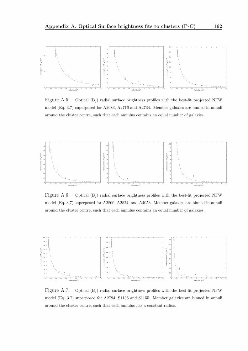
Appendix A. Optical Surface brightness fits to clusters (P-C) 162
Figure A.5: Optical (Bj) radial surface brightness profiles with the best-fit projected NFW
model (Eq. 3.7) superposed for A2683, A2716 and A2734. Member galaxies are binned in annuli
around the cluster centre, such that each annulus contains an equal number of galaxies.
Figure A.6: Optical (Bj) radial surface brightness profiles with the best-fit projected NFW
model (Eq. 3.7) superposed for A2800, A2824, and A4053. Member galaxies are binned in annuli
around the cluster centre, such that each annulus contains an equal number of galaxies.
Figure A.7: Optical (Bj) radial surface brightness profiles with the best-fit projected NFW
model (Eq. 3.7) superposed for A2794, S1136 and S1155. Member galaxies are binned in annuli
around the cluster centre, such that each annulus has a constant radius.

Appendix B
Optical Surface brightness fits to
clusters in the
Horologium-Reticulum
supercluster
In section 3.2.1 we fitted the Navarro Frenk White (NFW) X-ray surface brightness
model to optical surface brightness profiles of clusters of galaxies in superclusters,
using SuperCOSMOS data (UK Schmidt blue (Bj)). This enables us to obtain an
estimate of the virial mass of each of the clusters. This appendix contains plots of the
surface brightness profiles of the clusters of the Horologium-Reticulum supercluster
and the best fit line of the NFW model to the curves.
Figure B.1: Optical (Bj) radial surface brightness profiles with the best-fit projected NFW
model (Eq. 3.7) superposed for A2988, A3004 and A3009. Member galaxies are binned in annuli
around the cluster centre, such that each annulus has a constant number of galaxies.
163

Appendix B. Optical Surface brightness fits to clusters (H-R) 164
Figure B.2: Optical (Bj) radial surface brightness profiles with the best-fit projected NFW
model (Eq. 3.7) superposed for A3074, A3078 and A3089. Member galaxies are binned in annuli
around the cluster centre, such that each annulus has a constant number of galaxies.
Figure B.3: Optical (Bj) radial surface brightness profiles with the best-fit projected NFW
model (Eq. 3.7) superposed for A3093, A3098 and A3100. Member galaxies are binned in annuli
around the cluster centre, such that each annulus has a constant number of galaxies.
Figure B.4: Optical (Bj) radial surface brightness profiles with the best-fit projected NFW
model (Eq. 3.7) superposed for A3104, A3106 and A3109. Member galaxies are binned in annuli
around the cluster centre, such that each annulus has a constant number of galaxies.

Appendix B. Optical Surface brightness fits to clusters (H-R) 165
Figure B.5: Optical (Bj) radial surface brightness profiles with the best-fit projected NFW
model (Eq. 3.7) superposed for A3110, A3111 and A3112. Member galaxies are binned in annuli
around the cluster centre, such that each annulus has a constant number of galaxies.
Figure B.6: Optical (Bj) radial surface brightness profiles with the best-fit projected NFW
model (Eq. 3.7) superposed for A3116, A3120 and A3122. Member galaxies are binned in annuli
around the cluster centre, such that each annulus has a constant number of galaxies.
Figure B.7: Optical (Bj) radial surface brightness profiles with the best-fit projected NFW
model (Eq. 3.7) superposed for A3123, A3125 and A3128. Member galaxies are binned in annuli
around the cluster centre, such that each annulus has a constant number of galaxies.

Appendix B. Optical Surface brightness fits to clusters (H-R) 166
Figure B.8: Optical (Bj) radial surface brightness profiles with the best-fit projected NFW
model (Eq. 3.7) superposed for A3133, A3135 and A3140. Member galaxies are binned in annuli
around the cluster centre, such that each annulus has a constant number of galaxies.
Figure B.9: Optical (Bj) radial surface brightness profiles with the best-fit projected NFW
model (Eq. 3.7) superposed for A3145, A3158 and A3164. Member galaxies are binned in annuli
around the cluster centre, such that each annulus has a constant number of galaxies.
Figure B.10: Optical (Bj) radial surface brightness profiles with the best-fit projected NFW
model (Eq. 3.7) superposed for A3202, A3225 and A3266. Member galaxies are binned in annuli
around the cluster centre, such that each annulus has a constant number of galaxies.

Appendix B. Optical Surface brightness fits to clusters (H-R) 167
Figure B.11: Optical (Bj) radial surface brightness profiles with the best-fit projected NFW
model (Eq. 3.7) superposed for A3312. Member galaxies are binned in annuli around the cluster
centre, such that each annulus has a constant number of galaxies.

Appendix C
Optical Surface brightness fits to
clusters in the Shapley
supercluster
In section 3.2.1 we fitted the Navarro Frenk White (NFW) X-ray surface brightness
model to optical surface brightness profiles of clusters of galaxies in superclusters,
using SuperCOSMOS data (UK Schmidt blue (Bj)). This enables us to obtain an
estimate of the virial mass of each of the clusters. This appendix contains plots of
the surface brightness profiles of the clusters of the Shapley supercluster and the
best fit line of the NFW model to the curves.
Figure C.1: Optical (Bj) radial surface brightness profiles with the best-fit projected NFW
model (Eq. 3.7) superposed for A1631, A1644 and A1709. Member galaxies are binned in annuli
around the cluster centre, such that each annulus has a onstant radius.
168

Appendix C. Optical Surface brightness fits to clusters (S) 169
Figure C.2: Optical (Bj) radial surface brightness profiles with the best-fit projected NFW
model (Eq. 3.7) superposed for A1736, A3528N and A3528S. Member galaxies are binned in annuli
around the cluster centre, such that each annulus has a onstant radius.
Figure C.3: Optical (Bj) radial surface brightness profiles with the best-fit projected NFW
model (Eq. 3.7) superposed for A3530, A3532 and A3546. Member galaxies are binned in annuli
around the cluster centre, such that each annulus has a onstant radius.
Figure C.4: Optical (Bj) radial surface brightness profiles with the best-fit projected NFW
model (Eq. 3.7) superposed for A3552, A3555 and A3556. Member galaxies are binned in annuli
around the cluster centre, such that each annulus has a costant number of galxies in it.

Appendix C. Optical Surface brightness fits to clusters (S) 170
Figure C.5: Optical (Bj) radial surface brightness profiles with the best-fit projected NFW
model (Eq. 3.7) superposed for A3558, A3559 and A3560. Member galaxies are binned in annuli
around the cluster centre, such that each annulus has a constant number of galaxies.
Figure C.6: Optical (Bj) radial surface brightness profiles with the best-fit projected NFW
model (Eq. 3.7) superposed for A3562, A3564 and A3566. Member galaxies are binned in annuli
around the cluster centre, such that each annulus has a constant number of galaxies.
Figure C.7: Optical (Bj) radial surface brightness profiles with the best-fit projected NFW
model (Eq. 3.7) superposed for A3568, A3570 and A3571. Member galaxies are binned in annuli
around the cluster centre, such that each annulus has a constant number of galaxies.

Appendix C. Optical Surface brightness fits to clusters (S) 171
Figure C.8: Optical (Bj) radial surface brightness profiles with the best-fit projected NFW
model (Eq. 3.7) superposed for A3575, A3577 and A3578. Member galaxies are binned in annuli
around the cluster centre, such that each annulus has a constant number of galaxies.
Figure C.9: Optical (Bj) radial surface brightness profiles with the best-fit projected NFW
model (Eq. 3.7) superposed for SC1327 and SC1329. Member galaxies are binned in annuli around
the cluster centre, such that each annulus has a constant number of galaxies.

Appendix D
X-ray analysis of the Pisces-Cetus
supercluster
D.1 X-Ray observations
For the clusters that form the Pisces-Cetus supercluster (see §3.1.1), relevant X-ray
observations were taken from the data archives of the respective observatories, via
the High Energy Astrophysics Science Archive Research Center (HEASARC). The
X-ray observations were used to confirm the presence and location of the cluster,
whenever possible and determine the centre of the cluster. Where X-ray observa-
tions were available from multiple sources, ROSAT PSPC pointed observations were
preferentially used. If these were not available, ROSAT All-Sky Survey data (short
PSPC observations) or Einstein data were used.
D.1.1 ROSAT archival pointed observations
Where archival data were available for a cluster, reduction was performed using
the Asterix software package (http://www.sr.bham.ac.uk/asterix-docs). The initial
data were background subtracted, using backgrounds with point sources extracted.
The background was then flattened and used to estimate vignetting and the image
adaptively smoothed using asmooth. An estimate of the variance was found using
smooth on the largest Gaussian used in asmooth, and then this variance array
172

D.1. X-Ray observations 173
used to form a background error map. The smoothed image was then background
subtracted and divided by the background standard deviation (σ) map, to get the
number of σ above the background map. This does mean that the significance of
contours in the less heavily smoothed regions is actually an over-estimate of the
significance. The contours were then overlaid on to an optical DSS image. Contour
levels are at 5 10 20 40 ... σ above the background. The overlays for the clusters
with pointed ROSAT data can be seen in Fig. D.1.
D.1.2 Rosat all-sky Survey and Einstein IPC observations
For the clusters for which pointed X-ray observations were not available in the
archives, the ROSAT all-sky (RASS) data were inspected. If an inspection by eye
of the image, reconstructed from the event map in the energy range of 0.1-2.4 kev,
showed an extended X-ray source in the vicinity of the cluster coordinates, an X-ray
contour overlay was created using the GAIA software package. The X-ray data was
convolved with an elliptical Gaussian function and overlayed on a 20 arcminute DSS
image of centred on the cluster centre. The contour levels were linear, and chosen
to obtain a sensible contour image. The overlays for the clusters with RASS data
can be seen in Fig. D.1. A similar method to the above was used for Einstein IPC
data, contour overlays obtained and these can also be found in Fig. D.1.
D.1.3 The LX–σ relation
Theory
If it is assumed that hot gas traces the gravitating mass profile and radiates most
of its energy through bremsstrahlung radiation then,
Lx ∝ f 2gasT
2, (D.1.1)
(Ponman, Cannon, & Navarro, 1999) where fgas is the gas fraction or the ratio of the
gas to the total mass and T is the X-ray temperature. In the case of self similarity,
the gas fraction is assumed to be constant. Thus the relation becomes,
Lx ∝ T 2, (D.1.2)
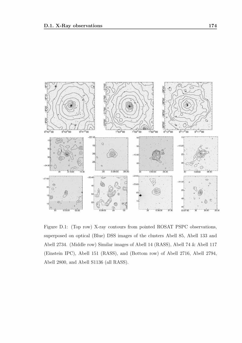
D.1. X-Ray observations 174
Figure D.1: (Top row) X-ray contours from pointed ROSAT PSPC observations,
superposed on optical (Blue) DSS images of the clusters Abell 85, Abell 133 and
Abell 2734. (Middle row) Similar images of Abell 14 (RASS), Abell 74 & Abell 117
(Einstein IPC), Abell 151 (RASS), and (Bottom row) of Abell 2716, Abell 2794,
Abell 2800, and Abell S1136 (all RASS).

D.1. X-Ray observations 175
If the virial theorem holds it follows that
σ2clus ∝
M
Rv, (D.1.3)
where σclus is the line of sight velocity dispersion, M is the mass of the cluster and
Rv is the virial radius. Hence,
σclus ∝ T 0.5, (D.1.4)
This gives rise to,
Lx ∝ σ4clus, (D.1.5)
Therefore, we would expect a gradient of 4 to the log Lx–log σ relation of our
clusters if the above assumptions hold.
D.1.4 Pisces-Cetus supercluster results
X-ray luminosities (Lx) for the individual clusters from the literature (See Table 3.1)
were converted into values of Lx in the bolometric energy range and normalised
for the Hubble constant used. The conversion was performed in PIMMS using a
Raymond-Smith model with a temperature estimated from the velocity dispersion-
temperature relation of Osmond & Ponman (2004) and a suitable H I Column Den-
sity using the HESEARC tools (http://heasarc.gsfc.nasa.gov/cgi-bin/Tools/w3nh/
w3nh.pl).
The X-ray luminosity and velocity dispersion for those of our clusters which have
both values are plotted in Fig.D.2. The line of best fit for our data gives log Lx =
6.67 log σ+24.84. We compare our results with those of Wu & Xue (1999), who used
a sample of 156 clusters from literature and obtained the relation, Lx = 10−14.57σ5.24.
For groups, Osmond & Ponman (2004) used ROSAT data for a sample of 60 groups
and obtained the relation, log Lx = 3.1 log σ−2 log(h)+34.27. However, Mulchaey &
Zabludoff (1998) found the relation log Lx = 4.29 log σ−2 log(h)+31.61 for a sample
of 12 groups with ROSAT data. These three relations are plotted for comparison
with our own in Fig. D.2 along with the data points of Osmond & Ponman (2004).
A Kolmogorov-Smirnov (KS) test was performed to find the significance of the
differences between each of the above relations and our own. It was found that the

D.1. X-Ray observations 176
Figure D.2: The relationship between Lx and σ for clusters in the Pisces-Cetus supercluster,
with available X-ray data. Cross symbols are our cluster data points while the open circle symbols
are the points for (Osmond & Ponman, 2004) for groups. Solid= best fit to the data points, dot-
dash=(Wu & Xue, 1999), dashed=(Mulchaey & Zabludoff, 1998), dash-dot-dot-dot=(Osmond &
Ponman, 2004) All values of Lx are in the bolometric energy range
probability that the Mulchaey & Zabludoff (1998) relation was drawn from the same
Lx–σ distribution as our own relation is 21.8 %. However, the relation of (Osmond
& Ponman, 2004) was found to have only a 1.8 % probability of being drawn from
the same Lx–σ distribution as our relation. The relatively low probability for the
Osmond & Ponman (2004) relation implies a possible steepening of the LX − σ
relation for clusters. This is in agreement with the results of Xue & Wu (2000) who
also found a steepening for the cluster relation.
The relation of Wu & Xue (1999) was found to have a 54.2% probability of being
drawn from the same distribution as our own relation showing a fair agreement
between the two. This would suggest little difference in the LX–σ relation of clusters
inside and out of a supercluster.
Discussion
From Eq.D.1.5, we would expect a gradient of 4 to the Lx–σ relation of our clusters.
However, our line of best fit is seen to have a steeper gradient of 5.33. This would be
consistent with the presence of pre-heating of the Intergalactic Medium, which could

D.1. X-Ray observations 177
systematically reduce the luminosity of the clusters, with a greater effect on the lower
mass clusters. A possible mechanism for the pre-heating would be the shocking of
the intergalactic medium during the formation of the large scale filaments, present
in the supercluster region, as suggested by Cen & Ostriker (1999).
Our results also show that clusters in the Pisces-Cetus supercluster have a steeper
Lx–σ relation than for groups not in a supercluster. However, there is no signifi-
cant difference in the relation for clusters that are in the Pisces-Cetus supercluster
and clusters which are not in a superluster. The flattening of the Lx–σ relation
for groups has been covered extensively in papers such as dell’Antonio, Geller, &
Fabricant (1994); Ponman et al. (1996); Xue & Wu (2000). Ponman et al. (1996)
find that their flattening of their Lx–σ relation for groups is not statistically signifi-
cant and attribute the flattening seen in dell’Antonio, Geller, & Fabricant (1994) to
the additional X-ray emission of individual galaxies, which had not been removed.
As the contribution of the individual galaxies to the group emission has not been
removed for all of our data points taken from the literature, this may be the reason
for our flattening of the Lx–σ relation for groups.
In addition the method of conversion to bolometric luminosities, based on an
uncertain temperature estimate, also reduces the validity of the comparison. Due to
the lack of a measured temperature for some clusters estimates were found using the
velocity dispersion-temperature relation of Osmond & Ponman (2004). Therefore,
the X-ray luminosities derived from these estimates are slightly dependent on the
velocity dispersion for the cluster. We therefore decided not to include this analysis
in our published paper, but include it in this dissertation as evidence of substantial
exploratory work undertaken in course of this investigation.

Appendix E
The 2dFGRS “clean sample” of
filaments
In section 5.3.1 we describe the 52 filaments that make up the 2dFGRS “clean
sample” (see Table 5.2). This appendix contains plots of the spatial distribution of
the galaxies that form each of the filaments in the “clean sample” and a plot of the
mean η and mean percentage of passive galaxies as a function of distance from the
nearest cluster for the filament galaxies.
Figure E.1: Galaxy position, mean η and mean percentage of passive galaxies in the filaments
joining the clusters: APMCC 0094 and EDCC 0457. Cluster galaxies as defined in §5.3.1 are shown
in red.
178
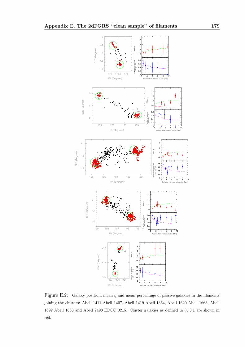
Appendix E. The 2dFGRS “clean sample” of filaments 179
Figure E.2: Galaxy position, mean η and mean percentage of passive galaxies in the filaments
joining the clusters: Abell 1411 Abell 1407, Abell 1419 Abell 1364, Abell 1620 Abell 1663, Abell
1692 Abell 1663 and Abell 2493 EDCC 0215. Cluster galaxies as defined in §5.3.1 are shown in
red.

Appendix E. The 2dFGRS “clean sample” of filaments 180
Figure E.3: Galaxy position, mean η and mean percentage of passive galaxies in the filaments
joining the clusters: Abell 2553 EDCC 0275, Abell 2601 Abell 4009, Abell 2734 EDCC 0445, Abell
2741 APMCC 0039 and Abell 2741 APMCC 0051. Cluster galaxies as defined in §5.3.1 are shown
in red.

Appendix E. The 2dFGRS “clean sample” of filaments 181
Figure E.4: Galaxy position, mean η and mean percentage of passive galaxies in the filaments
joining the clusters: Abell 2780 APMCC 0039 Abell 2814 Abell 2829, Abell 2829 Abell 0118, Abell
2829 EDCC 0511 and Abell 2878 EDCC 0511. Cluster galaxies as defined in §5.3.1 are shown in
red.

Appendix E. The 2dFGRS “clean sample” of filaments 182
Figure E.5: Galaxy position, mean η and mean percentage of passive galaxies in the filaments
joining the clusters: Abell 2915 EDCC 0581 Abell 2943 APMCC 0222, Abell 2961 APMCC 0245,
Abell 2967 Abell 2972 and Abell 2981 Abell 2999. Cluster galaxies as defined in §5.3.1 are shown
in red.

Appendix E. The 2dFGRS “clean sample” of filaments 183
Figure E.6: Galaxy position, mean η and mean percentage of passive galaxies in the filaments
joining the clusters: Abell 3980 EDCC 0268, EDCC 0217 EDCC 0202, EDCC 0365 Abell S1155,
EDCC 0445 APMCC 0094 and EDCC 0457 EDCC 0445. Cluster galaxies as defined in §5.3.1 are
shown in red.

Appendix E. The 2dFGRS “clean sample” of filaments 184
Figure E.7: Galaxy position, mean η and mean percentage of passive galaxies in the filaments
joining the clusters: EDCC 0465 Abell 2780, EDCC 0465 Abell 2814, EDCC 0517 EDCC 0511,
Abell S0333 Abell 3094 and EDCC 0119 Abell 3837. Cluster galaxies as defined in §5.3.1 are shown
in red.

Appendix E. The 2dFGRS “clean sample” of filaments 185
Figure E.8: Galaxy position, mean η and mean percentage of passive galaxies in the filaments
joining the clusters: EDCC 0057 Abell 3837, EDCC 0057 APMCC 0721, Abell 3878 Abell 3892,
EDCC 0230 APMCC 0827 and APMCC 0827 Abell 3892. Cluster galaxies as defined in §5.3.1 are
shown in red.

Appendix E. The 2dFGRS “clean sample” of filaments 186
Figure E.9: Galaxy position, mean η and mean percentage of passive galaxies in the filaments
joining the clusters: EDCC 0128 Abell 3880, Abell 3959 APMCC 0853, Abell S1075 APMCC 0167,
EDCC 0457 Abell 2794, EDCC 0492 Abell 2804. Cluster galaxies as defined in §5.3.1 are shown
in red.

Appendix E. The 2dFGRS “clean sample” of filaments 187
Figure E.10: Galaxy position, mean η and mean percentage of passive galaxies in the filaments
joining the clusters: EDCC 0202 EDCCC 0187, EDCC 0187 APMCC 0810, EDCC 0317 APMCC
4011, EDCC 0323 APMCC 4012 and Abell 3854 Abell 3844. Cluster galaxies as defined in §5.3.1
are shown in red.

Appendix E. The 2dFGRS “clean sample” of filaments 188
Figure E.11: Galaxy position, mean η and mean percentage of passive galaxies in the filaments
joining the clusters: Abell S1064 EDCCC 0153, Abell 2967 EDCCC 2981, EDCC 0239 APMCC
0853, EDCC 0248 Abell 3959 and APMCC 0167 Abell S0160. Cluster galaxies as defined in §5.3.1
are shown in red.

Appendix E. The 2dFGRS “clean sample” of filaments 189
Figure E.12: Galaxy position, mean η and mean percentage of passive galaxies in the filaments
joining the clusters: APMCC 0869 and APMCC 0840. Cluster galaxies as defined in §5.3.1 are
shown in red.