DI

SC

US

SI

ON

P

AP

ER

S

ER

IE

S

Forschungsinstitut zur Zukunft der ArbeitInstitute for the Study of Labor

The Pros and Cons of Sick Pay Schemes: A Method to Test for Contagious Presenteeism and Shirking Behavior

IZA DP No. 8850

February 2015

Stefan PichlerNicolas R. Ziebarth

The Pros and Cons of Sick Pay Schemes:

A Method to Test for Contagious Presenteeism and Shirking Behavior

Stefan Pichler ETH Zurich, KOF Swiss Economic Institute

Nicolas R. Ziebarth

Cornell University and IZA

Discussion Paper No. 8850 February 2015

IZA

P.O. Box 7240 53072 Bonn

Germany

Phone: +49-228-3894-0 Fax: +49-228-3894-180

E-mail: iza@iza.org

Any opinions expressed here are those of the author(s) and not those of IZA. Research published in this series may include views on policy, but the institute itself takes no institutional policy positions. The IZA research network is committed to the IZA Guiding Principles of Research Integrity. The Institute for the Study of Labor (IZA) in Bonn is a local and virtual international research center and a place of communication between science, politics and business. IZA is an independent nonprofit organization supported by Deutsche Post Foundation. The center is associated with the University of Bonn and offers a stimulating research environment through its international network, workshops and conferences, data service, project support, research visits and doctoral program. IZA engages in (i) original and internationally competitive research in all fields of labor economics, (ii) development of policy concepts, and (iii) dissemination of research results and concepts to the interested public. IZA Discussion Papers often represent preliminary work and are circulated to encourage discussion. Citation of such a paper should account for its provisional character. A revised version may be available directly from the author.

IZA Discussion Paper No. 8850 February 2015

ABSTRACT

The Pros and Cons of Sick Pay Schemes: A Method to Test for Contagious Presenteeism and Shirking Behavior*

This paper proposes a test for the existence and the degree of contagious presenteeism and negative externalities in sickness insurance schemes. First, we theoretically decompose moral hazard into shirking and contagious presenteeism behavior. Then we derive testable conditions for reduced shirking, increased presenteeism, and the level of overall moral hazard when benefits are cut. We implement the test empirically exploiting German sick pay reforms and administrative industry-level data on certified sick leave by diagnoses. The labor supply adjustment for contagious diseases is significantly smaller than for non-contagious diseases, providing evidence for contagious presenteeism and negative externalities which arise in form of infections. JEL Classification: I12, I13, I18, J22, J28, J32 Keywords: sickness insurance, sick pay, presenteeism, contagious diseases, infections,

negative externalities, shirking Corresponding author: Nicolas R. Ziebarth Cornell University Department of Policy Analysis and Management (PAM) 106 Martha Van Rensselaer Hall Ithaca, NY 14850 USA E-mail: nrz2@cornell.edu

* We would like to thank Davide Dragone, Laszlo Goerke, Martin Karlsson, Sean Nicholson, and Sarah Prenovitz for excellent comments and suggestions. We also thank participants in research seminars at Cornell University (PAM), the University of Linz (Economics Department), the Berlin Network of Labor Market Researchers (BeNA), and at the Centre for Research in Active Labour Market Policy Effects (CAFE) Workshop at Aarhus University for their helpful comments and suggestions. In particular we would like to thank Eric Maroney and Philip Susser for excellence in editing this paper. We or our employers have no relevant or material financial interests that relate to the research described in this paper. We take responsibility for all remaining errors in and shortcomings of the paper.

“Send me a bill that gives every worker in America the opportunity to earn seven daysof paid sick leave. It’s the right thing to do. It’s the right thing to do.”

Barack Obamain his State of the Union Address (January 20, 2015)

“I think the Republicans would be smart to get behind it.”Bill O’Reilly

in The O’Reilly Factor – Fox News (January 21, 2015)

1 Introduction

One major economic justification for publicly provided access to paid sick leave is “presen-

teeism” and negative externalities in case of contagious diseases. When workers lack access

to paid sick leave, they may go to work despite being sick. This situation is referred to

as “presenteeism.” Particularly in professions with direct customer contact, presenteeism

in case of contagious diseases unambiguously leads to negative externalities and infection

spillovers to co-workers and customers. Given the low vaccination rates of around 40% in

the US and 10% to 30% in the EU (Blank et al., 2009; Centers for Disease Control and Pre-

vention, 2014a), workplace presenteeism is one important channel through which infectious

diseases spread. After the first occurrence of flu sickness symptoms, humans are conta-

gious for 5 to 7 days (Centers for Disease Control and Prevention, 2014b). Over-the-counter

(OTC) drugs that suppress symptoms but not contagiousness promote the spread of dis-

ease in cases of presenteeism and non-insured workplace absenteeism (Earn et al., 2014).

Worldwide, seasonal influenza epidemics alone lead to 3 to 5 million severe illnesses and

an estimated 250,000 to 500,000 deaths; in the US, flu-associated annual deaths range from

3,000 to 49,000 (World Health Organization, 2014; Centers for Disease Control and Preven-

tion, 2014b).

Opponents of universal paid sick leave point to the fact that such social insurance sys-

tems would encourage shirking behavior and reduce labor supply. Moreover, forcing em-

ployers to provide sick pay via mandates or new taxes would dampen job creation and hurt

employment. A last argument against state regulated paid sick leave is that the private

market would ensure that employers voluntarily provide such fringe benefits if such fringe

benefits were truly optimal.

1

Historically, paid sick leave was actually one of the first social insurance pillars world-

wide: This policy was included in the first federal health insurance legislation. Under Otto

van Bismarck, the Sickness Insurance Law of 1883 introduced social health insurance which

included 13(!) weeks of paid sick leave along with coverage for medical bills. The costs

associated with paid sick leave initially made up more than half of all program costs, given

the limited availability of expensive medical treatments in the 19th century (Busse and Ries-

berg, 2004). Other European countries followed quickly and, today, virtually every Euro-

pean country has some form of universal access to paid sick leave—with varying degrees

of generosity. The US is the only industrialized country worldwide without universal ac-

cess to paid sick leave (Heymann et al., 2009). 49% of American employees have no ac-

cess to sick pay, particularly low-income and service sector workers (Lovell, 2003; Boots

et al., 2009). However, in the US, support for paid sick leave has grown substantially in the

last decade: Several sick leave schemes were implemented in Seattle, Washington D.C., San

Francisco, and most recently New York City. Connecticut was the first state to introduce a

sick leave scheme (for service sector workers in non-small businesses) in 2012. Reintroduced

in Congress in March 2013, the Healthy Families Act foresees the introduction of universal

paid sick leave for up to seven days per employee and year at the federal level .

As outlined above, the economic legitimation for paid sick leave hinges crucially on

the existence of negative externalities and presenteeism with regard to contagious diseases.

However, empirically proving the existence of presenteeism in cases of contagious diseases

is extremely difficult. Several empirical papers have evaluated the causal effects of cuts in

sick pay, and found that employees adjust their labor supply in response to such cuts (Jo-

hansson and Palme, 1996, 2005; Ziebarth and Karlsson, 2010; De Paola et al., 2014; Ziebarth

and Karlsson, 2014; Dale-Olsen, 2014; Fevang et al., 2014).1 Traditionally, behavioral ad-

justments to varying levels of insurance generosity is labeled moral hazard in economics

(Pauly, 1974, 1983; Arnott and Stiglitz, 1991; Nyman, 1999; Newhouse, 2006; Felder, 2008;

1Other papers in the literature on sickness absence looked at and decomposed general determinants(Barmby et al., 1994; Markussen et al., 2011), investigated the impact of probation periods (Riphahn, 2004;Ichino and Riphahn, 2005), culture (Ichino and Maggi, 2000), gender (Ichino and Moretti, 2009), income taxes(Dale-Olsen, 2013), and unemployment (Askildsen et al., 2005; Nordberg and Røed, 2009; Pichler, 2014). Thereis also research on the impact of sickness on earnings (Sandy and Elliott, 2005; Markussen, 2012).

2

Bhattacharya and Packalen, 2012). However, in case of sick leave, being able to disentangle

shirking behavior from presenteeism is crucial in order to derive valid policy conclusions.

The main objective of this paper is to develop an approach to test for the existence of

shirking, contagious presenteeism and associated negative externalities in workplace set-

tings with sickness insurance coverage. This paper is the first in the economic literature

to define and test for the existence of contagious presenteeism. The first part of the paper

develops an economic model that decomposes moral hazard into shirking and contagious

presenteeism. According to this theoretical framework, the negative externalities can be

quantified by assessing changes in infections after changes in sick pay. The model pre-

dicts that changes in sick pay induce changes in the two undesired behaviors that work

in opposite directions: shirking and contagious presenteeism. We explicitly refrain from a

normative welfare analysis which would require to weight these two phenomena, depend-

ing on societal preferences. We rather provide a positive analysis and the first approach to

theoretically define and empirically measure these countervailing effects.

The second part of the paper exploits two German policy reforms which varied the level

of sick pay. Using administrative data aggregated at the industry level and differences in

industry-specific sick pay regulations, we show that sick pay cuts from 100 to 80% of fore-

gone wages reduced the sickness rate by about 20% on average. This is in line with the stan-

dard predictions of our model and the previous literature (Johansson and Palme, 1996, 2005;

Ziebarth and Karlsson, 2010; Puhani and Sonderhof, 2010; De Paola et al., 2014; Ziebarth and

Karlsson, 2014; Fevang et al., 2014). Next, and more importantly, we are able to analyze the

labor supply effects separately by certified disease categories. In line with the theoretical

model implications, we find disproportionately large labor supply adjustments for muscu-

loskeletal diseases. Meanwhile, the sickness rate of infectious diseases did not decrease by

the same proportions. This difference can be explained by additional infections that increase

sick leave rates and compensate for reductions due to lower sick pay. Thus, when mandated

sick pay is lowered, policymakers have to consider the trade-off between (i) the short-run

effect of a reduction in shirking vs. (ii) an increase in contagious presenteeism leading to

(iii) a higher infection rate and more relapses in the medium-run.

3

Obviously, this paper is close in spirit to papers that estimate causal labor supply effects

of changes in sick pay levels (e.g. Johansson and Palme, 1996, 2002, 2005; Ziebarth, 2013;

Ziebarth and Karlsson, 2010, 2014). In particular, it extends the small economic literature on

presenteeism at the workplace (Aronsson et al., 2000; Chatterji and Tilley, 2002; Brown and

Sessions, 2004; Pauly et al., 2008; Barmby and Larguem, 2009; Markussen et al., 2012; Pichler,

2014). With one exception, none of the empirical studies on presenteeism just cited identi-

fies or intends to identify causal effects of sick leave schemes on presenteeism. Markussen

et al. (2012) studies the impact of partial absence certificates on presenteeism but defines

presenteeism very broadly—as a reduction in sick leave when activation requirements be-

come tighter. Pauly et al. (2008) ask 800 US managers about their view on employee pre-

senteeism with (a) chronic and (b) acute diseases—with respect to firm costs and separately

by occupation and type of work. Pichler (2014) provides evidence for the hypothesis that

presenteeism is procyclical due to a higher workload during economic booms. A paper that

is similar to ours is Barmby and Larguem (2009). They exploit daily absence data from a sin-

gle employer and estimate absence determinants as well as transmission rates of contagious

diseases, linking the estimation approach nicely to an economic model of absence behavior.

Finally, this paper also adds to the literature on the determinants and consequences of

epidemics and vaccinations (cf. Mullahy, 1999; Bruine de Bruin et al., 2011; Uscher-Pines

et al., 2011). For example, Maurer (2009) models supply and demand side factors of in-

fluenza immunization, whereas Karlsson et al. (2014) empirically assess the impact of the

1918 Spanish Flu on economic performance in Sweden.

The first part of the paper theoretically defines and decomposes moral hazard into shirk-

ing and contagious presenteeism behavior in case of sick leave. The empirical application

of our proposed test exploits variation in federal employer mandates in combination with

industry-specific collective bargaining regulations. Note that the theory and empirical sec-

tions do not hinge on whether the sick pay scheme is mandated by the government or not,

and this paper’s main objective is not to study the welfare effects of employer mandates,

but rather to generally decompose moral hazard in the context of employer-provided sick

pay schemes. Although related and sometimes combined in laws, sick pay schemes differ

4

crucially from maternity leave schemes due to (i) the negative externalities induced by con-

tagious presenteeism in combination with (ii) information asymmetries between employers

and employees about the type and extend of the employee’s disease. Several important pa-

pers study the labor market effects of mandated maternity and family leave (Gruber, 1994;

Ruhm, 1998; Waldfogel, 1998; Rossin-Slater et al., 2013; Thomas, 2015).

The next section discusses our economic model and derives testable conditions under

presenteeism and contagious diseases. Section 3 explains the German sick leave system and

the policy reforms. Section 4 discusses the data, the variables generated, and the empirical

approach. In the final two sections, we present the empirical results and conclude.

2 A Method to Identify Contagious Presenteeism and

Negative Externalities

2.1 Modeling Shirking and Presenteeism

We extend and build upon a mix of standard leisure-work models to theoretically study

the absence behavior of workers (cf. Brown, 1994; Barmby et al., 1994; Brown and Sessions,

1996). While there might be additional arguments for or against the provision of sick pay,

our theoretical model below focuses on employee shirking and presenteeism behavior, the

associated infections, and the consequential trade-off.2 Since we construct a model of in-

dividual behavior we omit the i subscript in order to simplify notation. We specify the

individual utility function as:

ut = (1− σt)ct + σtlt, with σt ∈ [0, 1] , (1)

2In particular, we abstain from modeling the employer’s side and effects on the firm level. This couldinclude employer signaling (or adverse selection) effects, peer effects, or discrimination against identifiableunhealthy workers (e.g. obese workers). We also abstain from analyzing general equilibrium labor marketeffects.

5

where ut represents the utility of a worker at time t, ct stands for consumption and lt for

leisure. The current sickness level is σt, with larger values of σt representing a higher degree

of sickness. This parameter is private information of the worker and unknown by the firm.

In time periods with high levels of σt, i.e., when the worker is very sick, utility is mostly

drawn from leisure or recuperation time rather than consumption. On the other hand, if the

sickness level is relatively low, the worker attaches more weight to consumption as opposed

to leisure.3

With h defining hours of contracted work, T the total amount of time available—and

assuming that workers are not saving, but consuming their entire income from work wt

or sick pay st—one can write the indifference condition between working and (sickness)

absence formally as:

(1− σt)st + σtT = (1− σt)wt + σt(T − h). (2)

In most countries sick pay is not a flat monetary amount but rather a replacement rate

of the current wage. Hence we substitute sick pay with st = αtwt in the equation above

(with αt ∈ [0, 1]).4 Moreover, workers are paid based on their average productivity and,

approximating reality, we assume rigid wages and thus a time invariant wage level w. We

can then calculate the indifference point σ∗(αt) for a given replacement rate αt:

σ∗(αt) =(1− αt)w

(1− αt)w + h. (3)

Hence if σt > σ∗(αt) workers will be absent, while they will be present if σt < σ∗(αt). The

latter can be thought of the “normal” state under which the great majority, 80 to 90% of all

workers, fall every day. The value of σ∗(αt) where workers are indifferent solely depends on

3While our model focuses on sickness and sickness absence, in principle a high σt only indicates a temporarypreference for leisure. This might not necessarily be related to sickness and associated recuperation time, butalso to other factors, such as sickness of family members and recreational activities.

4Notice that the wage may also include non-monetary benefits, such as more job security. For instanceScoppa and Vuri (2014) find that workers who are absent more frequently face higher risks of dismissal. Thuseven in countries with nominally full replacement, in our model, this might translate to a replacement ratesmaller than one due to future income opportunities and other costs and benefits.

6

(i) the amount of money workers lose while on sick leave, (1− αt)w, and (ii) the contracted

amount of working hours h.

Introducing Two Types of Diseases and Negative Externalities Due to Contagious Pre-

senteeism

Next, let us assume that two types of (mutually exclusive) diseases exist: (i) contagious dis-

eases denoted by subscript c, e.g., flus and (ii) non-contagious diseases denoted by subscript

n, e.g. back pain.5 More precisely, we assume that at every point in time the worker is either

healthy σt = 0 with probability 1− q − pt,6 sick due to a non-contagious disease σt = σnt

with probability q or sick due to a contagious disease σt = σct with probability pt. In the

latter two cases the actual size of the disutility created by the sickness σt is determined by

the density function f (σ). Thus while the level of σt determines the decision of the worker

to stay at home or not, we now add an additional characteristic to this variable which deter-

mines whether the disease is contagious or not. Moreover, we assume that conditional on

being sick (σ > 0) the probabilities of disease types (pt and q) are independent of the density

of the sickness level f (σ).

As already mentioned, both the severity of the disease and the worker’s “disease type”

drawn by the worker is private information and thus we abstract away from situations when

an employer detects a worker with a contagious disease at work and sends the worker home

in order to avoid infections. This private information assumption seems reasonable given

that disease type and contagiousness are mostly unobservable and subject to very incom-

plete monitoring. In that context, consider that most infectious diseases are contagious for

days before symptoms are clearly observable. The availability and popularity of OTC drugs

suppressing disease symptoms reinforce the unobservability assumption (Earn et al., 2014).

Finally, the probability of being affected by a contagious disease pt changes over time

depending on infections in the previous period, as outlined in detail below. The probability

5In principle non-contagious diseases represent a special case of contagious diseases, where infections areequal to zero. Moreover, (diseases with) relapses can also be considered as a special case of contagious diseases,where the level of contagiousness is fairly low, as individuals “infect” only themselves.

6We assume that these probabilities are the same for all individuals considered.

7

for drawing a non-contagious diseases q on the other hand is not time varying but fixed and

thus we omit the time index t.7

Given σ∗(αt) and assuming a worker population of size 1, we can now define the sick

leave rate At as the share of individuals absent from work:

At = Act + Ant = (pt + q)1∫

σ∗(αt)

f (σ)dσ; (4)

similarly, the share of workers present is given by

Pt = (1− pt − q) + (pt + q)σ∗(αt)∫

0

f (σ)dσ. (5)

Given the replacement rate αt, a share of workers

πt(αt) = pt

σ∗(αt)∫0

f (σ)dσ (6)

is contagious but present at work. We define πt(αt) as contagious presenteeism. One eco-

nomic purpose of providing paid sick leave is to provide financial incentives such that in-

fections caused by contagious presenteeism are minimized.

As seen, the share of workers with contagious presenteeism behavior who transmit dis-

eases to their co-workers and to customers equals πt(αt). Following a standard SIS (susceptible-

infected-susceptible) endemic model,8 the transmission of diseases at the workplace de-

pends on three factors: (a) the share of contagious workers working (the infected) πt, (b)

the share of non-contagious individuals present at work (the susceptibles) St = (1− pt −

q) + qσ∗(αt)∫

0f (σ)dσ , and (c) the transmission rate of the disease which we denote with r.9

Therefore the probability of catching a contagious disease is an increasing function of these

7Notice that we abstract from any competing risks since an increase in contagious diseases does not affectthe probability of having a non-contagious diseases. While substitution might take place, we assume it is of asmall enough margin not to be considered here.

8The SIS model is the classic framework for mathematically analyzing contagious diseases and was firstdiscussed in the medical literature by Ross (1916) and Kermack and McKendrick (1927).

9It is outside the scope of this paper to model the transmission rate of contagious diseases explicitly (cf.Philipson, 2000; Barmby and Larguem, 2009; Pichler, 2014).

8

three elements pt(πt, St, r). Thus contagious workers who show up at the workplace trigger

the negative externalities that sick pay schemes intend to minimize.

Severely Sick Workers and Shirkers

If σt > σ∗(0) workers are too sick to work and would stay at home even if the replacement

rate was equal to zero and they would fully forgo their wage. The utility function in this case

approximates ut = δσtlt. This can be thought of as a state where people are either (i) lying

in bed with extremely high fever and heavy, acute, flu symptoms (as an example for a con-

tagious disease), or (ii) lying in bed with heavy disease symptoms, e.g., after chemotherapy

in case of cancer (as an example for a non-contagious disease). Empirically, one can estimate

that about 3 to 5% of all workers fall into this category on a given day.10

As sick pay is provided (αt > 0) there will be a share of workers who stay at home due to

their sick pay insurance (workers with σ∗(αt) < σt < σ∗(0)). These individuals would go to

work, if there was no sick pay. However, since they receive sick pay benefits, it is rational for

them to be absent from work. In the domain of non-contagious diseases, we refer to these

workers as shirkers. The share of shirkers at any point in time and for a given sick pay

replacement level αt equals

ω(αt) = qσ∗(0)∫

σ∗(αt)

f (σ)dσ (7)

for non-contagious diseases.

As productivity is hard to measure in most settings, we do not model work produc-

tivity explicitly. However, for non-contagious diseases, lower productivity due to sickness

mostly dominates sickness absence and zero work output. Formally, denote with δ(σ∗(0))

the sickness-related productivity losses for workers that are just indifferent between going

to work and staying at home at a replacement rate of zero. If worker utility and firm profits

have similar weights, then as long as σ∗(0)αtw > δ(σ∗(0)) work is preferred to sickness

absence. This condition compares the consumption utility from sickness benefits with the

10In Germany, on a given day, about 7% of the workforce are on sick leave (see Section 3.2).

9

productivity losses from a sick non-contagious worker. Sickness absence is preferred from

a societal point of view only if the productivity losses or consumption utility losses due to

sickness are very large. For the rest of the paper we assume that σ∗(0)αtw > δ(σ∗(0)), and

thus working is preferred to sickness absence for non-contagious diseases, as long as the

disease is not too severe σt < σ∗(0).

Finally, we define moral hazard as the sum of the fraction of shirking individuals and

the fraction of individuals exhibiting contagious presenteeism 11

ρt(αt) = ω(αt) + πt(αt). (8)

Proposition 1. Under a sick pay scheme and given the existence of contagious as well

as non-contagious diseases, there exists a fraction of contagious workers πt that engage in

presenteeism. Contagious workers who go to work induce negative externalities and infect

their co-workers and customers. Likewise, there exists a fraction of workers who shirk, ω,

while shirking behavior is determined by non-contagious diseases. Moral hazard, ρt, is the

sum of shirking and presenteeism.

In the specification above the main difference between contagious and non-contagious

diseases is that contagious diseases lead to contagious presenteeism and infections, which

increases the probability of infections. This negative externality is one of the main economic

justifications for sick pay. The extent of this negative externality depends on the level of

contagiousness of the disease. Therefore, in the context of our model, presenteeism is not

harmful per se, but rather the negative externalities generated by presenteeism.

Sick Pay Cuts and Their Impact on Moral Hazard: Intuitive and Graphical Representation

In order to simplify the analysis, we assume (without loss of generality) that sick pay in

the base year (t = 0) is high and is exogenously cut after one year in t = y1. Deriving the

indifference condition in equation (3) yields ∂σ∗(α)∂α < 0. This means that a decrease in the

11Similar to Einav et al. (2013) moral hazard is strictly speaking not a hidden action in our context, since itis perfectly observable whether the employee is present or not. It is rather hidden information that employeeshave about their personal sickness level and their type of sickness.

10

sick pay replacement rate—as induced by the first German reform in 1996—increases σ∗ and

thus more workers work, i.e., the sick leave rate decreases.

Following a sick pay cut, work attendance increases and sick leave decreases. However,

what is even more relevant is how contagious presenteeism and shirking behavior changes.

It can easily be shown that (i) shirking decreases because σ∗(αy1) > σ∗(α0). Moreover, (ii)

contagious presenteeism increases for the same reason. Thus it remains ambiguous what

happens to overall moral hazard since the first component of moral hazard, contagious pre-

senteeism, increases while the second component, shirking, decreases.

Proposition 2. Given the existence of contagious as well as non-contagious diseases,

a sick pay cut increases the share of contagious workers who engage in presenteeism and

who induce negative externalities by infecting co-workers and customers. At the same time,

a sick pay cut reduces the fraction of shirkers. A priori, the impact on moral hazard defined

as the sum of both behaviors is ambiguous.

Figure 1 shows a graphical representation of Proposition 2. Panel A depicts the situation

for non-contagious diseases. Initially the share of shirkers—indicated by the sum of the two

dark gray areas—is quite large. However, as sick pay decreases, some shirkers come to work

and the shirking rate and overall absences decrease.

In Panel B we show the situation for contagious diseases. Here all individuals that are

working exhibit contagious presenteeism. As sick pay decreases, contagious presenteeism

increases. This leads to an increase in the probability of catching a contagious disease pt,

depicted by an outward shift of the density function.

In the next step, we investigate in more detail how absence rates are affected by a sick

pay cut. Exactly the reverse pattern holds for increases in the generosity of sick pay schemes.

11

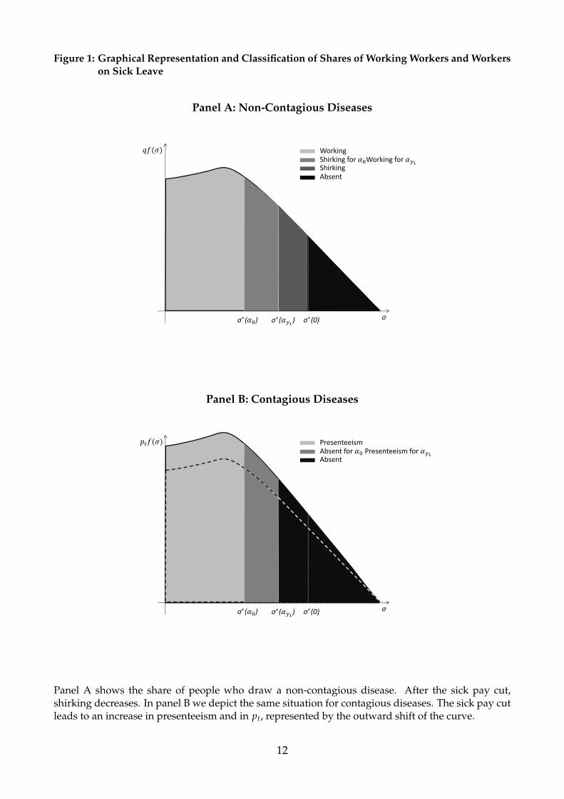
Figure 1: Graphical Representation and Classification of Shares of Working Workers and Workerson Sick Leave

Panel A: Non-Contagious Diseases

σσ∗( ) σ∗( ) σ∗(0)

WorkingShirking for Working forShirkingAbsent

Panel B: Contagious Diseases

σσ∗( ) σ∗( ) σ∗(0)

PresenteeismAbsent for Presenteeism for Absent

Panel A shows the share of people who draw a non-contagious disease. After the sick pay cut,shirking decreases. In panel B we depict the same situation for contagious diseases. The sick pay cutleads to an increase in presenteeism and in pt, represented by the outward shift of the curve.

12

Sick Pay Cuts and Their Impact on Moral Hazard: Analytical Derivation

We denote by ∆AnAn0

= βnτ the percentage change in the sick leave rate of non-contagious

diseases as the replacement rate decreases, and after τ time periods have passed; more

specifically

βnτ =1

An0

q1∫

σ∗(α0)

f (σ)dσ− q1∫

σ∗(ατ)

f (σ)dσ

=1

An0

qσ∗(ατ)∫

σ∗(α0)

f (σ)dσ

. (9)

As we are in the domain of non-contagious diseases, the reduction in absence is equal to the

reduction in shirking when sick pay decreases, and thus we can write

βnτ =1

An0(ω(α0)−ω(ατ)) . (10)

Similarly we denote by ∆AcAc0

= βcτ the percentage change of the sick leave rate of conta-

gious diseases due to a change in the replacement rate after τ time periods:

βcτ =1

Ac0

p0

1∫σ∗(α0)

f (σ)dσ− pτ

1∫σ∗(ατ)

f (σ)dσ

. (11)

This expression can be rewritten as

βcτ =1

Ac0

(π0(ατ)− π0(α0))−

(pτ − p0)

1∫σ∗(ατ)

f (σ)dσ

, (12)

where the first element corresponds to the increase in presenteeism (and corresponding de-

crease in the absence rate) due to the sick pay cut—applying the initial probability of catch-

ing a contagious disease p0. The second element corresponds to absence created by addi-

tional infections due to increased presenteeism.

As described above, infections lead to an increase in the infection rate pt. As seen in

Proposition 2, more contagious workers work after the sick pay cut. Furthermore, as more

workers work, the number of susceptibles increases as well. Both effects result in more infec-

tions. Depending on the magnitude of newly infected individuals, the increase in sickness

13

absence due to infections at least partly offsets the decrease due to additional contagious

presenteeism.

In the next step, we compare the two changes in the sick leave rate, where βcτ and βnτ

can be rewritten as:

βcτ = βnτ −1

Ac0

(pτ − p0)

1∫σ∗(ατ)

f (σ)dσ

(13)

Therefore the adjustments of shirking and presenteeism with respect to the sick pay cut

are exactly equal. Moreover, the adjustments of the two disease groups βcτ and βnτ only

differ by the share of newly infected individuals weighted by the share of individuals on

sickness leave before the sick pay cut. Thus, under the existence of contagious presenteeism,

it holds that βnτ > βcτ. Finally, notice that by definition βnτ > 0. However—for contagious

diseases—the sign of βcτ is unclear. If the disease is very contagious βcτ might become neg-

ative. Therefore the sign of βcτ remains an empirical question which can only be answered

with appropriate data.

Hypothesis 1 After a sick pay cut the absence rate for non-contagious diseases, i.e. shirk-

ing, will decrease βnτ > 0. For contagious diseases, the sign of βcτ is unclear, since absences

due to new infections might outweigh the immediate decrease in the absence rate caused

by the increase in presenteeism. Moreover, the difference βnτ − βcτ indicates the additional

absences created by infections.

Finally, we denote the overall percentage change with βτ = ∆AA0

:

βτ =1

A0

(ω(α0)−ω(ατ)) + (π0(ατ)− π0(α0))−

(pτ − p0)

1∫σ∗(ατ)

f (σ)dσ

. (14)

In the next step we analyze how these effects may be measured using data on sickness

absence, in order to quantify the reduction in shirking and the new infections due to the sick

pay cut.

14

2.2 Identifying Presenteeism Empirically

Now assume that we have empirical data on sick leave behavior and a sick leave scheme

exists. Furthermore, assume a reform has cut sick pay and we can identify different groups

of workers who were affected differently by the reform. Then we can estimate the causal

effect of the sick pay cut on the share of workers who call in sick. In the notation above,

this means that we can empirically identify the percentage change of sickness absence with

respect to the sickness cut βτ.

Moreover, assume that we could even empirically identify two different disease cate-

gories c and n and the share of employees who call in sick with certified sickness due to

contagious and non-contagious diseases. Then one could carry out a statistical test to check

if βnτ > βcτ. In other words, one could test if the sick pay induced decrease in sick leave is

larger for disease categories n as compared to c, due to the increased spread of contagious

diseases via an increase in contagious presenteeism.

Proposition 4a. Given the existence of a reform that exogenously cut sick pay and data

on differently affected employees, one can econometrically test if βτ > 0, i.e., if the labor

supply adjustment with respect to sick pay is positive and, if so, how large it is.

Proposition 4b. Given the additional existence of data for contagious and non-contagious

sick leave rates, one can estimate βnτ as well as βcτ. The size of βnτ is informative for the

relevance of shirking behavior. βcτ estimates a combination of the increase in presenteeism

and increase in infections triggered by contagious presenteeism.

Proposition 4c. Additionally, one can econometrically test if βnτ > βcτ (Hypothesis

1), i.e., whether the decrease in sick leave is larger for non-contagious than for contagious

diseases and, if yes, how large the differential is. Finally, the size of the differential represents

the existence and the degree of infections—the negative externalities induced by the lower

sick pay level.

15

3 The Sick Leave Reforms and Induced Changes in Replace-

ment Rates

3.1 The German Sick Pay Scheme and Monitoring System

Germany has one of the most generous universal sickness insurance systems in the world.

The system is predominantly based on employer mandates. In Germany, employers are

mandated to continue wage payments for up to six weeks per sickness episode. In other

words, employers have to provide 100% sick pay from the first day of a period of sickness

without benefit caps.12

In the case of illness, employees are obliged to inform their employer immediately about

both the sickness and the expected duration. From the fourth day of a sickness episode, a

doctor’s certificate is required and is usually issued for up to one week, depending on the

illness. However, employers have the right to ask for a doctor’s note from the first day of a

spell and many employee voluntarily submit doctor’s notes from the beginning of a sickness

episode.

If the sickness lasts more than six continuous weeks, the doctor needs to issue a different

certificate. From the seventh week onwards, sick pay is disbursed by the health insurers

(called “sickness funds”) and lowered to 80% of foregone gross wages for those who are

insured under Statutory Health Insurance (SHI).13

The monitoring system mainly consists of an institution called Medical Service of the

SHI. One of the original objectives of the Medical Service is to monitor sickness absence.

German social legislation codifies that the SHI has the right to call for the Medical Service

and a medical opinion to clarify any doubts about work absences. Such doubts may arise if

the insured person is short-term absent with unusual frequency or is regularly sick on Mon-

12 The entitlement is codified in the so-called Gesetz uber die Zahlung des Arbeitsentgelts an Feiertagen undim Krankheitsfall (Entgeltfortzahlungsgesetz), article 3, 4.

13 In principle, there is no limit on the frequency of sick leave spells. However, if employees fall sick againdue to the same illness after an episode of six weeks, the law explicitly states that they are only again eligiblefor employer-provided sick pay if at least six months have been passed between the two spells or twelvemonth have been passed since the beginning of the first spell. This paragraph intends to avoid substitution oflong-term spells by short-term spells.

16

days or Fridays. Similarly, if doctors certify sickness with unusual frequency, the SHI may

ask for expert advice. The employer also has the right to call for the assistance of the Medical

Service and expert advice. Expert advice is based on available medical documents, informa-

tion about the workplace, and a statement which is requested from the patient. If necessary,

the Medical Service has the right to conduct a physical examination of the patient and to cut

benefits.14 In 2012, about 2,000 full-time equivalent and independent doctors worked for

the medical service and examined 1.5 million cases of absenteeism (Medizinischer Dienst

der Krankenversicherung (MDK), 2014).

3.2 The Policy Reforms

In 1996, the total sum of employer-provided sick pay amounted to EUR 28.2 billion or 1.5%

of GDP (German Federal Statistical Office, 1998). It was though of as a tax on labor and

was attributed with unemployment rates. In addition there were speculations of a high

degree of shirking behavior. Relating the average number of sick days per year to the annual

number of hours worked per employee shows that more than 7% of the annual working time

was “lost” (Bundesverbank der Betriebskrankenkassen (BKK), 2004; Hans Bockler Stiftung,

2014). These considerations incited the German center-right government to pass a Bill to

Foster Growth and Employment which became effective on October 1, 1996.15 Panel A of

Table 1 summarizes the changes in the federal employer mandate due to this bill.

14 The wording of the laws can be found in the Social Code Book V, article 275, para. 1, 1a; article 27615 Passed on September 25, 1996 this law is the Arbeitsrechtliches Gesetz zur Forderung von Wachstum und

Beschaftigung (Arbeitsrechtliches Beschaftigungsforderungsgesetz), BGBl. I 1996 p. 1476-1479.

17

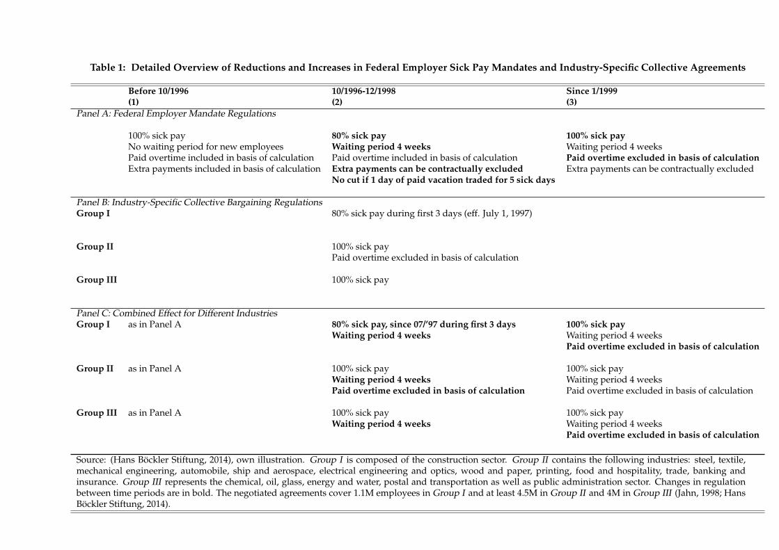
Table 1: Detailed Overview of Reductions and Increases in Federal Employer Sick Pay Mandates and Industry-Specific Collective Agreements

Before 10/1996(1)

10/1996-12/1998(2)

Since 1/1999(3)

Panel A: Federal Employer Mandate Regulations

100% sick pay 80% sick pay 100% sick payNo waiting period for new employees Waiting period 4 weeks Waiting period 4 weeksPaid overtime included in basis of calculation Paid overtime included in basis of calculation Paid overtime excluded in basis of calculationExtra payments included in basis of calculation Extra payments can be contractually excluded Extra payments can be contractually excluded

No cut if 1 day of paid vacation traded for 5 sick days

Panel B: Industry-Specific Collective Bargaining RegulationsGroup I 80% sick pay during first 3 days (eff. July 1, 1997)

Group II 100% sick payPaid overtime excluded in basis of calculation

Group III 100% sick pay

Panel C: Combined Effect for Different IndustriesGroup I as in Panel A 80% sick pay, since 07/’97 during first 3 days 100% sick pay

Waiting period 4 weeks Waiting period 4 weeksPaid overtime excluded in basis of calculation

Group II as in Panel A 100% sick pay 100% sick payWaiting period 4 weeks Waiting period 4 weeksPaid overtime excluded in basis of calculation Paid overtime excluded in basis of calculation

Group III as in Panel A 100% sick pay 100% sick payWaiting period 4 weeks Waiting period 4 weeks

Paid overtime excluded in basis of calculation

Source: (Hans Bockler Stiftung, 2014), own illustration. Group I is composed of the construction sector. Group II contains the following industries: steel, textile,mechanical engineering, automobile, ship and aerospace, electrical engineering and optics, wood and paper, printing, food and hospitality, trade, banking andinsurance. Group III represents the chemical, oil, glass, energy and water, postal and transportation as well as public administration sector. Changes in regulationbetween time periods are in bold. The negotiated agreements cover 1.1M employees in Group I and at least 4.5M in Group II and 4M in Group III (Jahn, 1998; HansBockler Stiftung, 2014).

Sick Pay Cut at the End of 1996

As seen in Table 1, the bill reduced the sick pay obligations of private sector employers from

100% to 80% of foregone wages.16 For obvious reasons, self-employed were not affected by

this change in the employer mandate.17Private sector employees on sick leave due to work

accidents were also unaffected by the bill, being explicitly excluded from the cut in sick pay.

In addition to the reduction in the level of sick pay, a four week waiting period for new

employees was introduced (Panel A of Table 1). Moreover, the bill introduced two options:

(a) The first allowed employers to contractually exclude extra payments from the basis of

calculation to which the replace rate is applied. (b) The second allowed employees to swap

one day of paid vacation for five days of sick leave, thereby avoiding the cut to 80%.18 It is

unclear to what degree these new options were applied by employees and employers. Since

we do not have any information on their relevance and also could not find explicit infor-

mation on their use in industry-specific collective agreements, henceforth, we assume that

they were either of minor relevance or were not applied systematically in specific industries

(and thus abstain from commenting on them further). A scattered application of these two

options should not significantly bias our empirical findings.

Both before and after the bill’s implementation, through mass demonstrations and strikes,

the general public and unions put pressure on employers’ associations to not apply these

less generous minimum standards. Germany is the country of origin of Bismarckian cor-

poratism, which has served as a model for several European countries. An integral part of

Bismarckian corporatism is the idea of social partnership between employers and unions

16 In addition to this bill that lowered employer-mandated sick pay, another bill cut long-term sick pay fromthe seventh week onwards from 80% to 70% of forgone gross wages. Ziebarth (2013) shows that this secondbill did not induce significant behavioral reactions among the long-term sick.

17 Figure 2 of Ziebarth and Karlsson (2010) illustrates the overall structure of affected and unaffected em-ployees in Germany. Due to political considerations and the existence of other laws, public sector employeeswere exempt from the reform. This paper solely focuses on the implementation at the industry level amongemployees who were covered by collective agreements, i.e., up to 15 million private sector employees plus upto 5 million in public administration (see Table 1). The empirical part is solely based on those employees whowere enrolled in one of the 690 (out of 960) company-specific health plans (“Betriebskrankenkassen”) (GermanFederal Statistical Office, 2014).

18 Note that this option was likely introduced to dampen potential presenteeism by low-wage employeeswho could not afford to forgo 20% of their daily wage. Those employees would not suffer a monetary loss ifthis option was drawn, but “lost” one day of paid vacation for five sick days, which is the monetary equivalentto a daily cut by 20%.

19

as well as autonomy in bargaining. As a result, unions are traditionally strong in Germany

as is the degree of collective bargaining coverage. In 1998, about 68% of all employees in

West and 50% in East Germany were covered by collective wage agreements (Hans Bockler

Stiftung, 2014).

Ongoing union pressure forced employer associations in various industries to agree,

through collective agreements, to voluntarily provide sick pay on top of the statutory reg-

ulations. Further, the question of whether employees in specific industries were entitled to

claim 100% or 80% of their salary during sickness episodes was determined by existing col-

lective agreements and their legal interpretation. Some existing agreements explicitly, but

probably coincidentally, stated that sick pay would be 100%, while others did not mention

sick pay at all. In the former case, sick pay would remain 100% despite the decrease in the

generosity of the employer mandate, while sick pay would decrease in the latter case to 80%

until a revised agreement was negotiated.

Review of Collective Agreements. Similar to Ziebarth and Karlsson (2010) and Ziebarth

and Karlsson (2014), we reviewed all collective agreements that were implemented during

the same time period of the two sick pay reforms and categorized industries. Overall, one

can distinguish three different groups and industries that implemented the following sick

leave regulations in their collective agreements on the industry level. Panel A of Table 1

shows the federal regulation, whereas Panel B provides the provisions at the industry level

and our categorization.

Group I is composed of the construction sector. The existing collective agreement cov-

ered about 1.1 million private sector workers.19 When the law was passed, this existing col-

lective agreement did not include any explicit provision on sick pay, which is why the entire

federal regulations applied to the construction sector at the time of the bill’s implementa-

tion. A negotiated compromise between unions and employers resulted in a new agreement

which became effective July 1, 1997. This new agreement specified that the cut in the re-

placement rate would only be applied during the first three days of a sickness episode.20

19In total Germany counted about 25 million private sector workers at that time.20In 1997 a minimum wage in the construction sector was introduced. Theoretically a wage increase should

also lead to a reduction in sickness absence. However, Blien et al. (2009) and Rattenhuber (2011) only find

20

Group II has at least 4.4 million covered employees and is quantitatively the largest

group. It includes eleven industries as specified in the notes to Table 1, among them the

steel, textile and automobile. Union leaders in these industries managed to maintain the

symbolically important 100% sick pay level. However, in return, they had to agree to ex-

clude paid overtime from the basis of calculation for sick pay.

Excluding overtime from the basis of calculation effectively means that employees with a

significant amount of overtime hours experienced sick pay cuts. However, there are several

reasons why one could suspect that this type of sick pay decrease may be of minor relevance:

(a) Fraction of Employees Effectively Affected. As representative SOEP data show, among

BKK insurees (which our main dataset is composed of), only 19% had paid overtime hours

in 1998, the average being 4 hours per week (SOEPGroup, 2008). (b) Size of Cut. While a

decrease in the base rate to 80% would reduce net sick pay by 280eper month (in 1998 val-

ues), the exclusion of paid overtime would only lead to a net cut of 110eper month (in 1998

values), conditional on working overtime and getting paid for it.21 (c) Salience of Cut. While

maintaining the 100% replacement level had a high symbolic meaning for unions, the indi-

rect reductions in sick pay were not communicated as openly, and it is questionable if every

employee was aware of them. (d) Affected individuals. One could suspect that employees

with paid overtime hours might be highly motivated employees in leading positions with

a low number of sick days and a low propensity to shirk. However, as the SOEP shows,

employees with paid overtime had on average 10 sick days per year while those without

paid overtime hours had only 4.7 sick days.

Group III is composed of seven industries, all of which stated in their collective agree-

ments that they would maintain 100% sick pay. Moreover, in contrast to Group II, these

industries did not exclude overtime payments from the basis of calculation. Hence the 4

million employees covered by these agreements serve as control group in the evaluation of

the 1997 sick pay cut.

small effects in East Germany which are no threat to the application of our method and the general empiricalfindings.

21 Again, both figures are taken from representative weighted SOEP data (SOEPGroup, 2008). The first is20% of the average monthly net wage for BKK insurees in 1998. The second takes the hourly net wage for BKKinsurees in 1998, which was about e 7, and multiplies it with the average number of paid overtime hours permonth for this group, which is about 16.

21

As detailed below, we use administrative data based on mandatorily insured SHI em-

ployees who are covered through small company-specific health plans (“Betriebskrankenkassen”

(BKKs)). In 1995, before the first reform, switching between public health plans was not

possible and employees were assigned to company-specific health plans if their employer

offered such plans (which was not mandatory and mostly large and well known employers

offered such plans). In 1995, a total of 960 public health plans existed in Germany, and 690 or

72% of them were BKKs (German Federal Statistical Office, 2014). Employees insured under

these health plans were likely covered by binding collective agreements.

As Table 1 shows, the empirical analysis is based on the three groups of employees who

were treated differently through a combination of changes in the federal employer mandate

and its interaction with existing and new collective agreements on the industry level.

Reversal of Main Sick Pay Cut 1999 and Remaining Changes

In September 1998, a federal election was held in Germany. This election came after conser-

vative Chancellor Helmut Kohl’s 16 year tenure, who, in the last years of his governance be-

came unpopular and was considered a lame duck. In their 1998 election campaign, the two

opposition parties Social Democrats and Greens promised to increase federally mandated

sick pay again from 80% to 100% should they form a new coalition government. Obviously,

the campaign promise was a reaction to the sick pay cut under the previous center-right

government.

Immediately after the election was won by the new center-left coalition, the Bill for Social

Insurance Corrections and to Protect Employee Rights was passed.22 It went into effect on

January 1, 1999, increasing federally mandated sick pay again from 80% to 100% of foregone

gross wages (see Table 1). However, as Table 1 also illustrates, while the main provision

was reversed, two minor—but potentially important—details were making the new status

quo after 1999 less generous than the old one before October 1996. And in combination with

the meanwhile negotiated collective agreements they affected the three groups in Table 1

differently.

22 Passed on December 19, 1998, in German this law is the Gesetz zu Korrekturen in der Sozialversicherungund zur Sicherung der Arbeitnehmerrechte, BGBl.I 1998 Nr. 85 S.3843-3852.

22

First, the four week waiting period—introduced in October 1996—was maintained. How-

ever, since—to our knowledge—no collective agreement excluded this waiting period, none

of the three groups was affected by this decision between 1997/1998 and post-1999. Second,

the second bill explicitly included a provision that stated that paid overtime hours would

be excluded from the basis of calculation. This provision was not part of the 1996 reform

bill. It was probably a reaction to the many collective agreements that already implemented

such a provision at the industry level. However, since no industry in Group I and III of

Table 1 had such a provision in their collective agreements, ironically, Group III’s sick pay

became less generous as a result of the new bill. In our research, we did not find any evi-

dence that unions (successfully) tried to negotiate an exclusion of this provision in post-1999

agreements.

Thus, overall, for the evaluation of the 1999 reform, Group II serves as the main control

group that did not experience any sick pay scheme changes between 1997/1998 and 1999.

Group III was treated and their sick pay scheme became less generous due the exclusion of

paid overtime from the basis of calculation.23 Again, as in 1996, Group I serves as the main

treatment group whose sick pay level was increased from 80% to 100%. Note, however, that

in addition to this level increase their overtime was excluded from the basis of calculation,

making the net impact of the simultaneous increase and decrease in generosity theoretically

ambiguous. To net out the impact of the overtime exclusion, we contrast their change in sick

leave rates with Group III.

23The roles of Group II and Group III were reversed in the 1996 reform, which should be kept in mind wheninterpreting the coefficient estimates below which contrast Group II with Group III.

23

4 Data, Variables, and Empirical Specification

4.1 Digitized Administrative Data on Disease-Specific Sickness Absence:

1994-2004

In Germany certified sickness absence spells, including diagnoses, are recorded by sickness

funds (“Gesetzliche Krankenversicherungen (GKV)”). Sickness funds are non-profit health

plans that belong to the Statutory Health Insurance (SHI) system under which 90% of the

German population is insured. Currently 130 different sickness funds exist and enrollees are

covered by a standard health plan that is heavily regulated under social law. Switching rates

are low and around 5% (cf. Eibich et al., 2012; Schmitz and Ziebarth, 2013, for a description

of the German system).

Historically, switching between sickness funds was not possible and enrollees were as-

signed to a sickness fund based on occupation and industry. More precisely, more well-

known companies typically administer their own company-based sickness fund, intended

to cover all employees of that company. This is similar to employment-provided coverage

in the US, but with automatic enrollment. These company-based sickness funds are called

Betriebskrankenkassen (BKK). 1995 was the last year before switching between different

sickness funds became an option. However, according to the SOEP, 96.4% of employees re-

mained ensured within the BKK system between 1994 and 1995. This value remained high

the next two years, at 96.6% and 96.8%.24

The federal association of company-based sickness funds (“BKK Dachverband”) annu-

ally publishes details on the sickness absence behavior of their 4.8 million enrollees who

are mandatorily SHI insured and gainfully employed (19% of all private sector employees

24 The fact that a small percentage of employees even switched before it was officially an option is due to oneof the following reasons: they either (i) opted out of the public system and insured their health risk privately,which is possible under certain conditions in Germany, or (ii) switched employers, or (iii) switched to theirspouse’s family plan.

24

(Bundesverbank der Betriebskrankenkassen (BKK), 2004)).25 The Krankheitsartenstatistik 26

reports both the incidence as well as the length of sickness spells by gender, age group, ICD

diagnoses, and industry. We collected and digitized information from over a decade of an-

nual reports from 1994 to 2004 (Bundesverbank der Betriebskrankenkassen (BKK), 2004).27

The descriptive statistics are in the Appendix, Table A1.

In total, we count 1,188 observations, where each observation represents one industry

and year as well as the diagnosed sickness category. More specifically, we count 11 years

and 18 industries which adds up to 198 industry-year observations per diagnosis category.

4.2 Sick Leave Variables Generated and Treatment Groups Defined

Generated Sick Leave Variables

Our outcome variable is the sick leave rate. This variable counts the number of certified

sickness spells, normalized per 100 enrollees (sick cases per 100 enrollees). We transform

each dependent variable by taking the logarithm in order to look at percentage changes

discussed in section 2.

Figure 2a shows the distribution of total sick cases per 100 enrollees and Figure 2b its

logarithm. In both cases we observe a relatively symmetric, close to normal, distribution.

The untransformed plain variable has a mean of 125, which means that one observes 1.25

sick leave cases per year and enrollee across all industries and years. However, the variation

ranges from 90 to 163 (Figure 2a and Table A1).

25Although, strictly speaking, BKKs are not legally obliged to contribute to the Krankheitsartenstatistik, theoverwhelming majority does, probably simply out of tradition to contribute to this important statistic that hasbeen existing since 1976. In 2013, more than 90% of all mandatorily insured BKK enrollees were covered by theKrankheitsartenstatistik (Bundesverbank der Betriebskrankenkassen (BKK), 2004; German Federal StatisticalOffice, 2014). There is no evidence that this share systematically varied due to the reforms.

26 Today, the newly founded BKK Dachverband (until December 31, 2013 called Bundesverbank der Betrieb-skrankenkassen) calls it Gesundheitsreport (“Health Report”).

27We cannot use earlier data due to a lack of consistency that goes back to an earlier reform.

25

Figure 2: Distribution of (a) Sick Leave Cases and (b) Logarithm of Sick Leave Cases per 100 In-surees

Looking at the other disease categories and their incidence rates, one finds that the

largest disease group is respiratory diseases, ICD codes J00-J99, contributing 29% of all cases.

Within this group, a third of all cases are due to “bronchitis (J20)”, while a quarter is due to

“influenza (J09).” Moreover, another fifth is caused by “acute upper respiratory infections

(J06).”

The second largest disease group with almost 20% of all cases is musculoskeletal diseases

(M00-M99), which have the reputation to be particularly prone to shirking behavior. The

most noteworthy subcategory in this group is “dorsalgia - back pain (M54)” making up

70%(!) of all cases.

Next in terms of their incidence relevance are digestive diseases (K00-K93, 14%), injuries

and poisoning (S00-T98, 11%), followed by infectious (A00-B99, 6%) and mental (F00-F99,

2%) diseases. The most common digestive disease is “non-infective gastroenteritis (K52,

45%)”. Infectious diseases are mainly made up of “viral infections (B34)” and “infectious

gastroenteritis (A09).” Together over 80% of all cases coded as infectious diseases fall in

these two subcategories.

4.3 Empirical Model and Identification

We estimate the following conventional parametric Difference-in-Differences (DiD) model

separately for different disease categories:

26

log(yit) = αi + β0 + β1GroupIi ×′ 97−′ 98 + β2GroupIi ×′ 99−′ 04+ (15)

β3GroupI Ii ×′ 97−′ 98 + β4GroupI Ii ×′ 99−′ 04+

+ δt + µit

where log(yit) stands for one of our dependent sick leave measures as discussed above

for industry i at time t. γi are 17 industry fixed effects and δt 10 year fixed effects. The stan-

dard errors are routinely clustered at the industry level. We interact the treatment indicators

as defined below with two time period dummy variables ’97-’98 and ’99-’04. The reference

period are the years 1994 to 1996.

GroupIi as well as GroupI Ii are binary treatment indicators. GroupIi is 1 for Group I in

Table 1 and 0 for Group II and Group III. This means that β1 identifies the sick pay cut effect

from 100% to 80% for Group I relative to the control Group III in 1997/1998 relative to the

pre-reform years 1994 to 1996. Moreover, β2 measures the post-1999 sick leave level relative

to the the pre-1997 level, or the joint effect of the two reforms, i.e., the sick pay cut in ’96

and the reversal in ’99. Recall that the entire system was less generous post-1999 since it

excluded overtime from the basis of calculation and included a waiting period, which was

not the case pre-1997. Finally, the difference β2− β1 identifies the effect of the increase in the

sick pay level from 80% to 100% after 1999 relative to 1997/1998.

GroupI Ii, by contrast, is one for Group II and zero for Group I and Group III. As shown

in Table 1, this means that β3 identifies the effect of excluding paid overtime, i.e., a soft sick

pay cut, for Group II in 1997 and 1998, relative to pre-reform. In contrast, β3-β4 identifies

the effect of the overtime exclusion for Group III in the post 1999 era relative to pre-1999.28

Since the outcome measures are in logarithms, β1 to β4 directly provide the reform-

related change of the outcome variable in percent—should the common time trend assump-

tion hold. The Results section investigates and shows graphically that the common time

28Recall that overtime was excluded for Group II in 1997 while nothing happened to Group III, whereasin 1999, overtime was excluded for Group III while nothing happened to Group II. Consequently, −β4 + β3identifies the estimate of the ’99 overtime exclusion for Group III.

27

trend assumption—which is the main identifying assumption in DiD models—is likely to

hold in this setting.

Moreover, to directly test our model predictions, in a second step, we pool all disease

categories and estimate:

log(ydit) = αdi + β0 + β1GroupIi ×′ 97−′ 98 + β2GroupIi ×′ 99−′ 04+ (16)

β3GroupI Ii ×′ 97−′ 98 + β4GroupI Ii ×′ 99−′ 04+

γi1GroupIi ×′ 97−′ 98× Disd + γi2GroupIi ×′ 99−′ 04× Disd+

γi3GroupI Ii ×′ 97−′ 98× Disd + γi4GroupI Ii ×′ 99−′ 04× Disd+

+ δdt + µdit.

Where αdi and δdt are disease specific industry and time fixed effects, Disd is a dummy

variable equal to one for disease d and zero for all other diseases. This estimation represents

a triple DiD model, where the first difference is between the treatment groups, the second

difference is between time periods and, finally, the third difference is in terms of diseases.

Therefore, in this equation, the estimates for γ directly indicate how the reform effect for

every disease considered differs from the baseline disease effect.

5 Results

5.1 Graphical Evidence

Figure 3 shows the “Development of Normalized Sick Leave Cases by Treatment Groups”,

or the outcome variable sick leave rate by the three treatment groups over time. Sick leave

rate is defined as the number of sickness cases per 100 enrollees. Figure 3a shows the de-

velopment of the overall sick leave rate, Figure 3b looks at musculoskeletal diseases, while

Figures 3c and d plot diseases of the respiratory system and infectious diseases. In addi-

tion to being normalized by the number of enrollees, these graphs are also normalized with

28

respect to the reference year 1994, which is indexed as 100. The two black vertical bars in-

dicate the official implementation dates of the cut and increase in sick pay generosity. The

grey shaded area represents 95% confidence intervals. The representation in Figure 3 serves

two main purposes: (a) to examine the plausibility of the common time assumption, (b) to

anticipate and visually illustrate the main findings and help understand how they identify

the model in Section 2.

The main identifying assumption in DiD models is the common time trend assumption.

It assumes that the outcome variables of all treatment and control groups would have devel-

oped in a parallel manner absent the treatment. The standard way to inspect its plausibility

is to plot the outcome variables for the different groups graphically and assess their poten-

tially parallel development.

Overall, Figure 3 shows us the following: First, in general, the common time trend as-

sumption is very likely to hold in this setting. Despite some minor spikes here and there, it is

obvious that all three groups in the four graphs develop in a pretty parallel manner over the

11 years without reform. In the graphs, this is the case for the time periods before 1997 and

after 2000. In particular Figure 3d—showing infectious diseases— illustrates a remarkably

parallel development (and does not provide any graphical evidence for a reform effect).

Second, with the exception of infectious diseases, the other three graphs provide strong

evidence of a significant reform effect for Group I during the first three days of a spell (see

Table 1). Immediately after the reform implementation, we observe a 20% decrease in the

sick leave rate for the overall disease category.29 For musculoskeletal diseases, the decrease

is almost twice as large, and is only half as large for respiratory diseases—the disease cat-

egory that includes, among others, flues and common colds. The gap between different

groups as a result of the sick pay cut unambiguously, not but entirely, closes after 2000. This

suggests that (a) the behavioral reaction after the reversal of the sick pay cut is delayed in

kicking in. This is probably due to the low media coverage of the reversal law relative to the

initial cut, which caused mass demonstrations. Moreover, (b) there is evidence for time per-

sistence or habit formation in sick leave behavior, since the regulations were again identical

29 This is in line with the two other existing studies evaluating this reform using SOEP data (Ziebarth andKarlsson, 2010; Puhani and Sonderhof, 2010)

29

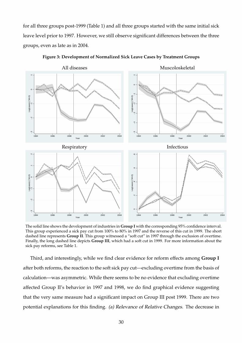
for all three groups post-1999 (Table 1) and all three groups started with the same initial sick

leave level prior to 1997. However, we still observe significant differences between the three

groups, even as late as in 2004.

Figure 3: Development of Normalized Sick Leave Cases by Treatment Groups

All diseases Muscoloskeletal

-.3

-.2

-.1

0.1

Log(

case

s) (

´94=

0)

1994 1996 1998 2000 2002 2004Year

-.5

-.4

-.3

-.2

-.1

0.1

Log(

case

s) (

´94=

0)

1994 1996 1998 2000 2002 2004Year

Respiratory Infectious

-.3

-.2

-.1

0.1

.2Lo

g(ca

ses)

(´9

4=0)

1994 1996 1998 2000 2002 2004Year

0.2

.4.6

.8Lo

g(ca

ses)

(´9

4=0)

1994 1996 1998 2000 2002 2004Year

The solid line shows the development of industries in Group I with the corresponding 95% confidence interval.This group experienced a sick pay cut from 100% to 80% in 1997 and the reverse of this cut in 1999. The shortdashed line represents Group II. This group witnessed a “soft cut” in 1997 through the exclusion of overtime.Finally, the long dashed line depicts Group III, which had a soft cut in 1999. For more information about thesick pay reforms, see Table 1.

Third, and interestingly, while we find clear evidence for reform effects among Group I

after both reforms, the reaction to the soft sick pay cut—excluding overtime from the basis of

calculation—was asymmetric. While there seems to be no evidence that excluding overtime

affected Group II’s behavior in 1997 and 1998, we do find graphical evidence suggesting

that the very same measure had a significant impact on Group III post 1999. There are two

potential explanations for this finding. (a) Relevance of Relative Changes. The decrease in

30

sick pay at the end of 1996 was heatedly debated in German society and led to strikes. The

main (media) focus was clearly on the decrease in the overall sick pay level. It is plausi-

ble that Group II did not react since the main reference point mattered here, which was the

decrease in the default federal level. About 50% of all employees experienced a decrease

in the level to 80% (Ridinger, 1997; Jahn, 1998). Hence the exclusion of overtime pay was,

relatively seen, negligible for affected workers. It may not even have been noticed by the

affected employees. After unions managed to negotiate the general sick pay level to remain

at 100%, they marketed and emphasized this success accordingly—but either did not men-

tion, or heavily down played the overtime cut. In 1999, by contrast, the exclusion of paid

overtime was the only regulatory change that made employees worse off. (b) LATE. Since

the model identifies the Local Average Treatment Effect (LATE), it could simply be that paid

overtime was more relevant for Group III than for Group II.

Finally, relating these findings to our model in Section 2, one can summarize that (i)

there is clear evidence for a significant and persistent decrease in the absence rate, βτ > 0

(Proposition 4a). Moreover, (ii) we find that the total percentage adjustment of contagious

diseases is smaller than the adjustment of non-contagious diseases and thus Proposition

4c, βnτ > βcτ, holds up. In addition, we find a large decrease in shirking βnτ > 0 while

the increase in presenteeism outweighs additional infections βcτ > 0 (Proposition 4b ). Fi-

nally, since (iii) βnτ − βcτ > 0, the reform being studied also led to an increase in infections

(Proposition 4b ).

5.2 Evidence from Regression Models: Sickness Adjustments by Dis-

eases

Disease-Specific Labor Supply Adjustments: Decomposing Moral Hazard

Estimating βτ, βnτ, and βcτ. Table 2 shows the results of the regression model in equation

(15) using different outcome variables: the logarithm of sick cases per 100 enrollees by the

disease categories total, musculoskeletal, digestive, infectious, respiratory, and injuries &

poisoning. Each column is one model as in equation (15). For illustrative purposes, we

31

solely show the coefficients of β1 to β4 and suppress the remaining ones. In the row below

the β1 to β4 coefficient estimates, we (a) display the results of an F-test β2− β1 = 0 to test the

effect of the sick pay level increase in 1999 for Group I relative to Group III. As discussed in

Section 4.3, the empirical models closely identify the theoretical model. For example, β1 in

the first row of the first column of Table 2 estimates βτ in equation (14) and tests Proposition

4a. The finding is then cross-checked by β2 − β1 = 0 which likewise test Proposition 4a

using the increase in sick pay as as an exogenous source of variation.

Note that the overtime exclusion, or “soft sick pay cut” as we call it, essentially also tests

Proposition 4a and the size and sign of βτ in equation (14) since any variant of making the

sick pay less generous could be interpreted as a decrease in sick pay. However, we believe

that the best suited coefficient estimates to test Propositions 4a-c are the ones resulting from

GroupIi ×′ 97−′ 98—the β1s for the different disease categories. These are the effects of the

initial reduction in the sick pay replacement rate from 100% to 80% in 1997/1998. However,

we double and cross-check the consistency and plausibility of these main β1 findings using

the effects of (i) the increase in the replacement rate from 80% to 100% in 1999 (β2 − β1), the

(ii) exclusion of overtime for Group II in 1997 (β3) and Group III and 1999 (β3 − β4), as well

as (iii) the overall development of the sick leave rates from 1999 to 2004—when the system

as a whole was more restrictive—relative to 1994 to 1996 (β2; β4).

One can summarize the following from Table 2: First, during the time when sick pay was

cut to 80%, in 1997 and 1998, we find overall decreases in the sickness rate by about 22% (β1

in column (1)). This reflects βτ in equation (14), i.e., the total moral hazard effect. As seen,

β1 is highly significant and clearly larger than zero, which confirms Proposition 4a. Related

to the decrease in sick pay of 20%, one obtains a sickness rate elasticity with respect to the

replacement rate of about 1. Decreases of similar size are found for respiratory and digestive

diseases (columns (3) and (4)).

32

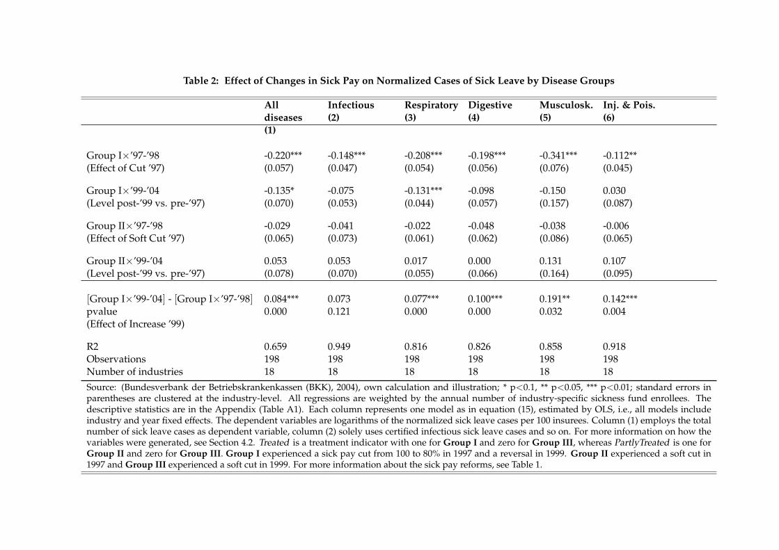
Table 2: Effect of Changes in Sick Pay on Normalized Cases of Sick Leave by Disease Groups

Alldiseases(1)

Infectious(2)

Respiratory(3)

Digestive(4)

Musculosk.(5)

Inj. & Pois.(6)

Group I×’97-’98 -0.220*** -0.148*** -0.208*** -0.198*** -0.341*** -0.112**(Effect of Cut ’97) (0.057) (0.047) (0.054) (0.056) (0.076) (0.045)

Group I×’99-’04 -0.135* -0.075 -0.131*** -0.098 -0.150 0.030(Level post-’99 vs. pre-’97) (0.070) (0.053) (0.044) (0.057) (0.157) (0.087)

Group II×’97-’98 -0.029 -0.041 -0.022 -0.048 -0.038 -0.006(Effect of Soft Cut ’97) (0.065) (0.073) (0.061) (0.062) (0.086) (0.065)

Group II×’99-’04 0.053 0.053 0.017 0.000 0.131 0.107(Level post-’99 vs. pre-’97) (0.078) (0.070) (0.055) (0.066) (0.164) (0.095)

[Group I×’99-’04] - [Group I×’97-’98] 0.084*** 0.073 0.077*** 0.100*** 0.191** 0.142***pvalue 0.000 0.121 0.000 0.000 0.032 0.004(Effect of Increase ’99)

R2 0.659 0.949 0.816 0.826 0.858 0.918Observations 198 198 198 198 198 198Number of industries 18 18 18 18 18 18Source: (Bundesverbank der Betriebskrankenkassen (BKK), 2004), own calculation and illustration; * p<0.1, ** p<0.05, *** p<0.01; standard errors inparentheses are clustered at the industry-level. All regressions are weighted by the annual number of industry-specific sickness fund enrollees. Thedescriptive statistics are in the Appendix (Table A1). Each column represents one model as in equation (15), estimated by OLS, i.e., all models includeindustry and year fixed effects. The dependent variables are logarithms of the normalized sick leave cases per 100 insurees. Column (1) employs the totalnumber of sick leave cases as dependent variable, column (2) solely uses certified infectious sick leave cases and so on. For more information on how thevariables were generated, see Section 4.2. Treated is a treatment indicator with one for Group I and zero for Group III, whereas PartlyTreated is one forGroup II and zero for Group III. Group I experienced a sick pay cut from 100 to 80% in 1997 and a reversal in 1999. Group II experienced a soft cut in1997 and Group III experienced a soft cut in 1999. For more information about the sick pay reforms, see Table 1.

Second, musculoskeletal diseases is the category that represents best the non-contagious

disease category n in our model in Section 2. As a result of the sick pay cut, the sick leave

rate of musculoskeletal diseases decreased overproportionally by 34% (column (5), β1). The

overproportional decrease for musculoskeletal diseases, which is composed of 70% back

pain cases, fits the common perception that the labor supply of this category is particularly

elastic and prone to shirking behavior. Equation (9) of our model illustrates the analyti-

cal derivation of βnτ. βnτ, which is represented by β1 in column (5) of Table 2, equals the

decrease in shirking as sick pay decreases.

Third, infectious diseases, ICD-10 codes A00-B99, is the category that best represents

best the contagious disease category c in our model. This estimate represents the βcτ in our

model in equation (11). As β1 in column (2) of Table 2 shows, the infectious disease rate fell

under proportionally by an estimated 15% as a response to the sick pay cut in 1997/1998.

Note that this estimate is likely to be upward biased, since the pre-1997 common time trend

for infectious diseases is not 100% clean as Figure 3d nicely illustrates: While there is strong

convincing support for an overall common time trend among all three groups and over the

11 year time period from 1994 to 2004, the only outlier is the pre-reform years 1994/1995,

where we observe an above-trend increase among Group I. Considering this and assessing

the overall infectious disease trend picture in Figure 3d, the estimated decrease of 15% ap-

pears upwardly biased and the true estimate seems to tend more towards zero. In any case,

while the findings suggest that βnτ > βcτ as formulated in Hypothesis 1 and Proposition

4c, it is also clear that βτ > 0 holds, meaning that the reform led to a decrease in overall

sickness absence.

Testing the Robustness of the Identified Effects. Table 2 also provides a series of ad-

ditional estimates that allow us to check the plausibility and consistency of the identified

model parameters βτ, βnτ, and βcτ.

First of all, the reaction of sick leave due to injuries & poisoning in column (6) of Ta-

ble 2 serves as a robustness test since 50% of all injuries & poisoning absences are due to

workplace accidents (Bundesverbank der Betriebskrankenkassen (BKK), 2004). The first bill

that cut sick pay, however, excluded sick leave due to workplace accidents from the cuts

34

(see Section 3.2). Indeed, as see by β1 in column (6), the injuries & poisoning absence rate

decreased underproportionally by almost exactly half the rate than the overall rate, namely

by 11.2% instead of 22%.

Second, the β2 estimate provides the change in sickness rates in the post-1999 era rela-

tive to the pre-1997 era for Group I. Meanwhile, the F-test, β2-β1 = 0, yields the effect of

an increase in the replacement rate to 100% in 1999. Thus β2 reflects the long-term impact

after a series of reforms that made the overall system more restrictive and shows a decrease

of 13.5% at the 10 percent significance level for all diseases. The same is true for respiratory

diseases, while the coefficients are relatively large but not statistically significant for infec-

tious (-7.5%), digestive (-9.8%), and musculoskeletal (-15.0%) diseases.30 β2-β1 is highly

significant for all disease categories but infectious diseases. Column (1) suggests that the

overall rate increased again by 8.4% after the reversal. Column (5) also confirms our find-

ings above and strongly suggests that musculoskeletal diseases, i.e. the group respresenting

non-contagious diseases in the model, reacted overproportionally with an increase of 19.1%

as a reaction to the increase in sick pay to 100%.

Third, all separate β3 and β4 estimates are imprecise and relatively small in size mean-

ing that—in an regression framework that employs industry and year fixed effects—we are

unable to detect significant sick leave rate changes in response to the mild sick leave cuts

that excluded overtime from the basis of calculation. However, this is at least partly a func-

tion of the statistical power that our data offer. Note that all coefficients carry the expected

sign and most magnitudes lie around 3 to 5%.31 In addition, when formally carrying out an

F-test of β3 − β4 = 0 to test the effect of the overtime exclusion in 1999 for Group III, we ob-

tain enough precision and significant decreases in the sick leave rates. Also note that, while

power can be an issue when it comes to the identification of small changes, as the R-squared

in Table 2 indicates, our models are able to explain between 66% and 95% of the variation in

sick leave rates over time and between industries.30Remember that we likely overestimate the behavioral reactions for infections due to a deviation from the

common time trend pre-1997, as discussed above and shown in Figure 3d.31Recall again that the 1999 exclusion of overtime was effective for Group III but not for Group II while the

opposite was true when the first reform was implemented. This means that the positive signs of β4 actuallyrepresent decreases in the sick leave rate as a result of the overtime exclusion.

35

In conclusion, all findings strongly confirm the robustness of our results for βτ, βnτ, and

βcτ above. Moreover, they are entirely in line with the graphical evidence (see Figure 3) as

well as our discussion above: overall sickness rates in the Group I clearly increased again

after the sick pay cut was reversed. However, the increase kicked-in with a lag of about

one year and we observe time persistence in the behavioral reactions—the reform-induced

sick pay gaps among the three groups did not entirely close until the end of the observation

period. Finally, the labor supply elasticities are smallest for infectious diseases and largest

for musculoskeletal diseases. The former category represents non-contagious and the latter

non-contagious diseases.

Does the Decrease in Shirking Outweigh the Negative Externalities of Contagious Pre-

senteeism?

Estimating βnτ-βcτ. Next, we pool the different disease-industry-year observations and run

regression models as in equation (16). Following Proposition 4c, this allows us to directly

carry out the following statistical tests βnτ = βcτ.

Column (1) of Table 3 simply replicates column (5) of Table 2 and carries 198 observa-

tions. Column (5) of Table 2 estimated the impact on musculoskeletal diseases, our main

reference group for non-contagious diseases.

Column (2) adds our main contagious disease category infectious diseases and has 396

observations. With musculoskeletal diseases as the baseline category, the four triple DiD in-

teraction terms (i) GroupIi×′ 97−′ 98× In f ectious, (ii) GroupIi×′ 99−′ 04× In f ectious, (iii)

GroupI Ii×′ 97−′ 98× In f ectious, and (iv) GroupI Ii×′ 99−′ 04× In f ectious —or γi1− γi5—

directly test Hypothesis 1 (βnτ = βcτ). What has already been suggested in Table 2 above,

can now be demonstrated with statistical certainty in column (2) of Table 3: βcτ-βnτ=19.3

percentage points, meaning that the sick pay cut induced decrease in the contagious sick

leave rate was a significant 19.3 percentage points smaller than the decrease in the non-

contagious sick leave rate (14.8% vs. 34.1%, see columns (2) and (5) of Table 2). Again, this

is likely an underestimate since we likely overestimate βcτ.

36

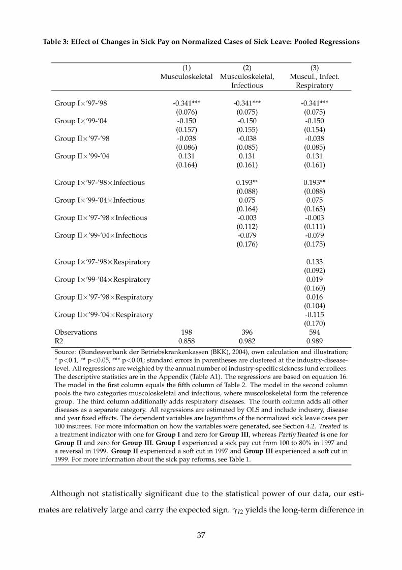
Table 3: Effect of Changes in Sick Pay on Normalized Cases of Sick Leave: Pooled Regressions

(1) (2) (3)Musculoskeletal Musculoskeletal, Muscul., Infect.

Infectious Respiratory

Group I×’97-’98 -0.341*** -0.341*** -0.341***(0.076) (0.075) (0.075)

Group I×’99-’04 -0.150 -0.150 -0.150(0.157) (0.155) (0.154)

Group II×’97-’98 -0.038 -0.038 -0.038(0.086) (0.085) (0.085)

Group II×’99-’04 0.131 0.131 0.131(0.164) (0.161) (0.161)

Group I×’97-’98×Infectious 0.193** 0.193**(0.088) (0.088)

Group I×’99-’04×Infectious 0.075 0.075(0.164) (0.163)

Group II×’97-’98×Infectious -0.003 -0.003(0.112) (0.111)

Group II×’99-’04×Infectious -0.079 -0.079(0.176) (0.175)

Group I×’97-’98×Respiratory 0.133(0.092)

Group I×’99-’04×Respiratory 0.019(0.160)

Group II×’97-’98×Respiratory 0.016(0.104)

Group II×’99-’04×Respiratory -0.115(0.170)

Observations 198 396 594R2 0.858 0.982 0.989Source: (Bundesverbank der Betriebskrankenkassen (BKK), 2004), own calculation and illustration;* p<0.1, ** p<0.05, *** p<0.01; standard errors in parentheses are clustered at the industry-disease-level. All regressions are weighted by the annual number of industry-specific sickness fund enrollees.The descriptive statistics are in the Appendix (Table A1). The regressions are based on equation 16.The model in the first column equals the fifth column of Table 2. The model in the second columnpools the two categories muscoloskeletal and infectious, where muscoloskeletal form the referencegroup. The third column additionally adds respiratory diseases. The fourth column adds all otherdiseases as a separate category. All regressions are estimated by OLS and include industry, diseaseand year fixed effects. The dependent variables are logarithms of the normalized sick leave cases per100 insurees. For more information on how the variables were generated, see Section 4.2. Treated isa treatment indicator with one for Group I and zero for Group III, whereas PartlyTreated is one forGroup II and zero for Group III. Group I experienced a sick pay cut from 100 to 80% in 1997 anda reversal in 1999. Group II experienced a soft cut in 1997 and Group III experienced a soft cut in1999. For more information about the sick pay reforms, see Table 1.

Although not statistically significant due to the statistical power of our data, our esti-

mates are relatively large and carry the expected sign. γI2 yields the long-term difference in

37

the adjustment rate for musculoskeletal vs. infectious diseases illustrating again that infec-

tious sick leave rates are much less responsive, also in the long-run. The triple DiD estimate

γI4 shows the long-term effect post-1999 vs. pre-1997 for Group II as compared to Group

III and musculoskeletal vs. infectious diseases. The visual equivalent to γI2 and γI4 is to

compare the post-1999 sickness rate gaps for musculoskeletal vs. infectious diseases rela-

tive to the pre-1997 gaps in Figures 3b vs. 3d. Figures 3b and 3d illustrate very nicely and

even more clearly than Table 3 that there was basically no behavioral reaction for infectious

diseases while one observes substantial behavioral reactions for musculoskeletal diseases.

Finally, column (3) serves as yet another robustness check and additionally adds respira-

tory diseases to the data set. While not all respiratory diseases are contagious, this category

contains “influenza (J09)”, commonly referred to as the flu. As above, the four triple inter-

action terms identify the differential effect relative to the baseline category musculoskeletal

diseases. Again, although we lack statistical power, there is suggestive evidence that the res-

piratory sick leave rate decreased by about 13% less than the non-contagious baseline (γR1).

Similarly, the impact of the soft cut for Group III seems to have been less strong (γR3-γR4).

6 Conclusion

Empirically identifying presenteeism behavior is extremely challenging, yet crucial in order

to test for one major economic justification for publicly provided sick pay: that being the

negative externalities associated with contagious presenteeism. Contagious presenteeism

refers to the phenomenon when employees with infectious diseases go to work sick and

infect co-workers and customers. Such behavior is a major public health issue and one

driving force of the spread of contagious diseases. If contagion is unobservable, which is

unusually the case at the beginning of a sickness episode, then state regulation may reduce

market inefficiencies by providing monetary incentives to stay home when sick. If such

monetary incentives work, and economic theory as well empirical studies strongly suggest

that they do, then public sick pay schemes reduce contagious presenteeism and the spread

of diseases.

38

To our knowledge, this study is the first that theoretically derives and empirically im-

plements tests for the existence of contagious presenteeism and negative externalities in

sickness insurance schemes. First, our model theoretically defines different possible cases

of workplace absence behavior under contagious and non-contagious continuous sickness

levels. As such, we also decompose classical moral hazard into (i) shirking behavior, and

(ii) contagious presenteeism. Case (i) does not imply negative health spillovers, whereas

case (ii) does. We derive conditions to be able to test for moral hazard and its decomposed

elements (i) and (ii). Then, we exploit two German sick pay reforms and administrative

physician-certified sick leave data at the industry-level to provide empirical evidence for

the existence of contagious presenteeism, which we indeed find. However, we also show

that, in Germany, with one of the most generous sick leave systems worldwide, the reduc-

tion in shirking behavior was larger than the increase in the infectious disease rate due to

contagious presenteeism when sick pay was cut from a baseline level of 100%.

Our proposed method can be applied to different settings in order to test for the existence

and the degree of contagious presenteeism, shirking behavior, and the overall level of moral

hazard. Important fields of applications include (a) contagious presenteeism by teachers or

school kids, e.g., induced by the (non-)generosity of teacher or parental sick pay schemes

that may or may not cover sickness of children. Another relevant application would be to

test for (b) contagious presenteeism behavior by service sector employees with a high degree

of customer contact, e.g., induced by the (non-)generosity of a firm-level sick pay scheme.

As a last example, (c) contagious presenteeism behavior by health care workers can be life-

threatening for patients, but potentially be minimized by optimized sick pay schemes. Note

that our test can be carried out using many different types of data, including school-level,

firm-level data, or hospital-level data.

More research is needed in order to better understand how exactly contagious presen-

teeism leads to infections of co-workers and customers and affect overall workplace produc-

tivity. Firm-level and employee-level compensation strategies to dampen sickness-related

productivity losses are also fruitful related research questions.

39

References

Arnott, R. and J. Stiglitz (1991). The welfare economics of moral hazard. In H. Louberg (Ed.),Risk, Information and Insurance, pp. 91–121. Springer Netherlands.

Aronsson, G., K. Gustafsson, and M. Dallner (2000). Sick but yet at work. An empirical studyof sickness presenteeism. Journal of Epidemiology & Community Health 54(7), 502–509.

Askildsen, J. E., E. Bratberg, and Ø. A. Nilsen (2005). Unemployment, labor force composi-tion and sickness absence: A panel study. Health Economics 14(11), 1087–1101.

Barmby, T. and M. Larguem (2009). Coughs and sneezes spread diseases: An empiricalstudy of absenteeism and infectious illness. Journal of Health Economics 28(5), 1012–1017.

Barmby, T., J. Sessions, and J. G. Treble (1994). Absenteeism, efficiency wages and shirking.Scandinavian Journal of Economics 96(4), 561–566.

Bhattacharya, J. and M. Packalen (2012). The other ex ante moral hazard in health. Journal ofHealth Economics 31(1), 135–146.

Blank, P. R., M. M. Schwenkglenks, and T. D. Szucs (2009). Vaccination coverage rates ineleven European countries during two consecutive influenza seasons. Journal of Infec-tion 58(6), 446–458.

Blien, U., E. J. Jahn, G. Stephan, M. Knig, and J. Mller (2009). Impacts of minimum wages:a microdata analysis for the german construction sector. International Journal of Man-power 30(7), 716–741.

Boots, S. W., K. Martinson, and A. Danziger (2009). Employers’ perspectives on San Fran-cisco’s paid sick leave policy. Technical report, The Urban Institute. http://www.urban.org/publications/411868.html, last accessed on April 5, 2012.

Brown, S. (1994). Dynamic implications of absence behaviour. Applied Economics 26, 1163–1175.

Brown, S. and J. G. Sessions (1996). The economics of absence: Theory and evidence. Journalof Economic Surveys 10(1), 23–53.

Brown, S. and J. G. Sessions (2004). Absenteeism, presenteeism, and shirking. EconomicIssues 9(1), 15–23.

Bruine de Bruin, W., A. Parker, and J. Maurer (2011). Assessing small non-zero perceptionsof chance: The case of H1N1 (swine) flu risks. Journal of Risk and Uncertainty 42(2), 145–159.

Bundesverbank der Betriebskrankenkassen (BKK) (1994-2004). Krankheitsartenstatistik. BKKBundesverband.

Busse, R. and A. Riesberg (2004). Health care systems in transition: Germany (1 ed.). WHORegional Office for Europe on behalf of the European Observatory on Health Systems andPolicies.

40

Centers for Disease Control and Prevention (2014a). Final state-level influenza vaccinationcoverage estimates for the 2010-11 season – United States, National Immunization Survey andBehavioral Risk Factor Surveillance System, August 2010 through May 2011. CDC. http://www.cdc.gov/flu/fluvaxview/coverage_1011estimates.htm, last accessedon June 19, 2014.

Centers for Disease Control and Prevention (2014b). Seasonal Influenza (Flu). CDC. http://www.cdc.gov/flu/about/disease/index.htm, last accessed on September 9, 2014.

Chatterji, M. and C. J. Tilley (2002). Sickness, absenteeism, presenteeism, and sick pay. Ox-ford Economic Papers 54, 669–687.

Dale-Olsen, H. (2013). Absenteeism, efficiency wages, and marginal taxes. ScandinavianJournal of Economics 115(4), 1158–1185.

Dale-Olsen, H. (2014). Sickness absence, sick leave pay, and pay schemes. Labour 28(1),40–63.

De Paola, M., V. Scoppa, and V. Pupo (2014). Absenteeism in the Italian public sector: Theeffects of changes in sick leave policy. Journal of Labor Economics 32(2), 337–360.

Earn, D. J. D., P. W. Andrews, and B. M. Bolker (2014). Population-level effects of suppressingfever. Proceedings of the Royal Society B: Biological Sciences 281(1778).

Eibich, P., H. Schmitz, and N. R. Ziebarth (2012). Add-on premiums increase price trans-parency: More policy holders switch health plans. DIW Economic Bulletin 2(2), 15–24.

Einav, L., A. Finkelstein, S. P. Ryan, P. Schrimpf, and M. R. Cullen (2013). Selection on moralhazard in health insurance. The American Economic Review 103(1), 178–219.

Felder, S. (2008). To wait or to pay for medical treatment? restraining ex-post moral hazardin health insurance. Journal of Health Economics 27(6), 1418–1422.

Fevang, E., S. Markussen, and K. Røed (2014). The sick pay trap. Journal of Labor Eco-nomics 32(2), 305–336.

German Federal Statistical Office (1998). Statistical Yearbook 1998 for the Federal Republic ofGermany. Metzler-Poeschel.

German Federal Statistical Office (2014). Federal Health Monitoring. www.gbe-bund.de, lastaccessed on October 25, 2014.

Gruber, J. (1994). The incidence of mandated maternity benefits. American Economic Re-view 84(3), 622–641.

Hans Bockler Stiftung (2014). WSI Tarifarchiv. Deutscher Gewerkschaftsbund (DGB). http://www.boeckler.de/index_wsi_tarifarchiv.htm, last accessed on June 19, 2014.

Heymann, J., H. J. Rho, J. Schmitt, and A. Earle (2009). Contagion nation: a comparisonof paid sick day policies in 22 countries. Technical Report 2009-19, Center for Economicand Policy Research (CEPR). http://www.cepr.net/documents/publications/paid-sick-days-2009-05.pdf, last accessed on April 5, 2012.

41

Ichino, A. and G. Maggi (2000). Work environment and individual background: Explain-ing regional shirking differentials in a large Italian firm. The Quarterly Journal of Eco-nomics 115(3), 1057–1090.

Ichino, A. and E. Moretti (2009). Biological gender differences, absenteeism, and the earningsgap. American Economic Journal: Applied Economics 1(1), 183–218.

Ichino, A. and R. T. Riphahn (2005). The effect of employment protection on worker effort.A comparison of absenteeism during and after probation. Journal of the European EconomicAssociation 3(1), 120–143.

Jahn, J. (1998). Lohnfortzahlung: Gerichte stehen vor Herkulesaufgabe. Handelsblatt July, 2,4.

Johansson, P. and M. Palme (1996). Do economic incentives affect work absence? Empiricalevidence using Swedish micro data. Journal of Public Economics 59(1), 195–218.

Johansson, P. and M. Palme (2002). Assessing the effect of public policy on worker absen-teeism. Journal of Human Resources 37(2), 381–409.

Johansson, P. and M. Palme (2005). Moral hazard and sickness insurance. Journal of PublicEconomics 89(9-10), 1879–1890.

Karlsson, M., T. Nilsson, and S. Pichler (2014). The impact of the 1918 Spanish flu epidemicon economic performance in Sweden. Journal of Health Economics 36(0), 1–19.

Kermack, W. and A. McKendrick (1927). A contribution to the mathematical theory of epi-demics. Proceedings of the Royal Society of London. Series A 115(772), 700–721.

Lovell, V. (2003). No time to be sick: Why everyone suffers when workers don’t have paidsick leave. Policy report, Institute for Womens Policy Research. http://www.iwpr.org/publications/pubs/, last accessed at March 19, 2014.

Markussen, S. (2012). The individual cost of sick leave. Journal of Population Economics 25(4),1287–1306.

Markussen, S., A. Mykletun, and K. Røed (2012). The case for presenteeism: Evidence fromNorway’s sickness insurance program. Journal of Public Economics 96(11), 959–972.

Markussen, S., K. Røed, O. J. Røgeberg, and S. Gaure (2011). The anatomy of absenteeism.Journal of Health Economics 30(2), 277–292.

Maurer, J. (2009). Who has a clue to preventing the flu? Unravelling supply and demandeffects on the take-up of influenza vaccinations. Journal of Health Economics 28(3), 704–717.

Medizinischer Dienst der Krankenversicherung (MDK) (2014). www.mdk.de, last accessedat April 27, 2014.

Mullahy, J. (1999). It’ll only hurt a second? Microeconomic determinants of who gets flushots. Health Economics 8(1), 9–24.

Newhouse, J. P. (2006). Reconsidering the moral hazard-risk avoidance tradeoff. Journal ofHealth Economics 25(5), 1005–1014.

42

Nordberg, M. and K. Røed (2009). Economic incentives, business cycles, and long-termsickness absence. Industrial Relations 48(2), 203–230.

Nyman, J. A. (1999). The economics of moral hazard revisited. Journal of Health Eco-nomics 18(6), 811–824.

Pauly, M. (1983). More on moral hazard. Journal of Health Economics 2(1), 81–85.

Pauly, M. V. (1974). Overinsurance and public provision of insurance: The roles of moralhazard and adverse selection. The Quarterly Journal of Economics 88(1), 44–62.

Pauly, M. V., S. Nicholson, D. Polsky, M. L. Berger, and C. Sharda (2008). Valuing reductionsin on-the-job illness: ’presenteeism’ from managerial and economic perspectives. HealthEconomics 17(4), 469–485.

Philipson, T. (2000). Economic epidemiology and infectious diseases. In A. J. Culyer and J. P.Newhouse (Eds.), Handbook of Health Economics, Volume 1 of Handbook of Health Economics,Chapter 33, pp. 1761–1799. Elsevier.

Pichler, S. (2014). Sickness absence, moral hazard, and the business cycle. Health Economics.forthcoming.

Puhani, P. A. and K. Sonderhof (2010). The effects of a sick pay reform on absence and onhealth-related outcomes. The Journal of Health Economics 29(2), 285–302.

Rattenhuber, P. (2011). Building the minimum wage: Germany’s first sectoral minimumwage and its impact on wages in the construction industry. Discussion papers, GermanInstitute for Economic Research (DIW Berlin) 1111.

Ridinger, R. (1997). Einfluss arbeitsrechtlicher Regelungen auf dieBeschaftigungsentwicklung im Handwerk–Ergebnisse von Befragungen von Handw-erksbetrieben im 3. Quartal 1997. Technical report, Zentralverband des DeutschenHandwerks. http://www.zdh.de, last accessed on June 19, 2009.

Riphahn, R. T. (2004). Employment protection and effort among German employees. Eco-nomics Letters 85, 353–357.

Ross, R. (1916). An application of the theory of probabilities to the study of a priori pathom-etry. Part I. Proceedings of the Royal Society of London. Series A 92(638), 204–230.

Rossin-Slater, M., C. J. Ruhm, and J. Waldfogel (2013). The effects of California’s Paid FamilyLeave Program on mothers leave? taking and subsequent labor market outcomes. Journalof Policy Analysis and Management 32(2), 224–245.

Ruhm, C. J. (1998). The economic consequences of parental leave mandates: Lessons fromEurope. The Quarterly Journal of Economics 113(1), 285–317.

Sandy, R. and R. F. Elliott (2005). Long-term illness and wages: The impact of the risk ofoccupationally related long-term illness on earnings. Journal of Human Resources 40(3),744–768.

Schmitz, H. and N. R. Ziebarth (2013). How framing prices affects the consumer price sensi-tivity of health plan choice. mimeo, Cornell University. http://www.human.cornell.edu/pam/people/nicolas_ziebarth.cfm, last accessed on December 15, 2013.

43

Scoppa, V. and D. Vuri (2014). Absenteeism, unemployment and employment protectionlegislation: evidence from Italy. IZA Journal of Labor Economics 3(1), 1–25.

SOEPGroup (2008). German Socio-economic Panel Study (SOEP), data of the years 1984 2007.DOI: 10.5684/soep.v24.

Thomas, M. (2015). The impact of mandated maternity benefits on the gender differential inpromotions: Examining the role of adverse selection. Technical report. mimeo.

Uscher-Pines, L., J. Maurer, and K. M. Harris (2011). Racial and ethnic disparities in uptakeand location of vaccination for 2009-H1N1 and seasonal influenza. American Journal ofPublic Health 101(7), 1252–1255.

Waldfogel, J. (1998). Understanding the “family gap” in pay for women with children. Jour-nal of Economic Perspectives 12(1), 137–156.

World Health Organization (2014). Influenza (Seasonal). WHO. http://www.who.int/mediacentre/factsheets/fs211/en/, last accessed on June 19, 2014.

Ziebarth, N. R. (2013). Long-term absenteeism and moral hazard—Evidence from a naturalexperiment. Labour Economics 24, 277292.

Ziebarth, N. R. and M. Karlsson (2010). A natural experiment on sick pay cuts, sicknessabsence, and labor costs. Journal of Public Economics 94(11-12), 1108–1122.

Ziebarth, N. R. and M. Karlsson (2014). The effects of expanding the generosity of the statu-tory sickness insurance system. Journal of Applied Econometrics 29(2), 208–230.

44

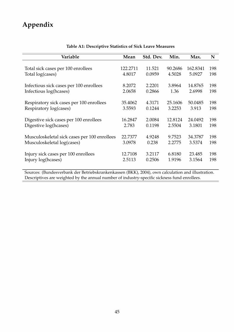
Appendix

Table A1: Descriptive Statistics of Sick Leave Measures

Variable Mean Std. Dev. Min. Max. N

Total sick cases per 100 enrollees 122.2711 11.521 90.2686 162.8341 198Total log(cases) 4.8017 0.0959 4.5028 5.0927 198

Infectious sick cases per 100 enrollees 8.2072 2.2201 3.8964 14.8765 198Infectious log(hcases) 2.0658 0.2866 1.36 2.6998 198

Respiratory sick cases per 100 enrollees 35.4062 4.3171 25.1606 50.0485 198Respiratory log(cases) 3.5593 0.1244 3.2253 3.913 198

Digestive sick cases per 100 enrollees 16.2847 2.0084 12.8124 24.0492 198Digestive log(hcases) 2.783 0.1198 2.5504 3.1801 198

Musculoskeletal sick cases per 100 enrollees 22.7377 4.9248 9.7523 34.3787 198Musculoskeletal log(cases) 3.0978 0.238 2.2775 3.5374 198

Injury sick cases per 100 enrollees 12.7108 3.2117 6.8180 23.485 198Injury log(hcases) 2.5113 0.2506 1.9196 3.1564 198

Sources: (Bundesverbank der Betriebskrankenkassen (BKK), 2004), own calculation and illustration.Descriptives are weighted by the annual number of industry-specific sickness fund enrollees.

45

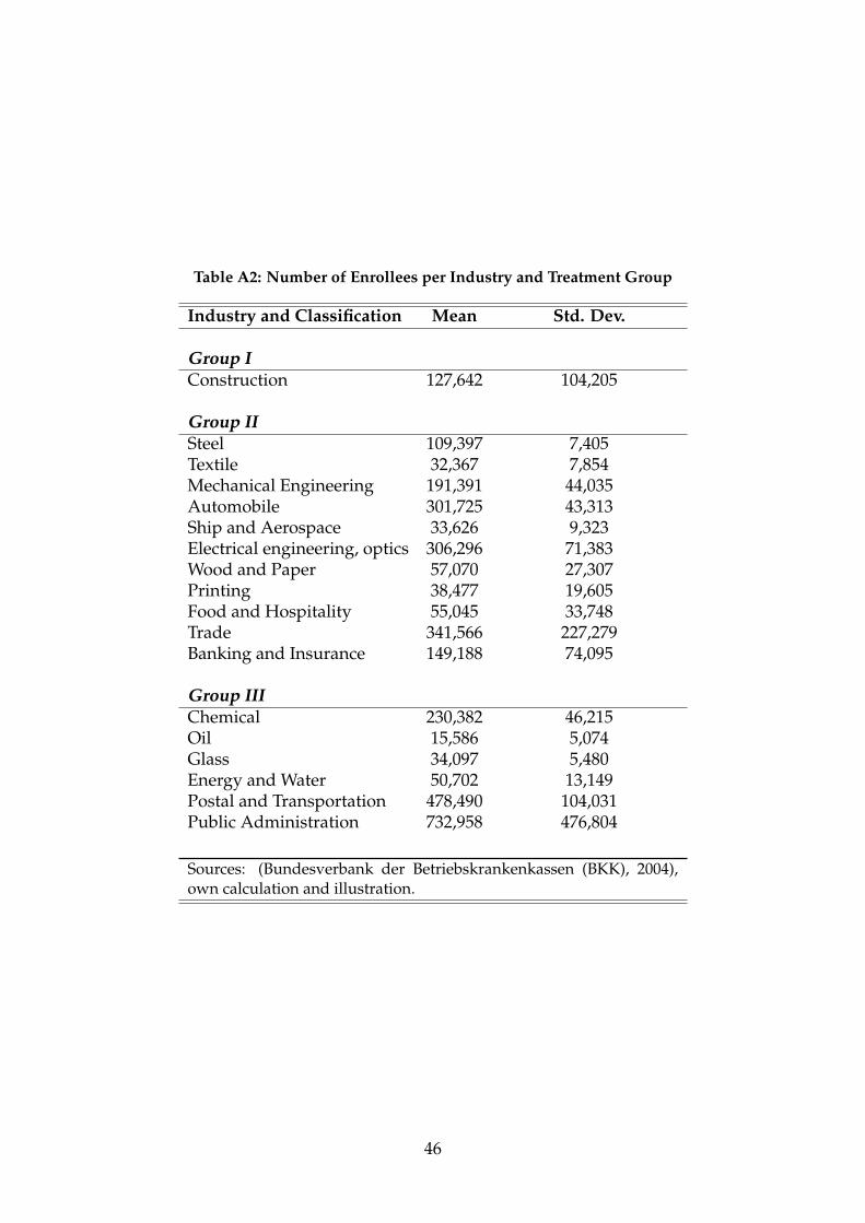
Table A2: Number of Enrollees per Industry and Treatment Group

Industry and Classification Mean Std. Dev.

Group IConstruction 127,642 104,205

Group IISteel 109,397 7,405Textile 32,367 7,854Mechanical Engineering 191,391 44,035Automobile 301,725 43,313Ship and Aerospace 33,626 9,323Electrical engineering, optics 306,296 71,383Wood and Paper 57,070 27,307Printing 38,477 19,605Food and Hospitality 55,045 33,748Trade 341,566 227,279Banking and Insurance 149,188 74,095

Group IIIChemical 230,382 46,215Oil 15,586 5,074Glass 34,097 5,480Energy and Water 50,702 13,149Postal and Transportation 478,490 104,031Public Administration 732,958 476,804

Sources: (Bundesverbank der Betriebskrankenkassen (BKK), 2004),own calculation and illustration.

46