1

The Quality of China’s GDP Statistics

Since the 1998 “wind of falsification and embellishment,” Chinese official GDP statistics have repeatedly come under scrutiny. This paper evaluates the quality of China’s GDP statistics in four stages. First, it reviews past and ongoing suspicions of the quality of GDP data and examines the evidence. Second, it documents the institutional framework for data compilation and concludes on the implications for data quality. Third, it asks how the National Bureau of Statistics could possibly go about credibly falsifying GDP data without being found out. Fourth, it examines if the first-and second-digit distributions of official GDP data conform to established data regularities (Benford’s Law). The findings are that the supposed evidence for GDP data falsification is not compelling, that the NBS has much institutional scope for falsifying GDP data, and that certain manipulations of nominal and real data would be virtually undetectable. Official GDP data, however, exhibit few statistical anomalies (conform to Benford’s Law) and the NBS thus either makes no significant use of its scope to falsify data, or is aware of statistical data regularities when it falsifies data. Journal of Economic Literature classification codes. all China:

C82 Data Collection and Data Estimation Methodology; Computer Programs — Methodology for Collecting, Estimating, and Organizing Macroeconomic Data

R1 General Regional Economics P27 Socialist Systems and Transitional Economies — Performance and Prospects O53 Economywide Country Studies — Asia including Middle East

Keywords (all: China): accuracy of national statistics; national income accounting; compilation of GDP and sectoral value-added, national statistical system; Benford’s Law.

Carsten A. Holz* Stanford Center for International Development, Stanford University

366 Galvez Street, Stanford, CA 94305-6015 Present address:

Social Science Division, Hong Kong University of Science & Technology (Clear Water Bay, Kowloon, Hong Kong)

E-mail: carstenholz@gmail.com, socholz@ust.hk +852 6351-5956

27 November 2013

* The author is professor of economics in the Social Science Division at the Hong Kong University of Science & Technology. The first version of this paper was written while on no-pay leave from HKUST to visit the Stanford Center for International Development at Stanford University. Financial support from the Stanford Center for International Development, under Nicholas Hope, is gratefully acknowledged. I am also grateful for comments and suggestions received from seminar participants at The Stanford Center for International Development (23 April 2013), the China Social Science Workshop at Stanford University (13 May 2013), and the East Asian Institute at National University of Singapore (10 October 2013), as well as from participants in the GEP China/ifo/CEPII Conference at the University of Nottingham Ningbo China (7 November 2013).

2

The Quality of China’s GDP Statistics

Carsten A. Holz

Contents

1. Introduction ................................................................................................................................4

2. Questions about Chinese Data Quality, and Technical Limitations ..........................................5 2.1 The 1998 Wind of Falsification and Embellishment ...........................................................5 2.2 Censuses and Benchmark Revisions ....................................................................................6 2.3 Annual Revisions .................................................................................................................8 2.4 Three Approaches to Calculating GDP ................................................................................9 2.5 Summed Provincial Vs. National Values.............................................................................9 2.6 Alternative Data Series ......................................................................................................10 2.7 Value-added of a Subset of Industry Exceeds Value-added of All of Industry .................10 2.8 Military Value-added .........................................................................................................12 2.9 Evaluation of Official GDP Compilation Methods ...........................................................13 2.10 Summary .....................................................................................................................14

3. Institutional Scope for Data Falsification ................................................................................14

4. How to Credibly Falsify China’s Official GDP Statistics .......................................................17 4.1 Scope for falsification of nominal GDP.............................................................................17 4.2 Scope for falsification of real GDP growth rates ...............................................................19

4.2.1 Sectoral real VA (and GDP) ..................................................................................20 4.2.2 Aggregate real expenditures ..................................................................................22

5. Benford’s Law .........................................................................................................................23 5.1 Introduction to Benford’s Law...........................................................................................23 5.2 Benford’s Law and Chinese National Income and Product Accounts Data ......................26

6. Conclusions ..............................................................................................................................27

3

Tables Table 1. Annual Rebisions to National Value-Added, Real GDP Growth Rates ................35 Table 2. Summed Provincial Value-Added Divided by GDP .............................................37 Table 3. Reliability of GDP Data Compilation Methods (2000) .........................................42 Table 4. Average Annual Real GDP Growth Rates .............................................................46 Table 5. Average Annual Real Growth Rates of Aggregate Expenditures ..........................47 Table 6. Significance Levels of Deviations of Actual Data from the Benford Distribution48 Figures Figure 1. Nominal GDP Divided by Aggregate Expenditures ..............................................36 Figure 2. Average Annual Growth Rates of Product Quantities Vs. Real Value-Added ......38 Figure 3. DRIE Share in Value-Added of Industry ...............................................................39 Figure 4. DRIE Share in Industry Employment ....................................................................40 Figure 5. DRIE Value-added, Value-added Tax Payable, GOV ...........................................41 Figure 6. Primary Sector Deflators........................................................................................44 Figure 7. Industry Deflators ..................................................................................................44 Figure 8. Tertiary Sector Deflators........................................................................................45 Figure 9. Alternative GDP Deflators .....................................................................................46 Figure 10. Nominal Data and Benford’s Law .........................................................................50 Figure 11. Deflators, Real Growth Rates and Benford’s Law ................................................51 Abbreviations b Billion CPI Consumer Price Index DRIE Directly reporting industrial enterprise GDP Gross domestic product GOV Gross output value m Million NBS National Bureau of Statistics NIPA National Income and Product Accounts PRC People’s Republic of China SOE State-owned enterprise VA Value-added VAT Value-added tax yuan Yuan Renminbi

4

1. Introduction

Chinese official statistics have a bad name. It doesn’t seem to matter which Chinese statistics one looks at. There is the discrepancy between the official Beijing air quality measurements and the air quality measurements conducted by the U.S. Embassy in Beijing atop its embassy building: one day in October 2011, the Chinese official reading was “slightly polluted” while the U.S. reading was “crazy bad” (later revised to “beyond index”).1 China’s premier Li Kejiang in 2007 called China’s gross domestic product (GDP) figures “‘man-made’ and therefore unreliable,” with all data other than electricity consumption, volume of rail cargo, and amount of loans disbursed being “for reference only.”2 Energy data came under suspicion in 2012 with a report that “local and provincial government officials have forced [power] plant managers not to report to Beijing the full extent of the slowdown.”3 What often goes unnoticed are the details: the U.S. Embassy tracks particles of smaller size than Beijing’s official measurements do. The U.S. readings thus do not prove the Chinese data wrong. (The U.S. data might, however, be more meaningful for health matters than the Chinese data.) Premier Li Kejiang’s statement on the reliability of Chinese statistics goes back to his time as Party Secretary of Liaoning province, and his evaluation is explicitly focused on Liaoning data. There is abundant evidence of data falsification at the local level, typically attributed to cadres’ evaluation being linked to local economic performance.4 Falsification of energy data in 2012 is questioned by a Western expert on Chinese energy data as hardly feasible at the five biggest electricity generation companies that together produce half of China’s electricity, and while potentially possible at smaller producers such data would eventually have to be reconciled with all fuel, electricity, and financial accounts. If anything, Li Kejiang’s statement reveals the difficulty that China’s National Bureau of Statistics (NBS) faces in publishing meaningful data. GDP data are by definition ‘man-made’—the very fact that Li Kejiang criticizes. Value-added (VA) isn’t apples growing on trees, to be counted and added up. For example, across the tertiary sector (services), the NBS in compiling national GDP has to rely on income approach data, and for many of these data, the NBS has to rely on sample surveys and imputations. Li Kejiang’s preference for energy, rail cargo, and loan data presents a fallback to the planned economy era with output measured in physical units (such as tons and cubic feet) rather than in value terms, and with a focus on “material production.” The suspicions of Chinese data are a relatively recent phenomenon, starting in the late 1990s. To be sure, there were the data excesses of the “Great Leap Forward,”5 and there have always been suspicions of some local “water content” and potentially (small) adjustments to national data,6 but up through the 1980s researchers tended to issue a clean bill of health for Chinese statistics. Thus, in 1962, Li wrote cautiously about improvements following the statistical debacle during the “Great Leap Forward.” Perkins concluded in 1966 that falsification of disaggregated data was highly improbable; in the case of aggregated data, falsification might have remained unnoticed in the short run, but not in the long run, and such falsification in the end would not have been in the interest of the Chinese leadership. In 1976, Rawski argued that “most foreign specialists now agree that statistical information published in Chinese sources provides a generally accurate and reliable foundation on which to base further investigations” (p. 440). In 1986, Chow wrote that “by and large Chinese statistics officials are honest” (p. 193). This paper evaluates the quality of China’s GDP statistics in four stages. First, it reviews past and ongoing suspicions of the quality of Chinese GDP data and examines the evidence. Second, it documents the institutional framework of data compilation in China and concludes on the

5

implications for data quality. Third, it asks how the National Bureau of Statistics could possibly go about credibly falsifying China’s GDP data without running the danger of being detected, and evaluates the practical feasibility and likelihood of such data falsification. Fourth, it examines if the first-and second-digit distributions of official Chinese data conform to established data regularities (Benford’s Law) or if they exhibit statistical anomalies.

2. Questions about Chinese Data Quality, and Technical Limitations

The problems in compiling accurate data in transition economies have been widely documented for Eastern Europe and Russia, but much less so for China.7 Since the beginning of the economic reforms in 1978, economic transition, economic growth, and structural change have created severe challenges for the compilation of accurate statistics in China. These challenges include:

• Rapid growth in production units outside the traditional reporting system. • Adoption of novel statistical concepts and variables with a transition from physicial

measures to value-based national income accounting that covers the complete economy. • Increasing data falsification at local levels (supposedly because cadres’ evaluation

became linked to economic performance). • Potentially declining interest of reporting units and relevant government departments to

report to the statistics xitong (bureaucracy).8 While these challenges provide no rationale for data falsification at the national level, they make it potentially difficult for the NBS to compile accurate data. By the late 1990s, researchers began to point out data inconsistencies.

2.1 The 1998 Wind of Falsification and Embellishment

On 23 August 1995, Zhang Sai, then head of the NBS, in justifying revisions to the PRC Statistics Law explained that “recently, the phenomenon of false and deceptive reporting has spread in some localities and some units. The danger is large, the impact very negative.” Reports on data falsification then became standard fare across the Chinese press and in the monthly NBS journal Zhongguo tongji (China Statistics). The Chinese slogan of jiabao fukuafeng, “wind of falsification and embellishment,” soon made the rounds.9 The reports on data falsification came in two types. One type presented concrete evidence of data falsification, usually regarding one local enterprise or government. The figures were typically in the single-digit or lower double-digit percentage range, with no aggregate data for any geographic entity.10 A second type of report remained very general, stating that data falsification takes place, but offering only the standard reasons for why it occurs (meeting growth or other targets, or achieving a higher evaluation of one’s job performance).11 In 1998, the issue of data falsification came to a head, with first the Central Committee Discipline Commission and Organization Department and then the State Council throwing their weight behind NBS attempts to curb local data falsification. A campaign unfolded: circulars and reports were issued and investigative teams dispatched to provinces and central departments. At

6

no point did the campaign target the NBS—the NBS spearheaded the campaign. By 2001, the wave of sensational reports on data falsification in Zhongguo tongji ceased.12 Researchers picked up on the 1998 wind of data falsification and embellishment.13 Rawski (2001) pieced together a national income measure and found real income growth in 1998 to be 5.7 percent, in contrast to the official real GDP growth rate of 7.8 percent. Official nominal GDP was later revised, but not the real growth rate, implying a larger implicit deflator. Rawski had applied the earlier deflator to the nominal income data. Applying the revised implicit deflator to Rawski’s nominal income data yields a revised Rawskian real income growth rate of 7.2 percent compared to the official real GDP growth rate of 7.8 percent, a difference that seems well within the range of imperfections inherent in China’s GDP calculations and in a by necessity incomplete and tentative income calculation.14 Researchers have also double-checked the growth rates of real GDP and industrial VA against the growth rates of energy use, physical output quanitities of industrial products, and freight transportation.15 In the late 1990s, the alternative variables grew at rates significantly below those of GDP or industrial VA. But data on these alternative variables are problematic. Chinese data on energy use and on the output quantities of individual industrial products cover only a subset of the economy, typically the directly reporting enterprises. Comparisons between 1997 and 1998 are especially dangerous because the subset of directly reporting enterprises was redefined in 1998. In the case of industry, the 1998 output value for the redefined group of directly reporting industrial enterprises (DRIEs) was slightly lower than that of the (differently defined) group of DRIEs in 1997, and thus it is not astonishing if energy consumption and output of individual products—with coverage de facto limited to the DRIEs—fell. The use of freight data as a double-check for industrial VA (or even GDP) fares no better. According to official data, nationwide freight transportation stagnated at a time when petroleum consumption in the transportation sector was rising at double-digit growth rates, a reflection of the fact that the NBS has available data only on the decreasing share of freight transportation that occurs under the administration of the relevant government departments.16 In the end, neither a double-check via the income calculation of GDP nor a double-check via alternative variables yields compelling evidence of data falsification. Other double-checks confirm rather than question the official GDP real growth rates of the late 1990s, as Nicholas Lardy (2002) argues for the case of imports, tax revenues, and credit.17

2.2 Censuses and Benchmark Revisions

The NBS regularly conducts censuses that may then trigger revisions to economic data. Since the beginning of the 1990s—the compilation of national income and product accounts (NIPA) data starts in the early 1990s—the following output-related censuses have been undertaken:18

• 1993 tertiary sector census, followed by a benchmark revision of tertiary sector nominal VA and real growth rates of the years 1978-1993 (1993: nominal tertiary sector VA + 32.04 percent, nominal GDP + 9.99 percent).

• 1995 industrial census, followed by a benchmark revision of industrial gross output value (GOV) for 1991-1994 (downward by 6, 7, 9, and 10 percent), but no changes to industrial VA and GDP.19

• 1996 agricultural census, with no benchmark revision of earlier years’ GDP data.

7

• 2004 economic census, followed by a 2006 benchmark revision of 1993-2004 nominal VA (GDP 2004: + 16.8 percent) and real growth rates (and revisions to 1978-1992 tertiary sector values).

• 2008 economic census, followed by a 2010 benchmark revision of 2005-2008 nominal VA (GDP 2008: + 4.4 percent) and real growth rates.

The benchmark revisions following the 1995 industrial census and the 2004 economic census are potentially problematic. The downward revisions to industrial GOV of 1991-1994 following the 1995 industrial census should have triggered corresponding revisions to VA. The fact that they didn’t implies that intermediate inputs were revised by exactly the same absolute amount, which is not plausible. But it is not clear if this is an issue of intentionial falsification of industrial VA (and GDP), or perhaps an issue of problematic GOV data for non-state owned enterprises—where all the revisions happened—with the NBS possibly never having calculated their VA as the difference of gross output values and intermediate inputs. In the 2006 benchmark revision following the 2004 economic, the nominal VA of all sectors in 1993-2004 and the real growth rates of tertiary sector VA were revised, but not the real growth rates of the primary and secondary sectors. First, the retention of the original primary and secondary sector real growth rates is not plausible. Real growth rates of the secondary sector would remain constant if the 1993 nominal values had been revised by the same percentage as the 2004 values, but that is not the case. Industry and construction VA of 1993 changed by only +0.3 and -0.8 percent, but VA of 2004 changed by +3.8 and -9.2 percent (with a continuous trend in the years in between). The implication of not changing real growth rates is that the NBS raised the implicit deflator for industry and lowered that for construction. But the 2004 economic census collected no price data, and the NBS offered no explanations of why and how it revised the sectoral deflators. Second, the NBS’s retention of the unchanged pre-economic census secondary sector real growth rates is not plausible. The secondary sector real growth rate is a weighted average of the real growth rates of industry and construction. Retaining the pre-economic census secondary sector real growth rates implies that the NBS did not change the weights of industry and construction in the calculation of secondary sector real growth rates. This is despite the increase in nominal VA of industry and the decrease in nominal VA of construction.20 The upshot is that a number of alternative average annual real GDP growth rates can be calculated for the period 1992 through 2004:

• Based on first published real growth rates:21 9.2 percent. • Based on most updated pre-economic census real growth rates (from the Statistical

Yearbook 2005): 9.4 percent. • Based on post-economic census real growth rates: 9.9 percent. • Applying the first published implicit sectoral deflators of the primary, secondary and

tertiary sectors to the post-economic census revised nominal sectoral values, and aggregating into real GDP growth using the Törnqvist index: 10.9 percent.

The last value is 1.7 percentage points higher than the annual average of the first published real growth rates, and 1.0 percentage points higher than the annual average of the revised (most updated) official real growth rate. In other words, post-economic census 2004, the official real

8

GDP growth rate for the period 1992 through 2004 was revised upward by 0.7 percentage points per year, but it could equally well have been revised upward by more than twice that amount.22

2.3 Annual Revisions

Every year, the NBS in the Statistical Yearbook provides a set of revised nominal GDP and sectoral VA for the last previously published annual data (and similarly for expenditures).23 The NBS does not report deflators; an implicit deflator can be calculated by dividing the growth rate of the nominal values (1.X) by the real growth rate (1.Y). Real growth rates are typically not revised. Yet, in as far as the first published (implicit) deflators constitute the final estimates of the true deflators (details further below), they are applicable not only to the first published GDP data but also to the later revised nominal GDP data. The first column of Table 1 reports the annual revisions to nominal VA, ignoring the 2006 and 2010 benchmark revisions of several earlier years’ values. Apart from the tertiary sector census year 1993 and the economic census years 2004 and 2008 (when the annual revisions coincided with the benchmark revisions), the annual retrospective revisions to GDP in most years tend to be minor. The extremes are an upward correction in 1994 of 3.9 percent and a downward correction in 1998 of 1.3 percent. The first column of real GDP growth rates in Table 1, for the years 1987-2011, reports real GDP growth rates as first published. The second column reports real GDP growth rates as most recently published prior to the 2006 benchmark revision, in the Statistical Yearbook 2005; these values incorporate the benchmark revision following the 1993 tertiary sector census. Throughout the early 1990s, first and later published real GDP growth rates differ by up to approximately one percentage point. Between 1995 and 2003, real growth rates were rarely revised. The 2006 and 2010 benchmark revisions (reflected in the Statistical Yearbook issue of 2012, next column in Table 1) bring further growth rate revisions (for 1993-2004 and 2005-2008), never more than one percentage point per year, except in 2006 and 2007 with 1.1 and 2.3 percentage points. The second-to-last column of Table 1 reports real GDP growth rates obtained by combining the first published implicit deflators with the most recently published nominal GDP values (incorporating both the 2006 and 2010 benchmark revisions), and the last column, proceeding similary and with almost identical results, reports the Törnqvist index based on sectoral real growth rates. The annual revisions to nominal data consistently yield increases in real growth rates if one retains the first published implicit deflator (except for 1996). The resulting (derived) real growth rates for 1992-1994 are substantially higher than the official first published or revised ones, with a maximum difference in 1992 of 4.4 percent. In the subsequent years, the difference can reach up to close to two percentage points, except in 2001 and 2007, when the derived real growth rates are 3.2 and 4.9 percentage percentage points higher than the first published one. Real growth in 2007 is (an almost incredible) 16.8 percent if the first published implicit deflator is used, compared to a first published real growth rate of 11.9 percent that was later raised to 14.2 percent.24 The NBS’s handling of the implicit deflator clearly matters and is taken up in more detail below, in section 4.2.25

[Table 1 about here]

9

2.4 Three Approaches to Calculating GDP

When the NBS announces official GDP values, it reports the production approach data (VA), supplemented by income data. The focus on the production approach—rather than aggregate expenditures, as in the U.S.—can be traced back to the socialist economy’s Material Production System that shaped China’s pre-reform statistical system. By definition, production approach GDP equals aggregate expenditures equals national income. How close the values come in the real world can be an indicator of the quality of this set of statistics. At the national level, China’s nominal GDP can be up to five percent lower and up to three percent higher than nominal aggregate expenditures. The ratio of GDP to aggregate expenditures does not follow any particular pattern, except that there seems to be a tendency for GDP to over the years be slightly lower than aggregate expenditures (Figure 1, using two different sets of data, one consisting of first published data, the second of data published in the Statistical Yearbook 2012 and incorporating all benchmark revisions for all years). Complete income data are only collected at the provincial level. Checking the years 1993 (the first year for which the Statistical Yearbook reported provincial expenditures and income), 1995, 2000, 2003, 2007, and 2010, gross regional product (VA) equals income across all provinces; these two approaches appear to not be conducted independently. Aggregate expenditure values differ (slightly) in about one-third of all provinces.

[Figure 1 about here]

2.5 Summed Provincial Vs. National Values

Theoretically, (national) GDP equals summed provincial VA (gross regional product). But starting 1997, coinciding with the wave of reports on local data falsification, summed provincial VA routinely exceeds GDP (Table 2). By 2004, summed provincial VA was 19.3 percent larger than (pre-economic census) GDP, with the largest discrepancy in the tertiary sector. Upward revisions to GDP and national sectoral VA following the 2004 economic census (GDP + 16.8%) and the 2008 economic census (GDP +4.4%) lowered the discrepancy somewhat, but only temporarily.

[Table 2 about here] A number of rationales have been advanced to explain the discrepancy. In 2004, the then NBS commissioner, Li Deshui, argued that provinces use 1990 base year prices when calculating industrial real growth, while the NBS makes adjustments to this procedure based on a price index (and starting in 2004 the NBS, for agriculture and industry, relies only on a price index); provinces double-count cross-provincial economic activities; provinces still use (presumably questionable) report forms for industrial enterprises with annual sales revenue below 5m yuan (non-DRIEs); provinces use the opportunity of the as yet incomplete measurement of tertiary sector activities to adjust tertiary sector output upward such that the sectoral data add up to a desired aggregate output value; and provinces have incentives to exaggerate output (due to growth targets, comparisons of different localities by their output growth rates, and the use of statistics to measure local cadres’ “achievements”).26 To the extent that the NBS uses provincial data in deriving national GDP, how does the NBS adjust the provincial data? In February 2000, Liu Hong, the then NBS commissioner, offered two comments. The NBS contrasts provincial GDP data with key economic data obtained through sample surveys in each province. The NBS also has available data on variables related to GDP

10

and assumes that the values of these variables cannot grow at a speed that is much different from that of GDP.27 But the NBS is increasingly unlikely to make much use of provincial data and instead relies on the economic censuses, annual data from directly reporting units, and sample surveys.

2.6 Alternative Data Series

In 1994, the World Bank in its publications adjusted China’s official 1992 per capita GDP upward by 34.3 percent and continued to adjust official Chinese data until in 1999 it accepted the official Chinese GDP data (presumably of 1998). If the World Bank’s calculations yielded a correct GDP value for 1992, then the disappearance of the discrepancy of 34.3 percent over six years implies that 5.04 percentage points of annual growth in China’s nominal GDP as reported in official Chinese statistics is due solely to adjustments to China’s GDP calculation practices. With half of the adjustments that the World Bank made to the 1992 GDP data not relevant for real GDP growth18.3 of the 34.3 percentage point adjustment to 1992 GDP was due to the application of alternative pricesthe adjustments account for just above two percentage points of annual real GDP growth. Xu Xianchun (1999a,b), currently deputy-commissioner of the NBS (and head of the national income accounts division of the NBS), argues that not all corrections undertaken by the World Bank were justified.28 Another attempt to adjust Chinese GDP statistics was made by Angus Maddison in a 1998 OECD study in which he adjusted official Chinese GDP values of 1952-1995. His resulting average annual real GDP growth rate of 7.5 percent for the period 1978-1995 is 2.4 percentage points lower than the official value of 9.9 percent (Maddison, 1998, Table C.7, p. 160). The difference between Angus Maddison’s real GDP growth rate and the official value is mainly due to two adjustments: the assumption of zero labor productivity growth in “non-productive services” (he then measures real VA growth of these services by employment growth), and the substitution of a measure of growth in product quantities for industrial real VA growth (using data from an early version of Wu, 2002). These two adjustments, on a variety of in the literature carefully documented grounds, are not tenable. The assumption of zero labor productivity growth in the service sector, for example, not only fails in appropriate cross-country comparisons but will also immediately strike as implausible anyone who has exchanged foreign currency into Renminbi in a Chinese bank in the 1980s and in the 2000s. The substitution of the growth rate in industrial product quantities for real VA growth likewise fails in cross-country comparisons (Figure 2) and is equally implausible given its assumption of no quality change over time (realistic for TV sets and cars?), no introduction of new, possibly high-growth products (DVD players, video cameras, computers, or cell phones), and the fact that product quantity data in China in that period cover a decreasing subset of the economy.29

[Figure 2 about here]

2.7 Value-added of a Subset of Industry Exceeds Value-added of All of Industry

Data on industrial VA are available for the DRIEs (in the industry statistics) and for all of industry (in the sectoral breakdown of GDP in the NIPA). The share of DRIEs in the VA of all of industry fell from above 95 percent in 1979 to 75 percent in 1992 and to a low of 61 percent in 1997 (Figure 3). After a statistical break in the definition of the DRIEs in 1997-1998, the DRIE

11

share rose from 58 percent in 1998 to 87 percent in 2004, 99.7 percent in 2006, and 109.2 percent in 2007, after which publication of DRIE VA data ceased. The 2007 share, in excess of 100 percent, is logically not possible: a subset of industry cannot produce more VA than all of industry (unless other subsets produce negative VA, which is not plausible). In contrast, the employment data are plausible (Figure 4). The share of DRIEs in industry employment fell from 0.67 in 1980 to 0.44 in 1998 and a low of 0.40 in 2001, before rising again, to 0.51 in 2007 and 0.57 in 2010. (The 2011 value is 0.54; the definition of the DRIEs changed in 2011.) At least in 2007, either DRIE VA or VA of all industry (and thus the GDP data)—or both—are problematic. With industry VA comprising DRIEs and non-DRIEs and little information available on the non-DRIEs, the focus in the following is on the DRIEs. DRIEs send a number of monthly and annual report forms to the statistics xitong (NBS, 2003, pp. 215-224). These include data on VA and VA real growth (monthly), GOV (monthly, annual), GOV in constant prices (annual), and sales revenue (monthly, annual). Data on DRIE VA could be problematic for three reasons: first, it is a national income accounting rather than an enterprise accounting concept and enterprises do not maintain an account labeled “value-added” (but calculate VA as the difference of GOV and intermediate inputs, where each of these two items involves manipulations of several accounts).30 Second, enterprises under pressure from local governments may misreport VA. Third, enterprises may choose to misreport data in order to protect their commercial interests. The NBS is in gross breach of Article 25 of the 2009 Statistics Law (NPC 27 June 2009) which strictly prohibits the release of data that allows the identification of individual reporting units—yet complete datasets on the DRIEs for many years are now publicly available, with the datasets identifying firms by name and address together with their output, balance sheet, and profit and loss account data.31 The NBS can calculate VA from GOV (or, almost identically, sales revenue) in two ways.32 First, it can obtain VA as the difference of GOV and intermediate inputs. However, the NBS is unlikely to have data on intermediate inputs. None of the dozen report forms includes such an item.33 Second, the NBS can multiply GOV by a fixed ratio to obtain VA—which it is known to do for the monthly DRIE data.34 The ratio of VA to GOV is constant over time at around 29 percent (Figure 5). But China’s economy is likely to be increasingly specializing, which would imply a fall in the ratio of VA to GOV. In the input-output table of 1997 the ratio for industry is 30 percent; in 2007, for the aggregate of all industrial sectors, the ratio is 23 percent (Input-Output Tables 1997, 2007).35 Data on value-added tax (VAT) payable, available starting 1996, allow another double-check. The VAT rate is 17 percent (with exemptions).36 In 1998, VAT payable was equal to 14.6 percent of VA (the highest actual rate observed), before it fell to 11.7 percent by 2007 (Figure 5).37 If one accepts the absolute data on VAT payable as correct and assumes that its ratio to VA were constant at the (highest, 1998) 14.6 percent level through 2007 and adjusts 2007 DRIE VA correspondingly, the 2007 DRIE share in VA of all industry falls by about twenty percentage points (11.7/14.6) from its 109.2 percent level to approximately 90 percent. Another piece of evidence comes from the 2008 economic census. Industry VA in the NIPA covers all industrial enterprises (DRIEs and non-DRIEs) plus all industrial non-enterprises. In 2008, all industrial enterprises produced GOV of 53.4 trillion yuan RMB (VA data are not available); DRIEs accounted for 50.7 trillion (94.9 percent). Data are also available for a subset of all non-enterprises, the licensed sole proprietorships, with the numbers of such proprietorships and of their employees. If employees in licensed sole proprietorships produced as much GOV per employee as the non-DRIEs did (which is about one-seventh the value of the DRIEs), then

12

GOV of all industrial enterprises and all licensed sole proprietorships amounted to 54.6 trillion yuan RMB, and the share of DRIEs in that new total would be 92.9 percent. A comparison of employment figures reveals that all industrial enterprises plus licensed sole proprietorships falls short of total industry employment by approximately one-sixth. I.e., the DRIE share in the true total industrial GOV is lower than 92.9 percent.38 The upshot of all these considerations is that the official DRIE VA figure of 2007 is probably exaggerated, and that the share of DRIEs in industry VA is likely to be around or below 90 percent.39

[Figure 3, Figure 4, and Figure 5 about here]

2.8 Military Value-added

The 2011 sectoral classification scheme that underlies the calculation of official (production approach) GDP does not include a sector ‘military’ (NBS, 2011). One would expect a military industry such as “weapons and ammunition” (wuqi tanyao zhizaoye) as part of the manufacturing sector, but there is none. One would also expect a military sector within the tertiary sector, but again there is none.40 However, according to the NBS explanations on how it calculates aggregate expenditures, “recurrent” (jiingchangxing) national defense expenditures (guofang zhichufei) are included in government consumption (NBS, 1997, pp. 154ff.); these national defense expenditures explicity exclude military expenditures that can be converted to civil use projects, such as construction of barracks, military harbors, and military airports. No explanations are provided regarding other national defense investment expenditures (such as for weapons). In the United Nations System of National Accounts (SNA) 1993, “offensive weaponry and their means of delivery” are excluded from capital formation and regarded as “defence services” (i.e., government consumption) at the point of their acquisition. The NBS, however, only considers “recurrent” national defense expenditures, which would seem to exclude “offensive weaponry,” in government consumption.41 In the 2008 revision to the SNA, all military expenditures that meet the criteria for capital formation are treated as such—the U.S. currently follows this procedure: in 2012, national defense consumption expenditures accounted for 4.0% of GDP, and national defense gross investment for 1.0 percent.42 The NBS explanations are contradictory. In the production approach to calculating GDP, military appears excluded in full. In the expenditure approach, only “recurrent” national defense expenditures are included in government consumption, and they are included as national defense expenditures only if they cannot be converted to civilian use. The definitions of production approach GDP and expenditure approach GDP thus are not consistent. The data do not allow a doublecheck as the national income and product accounts do not come with any data labeled ‘military.’ One attempt to get at the data is the following. In the production approach, military VA could be approximated by the VA of military personnel as ‘government personnel,’ plus the VA created in the production of weapons. The Population Census 2010 reports exactly 2,300,000 military personnel (that are not counted as part of the census summary statistics). If these 2.3m military personnel produced as much VA per person as the employees of the sector “public management, social security, and social organizations,” then China’s 2010 GDP would be 191b yuan, or 0.475 percent, larger.43 Some provincial statistical yearbooks through 2003 in their industry statistics included an industrial sector “weapons and ammunition.” In 1998, data were available for eight provinces,

13

with VA of this sector accounting for 0.01 to 0.22 percent of provincial industrial VA.44 Of these eight provinces, perhaps only one, Shaanxi, is an apparent candidate for defense industries, and the provincial data may not include national defense firms located in Shaanxi but under central control. Combining the military employment considerations (previous paragraph) with the limited military industry data suggests that (full) inclusion of the military in China’s GDP may increase China’s GDP by perhaps one percentage point. In a second data attempt, following the expenditure approach, China’s national budget of 2010 shows national defense expenditures of 533.337b yuan, which is equivalent to 1.3 percent of aggregate expenditures—though some of these national defense expenditures may already be captured in government consumption following NBS explanations (and just possibly in gross fixed capital formation).45 No data on off-budget military expenditures are available. The Stockholm International Peace Research Institute adjusts the official defense expenditure data to arrive at 2010 military expenditures of 836b yuan, or 2.1 percent of GDP. Again, it is unclear to what extent budgeted as well as off-budget military expenditures may already be included in aggregate expenditures as government consumption or captured by other expenditure categories. The conclusion from the production approach and the expenditure approach, apart from an inconsistent set of NBS explanations on how it handles military VA and military expenditures, is that China’s GDP may be underestimated by a small amount, perhaps equivalent to around 1 percent of official GDP. As long as the degree of underestimation is the same every year, real GDP growth rates may not be affected. The impact on the level of nominal GDP appears small.

2.9 Evaluation of Official GDP Compilation Methods

NBS explanations of how VA is calculated, sector by sector, allow a subjective estimate of the potential margin of error in GDP data (Table 3). The first columns of the table show the extent to which the production and income approach are combined to derive official GDP. Only in agriculture is the production approach the sole approach used. In industry and construction the production approach is applied to one group of enterprises, namely the DRIEs, while the income approach, in part in combination with GOV calculations, is used for those enterprises not reporting directly to the statistics xitong. In the tertiary sector, the income approach dominates throughout. Across almost all sectors (or subsectors), ratios of VA to GOV or other standardizing variables are obtained from units that directly report to the statistics xitong (or other government departments), or from surveys, the tertiary sector census, or the input-output table, and then applied to the standardizing variable (typically GOV) obtained or estimated for those units that do not report directly.

[Table 3 about here] Table 3 includes subjective judgments of the quality of VA data compiled in each sector (subsector) based on VA data for 2000, the year for which the official explanations on data compilation are likely to provide the closest match. The directly reported data are judged as being of highest quality. (The previous section suggests that VA of the DRIEs by 2007 has become problematic.) Data obtained through various approximations or via unreliable institutions are categorized either as “somewhat” reliable or unreliable. Of total GDP in China in 2000, only 45.03 percent is likely to be highly reliable, while a second part of 11.07 percent is somewhat reliable, and the remainder, namely 43.90 percent, is of poor quality.46 If unreliable data were up to one third too high or too low, this implies an approximately 15 percent margin of error in the GDP data. As long as no clear bias is involved, errors could cancel

14

out. In 2000, Xu (2000a) suggested that the agricultural and industrial portion are likely to be systematically upward biased, while the real estate portion is likely to be systematically and gravely downward biased (due to imperfect imputations of the service value of owner-occupied housing). The benchmark revision following the 2004 economic census confirmed the downward bias in the earlier published real estate VA (but virtually no bias in agricultural and industrial VA). Even if there are clear measurement biases, as long as these biases are consistent over time, growth rates could still be quite accurate, with a margin of error of at most around 1 percentage point (the difference between using a 15 percent inflated vs. non-inflated GDP value in both years multiplied by an annual growth rate of about 8 percent).

2.10 Summary

While the 1998 campaign against the “wind of falsification and embellishment” triggered a long-lasting suspicion of the quality of Chinese official statistics, attempts to show (national-level) data falsification in the late 1990s never succeeded. Annual revisions as well as benchmark revisions following censuses appear plausible, with few exceptions: (i) the NBS seems reluctant to retrospectively revise real growth rates and rather accepts—typically upward—revisions to the implicit deflator, and (ii) the 2007 VA real growth rate of 14.2 to 16.8 percent appears implausibly high. Different approaches to calculating GDP yield no striking discrepancies, while the discrepancies between summed provincial VA and GDP are well known and have no further effect on the national data. The World Bank in 1999 abandoned its alternative data series of six years, and Angus Maddison’s alternative series lacks a reasonable justification. By the second half of the 2000s, DRIE VA data became openly untenable, suggesting great difficulties in collecting accurate data from basic statistical units. China’s GDP may be consistently underestimated by about one percentage point due to the possible omission of part (or all) of the military. A subjective evaluation of the NBS’s data compilation methods suggests that nominal GDP may be quite inaccurate, but as long as it is consistently so over time will have little impact on real growth rates. Overall, there is no evidence of blatant data falsification, neither in form of a significant one-time event nor in form of a systematic bias.

3. Institutional Scope for Data Falsification

Official statistics in China are compiled by the National Bureau of Statistics and by other institutions with approval of the NBS. The Statistics Law of 1996 and its revision of 2009 assign responsibility for organizing, directing and coordinating statistics work throughout the country to the NBS (NPC, 15 May 1996, Art. 4; and NPC, 27 June 2009, Art. 27). The NBS collects data through direct reporting, surveys, and censuses. It also receives data from approximately one hundred other institutions, including other government departments such as the People’s Bank of China with financial sector data, the Finance Ministry with fiscal sector data, and the Customs General Administration with foreign trade data. The NBS is a bureau directly under the administrative leadership of the State Council, which also appoints major personnel and provides funding. The NBS has very little authority over provincial statistics bureaus (“business leadership”) or over the statistics divisions of other

15

central government departments (“business guidance”).47 The NBS has direct control only over its survey teams. When the NBS relies on other government departments for the collection of some statistics, the choice, quality and coverage of these statistics are dictated by the relevant government departments’ own data needs and its departmental reach. Some of these data are limited in scope. For example, in the transport and communications sector, GOV data are collected by the Railway Ministry (Bureau), the Communications (Transportation) Ministry (Bureau), the Aviation Bureau, the Post and Telecommunications Ministry (Bureau), the Township Enterprise Bureau of the Agriculture Ministry, and the Industry and Transport Department within the Finance Ministry—covering enterprises and other units under their jurisdiction. For the compilation of the sectoral VA, the NBS has to guesstimate GOV of road and water transportation by transport and communications enterprises/units that are not operating under these departments. The low rank of the NBS, half a rank below that of a ministry, may prevent it from using the most reliable methods of data collection. For example, the NBS appears to make little use of tax bureau data. The tax bureau belongs to a different xitong. Data from the tax bureau could be particularly helpful in the case of small enterprises on which the NBS has little reliable data—should the tax data themselves be accurate.48 As of 2013, the NBS commissioner Ma Jiantang is simultaneously the Party secretary of the NBS. The first deputy commissioner of the NBS is also the (one) deputy-secretary of the Party. One of the five regular Party cell members heads the Party Disciplinary Commission within the NBS, while three further members serve as three of the five deputy-commissioners.49 I.e., there is a near-perfect congruence between the Party leadership and the bureaucratic leadership within the NBS, with only one Party cell member not simultaneously a deputy-commissioner, and only one deputy-commissioner not simultaneously a Party cell member. The commissioner is typically a political appointee, i.e., someone not trained for a career in statistics work.50 A notion of formal independence of the NBS can be found neither in regulations nor in the statements of individuals. The NBS is a typical government department under direct control of government and Party. It primarily serves government and Party leaders. A NBS “work regulation” of 16 November 1995 explicitly states that the NBS is to implement “important decisions and instructions of the Chinese Communist Party Central Committee and the State Council.” Zhang Sai (2001), NBS commissioner from 1984 through 1997, clarified the tasks and the responsibilities of the statistics xitong: “the government statistics organization primarily serves the needs of macroeconomic decision-making of Party and government leaders at each administrative level, and is responsible to the Party and government leaders at each administrative level” (p. 319). The NBS commissioner apparently sees no need to include the public in the list of who the NBS serves, and responsibility is to leaders rather than to institutions such as the parliament of China. The Statistics Law lists as the “fundamental task of statistics work” to conduct statistical examination of the implementation of the national economic and social development plan, to analyze the statistics, to provide statistics material and statistics advice and suggestions, and to supervise through the use of statistics (NPC, 15 May 1996, Art. 2, and similarly for the revised Statistics Law in NPC, 27 June 2009, Art. 2). I.e., statistics work serves primarily a policy and supervision purpose. Consequently, the National Development and Reform Commission has access to NBS data before publication of the data.51 At the local level, key data compiled by local statistics departments, such as GDP data, need approval by a local government leader before they can be reported up to the next higher-level statistics department.52

16

The Statistics Law warns against data falsification, but omits any reference to central leaders: “statistics personnel must seek truth from the facts, strictly abide by professional standards [daode], and have the necessary professional knowledge that qualifies them to do statistics work,” and “the leaders of localities, government departments, or other units may not order or suggest to statistics departments and statistics personnel to tamper with statistics material or to compile false data” (NPC, 15 May 1996, Art. 24 and 7, and in slightly different form in NPC, 27 June 2009, Art. 6 and 29). If a local government leader were to, in violation of the Statistics Law, “request” higher economic growth rates, the Statistics Law of 1996 requires the local statistics department to—quite unrealistically—refuse to cooperate with its immediate superior (the local government leader), and there the matter ends (NPC, 15 May 1996, Art. 7). The Statistics Law of 2009 (NPC, 27 June 2009) does not contain such a requirement but has a much expanded sixth section on legal duties that specifies disciplinary procedures and pecuniary penalties when the law is violated. The appointing institution or the supervisory institution is to take disciplinary action “in accordance with the law” (Art 37). How information on prohibited behavior is to reach the appointing institution or the supervisory institution is not specified. The NBS, in cooperation with the Ministry of Supervision and the Bureau of Legislative Affairs of the State Council, conducted nationwide inspections on the implementation of statistics regulations in 1987, 1989, 1994, 1997, and 2001 (and not since).53 In the 2001 inspection, misreporting by enterprises accounted for almost 60 percent of the 60,000 violations of the Statistics Law that were revealed, with other violations consisting of refusal by enterprises to report data or late reporting, but not of misbehavior by statistics (or other government) officials.54 No information about violations within the statistics xitong is available, even though statistics work of government departments was also investigated. Three conclusions emerge. First, the regulatory framework to ensure accurate reporting by statistics units to the statistics xitong and in the final instance to the NBS appears extraordinarily weak, as does enforcement of this regulatory framework. Second, much of data compilation is outside the control of the NBS. The NBS has no authority over data collection by other central government departments and by provincial statistics bureaus. Even in the case of censuses, while the NBS may design the censuses, implementation requires involvement by a slate of other government departments. The only data over which the NBS has a considerable amount of control are its own survey data. Third, the NBS has no formal degree of independence of the central Party/state apparatus, and serves individuals in leadership positions rather than institutions. The implications are two-fold. First, with no reliable, comprehensive framework for the collection of annual data in place, the NBS in deriving annual GDP data will have to improvise. One option could be to base its annual GDP data on economic census values extrapolated to non-economic census years by relying on the annual change in the values of various reported data, and on surveys. Perhaps understandably, the NBS does not publish sufficient data to allow a researcher to retrace its GDP calculations. Second, the final, official GDP values may be rather haphazard values. Not only are there large technical limitations to data quality, but the NBS also has no institutional independence. How the final GDP values are obtained is shrouded in secrecy. In all likelihood, the choices that lead to the final official GDP values are known only to a very small number of people in the NBS. Quite possibly, these choices are made by only a handful of people, such as the Party cell or the near-identical leadership group of NBS commissioner and deputy-commissioners, in an environment of implicit or even explicit expectations raised by top leaders.

17

4. How to Credibly Falsify China’s Official GDP Statistics

If the NBS wanted to publish falsified GDP statistics—perhaps under Party pressure to produce sufficiently high, or at times of overheating sufficiently low figures—what kind of falsification could possibly remain undetected? There is no evidence of two sets of data, an internal set of correct data and a published one of falsified data. Various internal publications that are occasionally available to researchers largely match the published data.55 If the NBS does not maintain two sets of data, falsification of GDP data has to rely on manipulation of those data that are not publicly available, or on not specifying (problematic) choices made when aggregating data.

4.1 Scope for falsification of nominal GDP

Data falsification is easily accomplished when a published datapoint is based on published data plus unpublished data. For example, industrial VA (and thereby nominal GDP) is based on published data such as DRIE output plus output of non-DRIEs, with no data published on the non-DRIEs. The same pattern applies to construction and other sectors. It is the unpublished data on the units that do not report directly to the statistics xitong that can be manipulated. To abstract from sample survey data to the complete set of all units that do not report directly to the statistics xitong requires assumptions about the total number of such units, the representativeness of the survey, and the appropriate method to translate whatever data can be collected, such as sales revenue data, into VA data. The NBS can freely vary its (unpublished) assumptions, and a wide range of values may be equally valid. Since 2008, even the nominal VA of some of the directly reporting units—those in industry—are subject to (unpublished) manipulations, with the NBS since 2008 limiting its publication of industrial VA to an aggregate figure for all of industry. Double-checks do not allow one to get a grasp of the size of the economy on which no individual data are published. Indicators such as energy, product quantities, or freight transportation do not allow a double-check on total industrial output because the coverage of these indicators is limited to a subset of the economy (such as the DRIEs). The economic censuses and population censuses offer a potential double-check via employment (as explored above in section 2.7), but the employment data are hard to interpret: for example, the 2000 population census counts as employed anyone who has worked for one hour or more in the previous week—much of employment especially in the units on which no output data are available could be part-time. Furthermore, such employees may have available very little physical capital and labor productivity thus may be far lower than in the DRIEs, making informed output guesstimates difficult if not impossible. The NBS’s unpublished data that find their way into GDP are subject not only to NBS manipulations and NBS technical limitations, but also to attempts by economic units to escape recording. The larger issue at hand is the “shadow economy:” the shadow economy comprises illegal economic activities, unreported economic activities, and other economic activities not captured in official statistics (typically because these activities are too small-scale and too dispersed).56 The size of China’s shadow economy matters for two reasons. First, to the extent that the shadow economy is not included in GDP, official GDP underestimates actual GDP. I.e., the current year’s GDP value may be inaccurate. Second, the larger the shadow economy, the greater the potential for changes to the official GDP value due simply to a changing degree to

18

which the NBS succeeds in capturing all economic activities. This also affects the accuracy of historical data trends. Across OECD countries, official GDP is estimated to underreport actual GDP by 8 to 30 percent, with a low of 8-10 percent for countries such as the U.S. and Japan, and a high of 24-30 percent for countries such as Greece, Italy and Spain (Schneider and Enste, 2000). According to a “high-level official” in the NBS in 2003, the NBS may miss economic activities equivalent to approximately 10 percent of GDP. The deputy editor of the Hongqi publishing house, Huang Weiting, in 2003 estimated the missing economic activities to be equivalent to approximately 15-20 percent, but “in recent years this may already have come down a bit, to approximately 15 percent.”57 Various studies find that the peak of the underground economy occurred around 1990, with the VA of the underground economy equivalent to 20-25 percent of official GDP, then dropping to single-digit percentage levels by the late 1990s.58 These studies require a number of strong assumptions and thus at best provide a rough indication of the size of the shadow economy and of its development over time.59 What if the benchmark revisions simply reflected newly captured economic activities (previously part of the shadow economy) thanks to improved NBS data compilation methods? It is officially acknowledged that the 2006 benchmark revision following the 2004 economic census indeed extended the coverage of GDP to include (i) economic activities previously ignored, such as those occurring in subordinate units of an enterprise and outside the main business of the enterprise, and (ii) economic activities captured through statistical compilations outside the economic census (and previously not included in GDP), such as homeowners renting out housing, home teaching, or childcare services.60 One may wonder to what extent these innovations should equally affect all earlier years, rather than the NBS fully accounting for these changes only in 2004, and reducing their impact to zero in 1992 (or 1978, in case of the tertiary sector). The size of benchmark revisions may give an indication of the potential degree of historical mis-estimation of GDP:

• Following the 1993 tertiary sector census, tertiary sector VA of 1993 was revised upward by 32.04 percent (an increase in 1993 GDP by 9.99 percent). The values of earlier years starting 1978 were also revised, but tertiary sector VA of 1978 increased by only 4.37 percent (and thereby 1978 GDP by 1.00 percent).

• Following the 2004 economic census, tertiary sector VA of 2004 was revised upward by 48.71 percent and GDP by 16.81 percent. The values of earlier years starting from 1993 were also revised, but tertiary sector VA of 1993 increased by only 5.91 percent (and GDP by 2.02 percent).

• Following the 2008 economic census, tertiary sector VA of 2008 was revised upward by 9.01 percent and GDP by 4.45 percent, with lesser revisions for the years 2005-2008; 2004 values were not revised.61

What if these newly found economic activities had existed in equal proportion to official tertiary sector VA and GDP in earlier years, but were captured by the NBS only in the censuses of 1993, 2004, and 2008?62 In this case, the 1993 tertiary sector census should have led to a 32.04 percent upward revision in tertiary sector VA of all earlier years, and the 2004 and the 2008 economic censuses should have led to 48.71 and 9.01 percent upward revisions in the tertiary sector VA of all earlier years. The upshot is that 1978 tertiary sector VA would then have had to be revised upward by 114.03 percent (1.3204 times 1.4871 times 1.0901) rather than the NBS’s 4.37 percent upward revision, and 1978 GDP by 34.13 percent (1.0999 times 1.1681 times 1.0445)

19

rather than the NBS’s 1.00 percent upward revision. Perhaps revisions to nominal values on such a scale can constitute an upper bound for the potential size of plausible revisions of historical values (under the assumption that current-year nominal values are correct.) Such a large upper bound gives the NBS great freedom in choosing historical GDP values. Separately, the definition of GDP itself as excluding (unpaid) home production may imply that relatively low GDP values in the early years are technically correct. In the socialist economy, the scale of home production—from cleaning to childcare, household repairs and maintenance—may have been large, and would by definition not be counted in GDP. As these services became increasingly outsourced in the reform period, they were counted in GDP. Thus, while the change in GDP over time may appear implausibly fast as it would seem to exaggerate the growth in productive activities, in fact it may correctly reflect the growth in those productive activities which are to be counted.63

4.2 Scope for falsification of real GDP growth rates

Movements in China’s real GDP are not significantly different from movements in related data. Thus, Klein and Ozmucur (2003) in principal component analysis find that movements in their principal components are consistent with China’s real GDP, both using annual data for fifteen real measures for 1980-2000, as well as monthly data for twenty real measures for February 1992 through April 2002. Mehrotra and Pääkkönen (2011) use factor analysis to summarize information from a variety of macroeconomic indicators (using quarterly data from 1997 to 2009)—including energy production and the output of industrial products—and find that the estimated factors match the GDP dynamics well. Fernald, Malkin, and Spiegel (2013) in principal component analysis find that official real GDP (quarterly data 2000 through third quarter 2009, with an out-of-sample period from the 4th quarter of 2009 through 2012) is systematically related to alternative indicators of Chinese economic activity.64 While these findings suggest that movements in real GDP are accurate, they cannot show that the level of China’s real GDP (or the level of China’s real GDP growth rate) is accurate. The NBS’s handling of the benchmark revisions of nominal values has potential implications for real growth rates. The NBS chose to have it both ways: only minor revisions to nominal VA of the earlier years, and largely unchanged real growth rates, thereby letting the implicit deflator bear the brunt of the revisions to nominal data. But revisions to implicit deflators are not plausible. Price indices are final in the year in which they are published (neither annual nor monthly price indices have ever been revised), as are deflators derived from the data on the directly reporting enterprises. Revisions to nominal data are largely, if not exclusively, based on revised data from those statistical units that do not report directly to the NBS: these data almost certainly comprise only nominal values (no constant-price output values), in many instances not even of direct output measures but of related measures such as sales revenue. If the first published implicit deflators are correct, this has two possible implications. First, if the official real GDP growth rates are correct, the benchmark revisions of nominal data should have come with larger increases of the values of earlier years (previous section). Second, if the benchmark revisions of nominal data are correct, official real GDP growth rates are systematically underestimated. Taking nominal values as given, the key issue for real growth rates is the quality of the deflators. Klein and Ozmucur (2003) argue that China’s real GDP growth could well be significantly underestimated given that (unobserved or disregarded) quality changes lead to an

20

overestimate of the deflator. In the U.S., the Boskin Commission concluded that the 1995-96 CPI was overestimated by 1.1 percentage points, and the subsequent changes to the CPI compilation practices of the Bureau of Labor Statistics led to substantical increases in U.S. real GDP growth rates. If quality corrections were necessary in China, the effect on Chinese real growth rates would likely be larger than in the U.S. On the other hand, some authors argue that China’s deflators and price indices are underestimated. Thus Movshuk (2002), using proxies of sectoral price indices for 1991-1999, argues that the official implicit deflators are underestimates of the true price development and China’s real GDP growth is therefore exaggerated by approximately two percentage points per year.65 Young (2000) finds that replacing implicit sectoral deflators by proxies of sectoral price indices reduces real GDP growth of 1978-1998 by 1.7 percentage points (2.5 percentage points if agriculture is excluded), with all of the downward adjustment in the growth rate being brought about by the deflator substitution after 1986. However, an early double-check of real GDP growth rates against real growth in aggregate expenditures (requiring a number of assumptions on deflators in deriving real expenditures) yielded no systematic differences (Keidel, 2001b).66 In the following, the nominal values are taken as given and an alternative set of deflators is constructed from available price indices. In the production approach to the calculation of GDP, these are sectoral price indices. In the expenditure approach, these are price indices specific to individual expenditure categories. The intention in reconstructing the official (revised implicit) deflators is to follow as closely as possible NBS explanations on how the NBS proceeds in obtaining deflators—explanations which are entirely plausible—while also exploring alternative deflators. A background paper (“Appendix A”) provides details on how the NBS obtains sectoral and expenditure deflators, and on how to use the available data on price indices to independently construct sectoral and expenditure deflators.67 The following two subsections summarize the process of establishing an alternative set of deflators and report the key findings.

4.2.1 Sectoral real VA (and GDP)

NBS explanations are available on how it obtains sectoral VA real growth rates or sectoral constant-price VA. The procedure changes over time. The case of agriculture and industry are explained in some detail here; all sectors are covered in Appendix A. In agriculture, the NBS obtains real VA as the difference between real GOV and the real value of intermediate inputs (with VAT added separately in those years when not included in GOV). Real GOV until approximately 2004 was obtained by first multiplying individual output quantities by constant prices and then applying the resulting aggregate constant-price real growth index to the base year value of agricultural GOV; since then, real GOV is obtained by dividing the nominal values by a price index. The real value of intermediate inputs is obtained by applying 14 (since approximately 2004, 12) price indices to the current-price values of 14 (12) different categories of intermediate inputs.68 For industry, prior to approximately 2004, the NBS obtained real growth rates by applying a deflator to current-price industrial VA. Current-price VA of all industry is the sum of two separate datapoints. In the case of the DRIEs, VA is supposedly obtained as the difference between GOV and the value of intermediate inputs, plus, since 1995 (when GOV no longer included VAT), VAT applicable to the products produced.69 In the case of all other industrial enterprises, a sample survey collects data on GOV and on the income components of VA; the ratio of VA to GOV in this sample is then applied to the GOV of all non-DRIEs.70

21

The deflator for industrial VA is a GOV deflator with adjustments, obtained in a two-step procedure. First, enterprises—and presumably these are the DRIEs only—price their output at (base year) product-specific constant prices provided by the NBS or a department designated by the NBS and revised approximately every decade.71 Aggregating across products yields a constant-price GOV time series and thereby a constant-price (real) growth index. Since some (base year) constant prices may differ from the base year market prices, the NBS applies this constant-price growth index to the base year’s current price GOV to obtain a real GOV time series in (market) base year prices. Contrasting this time series to the series of current-price GOV of these enterprises yields the deflator. For the purpose of deflating VA, adjustments are made to this deflator depending on the development of the raw materials price index. This adjusted deflator is applied to the VA of all industry in order to obtain the real growth rate of industrial VA. Since approximately 2004, the NBS calculates real VA of each industrial sector by dividing nominal VA by the corresponding component (sub-index) of the ex-factory price index of industrial goods, and then aggregates across industrial sectors to obtain industry VA.72 In construction, real VA is obtained using a price index. In the tertiary sector, most subsectors use price indices, but real VA of some activities in ‘transport and communication’ is obtained using constant prices, while for other activities, base year VA is multiplied by an output quantity growth factor.73 Figure 6 through Figure 8 show a selection of alternative deflators for the primary sector, industry, and the tertiary sector—the figure for construction shows only small differences between alternative series and is omitted. (Whenever data are aggregated, a Törnqvist index is used.) In comparison to the official implicit deflator (calculated from the nominal and real growth data published in the Statistical Yearbook 2012, or using the first published implicit deflators), alternative price series in the primary sector can diverge significantly in individual years, whether that is the rural retail price index (with gross output value deflated by price indices specific to each subsector, and one price index for all agricultural intermediate inputs) or the agricultural procurement price index. In industry, the ex-factory price index is significantly higher in 1985, 1989, 1993 and 1994 (and thereby driving Movshuk’s and Young’s findings).74 In the tertiary sector, using approximated price indices for six tertiary sector subsectors (with no significantly different results if a more detailed breakdown available for some years is used), this alternative tertiary sector deflator tends to be slightly higher than the official implicit deflator. Table 4, using the most recently published nominal data, reports average annual real GDP growth rates for the period 1978-2011 in four deflator scenarios:

• With the official implicit GDP deflator, the average annual real growth rate is 9.8 percent. • With the first published official implicit deflator, it is 10.5 percent. • If each sector’s nominal VA is deflated using one of the lowest (plausible) alternative

price indices, it is 11.0 percent. • If each sector’s nominal VA is deflated using one of the highest (plausible) alternative

price indices, it is 9.1 percent. In other words, while the official (most recently published) implicit average annual real growth rate is 9.8 percent, it could reasonably be anywhere between 9.1 percent and 11.0 percent. While the NBS explanations cannot be perfectly implemented, the set of higher deflators (lower growth rates) may come closest. Figure 9 charts the time series of the deflators for these four scenarios. What is striking in the low-growth (high-deflator) scenario is that the alternative deflator significantly exceeds the official implicit deflator only in certain years, 1988-1989 and 1993-1994, the two high-inflation

22

periods in the reform period. Except for 1989, these are also years of high real growth, and the NBS thus should not have had incentives to under-estimate inflation when calculating real GDP growth. In contrast to the low-growth scenario, the high-growth (low-deflator) scenario exhibits no singular striking discrepancies to the official implicit deflators.

[Figure 4 though Figure 6 and Table 4 about here]

4.2.2 Aggregate real expenditures

In the expenditure approach, the NBS reports the real growth rates of final consumption with its different components as well as of gross capital formation with its two components through 2004. It does not report real growth rates of net exports or of aggregate expenditures.75 As in the case of GDP, details of how the NBS derives implicit deflators are relegated to Appendix A. In brief, household consumption is deflated by product (service) category using sub-indices of the CPI, except that the investment in fixed assets price index is applied to the imputed value of owner-occupied housing services, and for financial services enters a weighted deflator together with the CPI.76 Government consumption in form of fixed asset depreciation is deflated with the investment in fixed assets price index, and all other government consumption with the CPI. Gross fixed capital formation is deflated with the investment in fixed assets price index, while inventory investment is deflated by sector using a variety of methods. Exports and imports of goods and services are deflated with price indices that incorporate information from the Customs Office, other countries, and the service component of the CPI; these price indices are not published, and neither are real growth rates or real value series (which would allow the calculation of implicit deflators). To construct alternative real growth rates by expenditure category, and then to calculate an alternative real growth rate series for aggregate real expenditures, a number of alternative price indices are considered (and detailed in Appendix A). In the case of exports and imports of goods and services, the available nominal net export values are split into exports and imports using the Balance of Payments data available since 1982. Price indices for exports (and imports) of goods are then constructed using the export and import breakdown by sub-category available in the trade statistics, combined with corresponding price subindices of such price indices as the ex-factory price index and the purchasing price index for industrial producers. Exported services are deflated using the Chinese service price index, and imported services using the U.S. services subindex in the U.S. urban consumer CPI. Table 5 reports the results for three scenarios (and in comparison to the official GDP real growth rate):

• a semi-official series using the available official real growth rates of consumption and gross capital formation available through 2004 combined with the here calculated real values for net exports;

• an alternative series “Constructed A” using derived deflators throughout, except in the case of gross fixed capital formation where the official implicit deflators is used for the years through 1989, followed by the investment in fixed assets price index available starting 1990;

• an alternative series “Constructed B” using derived deflators throughout, with the ex-factory price index of industrial products used to deflate gross fixed capital formation.

23

The starting year 1983 is due to the ability to reliably break down net exports into exports vs. imports starting in 1982 only, and the choice of 2004 as one possible end year is determined by the availability of official real growth rate data for consumption and gross capital formation. Through 2004, the constructed series have a lower average annual real growth rate than the semi-official series or the official GDP real growth rate series, with a difference of no more than 0.5 percentage points. In a comparison of the alternative series and the official GDP real growth rate series over the complete reform period, the alternative series yield slightly higher results (up to 0.2 percentage points higher). Throughout, there is no difference if one calculates annual real growth rates of aggregate expenditures by deflating each year’s nominal value to the previous year’s prices in order to obtain the annual real growth rate, or if one uses a Törnqvist index of the annual real growth rates of the different expenditure components.

[Table 5 about here]

5. Benford’s Law

With unpublished data on economic activities in small units, potentially varying coverage in face of a moving boundary between the recorded economy and the shadow economy, and a choice of plausible deflators and price indices, the NBS has much scope in choosing how to determine the final nominal and real growth data. But does the NBS go beyond choosing methods of calculation to actually choosing the final figures themselves? If the NBS falsifies the final data to fit its purposes, it may yet violate certain statistical data regularities.

5.1 Introduction to Benford’s Law

Benford’s Law, also named “first digit law,” states that the frequency distribution of first digits in many—but not all—real world data is not distributed uniformly, but according to the widths of gridlines on a logarithmic scale: the first digit “1” occurs with frequency 30.1 percent, the first digit “2” with frequency 17.6 percent, etc., with continuously declining frequencies all the way to the first digit “9” (4.6 percent).77 To illustrate Benford’s Law, assume that a quantity doubles every year. Starting with the value 100, for one whole year the leading digit will be 1, until at the end of the year the value 200 is reached. The leading digit will then be 2 for approximately seven months, and 3 for the remaining approximately five months of the second year. In the third year, the leading digits will be 4, 5, 6, and 7, with each digit being the leading digit for an ever shorter period of time. In sum, the digit 1 occurs for a longer period (more frequently) than the digit 2, which in turn occurs more frequently than the digit 3, etc. Smith (1997) explains that by focusing on first digits one is in fact constructing the Benford distribution: the focus on first digits implies that each number under examination is being multiplied or divided by ten until it is between 1 and 9.9. But multiplying or dividing by ten means changing the numbers in a pattern based on powers of ten—in other words, taking the anti-logarithm (of log to the base ten). Not astonishingly, the processed data look logarithmic.78 Mathematically, Benford’s Law is stated as the probability of a particular digit value d occurring:

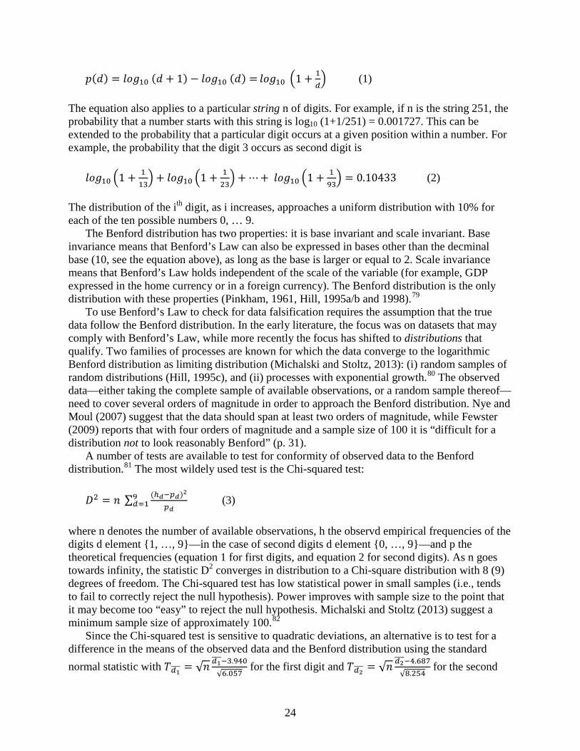
24

𝑝(𝑑) = 𝑙𝑜𝑔10 (𝑑 + 1) − 𝑙𝑜𝑔10 (𝑑) = 𝑙𝑜𝑔10 �1 + 1𝑑� (1)

The equation also applies to a particular string n of digits. For example, if n is the string 251, the probability that a number starts with this string is log10 (1+1/251) = 0.001727. This can be extended to the probability that a particular digit occurs at a given position within a number. For example, the probability that the digit 3 occurs as second digit is

𝑙𝑜𝑔10 �1 + 113� + 𝑙𝑜𝑔10 �1 + 1

23� + ⋯+ 𝑙𝑜𝑔10 �1 + 1

93� = 0.10433 (2)

The distribution of the ith digit, as i increases, approaches a uniform distribution with 10% for each of the ten possible numbers 0, … 9. The Benford distribution has two properties: it is base invariant and scale invariant. Base invariance means that Benford’s Law can also be expressed in bases other than the decminal base (10, see the equation above), as long as the base is larger or equal to 2. Scale invariance means that Benford’s Law holds independent of the scale of the variable (for example, GDP expressed in the home currency or in a foreign currency). The Benford distribution is the only distribution with these properties (Pinkham, 1961, Hill, 1995a/b and 1998).79 To use Benford’s Law to check for data falsification requires the assumption that the true data follow the Benford distribution. In the early literature, the focus was on datasets that may comply with Benford’s Law, while more recently the focus has shifted to distributions that qualify. Two families of processes are known for which the data converge to the logarithmic Benford distribution as limiting distribution (Michalski and Stoltz, 2013): (i) random samples of random distributions (Hill, 1995c), and (ii) processes with exponential growth.80 The observed data—either taking the complete sample of available observations, or a random sample thereof—need to cover several orders of magnitude in order to approach the Benford distribution. Nye and Moul (2007) suggest that the data should span at least two orders of magnitude, while Fewster (2009) reports that with four orders of magnitude and a sample size of 100 it is “difficult for a distribution not to look reasonably Benford” (p. 31). A number of tests are available to test for conformity of observed data to the Benford distribution.81 The most wildely used test is the Chi-squared test: 𝐷2 = 𝑛 ∑ (ℎ𝑑−𝑝𝑑)2

𝑝𝑑9𝑑=1 (3)

where n denotes the number of available observations, h the observd empirical frequencies of the digits d element {1, …, 9}—in the case of second digits d element {0, …, 9}—and p the theoretical frequencies (equation 1 for first digits, and equation 2 for second digits). As n goes towards infinity, the statistic D2 converges in distribution to a Chi-square distribution with 8 (9) degrees of freedom. The Chi-squared test has low statistical power in small samples (i.e., tends to fail to correctly reject the null hypothesis). Power improves with sample size to the point that it may become too “easy” to reject the null hypothesis. Michalski and Stoltz (2013) suggest a minimum sample size of approximately 100.82 Since the Chi-squared test is sensitive to quadratic deviations, an alternative is to test for a difference in the means of the observed data and the Benford distribution using the standard normal statistic with 𝑇𝑑1���� = √𝑛 𝑑1����−3.940

√6.057 for the first digit and 𝑇𝑑2���� = √𝑛 𝑑2����−4.687

√8.254 for the second

25

digit, where the mean of the first digit of the Benford distribution is 3.940 (with variance 6.057) and of the second digit 4.687 (with variance 8.254), and the mean of the observed first digits is obtained as 𝑑1��� = ∑ (𝑑19

𝑑1=1 + 0.5) ℎ𝑑1 and for the second digits 𝑑2��� = ∑ (𝑑29𝑑2=0 + 0.5) ℎ𝑑2.

The standard normal statistic can also be used to test for the compliance of individual digits with Benford’s Law, with a test statistic of 𝑇𝑑 = �𝑛𝑑

ℎ𝑑−𝑝𝑑�𝑝𝑑 (1−𝑝𝑑)

. Three further tests are the Kuiper test (a modified Kolmogorov-Smirnov test), the m (max) statistic and the d (distance) statistic. With Hd and Pd as the cumulative frequencies of the first digit d in the observed data and in the Benford distribution, the Kuiper statistic is 𝑇𝐾 =(𝐷𝑛+ + 𝐷𝑛−) [√𝑛 + 0.155 + 0.24

√𝑛], where 𝐷𝑛+ = sup[𝐻𝑑 − 𝑃𝑑] and 𝐷𝑛− = sup [𝑃𝑑 − 𝐻𝑑]. Leemis

et al. (2000) proposed the m statistic 𝑚 = max𝑑=1,…,9|ℎ𝑑 − 𝑝𝑑|, and Cho and Gaines (2007) the

d statistic 𝑑 = �∑ (ℎ𝑑9𝑑=1 −𝑝𝑑)2. Morrow (2010) provides Benford-specific test values at the 10,

5, and 1 percent significance level for the Kuiper test as well as for modified m and d tests, with the modification consisting of multiplication by √𝑛.83 Morrow notes that the small-n performance of these tests is fairly good in that the simulated test statistics are very close to the asymptotic values, especially for n≥80. Smith (1997) proposes a “Ones Scaling Test.” If one multiplies each number in the set by a constant, the distribution of first digits will remain unchanged as a consequence of the scale invariance of the Benford distribution (and only of the Benford distribution). He explores 696 multiplications by 1.01 (in the final instance this implies multiplication by 1000) and plots the fraction of numbers with digit one. If Benford’s Law is followed, the plot shows the same frequency in all 697 instances. Benford’s Law has been applied in a wide variety of circumstances. Of most interest in the context here are the applications to macroeconomic data series.84 For example, Rauch et al. (2011) examine annual national and financial accounts data (156 variables) for each EU country from 1999 to 2009 and rank countries by the adherence of their macroeconomic data to Benford’s Law (Greece’s data show the greatest deviation). Nye and Moul (2007) find that the World Bank International GDP data and the purchasing power parity corrected Penn World Table data for OECD countries conform well to Benford’s Law, but some subsets of the data, especially GDP data from the developing world, do not, suggesting deliberate manipulation of the underlying series. Michalski and Stoltz (2013) examine the quarterly balance of payments data of 103 countries in the period 1989 to 2007 to determine under which conditions (such as having a fixed exchange rate regime) countries’ data tend to violate Benford’s Law. Gonzalez-Garcia and Pastor (2009) examine five annual time series in each of the areas banking, balance of payments, national accounts, and government finance statistics for the period 1945-2007 for 80 countries (nested in six country groups) and find that most macroeconomic series for most country groups conform with Benford’s Law. Rejections of Benford’s Law, however, are not correlated with the corresponding data quality ratings compiled by experts based on the IMF’s Data Quality Assessment Framework (thus questioning the accuracy either of the expert opinions or of the Benford test). The authors also find that rejection of Benford’s Law may result from structural shifts in data series. Two authors show the importance of extending the analysis to the second digit. Diekmann (2007) in examining the first and second digits reported in published statistical estimates of research papers and in a similar set of faked data finds that both the first and second digits in published statistical estimates approximately match the Benford distribution, while only the first

26

digits of faked statistical estimates do. In the economic realm, Günnel and Tödter (2009) for forecasts of GDP growth and CPI inflation in Germany find that the second digits of forecasts exhibit an excess of zeros and fives. A key issue is how to interpret violations of Benford’s Law in the observed data. This could imply that the underlying data distribution violates Benford’s Law, that the data do not cover sufficient orders of magnitude, or that the data have been falsified.85 Rather than conclude on outright falsification, some of the literature proceeds to compare or rank different sets of data (such as different countries’ data on one and the same variable or set of variables) as to their conformity with Benford’s distribution. I.e., conformity to Benford’s Law is benchmarked against other comparable datasets; a lower degree of conformance is then interpreted as potentially lower data quality.86

5.2 Benford’s Law and Chinese National Income and Product Accounts Data

To examine Chinese national income and product accounts data, four sets of nominal data for the years 1978-2011 are selected:

• (production approach) GDP (with data as first published, and as most recently published); • sectoral VA for the four exhaustive sectors agriculture, industry, construction, and

services (with data as first published, and as most recently published); • aggregate expenditures; and • five exhaustive components of aggregate expenditures.

U.S. data on aggregate expenditures in their totatily, as well as with a breakdown into 8 and 14 components, are considered for comparison. (The U.S. does not publish production approach GDP data.) The number of observations for GDP or aggregate expenditures is small, with only 34 observations, and covering only two orders of magnitude. In the case of sectoral VA or the components of aggregate expenditures, the number of observations is above 100, typically covering three orders of magnitude. Table 6 reports the results of the test statistics introduced above: apart from the number of observations, it reports the significance levels (10, 5, and 1 percent) of any significant deviations of the actual data from the Benford distribution.87 As the top half of the table shows, the distributions of Chinese and U.S. nominal data do not differ significantly from the Benford distribution at the 10 percent significance level (except for two isolated instances), neither for first digits nor for second digits. Figure 10 provides the corresponding charts for a selection of nominal data. The bottom half of Table 6 reports the findings for the case of deflators and real growth rates for 1979-2011. With neither deflators nor real growth rates following an exponential distribution (and cumulative series being truncated from below at an arbitrary starting point, typically set at 100), only second digits of annual, non-cumulative deflators and real growth rates (expressed in percentages) are examined.88 First published real growth rates do not start until 1987 or 1990, depending on sector (using the real growth rate of a particular year as first published, and not using retrospectively constructed series for the early reform years). No official real growth data have been published for aggregate expenditures. Newly added are data for the high- and low-growth deflator scenario presented in the previous section. For the official data, deflators are (by necessity) implicit deflators, derived by dividing nominal growth rates by real growth rates. For

27

the high- and low-growth scenario, deflators are the ones constructed in the previous section, and real growth rates follow by applying the official nominal data. The U.S. separately publishes price and real growth data, with no such data available for the expenditure component ‘changes in inventories.’ The test statistics suggest that the sectoral high- and low-growth deflators constructed in the previous section do not follow the Benford distribution (though their aggregate does). Chinese official deflators (in the aggregate and by sector) follow the Bendford distribution, as do U.S. prices. It is for the real growth rates that test statistics consistently raise the alarm. Both, official Chinese real growth rates and U.S. real growth rates tend to not follow the Benford distribution. For China, the sectoral VA data fare better than the overall GDP data; for the U.S., aggregate expenditures in their totatily fare better than the data on expenditure components. Figure 11 presents a selection of the data (keeping in mind that the number of observations in the case of GDP is small and the statistical tests therefore accept large deviations). The figures show that for both the U.S. and China the problem with the real growth rates is that the second digit is zero with too high a frequency. This appears the only serious problem. The fact that there are too many zeros suggests rounding by the statistical authority, whether that is intentional, accurate rounding simply for the sake of rounding, or intentional, accurate rounding for the sake of not pretending a higher degree of accuracy than the data can provide, or intentional rounding for the sake of falsifying data.

6. Conclusions

Reviewing past and ongoing suspicions of the quality of Chinese GDP data, one is hard pressed to find evidence of data falsification. One may wonder if the 2006 benchmark revision following the 2004 economic census should not have led to higher real growth rates. One cannot but question the quality of the 2007 DRIE VA data (and then wonder how the NBS obtains data on industrial VA). And one may ponder if the 2007 real GDP growth rate is economically feasible. But there is no clear evidence of data falsification. The institutional arrangements of data compilation in China raise major questions. The NBS has no degree of formal independence and nobody makes any bones about the fact that the NBS serves the Party and the government. There is no transparency in how the NBS compiles data; how the NBS obtains the final nominal GDP value and real GDP growth rate is anybody’s guess. The limitations of publicly available data do not allow one to double-check the accuracy of the official (final) data. The NBS has scope for intentional manipulations in order to achieve a politically desirable GDP value or real GDP growth rate. The NBS can falsify nominal data, with implications for real growth rates, by falsifying data on that part of the economy on which it does not regularly publish data, such as small economic units that are covered through surveys only. It can also “falsify” nominal data by expanding its data compilation method and capturing an increasing share of the shadow economy. (To its credit, the NBS appears to have implemented such changes to its data compilation method in benchmark revisions that came with retrospective revisions to earlier data.) The NBS can falsify real growth rates through its choice of deflation method, as well as through its choice of retrospective revisions to nominal values and implicit deflators in benchmark revisions.

28

In the case of real growth rates, neither a double-check on the deflators of VA nor a double-check on the deflators of expenditure components yields significantly different aggregate (GDP) real growth rates. Plausible alternative deflators may yield up to one percentage point higher as well as lower average annual real growth rates for the reform period. That does not appear to be a clear bias, nor an exorbitant margin of error. The real growth rates are as good as the deflators and the aggregation methods are. The deflators are as good as the constant price method is or the individual price indices are; the individual price indices, in turn, depend on a vast array of individual price data collected. All deflation/aggregation methods come with inherent deficiencies, potentially giving too much weight to high-growth sectors due to high initial prices (leading to high growth rates), or neglecting quality change and thus causing deflators to be too high and growth rates to be too low. On balance, there is no clear overall effect. If the underlying individual price data, however, were incorrect, all bets on real growth rates are off. Chinese consumers will readily attest that China’s official CPI understimates true consumer price inflation—but so will European and American consumers for their respective CPIs. A test of Chinese statistics against Benford’s Law does not find any form of egregious data falsification. The only finding is that the second digit of real growth rates is ‘zero’ with too high a frequency—as is the case for the U.S. That does not rule out the very occasional data manipulation (which Benford’s Law cannot detect). In the end, one is left with an issue of trust: does one trust that the NBS in the many data manipulations that are needed to calculate GDP has no other purpose than to achieve an accurate estimate of GDP? Does the NBS simply work with large margins of error and an atrocious lack of transparency? Or is there an—Benford’s Law suggests at most occasional—political imperative that guides NBS manipulations of the underlying data? NBS explanations of how it obtains nominal VA and real growth rates are not encouraging as they appear at times inaccurate or contradictory, and the necessary data for double-checks data are not being made available. Things may not be much better in other countries. In the U.S., the Boskin Commission overnight changed real growth rates on grounds that may be perfectly plausible but only serve to illustrate the wide range of plausible inflation values, and thereby real growth values.89 In an economy with rapidly changing product characteristics and product variety, such as China, measuring inflation (and thereby real growth) accurately is potentially a challenging task. Political interference likewise is no anomaly: “President Lyndon Johnson would review the GNP reports before their release. If he did not like the report, he would keep sending the GNP estimates back to the Commerce Department until they got the numbers ‘correct.’” Under the first Bush administration, a senior member of the Executive Branch approached a large computer company with the request to in its report to the BEA exaggerate computer sales: “thanks to the heavy leverage of computer deflation, reported GDP growth enjoyed an artificial spike.”90 In contrast to the U.S., data falsification in China—if it occurs at the national level at all—may yet tread on lighter ground. In the final instance, when political regimes—in the East and in the West—derive their legitimacy from economic growth and when real GDP growth is difficult to measure accurately, reliable GDP figures may be an illusory commodity. When, furthermore, GDP by definition is an incomplete measure of productive activities and a flawed measure of well-being, perhaps it is time to de-emphasize the importance of GDP and to reflect on the ideological framework in which we operate.

29

References for China literature Bartholdy, Kasper. “Old and New Problems in the Estimation of National Accounts in Transition

Economies.” Economics of Transition 5, no. 1 (May 1997): 131-46. BAI Chong-en, and QIAN Zhenjie. “Guomin shouru de yaosu fenpei: tongji shuju beihou de

gushi” (Factor contribution: the story behind the numbers). Unpublished and undated manuscript, obtained December 2009.

BAI Chong-en, and QIAN Zhenjie. “The Factor Distribution in China: 1978-2007.” China Economic Review 21, no. 4 (Dec. 2010): 650-70.

BEA (Bureau of Economic Analysis). 2013. “2013 Comprehensive Revision of the National Income and Product Accounts,” at http://www.bea.gov/national/an1.htm#2013comprehensive (especially first item, “Briefing”), accessed 20 September 2013.

CAI Yongshun. “Between State and Peasant: Local Cadres and Statistical Reporting in Rural China.” The China Quarterly, no. 163 (Sept. 2000): 783-805.

China Infobank (at http://www.chinainfobank.com). “Yuce zhongguo ‘bu ke cesuan de jingji’ zhan GDP de bizhong yue wei 10%” (The ‘economic activities that cannot be estimated’ are estimated to be equivalent to 10% of GDP). 7 June 2003.

Chow, Gregory C. “Chinese Statistics.” The American Statistician 40, no. 3 (1986): 191-6. Economics Dictionary: Statistics. Jingji da cijian tongjijuan (Big Economics Dictionary,

Statistics Volume). Shanghai: Shanghai cishu chubanshe, 1996. Edin, Maria. “Why Do Chinese Local Cadres Promote Growth? Institutional Incentives and

Constraints of Local Cadres.” Forum for Development Studies, no. 1 (1998): 97-127. Fernald, John, Israel Malkin, and Mark Spiegel. “On the Reliability of Chinese Output Figures.”

FRBSF Economic Letter 2013-08, 25 March 2013, 5pp. Finance Ministry (General Office). Xianxing caiwu kuaiji zhidu quanshu (Complete current

financial accounting system). Two volumes. Beijing: Zhongguo caizheng jingji chubanshe, 1999.

GDP 1952-96. Zhongguo guonei shengchan zongzhi hesuan lishi ziliao (zhaiyao) (Historical Data on China’s Gross Domestic Product 1952-1995 (Summary)). Beijing: Zhongguo tongji chubanshe, 1998.

GUO Tan, and YI Xiaobo. “Zhongguo dixia jingji guimo jiben cesuan he shizheng fenxi” (Basic estimation of the size of China’s underground economy and a positive analysis). Gongye jishu jingji 25, no. 11 (Nov. 2006): 129-32.

Holz, Carsten. “‘Fast, Clear and Accurate:’ How Reliable Are Chinese Output and Economic Growth Statistics?” The China Quarterly, no. 173 (March 2003): 122-63.

_____. “Deconstructing China’s GDP Statistics.” China Economic Review 15, no. 2 (2004): 164-202.

_____. “China’s Reform Period Economic Growth: How Reliable Are Angus Maddison’s Estimates? Review of Income and Wealth 52, no. 1 (March 2006a): 85-119.

_____. “China’s Reform Period Economic Growth: How Reliable Are Angus Maddison’s Estimates? Response to Angus Maddison’s Reply.” Review of Income and Wealth 52, no. 3 (Sept. 2006b): 471-5.

_____. “Chinese Statistics: Classification Systems and Data Sources.” Stanford Center for International Development Working Paper No. 471, Stanford University, 8 January 2013(a).

30

_____. “Chinese Statistics: Output Data.” Stanford Center for International Development Working Paper No. 473, Stanford University, 1 March 2013(b).

_____. “Measuring Productivity Growth in China, 1952-2011.” Mimeo, Stanford Center for International Development. 2013(c).

Holz, Carsten A., and Yi-min Lin. “Pitfalls of China’s Industrial Statistics: Inconsistencies and Specification Problems.” The China Review 1, no. 1 (Fall 2001): 29-71.

Huenemann, Ralph W. “Are China’s Recent Transport Statistics Plausible?” China Economic Review 12, no. 4 (2001): 368-72.

Input-Output Tables 1997. Zhongguo touru chanchubiao 1997 (Input-Output Tables of China 1997). Beijing: Zhongguo tongji chubanshe, 1999.

Input-Output Tables 2007. Zhongguo touru chanchubiao 2007 (Input-Output Tables of China 2007). Beijing: Zhongguo tongji chubanshe, 2009.

Keidel, Albert. Keidel, Albert. “China’s GDP Expenditure Accounts.” China Economic Review 12, no. 4 (2001b): 355-67.

Klein, Lawrence, and Suleyman Ozmucur. “The Estimation of China’s Economic Growth Rate.” Journal of Economic and Social Measurement 28, no. 4 (2002-2003):187-202.

Koech, Janet, and Jian Wang. “China’s Slowdown May Be Worse Than Official Data Suggest.” Federal Reserve Bank of Dallas, Economic Letter 7, no. 8 (Aug. 2012): 1-4.)

Koen, Vincent. “Russian Macroeconomic Data: Existence, Access, Interpretation.” Communist Economies & Economic Transformation 8, no. 3 (Sept. 1996): 321-33.

Li Choh-Ming. The Statistical System of Communist China. Berkeley: University of California Press, 1962.

LIU Hua, ZHANG Weiwei, and LIAO Fugang. “Jiyu xianjin bilu moxing gaijin de wo guo dixia jingji guimo cesuan” (Estimate of the size of China’s underground economy based on an improved cash ratio model). Wuhan ligong daxue xuebao 29, no 1 (Jan. 2007): 138-40.

Maddison, Angus. Chinese Economic Performance in the Long Run. Paris: Development Centre of the Organisation for Economic Co-operation and Development, 1998.

Mehrotra, Aaron, and Pääkkönen. “Comparing China’s GDP Statistics with Coincident Indicators.” Journal of Comparative Economics 39 (2011): 406-11.

MENG Lian and WANG Xiaolu. “Dui zhongguo jingji zengzhang tongji shuju kexindu de guji” (An evaluation of the reliability of China’s statistics on economic growth). Jingji yanjiu, no. 10 (Oct. 2000): 3-13.

Movshuk, Oleksandr. “The Reliability of China’s Growth Figures: A Survey of Recent Statistical Controversies.” The Journal of Econometric Study of Northeast Asia 4, no. 1 (2002): 31-45.

NBS (National Bureau of Statistics). 1997. Zhongguo niandu guonei shengchan zongzhi jisuan fangfa (Calculation method of

China’s annual gross domestic product). NBS National Income Accounts Division. Beijing: Zhongguo tongji chubanshe. (This is one of seven small volumes explaining compilation practices of different NIPA statistics in China.)

2001. Zhongguo guonei shengchan zongzhi hesuan shouce (GDP accounting manual). No publishing house information or date; presumably an internal volume.

2003. Guojia tongji diaocha zhidu 2003 (National statistical survey system 2003). No publishing house information or date; presumably an internal volume.

2007. Zhongguo jingji pucha niandu guonei shengchan zongzhi hesuan fangfa (Calculation method of China’s annual gross domestic product from China’s economic census). NBS National Income Accounts Division. Beijing: Zhongguo tongji chubanshe, 2007.

31

2011. 2011 Guomin jingji hangye fenlei zhushi (2011 National sectoral classification scheme). Beijing: Zhongguo tongji chubanshe, 2011

NBS Industry and Transport Division. “Gongye zengzhang sudu zhong de ‘shuifen’ you duoda?” (How big is the ‘water content’ in industrial growth?), Jingji yanjiu cankao ziliao, no. 42 (19 March 1989): 2-5.

NBS Statistical Design and Administration Division. Guanyu tongji shang ruhe fanying suoyouzhi jiegou wenti de yanjiu (How to reflect the issue of ownership structure in the statistics). Beijing: Zhongguo tongji chubanshe, 1999.

NPC (National People’s Congress and its Standing Committee). 8 December 1983. “Zhonghua renmin gongheguo tongji fa” (PRC Statistics Law), in China

Infobank. 15 May 1996. “Zhonghua renmin gongheguo tongji fa” (PRC Statistics Law), revision of

original 8 December 1983 law, in China Infobank. 27 June 2009. “Zhonghua renmin gongheguo tongji fa” (PRC Statistics Law), revision of 15

May 1996 law. At http://www.npc.gov.cn/npc/xinwen/lfgz/zxfl/2009-06/27/content_1508548.htm, accessed 11 September 2009.

Orlik, Tom. Understanding China’s Economic Indicators:Translating the Data into Investment Opportunities. Upper Saddle River, NJ: FT Press Science, 2012.

Perkins, Dwight H. Market Control and Planning in Communist China. Cambridge, Massachusetts: Harvard University Press: 1966. Appendix A: Reliability of Chinese Statistics (pp. 215-25).

Powers, Susan. “Statistical Needs in Eastern Europe,” Monthly Labor Review 115, no. 3 (March 1992): 18-28.

Population Census 2010. Zhongguo 2010 nian renkou pucha ziliao (Materials on China’s 2010 Population Census). Three volumes, compiled by the population census office under the State Council and the NBS Department of Population and Employment Statistics. Beijing: Zhongguo tongji chubanshe, 2012.

Rawski, Thomas G. “On the reliability of Chinese economic data: discussion.” Journal of Development Studies 12, no. 4 (1976): 438-41.

_____. “China by the Numbers: How Reform Has Affected China’s Economic Statistics.” China Perspectives, no. 33 (Jan./Feb. 2001): 25-34.

Rawski, Thomas G., and XIAO Wei. “China Economic Review Symposium on Chinese Economic Statistics: Introduction.” China Economic Review 12, no. 4 (2001): 298-302.

Schneider, Friedrich, and Dominik H. Enste. “Shadow Economies: Size, Causes, and Consequences.” Journal of Economic Literature 38, no. 1 (March 2000): 77-114.

Sinclair, Tara M. “Characteristics and Implications of Chinese Macroeconomic Data Revisions.” Mimeo, Department of Economics and Elliott School for International Affairs, The George Washington University, 21August 2012.

Wu, Harry X. “The Chinese GDP Growth Rate Puzzle: How Fast Has the Chinese Economy Grown?” Asian Economic Papers 6, no. 1 (Winter 2007): 1-23.

Xia Xingyuan and Wan Anpei. Zhongguo dixia jingji wenti yanjiu (Study of China’s Underground Economy). Zhengzhou: Henan renmin chubanshe, 1993.

XU Xianchun. “Shijie yinhang gaogu zhongguo GDP shuju” (The World Bank overestimates China’s GDP). Zhongguo guoqing guoli, no. 1 (1999a): 7-10.

32

_____. “Shijie yinhang dui zhongguo guanfang GDP shuju de tiaozheng he chongxin renke” (The official Chinese GDP figures as adjusted and approved by the World Bank). Jingji yanjiu, no. 6 (June 1999b): 52-8.

_____. “Zhongguo guonei shengchan zongzhi hesuan zhong cunzai de ruogan wenti yanjiu” (Some problems in the calculation of China’s GDP). Jingji yanjiu, no. 2 (Feb. 2000a): 10-16.

_____. Zhongguo guonei shengchan zongzhi hesuan (Calculation of China’s GDP). Beijing: Beijing daxue chubanshe, 2000(b).

_____. “Woguo GDP hesuan yu xianxing SNA de GDP hesuan zhijian de ruogan chayi” (Some discrepancies in China’s GDP compilation in comparison to the current SNA GDP compilation methods). Jingji yanjiu, no. 11 (Nov. 2001): 63-8.

_____. “Study on Some Problems in Estimating China’s Gross Domestic Product.” Review of Income and Wealth 48, no. 2 (June 2002): 205-15.

_____. “Guanyu jingji pucha niandu GDP hesuan de bianhua” (Changes in the calculation of annual GDP in the economic census). Jingji yanjiu, no. 2 (February), 2006: 16-20.

_____. “The Establishment, Reform, and Development of China’s System of National Accounts.” Review of Income and Wealth 55, special issue 1 (July 2009): 442-65.

YANG Jisheng. Tombstone: The Great Chinese Famine, 1958-1962. New York: Farrar, Straus and Giroux, 2012.

Young, Alwyn. “Gold into Base Metals: Productivity Growth in the People’s Republic of China During the Reform Period.” NBER Working Paper Series 7856, August 2000.

ZHANG Sai. “Guanyu ‘Zhonghua renmin gongheguo tongjifa xiuzhengan (zao’an)’ de shuoming” (Explanation of the (draft) scheduled revisions to the PRC Statistics Law). 23 August 1995. In China Infobank.

ZHANG Zhichao, DING Hong, and DAN Fangfang. “Zhongguo dixia jingji de guimo guce” (An estimate of the size of China’s underground economy). Lilun xintan, no. 12 (2004): 22f.

ZHAO Peng. “Nongcun jingji tongji bu shi de yuanyin ji duice” (Reasons why rural statistics are false and counter-policies). Nongcun Hezuo Jingji Jingying Guanli, no. 6 (1998): 42f.

References for literature on Benford’s Law Benford, Frank. “The Law of Anomalous Numbers.” Proceedings of the American Philosophical

Society 78, no. 4 (31 March 1938): 551-72. Browne, Malcom. W. “Following Benford’s Law, or Looking Out for No. 1.” At

http://www.rexswain.com/benford.html, last accessed 15 January 2013. Cho, Wendy K. Tam, and Brian J. Gaines. “Breaking the (Benford) Law.” The American

Statistician 61, no. 3 (August 2007): 218-23. Deckert, Joseph, Mikhail Myagkov, and Peter C. Ordeshook. “Benford’s Law and the Detection

of Election Fraud.” Political Analysis 19, no. 3 (2011): 235-68. Diekmann, Andreas. “Not the First Digit! Using Benford’s Law to Detect Fraudulent Scientific

Data.” Journal of Applied Statistics 34, no. 3 (April 2007): 321-9. Durtschi, Cindy, William Hillison, and Carl Pacini. “The Effective Use of Benford’s Law to

Assist in Detecting Fraud in Accounting Data.” Journal of Forensic Accounting V, no 1 (2004): 17-34.

el Sehity, Tarek, Erik Hoelzl, and Erich Kirchler. “Price Developments after a Nominal Shock: Benford’s Law and Psychological Pricing after the Euro Introduction.” International Journal of Research in Marketing 22, no. 4 (December 2005): 471-80.

33

Fewster, R.M. “A Simple Explanatoin of Benford’s Law.” The American Statistican 63, no. 1 (2009): 26-32.

Giles, David E. “Benford’s Law and Naturally Occurring Prices in Certain ebaY Auctions.” Applied Economics Letters 14, no. 3 (2007): 157-61.

Gonzalez-Garcia, Jesus, and Gonzalo Pastor. “Benford’s Law and Macroeconomic Data Quality.” IMF Working Paper WP/09/10 (January 2009).

Günnel, Stefan, and Karl-Heinz Tödter. “Does Benford’s Law Hold in Economic Research and Forecasting?” Empirica 36, no. 3 (August 2009): 273-92.

Hill, Theodore P. “Base-Invariance Implies Benford’s Law.” Proceedings of the American Mathematical Society 123, no. 3 (March 1995a): 887-95.

_____. “The Significant-Digit Phenomenon.” The American Mathematical Monthly 102, no. 4 (April 1995b): 322-7.

_____“A Statistical Derivation of the Significant-Digit Law.” Statistical Science 10, no. 4 (Nov. 1995c): 354-63.

_____. “The First Digit Phenomenon: A Century-old Observation about an Unexpected Pattern in Many Numerical Tables Applies to the Stock Market, Census Statistics and Accounting Data.” American Scientist 86, no. 4 (July-August 1998): 358-63.

Judge, George, and Laura Schechter. “Detecing Problems in Survey Data Using Benford’s Law.” The Journal of Human Resources 44, no. 1 (Winter 2009): 1-24.

Leemis, Lawrence M., Bruce W. Schmeiser, and Diane L. Evans. “Survival Distributions Satisfying Benford’s Law.” The American Statistician 54, no. 4 (November 2000): 236-41.

Michalski, Tomasz, and Gilles Stoltz. “Do Countries Falsify Economic Data Strategically? Some Evidence That They Might.” Review of Economics and Statistics 95, no. 2 (May 2013): 591-616.

Morrow, John. “Benford’s Law, Families of Distributions and a Test Basis.” Mimeo, 9 October 2010.

Newcomb, Simon. “Note on the Frequence of Use of the Different Digits in Natural Numbers.” American Journal of Mathematics 4, no. 1/4 (1881): 39-40.

Nigrini, Mark J. “A Taxpayer Compliance Application of Benford’s Law.” Journal of the American Taxation Association 18, no. 1 (Spring 1996): 72-91.

_____. Benford’s Law: Applications for Forensic Accounting, Auditing, and Fraud Detection. Hoboken, N.J.: John Wiley & Sons, 2012.

Nye, John, and Charles Moul. “The Political Economy of Numbers: On the Application of Benford’s Law to International Macroeconomic Statistics.” The B.E. Journal of Macroeconomics 7, no. 1, Article 17 (July 2007), 14pp.

Pinkham, Roger S. “On the Distribution of First Significant Digits.” The Annals of Mathematical Statistics 32, no. 4 (December 1961): 1223-30.

Raimi, Ralph A. “On the Distribution of First Significant Figures.” The American Mathematical Monthly 76, no. 4 (April 1969): 342-8.

_____. “The First Digit Problem.” The American Mathematical Monthly 83, no. 7 (August-September 1976): 521-38.

Rauch, Bernhard, Max Göttsche, and Gernot Brähler. “Fact and Fiction in EU-Governmental Economic Data.” German Economic Review 12, no. 3 (August 2011): 243-55.

Smith, Steven W. “Explaining Benford’s Law.” Chapter 34 in The Scientist and Engineer’s Guide to Digital Signal Processing. Available at http://www.dspguide.com/ch34.htm, last accessed 24 October 2013. (Hardcover publication date: 1997.)

34

Stephens, M.A. “Use of the Kolmogorov-Smirnov, Cramér-Von Mises and Related Statistics without Extensive Tables.” Journal of the Royal Statistical Society 32, Series B (Methodological), no. 1 (1970): 115-22.

Thomas, Jacob K. “Unusual Patterns in Reported Earnings.” The Accounting Review 64, no. 4 (October 1989): 773-87.

Varian, Hal R. “Benford’s Law” (in section “Letters to the Editor). The American Statistician 26, no. 3 (June 1972): 65f.

Weisstein, Eric W. “Benford’s Law.” At http://mathworld.wolfram.com/BenfordsLaw.html, last accessed 14 January 2013.

35

Table 1. Annual Rebisions to National Value-Added, Real GDP Growth Rates

Nominal: Annual revised value / first published value Real GDP growth rates (in %) Official values Constructed Total

(GDP) Primary sector

Secondary sector

# Ind.

# Constr.

Tertiary sector

As first published

Statistical Yearbook

Törn-qvist

2005 2012 index 1987 10.4 / 11.1 11.6 11.6 10.9 1988 10.4 / 11.2 11.3 11.3 11.7 1989 3.5 / 4.3 4.1 4.1 3.3 1990 5.0 / 3.9 3.8 3.8 3.9 1991 7.8 / 8.0 9.2 9.2 12.4 1992 13.2 14.2 14.2 17.6 17.8 1993 1.104 1.035 1.011 1.000 1.085 1.335 13.4 13.5 14.0 15.5 15.8 1994 1.039 1.002 1.052 1.055 1.039 1.043 11.8 12.6 13.1 17.0 17.0 1995 1.004 1.000 1.013 1.015 1.000 0.992 10.5 10.5 10.9 11.6 11.4 1996 0.990 0.997 1.000 1.000 1.000 0.968 9.6 9.6 10.0 9.4 9.1 1997 0.996 1.017 1.012 1.021 0.959 0.958 8.8 8.8 9.3 9.6 9.1 1998 0.987 0.997 0.998 0.999 0.994 0.964 7.8 7.8 7.8 8.1 7.6 1999 1.002 1.001 1.004 1.003 1.005 1.000 7.1 7.1 7.6 8.9 8.6 2000 1.001 1.029 0.988 0.987 0.995 1.007 8.0 8.0 8.4 9.6 9.4 2001 1.014 1.055 0.993 0.995 0.987 1.028 7.3 7.5 8.3 10.5 10.6 2002 1.004 1.000 0.990 0.988 1.000 1.027 8.0 8.3 9.1 10.1 10.2 2003 1.001 0.990 1.000 1.000 1.000 1.008 9.3 9.5 10.0 10.7 10.9 2004 1.168 1.009 1.021 1.038 0.908 1.487 9.5 9.5 10.1 10.5 11.0 2005 1.004 1.000 1.004 1.004 1.000 1.006 10.2 11.3 11.3 11.4 2006 1.005 0.972 1.000 1.000 1.000 1.021 11.1 12.7 13.3 13.4 2007 1.031 1.019 1.028 1.030 1.018 1.038 11.9 14.2 16.8 16.9 2008 1.044 0.991 1.019 1.009 1.098 1.090 9.0 9.6 10.2 10.2 2009 1.001 1.000 1.000 1.000 1.000 1.003 9.1 9.2 9.2 9.2 2010 1.001 1.000 0.999 0.999 0.998 1.003 10.4 10.4 10.5 10.4 2011 9.3 9.3 9.3 9.3

All ratios of annual revisions through 2003 are obtained as national value published in the Statistical Yearbook 2005 divided by the national value as first published in the then current year Statistical Yearbook. After 2003, all data are the second-most recent year’s value in a Statistical Yearbook issue divided by the most recent value in the previous issue. Year 1993 GDP was retrospectively revised upward largely because of a 33.45 percent upward revision to tertiary sector VA following the 1993 tertiary sector census. Tertiary sector VA was first revised in the Statistical Yearbook 1995, and then a second time (which is unusual), by a minor amount, in the Statistical Yearbook 1996. 2004 and 2008 are economic census years As first published: individual issues of the Statistical Yearbook series. The starting year is 1987 because the Statistical Yearbook 1988 (with most recent data for 1987) is the first issue with GDP data. For 1987-1991, GDP data are not available: the first figure represents the weighted average of the real growth rates of the three main economic sectors (using previous-year nominal values as weights), the second figure is the one published retrospectively in the Statistical Yearbook 1993, pp. 31f. Constructed series: first published implicit deflator, Statistical Yearbook 2012 nominal values. To compile the Törnqvist index, the nominal growth rates of the three main economic sectors are divided by the corresponding first published implicit deflators; the resulting sectoral real growth rates are then aggregated into real GDP growth rates using a Törnqvist index with the nominal shares as weights.

36

Sources: first published values from Statistical Yearbook 1995 (pp. 32, 36) for all years through 1994, and then each subsequent year’s Statistical Yearbook. (Aggregate expenditure data became available in the Statistical Yearbook 1995 only, with data from 1978 onwards. This source does not report VA values of 1979 and 1981-83, but the Statistical Yearbook 1998, p. 55, does, with identical production approach values for 1978, 1980, and 1984 as in the Statistical Yearbook 1995).

Figure 1. Nominal GDP Divided by Aggregate Expenditures

0.94

0.95

0.96

0.97

0.98

0.99

1.00

1.01

1.02

1.03

1.04

1978 1981 1984 1987 1990 1993 1996 1999 2002 2005 2008 2011

First published

Statistical Yearbook 2012

37

Table 2. Summed Provincial Value-Added Divided by GDP

Total (GDP)

Primary sector

Secondary sector

# Industry

# Construction

Tertiary sector

1991 0.969 1.002 0.982 0.977 1.024 0.918 1992 0.983 0.998 0.983 0.977 1.025 0.972 1993a 1.091 1.028 1.004 1.001 1.019 1.307 1994 1.013 0.982 1.013 1.024 0.946 1.019 1995 0.989 0.996 0.957 n.a. n.a. 1.034 1996 1.000 1.004 0.950 0.960 0.886 1.077 1997 1.029 1.047 0.981 0.994 0.898 1.093 1998 1.043 1.018 0.997 0.998 0.994 1.123 1999 1.070 1.011 1.008 1.003 1.043 1.194 2000 1.087 1.044 1.007 0.998 1.065 1.232 2001 1.113 1.064 1.016 1.005 1.087 1.283 2002 1.126 1.006 1.038 1.023 1.139 1.316 2003 1.156 1.005 1.084 1.069 1.178 1.336 2004 1.193 1.006 1.139 1.128 1.213 1.370 2005 1.080 0.997 1.113 1.111 1.135 1.067 2006 1.096 1.000 1.121 1.123 1.103 1.093 2007 1.105 1.017 1.140 1.149 1.070 1.087 2008 1.088 0.993 1.142 1.154 1.048 1.051 2009 1.073 1.000 1.141 1.165 1.000 1.017 2010 1.089 1.000 1.173 1.202 1.001 1.019 2011 1.103 0.999 1.197 1.230 1.000 1.025

Data are first published values, in the Statistical Yearbook of the year following the year covered by the data, with the provincial data until (including) 1994 first published in the Statistical Yearbook of two years later. (1995 provincial values are taken from GDP 1952-96.) a The 1993 provincial values are the first published values, available in the Statistical Yearbook 1995, incorporating the findings of the tertiary sector census of 1993. The 1993 national value is the first published value, available in the Statistical Yearbook 1994, not incorporating the findings of the tertiary sector census of 1993. (2004 and 2008 values are pre-economic census values, for provincial and national data.)

38

The period covered is 1978-1997. The countries constitute a selection of highly developed countries and of developing countries in Latin America, Europe, and Asia. All transition countries for which product quantity data are available in the two years (1978 and 1995) are included. The country selection was made prior to any calculations. The period through 1997 is chosen because Wu (2002), in an early version of which Maddison’s work is based, conducts his analysis through 1997. The product quantity data are from the United Nations Industrial Commodity Production Statistics Database (http://unstats.un.org/unsd/snaama, accessed on 10 Oct. 04, with industrial VA of Taiwan in constant prices from http://www.stat.gov.tw/bs4/nis/enisd.htm, accessed on 9 Feb. 2004).) For each country, all products on which data are available are used. The number of products varies from 17 in the case of Taiwan to 129 in the case of China and 380 in the case of Japan.

Figure 2. Average Annual Growth Rates of Product Quantities Vs. Real Value-Added

-2-10123456789

101112

-6 -5 -4 -3 -2 -1 0 1 2 3 4 5 6 7 8 9 10 11 12

Indu

stria

l gro

ss v

alue

add

ed

Product quantities

China

Indonesia

Thailand

Romania

Bulgaria Poland

Malaysia Korea

Taiwan Vietnam Ireland

Turkey

India

USA

UK

Mexico Japan Portugal

Argentina Brazil

45-degree line

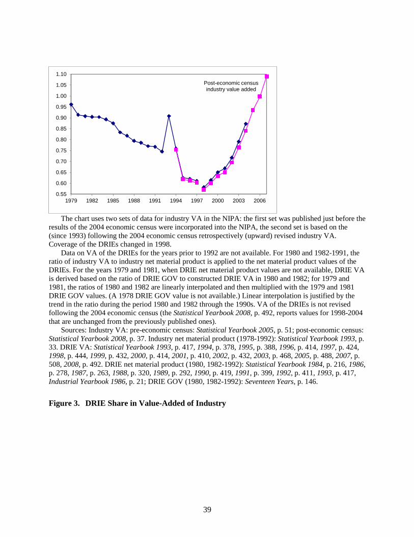
39

The chart uses two sets of data for industry VA in the NIPA: the first set was published just before the results of the 2004 economic census were incorporated into the NIPA, the second set is based on the (since 1993) following the 2004 economic census retrospectively (upward) revised industry VA. Coverage of the DRIEs changed in 1998. Data on VA of the DRIEs for the years prior to 1992 are not available. For 1980 and 1982-1991, the ratio of industry VA to industry net material product is applied to the net material product values of the DRIEs. For the years 1979 and 1981, when DRIE net material product values are not available, DRIE VA is derived based on the ratio of DRIE GOV to constructed DRIE VA in 1980 and 1982; for 1979 and 1981, the ratios of 1980 and 1982 are linearly interpolated and then multiplied with the 1979 and 1981 DRIE GOV values. (A 1978 DRIE GOV value is not available.) Linear interpolation is justified by the trend in the ratio during the period 1980 and 1982 through the 1990s. VA of the DRIEs is not revised following the 2004 economic census (the Statistical Yearbook 2008, p. 492, reports values for 1998-2004 that are unchanged from the previously published ones). Sources: Industry VA: pre-economic census: Statistical Yearbook 2005, p. 51; post-economic census: Statistical Yearbook 2008, p. 37. Industry net material product (1978-1992): Statistical Yearbook 1993, p. 33. DRIE VA: Statistical Yearbook 1993, p. 417, 1994, p. 378, 1995, p. 388, 1996, p. 414, 1997, p. 424, 1998, p. 444, 1999, p. 432, 2000, p. 414, 2001, p. 410, 2002, p. 432, 2003, p. 468, 2005, p. 488, 2007, p. 508, 2008, p. 492. DRIE net material product (1980, 1982-1992): Statistical Yearbook 1984, p. 216, 1986, p. 278, 1987, p. 263, 1988, p. 320, 1989, p. 292, 1990, p. 419, 1991, p. 399, 1992, p. 411, 1993, p. 417, Industrial Yearbook 1986, p. 21; DRIE GOV (1980, 1982-1992): Seventeen Years, p. 146.

Figure 3. DRIE Share in Value-Added of Industry

0.55

0.60

0.65

0.70

0.75

0.80

0.85

0.90

0.95

1.00

1.05

1.10

1979 1982 1985 1988 1991 1994 1997 2000 2003 2006

Post-economic census industry value added

40

All values are mid-year values. Industry employment: secondary sector employment times the share of industry in secondary sector employment. Secondary sector employment values of the years prior to 1990 are adjusted (see Holz, 2013c). Values for the share of industry in secondary sector employment are available from the population censuses (1982, 1990, 2000, and 2010) and population surveys (1987, 1995, 2005). Share values of other years are interpolated; identical annual growth rates are assumed for all years between two adjacent census/survey dates. The census and survey values for the years through 1990 are of 1 July, and since then of 1 November of that year. The census value of 1 November 1995 was adjusted to turn it into a 1 July 1995 value. To obtain annual values for the years since 1996, the annual growth rate from 1 November in the first year of the interval to 1 November in the last year of the interval was applied to each year’s 1 July value (in this interval). Employment values for the DRIEs are “average annual total employment” in 1994-2011, with the values for 1994-1997 obtained as DRIE VA divided by (published) DRIE labor productivity (which yields an identical value to the published average annual total employment value for 1998, the first year for which this particular employment series is published). For the years prior to 1994, DRIE employment values are “average annual staff and workers,” in the one overlapping year 1993 identical up to a difference of 0.0006 percent to the “average annual total employment.” Coverage of the DRIEs changed significantly in 1998 and in 2011. Sources: Secondary sector employment: Statistical Yearbook 2012, p 128. Shares of industry in secondary sector employment: Population Census and Population Survey volumes of the corresponding years. DRIE employment: 1998-2011: Statistical Yearbook 2012, p. 510; 1994-1998: Statistical Yearbook 1995, pp. 385, 401, 1996, pp. 411, 427, 1997, pp. 414, 437, 1998, 444, 459, 1999, 432, 437 (labor productivity and VA); 1978-1994 (as available): Industrial Statistical Yearbook 1993, p. 90, 1994, p. 81, 1995, p. 79.

Figure 4. DRIE Share in Industry Employment

0.38

0.43

0.48

0.53

0.58

0.63

0.68

1978 1981 1984 1987 1990 1993 1996 1999 2002 2005 2008 2011

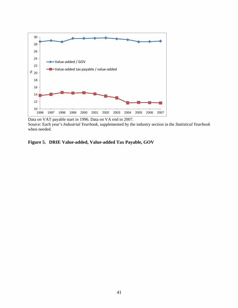
41

Data on VAT payable start in 1996. Data on VA end in 2007. Source: Each year’s Industrial Yearbook, supplemented by the industry section in the Statistical Yearbook when needed.

Figure 5. DRIE Value-added, Value-added Tax Payable, GOV

10

12

14

16

18

20

22

24

26

28

30

1996 1997 1998 1999 2000 2001 2002 2003 2004 2005 2006 2007

%

Value-added / GOV

Value-added tax payable / value-added

42

Table 3. Reliability of GDP Data Compilation Methods (2000)

Two groups?a

Approach to calculating value-added

Need data from

Data sources other than direct

Share of this sector

Share in % of sector (sub-sector) value-added that isd

(“Direct” vs.

“indirect”)

Produc-tion

approach

Income approach

“direct” for “indirect”

group?

reporting (where mentioned)

in GDP, year 2000,

in %

highly reliable

some-what

reliable

unreliable

Farming, forestry, husbandry, fisheries Yes 16.35 100.00 Industry Yes For direct For indirectc Survey 43.66 66.49 33.51 Construction Yes (Yesb) (Yesb) Yes 6.58 56.74 43.26 Tertiary sector 33.41 Transport (and storage), post and

telecommunications Yes Theore-

ticallyb For direct; indirectc

Both approaches

(6.05) 60.00 40.00

Wholesale/ retail trade, catering Yes (Yes) For direct; indirectc

Production approach

Survey, tertiary census, I/O table

(8.18) 48.62 51.38

Banking and insurance (5.83) 80.00 20.00 Banking Yes (Yes) Yesc Both appr. Insurance (Yes) Yes

Real estate (Yesb) Yes Survey (1.86) 100.00 Government, Party, social organizations Yes I/O table (2.62) 100.00 All other services Yes Tertiary census,

I/O table (8.87) 50.00 50.00

Services for farming, etc. [0.26] Geological prospecting, water cons. [0.37] Social services [3.63] Health care, sports, social welfare [0.92] Educ., culture, arts, radio, film, TV [2.67] Scientific research, polytechnic serv. [0.70] Others [0.31]

Total: share in GDP, 2000, in % 45.03 11.07 43.90 A “Yes” in parenthesis means that this approach is not the main approach. The 2000 (pre-economic census) GDP value is 8,944.22b yuan. Statistical Yearbook 2002, p. 51. a Are the production units in this sector (or subsector) split into two groups, i.e., units reporting directly to the statistics xitong or some other government department vs. units not reporting directly? The directly reporting units carry labels such as “above-norm enterprises” or “designated units,” with the definitions being sector-specific.

43

b The source describes how the production approach is used in this sector (subsector), but describes only the calculation of GOV. It then mentions that VA is obtained through the income approach, and GOV minus income approach VA yields the value of intermediate inputs. In the case of construction, VA of those units not reporting directly to the statistics xitong are based on GOV and investment statistics combined with VA ratios obtained from the group of directly reporting units (where VA was obtained using the income approach). c In the calculation of the VA of the “indirect” group in industry, income approach VA is obtained through sampling, with the ratio of (income approach) VA to GOV in the sample then applied to the GOV “estimated” for the whole group of enterprises not reporting directly to the statistics xitong or government departments. In the case of transport, post and telecommunications, for some units within the “indirect” group the income approach is supported with ratios obtained from the “direct” group, while for other units, GOV is obtained and then multiplied by the ratio of VA to GOV in the “direct” group. In wholesale/retail trade and catering, a ratio of VA to GOV is obtained from the last tertiary sector census or the latest input-output table and then applied to the GOV of the “indirect” group. For approximately 80 percent of the banking sector (measured in terms of loans), data on income approach VA are available; ratios obtained from this group are then applied to total loans. d The categorization of data as highly reliable, somewhat reliable, or unreliable is subjective. In industry and construction, the split into two groups is based on the share of sectoral VA produced in directly reporting (“above-norm”) units. No data on transportation, post and telecommunications occurring outside the xitong are available (apart from aggregate sectoral VA); in waterway and highway transportation this share may be high. In wholesale/retail trade and catering, the split into two groups was based on the share of sales units “above designated size” (directly reporting units). In banking and insurance, the split into two groups was based on the share in total loans of those banks on which the NBS has balance sheet and profit and loss account data available (to derive income approach VA). Sources: Xu (2000b), NBS (1997a). Statistical Yearbook 2001, pp. 410, 465f., 551, 559; 2002, pp. 51, 55.

44

RPI: retail price index. PPI: producer price index for farm products. For details see Appendix A.

Figure 6. Primary Sector Deflators

For details see Appendix A.

Figure 7. Industry Deflators

85

95

105

115

125

135

145

Implicit deflator (2012 publication)Rural RPIRural RPI, double-defl. by sector, one intermediate input price1978-2000: agric. proc. prices; 2001: implicit defl.; 2002-: agric. PPI

95

100

105

110

115

120

125 Implicit deflator, 2012publication

Implicit deflator, as firstpublished

PPI (Ex-factory priceindex of ind. products)

45

For details see Appendix A.

Figure 8. Tertiary Sector Deflators

85

90

95

100

105

110

115

120

125

Implicit deflator, 2012 publication

Implicit deflator, as first published

Tornqvist index, 6 sub-sectors, official deflators

Tornqvist index, 6 sub-sectors, approximated deflators

46

Table 4. Average Annual Real GDP Growth Rates

Implicit deflator: Reasonable deflator scenario for Statistical

Yearbook 2012

“official”

As first pub-lished (1987/ 90-, earlier

years: official)

high real growth low real growth

Primary sector Rural RPI Rural RPI, double-deflated by sector, one intermediate input price

Industry As first published PPI Construction Investment in fixed assets

price index: construction and installation sub-index (-1990: official)

Industrial products purchasing price index: building materials sub-index (-1988: official)

Tertiary sector As first published Törnqvist index of approx.. deflators for exhaustive six tertiary sector sub-sectors

Average annual real GDP growth rate 1978-2011, in % 9.8 10.5 11.0 9.1

For details see Appendix A.

Figure 9. Alternative GDP Deflators

95

100

105

110

115

120

125

130 Official deflators(2012 publication)Deflators as firstpublishedApprox. high-real-growth deflatorsApprox. low-real-growth deflators

47

Table 5. Average Annual Real Growth Rates of Aggregate Expenditures

Semi-official Constructed A Constructed B Reference: as

Törnqvist index

as Törnqvist

index

as Törnqvist

index

GDP

1983-2004 9.9 9.9 9.4 9.4 9.5 9.5 10.0 1979-2004 9.6 9.6 9.2 9.2 9.3 9.3 9.6 1979-2011 10.0 10.0 10.1 10.1 9.9 1983-2011 10.3 10.3 10.3 10.3 10.2 For definitions of the three (six) series see the text. The data for the reference GDP series are the official real growth rates reported in the Statistical Yearbook 2012.

48

Table 6. Significance Levels of Deviations of Actual Data from the Benford Distribution

Nominal data 𝐷2 𝑇𝑑� 𝑇𝑑 𝑇𝐾 m* d* 𝐷2 𝑇𝑑� 𝑇𝑑 𝑇𝐾 m* d* n First digit Second digit China GDP as first published 34 GDP (Statistical Yearbook 2012) 34 Sectoral VA (4 sectors) as first published 136 5 Sectoral VA (4 sectors) (Statistical Yearbook 2012) 136 10 Aggregate expenditures (Statistical Yearbook 2012) 34 Aggregate expenditures: 5 components (Statistical Yearbook 2012) 170 U.S. Aggregate expenditures 34 Aggregate expenditures: 8 components 272 Aggregate expenditures: 14 components 476 Deflators and real growth rates: second digit 𝐷2 𝑇𝑑� 𝑇𝑑 𝑇𝐾 m* d* 𝐷2 𝑇𝑑� 𝑇𝑑 𝑇𝐾 m* d* n Deflators Real growth rates China (implicit deflators, published real growth rates) GDP as first published 25 1 1 a 1 1 1 GDP (Statistical Yearbook 2012) 33 10 5 1 c 5 10 10 GDP constructed high-growth scenario 33 10 10 GDP constructed low-growth scenario 33 10 Sectoral VA (4 sectors) as first published 94 1 10 5 5 Sectoral VA (4 sectors) (Statistical Yearbook 2012) 132 10 5 Sectoral VA (4 sectors) constructed high-growth scenario 132 1 b 1 1 1 Sectoral VA (4 sectors) constructed low-growth scenario 132 5 5 10 10 U.S. Aggregate expenditures 33 10 10 Aggregate expenditures: 7 components 231 5 5 5 5 Aggregate expenditures: 13 components 429 5 5 c 5 1 5 No entry implies no significance at the 10% level. For both China and the U.S., nominal values cover the years 1978-2011, while deflators and real growth rates cover the years 1979-2011.

Exceptionally, Chinese first published implicit deflators and real growth rates in agriculture and services cover the years 1987-2011, and in industry and construction 1990-2011; those of GDP cover the years 1987-2011 with real growth rates of 1987-1991 constructed from sectoral real growth rates (primary-agriculture, secondary, and tertiary-service sector) using previous-year nominal weights.

49

n: Number of observations. Test statistics: 𝐷2: Chi-squared statistic. 𝑇𝑑�: Difference in means standard normal statistic (two-sided test). 𝑇𝑑: Difference in individual digits

(specific digit in actual vs. Benford distribution) standard normal statistic (two-sided test). 𝑇𝐾: Kuiper statistic. m*: Modified Leemis et al. (2000) m-statistic (m-statistic times √𝑛). d*: Modified Cho and Gaines (2007) d-statistic (d-statistic times √𝑛).

China GDP as first published: GDP through 1991 obtained as summed sectoral VA; values through 1987 from Statistical Yearbook 1988 (the first source of such data).

China sectoral VA (4 sectors): GDP breakdown into the four exhaustive sectors agriculture, industry, construction, and services. China aggregate expenditures: 5 exhaustive components: household consumption, government consumption, gross fixed capital formation,

inventory change (always positive and larger than ten units (100m yuan RMB)), and absolute values of net exports times 100. U.S. aggregate expenditures: 8 (7) exhaustive components: personal consumption of goods, personal consumption of services, fixed gross private

domestic investment, absolute value of change in private inventories (in gross private domestic investment) times 100 [no deflator and real growth rate values available], exports, imports, federal government consumption and gross investment, state and local government consumption and gross investment.

U.S. aggregate expenditures: 14 (13) exhaustive components: in personal consumption: durable goods, non-durable goods, services; in gross private domestic investment: non-residential structures, non-residential equipment and software, residential, absolute value of change in private inventories times 100 [no deflator and real growth rate values available]; in exports: goods, services; in imports: goods, services; in government consumption expenditures and gross investment: federal national defense, federal non-defense, state and local.

GDP constructed high-/low-growth scenario refers to the deflators and real growth rates constructed for these scenarios in the previous section. Note a (b, c): second digit 0 at 1% (5%, 10%) significance level. (In all cases, the digit 0 has more observations than the Benford distribution

would suggest.)

50

Figure 10. Nominal Data and Benford’s Law

0.00

0.05

0.10

0.15

0.20

0.25

0.30

0.35

0.40

1 2 3 4 5 6 7 8 9

China: 4 sector value-added, nominal

First digits Benford distribution

0.000.020.040.060.080.100.120.140.160.180.20

0 1 2 3 4 5 6 7 8 9

China: 4 sector value-added, nominal

Second digits Benford distribution

0.00

0.05

0.10

0.15

0.20

0.25

0.30

0.35

1 2 3 4 5 6 7 8 9

China: 5 component aggregate expenditures, nominal First digits Benford distribution

0.000.020.040.060.080.100.120.140.160.180.20

0 1 2 3 4 5 6 7 8 9

China: 5 component aggregate expendtiures, nominal Second digits Benford distribution

0.00

0.05

0.10

0.15

0.20

0.25

0.30

0.35

1 2 3 4 5 6 7 8 9

U.S.: 8 component aggregate expenditures, nominal First digits Benford distribution

0.000.020.040.060.080.100.120.140.160.180.20

0 1 2 3 4 5 6 7 8 9

U.S.: 8 component aggregate expenditures, nominal

Second digits Benford distribution

51

Figure 11. Deflators, Real Growth Rates and Benford’s Law

0.000.020.040.060.080.100.120.140.160.180.20

0 1 2 3 4 5 6 7 8 9

China: GDP, deflators

Second digits Benford distribution

0.00

0.05

0.10

0.15

0.20

0.25

0.30

0 1 2 3 4 5 6 7 8 9

China: GDP, real growth rates Second digits Benford distribution

0.000.020.040.060.080.100.120.140.160.180.20

0 1 2 3 4 5 6 7 8 9

China: 4 sector value-added, deflators Second digits Benford distribution

0.000.020.040.060.080.100.120.140.160.180.20

0 1 2 3 4 5 6 7 8 9

China: 4 sector value-added, real growth rates

Second digits Benford distribution

0.000.020.040.060.080.100.120.140.160.180.20

0 1 2 3 4 5 6 7 8 9

U.S.: 7 component aggregate expenditures, deflators

Second digits Benford distribution

0.000.020.040.060.080.100.120.140.160.180.20

0 1 2 3 4 5 6 7 8 9

U.S.: 7 component aggregate expenditures, real growth rates

Second digits Benford distribution

52

Notes 1 See Los Angeles Times, 29 October 2011. The U.S. Embassy’s readings are fed into twitter on an hourly basis (justified by diplomatic rules which require that information regarding health and security risks are being made available). The Chinese Foreign Ministry complained in July 2009 that “because the U.S. data conflicted with China’s, they were causing ‘confusion’ and undesirable ‘social consequences.’” 2 New York Times (22 June 2012) and the Wall Street Journal (6 December 2010). The source is an American diplomatic cable released by WikiLeaks. 3 New York Times, 22 June 2012. 4 On local data falsification see Zhao (1998), Edin (1998), Cai (2000), or, more recently, a NBS report of 14 June 2013 posted at http://www.stats.gov.cn/bgt/, accessed 14 August 2013. (I am grateful to Daniel Rosen for bringing this report to my attention.) 5 For a summary see, for example, Orlik, 2012, pp. 3f. For detailed accounts, see Yang (2012). 6 In 1989, the NBS Industry and Transportation Division asked how big the “water content” (shuifen), i.e., the degree of exaggeration, in industrial growth statistics was. The answer was “a little bit” (yidian), and the explanation for the exaggerated output statistics was predominantly a technical one focusing on compilation methods. Wang Lixin and Joseph Fewsmith (1995, p. 59) document falsification of the national economic growth rate in 1975 by the State Planning Commission, to which the NBS was directly subordinate at the time: two Politburo members on the evening of December 31, 1975, called the responsible officials of the State Planning Commission and demanded that the reported negative growth rate be immediately changed to a positive growth rate. The State Planning Commission then issued a positive growth rate of 0.056 percent and the Renmin ribao newspaper on the next day reported that the economy had grown in the previous year. (How anyone can know the growth rate of the current year’s economy on the last day of the current year, down to the third decimal of a percentage point, is a mystery.) GDP 1952-2004 (p. 5) reports a real GDP growth rate for 1975 of 8.7 percent (and a real GDP growth rate of negative 1.6 percent for 1976, which makes one wonder if Wang Lixin and Joseph Fewsmith mistook the year); a caveat: in 1975 (and 1976), the official economic growth figure was not measured using GDP. 7 For the case of Eastern Europe and Russia, see, for example, Bartholdy (1997), Koen (1996), or Powers (1992). Xu (2000a, 2002) explains some of the continuing imperfections in China’s GDP calculations. 8 In the market(-oriented) economy, paying personnel to report to the statistics xitong is not in an enterprise’s interest. Similarly, central government departments on which the NBS relies to collect statistical data in their xitong have little interest in collecting data on behalf of the NBS, paid for out of their own budgets. 9 Rawski popularized the term “wind of falsification and embellishment” in the Western literature on Chinese statistics. For specific Chinese sources on data falsification and for their interpretation, see, for example, Rawski and Xiao (2001), and Rawski (2001a and 2001b). 10 See, for example, Zhongguo Tongji, no. 5, May 1998, p. 21, or no. 7, July 1998, p. 30. A more recent report (NBS, 14 June 2013, http://www.stats.gov.cn/bgt/, accessed 14 August 2013) again covers very narrow ground: the four-fold exaggeration of gross output value refers to 71 enterprises (out of 249) in the township (i.e., at very low administrative level) Henglan in Guangdong province. 11 See, for example, Zhongguo Tongji, no. 11, November 1998, pp. 21f, or no. 6, June 1999, p. 22. Sloppy survey methods and poor quality of statistics personnel were also frequently cited; these do not constitute falsification as much as unreliable methods of data collection. 12 The focus shifted to technical and definitional problems of Chinese statistics, where shortcomings are openly acknowledged. For example, an employee of the NBS Department for Statistical Development and Administration in November 2001 provided a comprehensive review of the shortcomings (but also achievements) of Chinese statistical practices in recent years and concluded that “China’s economic growth rate has been questioned by some international organizations and individuals. I basically feel that our growth rate objectively reflects China’s economic development, but when it comes to international standards and common methods, we still have quite some ways to go.” (Zhongguo Tongji, no. 11, November 2001, pp. 8-10.) For details on the anti-falsification campaign see Holz (2003). 13 See, for example, Adams and Chen (1996), Meng and Wang (2000), Wang and Meng (2001), Rawski (2001a, 2001b, 2003a, 2003b), Rawski and Xiao (2001), The Economist (7 March 2001), the Asian Wall Street Journal (22 Nov. 2001), and an examination of the evidence in Holz (2003).

53

14 Wu (2007) pointed to the 1998 growth rate again as a particular case. He investigated the 2006 benchmark revision to GDP data undertaken by the NBS following the 2004 economic census and noted that the NBS appears to have intentionally given the 1998 real GDP growth rate special treatment in the revisions by not adjusting it upward in line with the adjustments to the growth rates of other years. 15 See, for example, Adams and Chen (1996) or Meng and Wang (2000). 16 The comparison of freight transportation and petroleum consumption in the transportation sector is by Huenemann (2001). Energy use, output quantities, or freight transportation are not even variables to which the NBS accords particular importance among the thousands of variables on which it collects data. In Western economies, statistics on output quantities and freight transportation are often not available at all, while energy use may come with a range of caveats, including limitation to a subset of the economy. 17 Movshuk (2002), however, questions Lardy’s findings. He argues that part of the increase in (reported) imports is due to a clamp-down on smuggling starting in 1998, and part of the increase in government revenues is due to an anti-tax evasion campaign, also starting in 1998. 18 For details on the various censuses and their impact on output measures see Holz (2013b). In 2007, a minor benchmark revision of 1978-2004 primary sector VA (upward) and tertiary sector VA (downward by the identical absolute amount) occurred as part of the adoption of a new sectoral classification system (Holz, 2013a). 19 For details, see Holz and Lin (2001). GOV data of collective-owned enterprises, individual-owned and private enterprises, and enterprises in other (non-state) ownership for 1994 were retrospectively adjusted downward by 19 percent, 25 percent, and 16 percent, with similar or lesser revisions for the years 1991 through 1993. That data on state-owned enterprises were not retrospectively revised downward may be due to the fact that all state-owned enterprises were regularly reporting to the statistics xitong, whereas not all enterprises in non-state ownership did. 20 These changes were sufficiently large to at least in some years change the real growth rate of the secondary sector, calculated with one decimal point and using a Törnqvist index or previous-year weights. The NBS can justify not revising secondary sector real growth rates by using a Laspeyres volume index with decade (since 2000: five-year) base years to calculate real growth rates, but the outcome is not economically plausible. 21 The “first published” real growth rate of each year is the one published in the Statistical Yearbook of the following year (the first Statistical Yearbook issue to cover the year under consideration). Similarly, the first published implicit deflator is obtained from the two most recent annual nominal values and the most recent real growth rate published in the Statistical Yearbook. 22 The much smaller 2010 benchmark revision of 2005-2008 data incorporated some changes to real growth rates but again included (now minor) changes to the implicit deflators. For the period 1992-2011, the average annual real GDP growth rate based on annual real growth rates as first published is 9.6 percent, based on annual real growth rates as most recently published 10.3 percent, and based on most recent nominal data and first published implicit deflators 11.1 percent. 23 For example, the Statistical Yearbook 2012, published in September 2012, provides (final) revised nominal GDP data for 2010 together with preliminary GDP data for the latest year, 2011. 24 The growth rate of (published) nominal GDP is 22.9 percent, and the CPI is 4.8 percent (Statistical Yearbook 2012, pp. 44, 311). The official real GDP growth rate of 14.2 percent comprises the following sectoral real growth rates (in percent): agriculture 3.7, industry 14.9, construction 16.2, and services 16.0, which in turn comprises transport, storage and post 11.8, wholesale and retail trade 20.2, hotels and catering services 9.6, financial intermediation 27.6, real estate 24.4, and “others” 11.3 (Statistical Yearbook 2012, pp. 47, 52). 25 Sinclair (2012) examines the annual and the benchmark revisions of GDP data by the NBS and finds that these revisions generally fail tests for “well-behaved” data revisions—but so do revisions of U.S. data, which are generally considered the “gold standard.” Sinclair concludes that the Chinese official data “can serve as a ‘reliable guide’ to the level and growth pattern of GDP.” 26 Some Chinese authors attribute the discrepancy to data falsification at lower tiers and to problems in calculating provincial-level, let alone municipal- and county-level GDP. In the production approach (supplemented by income data), alleged local exaggeration in the tertiary sector is attributed to a lack of local data, with nationwide data presumably collected through centrally organized, nationwide sample surveys. See, for example, Pan and An (2003). 27 China Infobank, 29 February 2000. Li Deshui’s 2004 reasoning on the differences suggests that, in addition, the NBS also considers a price index and survey data on small industrial enterprises, and controls against double-counting.

54

28 Xu reports the World Bank’s original reasoning, questions it, and documents the changes in China’s statistical system that took place between 1992 and 1998. 29 For details, see Carsten Holz (2006a). Angus Maddison (2006) in a response disagrees with the criticism, and Carsten Holz (2006b) then disagrees with Angus Maddison’s response. This also has implications for the Penn World Table data on China because in the Penn World Tables the official Chinese data are adjusted taking into account Angus Maddison’s adjustments. 30 Industrial enterprise accounting regulations do not include an account “value-added.” Relevant for payment of the value-added tax, they include the accounts “taxes to be paid” (ying jiao shuijin) and “taxes to be subtracted” (dai kou shuijin, taxes paid on inputs that are not yet subtracted from taxes charged on outputs) in the balance sheet, and “commodity sales taxes and surcharges” (chanpin xiaoshou shuijin ji fujia) in the profit and loss account. (See Finance Ministry, Vol. 1, 1999, pp. 418ff.) 31 Article 25 specifies that “no unit or individual may provide to the public, disclose, or use for purposes other than statistics, material obtained in statistical data collection from which one can identify or infer the identity of an individual reporting unit.” Not only are complete annual datasets of the DRIEs for many years in the hands of numerous researchers, but now are reportedly also for purchase on www.taobao.com. While the public availability of highly confidential data collected by the NBS does not prove that it is the NBS that violated the Statistics Law, it is at least very likely: the formal reporting channels for enterprise data imply that only the NBS is in a position to create this dataset. 32 Sales revenue data may be more reliable as this is an accounting concept and enterprises would seem to have no incentives to misreport sales revenue. Sales revenue plus net additions to inventories (another accounting concept) approximately equals GOV, with, in practice, a difference between sales revenue and GOV on the order of one percent. In detail, according to one definition, GOV equals sales revenue, plus self-produced self-utilized products and equipment, plus already completed but not yet delivered products, plus changes to the inventories of semi-finished products. (Economics Dictionary: Statistics, p. 168) 33 Not even the 2004 economic census collected information on intermediate inputs (or VA). (NBS 2007, pp. 113-5) 34 Orlik (2011, p. 25) writes that monthly VA is obtained by multiplying GOV by the ratio of VA to GOV of the previous year. 35 Economy-wide, the ratio of VA to GOV fell from 41.5% in 1990 to 36% in 2000 and 32.2% in 2010 (Zhongguo tongji, no. 8, August 2013, p. 8). 36 Small enterprises are subject to different tax arrangements, which should not affect the bulk of the (by definition relatively large) DRIEs. 37 VA includes VAT. Thus, a ratio of VAT to VA of 0.146 (the 1998 value) implies a VAT rate (VAT relative to VA net of taxes) of 17.1%, obtained as 0.146/(1-0.146). 38 In 2008 (following the economic census), employment in the DRIEs was 88.3763m, in all industrial enterprises 120.0731m, in the licensed sole proprietorships 14.0269m, and in all industry (based on Statistical Yearbook secondary sector employment figures, adjusted to cover only industry) 160.7491m. All employment values are mid-year values. 39 NBS commissioner Ma Jiantang estimates that the 700,000 “three-above” enterprises account for “90% or more” of industrial GOV, VA, and sales revenue. (See http://www.stats.gov.cn/tjdt/gjtjjdt/t20120217_402785065.htm, accessed 11 November 2013, with a middle element of /tjdt../ on 27 November 2013. The “three-above” enterprises denotes above-norm enterprises in industry, i.e., the DRIEs, in trade, and in construction, plus, in addition, for more correctly a “three-above plus one” set of enterprises, all real estate development enterprises.) 40 The tertiary sector subsector “public management, social security, and social organizations” (gongong guanli, shehui baozhang he shehui zuzhi) comprises a 3-digit subsector “state organs” (guojia jigou), which in turn comprises a 4-digit subsector “public safety” (gonggong anquan guanli jigou), but no sector “national defense” (guofang) is to be found at any level of classification. The volume Input-Output Tables 2007, with a 135-sector breakdown, also does not contain a military industry or military service sector. 41 Gross fixed capital formation is split into gross fixed capital formation by state-owned, collective-owned, and private units, with no mentioning of the military. For the System of National Accounts,, see the Wikipedia entry on “gross fixed capital formation” (http://en.wikipedia.org/wiki/Gross_fixed_capital_formation), accessed 23 October 2013.

55

42 See the September 26, 2013 release of GDP data for the second quarter of 2013, accessed at http://www.bea.gov/newsreleases/national/gdp/gdpnewsrelease.htm on 23 October 2013. 43 VA per laborer in the sector “public management, social security, and social organizations” is obtained by dividing VA of 1,621.03b yuan in this sector reported in the Statistical Yearbook 2012 (p. 54) by an estimated number of laborers in this sector of 19,531,687. The estimated number of laborers is obtained by multiplying total employment (of 761.05m, reported in the Statistical Yearbook 2012, p. 125) by a ratio. The ratio is obtained from the Population Census 2010 (Vol. 2, pp. 822, 888)—which collected employment data in the long-form questionnaires given to only a subset of the total population—as laborers in this sector divided by all laborers. The 2010 GDP value is 40,151.28b yuan (Statistical Yearbook 2012, p. 54). 44 The data for the eight provinces are: Liaoning 0.09 percent, Heilongjiang 0.19 percent, Fujian 0.02 percent, Shandong 0.01 percent, Henan 0.08 percent, Guizhou 0.02 percent, Yunnan 0.12 percent, and Shaanxi 0.22 percent. 45 See Statistical Yearbook 2011, p. 280. The separate item “public security expenditures” comes to 551.770b yuan. 46 The subjective evaluation can be updated to other years. If DRIE data have bcome less reliable over the years, then the share of poor quality data may well have increased since 2000. 47 Provincial statistics personnel are appointed by the provincial Party Committee and government, and statistics personnel in other central government departments are appointed by those departments. Central government budgetary funds are intended to finance the operations of the NBS as well as to support statistical work on lower tiers. In principle, local statistics departments receive central funding to cover work-related costs (shiye bianzhi de jingfei), while local funding covers basic administrative costs (xingzheng jingfei)—the NBS thus may have some leverage over local data compilation practices through its control over part of the funding. For greater institutional details also see Holz (2013c). 48 NBS access to sales tax data could provide a convenient double-check on the retail sales data collected from the commercial system. The quality of China’s retail sales data, which, for example, figure prominently in the calculation of consumption in the expenditure approach to GDP, has been repeatedly questioned by researchers (for example, Holz, 2004). As of the 2000s, the NBS appears to receive data on tax payments by individual-owned units from the State Tax Administration. 49 See http://www.stats.gov.cn/jgzn/2006_lingdao.htm, accessed 28 March 2013. 50 The current (2013) commissioner of the NBS, Ma Jiantang, in this position since September 2008, previously held Party and government positions in Qinghai Province. Immediately prior to assuming the position of NBS commissioner, he was the deputy Party secretary and deputy governor of Qinghai Province. He earlier worked in the State Council Development Research Office and in the State Economic and Trade Commission. 51 See the International Monetary Fund’s General Data Dissemination Standard (GDDS) metadata homepages (at http://dsbb.imf.org/Applications/web/gdds/gddscountrycategorydiapreport/?strcode=CHN&strcat=175, accessed 16 April 2004). Access to the data produced and disseminated by the NBS before release is provided to senior officials of the State Development and Planning Commission, the predecessor to the National Development and Reform Commission, as well as to the (by now defunct and partly integrated into the State Development and Reform Commission) State Economic and Trade Commission. 52 Pan and An (2003), p. 8. 53 Nowadays, the NBS provides a telephone number and an e-mail address on its homepage (http://www.stats.gov.cn) to which violations of statistics laws and regulations can be reported. 54 For information on inspections, see the China webpages in the International Monetary Fund’s GDDS (http://dsbb.imf.org/Applications/web/gdds/gddshome/) under the heading “Table C. Data Integrity and Access by the Public,” accessed 16 April 2004. As of April 2008, this information is no longer available at the GDDS website. The NBS website carries no up-to-date report on inspections (though a number of local reports). For details on the 2001 inspection, see also http://www.stats.gov.cn/xwkj/tjdt/20010523002.htm, accessed 8 Feb. 2002 and as of 2013 no longer available. 55 Data presented in the internal monthly publication Shisan sheng shi guomin jingji zhuyao tongji zhibiao (Major statistical indicators on the economy of thirteen provinces and cities) is consistent with the published data. Rawski (1976 and 2001) similarly sees no evidence for the existence of internal statistics that contradict the published data. Sub-sets of the published data add up to the total, across sectors and/or provinces (and sectors and/or municipalities within provinces), except in clearly identifiable instances with plausible rationales—summed provincial gross regional product not being equal to GDP, or DRIE VA exceeding industry VA in 2007.

56

56 For this definition of the “shadow economy” see Xia and Wan (1993), who claim that all three elements are relevant for China. The NBS does not consider illegal activities in its calculation of GDP, but attempts to capture all other economic activities as much as possible (Xu, 2001, p. 64). In a survey of the literature on the shadow economy, Schneider and Enste (2000) offer a “commonly used working definition” of the shadow economy as “all economic activities that contribute to the officially calculated (or observed) gross national product but are currently unregistered” (p. 78). 57 In 2003, the NBS conducted a (unpublished) study to estimate the extent of the underground economy. 58 See, for example, China Infobank (7 June 2003), Zhang et al. (2004), and Guo and Yi (2006). One study, starting with the year 1994, arrives at an underground economy equivalent to a more extreme 36 percent of GDP in 1994, followed by a gradual decline to eight percent in 2003 (Liu et al., 2007). 59 For example, they require the assumption of no shadow economy in 1978, and often the assumption that the amount of currency in circulation can serve as indicator of the size of the shadow economy. 60 See Xu (2006, pp. 17f.). Xu (2009, p. 457) provides a 6-item breakdown of how the production coverage of GDP was expanded in the year of the economic census to newly include: (i) some enterprise service activities (that are not covered in annual statistics), (ii) service activities of administrative and public institutional units (that are not covered in the annual statistics), (iii) production activities of those household unincorporated enterprises that did not register with the authorities, (iv) establishments whose activities differ from the principal activities of the enterprises to which they belong, (v) housing rent services from households, and (vi) domestic and personal services produced by employing paid domestic staff that had not previously been estimated. The 2006 benchmark revision following the 2004 economic census further incorporated three innovations in the calculation of sectoral VA, implemented to comply with international practices: (i) interest on household savings deposits was previously counted as financial sector VA and is now attributed to the individual sectors that produced the particular VA, (ii) depreciation on residential housing was previously based on construction costs, but is now based on current market values, and (iii) the economic census collected data on income from computer software sales, which allows the NBS to include approximate expenditures on computer software in gross fixed capital formation. 61 For the data, see Statistical Yearbook 1994, p. 32; 1995, p. 32; 2005, p. 51; 2006, p. 57; 2009, p. 37; 2010, p. 38. Tertiary sector VA and GDP of the years 1978 through 1992 also underwent (minor) revisions. 62 The Material Production System in use through the early 1990s focused on material production: agriculture, industry, construction, transport and communication, and wholesale and retail trade, thus ignoring a large part of the tertiary sector. It may be difficult to retrospectively create complete tertiary sector data. 63 Such a transition could be reflected in a rising labor force participation rate. However, there has been no significant, long-run increase in the labor force participation rate in the reform period. Focusing on the years with population censuses, the labor force participation rate, defined as the employed divided by the population in the age group 15-64 years, increased from 0.8486 in 1982 to 0.8558 in 1990 before declining to 0.8118 in 2000 and 0.7622 in 2010—some of the latter decline could be due to an increase in the duration of compulsory education and higher education, and home production in the pre-reform and early reform period may have been predominantly provided during free time (while holding a full-time job) or by retirees (those older than 64 years). Statistical Yearbook 2007, pp. 108, 130, and 2012, pp. 105, 125, with pre-1990 employment values adjusted to account for the 1990 statistical break in the official employment data (Holz, 2013c). 64 One set of alternative indicators includes electricity production, rail cargo shipments, and loan disbursements; another set includes an index of consumer sentiment, construction of new floor space, an index of raw materials usage, air passenger volume, and the nominal value of new residential real estate construction; a third set includes Chinese imports and exports reported by its trading partners. 65 Movshuk (2002) presents two pieces of evidence: (i) the implicit GDP deflator for industry is approximately two percentage points below the survey-based producer price index; (ii) applying various price indices to the primary sector, industry, construction, three tertiary sector subsectors, and a tertiary sector residual in order to obtain alternative sectoral real growth rates suggests that real GDP growth is exaggerated by approximately two percentage points per year. Movshuk argues that a main mechanism for the underestimation of deflators is the base year pricing method. Enterprises may report identical nominal and real output values when no official base year price for a particular product exists, or if the use of base year prices appears too cumbersome and enterprise practices are not subject to stringent controls. Thus, Movshuk finds that in the period 1991-1999 the implicit deflator for the output of industrial state-owned enterprises is significantly higher than that of the less regulated industrial collective-owned enterprises (mean 5.5 percent vs. 1.7 percent, with a mean implicit GDP deflator for all industry of 5.1 percent). The

57

fact that the output share of industrial collective-owned enterprises has fallen drastically over time should alleviate underestimation of the deflator in more recent years; furthermore, in the early 2000s the NBS adopted the use of producer price indices to deflate industrial VA. 66 Keidel’s aggregate expenditure real growth rate is 1.5 percentage points below the official real GDP growth rate in 1997, 0.6 percentage points lower in 1998, and 3.1 percentage points lower in 1999; on the other hand, it is higher by 2.0 percentage points in 1994, by 0.9 percentage points in 1995, by 0.2 percentage points in 1996, and by 0.8 percentage points in 2000. 67 Appendix A is available at http://ihome.ust.hk/~socholz/QualityGDP/AppendixA-Deflators.pdf. 68 See, for example, NBS (1997), pp. 21-30, or Xu (2000b), pp. 75f. 69 As mentioned in section 2.7, the NBS report form system in effect in 2003 does not include intermediate inputs. the NBS, thus, in contrast to its own explanations as to how it obtains VA of the DRIEs, may have had to apply some ratio to GOV all along in oder to obtain DRIE VA. 70 See Xu (2000b), pp. 23-26. The applicable VAT is derived from the value of VAT actually paid, taking into consideration timing (time of sales when the VAT accrues vs. time of production) and corrections for tax reimbursements (for example, in the case of exports) and VAT paid on bought-in products. Small enterprises may simply apply a flat six percent rate to sales revenue (which not necessarily equals VA) to obtain the value of VAT. The GOV of some small enterprises may be approximated with business revenue. (For the complications of the statistical break in the GOV series in 1995, see Carsten Holz and Yi-min Lin, 2001.) NBS (1997), pp. 32-7 provides similar explanations: the DRIEs at that point in time were defined differently and this source provides further details for the case of the non-DRIEs. The GDP Manual, p. 21, states that the ratio of VA to GOV which is to be applied to the non-DRIEs’ GOV is provided through sample surveys implemented by the (NBS’s) enterprise survey teams. For the years since 2004, NBS (2007, pp. 16f.) procedes along similar lines as Xu (2000b) and NBS (1997); the economic census provides census data for 2004 so that no mentioning of surveys is made. 71 In the early 1990s, the constant-price list applied to all industrial enterprises at the township level and above. It explicitly did not apply to village and below village-level enterprises or to the urban or rural self-employed (NBS, 30 Sept. 1990). The constant-price list consists of two parts. One is a national list that covers approximately 1500 industrial products in 45 categories. The national list reprinted in NBS (1995, pp. 1055-1132) does not contain actual prices. It names, for each category, a government department or company that (presumably) determines the price. The second part consists of a supplemental list at the provincial level; it may not substitute for or replace items included in the national list, and it is to be filed with the NBS. (The literature has mentioned the existence of comprehensive price manuals in use by statistical departments if not firms, without, however, such a price manual ever having found its way into a library readily accessible to researchers.) A number of special cases is discussed in the regulation (NBS, 30 Sept. 1990). For example, if an enterprise’s product differs in specification to one included in the list, then the constant price of that enterprise’s product is obtained by the local statistics department based on the product’s 1990 relative price compared to the item included in the list. Newly introduced products are to be reported up to the relevant government department, which is to determine the constant price; with approval of the local statistics department, a temporary procedure is to use as the constant price the ex-factory price when the product is first produced (which would appear the basis for any claims that a deflator is underestimated). 72 See NBS (2007, p. 21). One scenario that appears plausible, given the explanations on data compilation as well as the data themselves, is that the NBS used the GOV deflator of the enterprises at the township level and above through sometime around 1997 (when this series ends), although the stated adjustment to the GOV deflator based on the raw materials price index appears to not have happened given that such an adjustment would in many years have moved the GOV deflator further away from the official implicit deflator of industrial VA. Sometime after 1997, the NBS may have switched to the ex-factory price index of industrial products. The GDP Manual of 2001, an internal document on the compilation of GDP data, states that the GOV deflator, which is applied to current-price VA in order to obtain real growth rates of VA, is in fact the ex-factory price index compiled by the urban survey team (p. 67). This contrasts with the constant price method outlined above. Similarly, a statement by former NBS commissioner Li Deshui regarding the reasons for the discrepancies between summed provincial and national GDP suggests that the price index method (without specifying the use of the ex-factory price index) became the standard method at the national level in 2004. The Statistical Yearbook no longer reports GOV in base year prices for the DRIEs (or any other enterprise group) starting with the year 2004; all output values in the industry section of the Statistical Yearbook now are nominal values. The Statistical Yearbook 2005, exceptionally, on the first page of the industry section, reports real VA growth for the DRIEs and various subgroups of the DRIEs for 2004.

58

73 For details, see, for example, Xu (2000b), pp. 77-80, or the GDP Manual, pp. 67-74. For data since 2004, see NBS (2007). 74 Not astonishingly, Angus Maddison (1998) in his desire to achieve lower real growth rates for industry, without presenting evidence, states that “there are two official price indices which provide a more realistic measure of the pace of inflation” than official implicit deflators; these are the producer price index for industrial products (in official terms, the “ex-factory price index of industrial products”), and the retail price of industrial products in rural areas (p. 140). 75 Real growth rates of inventory investment (published) and of net exports (not published) are problematic in that when one year’s values are close to zero, (absolute-value) growth rates of this and the following year can be extremely large. (The NBS does not publish real growth rates of inventory investment in 1962 and 1963; in 1962, inventory investment was near-zero.) The volume series (not published) are still meaningful. 76 Prior to 2004, household consumption was deflated using the corresponding components of the CPI with a number of exceptions, of which the major ones are: rural self-produced self-consumed production was deflated using the corresonpding agricultural GOV deflator, owner-occupied housing using the investment in fixed assets price index, financial services using the investment in fixed assets price index and the retail price index, and urban consumption of agricultural sideline products using the agricultural products market transaction price index (nongmao shichang nongchanpin chengjiao jiage zhishu). See NBS (1997, pp. 157-61). 77 For an easily accessible overview of Benford’s Law see Browne (2013), Weisstein (2013), and the entry in Wikipedia on Benford’s Law (accessed 15 January 2013). The regularlity now called Benford’s law (following Benford, 1938), was earlier noted by Newcomb (1881). 78 Raimi (1976) provides a selection of early reasonings as to why data may follow the Benford distribution. 79 Consequently, if a set of numbers does not follow the Benford distribution, multiplication by some constant may move the set further away or closer to the Benford frequencies, but no constant exists that turns a non-Benford distribution into a Benford distribution (Raimi, 1969). 80 This also implies that the data are not subject to artificial truncation, psychological barriers (for example, prices concentrated at specific values such as $1.99), or structural shifts. 81 The following description of tests draws, among others, on Stephens (1965) for the correction factor in the case of the Kuiper test, Leemis et al. (2000), Cho and Gaines (2007), Nye and Moul (2007), Günnel and Tödter (2009), Morrow (2010), Rauch et al. (2011), and Michalski and Stoltz (2013). 82 The distribution of D2 is close enough to the Chi-square distribution when n ≥ 30 and n hi ≥ 5 for all i � {1, … 9}; the latter condition of n ≥ 5 / h(9) yields the 100-criterion. 83 At the 10, 5, and 1 percent significance level, the three values for the Kuiper test are 1.191, 1.321, and 1.579; for the modified m test 0.851, 0.967, and 1.212; and for the modified d test 1.212, 1.330, and 1.569. 84 Benford’s Law has also been used to detect or examine unusual patterns in firm reported earnings (Thomas, 1989), tax fraud (Nigrini, 1996) and accounting fraud (Durtschi et al., 2004, Nigrini, 2012), psychological product pricing (el Sehity et al., 2005), price manipulations in ebaY auctions (Giles, 2007), in-kind campaign donations (Cho and Gaines, 2007), fraud in scientific data (Diekmann, 2007), the quality of survey data (Judge and Schechter, 2009), and election fraud (Deckert et al, 2011). Varian (1972) proposed to use it as a criterion to evaluate a model’s performance: if the input data obey Benford’s Law but the output data don’t that would raise questions about the model. He examines the input and output (forecast) data of a forecasting model and finds both sets of data to be in accordance with Benford’s Law. 85 Conversely, Benford’s Law cannot detect if all data have been falsified equally by the same percentage. Benford’s Law will also not detect the very occasional instance of data falsification, and the size (magnitude) of any such falsification has no impact on the likelihood of it being discovered. 86 The larger the sample of observed data given a fixed share of falsified data, the more likely that statistical tests indicate data falsification; an issue for comparability across datasets therefore is to compare datasets of equal size. 87 The Ones Scaling Test results in only a graphical representation and these results are not reported. For each set of data, the data were multiplied ninety-nine times by 1.05, and the (first- and second-digit) frequencies of the digits 1, 2, 3, and 4 were then plotted for the 100 results (original plus ninety-nine additional results). The results never yield straight frequency lines but undulating shapes. A likely culprit of the undulating shape is the relatively small order of magnitudes in the data. 88 For simplicity of automated calculation, in order to avoid having to identify the first digit of negative numbers and decimals, Chinese deflator and real growth rate statistics are based on the absolute values of the original

59

percentages, times 1000. U.S. values were multiplied by 10,000. In the Chinese low-growth deflator scenario for 4-sector VA, one value was multiplied by 1,000,000. 89 As to real growth rates, the Bureau of Economic Analysis in 2013 adopted new practices such as capitalizing R&D expenditures (business R&D was previously categorized as intermediate expenditures), which led to a 0.1 percentage point upward revision to average annual real growth rates of 1929-2012 (0.2 percentage points for 2007-2012). 90 On deflator and GDP falsification in the U.S., see http://www.shadowstats.com/article/gdp-benchmark-revisions, accessed 24 August 2013.