the quarterly journal of economics - yale …faculty.som.yale.edu/nicholasbarberis/bhs_jnl.pdfthe...

THE

QUARTERLY JOURNALOF ECONOMICS

Vol. CXVI February 2001 Issue 1

PROSPECT THEORY AND ASSET PRICES*

NICHOLAS BARBERIS

MING HUANG

TANO SANTOS

We study asset prices in an economy where investors derive direct utility notonly from consumption but also from fluctuations in the value of their financialwealth. They are loss averse over these fluctuations, and the degree of lossaversion depends on their prior investment performance. We find that our frame-work can help explain the high mean, excess volatility, and predictability of stockreturns, as well as their low correlation with consumption growth. The design ofour model is influenced by prospect theory and by experimental evidence on howprior outcomes affect risky choice.

I. INTRODUCTION

For many years now, the standard framework for thinkingabout aggregate stock market behavior has been the consump-tion-based approach. As is well-known, this approach presents anumber of difficulties. In its simplest form, it does not come closeto capturing the stock market’s high historical average returnand volatility, nor the striking variation in expected stock returnsover time.1 Over the past decade researchers have used ever moresophisticated specifications for utility over consumption in anattempt to approximate the data more closely.2 These efforts have

* We are grateful to John Cochrane, George Constantinides, Kent Daniel,Darrell Duffie, Lars Hansen, Sendhil Mullainathan, Canice Prendergast, AndreiShleifer, Kenneth Singleton, Richard Thaler, Stanley Zin, three anonymous ref-erees, the editor Edward Glaeser, and participants in numerous workshops in theUnited States and Great Britain for helpful comments on earlier drafts.

1. See, for example, Hansen and Singleton [1983], Mehra and Prescott[1985], and Hansen and Jagannathan [1991].

2. Recent papers in this line of research include Abel [1990], Campbell andCochrane [1999], Constantinides [1990], Epstein and Zin [1989, 1991], andSundaresan [1989]. Another strand of the literature emphasizes market incom-pleteness due to uninsurable income shocks; see, for example, Heaton and Lucas

© 2001 by the President and Fellows of Harvard College and the Massachusetts Institute ofTechnology.The Quarterly Journal of Economics, February 2001

1

yielded some success. However, some basic features of stock re-turns, such as their low correlation with consumption growth,remain hard to understand.

In this paper we make the case for an alternative way of think-ing about the aggregate stock market. Instead of trying to refine theconsumption-based model further, we propose departing from it in aparticular way. In the model we present below, the investor derivesdirect utility not only from consumption but also from changes in thevalue of his financial wealth. When deciding how much to invest inthe stock market, he takes both types of utility into account: theobjective function he maximizes includes an extra term reflecting adirect concern about financial wealth fluctuations. This contrastswith the traditional approach to asset pricing which holds that theonly thing people take into account when choosing a portfolio is thefuture consumption utility that their wealth will bring.

Our specification of this additional source of utility capturestwo ideas we think are important for understanding investorbehavior. First, our investor is much more sensitive to reductionsin his financial wealth than to increases, a feature sometimesknown as loss aversion. Second, how loss averse the investor is,depends on his prior investment performance. After prior gains,he becomes less loss averse: the prior gains will cushion anysubsequent loss, making it more bearable. Conversely, after aprior loss, he becomes more loss averse: after being burned by theinitial loss, he is more sensitive to additional setbacks.

By extending the traditional asset pricing framework in thisway, we find that we are able to understand many of the hithertoperplexing features of aggregate data. In particular, starting froman underlying consumption growth process with low variance, ourmodel generates stock returns with a high mean, high volatility,significant predictability, and low correlation with consumptiongrowth, while maintaining a low and stable riskless interest rate.

In essence, our story is one of changing risk aversion. After arun-up in stock prices, our agent is less risk averse because thosegains will cushion any subsequent loss. After a fall in stock prices, hebecomes more wary of further losses and hence more risk averse.This variation in risk aversion allows returns in our model to bemuch more volatile than the underlying dividends: an unusually

[1996] and Constantinides and Duffie [1996]. Cochrane [1998] and Kocherlakota[1996] provide excellent surveys.

2 QUARTERLY JOURNAL OF ECONOMICS

good dividend raises prices, but this price increase also makes theinvestor less risk averse, driving prices still higher. We also generatepredictability in returns much like that observed in the data: follow-ing a significant rise in prices, the investor is less risk averse, andsubsequent returns are therefore on average lower.

The model also produces a substantial equity premium: thehigh volatility of returns means that stocks often perform poorly,causing our loss-averse investor considerable discomfort. As aresult, a large premium is required to convince him to hold stocks.

Our framework offers a distinct alternative to consumption-based models that attempt to understand the high mean, highvolatility, and significant predictability of equity returns. Camp-bell and Cochrane [1999] explain these empirical features usingan external habit level for consumption which generates time-varying risk aversion as current consumption moves closer to orfarther from habit. Although our model is also based on changingrisk aversion, we generate it by introducing loss aversion overfinancial wealth fluctuations and allowing the degree of loss aver-sion to be affected by prior investment performance.

The differences between our framework and a consumption-based approach like Campbell and Cochrane [1999] are highlightedby the distinct predictions of each. In the consumption-based model,a large component of stock return volatility comes from changes inrisk aversion that are ultimately driven by consumption. It is there-fore inevitable that stock returns and consumption are significantlycorrelated, although this is not the case in the data. In our frame-work, changes in risk aversion are driven by past stock marketmovements and hence ultimately by news about dividends. Sincedividends are only weakly correlated with consumption, returns inour model are also only weakly correlated with consumption.

Our approach is also related to the literature on first-orderrisk aversion, as introduced using recursive utility by Epsteinand Zin [1990] among others. So far, this literature has notallowed for time-varying risk aversion and is therefore unable toaccount for the high volatility of stock returns, although thiscould be incorporated without difficulty. A more basic differenceis that most implementations of first-order risk aversion effec-tively make the investor loss averse over total wealth fluctuationsas opposed to financial wealth fluctuations, as in this paper. Thisdistinction is important because it underlies a number of ourpredictions, including the low correlation between consumptiongrowth and stock returns.

3PROSPECT THEORY AND ASSET PRICES

At a more fundamental level, our framework differs from theconsumption-based approach in the way it defines risk. In consump-tion-based models, assets are only risky to the extent that theirreturns covary with consumption growth. In our framework, theinvestor cares about fluctuations in financial wealth whether or notthose fluctuations are correlated with consumption growth. Since weare measuring risk differently, it is not surprising that the level ofrisk aversion we need to explain the data is also affected. While wedo assume a substantial level of risk aversion, it is not nearly asextreme as that required in many consumption-based approaches.

The design of our model draws on two long-standing ideas in thepsychology literature. The idea that people care about changes infinancial wealth and that they are loss averse over these changes isa central feature of the prospect theory of Kahneman and Tversky[1979]. Prospect theory is a descriptive model of decision makingunder risk, originally developed to help explain the numerous vio-lations of the expected utility paradigm documented over the years.

The idea that prior outcomes may affect subsequent risk-takingbehavior is supported by another strand of the psychology literature.Thaler and Johnson [1990], for example, find that when faced withsequential gambles, people are more willing to take risk if they mademoney on prior gambles, than if they lost. They interpret thesefindings as revealing that losses are less painful to people if theyoccur after prior gains, and more painful if they follow prior losses.The result that risk aversion goes down after prior gains, confirmedin other studies, has been labeled the “house money” effect, reflect-ing gamblers’ increased willingness to bet when ahead.

Our work is related to that of Benartzi and Thaler [1995],who examine single-period portfolio choice for an investor withprospect-type utility. They find that loss aversion makes inves-tors reluctant to invest in stocks, even in the face of a sizableequity premium. This suggests that bringing prospect theory intoa formal pricing model may help us understand the level ofaverage returns. While our work confirms this, we find that lossaversion cannot by itself explain the equity premium; incorporat-ing the effect of prior outcomes is a critical ingredient as well. Tosee this, we also examine a simpler model where prior outcomesare ignored and hence where the pain of a loss is the same,regardless of past history. The investor’s risk aversion is thenconstant over time, and stock prices lose an important source ofvolatility. With less volatile returns and hence less risk, we are nolonger able to produce a substantial equity premium.


Another set of papers, including Barberis, Shleifer, and Vishny[1998] and Daniel, Hirshleifer, and Subrahmanyam [1998], explainssome empirical features of asset returns by assuming that investorsexhibit irrationality when making forecasts of quantities such ascash flows. Other papers, including Hong and Stein [1999], supposethat investors are only able to process subsets of available informa-tion. Here, we take a different approach. While we do modify theinvestor’s preferences to reflect experimental evidence about thesources of utility, the investor remains rational and dynamicallyconsistent throughout.3

In Section II we show how loss aversion over financial wealthfluctuations and the effect of prior outcomes can be introducedinto an asset pricing framework. Section III discusses studies inthe psychology literature that we draw on in specifying the model.Section IV characterizes equilibrium asset prices and presentsintuition for the results. In Section V we investigate the model’sability to explain the aggregate data through a detailed numeri-cal analysis. In Section VI we examine the importance of takingaccount of prior outcomes by analyzing a simpler model wherethey are ignored. Section VII concludes.

II. INVESTOR PREFERENCES

Our starting point is the traditional consumption-based assetpricing model of Lucas [1978]. There is a continuum of identicalinfinitely lived agents in the economy, with a total mass of one,and two assets: a risk-free asset in zero net supply, paying a grossinterest rate of Rf,t between time t and t � 1; and one unit of arisky asset, paying a gross return of Rt�1 between time t and t �1. In the usual way, the risky asset—stock—is a claim to a streamof perishable output represented by the dividend sequence {Dt},where dividend growth is given by

(1) log�Dt�1/Dt� � gD � �D�t�1,

where �t�1 � i.i.d. N(0,1).Up to this point, our framework is entirely standard. We

depart from the usual setup in the way we model investor pref-erences. In particular, our agents choose a consumption level Ct

and an allocation to the risky asset St to maximize

3. See Shleifer [1999] for a recent treatment of irrationality in financialmarkets.


(2) E� �t�0

� �tCt

1�

1 � �� bt

t�1v�Xt�1, St, zt�� .

The first term in this preference specification, utility overconsumption Ct, is a standard feature of asset pricing models.Although our framework does not require it, we specialize topower utility, the benchmark case studied in the literature. Theparameter is the time discount factor, and � � 0 controls thecurvature of utility over consumption.4

The second term represents utility from fluctuations in thevalue of financial wealth. The variable Xt�1 is the gain or loss theagent experiences on his financial investments between time tand t � 1, a positive value indicating a gain and a negative value,a loss. The utility the investor receives from this gain or loss isv(Xt�1, St, zt). It is a function not only of the gain or loss Xt�1

itself, but also of St, the value of the investor’s risky asset hold-ings at time t, and a state variable zt which measures the inves-tor’s gains or losses prior to time t as a fraction of St. By includingSt and zt as arguments of v, we allow the investor’s prior invest-ment performance to affect the way subsequent losses are expe-rienced, and hence his willingness to take risk. Finally, bt is anexogenous scaling factor that we specify later.

The utility that comes from fluctuations in financial wealthcan be interpreted in a number of different ways. We prefer tothink of it as capturing feelings unrelated to consumption. Aftera big loss in the stock market, an investor may experience a senseof regret over his decision to invest in stocks; he may interpret hisloss as a sign that he is a second-rate investor, thus dealing hisego a painful blow; and he may feel humiliation in front of friendsand family when word leaks out.5

In summary, the preference specification in (2) recognizes

4. For � � 1, we replace Ct1�/(1 �) with log(Ct).

5. One could potentially also interpret the second term in (2) as capturingutility over anticipated consumption: when an investor finds out that his wealthhas gone up, he may get utility from savoring the thought of the additional futureconsumption that his greater wealth will bring. The difficulty with this interpre-tation is that it is really only an explanation of why people might get utility fromfluctuations in total wealth. To motivate utility over financial wealth fluctuations,one would need to argue that investors track different components of their wealthseparately and get utility from fluctuations in each one. It would then be naturalto add to (2) a term reflecting a concern for fluctuations in the value of humancapital, another major source of wealth. In fact, it turns out that doing so does notaffect our results so long as the labor income process underlying human capital isexogenously specified.


that people may get direct utility from sources other than con-sumption, and also says that they anticipate these other sourcesof utility when making decisions today. This is a departure fromtraditional approaches, which hold that the only thing peoplethink about when choosing a portfolio is the future consumptionutility that their wealth will bring. While our preferences arenonstandard, this does not mean that they are irrational in anysense: it is not irrational for people to get utility from sourcesother than consumption, nor is it irrational for them to anticipatethese feelings when making decisions.

Introducing utility over gains and losses in financial wealthraises a number of issues: (i) how does the investor measure hisgains and losses Xt�1? (ii) how does zt track prior gains andlosses? (iii) how does utility v depend on the gains and lossesXt�1? and (iv) how does zt change over time? Subsections Athrough D below tackle each of these questions in turn. Finally,subsection E discusses the scaling factor bt.

A. Measuring Gains and Losses

The gains and losses in our model refer to changes in the valueof the investor’s financial wealth, even if this is only one componentof his overall wealth. For simplicity, we go one step farther. Eventhough there are two financial assets, we suppose that the investorcares only about fluctuations in the value of the risky asset.6

Next, we need to specify the horizon over which gains andlosses are measured. Put differently, how often does the agentseriously evaluate his investment performance? We follow thesuggestion of Benartzi and Thaler [1995] that the most naturalevaluation period is a year. As they point out, we file taxes oncea year and receive our most comprehensive mutual fund reportsonce a year; moreover, institutional investors scrutinize theirmoney managers’ performance most carefully on an annual basis.Since this is an important assumption, we will investigate itsimpact on our results later in the paper.

Our investor therefore monitors fluctuations in the value ofhis stock portfolio from year to year and gets utility from thosefluctuations. To fix ideas, suppose that St, the time t value of the

6. A simple justification for this is that since the return on the risk-free asset isknown in advance, the investor does not get utility from changes in its value in theway that he does from changes in risky asset value. We also show later that for onereasonable way of measuring gains and losses, it makes no difference whether theyare computed over total financial wealth or over the risky asset alone.


investor’s holdings of the risky asset, is $100. Imagine that bytime t � 1, this value has gone up to St Rt�1 � $120. The exactway the investor measures this gain depends on the referencelevel with which $120 is compared. One possible reference level isthe status quo or initial value St � $100. The gain would then bemeasured as $20, or more generally as Xt�1 � St Rt�1 St.

This is essentially our approach, but for one modification whichwe think is realistic: we take the reference level to be the status quoscaled up by the risk-free rate, StRf,t. In our example, and with arisk-free rate of say 5 percent, this means a reference level of 105. Anend-of-period risky asset value of 120 would then lead the investor tocode a gain of 15, while a value of 100 would generate a loss of 5.In general terms, the investor will code a gain or loss of

(3) Xt�1 � StRt�1 � StRf,t.

The idea here is that in an economy offering a riskless returnof 5 percent, the investor is likely to be disappointed if his stockmarket investment returns only 4 percent. The riskless returnmay not be the investor’s only point of comparison, although wesuggest that it is a reasonable one. We will examine the sensitiv-ity of our results to this choice later in the paper.7

B. Tracking Prior Investment Outcomes

Now that we have explained how gains and losses are mea-sured, we need to specify the utility they bring the investor. Thesimplest approach is to say that the utility of a gain or loss Xt�1 isv(Xt�1), in other words, a function of the size of the gain or loss alone.

In our model, we allow the pain of a loss to depend not onlyon the size of the loss but also on investment performance prior tothe loss. A loss that comes after substantial prior gains may beless painful than usual because it is cushioned by those earliergains. Put differently, the investor may not care much about astock market dip that follows substantial prior gains because hecan still tell himself that he is “up, relative to a year ago,” say.

Conversely, losses that come on the heels of substantial priorlosses may be more painful than average for the investor. If he

7. Note that if the investor does use the risk-free rate as a reference level, itis irrelevant whether gains and losses are calculated over total financial wealth orover the risky asset alone: if Bt and St represent the investor’s holdings of therisk-free asset and the risky asset, respectively, at time t, then (Bt Rf,t �St Rt�1) (Bt � St) Rf,t is the same as St(Rt�1 Rf,t).


has been burned by a painful loss, he may be particularly sensi-tive to additional setbacks.

To capture the influence of prior outcomes, we introduce theconcept of a historical benchmark level Zt for the value of therisky asset.8 We propose that when judging the recent perfor-mance of a stock, investors compare St, the value of their stockholdings today, with some value Zt which represents a price thatthey remember the stock trading at in the past. Different inves-tors will form this benchmark in different ways. For some inves-tors, it may represent an average of recent stock prices. Forothers, it may be the specific stock price at salient moments in thepast, such as the end of a year. Whichever way the benchmarklevel is formed, the difference St Zt, when positive, is theinvestor’s personal measure of how much “he is up” on his invest-ment at time t and conversely, when negative, how much “he isdown.”

Introducing Zt is helpful in modeling the influence of prioroutcomes on the way subsequent gains and losses are experi-enced. When St � Zt, the investor has had prior gains, makingsubsequent losses less painful and lowering the investor’s riskaversion. Conversely, when St Zt, the investor has enduredprior losses. Subsequent losses are more painful, and the investoris more risk averse than usual.

Since St and Zt summarize how the investor perceives hispast performance, a simple way of capturing the effect of prioroutcomes would be to write the utility of financial wealth fluc-tuations as v(Xt�1,St,Zt). For modeling purposes, we find it moreconvenient to write it as v(Xt�1,St,zt), where zt � Zt/St.

C. Utility from Gains and Losses

In defining v(Xt�1,St,zt), we consider three separate cases:zt � 1, where the investor has neither prior gains nor prior losseson his investments; zt 1, the case of prior gains; and zt � 1, thecase of prior losses.

We start with the case of zt � 1. We want to model the ideathat investors are much more sensitive to reductions in financial

8. We use the term benchmark level to distinguish Zt from the referencelevel St Rf,t. The reference level determines the size of the gain or loss. Thebenchmark level Zt determines the magnitude of the utility received from thatgain or loss, in a way that we soon make precise. While we are careful to stick tothis terminology, some readers may find it helpful to think of Zt as a secondaryreference level that also affects the investor’s decisions.


wealth than to increases, a feature sometimes known as lossaversion. We capture this by defining

(4) v�Xt�1, St, 1� � � Xt�1

�Xt�1for

Xt�1 � 0Xt�1 � 0,

with � � 1. This is a piecewise linear function, shown as the solidline in Figure I. It is kinked at the origin, where the gain equalszero.

We now turn to zt 1, where the investor has accumulatedprior gains in the stock market. The dash-dot line in Figure Ishows the form of v(Xt�1,St,zt) in this case. It differs fromv(Xt�1,St,1) in the way losses are penalized. Small losses are notpenalized very heavily, but once the loss exceeds a certainamount, it starts being penalized at a more severe rate. Theintuition is that if the investor has built up a cushion of prior

FIGURE IUtility of Gains and Losses

The dash-dot line represents the case where the investor has prior gains, thedashed line the case of prior losses, and the solid line the case where he hasneither prior gains nor losses.


gains, these gains may soften the blow of small subsequent losses,although they may not be enough to protect him against largerlosses.

To understand how we formalize this intuition, an examplemay be helpful. Suppose that the current stock value is St �$100, but that the investor has recently accumulated some gainson his investments. A reasonable historical benchmark level isZt � $90, since the stock must have gone up in value recently. Asdiscussed above, we can think of $90 as the value of the stock oneyear ago, which the investor still remembers. The difference St Zt � $10 represents the cushion, or reserve of prior gains that theinvestor has built up. Suppose finally that the risk-free rate iszero.

Imagine that over the next year, the value of the stock fallsfrom St � $100 down to St Rt�1 � $80. In the case of zt � 1,where the investor has no prior gains or losses, equations (3) and(4) show that we measure the pain of this loss as

�80 � 100�� 40

for a � of 2.When the investor has some prior gains, this calculation

probably overstates actual discomfort. We propose a more realis-tic measure of the pain caused: since the first $10 drop, from St �$100 down to Zt � $90, is completely cushioned by the $10reserve of prior gains, we penalize it at a rate of only 1, ratherthan �. The second part of the loss, from Zt � $90 down toSt Rt�1 � $80 will be more painful since all prior gains havealready been depleted, and we penalize it at the higher rate of �.Using a � of 2 again, the overall disutility of the $20 loss is

�90 � 100��1� � �80 � 90��

� �90 � 100��1� � �80 � 90��2� � 30,

or in general terms

�Zt � St��1� � �StRt�1 � Zt��

� St� zt � 1��1� � St�Rt�1 � zt��.

Note that if the loss is small enough to be completely cush-ioned by the prior gain—in other words, if St Rt�1 � Zt, orequivalently, Rt�1 � zt—there is no need to break the loss up into


two parts. Rather, the entire loss of St Rt�1 St is penalized atthe gentler rate of 1.

In summary, then, we give v(Xt�1,St,zt) the following formfor the case of prior gains, or zt � 1:

(5) v�Xt�1,St,zt�

� � StRt�1 � St

St� zt � 1� � �St�Rt�1 � zt�for

Rt�1 � zt

Rt�1 � zt.

For the more relevant case of a nonzero riskless rate Rf,t, wescale both the reference level St and the benchmark level Zt up bythe risk-free rate, so that9

(6) v�Xt�1,St,zt�

� � StRt�1 � StRf,t

St� ztRf,t � Rf,t� � �St�Rt�1 � ztRf,t�for

Rt�1 � ztRf,t

Rt�1 � ztRf,t.

Finally, we turn to zt � 1, where the investor has recentlyexperienced losses on his investments. The form of v(Xt�1,St,zt)in this case is shown as the dashed line in Figure I. It differs fromv(Xt�1,St,1) in that losses are penalized more heavily, capturingthe idea that losses that come on the heels of other losses aremore painful than usual. More formally,

(7) v�Xt�1,St,zt� � � Xt�1

�� zt� Xt�1for

Xt�1 � 0Xt�1 � 0,

where �( zt) � �. Note that the penalty �( zt) is a function of thesize of prior losses, measured by zt. In the interest of simplicity,we set

(8) �� zt� � � � k� zt � 1�,

where k � 0. The larger the prior loss, or equivalently, the largerzt is, the more painful subsequent losses will be.

We illustrate this with another example. Suppose that thecurrent stock value is St � $100, and that the investor hasrecently experienced losses. A reasonable historical benchmarklevel is then Zt � $110, higher than $100 since the stock hasbeen falling. By definition, zt � 1.1. Suppose for now that � � 2,k � 3, and that the risk-free rate is zero.

9. Although the formula for v depends on Rt�1 as well, we do not make thereturn an explicit argument of v since it can be backed out of Xt�1 and St.


Imagine that over the next year, the value of the stock fallsfrom St � $100 down to St Rt�1 � $90. In the case of zt � 1,where the investor has no prior gains or losses, equations (3) and(4) show that we measure the pain of this loss as

�90 � 100�� 90 � 100��2� � 20.

In our example, though, there has been a prior loss and zt � 1.1.This means that the pain will now be

�90 � 100�� 3�0.1�� 90 � 100��2 � 3�0.1�� 23,

capturing the idea that losses are more painful after prior losses.

D. Dynamics of the Benchmark Level

To complete our description of the model, we need to discusshow the investor’s cushion of prior gains changes over time. Informal terms, we have to specify how zt moves over time, orequivalently how the historical benchmark level Zt reacts tochanges in stock value St. There are two ways that the value ofthe investor’s stock holdings can change. First, it can change attime t because of an action taken by the investor: he may take outthe dividend and consume it, or he may buy or sell some shares.For this type of change, we assume that Zt changes in proportionto St, so that zt remains constant. For example, suppose that theinitial value of the investor’s stock holdings is St � $100 and thatZt � $80, implying that he has accumulated $20 of prior gains. Ifhe sells $10 of stock for consumption purposes, bringing St downto $90, we assume that Zt falls to $72, so that zt remains constantat 0.8. In other words, when the investor sells stock for consump-tion, we assume that he uses up some of his prior gains.

The assumption that the investor’s actions do not affect theevolution of zt is reasonable for transactions of moderate size, ormore precisely, for moderate deviations from a strategy in whichthe investor holds a fixed number of shares and consumes thedividend each period. However, larger deviations—a completeexit from the stock market, for example—might plausibly affectthe way zt evolves. In supposing that they do not, we make astrong assumption, but one that is very helpful in keeping ouranalysis tractable. We discuss the economic interpretation of thisassumption further in Section IV when we compute equilibriumprices.

The second way stock value can change is simply through itsreturn between time t and time t � 1. In this case, the only


requirement we impose on Zt is that it respond sluggishly tochanges in the value of the risky asset. By this we mean thatwhen the stock price moves up by a lot, the benchmark level alsomoves up, but by less. Conversely, if the stock price falls sharply,the benchmark level does not adjust downwards by as much.

Sluggishness turns out to be a very intuitive requirement toimpose. To see this, recall that the difference St Zt is theinvestor’s measure of his reserve of prior gains. How should thisquantity change as a result of a change in the level of the stockmarket? If the return on the stock market is particularly good,investors should feel as though they have increased their reserveof prior gains. Mathematically, this means that the benchmarklevel Zt should move up less than the stock price itself, so that thecushion at time t � 1, namely St�1 Zt�1, be larger than thecushion at time t, St Zt. Conversely, if the return on market isparticularly poor, the investor should feel as though his reservesof prior gains are depleted. For this to happen, Zt must fall lessthan St.

A simple way of modeling the sluggishness of the benchmarklevel Zt is to write the dynamics of zt as

(9) zt�1 � zt

R�

Rt�1,

where R� is a fixed parameter. This equation then says that if thereturn on the risky asset is particularly good, so that Rt�1 � R� ,the state variable z � Z/S falls in value. This is consistent withthe benchmark level Zt behaving sluggishly, rising less than thestock price itself. Conversely, if the return is poor and Rt�1 R� ,then z goes up. This is consistent with the benchmark level fallingless than the stock price.10

R� is not a free parameter in our model, but is determinedendogenously by imposing the reasonable requirement that inequilibrium, the median value of zt be equal to one. In otherwords, half the time the investor has prior gains, and the rest ofthe time he has prior losses. It turns out that R� is typically ofsimilar magnitude to the average stock return.

We can generalize (9) slightly to allow for varying degrees of

10. The benchmark level dynamics in (9) are one simple way of capturingsluggishness. More generally, we can assume dynamics of the form zt�1 �g( zt,Rt�1), where g( zt,Rt�1) is strictly increasing in zt and strictly decreasing inRt�1.


sluggishness in the dynamics of the historical benchmark level.One way to do this is to write

(10) zt�1 � ��zt

R�

Rt�1� � �1 � ��1�.

When � � 1, this reduces to (9), which represents a sluggishbenchmark level. When � � 0, it reduces to zt�1 � 1, whichmeans that the benchmark level Zt tracks the stock value St

one-for-one throughout—a very fast moving benchmark level.The parameter � can be given an interpretation in terms of

the investor’s memory: it measures how far back the investor’smind stretches when recalling past gains and losses. When � isnear zero, the benchmark level Zt is always close to the value ofthe stock St: prior gains and losses are quickly swallowed up andare not allowed to affect the investor for long. In effect, theinvestor has a short-term memory, recalling only the most recentprior outcomes. When � is closer to one, though, the benchmarklevel moves sluggishly, allowing past gains and losses to lingerand affect the investor for a long time; in other words, the inves-tor has a long memory.11

E. The Scaling Term bt

We scale the prospect theory term in the utility function toensure that quantities like the price-dividend ratio and riskyasset risk premium remain stationary even as aggregate wealthincreases over time. Without a scaling factor, this will not be thecase because the second term of the objective function will come todominate the first as aggregate wealth grows. One reasonablespecification of the scaling term is

(11) bt � b0C� t�,

where C� t is the aggregate per capita consumption at time t, andhence exogenous to the investor. By using an exogenous variable,we ensure that bt simply acts as a neutral scaling factor, withoutaffecting the economic intuition of the previous paragraphs.

The parameter b0 is a nonnegative constant that allows us tocontrol the overall importance of utility from gains and losses in

11. A simple mathematical argument can be used to show that the “half-life”of the investor’s memory is equal to 0.693/log �. In other words, after thisamount of time, the investor has lost half of his memory. When � � 0.9, thisquantity is 6.6 years, and when � � 0.8, it equals 3.1 years.


financial wealth relative to utility from consumption. Settingb0 � 0 reduces our framework to the much studied consumption-based model with power utility.

III. EVIDENCE FROM PSYCHOLOGY

The design of our model is influenced by some long-standingideas from psychology. The idea that people care about changes infinancial wealth and that they are loss averse over these changesis a central feature of the prospect theory of Kahneman andTversky [1979]. Prospect theory is a descriptive model of decisionmaking under risk that was originally developed to help explainthe numerous violations of the expected utility paradigm docu-mented over the years.

While our model is influenced by the work of Kahneman andTversky [1979], we do not attempt an exhaustive implementationof all aspects of prospect theory. Figure II shows Kahneman and

FIGURE IIKahneman-Tversky Value Function


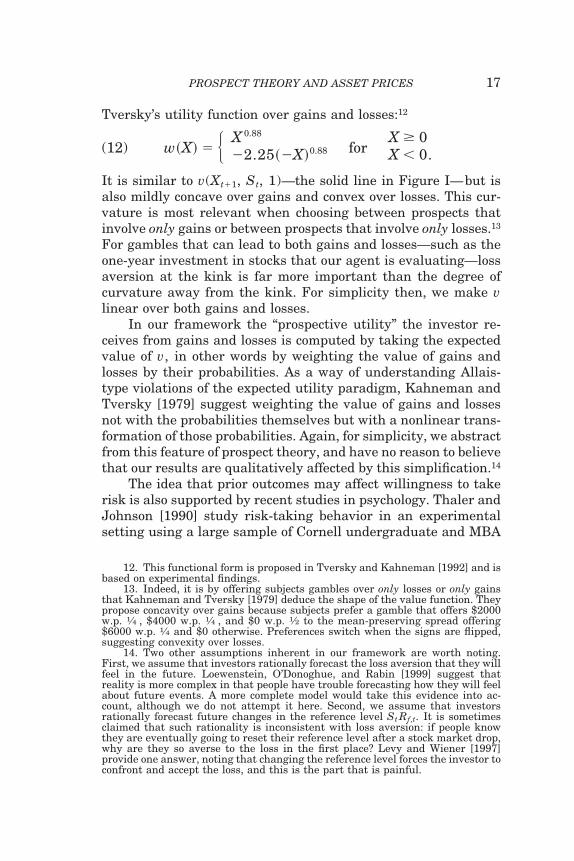
Tversky’s utility function over gains and losses:12

(12) w�X� � � X 0.88

2.25�X�0.88 forX � 0X � 0.

It is similar to v(Xt�1, St, 1)—the solid line in Figure I—but isalso mildly concave over gains and convex over losses. This cur-vature is most relevant when choosing between prospects thatinvolve only gains or between prospects that involve only losses.13

For gambles that can lead to both gains and losses—such as theone-year investment in stocks that our agent is evaluating—lossaversion at the kink is far more important than the degree ofcurvature away from the kink. For simplicity then, we make vlinear over both gains and losses.

In our framework the “prospective utility” the investor re-ceives from gains and losses is computed by taking the expectedvalue of v, in other words by weighting the value of gains andlosses by their probabilities. As a way of understanding Allais-type violations of the expected utility paradigm, Kahneman andTversky [1979] suggest weighting the value of gains and lossesnot with the probabilities themselves but with a nonlinear trans-formation of those probabilities. Again, for simplicity, we abstractfrom this feature of prospect theory, and have no reason to believethat our results are qualitatively affected by this simplification.14

The idea that prior outcomes may affect willingness to takerisk is also supported by recent studies in psychology. Thaler andJohnson [1990] study risk-taking behavior in an experimentalsetting using a large sample of Cornell undergraduate and MBA

12. This functional form is proposed in Tversky and Kahneman [1992] and isbased on experimental findings.

13. Indeed, it is by offering subjects gambles over only losses or only gainsthat Kahneman and Tversky [1979] deduce the shape of the value function. Theypropose concavity over gains because subjects prefer a gamble that offers $2000w.p. 1⁄4 , $4000 w.p. 1⁄4 , and $0 w.p. 1⁄2 to the mean-preserving spread offering$6000 w.p. 1⁄4 and $0 otherwise. Preferences switch when the signs are flipped,suggesting convexity over losses.

14. Two other assumptions inherent in our framework are worth noting.First, we assume that investors rationally forecast the loss aversion that they willfeel in the future. Loewenstein, O’Donoghue, and Rabin [1999] suggest thatreality is more complex in that people have trouble forecasting how they will feelabout future events. A more complete model would take this evidence into ac-count, although we do not attempt it here. Second, we assume that investorsrationally forecast future changes in the reference level St Rf,t. It is sometimesclaimed that such rationality is inconsistent with loss aversion: if people knowthey are eventually going to reset their reference level after a stock market drop,why are they so averse to the loss in the first place? Levy and Wiener [1997]provide one answer, noting that changing the reference level forces the investor toconfront and accept the loss, and this is the part that is painful.


students. They offer subjects a sequence of gambles and find thatoutcomes in earlier gambles affect subsequent behavior: followinga gain, people appear to be more risk seeking than usual, takingon bets they would not normally accept. This result has becomeknown as the “house money” effect, because it is reminiscent ofthe expression “playing with the house money” used to describegamblers’ increased willingness to bet when ahead. Thaler andJohnson argue that these results suggest that losses are lesspainful after prior gains, perhaps because those gains cushion thesubsequent setback.

Thaler and Johnson also find that after a loss, subjects dis-play considerable reluctance to accept risky bets. They interpretthis as showing that losses are more painful than usual followingprior losses.15

The stakes used in Thaler and Johnson [1990] are small—thedollar amounts are typically in double digits. Interestingly, Gert-ner [1993] obtains similar results in a study involving muchlarger stakes. He studies the risk-taking behavior of participantsin the television game show “Card Sharks,” where contestantsplace bets on whether a card to be drawn at random from a deckwill be higher or lower than a card currently showing. He findsthat the amount bet is a strongly increasing function of thecontestant’s winnings up to that point in the show. Once again,this is evidence of more aggressive risk-taking behavior followingsubstantial gains.

The evidence we have presented suggests that in the contextof a sequence of gains and losses, people are less risk aversefollowing prior gains and more risk averse after prior losses. Thismay initially appear puzzling to readers familiar with Kahnemanand Tversky’s original value function, which is concave in theregion of gains and convex in the region of losses. In particular,the convexity over losses is occasionally interpreted to mean that“after a loss, people are risk seeking,” contrary to Thaler andJohnson’s evidence. Hidden in this interpretation, though, is acritical assumption, namely that people integrate or “merge” theoutcomes of successive gambles. Suppose that you have just suf-fered a loss of $1000, and are contemplating a gamble equally

15. It is tempting to explain these results using a utility function where riskaversion decreases with wealth. However, any utility function with sufficientcurvature to produce lower risk aversion after a $20 gain, regardless of initialwealth level, inevitably makes counterfactual predictions about attitudes to large-scale gambles.


likely to win you $200 as to lose you $200. Integration of outcomesmeans that you make the decision about whether to take thegamble by comparing the average of w(1200) and w(800)with w(1000), where w is defined in equation (12). Of course,under this assumption, convexity in the region of losses leads torisk seeking after a loss.

The idea that people integrate the outcomes of sequentialgambles, while appealingly simple, is only a hypothesis. Tverskyand Kahneman [1981] themselves note that prospect theory wasoriginally developed only for elementary, one-shot gambles andthat any application to a dynamic context must await furtherevidence on how people think about sequences of gains and losses.A number of papers, including Thaler and Johnson [1990], havetaken up this challenge, conducting experiments on whether peo-ple integrate sequential outcomes, segregate them, or do some-thing else again. That these experiments have uncovered in-creased risk aversion after prior losses does not contradictprospect theory; it simply rejects the hypothesis that people in-tegrate sequential gambles.16

Thaler and Johnson [1990] do find some situations whereprior losses lead to risk-seeking behavior. These are situationswhere after the prior loss, the subject can take a gamble thatoffers a good chance of breaking even and only limited downside.In conjunction with the other evidence, this suggests that whilelosses after prior losses are very painful, gains that enable peoplewith prior losses to break even are especially sweet. We have notbeen able to introduce this break-even effect into our frameworkin a tractable way. It is worth noting, though, that outside of thespecial situations uncovered by Thaler and Johnson, it is in-creased risk aversion that appears to be the norm after priorlosses.

IV. EQUILIBRIUM PRICES

We now derive equilibrium asset prices in an economy popu-lated by investors with preferences of the type described in Sec-

16. There is another sense in which integration of sequential outcomes is animplausible way to implement prospect theory in a multiperiod context. If inves-tors did integrate many years of stock market gains and losses, they wouldessentially be valuing absolute levels of wealth, and not the changes in wealththat are so important to prospect theory. We thank J. B. Heaton for thisobservation.


tion II. It may be helpful to summarize those preferences here.Each investor chooses consumption Ct and an allocation to therisky asset St to maximize

(13) E� �t�0

� �tCt

1�

1 � �� b0C� t

�t�1v�Xt�1,St,zt�� ,

subject to the standard budget constraint, where

(14) Xt�1 � StRt�1 � StRf,t,

and where for zt � 1,

(15) v�Xt�1,St,zt�



Rt�1 � ztRf,t

Rt�1 � ztRf,t,

and for zt � 1,

(16)

v�Xt�1,St,zt� � � StRt�1 � StRf,t

�� zt��StRt�1 � StRf,t�for

Rt�1 � Rf,t

Rt�1 � Rf,t,

with

(17) �� zt� � � � k� zt � 1�.

Equations (15) and (16) are pictured in Figure I. Finally, thedynamics of the state variable zt are given by

(18) zt�1 � ��zt

R�

Rt�1� � �1 � ��1�.

We calculate the price Pt of a dividend claim—in other words,the stock price—in two different economies. The first economy,which we call “Economy I,” is the one analyzed by Lucas [1978].It equates consumption and dividends so that stocks are modeledas a claim to the future consumption stream.

Due to its simplicity, the first economy is the one typicallystudied in the literature. However, we also calculate stock pricesin a more realistic economy—“Economy II”—where consumptionand dividends are modeled as separate processes. We can thenallow the volatility of consumption growth and of dividend growthto be very different, as they indeed are in the data. We can thinkof the difference between consumption and dividends as arising


from the fact that investors have other sources of income besidesdividends. Equivalently, they have other forms of wealth, such ashuman capital, beyond their financial assets.

In our model, changes in risk aversion are caused by changesin the level of the stock market. In this respect, our approachdiffers from consumption-based habit formation models, wherechanges in risk aversion are due to changes in the level of con-sumption. While these are different ideas, it is not easy to illus-trate their distinct implications in an economy like Economy I,where consumption and the stock market are driven by a singleshock, and are hence perfectly conditionally correlated. This iswhy we emphasize Economy II: since consumption and dividendsdo not have to be equal in equilibrium, we can model them asseparate processes, driven by shocks that are only imperfectlycorrelated. The contrast between our approach and the consump-tion-based framework then becomes much clearer.

In both economies, we construct a one-factor Markov equilib-rium in which the risk-free rate is constant and the Markov statevariable zt determines the distribution of future stock returns.Specifically, we assume that the price-dividend ratio of the stockis a function of the state variable zt:

(19) ft � Pt /Dt � f� zt�,

and then show for each economy in turn that there is indeed anequilibrium satisfying this assumption. Given the one-factor as-sumption, the distribution of stock returns Rt�1 is determined byzt and the function f� using

(20) Rt�1 �Pt�1 � Dt�1

Pt�

1 � Pt�1/Dt�1

Pt /Dt

Dt�1

Dt

�1 � f� zt�1�

f� zt�

Dt�1

Dt.

A. Stock Prices in Economy I

In the first economy we consider, consumption and dividendsare modeled as identical processes. We write the process foraggregate consumption C� t as

(21) log�C� t�1/C� t� � log�Dt�1/Dt� � gC � �C�t�1,

where �t � i.i.d. N(0,1). Note from equation (1) that the mean gD

and volatility �D of dividend growth are constrained to equal gC


and �C, respectively. Together with the one-factor Markov as-sumption, this means that the stock return is given by

(22) Rt�1 �1 � f� zt�1�

f� zt�egC��C�t�1.

Intuitively, the value of the risky asset can change because ofnews about consumption �t�1 or because the price-dividend ratiof changes. Changes in f are driven by changes in zt, which mea-sures past gains and losses: past gains make the investor less riskaverse, raising f, while past losses make him more risk averse,lowering f.

In equilibrium, and under rational expectations about stockreturns and aggregate consumption levels, the agents in oureconomy must find it optimal to consume the dividend stream andto hold the market supply of zero units of the risk-free asset andone unit of stock at all times.17 Proposition 1 characterizes theequilibrium.18

PROPOSITION 1. For the preferences given in (13)–(18), there existsan equilibrium in which the gross risk-free interest rate isconstant at

(23) Rf � 1e�gC�2�C2 / 2,

and the stock’s price-dividend ratio f�, as a function of thestate variable zt, satisfies for all zt:

(24) 1 � Et�1 � f �zt�1�

f �zt�e�1�� gC��C�t�1�� b0Et�v̂�1 � f �zt�1�

f �zt�egC��C�t�1, zt��,

where for zt � 1,

(25) v̂�Rt�1, zt�

� � Rt�1 � Rf,t

�zt Rf,t � Rf,t� � ��Rt�1 � zt Rf,t�for

Rt�1 � zt Rf,t

Rt�1 � zt Rf,t,

17. We need to impose rational expectations about aggregate consumptionbecause the agent’s utility includes aggregate consumption as a scaling term.

18. We assume that log � (1 �) gC � 0.5(1 �)2�C2 0 so that the

equilibrium is well behaved at t � �.


and for zt � 1,

(26) v̂�Rt�1, zt� � � Rt�1 � Rf,t

��zt��Rt�1 � Rf,t�for

Rt�1 � Rf,t

Rt�1 � Rf,t.

We prove this formally in the Appendix. At a less formallevel, our results follow directly from the agent’s Euler equationsfor optimality at equilibrium, derived using standard perturba-tion arguments:

(27) 1 � RfEt��C� t�1/C� t��,

(28) 1 � Et�Rt�1�C� t�1/C� t�� b0Et�v̂�Rt�1, zt��.

Readers may find it helpful to compare these equations withthose derived from standard asset pricing models with powerutility over consumption. The Euler equation for the risk-freerate is the usual one: consuming a little less today and investingthe savings in the risk-free rate does not change the investor’sexposure to losses on the risky asset. The first term in the Eulerequation for the risky asset is also the familiar one first obtainedby Mehra and Prescott [1985]. However, there is now an addi-tional term. Consuming less today and investing the proceeds inthe risky asset exposes the investor to the risk of greater losses.Just how dangerous this is, is determined by the state variable zt.

In constructing the equilibrium in Proposition 1, we followthe assumption laid out in subsection II.D, namely that buying orselling on the part of the investor does not affect the evolution ofthe state variable zt. Equivalently, the investor believes that hisactions will have no impact on the future evolution of zt. As weargued earlier, this is a reasonable assumption for many actionsthe investor might take, but is less so in the case of a completeexit from the stock market. In essence, our assumption meansthat the investor does not consider using his cushion of priorgains in a strategic fashion, perhaps by waiting for the cushion tobecome large, exiting from the stock market so as to preserve thecushion and then reentering after a market crash when expectedreturns are high.19

19. Allowing the investor to consider such strategies does not change thequalitative nature of our results. It may affect our quantitative results dependingon how one specifies the evolution of the investor’s cushion of prior gains after heleaves the stock market.


B. Stock Prices in Economy II

In Economy II, consumption and dividends follow distinctprocesses. This allows us to model the stock for what it really is,namely a claim to the dividend stream, rather than as a claim toconsumption. Formally, we assume

(29) log�C� t�1/C� t� � gC � �C�t�1,

and

(30) log�Dt�1/Dt� � gD � �D�t�1,

where

(31) � �t

�t� � i.i.d. N�� 0

0 � , � 1 �� 1 �� .

This assumption, which makes log C� t/Dt a random walk, allowsus to construct a one-factor Markov equilibrium in which therisk-free interest rate is constant and the price-dividend ratio ofthe stock is a function of the state variable zt.20 The stock returncan then be written as

(32) Rt�1 �1 � f� zt�1�

f� zt�egD��D�t�1.

Given that the consumption and dividend processes are dif-ferent, we need to complete the model specification by assumingthat each agent also receives a stream of nonfinancial income{Yt}—labor income, say. We assume that {Yt} and {Dt} form ajoint Markov process whose distribution gives C� t � Dt � Yt andDt the distributions in (29)–(31).

We construct the equilibrium through the Euler equations ofoptimality (27) and (28). The risk-free rate is again constant andgiven by (27). The one-factor Markov structures of stock prices in(19) and (32) satisfy the Euler equation (28). The next propositioncharacterizes this equilibrium. The Appendix gives more detailedcalculations and proves that the Euler equations indeed charac-terize optimality.21

20. Another approach would model C� t and Dt as cointegrated processes, butwe would then need at least one more factor to characterize equilibrium prices.

21. We assume that log �gC � gD � 0.5(�2�C2 2��C�D � �D

2 ) 0 sothat the equilibrium is well behaved at t � �.


PROPOSITION 2. In Economy II, the risk-free rate is constant at

(33) Rf � 1e�gC�2�C2 / 2,

and the stock’s price-dividend ratio f� is given by

(34) 1 � egD�gC��2�c2�1�2�/ 2Et�1 � f �zt�1�

f �zt�e��D��C��t�1�

� b0Et�v̂�1 � f �zt�1�

f �zt�egD��D�t�1, zt��,

where v̂ is defined in Proposition 1.

C. Model Intuition

In Section V we solve for the price-dividend ratio numericallyand use simulated data to show that our model provides a way ofunderstanding a number of puzzling empirical features of aggre-gate stock returns. In particular, our model is consistent with alow volatility of consumption growth on the one hand, and a highmean and volatility of stock returns on the other, while maintain-ing a low and stable risk-free rate. Moreover, it generates longhorizon predictability in stock returns similar to that observed inempirical studies and predicts a low correlation between con-sumption growth and stock returns.

It may be helpful to outline the intuition behind these resultsbefore moving to the simulations. Return volatility is a good placeto start: how can our model generate returns that are morevolatile than the underlying dividends? Suppose that there is apositive dividend innovation this period. This will generate a highstock return, increasing the investor’s reserve of prior gains. Thismakes him less risk averse, since future losses will be cushionedby the prior gains, which are now larger than before. He thereforediscounts the future dividend stream at a lower rate, giving stockprices an extra jolt upward. A similar story holds for a negativedividend innovation. It generates a low stock return, depletingprior gains or increasing prior losses. The investor is more riskaverse than before, and the increase in risk aversion pushesprices still lower. The effect of all this is to make returns sub-stantially more volatile than dividend growth.

The same mechanism also produces long horizon predictabil-ity. Put simply, since the investor’s risk aversion varies over timedepending on his investment performance, expected returns on


the risky asset also vary. To understand this in more detail,suppose once again that there is a positive shock to dividends.This generates a high stock return, which lowers the investor’srisk aversion and pushes the stock price still higher, leading to ahigher price-dividend ratio. Since the investor is less risk averse,subsequent stock returns will be lower on average. Price-dividendratios are therefore inversely related to future returns, in exactlythe way that has been documented by numerous studies, includ-ing Campbell and Shiller [1988] and Fama and French [1988b].

If changing loss aversion can indeed generate volatile stockprices, then we may also be able to generate a substantial equitypremium. On average, the investor is loss averse, and fears thefrequent drops in the stock market. He may therefore charge ahigh premium in return for holding the risky asset. Earlier re-search provides hope that this will be the case: Benartzi andThaler [1995] analyze one-period portfolio choice for loss-averseinvestors—a partial equilibrium analysis where the stock mar-ket’s high historical mean and volatility are exogenous—and findthat these investors are unwilling to invest much of their wealthin stocks, even in the face of the large historical premium. Thissuggests that loss aversion may be a useful ingredient for equi-librium models trying to understand the equity premium.

Finally, our framework also generates stock returns that areonly weakly correlated with consumption, as in the data.22 Tounderstand this, note that in our model, stock returns are madeup of two components: one due to news about dividends, and theother to a change in risk aversion caused by movements in thestock market. Both components are ultimately driven by shocksto dividends, and so in our model, the correlation between returnsand consumption is very similar to the correlation between divi-dends and consumption—a low number. This result distinguishesour approach from consumption-based habit formation models ofthe stock market such as Campbell and Cochrane [1999]. In thosemodels, changes in risk aversion are caused by changes in con-sumption levels. This makes it inevitable that returns will besignificantly correlated with consumption shocks, in contrast towhat we find in the data.

Another well-known difficulty with consumption-based mod-els is that attempts to make them match features of the stock

22. This is a feature that is unique to Economy II, which allows for ameaningful distinction between consumption and dividends.


market often lead to counterfactual predictions for the risk-freerate. For example, these models typically explain the equitypremium with a high curvature � of utility over consumption.However, this high � also leads to a strong desire to smoothconsumption intertemporally, generating high interest rates.Furthermore, the habit formation feature that many consump-tion-based models use to explain stock market volatility can alsomake interest rates counterfactually volatile.23

In our framework we use loss aversion over financial wealthfluctuations rather than a high curvature of utility over consump-tion to explain the equity premium. We do not therefore generatea counterfactually high interest rate. Moreover, since changes inrisk aversion are driven by past stock market performance ratherthan by consumption, we can maintain a stable, indeed constantinterest rate.

One feature that our model does share with consumption-based models like that of Campbell and Cochrane [1999] is con-trarian expectations on the part of investors. Since stock prices inthese models are high when investors are less risk averse, theseare also times when investor require—and expect—lower returnsthan on average.

Durell [1999] has examined investor expectations about fu-ture stock market behavior and found evidence of extrapolative,rather than contrarian expectations. In other words, some inves-tors appear to expect higher than average returns precisely atmarket peaks. Shiller [1999] presents results of a survey of in-vestor expectations over the course of the U. S. bull market of thelast few years. He finds no evidence of extrapolative expectations;but neither does he find evidence of contrarian expectations. It isnot clear whether the samples used by Durell and Shiller arerepresentative of the investing population, but they do suggestthat the story in this paper—or indeed the consumption-basedstory—may not be a complete description of the facts.

D. A Note on Aggregation

The equilibrium pricing equations in subsections IV.A andIV.B are derived under the assumption that the investors in our

23. Campbell and Cochrane’s paper [1999] is perhaps the only consumption-based model that avoids problems with the risk-free rate. A clever choice offunctional form for the habit level over consumption enables them to use precau-tionary saving to counterbalance the strong desire to smooth consumptionintertemporally.


economy are completely homogeneous. This is certainly a strongassumption. Investors may be heterogeneous along numerousdimensions, which raises the question of whether the intuition ofour model still goes through once investor heterogeneity is recog-nized. For any particular form of heterogeneity, we need to checkthat loss aversion remains in the aggregate and, moreover, thataggregate loss aversion still varies with prior stock market move-ments. If these two elements are still present, our model shouldstill be able to generate a high premium, volatility, andpredictability.

One form of heterogeneity does aggregate satisfactorily: thisis the case where investors have different wealth levels, butidentical wealth to income ratios. We can model this by havingseveral cohorts of investors, each cohort containing a continuumof equally wealthy investors. Since wealth is not a nontrivial statevariable, all our results go through.24

There is reason to hope that our intuition will also surviveother forms of heterogeneity. For example, it is possible thatinvestors differ in the extent of their prior gains or losses, perhapsbecause they entered the stock market at different times. In otherwords, investors may have different zt’s.

Note that even if zt varies across investors, each individualinvestor is still more sensitive to losses than to gains, and thereis no reason to believe that this will be lost in the aggregate.Hence there is no reason to think that the equity premium will bemuch reduced in the presence of this kind of heterogeneity. Fur-thermore, if the stock market experiences a sustained rise, thiswill increase prior gains for most investors, making them less riskaverse. Therefore, it is very reasonable to think that risk aversionwill also fall in the aggregate. If aggregate loss aversion stillvaries over time, our model should still be able to generate sub-stantial volatility and predictability.

V. NUMERICAL RESULTS AND FURTHER DISCUSSION

In this section we present price-dividend ratios f( zt) thatsolve equations (24) and (34). We then create a long time series ofsimulated data and use it to compute various moments of asset

24. The only subtlety is that since aggregate consumption C� t enters prefer-ences, we need to assume that people use the average consumption of a referencegroup of people with identical wealth to set C� t, rather than average consumptionin the economy as a whole.


returns which can be compared with historical numbers. We dothis for both economies described in Section IV: Economy I, wherestocks are modeled as a claim to the consumption stream; and themore realistic Economy II where stocks are a claim to dividends,which are no longer the same as consumption.

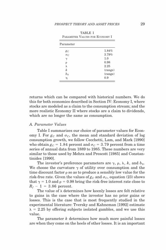
A. Parameter Values

Table I summarizes our choice of parameter values for Econ-omy I. For gC and �C, the mean and standard deviation of logconsumption growth, we follow Cecchetti, Lam, and Mark [1990]who obtain gC � 1.84 percent and �C � 3.79 percent from a timeseries of annual data from 1889 to 1985. These numbers are verysimilar to those used by Mehra and Prescott [1985] and Constan-tinides [1990].

The investor’s preference parameters are �, , �, k, and b0.We choose the curvature � of utility over consumption and thetime discount factor so as to produce a sensibly low value for therisk-free rate. Given the values of gC and �C, equation (23) showsthat � � 1.0 and � 0.98 bring the risk-free interest rate close toRf 1 � 3.86 percent.

The value of � determines how keenly losses are felt relativeto gains in the case where the investor has no prior gains orlosses. This is the case that is most frequently studied in theexperimental literature: Tversky and Kahneman [1992] estimate� � 2.25 by offering subjects isolated gambles, and we use thisvalue.

The parameter k determines how much more painful lossesare when they come on the heels of other losses. It is an important

TABLE IPARAMETER VALUES FOR ECONOMY I

Parameter

gC 1.84%�C 3.79%� 1.0 0.98� 2.25k (range)b0 (range)� 0.9


determinant of the investor’s average degree of loss aversion overtime. In the results that we present, we pick k in two differentways. Our first approach is to choose k so as to make the inves-tor’s average loss aversion close to 2.25, where average loss aver-sion is computed in a way that we make precise in the Appendix.After prior gains, the investor does not fear losses very much, sohis effective loss aversion is less than 2.25; after prior losses, heis all the more sensitive to additional losses, so his effective lossaversion is higher than 2.25, to a degree governed by k. We findthat choosing k � 3 keeps average loss aversion close to 2.25. Tounderstand what a k of 3 means, suppose that the state variablezt is initially equal to 1, and that the stock market then experi-ences a sharp fall of 10 percent. From equation (10) with � � 1,this means that zt increases by approximately 0.1, to 1.1. From(8), any additional losses will now penalized at 2.25 � 3(0.1) �2.55, a slightly more severe penalty.

Our second approach to picking k is to go to the data forguidance: we simply look for values of k that bring the predictedequity premium close to its empirical value.

The parameter b0 determines the relative importance of theprospect utility term in the investor’s preferences. We do not havestrong priors about what constitutes a reasonable value for b0 andso present results for a range of values.25

The two final parameters, � and R� , arise in the definition ofthe state variable dynamics. R� is not a parameter we have anycontrol over: it is completely determined by the other parametersand the requirement that the equilibrium median value of zt beequal to one. The variable � controls the persistence of zt andhence also the persistence of the price-dividend ratio. We findthat an � of 0.9 brings the autocorrelation of the price-dividendratio that we generate close to its empirical value.

B. Methodology

Before presenting our results, we briefly describe the waythey were obtained. The identical technique is used for bothEconomy I and II, so we describe it only for the case of EconomyI. The difficulty in solving equation (24) comes from the fact that

25. One way to think about b0 is to compare the disutility of losing a dollar inthe stock market with the disutility of having to consume a dollar less. Whencomputed at equilibrium, the ratio of these two quantities equals b0�. By plug-ging numbers into this expression, we can see how b0 controls the relativeimportance of consumption utility and nonconsumption utility.


zt�1 is a function of both �t�1 and f�. In economic terms, our statevariable is endogenous: it tracks prior gains and losses, whichdepend on past returns, themselves endogenous. Equation (24) istherefore self-referential and needs to be solved in conjunctionwith

(35) zt�1 � ��zt

R�

Rt�1� � �1 � ��1�,

and

(36) Rt�1 �1 � f� zt�1�

f� zt�egC��C�t�1.

We use the following technique. We start out by guessing asolution to (24), f (0) say. We then construct a function h(0) so thatzt�1 � h(0)( zt, �t�1) solves equations (35) and (36) for this f � f (0).The function h(0) determines the distribution of zt�1 conditionalon zt.

Given the function h(0), we get a new candidate solution f (1)

through the following recursion:

(37) 1 � Et�1 � f �i�� zt�1�

f �i�1�� zt�e�1�� gC��C�t�1��

� b0Et� v̂�1 � f �i�� zt�1�

f �i�1�� zt�egC��C�t�1, zt�� , � zt.

With f (1) in hand, we can calculate a new h � h(1) that solvesequations (35) and (36) for f � f (1). This h(1) gives us a newcandidate f � f (2) from (37). We continue this process untilconvergence occurs: f (i) 3 f, and h(i) 3 h.

C. Stock Prices in Economy I

Figure III presents price-dividend ratios f( zt) that solveequation (24) for three different values of b0: 0.7, 2, and 100, andwith k fixed at 3. Note that f( zt) is a decreasing function of zt inall cases. The intuition for this is straightforward: a low value ofzt means that recent returns on the asset have been high, givingthe investor a reserve of prior gains. These gains cushion subse-quent losses, making the investor less risk averse. He thereforediscounts future dividends at a lower rate, raising the price-dividend ratio. Conversely, a high value of zt means that the


investor has recently experienced a spate of painful losses; he isnow especially sensitive to further losses which makes him morerisk averse and leads to lower price-dividend ratios.

Figure III by itself does not tell us the range of price-dividendratios we are likely to see in equilibrium. For that, we need toknow the equilibrium distribution of the state variable zt. FigureIV shows this distribution for one case that we will consider inmore detail later: b0 � 2, k � 3. To obtain it, we draw a long timeseries {�t}t�1

50,000 of 50,000 independent draws from the standardnormal distribution and starting with z0 � 1, use the functionzt�1 � h( zt, �t�1) described in subsection V.B to generate a timeseries for zt. Note from the graph that the average zt is close toone, and this is no accident. The value of R� in equation (10) ischosen precisely to make the median value of zt as close to one aspossible.

FIGURE IIIPrice-Dividend Ratios in Economy I

The price-dividend ratios are plotted against zt, which measures prior gains andlosses: a low zt indicates prior gains. The parameter b0 controls how much theinvestor cares about financial wealth fluctuations. We fix the parameter k at 3,bringing average loss aversion close to 2.25 in all cases.


As we generate the time series for zt period by period, we alsocompute the returns along the way using equation (20). We nowpresent sample moments computed from these simulated re-turns. The time series is long enough that sample momentsshould serve as good approximations to population moments.

Table II presents the important moments of stock returns fordifferent values of b0 and k. In the top panel, we vary b0 and setk to 3, which keeps average loss aversion over time close to 2.25.At one extreme we have b0 � 0, the classic case considered byMehra and Prescott [1985]. As we push b0 up, the asset returnmoments eventually reach a limit that is well approximated witha b0 of 100. The table also reports the investor’s average lossaversion, calculated in the way described in the Appendix.

Note that as we raise b0 while keeping k fixed, the equitypremium goes up. There are two forces at work here. As b0 getslarger, prior outcomes affect the investor more, causing his risk

FIGURE IVDistribution of the State Variable zt

The distribution is based on Economy I with b0 � 2 and k � 3.


aversion to vary more, and hence generating more volatile stockreturns. Moreover, as b0 grows, loss aversion becomes a moreimportant feature of the investor’s preferences, pushing up theSharpe ratio. The higher volatility and higher Sharpe ratio com-bine to raise the equity premium.

Although the results in Table II are encouraging from aqualitative standpoint, the magnitudes are not impressive.Changes in risk aversion do give returns a volatility higher thanthe 3.79 percent volatility assumed for dividend growth, but thiseffect is not nearly large enough to match historical volatility.Since the investor does not observe any particularly large marketcrashes, he does not charge a particularly high equity premiumeither. The highest equity premium we can possibly generate forthis value of k is 1.28 percent.

The bottom panel of Table II shows that we can come closerto matching the historical equity premium by increasing thevalue of k. Since the investor is now extremely loss averse in somestates of the world, average loss aversion also climbs steeply.Note, however, that return volatility here is still far too low.

TABLE IIASSET RETURNS IN ECONOMY I

b0 � 0 b0 � 0.7 b0 � 2 b0 � 100 Empiricalvaluek � 3 k � 3 k � 3

Log risk-free rate 3.79 3.79 3.79 3.79 0.58Log excess stock return

Mean 0.07 0.63 0.88 1.26 6.03Standard deviation 3.79 4.77 5.17 5.62 20.02Sharpe ratio 0.02 0.13 0.17 0.22 0.3

Average loss aversion 2.25 2.25 2.25

b0 � 0.7 b0 � 2 b0 � 100k � 150 k � 100 k � 50

Log risk-free rate 3.79 3.79 3.79Log excess stock return

Mean 3.50 3.66 3.28Standard deviation 10.43 10.22 9.35Sharpe ratio 0.34 0.36 0.35


Moments of asset returns are expressed as annual percentages. Empirical values are based on TreasuryBill and NYSE data from 1926–1995. The parameter b0 controls how much the investor cares about financialwealth fluctuations, while k controls the increase in loss aversion after a prior loss.


An unrealistic feature of Economy I is that consumption anddividends are constrained to follow the same process. This meansthat we are modeling stocks as a claim to a very smooth consump-tion stream, rather than as what they really are, namely a claimto a far more volatile dividend stream. We therefore turn toEconomy II which allows us to relax this constraint.

D. Stock Prices in Economy II

We now calculate stock prices in a more general economywhere consumption and dividends are modeled as distinct pro-cesses. Table III presents our choice of parameters in this econ-omy. To make comparison easier, we also show the parametersused for Economy I alongside.

Allowing consumption and dividends to follow different pro-cesses introduces three new parameters: gD, the mean dividendgrowth rate; �D, the volatility of dividend growth; and �, thecorrelation of shocks to dividend growth and consumptiongrowth. For simplicity, we set gD � gC � 0.0184. Using NYSEdata from 1926–1995 from CRSP, we find �D � 0.12. Campbell[2000] estimates � in a time series of U. S. data spanning the pastcentury, and based on his results, we set � � 0.15. As the tableshows, we keep all other parameters fixed at the values discussedin subsection V.A.

Figure V presents price-dividend ratios that solve equation

TABLE IIIPARAMETER VALUES FOR ECONOMY II

Parameter Economy II Economy I

gC 1.84% 1.84%gD 1.84% —�C 3.79% 3.79%�D 12.0% —� 0.15 —� 1.0 1.0 0.98 0.98� 2.25 2.25k (range) (range)b0 (range) (range)� 0.9 0.9

The parameter values used for Economy I and shown inTable I are repeated here for ease of comparison.


(34) for three different values of b0: 0.7, 2, and 100, with k fixedat 3. Unconditional moments of stock returns are shown in TableIV for various values of b0 and k. The top panel keeps k fixed at3, bringing the average degree of loss aversion close to 2.25. Aquick comparison with Table II shows that separating consump-tion and dividends improves the results significantly. The vola-tility of returns is now much higher than what we obtained inEconomy I because dividend growth volatility is now 12 percentrather than just 3.79 percent. The equity premium is also muchhigher: the investor now sees far more severe downturns in thestock market and charges a much larger premium ascompensation.

Modeling consumption and dividends separately also leads tohigher return volatility in consumption-based models such asthat of Campbell and Cochrane [1999]. However, the fact that the

FIGURE VPrice-Dividend Ratios in Economy II

The price-dividend ratios are plotted against zt, which measures prior gains andlosses: a low zt indicates prior gains. The parameter b0 controls how much theinvestor cares about financial wealth fluctuations. We fix the parameter k at 3,bringing average loss aversion close to 2.25 in all cases.


equity premium goes up is unique to our model: as Campbell andCochrane demonstrate, separating consumption and dividendshas no effect on the equity premium in a consumption-basedmodel. The reason is that in a consumption-based model, thecanonical measure of a stock’s risk is its covariance with con-sumption growth. By separating consumption and dividends, thevolatility of stock returns goes up, but the correlation of stockreturns with consumption goes down, since dividends are poorlycorrelated with consumption. Overall, the covariance with con-sumption remains unaffected, and the equity premium remainsas hard to explain as before.

TABLE IVASSET PRICES AND RETURNS IN ECONOMY II

b0 � 0 b0 � 0.7 b0 � 2 b0 � 100 Empiricalk � 3 k � 3 k � 3 value


Mean 0.65 1.3 2.62 3.68 6.03Standard deviation 12.0 17.39 20.87 20.47 20.02Sharpe ratio 0.05 0.07 0.13 0.18 0.3Correlation w/consumption

growth 0.15 0.15 0.15 0.15 0.1Price-dividend ratio

Mean 76.6 29.8 22.1 17.5 25.5Standard deviation 0 2.9 2.7 2.4 7.1


b0 � 0.7 b0 � 2 b0 � 100k � 20 k � 10 k � 8

Log risk-free rate 3.79 3.79 3.79Log excess stock return

Mean 5.17 5.02 5.88Standard deviation 25.85 23.84 24.04Sharpe ratio 0.2 0.21 0.24Correlation w/consumptiongrowth 0.15 0.15 0.15

Price-dividend ratioMean 14.0 14.6 12.7Standard deviation 2.6 2.5 2.2


Moments of asset returns are expressed as annual percentages. Empirical values are based on TreasuryBill and NYSE data from 1926–1995. The parameter b0 controls how much the investor cares about financialwealth fluctuations, while k controls the increase in loss aversion after a prior loss.


The investor in our model cares not only about consumptionbut also about fluctuations in the value of his investments. Anincrease in dividend volatility makes stocks more volatile, scaringthe investor into charging a higher equity premium. It is true thatstocks are now less correlated with consumption, but this does notmatter in our model, since the investor cares about fluctuations inthe stock market per se, not merely about how those fluctuationscovary with consumption growth.

Table IV confirms that stock returns are only weakly corre-lated with consumption growth in our model. As discussed ear-lier, this prediction is unique to our framework: since consump-tion-based models ascribe a significant fraction of price volatilityto changes in consumption, stock returns are inevitably highlycorrelated with consumption growth.

We also report the mean and standard deviation of thesimulated price-dividend ratio. It is striking that while we aresuccessful at matching the volatility of returns, we significantlyunderpredict the volatility of the price-dividend ratio. To under-stand how this can be, it is helpful to consider the followingapproximate relationship, derived by Campbell, Lo, and MacKin-lay [1997] with the help of a log-linear approximation26:

rt�1 A � log ft�1 � log ft � �D�t�1.

In words, up to a constant A, the log return rt�1 is approximatelyequal to the change in the log price-dividend ratio plus the inno-vation to dividend growth �D�t�1. This gives

var�rt�1� var� logft�1

ft� � �D

2 � 2 cov� logft�1

ft, �D�t�1� .

Our simulated price-dividend ratio is not sufficiently volatile,making var(log( ft�1/ft) too low in our model relative to what it isin the data. The reason we are still able to match the volatility ofreturns var(rt�1) is that cov(log( ft�1/ft), �D�t�1) is too high in ourmodel relative to what it is in the data: in our framework, changesin price-dividend ratios are perfectly conditionally correlatedwith dividend shocks.

Since our model relies on only one factor to generate move-ment in the price-dividend ratio, it is not surprising that we

26. More specifically, this follows from equation 7.1.19 in Chapter 7 of thebook.


underpredict its volatility. In a more realistic model, other factorswill also affect the price-dividend ratio: consumption relative tohabit is one possible factor suggested by the habit formationliterature. Adding such factors will increase the volatility of theprice-dividend ratio and decrease its correlation with dividendshocks, improving the model’s fit with the data. It is worth em-phasizing, though, that a purely consumption-based approachwill not fare well, since it will predict that changes in price-dividend ratios are perfectly conditionally correlated with con-sumption shocks, and that returns are highly correlated withconsumption. A model that merges habit formation over con-sumption with a direct concern about financial wealth fluctua-tions may be much more fruitful.

The bottom panel in Table IV shows that we can significantlyimprove our results by increasing k, which increases investors’loss aversion after prior losses. In Economy I, we had to make theinvestor extraordinarily loss averse in some states of the world toeven come close to matching the equity premium. Interestingly,the increases in k we need now are much more modest. For b0 �2, for example, a k of 10 is enough to give a premium of 5.02percent and a volatility of 23.84 percent; note also that thiscorresponds to an average loss aversion of only 3.5; this is not asmall level of risk aversion, but neither is it extreme.

Figure VI presents some additional results of interest. Theleft panel plots the conditional expected stock return as a function

FIGURE VIConditional Moments of Stock Returns

The conditional stock return mean and volatility are plotted against zt, whichmeasures prior gains and losses: a low zt indicates prior gains. The results are forEconomy II with b0 � 2 and k � 3. The dashed line in the left-hand panelindicates the level of the risk-free rate.


of zt, obtained by numerically integrating the return equation(32) over the conditional distribution of zt�1 given by zt�1 �h( zt,�t�1). The value of b0 here is 2 and k is 3. The conditionalexpected return is an increasing function of the state variable.Low values of zt mean that the investor has accumulated priorgains that will cushion future losses. He is therefore less riskaverse, leading to a lower expected return in equilibrium. Thedashed line shows the level of the constant risk-free rate forcomparison.

The right panel in Figure VI graphs the conditional volatilityof returns as a function of the state variable. Since much of thereturn volatility in our model is generated by changing riskaversion, the conditional volatility in any state depends on howsensitive the investor’s risk aversion in that state is to dividendshocks. Empirically, volatility has been found to be higher aftermarket crashes than booms, which in our context would mean anupward sloping conditional volatility curve. For much of therange of the state variable, this is exactly what we find. However,this result is sensitive to how we make the degree of loss aversiondepend on prior outcomes, so we do not attach too much weightto it.

Table V presents autocorrelations of log returns and of theprice-dividend ratio. As expected, our model produces negativelyautocorrelated returns at all lags: high prices lower risk aversion

TABLE VAUTOCORRELATIONS OF LOG RETURNS AND PRICE-DIVIDEND RATIOS IN ECONOMY II

b0 � 2 b0 � 2 Empiricalvaluek � 3 k � 10

corr(rt, rtj)j � 1 0.07 0.12 0.07j � 2 0.05 0.09 0.17j � 3 0.04 0.06 0.05j � 4 0.04 0.04 0.11j � 5 0.02 0.03 0.04

corr((P/D)t, (P/D)tj)j � 1 0.81 0.72 0.70j � 2 0.66 0.52 0.50j � 3 0.53 0.38 0.45j � 4 0.43 0.28 0.43j � 5 0.35 0.20 0.40

Empirical values are based on NYSE data from 1926–1995.


and lead to lower returns on average. These negative autocorre-lations imply long horizon mean reversion of the kind docu-mented by Poterba and Summers [1988] and Fama and French[1988a]. Moreover, the price-dividend ratio is highly autocorre-lated in our model, closely matching its actual behavior.

Since the investor’s risk aversion changes over time, ex-pected returns also vary, and hence returns are predictable. Todemonstrate this, we use our simulated data to run regressions ofcumulative log returns over a j-year horizon on the lagged divi-dend-price ratio for j � 1, 2, 3, and 4:

(38) rt�1 � rt�2 � . . . � rt�j � �j � �j�Dt /Pt� � �j,t.

where rt is the log return. Table VI presents the slope coefficients�j and R2( j) obtained from our simulated data alongside theempirical values. Note that our simulated results capture themain features of the empirical findings, including an R2 thatincreases with the return horizon.

E. Sensitivity Analysis

We now analyze the sensitivity of our results to variousparameters of interest. For each parameter that we vary, theother parameters are kept fixed at the values given in Table III.

Table VII shows the effect of varying k, which governs howmuch loss aversion goes up after prior losses. Raising k has alarge effect on the equity premium since it raises average loss

TABLE VIRETURN PREDICTABILITY REGRESSIONS IN ECONOMY II

�j, R2( j)b0 � 2 b0 � 2 Empirical

valuek � 3 k � 10

�1 4.6 4.4 4.2�2 8.3 7.5 8.7�3 11.6 9.7 12.1�4 13.7 11.5 15.9R2(1) 2% 6% 7%R2(2) 4% 10% 16%R2(3) 5% 12% 22%R2(4) 6% 14% 30%

Coefficients and R2 in regressions of j-year cumulative log returns on the lagged dividend-price ratio,rt�1 � rt�2 � . . . � rt�j � �j � �j(Dt /Pt) � �j,t. Empirical values are based on annual NYSE data from1926–1995.


aversion. It also raises volatility somewhat because a higher kmeans more rapid changes in risk aversion.

Throughout our analysis we have fixed � at 2.25 since manyindependent experimental studies have estimated it at aroundthis level. Table VIII shows how the results change as we vary �.An increase in � raises the equity premium because average lossaversion is now higher.

Table IX examines the effect of varying �. This parameterdetermines how far into the future the investor will be affected bya substantial gain or loss this year. The primary effect of � is onvolatility: if � is high, a loss this year will make the investor moreloss averse for many years to come, leading him to discount cashflows at a higher rate many years into the future, and causing amore dramatic price drop today. More directly, � affects the

TABLE VIISENSITIVITY OF ASSET RETURNS TO k

k � 3 k � 5 k � 10Empiricalvalue

Log excess stock returnMean 2.62 3.15 5.02 6.03Standard deviation 20.87 20.93 23.84 20.02Sharpe ratio 0.13 0.15 0.21 0.3


The parameter k controls how much loss aversion increases after a prior loss. Moments of asset returnsare expressed as annual percentages. The results are for Economy II with b0 � 2; other parameters are fixedat the values in Table III.

TABLE VIIISENSITIVITY OF ASSET RETURNS TO �

� � 1.5 � � 2.25 � � 3Empiricalvalue



The parameter � controls the investor’s loss aversion. Moments of asset returns are expressed as annualpercentages. The results are for Economy II with b0 � 2 and k � 10; other parameters are fixed at the valuesin Table III.


persistence of the state variable and hence the autocorrelation ofthe price-dividend ratio.

So far in our analysis, we have taken the length of the periodover which the investor evaluates gains and losses to be one year.Table X analyzes the effect of changing this. It shows that thelength of the evaluation period mainly affects the equity pre-mium: if the investor evaluates more frequently, he is more likelyto experience losses, and since he is averse to losses, he willcharge a higher premium.

As described in Section II, we suppose that the investor usesthe risk-free rate as a reference level when calculating gains andlosses. Table XI studies the sensitivity of our results to that

TABLE IXSENSITIVITY OF ASSET RETURNS TO �

� � 1 � � 0.9 � � 0.8Empiricalvalue

Log excess stock returnMean 7.68 5.02 3.91 6.03Standard deviation 34.54 23.84 19.12 20.02Sharpe ratio 0.22 0.21 0.2 0.3Autocorrelation of price-

dividend ratio 0.81 0.72 0.65 0.7Average loss aversion 4.5 3.5 3.0

The parameter � governs how long-lasting the effects of prior gains and losses are. Moments of assetreturns are expressed as annual percentages. The results are for Economy II with b0 � 2 and k � 10; otherparameters are fixed at the values in Table III.

TABLE XSENSITIVITY OF ASSET RETURNS TO THE EVALUATION PERIOD

6 months 1 year 2 yearsEmpiricalvalue



The evaluation period is the length of time over which the investor measures his gains and losses.Moments of asset returns are expressed as annual percentages. The results are for Economy II with b0 � 2and k � 10; other parameters are fixed at the values in Table III.


assumption. Given the parameter values in Table III, the risk-free rate is Rf 1 � 3.86 percent. The table shows the effect ofusing a reference level that is one or two percentage points lowerthan this. Note that the equity premium falls as we use a lowerreference level: a lower reference point means that the investor isless likely to code stock market movements as losses, and henceless inclined to charge a high premium for holding stocks.

VI. THE IMPORTANCE OF PRIOR OUTCOMES

The model in Section II makes use of both loss aversion andthe effect of prior outcomes to match asset prices. The reader maywonder whether both these ingredients are truly necessary. Afterall, Benartzi and Thaler [1995] show that a loss-averse investor isvery reluctant to allocate much of his portfolio to stocks evenwhen faced with the large historical equity premium. This sug-gests that perhaps an equilibrium model with loss aversion alonewould be enough to understand the data. Is it really necessary toincorporate the effect of prior outcomes?

We answer this by examining the predictions of a version ofthe model of Section II which ignores the effect of prior outcomes.In particular, we make the utility v of a gain or loss a function ofthe gain or loss Xt�1 alone, and remove the dependence on thestate variable zt. In this model, the degree of loss aversion is thesame in all circumstances, regardless of the investor’s prior in-vestment performance.

More formally, the investor chooses consumption Ct and anallocation to the risky asset St to maximize

TABLE XISENSITIVITY OF ASSET RETURNS TO THE REFERENCE LEVEL

0% 1% 2%Empiricalvalue



A “0%” reference level means that the investor compares the stock return with the risk-free rate whenmeasuring gains and losses. “1%” means a reference level one percent lower than the risk-free rate.Moments of asset returns are expressed as annual percentages. The results are for Economy II with b0 � 2and k � 10; other parameters are fixed at the values in Table III.


(39) E� �t�0

� �tCt

1�

1 � �� bt

t�1v�Xt�1�� ,

subject to the standard budget constraint, where

(40) Xt�1 � StRt�1 � StRf,t,

and

(41) v�Xt�1� � � Xt�1

�Xt�1for

Xt�1 � 0Xt�1 � 0.

The next proposition presents the equations that governequilibrium prices in an economy like Economy II where con-sumption and dividends are separated out. We show that there isan equilibrium in which the risk-free rate and the stock’s price-dividend ratio are both constant and stock returns are i.i.d.

PROPOSITION 3. For the preferences given by (39)–(41), there existsan equilibrium in which the gross risk-free interest rate isconstant at(42) Rf � 1e�gC�2�C

2 / 2,

and the stock’s price-dividend ratio, ft, is constant at f andgiven by

(43) 1 � egD�gC��2�c2�1�2�/ 2

1 � ff Et�e��D��C��t�1�

� b0Et�v̂�1 � ff egD��D�t�1��,

where

(44) v̂�Rt�1� � � Rt�1 � Rf,t

��Rt�1 � Rf,t�for

Rt�1 � Rf,t

Rt�1 � Rf,t.

That returns are i.i.d. is a direct consequence of the fact thatthe price-dividend ratio is constant. To see this, note that thestock return is related to the stock’s price-dividend ratio, denotedby ft � Pt/Dt, as follows:

(45) Rt�1 �Pt�1 � Dt�1

Pt�

1 � Pt�1/Dt�1

Pt /Dt

Dt�1

Dt

�1 � ft�1

ft

Dt�1

Dt.


Given the assumption that the dividend growth is i.i.d. (see (1)),a constant price-dividend ratio ft � f implies that stock returnsare i.i.d.

Table XII summarizes our choices of parameter values. Manyof the parameters of the earlier model now no longer play a role.The parameters that remain are gC, gD, �C, �D, �, , �, and b0,and we assign them exactly the same values as those chosenearlier. For comparison, we list the earlier parameters alongside.

Figure VII presents the implied values of the price-dividendratio and equity premium for different values of b0 and Table XIII

TABLE XIIPARAMETER VALUES FOR A MODEL WHERE PRIOR OUTCOMES HAVE NO EFFECT

Parameter Section VI Subsection V.D

gC 1.84% 1.84%gD 1.84% 1.84%�C 3.79% 3.79%�D 12.0% 12.0%� 1.0 1.0 0.98 0.98� 2.25 2.25k — (range)b0 (range) (range)� — 0.9

Parameter values used for Economy II in subsection V.D are presented alongside for comparison.

FIGURE VIIStock Prices and Returns When Prior Outcomes Have No Effect

The price-dividend ratio and the equity premium are plotted against b0, whichcontrols how much the investor cares about financial wealth fluctuations.


reports unconditional moments of returns. By comparing theresults in Table XIII with those in the bottom panel of Table IV,we can isolate the impact of prior outcomes.

Our results suggest that a model which relies on loss aver-sion alone cannot provide a complete description of aggregatestock market behavior. The fundamental weakness of such amodel comes in explaining volatility: the standard deviations ofreturns in Table XIII are much lower than both the empiricalvalue and the values in Table IV. The reason for this failure isstraightforward. Since

(46) Rt�1 �Pt�1 � Dt�1

Pt�

1 � ft�1

ft

Dt�1

Dt�

1 � ff egD��D�t�1,

the volatility of log returns in this model is equal to the volatilityof log dividend growth, namely 12 percent. This problem is notunique to the model of this section, but is shared by all consump-tion-based models with constant discount rates.27

The unrealistically low stock return volatility generated bythe model also hampers its ability to explain the equity premium:the average stock returns in Table XIII are considerably lowerthan the empirical value. Intuitively, even though our investor isloss averse, the stock market fluctuations are not large enough toscare him into demanding a high equity premium as compensa-tion. More generally, our results show that loss aversion can behelpful in understanding the equity premium, but only in con-

27. This category includes papers that use first-order risk-aversion, such asEpstein and Zin [1990]. See Campbell [2000] for a discussion of this issue.

TABLE XIIIASSET RETURNS WHEN PRIOR OUTCOMES HAVE NO EFFECT

b0 � 0 b0 � 0.7 b0 � 2 b0 � 100Empiricalvalue


Mean 0.65 1.30 2.17 2.88 6.03Standard deviation 12.0 12.0 12.0 12.0 20.02Sharpe ratio 0.05 0.11 0.18 0.24 0.3

Moments of asset returns are expressed as annual percentages. Empirical values are based on TreasuryBill and NYSE data from 1926–1995. The parameter b0 controls how much the investor cares about financialwealth fluctuations.


junction with a mechanism that makes stock returns more vola-tile than underlying cash flows. In our model, this mechanism isa changing degree of loss aversion, but it could also be based onchanging perceptions of risk, or excessive extrapolation of cashflows into the future.

VII. CONCLUSION

In this paper we study asset prices in an economy whereinvestors derive direct utility not only from consumption but alsofrom fluctuations in the value of their financial wealth. They areloss averse over these fluctuations and how loss averse they are,depends on their prior investment performance.

Our main finding is that in such an economy, asset pricesexhibit phenomena very similar to what has been observed inhistorical data. In particular, stock returns have a high mean, areexcessively volatile, and are significantly predictable in the timeseries. They are also only weakly correlated with consumptiongrowth.

The analysis in this paper raises a number of questions forfurther investigation. For the sake of simplicity, we have studiedan economy containing a single risky asset. In a more realisticeconomy with many risky assets, it is not immediately clear whatinvestors are loss averse about: do they feel loss averse overchanges in the value of individual securities that they own, oronly over portfolio fluctuations? In essence, this is a questionabout how people summarize and think about their investmentperformance, or about how they do their “mental accounting,” inthe language of psychology. How mental accounting affects assetprices is as yet an unexplored topic.

Another question that may warrant further study asks towhat extent our preferences can explain not only financial databut also experimental evidence on attitudes to risky gambles. Inorder to explain the high equity premium, consumption-basedmodels typically assume a high curvature of utility over consump-tion. As is well-known, this high curvature is consistent withattitudes to small-scale gambles, but unfortunately also predictsthat people will reject extremely attractive large-scale gambles.28

In our model, we do not use a high curvature of utility of con-

28. See, for example, Epstein and Zin [1990] and Kandel and Stambaugh[1991].


sumption, and the loss aversion we assume is not far from thatestimated from experimental evidence. This offers the intriguingpossibility that preferences of the kind studied here may be ableto reconcile attitudes to both large- and small-scale gambles withthe empirical facts about stock returns.

APPENDIX

Proof of Proposition 1. Proposition 1 is a special case ofProposition 2 with Yt � 0 and Ct � Dt for all t.

Proof of Proposition 2. We first show that if the risk-freeinterest rate is given by (33) and stock returns are determined by(18), (19), (32), and (34), then the strategy of consuming Ct � C� t �Dt � Yt and holding the market supply of financial securitiesindeed satisfies the Euler equations of optimality (27) and (28).We then show that these Euler equations are necessary andsufficient conditions for optimality.

Given (29), the interest rate Rf in (33) satisfies the Eulerequation (27). For Euler equation (28), note that zt�1 is deter-mined only by zt and �t�1 through (18) and (32), so we have

Et�Rt�1�C� t�1

C� t�� Et�1 � f� zt�1�

f� zt�egD��D�t�1e�� gC��C�t�1��

� egD�gCEt�Et�e��C�t�1�t�1�e�D�t�11 � f� zt�1�

f� zt��

� egD � �gC � �2�c2�1 � �2�/ 2Et�1 � f� zt � 1�

f� zt�e��D � ��C��t�1� .

Applying this, we find that the strategy of consuming C� t andholding the market securities indeed satisfies Euler equation(28).

Euler equations are necessary conditions for optimality. Toprove that they are sufficient conditions as well, we apply amethod used by Duffie and Skiadas [1994] and Constantinidesand Duffie [1996].

To simplify notation, let ut(Ct) � tCt1�/(1 �) and b� t �

t�1bt. Assume that the strategy (C*,S*) satisfies the Eulerequations,

(47) u�t�C*t� � RfEt�u�t�1�C*t�1��,


(48) u�t�C*t� � Et�Rt�1u�t�1�C*t�1�� b� tEt�v̂�Rt�1, zt��.

Consider any alternative strategy (C* � �C, S* � �S) thatsatisfies the budget constraint

(49) �Wt�1 � ��Wt � �Ct� Rf � �St�Rt�1 � Rf�.

The increase in expected utility from using the alternative strat-egy is

(50) E� �t�0

�

�ut�C*t � �Ct� � ut�C*� � b� t�Stv̂�Rt�1,zt��(51) � ��C,�S� � E� �

t�0

�

�u�t�C*t��Ct � b� t�Stv̂�Rt�1,zt�� ,

where we have made use of the concavity of ut� and the linearityof the prospect utility term with respect to St. It is thereforeenough to show that �(�C,�S) � 0 under budget constraint (49).

Multiplying u�t�1(C*t�1) with (49) and applying Euler equa-tions (47) and (48), we have

(52) Et�u�t�C*t��Ct � b� t�Stv̂�Rt�1, zt��

� u�t�C*t��Wt � Et�u�t�1�C*t�1��Wt�1�.

Summing up (52) for all t and taking expectations, we have

��C, �S� � u0�C*0��W0 � limT3�

E�u�T�C*T��WT�.

The budget constraint implies that �W0 � 0. By requiring feasi-ble strategies to use bounded units of financial securities, andwith a unit of the risk-free security priced at one, we can showthat the limiting term also goes to zero if our model parameterssatisfy log �gC � gD � 0.5(�2�C

2 2��C�D � �D2 ) 0, a

condition which we already noted in footnote 21.29 So �(�C, �S) �0 for any feasible alternative to (C*, S*).

We have thus shown that any other budget feasible strategycannot increase utility. The Euler equations are therefore neces-sary and sufficient conditions of optimality.

29. The proof of this last step is available upon request.


Proof of Proposition 3. This is a special case of Proposition 1with � � 0 and zt � 1 for all t, which is in turn a special case ofProposition 2, proved above.

Computation of Average Loss Aversion. Many of the tablespresent the investor’s average loss aversion over time. There isonly one difficulty in computing this quantity: when zt 1—inother words, when the investor has prior gains—part of anysubsequent loss is penalized at a rate of one, and part of it ispenalized at a rate of 2.25. Therefore, it is not obvious what singlenumber should be used to describe the investor’s loss aversion inthis case. When zt � 1, there is no such problem because lossesare penalized at a single rate: 2.25 for zt � 1, and higher than2.25 for zt � 1.

We adopt the following technique for dealing with the case ofzt � 1: we take the loss aversion component of the investor’sutility, namely

v�Xt�1, St, zt�



Rt�1 � ztRf,t

Rt�1 � ztRf,t,

and for St � 1 and a risk-free rate of Rf,t � 3.86 percent, wecompute E(v), the expected loss aversion when the excess stockreturn is distributed as

log Rt�1 � log Rf � N�0.06, 0.22�,

a good approximation to the historical distribution of the excessstock return. We then compute the quantity �� for which aninvestor with utility function

v� �Xt�1, St� � � St�Rt�1 � Rf,t�� St�Rt�1 � Rf,t�

forRt�1 � Rf,t

Rt�1 � Rf,t

would have exactly the same expected loss aversion for this dis-tribution of the excess stock return, again with St � 1. This �� isour measure of the investor’s effective loss aversion for any par-ticular zt 1.

UNIVERSITY OF CHICAGO GRADUATE SCHOOL OF BUSINESS AND NATIONAL BUREAU

OF ECONOMIC RESEARCH

STANFORD UNIVERSITY GRADUATE SCHOOL OF BUSINESS

UNIVERSITY OF CHICAGO GRADUATE SCHOOL OF BUSINESS


REFERENCES

Abel, Andrew, “Asset Prices under Habit Formation and Catching up with theJoneses,” American Economic Review, LXXX (1990), 38–42.

Barberis, Nicholas, Andrei Shleifer, and Robert Vishny, “A Model of InvestorSentiment,” Journal of Financial Economics, XLIX (1998), 307–343.

Benartzi, Shlomo, and Richard Thaler, “Myopic Loss Aversion and the EquityPremium Puzzle,” Quarterly Journal of Economics, CX (1995), 73–92.

Campbell, John Y., “Asset Prices, Consumption and the Business Cycle,” inHandbook of Macroeconomics, John Taylor and Michael Woodford, eds. (Am-sterdam: North-Holland, 2000).

Campbell, John Y., and John H. Cochrane, “By Force of Habit: A Consumption-Based Explanation of Aggregate Stock Market Behavior,” Journal of PoliticalEconomy, CVII (1999), 205–251.

Campbell, John Y., Andrew W. Lo, and A. Craig MacKinlay, The Econometrics ofFinancial Markets (Princeton, NJ: Princeton University Press, 1997).

Campbell, John Y., and Robert Shiller, “Stock Prices, Earnings, and ExpectedDividends,” Journal of Finance, XLIII (1988), 661–676.

Cecchetti, Stephen, Pok-sang Lam, and Nelson Mark, “Mean Reversion in Equi-librium Asset Prices,” American Economic Review, LXXX (1990), 398–418.

Cochrane, John H., “Where Is the Market Going: Uncertain Facts and NovelTheories,” Federal Reserve Bank of Chicago Discussion Paper, 1998.

Constantinides, George, “Habit Formation: A Resolution of the Equity PremiumPuzzle,” Journal of Political Economy, XCVIII (1990), 531–552.

Constantinides, George, and Darrell Duffie, “Asset Pricing with HeterogeneousConsumers,” Journal of Political Economy, CIV (1996), 219–240.

Daniel, Kent, David Hirshleifer, and Avanidhar Subrahmanyam, “Investor Psy-chology and Security Market Under- and Over-reactions,” Journal of Finance,LIII (1998), 1839–1885.

Duffie, Darrell, and Costis Skiadas, “Continuous-Time Security Pricing: A UtilityGradient Approach,” Journal of Mathematical Economics, XXIII (1994),107–131.

Durell, Alan, “Consumer Confidence and Stock Market Returns,” Working Paper,Harvard University, 1999.

Epstein, Larry G., and Stanley E. Zin, “Substitution, Risk Aversion, and theTemporal Behavior of Asset Returns: A Theoretical Framework,” Economet-rica, LVII (1989), 937–968.

Epstein, Larry G., and Stanley E. Zin, “First-Order Risk Aversion and the EquityPremium Puzzle,” Journal of Monetary Economics, XXVI (1990), 387–407.

Epstein, Larry G., and Stanley E. Zin, “Substitution, Risk Aversion, and theTemporal Behavior of Consumption Growth and Asset Returns II: An Em-pirical Analysis,” Journal of Political Economy, XCIX (1991), 263–286.

Fama, Eugene, and Kenneth French, “Permanent and Temporary Components ofStock Prices,” Journal of Political Economy, XCVI (1988a), 246–273.

Fama, Eugene, and Kenneth French, “Dividend Yields and Expected Stock Re-turns,” Journal of Financial Economics, XXII (1988b), 3–25.

Gertner, Robert, “Game Shows and Economic Behavior: Risk Taking on ‘CardSharks’,” Quarterly Journal of Economics, CLI (1993), 507–521.

Hansen, Lars P., and Ravi Jagannathan, “Restrictions on Intertemporal MarginalRates of Substitutions Implied by Asset Returns,” Journal of Political Econ-omy, XCIX (1991), 225–262.

Hansen, Lars P., and Kenneth Singleton, “Stochastic Consumption, Risk Aversionand the Temporal Behavior of Asset Returns,” Journal of Political Economy,XCI (1983), 249–265.

Heaton, John, and Deborah Lucas, “Evaluating the Effects of Incomplete Marketson Risk Sharing and Asset Pricing,” Journal of Political Economy, CIV (1996),668–712.

Hong, Harrison, and Jeremy Stein, “A Unified Theory of Underreaction, Momen-tum Trading and Overreaction in Asset Markets,” Journal of Finance, LIV(1999), 2143–2184.

Kahneman, Daniel, and Amos Tversky, “Prospect Theory: An Analysis of Decisionunder Risk,” Econometrica, XVLII (1979), 263–291.


Kandel, Shmuel, and Robert Stambaugh, “Asset Returns and Intertemporal Pref-erences,” Journal of Monetary Economics, XXVII (1991), 39–71.

Kocherlakota, Narayana, “The Equity Premium: It’s Still a Puzzle,” Journal ofEconomic Literature, XXXIV (1996), 42–71.

Levy, Haim, and Zvi Wiener, “Prospect Theory and Utility Theory: Temporary andPermanent Attitudes toward Risk,” Working Paper, Hebrew University ofJerusalem, 1997.

Loewenstein, George, Ted O’Donoghue, and Matthew Rabin, “Projection Bias inPredicting Future Utility,” Working Paper, Carnegie Mellon University,1999.

Lucas, Robert, “Asset Prices in an Exchange Economy,” Econometrica, XLVI(1978), 1419–1446.

Mehra, Rajnish, and Edward Prescott, “The Equity Premium Puzzle,” Journal ofMonetary Economics, XV (1985), 145–161.

Poterba, James, and Lawrence Summers, “Mean-Reversion in Stock Returns:Evidence and Implications,” Journal of Financial Economics, XXII (1988),27–60.

Shiller, Robert, “Measuring Bubble Expectations and Investor Confidence,” Work-ing Paper, Yale University, 1999.

Shleifer, Andrei, Inefficient Markets: An Introduction to Behavioral Finance (Ox-ford, UK: Oxford University Press, 1999).

Sundaresan, Suresh, “Intertemporally Dependent Preferences and the Volatilityof Consumption and Wealth,” Review of Financial Studies, II (1989), 73–88.

Thaler, Richard H., and Eric J. Johnson, “Gambling with the House Money andTrying to Break Even: The Effects of Prior Outcomes on Risky Choice,”Management Science, XXXVI (1990), 643–660.

Tversky, Amos, and Daniel Kahneman, “The Framing of Decisions and the Psy-chology of Choice,” Science, CCXI (1981), 453–458.

Tversky, Amos, and Daniel Kahneman, “Advances in Prospect Theory: Cumula-tive Representation of Uncertainty,” Journal of Risk and Uncertainty, V(1992), 297–323.


the quarterly journal of economics - yale …faculty.som.yale.edu/nicholasbarberis/bhs_jnl.pdfthe...

Documents