the quick chart (.qct) file format specification0x08 double datum shift east the quick chart file...

The Quick Chart (.QCT)File Format Specification

Revision 1.0001 NOV 2008

Craig [email protected]

DisclaimerTHIS DOCUMENT AND MODIFIED VERSIONS THEREOF ARE PROVIDED UNDER THE TERMS OF THE GNU FREE DOCUMENTATION LICENCE WITH THE FURTHER UNDERSTANDING THAT:

1. THE DOCUMENT IS PROVIDED ON AN "AS IS" BASIS, WITHOUT WARRANTY OF ANY KIND, EITHER EXPRESSED OR IMPLIED, INCLUDING, WITHOUT LIMITATION, WARRANTIES THAT THE DOCUMENT OR MODIFIED VERSION OF THE DOCUMENT IS FREE OF DEFECTS MERCHANTABLE, FIT FOR A PARTICULAR PURPOSE OR NON-INFRINGING. THE ENTIRE RISK AS TO THE QUALITY, ACCURACY, AND PERFORMANCE OF THE DOCUMENT OR MODIFIED VERSION OF THE DOCUMENT IS WITH YOU. SHOULD ANY DOCUMENT OR MODIFIED VERSION PROVE DEFECTIVE IN ANY RESPECT, YOU (NOT THE INITIAL WRITER, AUTHOR OR ANY CONTRIBUTOR) ASSUME THE COST OF ANY NECESSARY SERVICING, REPAIR OR CORRECTION. THIS DISCLAIMER OF WARRANTY CONSTITUTES AN ESSENTIAL PART OF THIS LICENSE. NO USE OF ANY DOCUMENT OR MODIFIED VERSION OF THE DOCUMENT IS AUTHORISED HEREUNDER EXCEPT UNDER THIS DISCLAIMER; AND

2. UNDER NO CIRCUMSTANCES AND UNDER NO LEGAL THEORY, WHETHER IN TORT (INCLUDING NEGLIGENCE), CONTRACT, OR OTHERWISE, SHALL THE AUTHOR, INITIAL WRITER, ANY CONTRIBUTOR, OR ANY DISTRIBUTOR OF THE DOCUMENT OR MODIFIED VERSION OF THE DOCUMENT, OR ANY SUPPLIER OF ANY OF SUCH PARTIES, BE LIABLE TO ANY PERSON FOR ANY DIRECT, INDIRECT, SPECIAL, INCIDENTAL, OR CONSEQUENTIAL DAMAGES OF ANY CHARACTER INCLUDING, WITHOUT LIMITATION, DAMAGES FOR LOSS OF GOODWILL, WORK STOPPAGE, COMPUTER FAILURE OR MALFUNCTION, OR ANY AND ALL OTHER DAMAGES OR LOSSES ARISING OUT OF OR RELATING TO USE OF THE DOCUMENT AND MODIFIED VERSIONS OF THE DOCUMENT, EVEN IF SUCH PARTY SHALL HAVE BEEN INFORMED OF THE POSSIBILITY OF SUCH DAMAGES.

3. ALL BRANDS AND PRODUCT NAMES MAY BE TRADEMARKS OR REGISTERED TRADEMARKS OF THEIR RESPECTIVE OWNERS.

Copyright © 2008 Craig Shelley

Permission is granted to copy, distribute and/or modify this document under the terms of the GNU Free Documentation Licence, Version 1.2 or any later version published by the Free Software Foundation;

Table of Contents1.0 Change History................................................................................................32.0 References.......................................................................................................33.0 Acronyms and Abbreviations...........................................................................34.0 Important Note................................................................................................35.0 Introduction.....................................................................................................4

5.1 Key Features................................................................................................46.0 Quick Chart File Layout....................................................................................5

6.1 Data Formats...............................................................................................56.2 Meta Data....................................................................................................6

6.2.1 Extended Data Structure......................................................................76.2.2 Map Outline...........................................................................................76.2.3 Datum Shift...........................................................................................7

6.3 Geographical Referencing Coefficients........................................................86.4 Palette..........................................................................................................8

6.4.1 Interpolation Matrix...............................................................................96.5 Image Index.................................................................................................9

7.0 Compressed Image Data...............................................................................107.1 Interlacing..................................................................................................107.2 Pixel Packing..............................................................................................117.3 Run Length Coding.....................................................................................117.4 Huffman Coding.........................................................................................12

7.4.1 Huffman Codebook.............................................................................127.4.2 Huffman Bit Stream............................................................................137.4.3 Finding the Start of the Bit Stream.....................................................137.4.4 Exceptions...........................................................................................137.4.5 Huffman Coding Example...................................................................14

8.0 Geographical Referencing Polynomials..........................................................16

1.0 Change History

Revision Date Author Description of Change

1.00 01 NOV 2008 Craig Shelley Initial Issue

2.0 References1 http://en.wikipedia.org/wiki/Run-length_encoding

2 http://en.wikipedia.org/wiki/Huffman_coding

3 http://en.wikipedia.org/wiki/WGS-84

4 http://en.wikipedia.org/wiki/Endianness

5 http://en.wikipedia.org/wiki/IEEE-754

6 http://en.wikipedia.org/wiki/Ascii

3.0 Acronyms and Abbreviations

Acronym/Abbreviation Full Meaning

QCT Quick Chart

HEX Hexadecimal

PDA Personal Digital Assistant

GPS Global Positioning System

WGS World Geodetic System

LSB Least Significant Bit

MSB Most Significant Bit

ASCII American Standard Code for Information Interchange

IEEE Institution of Electrical and Electronics Engineers

4.0 Important NoteThis document has been created with the intention to document a previously undocumented file format. The information contained within has been obtained by painstakingly viewing and attempting to interpret the content of freely available Quick Chart files in a HEX editor, and is therefore is based entirely upon assumptions and guesswork. It is highly likely that mistakes have been made during the compilation of this document.

The information contained within this document is incomplete.

The information contained within this document was NOT obtained by means of reverse engineering software applications.

The Quick Chart File Format Specification V1.00 3

http://en.wikipedia.org/wiki/Run-length_encoding

http://en.wikipedia.org/wiki/Ascii

http://en.wikipedia.org/wiki/IEEE-754

http://en.wikipedia.org/wiki/Endianness

http://en.wikipedia.org/wiki/WGS-84

http://en.wikipedia.org/wiki/Huffman_coding

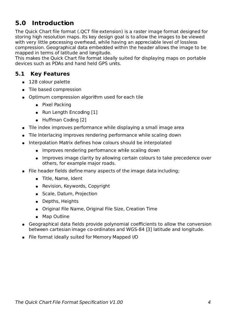
5.0 IntroductionThe Quick Chart file format (.QCT file extension) is a raster image format designed for storing high resolution maps. Its key design goal is to allow the images to be viewed with very little processing overhead, while having an appreciable level of lossless compression. Geographical data embedded within the header allows the image to be mapped in terms of latitude and longitude.This makes the Quick Chart file format ideally suited for displaying maps on portable devices such as PDAs and hand held GPS units.

5.1 Key Features

● 128 colour palette

● Tile based compression

● Optimum compression algorithm used for each tile

● Pixel Packing

● Run Length Encoding [1]

● Huffman Coding [2]

● Tile index improves performance while displaying a small image area

● Tile Interlacing improves rendering performance while scaling down

● Interpolation Matrix defines how colours should be interpolated

● Improves rendering performance while scaling down

● Improves image clarity by allowing certain colours to take precedence over others, for example major roads.

● File header fields define many aspects of the image data including;

● Title, Name, Ident

● Revision, Keywords, Copyright

● Scale, Datum, Projection

● Depths, Heights

● Original File Name, Original File Size, Creation Time

● Map Outline

● Geographical data fields provide polynomial coefficients to allow the conversion between cartesian image co-ordinates and WGS-84 [3] latitude and longitude.

● File format ideally suited for Memory Mapped I/O


6.0 Quick Chart File Layout

Offset Size (Bytes) Content

0x0000 24×4 Meta Data - 24 Integers/Pointers

0x0060 40×8 Geographical Referencing Coefficients - 40 Doubles

0x01A0 256×4 Palette - 128 of 256 Colours

0x05A0 128×128 Interpolation matrix

0x45A0 w×h×4 Image Index Pointers

- - File Body - Text strings and compressed image data

6.1 Data Formats

Integers are stored as 4 bytes in Little-Endian [4] byte order.

Pointers are stored as 4 bytes in Little-Endian byte order and refer to byte locations relative to the beginning of the file.

Doubles are stored as 8 byte IEEE-754 [5] double precision format.

Strings are stored as 1 byte per character in ASCII [6] and are NULL terminated.

Palette colours are stored as 3 bytes + 1 padding byte (Blue, Green, Red, 0x00).


6.2 Meta Data

Offset Data Type Content

0x00 Integer Magic Number0x1423D5FE - Quick Chart Information0x1423D5FF - Quick Chart Map

0x04 Integer File Format Version

0x08 Integer Width (Tiles)

0x0C Integer Height (Tiles)

0x10 Pointer to String Long Title

0x14 Pointer to String Name

0x18 Pointer to String Identifier

0x1C Pointer to String Edition

0x20 Pointer to String Revision

0x24 Pointer to String Keywords

0x28 Pointer to String Copyright

0x2C Pointer to String Scale

0x30 Pointer to String Datum

0x34 Pointer to String Depths

0x38 Pointer to String Heights

0x3C Pointer to String Projection

0x40 Integer Bit-field FlagsBit 0 - Must have original fileBit 1 - Allow Calibration

0x44 Pointer to String Original File Name

0x48 Integer Original File Size

0x4C Integer Original File Creation Time (seconds since epoch)

0x50 Integer Reserved, set to 0

0x54 Pointer to Struct Extended Data Structure (see section 6.2.1)

0x58 Integer Number of Map Outline Points

0x5C Pointer to Array Map Outline (see section 6.2.2)


6.2.1 Extended Data Structure


0x00 Pointer to String Map Type

0x04 Pointer to Array Datum Shift (see section 6.2.3)

0x08 Pointer to String Disk Name

0x0C Integer Reserved, set to 0


0x14 Integer Serial Number? (Optional)


0x1C Integer Reserved, set to 0

6.2.2 Map Outline

The Map Outline is an array of latitude/longitude pairs which mark out the boundary of the mapped region. The size of this array is stored in the Meta Data area at offset 0x58. Most maps will have four points to mark out the four corners of the map. Aerial photographs can have several hundred points to mark out the boundaries of counties.


0x00 Double Latitude

0x08 Double Longitude

... ... ...

6.2.3 Datum Shift

The datum shift is a pair of latitude/longitude values indicating the offset on the co-ordinates for this map.


0x00 Double Datum Shift North

0x08 Double Datum Shift East


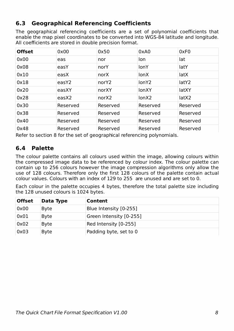
6.3 Geographical Referencing Coefficients

The geographical referencing coefficients are a set of polynomial coefficients that enable the map pixel coordinates to be converted into WGS-84 latitude and longitude. All coefficients are stored in double precision format.

Offset 0x00 0x50 0xA0 0xF0

0x00 eas nor lon lat

0x08 easY norY lonY latY

0x10 easX norX lonX latX

0x18 easY2 norY2 lonY2 latY2

0x20 easXY norXY lonXY latXY

0x28 easX2 norX2 lonX2 latX2

0x30 Reserved Reserved Reserved Reserved



0x48 Reserved Reserved Reserved ReservedRefer to section 8 for the set of geographical referencing polynomials.

6.4 Palette

The colour palette contains all colours used within the image, allowing colours within the compressed image data to be referenced by colour index. The colour palette can contain up to 256 colours however the image compression algorithms only allow the use of 128 colours. Therefore only the first 128 colours of the palette contain actual colour values. Colours with an index of 129 to 255 are unused and are set to 0.

Each colour in the palette occupies 4 bytes, therefore the total palette size including the 128 unused colours is 1024 bytes.


0x00 Byte Blue Intensity [0-255]

0x01 Byte Green Intensity [0-255]

0x02 Byte Red Intensity [0-255]

0x03 Byte Padding byte, set to 0


6.4.1 Interpolation Matrix

Since the images stored in Quick Chart format are relatively large, it is often necessary to view them scaled down. To improve the clarity of the scaled down image, interpolation is required. However due to the size of the image, and the fact that a palette is used, this process would require a high processing overhead.

The solution to this problem is to use a matrix of pre-calculated colour indices. To determine the palette index of two interpolated colours, use the two colours as a row and column index of the interpolation matrix.

The image in figure 1 represents an example content of an interpolation matrix. An extra row of pixels has been added to the top and left to show the original colours. The matrix has a line of symmetry about the leading diagonal. Also notice how the colours of the matrix are biased away from background colours towards the colours of major map features such as grid lines (blue), roads (blue, pink, orange and yellow) and text (black). This biasing allows these features to remain visible as the image is scaled down, preserving the clarity of the map.

Interpolation matrix data are stored as a block of 16384 bytes, one byte per colour as 128 rows of 128 colours. The offset of any given row/column index into this matrix can be determined by;

Offset=128×y x

Symmetry of the matrix allows interchangeability of the x and y variables.

6.5 Image Index

The image is compressed using tiles of 64x64 pixels. The image dimensions in terms of the number of tiles are stored in the Height and Width Meta data fields. For each tile in the image, an entry is present in the index. Each index entry is a pointer to the compressed image data for the tile. Each pointer is four bytes in size, hence the size of the image index can be calculated as follows;

Index Size=4×width×height

The offset of any given tile in the index can be calculated by;

Offset=4×Width×y x


Figure 1: Interpolation Matrix

7.0 Compressed Image DataEach tile within the image is compressed to reduce the size of the image file. Three compression algorithms are used to compress the image data, and all three algorithms rely on the fact that an image tile will likely contain fewer colours than the overall image. By using a sub-palette, the number of bits required to reference a given colour can be reduced.

● Pixel Packing

Not strictly a compression technique, a more efficient method for storing tiles that have few colours.

● Run Length Coding

More effective on tiles where a few colours are repeated many times.

● Huffman Coding

An entropy encoding algorithm, useful for complex tiles where some colours occur much more frequently than others.

The pixel packing and run length coding algorithms use the first byte of the compressed data to determine the number of colours in the sub-palette. The encoding of this first byte of compressed data enables it to also be used to determine the compression algorithm used by a tile, as follows;

If b0==0 or b0==255 then tile is Huffman coded.

Else If b0127 then tile is Pixel Packed.

Else tile is Run Length coded.

7.1 Interlacing

The pixel content of each tile is scanned from left to right in rows of 64 pixels. The rows however are not in top to bottom order. Instead they are interlaced using a bit-reverse sequence. The decompressed tile data must be scanned out row at a time using this row sequence;

Original Row Binary Reverse Binary Destination Row

0 000000 000000 0

1 000001 100000 32

2 000010 010000 16

3 000011 110000 48

4 000100 001000 8

5 000101 101000 40

... ... ... ...This interlacing scheme reduces the overheads while viewing an image at scaled down resolutions. For example, if an image was to be displayed at a scale down of 1:2, it would be desirable to take every other row of each tile. With this interlacing scheme, to display all of the even rows, only the first half of the tile data needs to be decompressed. This works for all scale down factors, eg for 1:4, only the first ¼ of the tile data needs to be decompressed.


7.2 Pixel Packing

Pixel packing is an efficient method for storing tile data where the number of colours used in the tile is low. A sub-palette is created for the colours used within the tile, and the number of bits required per pixel is determined from the size of the sub-palette. For example, if a tile had 13 colours, 4 bits would be required in order to address the colours of the sub-palette.

256 - Subpal Size

Colour Colour Colour Colour Colour ... Packed Tile Data

Packed Tile Data

Packed Tile Data

Packed Tile Data

Packed Tile Data

Packed Tile Data

Packed Tile Data

Packed Tile Data

... ...

The first byte codes for the size of the sub-palette;

Sub-Palette Size=256−b0

Following this is the sub-palette with one byte per colour index. Each sub-palette byte is a colour index for the main image palette. The tile image data immediately follows the sub-palette.

Tile image data are stored in blocks of 4 bytes. The colours are then packed into the block of 4 bytes, aligned to the LSB of the first byte. Any remaining space within the 4th

byte that is too small to fit another pixel is not used. For example, if a tile has a sub-palette of 7 colours, 3 bits would be required per pixel. Therefore 10 pixels (30 bits) of data can be packed into the 4 byte block, leaving 2 unused bits. In this case, a total of 410 blocks (1640 bytes) of data would be required in order to store the 64x64 pixel tile.

7 Byte 0 0 7 Byte 1 0 7 Byte 2 0 7 Byte 3 0

3 3 2 2 2 1 1 1 6 5 5 5 4 4 4 3 8 8 8 7 7 7 6 6 X X 10 10 10 9 9 9

The number of bits required to store the colour is determined from the sub-palette size.

7.3 Run Length Coding

Run length coding compresses image data where a single colour is repeated multiple times. By using a sub-palette similar to the pixel packing technique, the number of bits required to reference a colour is reduced, leaving the remaining bits of the byte to be used for specifying the repeat count.

Subpal Size

Colour Colour Colour Colour Colour ... Repeat Count / Colour

Repeat Count / Colour







... ...

The first byte codes for the size of the sub-palette. However with run length coding, the number does not need to be subtracted from 256.

Following this is the sub-palette with one byte per colour index. Each sub-palette byte is a colour index for the main image palette. The tile image data immediately follows the sub-palette.

Compressed data are stored as a stream of bytes, with the sub-palette index right aligned to the LSB and the repeat count stored in the remaining bits. For example, if a tile only used 4 colours, the 4 colour sub-palette would only require a 2 bits in order to address each colour. This leaves 6 bits to be used to specify the repeat count, giving maximum of 63 repeats.

7 Run-length Encoded Byte 0

REP5 REP4 REP3 REP2 REP1 REP0 COL1 COL0

The number of bits required to store the colour depends only upon the sub-palette size.


7.4 Huffman Coding

Huffman coding is the most complex of the three coding methods. A special sub-palette called a code book is used to reduce the number of bits per pixel, however the binary codes used to reference the colours of the sub-palette have varying lengths. Short code words are given to colours that occur most frequently, and the longest code words are given to colours that occur least frequently.

During the compression process, the tile is analysed to determine the frequency of occurrence of each colour. A Huffman tree is then created by sorting the frequencies in order of occurrence, and leafs and branches are assigned systematically such that the most frequently occurring colours have the shortest route from the root node to the leaf. The method produces an optimised Huffman tree which can then be transformed into a codebook with varying code lengths for compressing the tile image data.

To decompress the tile, the same codebook created for the compression process must used. Image data are treated as a continuous bit stream and as each bit is read, the codebook is used to determine which direction to take at a certain branch of the Huffman tree. Once a leaf node is reached, the colour for the current pixel has been determined, codebook pointer is returned to the root node of the tree and execution of the bit stream sequence continues.

0x00or0xFF

Code Book Data

Code Book Data

Code Book Data

Code Book Data

Code Book Data

Code Book Data

... Bit Stream Data

Bit Stream Data

Bit Stream Data

Bit Stream Data

Bit Stream Data

Bit Stream Data

Bit Stream Data

... ...

7.4.1 Huffman Codebook

The codebook is stored in such a way that it resembles the Huffman tree. Each entry in the codebook is either a branch or a colour. A simple test can determine if a codebook entry bn is a branch or a colour;

If bn128 then bn is a colour index from the main palette.

Else bn is a branch.

Codebook branches are essentially a relative 'goto' instruction. The branch entry contains the destination address relative to the current position in the code book. Codebook branches always jump forwards in the codebook and one of take two forms, near or far. With near branches, the relative jump destination is within 127 bytes of the jump origin. Far branches can have jump destinations up to 65536 bytes away from the jump origin. In reality, it is unusual to have a far jump much above 200 for a tile of 64x64 pixels. If a codebook entry bn is a branch, then the type and relative jump distance of the branch can be calculated as follows;

If bn128 then the branch is of type near.

Relative Jump=257−bn

If bn==128 then the branch is of type far.

Relative Jump=65537−256×bn2bn12

Note that the far jump requires an additional 2 bytes of space in the codebook.


7.4.2 Huffman Bit Stream

Image data are packed into a continuous binary stream beginning in the LSB of each byte. As each bit is read from the bit stream, the Huffman tree within the codebook section is traversed in a similar manner as the execution of a finite state machine. At each branch in the tree, the bit read from the bit stream determines whether or not to follow the branch, or continue;

● 0 - Do not follow the branch, continue to the next entry.

● 1 - Follow the branch.

As soon as a colour is encountered in the codebook, the colour is output for the current pixel, and the codebook pointer must be reset to the beginning of the codebook.

The process should be stopped after the last pixel of the tile has been drawn.

7.4.3 Finding the Start of the Bit Stream

In order to find the start of the bit stream, a codebook tree scan must be performed.

Since every branch in the tree splits two ways, there will always be one more colour than the total number of branches. By scanning through the codebook, counting the number of branches, and the number of colours. The end of the codebook is at the point where the number of colours found exceeds the number of branches found.

The end of the codebook is the beginning of the bit stream.

7.4.4 Exceptions

One exception to the normal Huffman decoding procedure is the case where no branches exist in the codebook.

In this case the codebook just contains a single colour connected to the root node. The tile is therefore a blank square filled with this colour, and no bit stream is present.


7.4.5 Huffman Coding Example

To decode the following compressed data;

00 F7 FF 54 FF 34 FF 1D FF 53 2F 1B AC 4F D5 10 00 29 ...

First parse through, identifying the sub-palette colours and and branches, then identify the beginning of the bit stream using the technique described in section 7.4.3;

Code Book Data Bit Stream Data

00 F7 FF 54 FF 34 FF 1D FF 53 2F 1B AC 4F D5 60 8E 27 ...

Example sub-palette mapping;

Palette Index

Example Colour

0x54 Red

0x34 Green

0x1D Blue

0x53 Magenta

0x2F Cyan

0x1B Yellow

The Huffman codebook can then be checked for out of bounds branch jumps by verifying that all jumps fall within the codebook. The codebook could also be checked to verify that only one route leads to any given branch or colour. Refer to figure 2 for a diagrammatic representation of the codebook.

From section 7.4.1:

0xF7 decodes as a relative jump forwards of 10 bytes.

0xFF decodes as a relative jump forwards of 2 bytes.


Figure 2: Diagrammatic Representation of Huffman Codebook

0 0 0 0 01 1 1 1 1

F7 FF 54 FF 34 1D 53 2F 1BFF FF

The Huffman tree represented by this codebook can then be drawn, refer to figure 3.

From the Huffman tree, the variable length codes that represent each colour can be easily identified.

Palette Index

Example Colour

Huffman Code

0x54 Red 00

0x34 Green 010

0x1D Blue 0110

0x53 Magenta 01110

0x2F Cyan 01111

0x1B Yellow 1

The bit stream can then be decompressed by processing one bit at a time until each colour has been decoded. Using the example bit stream data;

Bit Stream Data

AC 4F D5 60 8E 27 ...

Expanding the bit stream (from left to right);0 0 1 1 0 1 0 1 1 1 1 1 0 0 1 0 1 0 1 0 1 0 1 1 0 0 0 0 0 1 1 0 0 1 1 1 1 0 0 0 1 1 1 0 0 1 0 0

Decoded colours0 0 1 1 0 1 0 1 1 1 1 1 0 0 1 0 1 0 1 0 1 0 1 1 0 0 0 0 0 1 1 0 0 1 1 1 1 0 0 0 1 1 1 0 0 1 0 0

Therefore 23 pixels have been compressed into 6 bytes.

Due to the method by which the codebook is stored, the decompression algorithm does not need to extract and build the Huffman tree for each tile. After verifying the integrity of the codebook, the branches of the Huffman tree can be followed by evaluating it “in situ” while processing the bit stream, refer to figure 2.


Figure 3: Huffman Tree

0

1

1

0

0

1 0

1 0

1

8.0 Geographical Referencing PolynomialsIn order to convert image pixel coordinates into WGS-84 longitude and latitude, a three stage polynomial expansion is performed. The image coordinates x and y are relative to the top left corner of the image.

The set of polynomial coefficients and their location within the file was discussed in section 6.3.

R=lonX2×x2lonY2×y2

lonX×xlonY×ylonXY×x×ylon

S=latX2×x2latY2×y2

latX×xlatY×ylatXY×x×ylat

T=easX2×R2easY2×S2

easX×ReasY×SeasXY×R×Seas2×x

U=norX2×R2norY2×S2norX×RnorY×SnorXY×R×Snor2×y

Longitude=lonX2×T2lonY2×U2

lonX×TlonY×UlonXY×T×Ulon

Latitude=latX2×T2latY2×U2latX×TlatY×UlatXY×T×Ulat

Where:

x is the pixel horizontal coordinate from the left

y is the pixel vertical coordinate from the top

Longitude is the converted WGS-84 longitude

Latitude is the converted WGS-84 latitude

Finally, the datum shift east and north values from the meta data must be added to the converted longitude and latitude respectively in order to complete the conversion process.


the quick chart (.qct) file format specification0x08 double datum shift east the quick chart file...

Documents