the rand corporation - economia.uniandes.edu.co · cyclical nature of pricing, and the possibility...

The RAND Corporation

Theories of Cartel Stability and the Joint Executive CommitteeAuthor(s): Glenn EllisonSource: The RAND Journal of Economics, Vol. 25, No. 1 (Spring, 1994), pp. 37-57Published by: Blackwell Publishing on behalf of The RAND CorporationStable URL: http://www.jstor.org/stable/2555852Accessed: 18/11/2008 22:21

Your use of the JSTOR archive indicates your acceptance of JSTOR's Terms and Conditions of Use, available athttp://www.jstor.org/page/info/about/policies/terms.jsp. JSTOR's Terms and Conditions of Use provides, in part, that unlessyou have obtained prior permission, you may not download an entire issue of a journal or multiple copies of articles, and youmay use content in the JSTOR archive only for your personal, non-commercial use.

Please contact the publisher regarding any further use of this work. Publisher contact information may be obtained athttp://www.jstor.org/action/showPublisher?publisherCode=black.

Each copy of any part of a JSTOR transmission must contain the same copyright notice that appears on the screen or printedpage of such transmission.

JSTOR is a not-for-profit organization founded in 1995 to build trusted digital archives for scholarship. We work with thescholarly community to preserve their work and the materials they rely upon, and to build a common research platform thatpromotes the discovery and use of these resources. For more information about JSTOR, please contact [email protected].

The RAND Corporation and Blackwell Publishing are collaborating with JSTOR to digitize, preserve andextend access to The RAND Journal of Economics.

http://www.jstor.org

http://www.jstor.org/stable/2555852?origin=JSTOR-pdf

http://www.jstor.org/page/info/about/policies/terms.jsp

http://www.jstor.org/action/showPublisher?publisherCode=black

RAND Journal of Economics

Vol. 25, No. l, Spring 1994

Theories of cartel stability and the Joint Executive Committee

Glenn Ellison*

This article reexamines the experience of the Joint Executive Committee, an 1880s railroad cartel, to assess the applicability of the Green and Porter (1984) and Rotemberg and Saloner (1986) theories of price wars. After discussing necessary modifications to the theories, I estimate a number of dynamic models to explore the causes of price wars, the cyclical nature of pricing, and the possibility that secret price cuts may have been given. The estimates provide some support for the predictions of the first theory.

1. Introduction

* The "Joint Executive Committee" (JEC) was a railroad cartel organized in 1879 to set prices for transport between Chicago and the East Coast. Over the next seven years the cartel was only partially successful, with rates stable at $7 or $8 per ton in some years and occasional price wars pushing rates as low as $2.50 per ton in others. One thing the cartel did do very well was to keep detailed records, and as a result the JEC has proved to be a valuable setting in which to study the workings of a cartel (MacAvoy, 1965; Ulen, 1979; Porter, 1983b). In light of the previous literature, I will not review the history of the cartel here and recommend the accounts of MacAvoy and Porter to anyone unfamiliar with its situation.

Much of the more recent attention paid to the JEC is attributable to interest in game- theoretic models of collusion. Green and Porter's (1984) analysis of collusion with imperfect observation demonstrated that price wars need not be indicative of a failure to collude; they are, in fact, a necessary part of optimal collusive arrangements. The debate was further energized by the work of Rotemberg and Saloner (1986), whose alternate description of price wars is often regarded as at odds with that of Green and Porter. Pro- ponents of each theory have cited the JEC's experience as lending empirical support. (Por- ter, 1983b; Lee and Porter, 1984; Rotemberg and Saloner, 1986). Although the JEC has received a great deal of attention, I shall argue that the existing literature allows only a fairly incomplete assessment of the applicability of the Green and Porter and Rotemberg and Saloner theories. In an attempt to provide a more complete picture I shall reexamine the JEC, discussing at length the implications of the theories given the situation of the JEC and performing a number of empirical tests.

* Harvard University. I would like to thank Sara Fisher Ellison, Drew Fudenberg, Wally Mullin, Danny Quah, Julio Rotemberg,

and Jean Tirole for their comments and suggestions. Special thanks are due to Rob Porter both for his helpful suggestions and for providing me with the data used in this article.

Copyright@) 1994, RAND 37

38 / THE RAND JOURNAL OF ECONOMICS

The first theory considered here, that of Green and Porter, has been the primary focus of most previous studies. These studies have provided convincing evidence that price wars did occur in the JEC. The core content of the theory, however, is not just that price wars should occur in equilibrium, but that price wars should occur because firms follow particular strategies to sustain collusion, strategies in which price wars are triggered by random demand shocks. To evaluate this prediction within the context of the JEC, it is important to note that a variety of trigger strategies could have been used to sustain a nearly optimal outcome and that these strategies may be somewhat different from those in the text of Green and Porter (1984). For example, firms might react to unusual market share patterns or begin a price war whenever demand is unusually high (as opposed to low). The empirical analysis focuses on the transition probabilities in a switching regressions model (incorporating elements from the models of Porter (1983b), Cosslett and Lee (1985), and Hajivassiliou (1989)) to see whether any such trigger strategies were used. Some evidence for this is found.

The second theory considered, that of Rotemberg and Saloner (1986), is commonly associated with the statement that price wars are more likely to occur during booms, and therefore viewed as somehow in opposition to the Green and Porter theory. The actual Rotemberg and Saloner model, however, is really about countercyclical pricing-firms have perfect information and adjust prices smoothly in response to demand conditions. In contrast, the JEC was a cartel with imperfect information because secret price cuts were possible. When adapted to such a situation, the Rotemberg and Saloner analysis might predict either countercyclical pricing or price wars during booms. Interestingly, these predictions may be applied not only to booms in the traditional sense, but also to the seasonal pattern in the JEC's demand. Here, however, the empirical evidence provides little support for the theory.

Finally, the article considers a simple but heretofore unexplored prediction common to each of these theories, that firms should not cheat on their agreements. The discussion of secret price cutting requires the estimation of a set of more complicated hidden regime models, and stresses the problems of interpretation inherent in such models. While some cheating apparently occurred, it appears to have been fairly rare. This may be taken as further supporting the Green and Porter theory to the extent that we would expect rational firms to have cheated if the proper dynamic incentives to cooperate were not maintained.

2. The Green and Porter theory

* Theory and previous results. Green and Porter (1984) first formalized the observation that collusion is possible with imperfect information in a model of repeated Cournot competition between identical firms. They assume production levels are unobservable, and that there is noise in demand. Firms do observe the market price, and therefore receive an imperfect signal of their competitors' behavior. What Green and Porter show is that a degree of collusion can be sustained via trigger strategies that involve switches between collusive periods and price wars. In a collusive period, the firms produce at a point between the Cournot and monopoly levels. In a price war, the firms produce at the Cournot level. The optimal degree of collusion is sustained by trigger strategies in which firms produce at the collusive level until the market price falls below a specified level, at which point a price war begins. Abreu, Pearce, and Stachetti (1986) extend the analysis by allowing for more general strategies and show that an equilibrium involving two states and trigger strategies is indeed optimal.

In two important respects the JEC differs from the classic Green and Porter formu- lation. First, it is certainly more reasonable to think of the railroads not as setting quantities, but rather as setting prices with reputations for quality of service and differing route structures creating differentiated demands. Second, what is and is not observable is also

ELLISON / 39

different. Given the possibility of secret price cuts and with no single market price, price is not observable. On the other hand, the JEC did collect quantity data that presumably were reliable.'

In developing predictions applicable to the JEC, it is probably best not to push too far the analysis of optimal equilibria. With asymmetric firms and observable market shares, the optimal equilibrium may well resemble those of Fudenberg, Levine, and Maskin (1993), where full collusion is supported by equilibria that specifically punish deviators. If we tried to apply such a theory, however, we would be immediately faced both with the reality that no asymmetric punishments were observed and with limitations in the amount of data available to identify complex strategies. Even restricting ourselves to symmetric trigger strategies, what is optimal may also be hard to determine without knowing far more details than are available.

If we ask instead what simple, nearly efficient equilibria are possible, we can find a number of plausible triggers upon which an equilibrium might be based. The best signal of cheating with observable market shares would likely be some pattern of a high market share for one firm with lower market shares for all the rest. A second possible signal is high aggregate demand, as when one or more firms lower prices there is not only a transfer of market shares but also an expansion of demand. (This contrasts with the low aggregate demand that causes price wars in the literal Green and Porter model.) Finally, if we wished to find an equilibrium robust to some type of coalition-proofness notion, it might make sense for firms to react to an unusually low market share of one firm, because a firm will experience unusually low sales when one or several other firms cheat.

In trying to assess whether the organization of the JEC resembles any of these equilibria, we may test several predictions. First, price wars should occur. Second, price wars should occur precisely when random demand shocks resemble a signal like those noted above. Finally, firms should not cheat and offer secret price cuts. I defer any further discussion of this last issue until the final section.

The previous empirical work on the JEC has largely concerned the first of these predictions. Porter (1983b) first showed that the data are indicative of multiple supply regimes with prices were reduced by about 40% during price wars. Cosslett and Lee (1985) noted further that the price wars do indeed appear to be continuous rather than a randomly scat- tered set of weeks. Lee and Porter (1984), Berry and Briggs (1988), and Hajivassiliou (1989) provide additional evidence on the existence of price wars.

While central to the theory, the second prediction has been addressed only in Porter (1985). Perhaps further work has been discouraged by Bresnahan's (1989) observation that with only six to eleven price wars to work with, we have much less data on such dynamic issues. Porter uses a two-step approach in which a collusion indicator is first estimated by maximum likelihood and then regressed on a measure of deviations of market shares from the assigned quotas over the sample of collusive periods. While Porter does not find significant evidence of such a trigger, we cannot conclude that no trigger exists. There are many reasonable triggers for which Porter does not look. In addition, the two- step approach is perhaps susceptible to a loss of power because the onset of price wars may be misclassified in the first stage. Interestingly, Porter does find that large aggregate demand (he does not test residuals) does appear to cause price wars. In his framework, however, it is not possible to tell if this is a trigger strategy or related to Rotemberg and Saloner's predictions.

ra Model and data. The models of this article are all based on that of Porter (1983b). The primary difference is that I impose a Markov structure related to those of Cosslett

Some support for this assumption is provided by the cartel's consideration of plans in which the shipment data were to be used to determine side payments by firms exceeding allotments.


and Lee (1985) and Hajivassiliou (1989) on the transitions between the cooperative and price war regimes. I test whether collusion was maintained by trigger price strategies by focusing on the determinants of the probability with which a price war begins.

The structural model described below follows Porter's specification very closely, so it will only be sketched here. The reader may refer to Porter (1983b) for motivation and interpretation of the parameters. The demand for grain shipments is assumed to be given by

log Qt = ao + a, log P, + a2 LAKES, + 3-14SEASXX, + U1,, (1)

where SEASXX, and LAKES, are intended to capture seasonal variation in demand and the effect of the opening and closing of the Great Lakes to navigation. In a departure from Porter's model, I will usually assume that U1, follows an AR(1) process,

Ult = pult-1 + Vit I PI<'.1 (2)

The supply curve, also as in Porter, is assumed to have the form

log Pt = 030 + 131 log Qt + /2It + 03-6 DMxt + U2t, (3)

where It is an indicator of collusion, and the DMx are four dummy variables for changes in the cartel composition. The errors V1t and U2t are assumed to have a multivariate normal distribution. The possibility of secret price cuts makes Pt unobservable, but we do have available the official prices firms were supposed to have charged. Although using this series could introduce an errors-in-variables problem, the optimal cartel theory predicts that firms should in fact never deviate from the official prices, so we can hope that these errors are small.

As mentioned above, I use a Markov structure on the transitions to detect causes of price wars. Specifically, I assume that the indicator It of collusion evolves according to the logit model

eYW' Prob{I+ I= It, Zt} =J +eew) (4)

where Zt is the set of predetermined variables at time t. Taking Wt to be a constant independent of It gives a standard model with independent regime switches, as in Porter (1 983b). Allowing Wt to contain It adds a Markov structure to the price wars, as in Cosslett and Lee (1985), so that a noncooperative state today can be likely to lead to another noncooperative state next week. I shall also include several other variables in Wt to test the predictions of the Green and Porter model. Note that the specification differs from that of Hajivassiliou (who does not test for Green and Porter-style triggers) in that variables are modelled as affecting transition probabilities, i.e., the probability of starting a price war, not the probability of being in a given state.

Estimates of the parameters are computed by maximizing the joint likelihood of the structural equations and of the path of transitions. Hopefully, the simultaneous maximi- zation will allow the model to date more accurately the start of price wars and provide more power in detecting triggers than would a two-step approach. The computation is similar to that of Cosslett and Lee (1985). I use numerical derivatives to compute robust standard errors for all estimators.

The data for the article are those compiled by Ulen (1979) and later used by Porter (1983b). The data contain weekly observations on quantity, price, and other variables over a 328-week period from 1880 to 1886. Table 1 gives summary statistics.

QUANTITY gives the total eastbound grain shipments of the railroads in the JEC in tons per week. PRICE is given in dollars per 100-pounds of grain. The LAKES variable is a dummy variable set to one when the Great Lakes were navigable and steamers could

ELLISON / 41

TABLE 1 Summary Statistics

Variable Mean Standard Deviation Minimum Maximum

QUANTITY 25384 11632 4810 76407 PRICE .2465 .0665 .125 .400 LAKES .5732 .4954 0 1 DM1 .4238 .4949 0 1 DM2 .0457 .2092 0 1 DM3 .4329 .4962 0 1 DM4 .0152 .1227 0 1 BIGSHARE1 1.0908 .5690 .0397 2.9711 BIGSHARE2 1.2409 .7102 .1849 4.2345 BIGSHAREQ 1.1744 .5162 .1578 2.9728 SMALLSHARE 1.2303 .7373 .1161 5.7565

compete with the railroads. The four structural dummies DM1-DM4 mark significant changes in the membership of the cartel. Seasonal dummy variables labelled SEAS1-SEAS12 are used for the first twelve four-week periods of each year. All of these variables are exactly as in Porter (1983b).

In addition, I created four more complicated variables to test the Green and Porter model. The variables are admittedly ad hoc, and they represent a rough attempt to capture a few of the possible workings of a cartel. The variable BIGSHARE1 is intended to be a plausible trigger in a cartel that switches to a price war when one firm obtains a suspi- ciously high market share. The measure is based on deviations in log qi, rather than qi, so that differing punishment probabilities will not disturb the proportionality between gains from a given increase in log qi, related to a price cut and losses from a subsequent price war. Recognizing that the measure is arbitrary, it seemed prudent to construct two variants on the theme, BIGSHARE2 and BIGSHAREQ. Each of the variables is the largest amount by which the strength si, of any firm's demand exceeds its predicted value Sit (after nor- malizing by the sample standard deviation), i.e., each is of the form maxi(si, - JIt)/oi. In

1 the case of BIGSHARE1 and BIGSHAREQ, sit = log qi, - - E log qj, is used to represent

n X the strength of firm i's demand. In the case of BIGSHARE2, the ordinary market share is used. The predicted values Sit used in constructing BIGSHARE1 and BIGSHARE2 are taken to be the average of the same measure for the previous twelve weeks. The predicted value for BIGSHAREQ is computed from the assigned quota. While the use of quotas as ex- pectations initially seems appealing, in practice the quotas were often set unrealistically, hence deviations will not accurately reflect deviations from adherence to a uniform price.2 Adjustments to the predictions had to be made at the start of the series and as the cartel structure shifted. A fourth variable, SMALLSHARE1, is intended to be a plausible trigger for a cartel in which price wars are triggered by an unusually small market share for one firm. Using the same measures as in BIGSHARE1, it is the largest amount by which the strength of any firm's demand falls short of its predicted value.

E Results. In this subsection I present first a "standard" model much like those that previous studies have used to identify price wars. Subsequently, I explore the causes of price wars. The results of the "standard" model are given in the left half of Table 2. The model differs from that of Porter (1983b) in two ways. First, it allows for serial correlation in the demand equation. The effect of this change can be seen by comparing the two halves of the table. Note that the coefficient U1,_1 is highly significant and several other coef-

2 For example, MacAvoy (1965) reports that the Chicago and Grand Trunk Railway was admitted with a 10% quota while receiving only a 2-7% share at the cartel price.


TABLE 2 The "Standard" Model

Demand: logQ, = a0 + a, log P, + a2 LAKES, + a3_14 SEASXX, + U1. Price: logP, = [30 + [l3 logQ, + /32 I, + [33-6 DMx, + U2,

eyWt Regimes: Prob {I,+, = 1 I,, Z} (1 + eyWt)

"Standard" Model No Serial Correlation

Variable Estimate Standard Error Estimate Standard Error

Demand CONSTANT 7.677 1.882 9.019 .361 log P -1.802 1.287 -.843 .193 LAKES -.009 .112 -.460 .348 SEAS1 -.103 .086 -.117 .157 SEAS2 .146 .145 .167 .180 SEAS3 .147 .138 .149 .166 SEAS4 -.011 .157 .145 .242 SEAS5 -.315 .165 .062 .164 SEAS6 -.550 .179 .077 .170 SEAS7 -.446 .198 .081 .176 SEAS8 -.504 .194 -1.116 .374 SEAS9 -.395 .165 .048 .185 SEAS10 -.545 .164 .102 .191 SEAS11 -.521 .180 .085 .304 SEAS12 -.397 .173 .183 .241

Supply CONSTANT -4.764 1.863 -5.649 9.461 log Q .306 .178 .398 .928 DM1 -.154 .075 -.211 .124 DM2 -.246 .064 -.283 .160 DM3 -.317 .076 -.373 .242 DM4 -.198 .119 -.419 .422 It .637 .104 .660 .406

Regimes CONST. (I, = 1) 3.675 .474 3.661 .513 CONST. (I, = 0) -2.641 .404 -2.620 .476

Other cr. .290 .061 .396 .029 0'12 -.007 .004 -.045. .142 0C2 .160 .045 .191 .313 U,,_, 1.832 .085

Log-likelihood 181.0 37.2

ficients change. Most importantly, the estimated price elasticity increases from .84 to 1. 80, indicating that the JEC did indeed face an elastic demand curve. As a consequence, Por- ter's approximation 0 to the degree of collusion increases from .40 to .85, indicating that the JEC was much more aggressive in its pricing than has been previously reported. (A value of one would indicate full monopoly pricing.) The second change is the incorporation of a Markov structure for the transition probabilities. Consistent with a number of previous studies, the regimes are not independently determined with collusion having probability .975 (e3.67/(1 + e3.67)) after a collusive state and .067 after a price war state. On the whole, the model reinforces the view of the JEC as setting prices collusively between occasional price wars, suggesting a greater degree of collusion than has been claimed in the past.

I now turn to the second prediction described above, trying to infer whether price wars resulted from the use of Green and Porter-style trigger strategies by examining the causes of price wars. The results of six models are summarized in Table 3. Each model contains all of the variables of the "standard" model plus an additional variable (or two)

ELLISON /43

TABLE 3 Causes of Price Wars

eywt Regimes: Prob{JI,? I 1 It 1, Zt} _ (1 + eywt)

Model

Parameter 1 2 3 4 5 6

CONSTANT 4.63 4.36 3.95 2.96 4.43 4.35 (.77) (.77) (1.30) (.66) (.81) (.90)

BIGSHARE1 - .77 (.49)

BIGSHARE2 - .46 (.39)

BIGSHAREQ -.21 (1.06)

SMALLSHARE .66 (.89)

Vt -4.15 -5.00 (2.64) (3.15)

Ut 1.17 (1.15)

*Note: Estimated standard errors in parentheses.

that affects the probability of a transition from a collusive to a price war state. For each variable, the theory predicts a larger value to be more likely to lead to a breakdown of collusion. The coefficient estimates are then expected to be negative. Because the "standard" model indicates that there are only six price wars, we should not expect high significance levels. (There are no substantial changes in the structural parameters of the models. Hence, only the logit parameters for the transition to a price war are reported.)

The first model in the table focuses on what should be the best signal of cheating, that of one firm obtaining an unusually high market share. The coefficient estimate on the BIGSHARE1 variable is negative as predicted, and is significant at the 6% level in a one- tailed test. The next two columns of the table give estimates from models with the two other variants on this variable, BIGSHARE2 and BIGSHAREQ. The estimates are again negative, but they are smaller and not significant. The fourth model includes the SMALLSHARE variable to test whether price wars are triggered by an unusually low demand for one firm. The coefficient estimate has the wrong sign and is not significant. The fifth model tests whether large residuals VI, in aggregate demand cause price wars. The coefficient is large and negative, as the theory predicts, and is again significant at the 6% level. The fact that two essentially orthogonal triggers appear to increase the probability of a price war is also suggestive of the possibility that each is imperfectly correlated with some true trigger that has a more powerful effect.

The sixth model in Table 3 takes advantage of the incorporation of serial correlation to sharpen the interpretation of the previous result. In the Green and Porter theory, unanticipated demand shocks cause price wars. In the Rotemberg and Saloner theory, price wars are more likely when demand is high and anticipated to decline (see the next section).- That the unanticipated component of demand, V1t, is significant while the full demand shock Ult is not allows us to distinguish between these explanations in favor of that of Green and Porter where Porter (1985) could not.

It is important to remember that the causes of price wars have been estimated from very few examples. The timing of these price wars is also not clear, with the "standard" model above not matching the onset date of Ulen's (1979) classification for any of the price wars. For this reason, it is advisable to worry about whether the results above are ve-ry sensitive to the timing of the regimes,. Table 4 presents, the, rslsof simple logit


TABLE 4 Price War Causes Using Reported Regimes

eYWt Regimes Prob{J,+ = 1 J, = 1, Zo} = (1 + eYWt)

Model

Parameter 1 2 3 4

CONSTANT 3.68 3.55 3.25 2.92 (.65) (.65) (.61) (.57)

BIGSHARE1 -.71 (.46)

BIGSHARE2 -.51 (.39)

BIGSHAREQ -.33 (.44)

SMALLSHARE .05 (.37)

* Note: Estimated standard errors in parentheses.

models that attempt to predict the probability of the onset of a price war in Ulen's classification, J. The results are surprisingly similar to those of the previous table, providing further evidence of the existence of a Green and Porter-type trigger and perhaps suggesting that with a better classification the results would be stronger.

Although the results described above support the applicability of the Green and Porter theory, I would like to point out that they are not completely positive. In a Green and Porter cartel it is not sufficient for a signal of cheating to increase the likelihood of a price war. It must be the case that the relationship is strong enough to deter firms from cheating. Absent data on costs and firm-specific elasticities, we can give only a very rough calculation of whether the proper incentives are maintained. Suppose that firm i offers a secret price cut in period t and raises its demand by 10%. If the price cut that induces this response is small, profits in period t may be increased by, say, 8-10%. How large is the strategic disincentive to cheat given the estimated effect of BIGSHARE1? The measure of demand, maxk(log qk, - 1/n E log qj,)/ok, would be expected to be increased by

j log(1. l)/loi whenever firm i would otherwise have had the highest market share deviation. A simple computer simulation with reasonable parameter values gives the probability of a price war increasing by about .001. If the losses from a price war are about 15 times the per-period profits, the future loss is about 1-2% of current profits. The effect we have estimated is then several times too small to support collusion, and cannot be much larger given the precision of our estimates.

There are a number of possible explanations for this result. First, it is quite possible that we have significantly underestimated the responsiveness of the data to signals of cheating. This could happen because the firms have information not contained in our data, because imperfect price data induce misclassifications of the onset of price wars, and/or because a true trigger for price wars is only imperfectly correlated with BIGSHARE1. On the other hand, it could also be simply that the responses of the JEC were not sufficiently strong to deter cheating in a noncooperative equilibrium. While the results of this section support the applicability of the Green and Porter theory, it cannot be said that collusive equilibrium strategies have been clearly identified.

3. The Rotemberg and Saloner theory

* Theory and previous results. The Rotemberg and Saloner model of collusion with time-varying demand is often misinterpreted simply as implying that price wars are likely

ELLISON / 45

to break out during booms. While this is understandable given the title of the article, the Rotemberg and Saloner model has no uncertainty about past actions, and therefore has no price wars in the sense of the dramatic regime shifts of the Green and Porter model. Instead the theory is really one of countercyclical pricing, or more precisely, countercyclical de- grees of collusion in the sense that firms set prices further from the monopoly level when demand is high than when it is low. The intuition for this is simple. Suppose firms are not very patient so that they are just able to deter cheating at a specified price. If demand in the current period is then increased relative to demand in the future, the gain from cheating will be increased relative to the cost of an ensuing punishment. In order to elim- inate an incentive to cheat, the price must be lowered.

To apply rigorously the ideas of Rotemberg and Saloner's model to the JEC, it would be necessary to add time-varying demand to a Green and Porter-style model with unobservable prices. The optimal equilibrium of a model with imperfect observation is in one sense a very natural place to apply Rotemberg and Saloner's ideas because the incentive constraints do bind. Hence firms' incentives to cheat must be reduced whenever demand is expected to decline. However, in adapting a cartel design to a situation of declining demand, a variety of changes are possible. Prices in each phase may be raised or lowered, price wars may be lengthened or shortened, and the sensitivity of triggers may be adjusted. Prices will be countercyclical if the optimal adjustment involves lowering prices when demand is low, and price wars will be more common during booms if the optimal adjustment makes triggers more sensitive (or if the cartel fails to sufficiently re- duce the incentive to cheat). In the absence of a formal analysis, it is possible to appeal to the literature by regarding booms as analogous to a lowering of firms' discount factors. The numerical solutions reported in Porter (1983a) then suggest that we should expect both countercyclical prices and more price wars during booms, although the results may be sensitive to such assumptions as the distribution of the error terms. In fairness to the Rotemberg and Saloner theory, it should be pointed out that the analysis is probably more applicable to situations less complicated than the one described above. While the effects do appear in the optimal equilibrium regardless of complexity, we could easily imagine that a nineteenth-century railroad cartel would instead choose a design with prices somewhat below the maximum possible, but in which prices and punishment thresholds need not be fine-tuned to the vagaries of each week's demand.

To apply the theory it is also necessary to reexamine what a "boom" means. A boom in the theory is a period when high current demand will be followed by a period of lower demand during an ensuing price war (Haltiwanger and Harrington, 1991). In the case of the JEC, we can identify two situations in which current demand is likely to be significantly higher than the future demand (with "future" here meaning the next fifteen or so weeks). First, given the serial correlation of demand shocks that has been estimated, a large random component of demand yesterday leads to increased demand today with less than a proportional increase in the future. This effect is closely related to the standard view of booms, and it justifies the conclusion without the assumption that demand shocks are observable in advance. Second, we have the entirely new interpretation that there may be a seasonal pattern to collusion. In the winter, when the Great Lakes were closed, the JEC received much higher demand. The incentive to deviate is thus at its peak just before the lakes are to melt. Given the parameter estimates of our standard model, each of the two effects should be of approximately the same strength. To summarize, an analysis of the applicability of the Rotemberg and Saloner theory should assess whether prices are less collusive or price wars are more likely to occur during booms, where booms are redefined as noted above.

Only two previous articles, those of Rotemberg and Saloner (1986) and Hajivassiliou (1989), have considered the Rotemberg and Saloner theory in the context of the JEC, and neither directly addresses any of the predictions outlined above. Rotemberg and Saloner


attempt only a rough look at annual frequencies of price wars and note that price wars are more common in years in which grain production is high and the Great Lakes remain frozen for a long time. These variables, however, do not identify situations in which demand is higher than it is expected to be in the next few months. Using only annual data, price wars also cannot be tied to the conditions of the week in which a price war begins. Hajivassiliou similarly considers only an index of grain production, and his analysis concerns not whether this index tends to cause price wars, but rather whether it tends to be high during price wars. No previous work has explored countercyclical pricing in the JEC.

11 Model. Conceptually, modifying the model of Section 2 to test the predictions of the Rotemberg and Saloner model is fairly simple. A variable B, that measures the ratio of current to future demand should be added in in two places. To test whether B, makes price wars more likely we can simply add B. to the logit model for the transition probability Prob {II, = 1 I I, = 1, Zj. To test whether prices are less collusive when B, is high we can use the modified supply equation

logPt,= 30 + (31 logQt + f32It + f33BtIt + f4-7DMxt + U2t.

A negative coefficient on /3 would indicate prices that are less collusive during booms. In trying to perform such a test, the only difficulty lies in the determination of an

appropriate variable B. To combine the effects of serially correlated shocks and seasonal factors I take Bt not to be any observable, but rather a function of the predetermined variables and parameters. The primary function used for this purpose is

BOOM, = K X 52 exp(a2LAKESt + a3-14SEASXX, + PUlt-1) BOM 52-.

Pwt+s -Pc,t+s) exp(a2LAKESt+s + a3-14SEASXXt+s + ps+lUlti1)

The expression represents a ratio of present demand to the expected future demand during the course of a subsequent price war. Here, the parameters a2 through a14 and p are those being simultaneously estimated while the value P - P is the additional probability of being in a price war s periods after one begins implied by the results of the standard model.3

To further analyze the effect of booms, I will also separate the effects of serially correlated errors and seasonal variation. To analyze the first, I simply include Ujt_,It in the supply equation and Ult in the transition probability. Among the possible effects tested, the occurrence of price wars when U1l is large is most similar to the common interpretation of the Rotemberg and Saloner model as implying price wars during booms. To look at seasonal variation, I create a function similar to that used for the combined effect,

exp(a2LAKESt + a3-14SEASXXt) SEASONALt = KX -52-.

(Pw,t+s -Pc,t+s) exp(a2LAKESt+s + a3-14SEASXXt+s) s=1

Results. While we might have expected that finding countercyclical levels of collusion would be easy given that it is not hampered by the small number of price wars, the results on the Rotemberg and Saloner model are somewhat disappointing, and we can make few firm conclusions given the imprecision of the estimates. The first set of columns in Table 5 gives the results of the estimation of a model in which the combined measure BOOM, affects the level of collusion and the likelihood of a price war. The estimate of

3 These latter values are not estimated simultaneously, as doing so would require a fixed point calculation to overcome the circularity of BOOM, depending on Pv,+s, which is in turn a function of BOOM,. It is hoped that this will not unduly bias the estimates and standard errors.

ELLISON / 47

TABLE 5 Effect of Booms

Demand: logQ, = a0 + a, logP, + a2 LAKES, + a3,4 SEASXX, + U, Price: logP, = go + /, logQ, + 132 I, + /33 B,I, + /34_7 DMx, + U2,

Regimes: Prob{I,+, = 1 j I Z'} = (1 + eyWt)

Combined Effect Demand Shocks Seasonal

Variable Estimate Standard Error Estimate Standard Error Estimate Standard Error

Demand CONSTANT 7.319 3.060 7.964 1.345 8.016 1.970 logP -1.996 2.055 -1.594 .898 -1.574 1.459 LAKES -.041 .127 -.036 .133 .008 .110 SEAS1 -.149 .181 -.045 .104 -.065 .125 SEAS2 .151 .155 .164 .139 1.136 .191 SEAS3 .236 .170 .080 .193 .124 .298 SEAS4 .100 .239 -.065 .185 -.048 .254 SEAS5 -.206 .279 -.312 .173 -.318 .181 SEAS6 -.451 .287 -.445 .207 -.513 .392 SEAS7 -.335 .283 -.298 .264 -.385 .504 SEAS8 -.371 .328 -.314 .330 -.440 .577 SEAS9 -.227 .426 -.265 .238 -.338 .416 SEAS1O -.340 .445 -.444 .185 -.531 .243 SEAS1 1 -.370 .297 -.478 .158 -.524 .203 SEAS12 -.311 .195 -.162 .162 -.403 .174

Supply CONSTANT -6.856 6.801 -6.186 3.415 -4.419 2.545 log Q .517 .673 .450 .335 .274 .250 DM1 -.223 .148 -.205 .090 -.164 .087 DM2 -.303 .179 -.302 .106 -.257 .070 DM3 -.437 .314 -.402 .148 -.326 .103 DM4 -.238 .130 -.319 .104 -.234 .197 I, .758 .416 .712 .195 .622 .119 BOOM,!, -.233 .428 U,,_ I, -.156 .164 SEAS,!, .041 .417

Regimes CONST. (I,= 1) 3.596 .474 4.604 .775 3.925 1.241 BOOM, (I, = 1) .446 1.582 U,,(I, = 1) -.777 .477 SEAS, (I, = 1) -2.786 7.704 CONST. (I, = 0) 2.624 .404 -2.620 .390 -2.677 .546

Other 0, .301 .061 .280 .041 .278 .064

0-12 - .018 .023 - .017 .013 - .007 .004 0?2 .204 .045 .187 .079 .155 .046 U,,_, .838 .085 .831 .078 .824 .063

Log-likelihood 186.2 187.1 181.2

the coefficient of BOOMtlt in the supply equation indicates a countercyclical degree of collusion in pricing, with an implied decrease of about 3% in the collusive price when the incentive to deviate is one standard deviation above the mean. However, the standard error is almost twice this large. As a result, we cannot reject that collusion is procyclical or that the reduction is 12%. It appears that this boom effect is hard to separate econo- metrically from the effect of quantity on price. The second and third sets of columns examine the decomposition into seasonal and demand shock components in hopes that the models will be more precisely estimated or that we might gain confidence from a coin- cidence of estimates. The estimate of the countercyclical response to demand shocks is


TABLE 6 Causes of Price Wars

eYWI Regimes: Prob{I, , = 1 1, = 1, Z,} = + e'lw)

Model

Parameter 1 2 3

CONSTANT 3.64 4.35 3.87 (.49) (.90) (.71)

BOOM, .36 (1.48)

U1, 1.17 (1.15)

SEASONAL, -2.51 (3.50)

V,, -5.00 (3.15)

Note: Estimated standard errors in parentheses.

more precise, though still not significant, indicating a 5% drop in prices when U1,1 is one standard deviation above the mean. No evidence at all is found for countercyclical price responses to seasonal cycles.

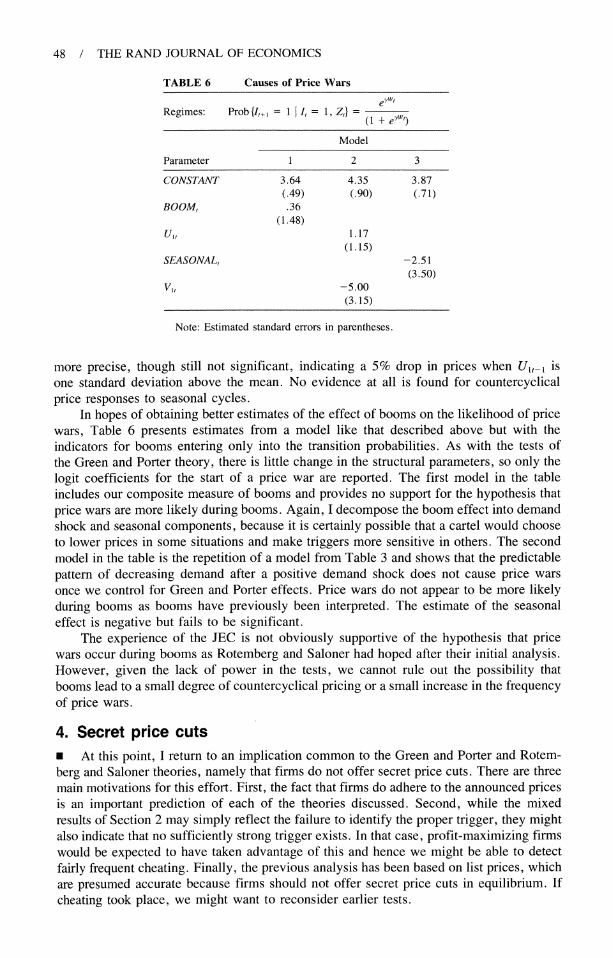
In hopes of obtaining better estimates of the effect of booms on the likelihood of price wars, Table 6 presents estimates from a model like that described above but with the indicators for booms entering only into the transition probabilities. As with the tests of the Green and Porter theory, there is little change in the structural parameters, so only the logit coefficients for the start of a price war are reported. The first model in the table includes our composite measure of booms and provides no support for the hypothesis that price wars are more likely during booms. Again, I decompose the boom effect into demand shock and seasonal components, because it is certainly possible that a cartel would choose to lower prices in some situations and make triggers more sensitive in others. The second model in the table is the repetition of a model from Table 3 and shows that the predictable pattern of decreasing demand after a positive demand shock does not cause price wars once we control for Green and Porter effects. Price wars do not appear to be more likely during booms as booms have previously been interpreted. The estimate of the seasonal effect is negative but fails to be significant.

The experience of the JEC is not obviously supportive of the hypothesis that price wars occur during booms as Rotemberg and Saloner had hoped after their initial analysis. However, given the lack of power in the tests, we cannot rule out the possibility that booms lead to a small degree of countercyclical pricing or a small increase in the frequency of price wars.

4. Secret price cuts * At this point, I return to an implication common to the Green and Porter and Rotem- berg and Saloner theories, namely that firms do not offer secret price cuts. There are three main motivations for this effort. First, the fact that firms do adhere to the announced prices is an important prediction of each of the theories discussed. Second, while the mixed results of Section 2 may simply reflect the failure to identify the proper trigger, they might also indicate that no sufficiently strong trigger exists. In that case, profit-maximizing firms would be expected to have taken advantage of this and hence we might be able to detect fairly frequent cheating. Finally, the previous analysis has been based on list prices, which are presumed accurate because firms should not offer secret price cuts in equilibrium. If cheating took place, we might want to reconsider earlier tests.

ELLISON / 49

There are no standard theoretical predictions about the nature of secret price cuts other than that they should not occur. Secret price cuts are also by nature not recorded in the JEC data. Given this combination, I should warn the reader that this section will be quite speculative. I would also like to mention that given reports in the contemporary trade press, it is very likely that some price cutting occurred.4 The real goal of this section is to see whether we can obtain some idea of the frequency and magnitude of such behavior so that we may comment on its implications. With these caveats, I move on to discuss methodology.

Suppose a secret price cut were offered only once for one week. An econometrician, like the JEC members, would have no chance of finding it. On the other hand, if periods of both price cutting and strict adherence to the official price are common, there is hope. In this case, it is as if secret price cutting is a significant omitted variable in the demand equation, shifting demand upward relative to that expected given the official price. Mo- tivated by this observation, I follow a two-step approach. First, I examine the demand equation in the JEC for evidence of omitted variables. Subsequently, when the presence of such variables is indicated, I ask whether they may indeed reflect secret price cuts.

E Looking for secret price cuts via hidden regimes. The problem of identifying secret price cuts is in many ways similar to that of identifying collusive and noncollusive behavior. In Section 2, collusion was identified by functional form assumptions-the residuals in the supply equation were assumed to be normal while collusive price increases are assumed in accordance with the Green and Porter theory to have a distribution with a two- point support. Here, such an approach is probably less appropriate given the lack of a theory describing the distribution of price cuts. If price cuts are normally distributed, they cannot be identified. It is probably true, though, that price cuts are not normally distributed, but instead have a mass point on no cut being offered with some continuous distribution over small positive price cuts. The approach taken here is simply to look for the easiest thing to find, a distribution of price cuts with a small finite support. Such price cuts would appear in the data as occasional shifts in demand relative to the official price. As the whole exercise is doomed if there is no evidence of any omitted variables in demand, I will look for such shifts first and worry later about whether they are secret price cuts.

To formally explore the possibility that omitted variables shift demand, I apply a model of hidden regimes with Markov transitions that is more complicated and somewhat more far-fetched than that of Section 2. Essentially, I add indicator variables for one or two additional demand regimes to the demand relation (1). The model I refer to as model 2 allows for two demand regimes so that the demand equation is

logQ, = ao + a, logP, + a2LAKES, + a3-14SEASXX, + a15REGIME1, + U1,. (5)

I intend for REGIME1 to be an indicator for periods of price cuts, so I assume that this high-demand state occurs with probability Pi whenever firms are trying to collude, but never occurs during price wars when firms are already presumably pricing at marginal cost.

Model 3 allows for three demand regimes so that the demand equation becomes

log Q, = a0 + a, logP, + a2 LAKES, + a3-14 SEASXX,

+ a15 REGIME 1t + al6 REGIME2t + U1l. (6)

4The Daily Commercial Bulletin of June 16, 1881, contains a typical report: "Some agents claim to insist on 20c Grain to New York, while others state that 15c has no doubt been accepted." An article from February 2, 1886, expresses more confidence: "There is little doubt but rates are being cut on shipments of Grain to the East by one or two lines."


FIGURE 1

Collusion REGIME1 d nw

REGIMEl |High demand It=l1 Collusion REGIME2 dand

REGIME1 HighdemLowdemand NEl ------------------- As--------------------7-----------------

rice 1ar TEmE deman

AanI am eniinn thatME -11E il ea nictrfra ihdmndrgm u to ecrt pic cus.helowestdemand rgm ih ersn eido nsal o

REGIME3 Collusion I X I I

REGIME2 rc1a

~~~~~~~Hihdemand Pi osvr etelbrpolmunsal o tasi aeec si

isnt= crca REIM the prollusio athan , I ilnttytPrvd2a nepeainfrti

Med. demand p-GIME a/

REGIME3 Low demand i L Jyf fir

probabgain Isamenvs ing tha t REGIMEP 1ini r ahigem regime due

tod secrt prie cuts.eTh lwowrgiest-deandregimhte smigh reprtiesna perbaiodtiof unusull lowlsv

.~ ~~Md deman

demand due to s Prie war r pric.si Figure 1 illu timeste stuture Timex tastiosi oes2ad3 Time larg is not crucial to the problem at hand, I will not try to provide an interpretation for this

regime. In a collusive state, I assume that the high demand REGIMEr1 arises with probability PI, the medium-demand REGIME2 with probability P2, and the third regime with probability 1 - (PI + P2)F I again assume that REGIME1 never arises during a price war and that the other two regimes occur with the same relative probabilities under collusive and price war pricing.

Figure 1 illustrates the structure of regiae transitions in models 2 and 3. The large boxes represent the different regimes possible at time t. In model 2, there are two regimes with collusive prices (the two possible demand regimes) and one with competitive prices. The arrows indicate probabilistic transitions and are labelled with the probabilities with which they are taken. For example, the high-demand REGIME 1 occurs with probability pI, and the low-demand REGIME2 occurs with probability 1 - PI whenever the firms are colluding. Within each of the regimes, prices and quantities are determined by the supply and demand relations (3) and (5), with the appropriate values of the regime dummies, e.g., with REGIME1t = 1 and It = 1 within the uppermost period-t state in the figure. The diagram for model 3 is similar, but with the five states representing the three possible demand regimes under collusive pricing and the two possible demand regimes in a price war.

The estimation of these models is almost unreasonably successful. Maximum-likelihood estimates are reported in Table 7. Most structural parameter estimates are quite similar to those of our standard model. Many of the key parameters, including the price

ELLISON / 51

TABLE 7 Estimates of Hidden Regimes

Demand: logQ, = a0 + a, logP, + a2 LAKES, + a314 SEASXX, + a15 REGIMEI, + a16 REGIME2, + U1, Price: logP, = go3 + f,3 logQ, + 132 I, + 03-6 DMx, + U2,

Model 2 Model 3

Variable Estimate Standard Error Estimate Standard Error

Demand CONSTANT 8.147 .870 7.651 .176 logP -1.354 .711 -1.587 .092 LAKES -.222 .073 -.229 .092 SEAS1 -.046 .122 -.114 .087 SEAS2 .166 .147 .163 .095 SEAS3 .016 .115 .106 .108 SEAS4 .056 .137 -.041 .122 SEAS5 -.225 .169 -.321 .127 SEAS6 -.271 .158 -.374 .162 SEAS7 -.163 .194 -.139 .159 SEAS8 -.350 .205 -.332 .157 SEAS9 -.179 .182 -.184 .167 SEAS1O -.215 .122 -.219 .148 SEAS1 1 -.194 .121 -.089 .128 SEAS12 -.216 .083 -.091 .114 REGIME1 .439 .036 .728 .027 REGIME2 .384 .022

Supply CONSTANT -3.861 1.577 -4.101 .412 log Q .220 .153 .242 .038 DM1 -.165 .069 -.162 .072 DM2 -.244 .062 -.239 .068 DM3 -.331 .069 -.323 .063 DM4 -.228 .082 -.198 .119 1, .595 .079 .608 .047

Transition probabilities q,23 .979 .012 .976 .037 qo .061 .028 .070 .076 Pi .650 .071 .256 .083

P2 .519 .086 Other

a-l .121 .015 .089 .006 U12 - .001 .001 - .0002 .0007 02 .097 .021 .099 .011 Utl .888 .031 .947 .018

Log-likelihood 529.0 582.5

elasticity of demand and the effect of collusion on prices, are more significant, particularly in model 3. There is also a truly dramatic increase in fit relative to the standard model, with an improvement in log-likelihood similar to that reported by Porter when he first added a second supply regime to the model. The most striking result is the extremely high degree of significance of the dummy variables REGIME1 for the hidden demand regimes we were looking for. The t-statistics on the REGIME1 parameter estimates, 12.1 and 26.7 in models 2 and 3 respectively, are almost unreasonably high given a sample size of 328 weeks. In model 2, the high-demand REGIME1 has demand increased by about 55%. In model 3, the high-demand REGIME1 has demand 41% above the level of the medium- demand REGIME2, while the low-demand regime will have demand 32% below that of REGIME2.

At this point, I think it is important to caution the reader that it is not claimed that we have estimated the effect of secret price cuts. The high-demand regimes of the two


FIGURE 2

.6

.5

.4

.3

.2

0 -.87 -.69 -.52 -.35 -.17 0 .17 .35 .52 .69 .87

models are very different, with that of model 2 occurring in 65% of the periods and that

of model 3 occurring in 26% of them: Clearly, at least one model is finding evidence of

something other than price cutting. I conclude only that there is very strong evidence of

significant omitted variables in the demand equation. To help understand these results it is instructive to look at the demand residuals of

the standard model. If no price cuts were given, these might appear to be normally dis-

tributed. If occasional price cuts of the same magnitude were given, the distribution would

have an additional peak shifted to the right by an amount equal to the demand response

to a price cut of the given magnitude. Figure 2 presents a kernel density estimate of the

residuals V1t from the standard model. I think the reader will agree that the residuals do

not appear to be normally distributed. The smaller peak to the right resembles the predicted

effect of price cutting and is the empirical regularity that accounts for the high-demand REGIME1 in model 3.

O Do the estimated regimes look like secret price cuts? The fact that I have so far

ignored the problem of interpreting the results of the previous model should not be taken

to imply that I do not see it as important. To the contrary, I wish to emphasize strongly

that the reported results could easily be attributed to a number of other factors (e.g.,

weather, irregular schedules, steamship competition, mechanical problems) or simply to

departures from the functional form or distributional assumptions. I believe that the inter-

pretation of models with hidden regimes is an important and often overlooked question and therefore I discuss it at some length in this section.

Secret price cuts are just one of a number of possible explanations for our findings,

and we cannot claim to know much about many of the alternate explanations. We cannot

then simply perform hypothesis tests of competing theories to decide among them. Instead,

I will try to provide a number of small analyses to see whether the omitted variables have

the properties we would expect of secret price cuts. The first type of evidence I consider is that which has been most common in other

studies-a simple look at the reasonableness of the parameter estimates. For example,

Porter (1983b) compares the magnitude of his estimated supply shift to the prediction that

"collusive" supply shocks would increase prices by something less than, but of the same

magnitude as, the difference between monopoly and competitive prices. We have little

ELLISON / 53

theory to go on. Perhaps the best standard for comparison we have is obtained from reports in the contemporary trade press which indicate that perhaps 10-25% is a reasonable size for price cuts. As far as the frequency of price cuts goes, we can only say that the fact that the cartel went as long as two years between price wars suggests that price cuts were not too common.

In model 2, the high-demand REGIME1 occurs with estimated probability fr = .65 when firms are colluding. Given the estimated price elasticity of 1.35, a regime shift of the indicated magnitude would only result from price cuts of between 25% and 30%. It seems unlikely that price cuts of this size could have occurred so often without clear historical evidence and more frequent price wars. I think that this alone is sufficient evidence to conclude that the high-demand regime of model 2 does not reflect secret price cutting, and will examine the regimes in this model no further. In model 3, the high- demand REGIME1 occurs with estimated probability fr = .26. Given the estimated price elasticity of 1.59, the increase in demand from REGIME2 to REGIME1 would require a price cut of about 20%. This certainly seems like a reasonable size and frequency for price cuts, although given our lack of precise predictions about price cutting and alternative explanations, we cannot be much more confident that we have found the effect of price cuts.

The second type of evidence I would like to consider is the relationship between the demand shifts I have found and the available historical evidence on price cutting. The argument can be thought of as analogous to Porter's use of the similarity between his estimates and Ulen's reported regimes to justify the price war interpretation. In the case of secret price cuts, two relationships to the historical data might be envisioned. First, if secret price cuts cannot be kept completely secret, we might expect the high-demand regime to be accompanied by simultaneous reports in the press of price cutting. Such reports are likely to be highly inaccurate, however, because shippers who receive special treatment will want to keep it secret to maintain their advantage in the grain market, and those who do not will gladly claim they did if it might trigger a price war. Second, to the extent that the JEC members believe such reports, whether true or not, we might expect also that secret price cutting will break out in the periods immediately following the reports.

Historical evidence on price cutting was compiled from the Chicago Board of Trade's Daily Commercial Bulletin, which contains both price quotes for rail freight transportation and occasional reports of rumored price cuts. Two indicator variables were created. The dummy variable CUTREPORTED is set to one in any week in which an article stated that secret price cuts were rumored to be given. The dummy variable CUTLISTED is set to one whenever the average of the daily prices listed in the newspaper was at least three cents below the official price. The two variables identify twelve and eighteen weeks respectively as involving price cuts.

Table 8 presents a simple descriptive analysis of the relationship between the maximum-likelihood classification of weeks into demand regimes and three potential indicators of collusion: the two noted above and Ulen's series of reported price wars. Each row gives the frequency with which the appearance of the indicator at time t is accompanied by the occurrence of the high-demand regime in periods t through t + 5. The fractions are computed over the sample of periods for which periods t and t + s both involve collusive pricing. Entries marked with an asterisk indicate that the high-demand regime is significantly more common when the indicator occurs than in the rest of the sample.6 (Remem- ber, about 26% of all periods involve the high-demand regime.) The first two columns of

5 Some such reports appear in the Daily Commercial Bulletin of June 16, 1881, September 25, 1884, and January 22, 1885.

6 The standard errors have been computed conditional on the regime classification, not taking the estimation of the regimes into account.


TABLE 8 Historical Evidence on Secret Price Cuts

Indicator of Price Cuts (C,)

CUTREPORTED CUTLISTED Reported Price War

E(REGIME1 | Cr, I) .44 .30 .25

E(REGIMElt+1 C,, I,+) .57* .13 .28

E(REGIMEl,+2 |C, I+2) .66* .33 .40*

E(REGIME1,+3 |C, I+3) .50 .40 .46*

E(REGIMEl,+4 C, It+4) .33 .60* .41*

E(REGIMElt+5 I C,, I+5) .20 .25 .34

* The high-demand regime is significantly more common when the indicator occurs than in the rest of the

sample.

the table are based on very small samples, so only very large differences will be significant.

In the first line of the table, we see that the indicators are slightly more likely to be accompanied by the appearance of the high-demand regime, though not significantly so. In the next several lines we see that the high-demand regime is much more likely to occur in the few weeks following the occurrence of reports of cheating, in accordance with the

speculation that firms might engage in retaliatory price cutting. The results of this section would likely be even stronger if it were not for the fact that one-third to one-half of the time a price war has begun within a month of the reports and hence the points are dropped from the frequency calculation in the lower rows of the table. Approximately 15% of the occurrences of the high-demand regime are directly attributable to excess occurrences of the high-demand regime following one of the price cutting indicators. All together, the table provides fairly convincing evidence that the high-demand regime estimates reflect, at least in part, secret price cutting.

If the JEC is in fact a Green and Porter-style cartel in which firms react to aggregate demand shocks, there is also a fairly direct test available of whether the hidden regimes are or are not observable to the JEC members. Absent Rotember and Saloner-type effects, we would expect that the trigger for a Green and Porter cartel would be based only on

demand shocks unobservable to the firms. If the demand regimes are perfectly observable, we would expect a trigger to be based on the residuals of the model, i.e., on V1t. If the

demand regimes are completely unobservable, an aggregate demand trigger would be based on the sum of the demand residual and the effect of the regime shift variables.

FIGURE 3

Collusion P

REGIME1 High demand Pi

/=1 REGIME2 Collusionp2

t ~~~~Med. demand q3

Collusion REG(ME3 Low demand

REGIME2 Price war 1-Pi Med. demand7

Ito 0 0

Price war Low demand

Time t-1 Time t Time t+1

ELLISON / 55

TABLE 9 Observability of Hidden Regimes

Demand: logQ, = a0 + a, logP, + a2 LAKES, + a3_14 SEASXX, + al5 REGIME 1, + al6 REGIME2, + U1, Price: logP, = goS + /31 logQ, + /32 I, + /33-6 DMx, + U2,

eywt Regimes: qj = yt W, (1 Vit R,)

(1 + eY ,)

Variable Estimate Standard Error

Demand CONSTANT 7.67 .48 log P -1.57 .43 LAKES -.23 .06 SEAS1 -.11 .04 SEAS2 .16 .12 SEAS3 .10 .13 SEAS4 -.04 .10 SEAS5 -.32 .09 SEAS6 -.38 .09 SEAS7 -.14 .10 SEAS8 -.33 .10 SEAS9 -.19 .11 SEAS1O -.22 .07 SEASl 1 -.09 .07 SEAS12 -.09 .06 REGIME1 .73 .04 REGIME2 .38 .05

Supply CONSTANT -4.07 .97 log Q .24 .09 DM1 -.16 .07 DM2 -.24 .06 DM3 -.32 .07 DM4 -.20 .07 I, .61 .07

Transition probabilities qi CONST. 5.65 1.06

qiVlt -3.17 1.26 qiRt -.48 1.03

qo .07 .03

P .26 .05

P2 .52 .07 Other

(r, .09 .01

O(l2 .0001 .001

072 *.10 .02 U1,-1 .947 .02

Log-likelihood 584.4

To test between these hypotheses, I estimate a model like model 3 but in which the transition from a collusive to a price war state is a function both of Vjt and of Rt- a15 REGIMEIt + ail6(REGIME2t- 1). Figure 3 illustrates the nature of the regime transitions in the model. The probabilities qj, q2, and q3 of continuing in a price war are all assumed to be determined by a single logit model with Vjt and Rt as explanatory variables. (Note that each of these quantities is dependent on the demand regime.) With completely unobserved regimes, Vjt and R, should have identical coefficients. With observed regimes, the coefficient on Rt should be zero. While it may seem completely unreasonable to suppose that we could identify the form of the trigger given that we could barely say that a trigger exists, the results in Table 9 do in fact yield significant results. At the 5%


level we can reject the equality of the coefficients on VI, and R, in the logit model of

transition probabilities. We therefore reject the idea that the regimes represent only factors

unobservable to the JEC members. To the contrary, the estimates suggest that the high-

demand regime is mostly due to factors the JEC recognized and which did not lead them

to initiate price wars. In this section we have seen that there are significant unobserved variables affecting

demand, and that one of these regimes present in one-quarter of all periods is compatible

with price cuts of about 20%. While there is historical evidence of price cutting correlated

with the estimated regimes, it is likely that secret price cutting accounts for only a fairly

small fraction of these periods. These findings are obviously not compatible with the pre-

diction of the theory that no cheating should take place, but also they are not indicative

of the JEC's having provided grossly inadequate incentives to cooperate. The results of

this section can also be seen as strengthening the conclusions of Section 2. Viewing the

model in Table 9 as one that partly corrects for the presence of omitted variables in de-

mand, we have found that aggregate demand shocks not only still appear to cause price

wars, but that the results are now clearly statistically significant.

5. Conclusion

* Previous work testing the Green and Porter theory has focused on the prediction that

price wars should occur. Using the familiar data on the Joint Executive Committee, this

is verified again here, with the traditional view challenged only in that I find prices to be

much closer to the monopoly level than has been previously reported. More importantly, I have used a model that focuses on the regime transition probabilities to provide evidence

for the existence of the trigger strategies that are central to the theory. Given the serially

correlated demand shocks, such trigger effects can be distinguished from the predictions

of the Rotemberg and Saloner model. The fact that several triggers are found to be sig-

nificant and significant results are also obtained using an alternate classification is sugges-

tive of the existence of a stronger mechanism than has been identified. The results are not completely positive, in that the initial estimates are not highly

significant and do not identify the presence of a mechanism sufficiently strong to deter

cheating. The literal prediction of the theory that no secret price cutting should occur also

appears to be false. The case for the existence of a stronger trigger is perhaps strengthened,

though, by the fact that cheating is not too widespread. In the context of cartels with imperfect observations, the Rotemberg and Saloner the-

ory has a number of new implications. In the case of the JEC, booms relevant to this

theory must be understood to be short-term demand shocks or seasonal peaks in demand.

Booms may lead to less collusive prices and/or more frequent price wars. I am unable to

find either of these effects, and in particular do not find evidence for the common inter-

pretation of price wars being more likely during booms. My estimates are disappointing in their lack of power, however, so moderate effects are certainly possible. In any case,

the JEC is also perhaps among the less likely places one would want to apply the Rotem-

berg and Saloner theory, so these results may not be reflective of the theory's applicability in other contexts.

References

ABREU, D., PEARCE, D., AND STACCHETTI, E. "Optimal Cartel Equilibria with Imperfect Monitoring." Journal

of Economic Theory, Vol. 39 (1986), pp. 251-269.

BERRY, S. AND BRIGGS, H. "A Non-parametric Test of a First-Order Markov Process for Regimes in a Non-

cooperatively Collusive Industry." Economic Letters, Vol. 27 (1988), pp. 73-77.

BRESNAHAN, T.F. "Empirical Studies of Industries with Market Power." In R. Schmalensee and R.D. Willig,

eds., The Handbook of Industrial Organization. New York: North-Holland, 1989.

ELLISON / 57

COSSLETT, S.R. AND LEE, L.F. "Serial Correlation in Latent Variable Models." Journal of Econometrics, Vol. 27 (1985), pp. 79-97.

Daily Commercial Bulletin. Chicago: Howard White & Co., 1880-1886. FUDENBERG, D., LEVINE, D., AND MASKIN, E. "The Folk Theorem with Imperfect Public Information." Mimeo,

Harvard University, 1993. GREEN, E.J. AND PORTER, R.H. "Noncooperative Collusion Under Imperfect Price Competition." Econometrica,

Vol. 52 (1984), pp. 87-100. HALTIWANGER, J. AND HARRINGTON, J.E. "The Impact of Cyclical Demand Movements on Collusive Behavior."

RAND Journal of Economics, Vol. 22 (1991), pp. 89-106. HAJIVASSILIOU, V. "Testing Game-theoretic Models of Price-fixing Behavior." Cowles Foundation Discussion

Paper no. 935, 1989. LEE, L.F. AND PORTER, R.H. "Switching Regression Models with Imperfect Sample Separation Information-

With an Application on Cartel Stability." Econometrica, Vol. 52 (1984), pp. 391-418. MAcAvoY, P.W. The Economic Effects of Regulation. Cambridge, Mass.: MIT Press, 1965. PORTER, R.H. "Optimal Cartel Trigger Price Strategies." Journal of Economic Theory, Vol. 29 (1983a), pp.

313-338. . "A Study of Cartel Stability: The Joint Executive Committee, 1880-1886. " Bell Journal of Economics,

Vol. 14 (1983b), pp. 301-314. . "On the Incidence and Duration of Price Wars." Journal of Industrial Economics, Vol. 33 (1985),

pp. 415-426. ROTEMBERG, J.J. AND SALONER, G. "A Supergame-Theoretic Model of Price Wars During Booms." American

Economic Review, Vol. 76 (1986), pp. 390-407. STIGLER, G.J. "A Theory of Oligopoly." Journal of Political Economy, Vol. 72 (1964), pp. 44-61. ULEN, T.S. Cartels and Regulation: Late Nineteenth Century Railroad Collusion and the Creation of the In-

terstate Commerce Commission. Ph.D., dissertation, Stanford University, 1979.

the rand corporation - economia.uniandes.edu.co · cyclical nature of pricing, and the possibility...

Documents