the random average process and random walk in a space-time
TRANSCRIPT

Digital Object Identifier (DOI) 10.1007/s00220-006-0036-yCommun. Math. Phys. 266, 499–545 (2006) Communications in
MathematicalPhysics
The Random Average Process and Random Walkin a Space-Time Random Environment in One Dimension
Márton Balázs1,�, Firas Rassoul-Agha2, Timo Seppäläinen1,��
1 Mathematics Department, University of Wisconsin-Madison, Van Vleck Hall, Madison, WI 53706, USA.E-mail: [email protected]; [email protected]
2 Mathematical Biosciences Institute, Ohio State University, 231 West 18th Avenue, Columbus, OH 43210,USA. E-mail: [email protected]
Received: 7 September 2005 / Accepted: 12 January 2006Published online: 9 May 2006 – © Springer-Verlag 2006
Abstract: We study space-time fluctuations around a characteristic line for aone-dimensional interacting system known as the random average process. The stateof this system is a real-valued function on the integers. New values of the function arecreated by averaging previous values with random weights. The fluctuations analyzedoccur on the scale n1/4, where n is the ratio of macroscopic and microscopic scales in thesystem. The limits of the fluctuations are described by a family of Gaussian processes.In cases of known product-form invariant distributions, this limit is a two-parameterprocess whose time marginals are fractional Brownian motions with Hurst parameter1/4. Along the way we study the limits of quenched mean processes for a random walkin a space-time random environment. These limits also happen at scale n1/4 and aredescribed by certain Gaussian processes that we identify. In particular, when we look ata backward quenched mean process, the limit process is the solution of a stochastic heatequation.
1. Introduction
Fluctuations for asymmetric interacting systems. An asymmetric interacting system isa random process στ = {στ (k) : k ∈ K} of many components στ (k) that influence eachothers’ evolution. Asymmetry means here that the components have an average drift insome spatial direction. Such processes are called interacting particle systems becauseoften these components can be thought of as particles.
To orient the reader, let us first think of a single random walk {Xτ : τ = 0, 1, 2, . . . }that evolves by itself. For random walk we scale both space and time by n because onthis scale we see the long-term velocity: n−1 X�nt� → tv as n → ∞, where v = E X1.The random walk is diffusive which means that its fluctuations occur on the scale n1/2, as
� M. Balázs was partially supported by Hungarian Scientific Research Fund (OTKA) grant T037685.�� T. Seppäläinen was partially supported by National Science Foundation grant DMS-0402231.

500 M. Balázs, F. Rassoul-Agha, T. Seppäläinen
revealed by the classical central limit theorem: n−1/2(X�nt� − ntv) converges weakly toa Gaussian distribution. The Gaussian limit is universal here because it arises regardlessof the choice of step distribution for the random walk, as long as a square-integrabilityhypothesis is satisfied.
For asymmetric interacting systems we typically also scale time and space by thesame factor n, and this is known as Euler scaling. However, in certain classes of one-dimensional asymmetric interacting systems the random evolution produces fluctuationsof smaller order than the natural diffusive scale. Two types of such phenomena have beendiscovered.
(i) In Hammersley’s process, in asymmetric exclusion, and in some other closelyrelated systems, dynamical fluctuations occur on the scale n1/3. Currently known rigor-ous results suggest that the Tracy-Widom distributions from random matrix theory arethe universal limits of these n1/3 fluctuations.
The seminal works in this context are by Baik, Deift and Johansson [3] on Ham-mersley’s process and by Johansson [19] on the exclusion process. We should pointout though that [3] does not explicitly discuss Hammersley’s process, but instead themaximal number of planar Poisson points on an increasing path in a rectangle. One canintrepret the results in [3] as fluctuation results for Hammersley’s process with a specialinitial configuration. The connection between the increasing path model and Hammers-ley’s process goes back to Hammersley’s paper [18]. It was first utilized by Aldous andDiaconis [1] (who also named the process), and then further in the papers [26, 28].
(ii) The second type has fluctuations of the order n1/4 and limits described by a familyof self-similar Gaussian processes that includes fractional Brownian motion with Hurstparameter 1
4 . This result was first proved for a system of independent random walks [30].One of the main results of the current paper shows that the n1/4 fluctuations also appearin a family of interacting systems called random average processes in one dimension.The same family of limiting Gaussian processes appears here too, suggesting that theselimits are universal for some class of interacting systems.
The random average processes (RAP) studied in the present paper describe a randomreal-valued function on the integers whose values evolve by jumping to random convexcombinations of values in a finite neighborhood. It could be thought of as a caricaturemodel for an interface between two phases on the plane, hence we call the state a heightfunction. RAP is related to the so-called linear systems discussed in Chapter IX of Ligg-ett’s monograph [22]. RAP was introduced by Ferrari and Fontes [14] who studied thefluctuations from initial linear slopes. In particular, they discovered that the height overthe origin satisfies a central limit theorem in the time scale t1/4. The Ferrari-Fontesresults suggested RAP to us as a fruitful place to investigate whether the n1/4 fluctuationpicture discovered in [30] for independent walks had any claim to universality.
There are two ways to see the lower order dynamical fluctuations.
(1) One can take deterministic initial conditions so that only dynamical randomness ispresent.
(2) Even if the initial state is random with central limit scale fluctuations, one canfind the lower order fluctuations by looking at the evolution of the process along acharacteristic curve.
Articles [3] and [19] studied the evolutions of special deterministic initial states ofHammersley’s process and the exclusion process. Recently Ferrari and Spohn [15] haveextended this analysis to the fluctuations across a characteristic in a stationary exclusionprocess. The general nonequilibrium hydrodynamic limit situation is still out of reachfor these models. [30] contains a tail bound for Hammersley’s process that suggests
Random Average Process 501
n1/3 scaling also in the nonequilibrium situation, including along a shock which can beregarded as a “generalized” characteristic.
Our results for the random average process are for the general hydrodynamic limitsetting. The initial increments of the random height function are assumed independentand subject to some moment bounds. Their means and variances must vary sufficientlyregularly to satisfy a Hölder condition. Deterministic initial increments qualify here asa special case of independent.
The classification of the systems mentioned above (Hammersley, exclusion, inde-pendent walks, RAP) into n1/3 and n1/4 fluctuations coincides with their classificationaccording to type of macroscopic equation. Independent particles and RAP are mac-roscopically governed by linear first-order partial differential equations ut + bux = 0.In contrast, macroscopic evolutions of Hammersley’s process and the exclusion pro-cess obey genuinely nonlinear Hamilton-Jacobi equations ut + f (ux ) = 0 that createshocks.
Suppose we start off one of these systems so that the initial state fluctuates on then1/2 spatial scale, for example in a stationary distribution. Then the fluctuations of theentire system on the n1/2 scale simply consist of initial fluctuations transported alongthe deterministic characteristics of the macroscopic equation. This is a consequence ofthe lower order of dynamical fluctuations. When the macroscopic equation is linear thisis the whole picture of diffusive fluctuations. In the nonlinear case the behavior at theshocks (where characteristics merge) also needs to be resolved. This has been done forthe exclusion process [25] and for Hammersley’s process [29].
Random walk in a space-time random environment. Analysis of the random averageprocess utilizes a dual description in terms of backward random walks in a space-timerandom environment. Investigation of the fluctuations of RAP leads to a study of fluc-tuations of these random walks, both quenched invariance principles for the walk itselfand limits for the quenched mean process. The quenched invariance principles havebeen reported elsewhere [24]. The results for the quenched mean process are included inthe present paper because they are intimately connected to the random average processresults.
We look at two types of processes of quenched means. We call them forward andbackward. In the forward case the initial point of the walk is fixed, and the walk runsfor a specified amount of time on the space-time lattice. In the backward case the initialpoint moves along a characteristic, and the walk runs until it reaches the horizontal axis.Furthermore, in both cases we let the starting point vary horizontally (spatially), and sowe have a space-time process. In both cases we describe a limiting Gaussian process,when space is scaled by n1/2, time by n, and the magnitude of the fluctuations by n1/4.In particular, in the backward case we find a limit process that solves the stochastic heatequation.
There are two earlier papers on the quenched mean of this random walk in a space-timerandom environment. These previous results were proved under assumptions of smallenough noise and finitely many possible values for the random probabilities. Bernabei[5] showed that the centered quenched mean, normalized by its own standard deviation,converges to a normal variable. Then separately he showed that this standard deviationis bounded above and below on the order n1/4. Bernabei has results also in dimension 2,and also for the quenched covariance of the walk. Boldrighini and Pellegrinotti [6] alsoproved a normal limit in the scale n1/4 for what they term the “correction” caused bythe random environment on the mean of a test function.

502 M. Balázs, F. Rassoul-Agha, T. Seppäläinen
Finite-dimensional versus process-level convergence. Our main results all state that thefinite-dimensional distributions of a process of interest converge to the finite-dimen-sional distributions of a certain Gaussian process specified by its covariance function.We have not proved process-level tightness, except in the case of forward quenchedmeans for the random walks where we compute a bound on the sixth moment of theprocess increment.
Further relevant literature. It is not clear what exactly are the systems “closely related”to Hammersley’s process or exclusion process, alluded to in the beginning of the Intro-duction, that share the n1/3 fluctuations and Tracy-Widom limits. The processes forwhich rigorous proofs exist all have an underlying representation in terms of a last-pas-sage percolation model. Another such example is “oriented digital boiling” studied byGravner, Tracy and Widom [16]. (This model was studied earlier in [27] and [20] underdifferent names.)
Fluctuations of the current were initially studied from the perspective of a movingobserver traveling with a general speed. The fluctuations are diffusive, and the limitingvariance is a function of the speed of the observer. The special nature of the characteristicspeed manifests itself in the vanishing of the limiting variance on this diffusive scale.The early paper of Ferrari and Fontes [13] treated the asymmetric exclusion process.Their work was extended by Balázs [4] to a class of deposition models that includes themuch-studied zero range process and a generalization called the bricklayers’ process.
Work on the fluctuations of Hammersley’s process and the exclusion process hasconnections to several parts of mathematics. Overviews of some of these links appearin papers [2, 10, 17]. General treatments of large scale behavior of interacting randomsystems can be found in [9, 21–23, 32, 33].
Organization of the paper. We begin with the description of the random average pro-cess and the limit theorem for it in Sect. 2. Section 3 describes the random walk in aspace-time random environment and the limit theorems for quenched mean processes.The proofs begin with Sect. 4 that lays out some preliminary facts on random walks.Sections 5 and 6 prove the fluctuation results for random walk, and the final Sect. 7proves the limit theorem for RAP.
The reader only interested in the random walk can read Sect. 3 and the proofs for therandom walk limits independently of the rest of the paper, except for certain definitionsand a hypothesis which have been labeled. The RAP results can be read independentlyof the random walk, but their proofs depend on the random walk results.
Notation. We summarize here some notation and conventions for quick reference. Theset of natural numbers is N = {1, 2, 3, . . . }, while Z+ = {0, 1, 2, 3, . . . } and R+ =[0,∞). On the two dimensional integer lattice Z
2 standard basis vectors are e1 = (1, 0)
and e2 = (0, 1). The e2-direction represents time.We need several different probability measures and corresponding expectation oper-
ators. P (with expectation E) is the probability measure on the space � of environmentsω. P is an i.i.d. product measure across the coordinates indexed by the space-time latticeZ
2. P (with expectation E) is the probability measure of the initial state of the randomaverage process. Eω is used to emphasize that an expectation over initial states is takenwith a fixed environment ω. Jointly the environment and initial state are independent, sothe joint measure is the product P ⊗ P. Pω (with expectation Eω) is the quenched pathmeasure of the random walks in environment ω. The annealed measure for the walks
Random Average Process 503
is P = ∫Pω
P(dω). Additionally, we use P and E for generic probability measuresand expectations for processes that are not part of this specific set-up, such as Brownianmotions and limiting Gaussian processes.
The environments ω ∈ � are configurations ω = (ωx,τ : (x, τ ) ∈ Z2) of vectors
indexed by the space-time lattice Z2. Each element ωx,τ is a probability vector of length
2M + 1, denoted also by uτ (x) = ωx,τ , and in terms of coordinates uτ (x) = (uτ (x, y) :−M ≤ y ≤ M). The environment at a fixed time value τ is ωτ = (ωx,τ : x ∈ Z).Translations on � are defined by (Tx,τω)y,s = ωx+y,τ+s .
�x� = max{n ∈ Z : n ≤ x} is the lower integer part of a real x . Throughout, Cdenotes a constant whose exact value is immaterial and can change from line to line.The density and cumulative distribution function of the centered Gaussian distributionwith variance σ 2 are denoted by ϕσ 2(x) and �σ 2(x). {B(t) : t ≥ 0} is one-dimen-sional standard Brownian motion, in other words the Gaussian process with covarianceE B(s)B(t) = s ∧ t .
2. The Random Average Process
The state of the random average process (RAP) is a height function σ : Z → R. It canalso be thought of as a sequence σ = (σ (i) : i ∈ Z) ∈ R
Z, where σ(i) is the height ofan interface above site i . The state evolves in discrete time according to the followingrule. At each time point τ = 1, 2, 3, . . . and at each site k ∈ Z, a random probabilityvector uτ (k) = (uτ (k, j) : −M ≤ j ≤ M) of length 2M + 1 is drawn. Given the stateστ−1 = (στ−1(i) : i ∈ Z) at time τ − 1, the height value at site k is then updated to
στ (k) =∑
j :| j |≤M
uτ (k, j)στ−1(k + j). (2.1)
This update is performed independently at each site k to form the state στ = (στ (k) :k ∈ Z) at time τ . The same step is repeated at the next time τ + 1 with new independentdraws of the probability vectors.
So, given an initial state σ0, the process στ is constructed with a collection {uτ (k) :τ ∈ N, k ∈ Z} of independent and identically distributed random vectors. These randomvectors are defined on a probability space (�,S, P). If σ0 is also random with distri-bution P, then σ0 and the vectors {uτ (k)} are independent, in other words the jointdistribution is P ⊗ P. We write uω
τ (k) to make explicit the dependence on ω ∈ �. E willdenote expectation under the measure P. M is the range and is a fixed finite parameterof the model. P-almost surely each random vector uτ (k) satisfies
0 ≤ uτ (k, j) ≤ 1 for all −M ≤ j ≤ M , andM∑
j=−M
uτ (k, j) = 1.
It is often convenient to allow values uτ (k, j) for all j . Then automatically uτ (k, j) = 0for | j | > M .
Let
p(0, j) = Eu0(0, j)
denote the averaged probabilities. Throughout the paper we make two fundamentalassumptions.
504 M. Balázs, F. Rassoul-Agha, T. Seppäläinen
(i) First, there is no integer h > 1 such that, for some x ∈ Z,
∑
k∈Z
p(0, x + kh) = 1.
This is also expressed by saying that the span of the random walk with jump probabilitiesp(0, j) is 1 [11, p. 129]. It follows that the group generated by {x ∈ Z : p(0, x) > 0}is all of Z, in other words this walk is aperiodic in Spitzer’s terminology [31].
(ii) Second, we assume that
P{maxj
u0(0, j) < 1} > 0. (2.2)
If this assumption fails, then P-almost surely for each (k, τ ) there exists j = j (k, τ ) suchthat uτ (k, j) = 1. No averaging happens, but instead στ (k) adopts the value στ−1(k + j).The behavior is then different from that described by our results.
No further hypotheses are required of the distribution P on the probability vectors.Deterministic weights uω
τ (k, j) ≡ p(0, j) are also admissible, in which case (2.2)requires max j p(0, j) < 1.
In addition to the height process στ we also consider the increment process ητ =(ητ (i) : i ∈ Z) defined by
ητ (i) = στ (i) − στ (i − 1).
From (2.1) one can deduce a similar linear equation for the evolution of the incrementprocess. However, the weights are not necessarily nonnegative, and even if they are, theydo not necessarily sum to one.
Next we define several constants that appear in the results.
D(ω) =∑
x∈Z
x uω0 (0, x) (2.3)
is the drift at the origin. Its mean is V = E(D) and variance
σ 2D = E[(D − V )2]. (2.4)
A variance under averaged probabilities is computed by
σ 2a =
∑
x∈Z
(x − V )2 p(0, x). (2.5)
Define random and averaged characteristic functions by
φω(t) =∑
x∈Z
uω0 (0, x)eitx and φa(t) = Eφω(t) =
∑
x∈Z
p(0, x)eitx , (2.6)
and then further
λ(t) = E[ |φω(t)|2 ] and λ(t) = |φa(t)|2. (2.7)
Finally, define a positive constant β by
β = 1
2π
∫ π
−π
1 − λ(t)
1 − λ(t)dt. (2.8)
Random Average Process 505
The assumption of span 1 implies that |φa(t)| = 1 only at multiples of 2π . Hence theintegrand above is positive at t �= 0. Separately one can check that the integrand has afinite limit as t → 0. Thus β is well-defined and finite.
In Sect. 4 we can give these constants, especially β, more probabilistic meaning fromthe perspective of the underlying random walk in random environment.
For the limit theorems we consider a sequence σ nτ of the random average processes,
indexed by n ∈ N = {1, 2, 3, . . . }. Initially we set σ n0 (0) = 0. For each n we assume
that the initial increments{ηn
0(i) : i ∈ Z}
are independent random variables, with
E[ηn0(i)] = �(i/n) and Var[ηn
0(i)] = v(i/n). (2.9)
The functions � and v that appear above are assumed to be uniformly bounded functionson R and to satisfy this local Hölder continuity:
For each compact interval [a, b] ⊆ R there exist
C = C(a, b) < ∞ and γ = γ (a, b) > 1/2 such that (2.10)
|�(x) − �(y)| + |v(x) − v(y)| ≤ C |x − y|γ for x, y ∈ [a, b].The function v must be nonnegative, but the sign of � is not restricted. Both functionsare allowed to vanish. In particular, our hypotheses permit deterministic initial heightswhich implies that v vanishes identically.
The distribution on initial heights and increments described above is denoted by P.We make this uniform moment hypothesis on the increments:
there exists α > 0 such that supn∈N, i∈Z
E[|ηn
0(i)|2+α]
< ∞. (2.11)
We assume that the processes σ nτ are all defined on the same probability space. The
environments ω that drive the dynamics are independent of the initial states {σ n0 }, so the
joint distribution of (ω, {σ n0 }) is P ⊗ P. When computing an expectation under a fixed
ω we write Eω.On the larger space and time scale the height function is simply rigidly translated
at speed b = −V , and the same is also true of the central limit fluctuations of the ini-tial height function. Precisely speaking, define a function U on R by U (0) = 0 andU ′(x) = �(x). Let (x, t) ∈ R × R+. The assumptions made thus far imply that both
n−1σ n�nt�(�nx�) −→ U (x − bt) (2.12)
and
σ n�nt�(�nx�) − nU (x − bt)√n
− σ n0 (�nx� − �nbt�) − nU (x − bt)√
n−→ 0 (2.13)
in probability, as n → ∞. (We will not give a proof. This follows from easier versionsof the estimates in the paper.) Limit (2.12) is the “hydrodynamic limit” of the process.The large scale evolution of the height process is thus governed by the linear transportequation
wt + bwx = 0.
This equation is uniquely solved by w(x, t) = U (x − bt) given the initial functionw(x, 0) = U (x). The lines x(t) = x + bt are the characteristics of this equation, the
506 M. Balázs, F. Rassoul-Agha, T. Seppäläinen
curves along which the equation carries information. Limit (2.13) says that fluctua-tions on the diffusive scale do not include any randomness from the evolution, only atranslation of initial fluctuations along characteristics.
We find interesting height fluctuations along a macroscopic characteristic line x(t) =y + bt , and around such a line on the microscopic spatial scale
√n. The magnitude of
these fluctuations is of the order n1/4, so we study the process
zn(t, r) = n−1/4{σ n�nt�(�n y� + �r√
n � + �ntb�) − σ n0 (�n y� + �r
√n �)},
indexed by (t, r) ∈ R+ × R, for a fixed y ∈ R. In terms of the increment process ηnτ ,
zn(t, 0) is the net flow from right to left across the discrete characteristic �n y� + �nsb�,during the time interval 0 ≤ s ≤ t .
Next we describe the limit of zn . Recall the constants defined in (2.4), (2.5), and(2.8). Combine them into a new constant
κ = σ 2D
βσ 2a
. (2.14)
Let {B(t) : t ≥ 0} be one-dimensional standard Brownian motion. Define two functions�q and �0 on (R+ × R) × (R+ × R):
�q((s, q), (t, r)) = κ
2
∫ σ 2a (t+s)
σ 2a |t−s|
1√2πv
exp{− 1
2v(q − r)2
}dv (2.15)
and
�0((s, q), (t, r)) =∫ ∞
q∨rP[σa B(s) > x − q]P[σa B(t) > x − r ] dx
−{
1{r>q}∫ r
qP[σa B(s) > x − q]P[σa B(t) ≤ x − r ] dx
+1{q>r}∫ q
rP[σa B(s) ≤ x − q]P[σa B(t) > x − r ] dx
}
+∫ q∧r
−∞P[σa B(s) ≤ x − q]P[σa B(t) ≤ x − r ] dx . (2.16)
The boundary values are such that �q((s, q), (t, r)) = �0((s, q), (t, r)) = 0 if eithers = 0 or t = 0. We will see later that �q is the limiting covariance of the backwardquenched mean process of a related random walk in random environment. �0 is thecovariance for fluctuations contributed by the initial increments of the random averageprocess. (Hence the subscripts q for quenched and 0 for initial time. The subscript on�q has nothing to do with the argument (s, q).)
The integral expressions above are the form in which �q and �0 appear in the proofs.For �q the key point is the limit (5.19) which is evaluated earlier in (4.5). �0 arises inProposition 7.1.
Here are alternative succinct representations for �q and �0. Denote the centeredGaussian density with variance σ 2 by
ϕσ 2(x) = 1√2πσ 2
exp{− 1
2σ 2 x2}
(2.17)
Random Average Process 507
and its distribution function by �σ 2(x) = ∫ x−∞ ϕσ 2(y) dy. Then define
�σ 2(x) = σ 2ϕσ 2(x) − x(1 − �σ 2(x)),
which is an antiderivative of �σ 2(x) − 1. In these terms,
�q((s, q), (t, r)) = κ�σ 2a (t+s)
(|q − r |)− κ�σ 2a |t−s|
(|q − r |)
and
�0((s, q), (t, r)) = �σ 2a s
(|q − r |) + �σ 2a t
(|q − r |)− �σ 2a (t+s)
(|q − r |).Theorem 2.1. Assume (2.2) and that the averaged probabilities p(0, j) = Euω
0 (0, j)have lattice span 1. Let � and v be two uniformly bounded functions on R that satisfythe local Hölder condition (2.10). For each n, let σ n
τ be a random average process nor-malized by σ n
0 (0) = 0 and whose initial increments {ηn0(i) : i ∈ Z} are independent and
satisfy (2.9) and (2.11). Assume the environments ω independent of the initial heights{σ n
0 : n ∈ N}.Fix y ∈ R. Under the above assumptions the finite-dimensional distributions of the
process {zn(t, r) : (t, r) ∈ R+×R} converge weakly as n → ∞ to the finite-dimensionaldistributions of the mean zero Gaussian process {z(t, r) : (t, r) ∈ R+ × R} specified bythe covariance
Ez(s, q)z(t, r) = �(y)2�q((s, q), (t, r)) + v(y)�0((s, q), (t, r)). (2.18)
The statement means that, given space-time points (t1, r1), . . . , (tk, rk), the Rk-val-
ued random vector (zn(t1, r1), . . . , zn(tk, rk)) converges in distribution to the randomvector (z(t1, r1), . . . , z(tk, rk)) as n → ∞. The theorem is also valid in cases where onesource of randomness has been turned off: if initial increments around �n y� are deter-ministic then v(y) = 0, while if D(ω) ≡ V then σ 2
D = 0. The case σ 2D = 0 contains as
a special case the one with deterministic weights uωτ (k, j) ≡ p(0, j).
If we consider only temporal correlations with a fixed r , the formula for the covarianceis as follows:
Ez(s, r)z(t, r) = κσa√2π
�(y)2(√s + t − √t − s
)
+σa√2π
v(y)(√
s +√
t − √s + t
)for s < t . (2.19)
Remark 2.1. The covariances are central to our proofs but they do not illuminate thebehavior of the process z. Here is a stochastic integral representation of the Gaussianprocess with covariance (2.18):
z(t, r) = �(y)σa√
κ
∫∫
[0,t]×R
ϕσ 2a (t−s)(r − x) dW (s, x)
+√
v(y)
∫
R
sign(x − r)�σ 2a t
(− |x − r | ) d B(x). (2.20)
Above W is a two-parameter Brownian motion defined on R+ × R, B is a one-param-eter Brownian motion defined on R, and W and B are independent of each other. Thefirst integral represents the space-time noise created by the dynamics, and the second
508 M. Balázs, F. Rassoul-Agha, T. Seppäläinen
integral represents the initial noise propagated by the evolution. The equality in (2.20)is equality in distribution of processes. It can be verified by checking that the Gaussianprocess defined by the sum of the integrals has the covariance (2.18).
One can readily see the second integral in (2.20) arise as a sum in the proof. It is thelimit of Y n(t, r) defined below Eq. (7.1).
One can also check that the right-hand side of (2.20) is a weak solution of a stochasticheat equation with two independent sources of noise:
zt = 12σ 2
a zrr + �(y)σa√
κ W + 12
√v(y)σ 2
a B ′′, z(0, r) ≡ 0. (2.21)
W is space-time white noise generated by the dynamics and B ′′ the second derivativeof the one-dimensional Brownian motion that represents initial noise. This equation hasto be interpreted in a weak sense through integration against smooth compactly sup-ported test functions. We make a related remark below in Sect. 3.2 for limit processesof quenched means of space-time RWRE.
The simplest RAP dynamics averages only two neighboring height values. By trans-lating the indices, we can assume that p(0,−1) + p(0, 0) = 1. In this case the evolutionof increments is given by the equation
ητ (k) = uτ (k, 0)ητ−1(k) + uτ (k − 1,−1)ητ−1(k − 1). (2.22)
There is a queueing interpretation of sorts for this evolution. Suppose ητ−1(k) denotesthe amount of work that remains at station k at the end of cycle τ −1. Then during cycleτ , the fraction uτ (k,−1) of this work is completed and moves on to station k + 1, whilethe remaining fraction uτ (k, 0) stays at station k for further processing.
In this case we can explicitly evaluate the constant β in terms of the other quantities.In a particular stationary situation we can also identify the temporal marginal of z in(2.19) as a familiar process. (A probability distribution μ on the space Z
Z is an invariantdistribution for the increment process if it is the case that when η0 has μ distribution, sodoes ητ for all times τ ∈ Z+.)
Proposition 2.2. Assume p(0,−1) + p(0, 0) = 1.
(a) Then
β = 1
σ 2a
E[u0(0, 0)u0(0,−1)]. (2.23)
(b) Suppose further that the increment process ητ possesses an invariant distribution μ
in which the variables {η(i) : i ∈ Z} are i.i.d. with common mean � = Eμ[η(i)]and variance v = Eμ[η(i)2] − �2. Then v = κ�2.
Suppose that in Theorem 2.1 each ηnτ = ητ is a stationary process with marginal μ.
Then the limit process z has covariance
Ez(s, q)z(t, r) = κ�2(�σ 2
a s
(|q − r |) + �σ 2a t
(|q − r |)− �σ 2a |t−s|
(|q − r |)).
(2.24)
In particular, for a fixed r the process {z(t, r) : t ∈ R+} has covariance
Ez(s, r)z(t, r) = σaκ�2
√2π
(√s +
√t −√|t − s| ). (2.25)
In other words, process z(·, r) is fractional Brownian motion with Hurst parameter 1/4.

Random Average Process 509
To rephrase the connection (2.24)–(2.25), the process {z(t, r)} in (2.24) is a certaintwo-parameter process whose marginals along the first parameter direction are fractionalBrownian motions.
Ferrari and Fontes [14] showed that given any slope ρ, the process ητ started fromdeterministic increments η0(x) = ρx converges weakly to an invariant distribution. Butas is typical for interacting systems, there is little information about the invariant distribu-tions in the general case. The next example gives a family of processes and i.i.d. invariantdistributions to show that part (b) of Proposition 2.2 is not vacuous. Presently we are notaware of other explictly known invariant distributions for RAP.
Example 2.1. Fix integer parameters m > j > 0. Let {uτ (k,−1) : τ ∈ N, k ∈ Z} bei.i.d. beta-distributed random variables with density
h(u) = (m − 1)!( j − 1)!(m − j − 1)!u j−1(1 − u)m− j−1
on (0, 1). Set uτ (k, 0) = 1 − uτ (k,−1). Consider the evolution defined by (2.22)with these weights. Then a family of invariant distributions for the increment processητ = (ητ (k) : k ∈ Z) is obtained by letting the variables {η(k)} be i.i.d. gammadistributed with common density
f (x) = 1
(m − 1)!λe−λx (λx)m−1 (2.26)
on R+. The family of invariant distributions is parametrized by 0 < λ < ∞. Under thisdistribution E[η(k)] = m/λ and Var[η(k)] = m/λ2.
One motivation for the present work was to investigate whether the limits found in[30] for fluctuations along a characteristic for independent walks are instances of someuniversal behavior. The present results are in agreement with those obtained for indepen-dent walks. The common scaling is n1/4. In that paper only the case r = 0 of Theorem2.1 was studied. For both independent walks and RAP the limit z(· , 0) is a mean-zeroGaussian process with covariance of the type
Ez(s, 0)z(t, 0) = c1(√
s + t − √t − s
)+ c2
(√s +
√t − √
s + t),
where c1 is determined by the mean increment and c2 by the variance of the incrementlocally around the initial point of the characteristic. Furthermore, as in Proposition 2.2(b),for independent walks the limit process specializes to fractional Brownian motion if theincrement process is stationary.
These and other related results suggest several avenues of inquiry. In the introductionwe contrasted this picture of n1/4 fluctuations and fractional Brownian motion limitswith the n1/3 fluctuations and Tracy-Widom limits found in exclusion and Hammersleyprocesses. Obviously more classes of processes should be investigated to understandbetter the demarcation between these two types. Also, there might be further classeswith different limits.
Above we assumed independent increments at time zero. It would be of interest tosee if relaxing this assumption leads to a change in the second part of the covariance(2.18). [The first part comes from the random walks in the dual description and wouldnot be affected by the initial conditions.] However, without knowledge of some explicitinvariant distributions it is not clear what types of initial increment processes {η0(k)} are
510 M. Balázs, F. Rassoul-Agha, T. Seppäläinen
worth considering. Unfortunately finding explicit invariant distributions for interactingsystems seems often a matter of good fortune.
We conclude this section with the dual description of RAP which leads us to studyrandom walks in a space-time random environment. Given ω, let {Xi,τ
s : s ∈ Z+} denotea random walk on Z that starts at Xi,τ
0 = i , and whose transition probabilities are givenby
Pω(Xi, τs+1 = y | Xi, τ
s = x) = uωτ−s(x, y − x). (2.27)
Pω is the path measure of the walk Xi,τs , with expectation denoted by Eω. Comparison
of (2.1) and (2.27) gives
στ (i) =∑
j
Pω(Xi, τ1 = j | Xi, τ
0 = i)στ−1( j) = Eω[στ−1(Xi, τ
1 )]. (2.28)
Iteration and the Markov property of the walks Xi,τs then lead to
στ (i) = Eω[σ0(Xi, τ
τ )]. (2.29)
Note that the initial height function σ0 is a constant under the expectation Eω.Let us add another coordinate to keep track of time and write X i,τ
s = (Xi,τs , τ − s)
for s ≥ 0. Then X i,τs is a random walk on the planar lattice Z
2 that always moves downone step in the e2-direction, and if its current position is (x, n), the e1-coordinate of itsnext position is x + y with probability un(x, y). We shall call it the backward randomwalk in a random environment. In the next section we discuss this walk and its forwardcounterpart.
3. Random Walk in a Space-Time Random Environment
3.1. Definition of the model. We consider here a particular random walk in random envi-ronment (RWRE). The walk evolves on the planar integer lattice Z
2, which we think ofas space-time: the first component represents one-dimensional discrete space, and thesecond represents discrete time. We denote by e2 the unit vector in the time-direction.The walks will not be random in the e2-direction, but only in the spatial e1-direction.
We consider forward walks Z i,τm and backward walks X i,τ
m . The subscript m ∈ Z+ isthe time parameter of the walk and superscripts are initial points:
Z i,τ0 = X i,τ
0 = (i, τ ) ∈ Z2. (3.1)
The forward walks move deterministically up in time, while the backward walks movedeterministically down in time:
Z i,τm = (Zi,τ
m , τ + m) and X i,τm = (Xi,τ
m , τ − m) for m ≥ 0.
Since the time components of the walks are deterministic, only the spatial componentsZi,τ
m and Xi,τm are really relevant. We impose a finite range on the steps of the walks:
there is a fixed constant M such that∣∣Zi,τ
m+1 − Zi,τm
∣∣ ≤ M and
∣∣Xi,τ
m+1 − Xi,τm
∣∣ ≤ M. (3.2)
Random Average Process 511
A note of advance justification for the setting: The backward walks are the ones rel-evant to the random average process. Distributions of forward and backward walks areobvious mappings of each other. However, we will be interested in the quenched meanprocesses of the walks as we vary the final time for the forward walk or the initial space-time point for the backward walk. The results for the forward walk form an interestingpoint of comparison to the backward walk, even though they will not be used to analyzethe random average process.
An environment is a configuration of probability vectors ω = (uτ (x) : (x, τ ) ∈ Z2),
where each vector uτ (x) = (uτ (x, y) : −M ≤ y ≤ M) satisfies
0 ≤ uτ (x, y) ≤ 1 for all −M ≤ y ≤ M , andM∑
y=−M
uτ (x, y) = 1.
An environment ω is a sample point of the probability space (�,S, P). The samplespace is the product space � = PZ
2, where P is the space of probability vectors of
length 2M + 1, and S is the product σ -field on � induced by the Borel sets on P .Throughout, we assume that P is a product probability measure on � such that thevectors {uτ (x) : (x, τ ) ∈ Z
2} are independent and identically distributed. Expectationunder P is denoted by E. When for notational convenience we wish to think of uτ (x) asan infinite vector, then uτ (x, y) = 0 for |y| > M . We write uω
τ (x, y) to make explicit theenvironment ω, and also ωx,τ = uτ (x) for the environment at space-time point (x, τ ).
Fix an environment ω and an initial point (i, τ ). The forward and backward walksZ i,τ
m and X i,τm (m ≥ 0) are defined as canonical Z
2-valued Markov chains on their pathspaces under the measure Pω determined by the conditions
Pω{Z i, τ0 = (i, τ )} = 1,
Pω{Z i, τs+1 = (y, τ + s + 1) | Z i, τ
s = (x, τ + s)} = uτ+s(x, y − x)
for the forward walk, and by
Pω{X i, τ0 = (i, τ )} = 1,
Pω{X i, τs+1 = (y, τ − s − 1) | X i, τ
s = (x, τ − s)} = uτ−s(x, y − x)
for the backward walk. By dropping the time components τ , τ ± s and τ ± s ± 1 fromthe equations we get the corresponding properties for the spatial walks Zi, τ
s and Xi, τs .
When we consider many walks under a common environment ω, it will be notationallyconvenient to attach the initial point (i, τ ) to the walk and only the environment ω tothe measure Pω.
Pω is called the quenched distribution, and expectation under Pω is denoted by Eω.The annealed distribution and expectation are P(·) = EPω(·) and E(·) = EEω(·).Under P both Xi,τ
m and Zi,τm are ordinary homogeneous random walks on Z with jump
probabilities p(i, i + j) = p(0, j) = Eu0(0, j). These walks satisfy the law of largenumbers with velocity
V =∑
j∈Z
p(0, j) j. (3.3)
As for RAP, we also use the notation b = −V .

512 M. Balázs, F. Rassoul-Agha, T. Seppäläinen
3.2. Limits for quenched mean processes. We start by stating the quenched invarianceprinciple for the space-time RWRE. {B(t) : t ≥ 0} denotes standard one-dimensionalBrownian motion. DR[0,∞) is the space of real-valued cadlag functions on [0,∞)
with the standard Skorohod metric [12]. Recall the definition (2.5) of the variance σ 2a
of the annealed walk, and assumption (2.2) that guarantees that the quenched walk hasstochastic noise.
Theorem 3.1 [24]. Assume (2.2). We have these bounds on the variance of the quenchedmean: there exist constants C1, C2 such that for all n,
C1n1/2 ≤ E[(Eω(X0,0
n ) − nV )2] ≤ C2n1/2. (3.4)
For P-almost every ω, under Pω the process n−1/2(X0,0�nt� − ntV ) converges weakly to
the process B(σ 2a t) on the path space DR[0,∞) as n → ∞.
Quite obviously, X0,0n and Z0,0
n are interchangeable in the above theorem. Bounds(3.4) suggest the possibility of a weak limit for the quenched mean on the scale n1/4.Such results are the main point of this section.
For t ≥ 0, r ∈ R we define scaled, centered quenched mean processes
an(t, r) = n−1/4{
Eω(Z �r
√n�,0
�nt�)− �r
√n� − �nt�V
}(3.5)
for the forward walks, and
yn(t, r) = n−1/4{
Eω(X �ntb�+�r
√n�,�nt�
�nt�)− �r
√n�}
(3.6)
for the backward walks. In words, the process an follows forward walks from level 0 tolevel �nt� and records centered quenched means. Process yn follows backward walksfrom level �nt� down to level 0 and records the centered quenched mean of the point ithits at level 0. The initial points of the backward walks are translated by the negative ofthe mean drift �ntb�. This way the temporal processes an(·, r) and yn(·, r) obtained byfixing r are meaningful processes.
Random variable yn(t, r) is not exactly centered, for
Eyn(t, r) = n−1/4(�ntb� − �nt�b). (3.7)
Of course this makes no difference to the limit.Next we describe the Gaussian limiting processes. Recall the constant κ defined
in (2.14) and the function �q defined in (2.15). Let {a(t, r) : (t, r) ∈ R+ × R} and{y(t, r) : (t, r) ∈ R+ × R} be the mean zero Gaussian processes with covariances
Ea(s, q)a(t, r) = �q((s ∧ t, q), (s ∧ t, r)
)
and
Ey(s, q)y(t, r) = �q((s, q), (t, r)
)
for s, t ≥ 0 and q, r ∈ R. When one argument is fixed, the random function r �→ y(t, r)
is denoted by y(t, ·) and t �→ y(t, r) by y(·, r). From the covariances follows that at afixed time level t the spatial processes a(t, ·) and y(t, ·) are equal in distribution.
We record basic properties of these processes.

Random Average Process 513
Lemma 3.1. The process {y(t, r)} has a version with continuous paths as functions of(t, r). Furthermore, it has the following Markovian structure in time. Given 0 = t0 <
t1 < · · · < tn, let {y(ti − ti−1, ·) : 1 ≤ i ≤ n} be independent random functionssuch that y(ti − ti−1, ·) has the distribution of y(ti − ti−1, ·) for i = 1, . . . , n. Definey∗(t1, r) = y(t1, r) for r ∈ R, and then inductively for i = 2, . . . , n and r ∈ R,
y∗(ti , r) =∫
R
ϕσ 2a (ti −ti−1)
(u)y∗(ti−1, r + u) du + y(ti − ti−1, r). (3.8)
Then the joint distribution of the random functions {y∗(ti , ·) : 1 ≤ i ≤ n} is the sameas that of {y(ti , ·) : 1 ≤ i ≤ n} from the original process.
Sketch of proof. Consider (s, q) and (t, r) varying in a compact set. From the covariancecomes the estimate
E[(y(s, q) − y(t, r))2] ≤ C
(|s − t |1/2 + |q − r |) (3.9)
from which, since the integrand is Gaussian,
E[(y(s, q) − y(t, r))10] ≤ C
(|s − t |1/2 + |q − r |)5 ≤ C ‖(s, q) − (t, r)‖5/2 .
(3.10)
Kolmogorov’s criterion implies the existence of a continuous version.For the second statement use (3.8) to express a linear combination
∑ni=1 θi y∗(ti , ri )
in the form
n∑
i=1
θi y∗(ti , ri ) =n∑
i=1
∫
R
y(ti − ti−1, x) λi (dx),
where the signed measures λi are linear combinations of Gaussian distributions. Usethis representation to compute the variance of the linear combination on the left-handside (it is mean zero Gaussian). Observe that this variance equals
∑
i, j
θiθ j�q((ti , ri ), (t j , r j )).
��Lemma 3.2. The process {a(t, r)} has a version with continuous paths as functions of(t, r). Furthermore, it has independent increments in time. A more precise statementfollows. Given 0 = t0 < t1 < · · · < tn, let {a(ti − ti−1, ·) : 1 ≤ i ≤ n} be indepen-dent random functions such that a(ti − ti−1, ·) has the distribution of a(ti − ti−1, ·) fori = 1, . . . , n. Define a∗(t1, r) = a(t1, r) for r ∈ R, and then inductively for i = 2, . . . , nand r ∈ R,
a∗(ti , r) = a∗(ti−1, r) +∫
R
ϕσ 2a ti−1
(u)a(ti − ti−1, r + u) du. (3.11)
Then the joint distribution of the random functions {a∗(ti , ·) : 1 ≤ i ≤ n} is the same asthat of {a(ti , ·) : 1 ≤ i ≤ n} from the original process.
The proof of the lemma above is similar to the previous one so we omit it.

514 M. Balázs, F. Rassoul-Agha, T. Seppäläinen
Remark 3.1. Processes y and a have representations in terms of stochastic integrals.As in Remark 2.1 let W be a two-parameter Brownian motion on R+ × R. In more
technical terms, W is the orthogonal Gaussian martingale measure on R+ × R withcovariance EW ([0, s] × A)W ([0, t] × B) = (s ∧ t) Leb(A ∩ B) for s, t ∈ R+ andbounded Borel sets A, B ⊆ R. Then
y(t, r) = σa√
κ
∫∫
[0,t]×R
ϕσ 2a (t−s)(r − z) dW (s, z) (3.12)
while
a(t, r) = σa√
κ
∫∫
[0,t]×R
ϕσ 2a s(r − z) dW (s, z). (3.13)
By the equations above we mean equality in distribution of processes. They can beverified by a comparison of covariances, as the integrals on the right are also Gauss-ian processes. Formula (3.12) implies that process {y(t, r)} is a weak solution of thestochastic heat equation
yt = 12σ 2
a yrr + σa√
κ W , y(0, r) ≡ 0, (3.14)
where W is white noise. (See [34].) These observations are not used elsewhere in thepaper.
Next we record the limits for the quenched mean processes. The four theorems thatfollow require assumption (2.2) of stochastic noise and the assumption that the annealedprobabilities p(0, j) = Euω
0 (0, j) have span 1. This next theorem is the one needed forTheorem 2.1 for RAP.
Theorem 3.2. The finite dimensional distributions of processes yn(t, r) converge tothose of y(t, r) as n → ∞. More precisely, for any finite set of points {(t j , r j ) : 1 ≤j ≤ k} in R+ × R, the vector
(yn(t j , r j ) : 1 ≤ j ≤ k
)converges weakly in R
k to thevector
(y(t j , r j ) : 1 ≤ j ≤ k
).
Observe that property (3.8) is easy to understand from the limit. It reflects the Mar-kovian property
Eω(X x,ττ ) =
∑
y
Pω(X x,ττ−s = y)Eω(X y,s
s ) for s < τ ,
and the “homogenization” of the coefficients which converge to Gaussian probabilitiesby the quenched central limit theorem.
Let us restrict the backward quenched mean process to a single characteristic toobserve the outcome. This is the source of the first term in the temporal correlations(2.19) for RAP. The next statement needs no proof, for it is just a particular case of thelimit in Theorem 3.2.
Corollary 3.3. Fix r ∈ R. As n → ∞, the finite dimensional distributions of the process{yn(t, r) : t ≥ 0} converge to those of the mean zero Gaussian process {y(t) : t ≥ 0}with covariance
Ey(s)y(t) = κσa√2π
(√t + s − √
t − s)
(s < t).
Then the same for the forward processes.
Random Average Process 515
Theorem 3.4. The finite dimensional distributions of processes an converge to those ofa as n → ∞. More precisely, for any finite set of points {(t j , r j ) : 1 ≤ j ≤ k} inR+ × R, the vector
(an(t j , r j ) : 1 ≤ j ≤ k
)converges weakly in R
k to the vector(a(t j , r j ) : 1 ≤ j ≤ k
).
When we specialize to a temporal process we also verify path-level tightness andhence get weak convergence of the entire process. When r = q in (2.16) we get
�q((s ∧ t, r), (s ∧ t, r)
) = ca√
s ∧ t
with ca = σ 2D/(β
√πσ 2
a ). Since s ∧ t is the covariance of standard Brownian motionB(·), we get the following limit.
Corollary 3.5. Fix r ∈ R. As n → ∞, the process {an(t, r) : t ≥ 0} converges weaklyto {B(ca
√t ) : t ≥ 0} on the path space DR[0,∞).
4. Random Walk Preliminaries
In this section we collect some auxiliary results for random walks. The basic assump-tions, (2.2) and span 1 for the p(0, j) = Eu0(0, j) walk, are in force throughout theremainder of the paper.
Recall the drift in the e1 direction at the origin defined by
D(ω) =∑
x∈Z
x uω0 (0, x),
with mean V = −b = E(D). Define the centered drift by
g(ω) = D(ω) − V = Eω(X0,01 − V ).
The variance is σ 2D = E[g2]. The variance of the i.i.d. annealed walk in the e1 direction
is
σ 2a =
∑
x∈Z
(x − V )2Euω
0 (0, x).
These variances are connected by
σ 2a = σ 2
D + E[(X0,0
1 − D)2].
Let Xn and Xn be two independent walks in a common environment ω, and Yn =Xn − Xn . In the annealed sense Yn is a Markov chain on Z with transition probabilities
q(0, y) =∑
z∈Z
E[u0(0, z)u0(0, z + y)] (y ∈ Z),
q(x, y) =∑
z∈Z
p(0, z)p(0, z + y − x) (x �= 0, y ∈ Z).
516 M. Balázs, F. Rassoul-Agha, T. Seppäläinen
Yn can be thought of as a symmetric random walk on Z whose transition has beenperturbed at the origin. The corresponding homogeneous, unperturbed transition prob-abilities are
q(x, y) = q(0, y − x) =∑
z∈Z
p(0, z)p(0, z + y − x) (x, y ∈ Z).
The q-walk has variance 2σ 2a and span 1 as can be deduced from the definition and the
hypothesis that the p-walk has span 1. Since the q-walk is symmetric, its range must bea subgroup of Z. Then span 1 implies that it is irreducible. The q-walk is recurrent bythe Chung-Fuchs theorem. Elementary arguments extend irreducibility and recurrencefrom q to the q-chain because away from the origin the two walks are the same. Notethat assumption (2.2) is required here because the q-walk is absorbed at the origin iff(2.2) fails.
Note that the functions defined in (2.7) are the characteristic functions of these tran-sitions:
λ(t) =∑
x
q(0, x)eitx and λ(t) =∑
x
q(0, x)eitx .
Multistep transitions are denoted by qk(x, y) and qk(x, y), defined as usual by
q0(x, y) = 1{x=y}, q1(x, y) = q(x, y),
qk(x, y) =∑
x1,...,xk−1∈Z
q(x, x1)q(x1, x2) · · · q(xk−1, y) (k ≥ 2).
Green functions for the q- and q-walks are
Gn(x, y) =n∑
k=0
qk(x, y) and Gn(x, y) =n∑
k=0
qk(x, y).
Gn is symmetric but Gn not necessarily.The potential kernel a of the q-walk is defined by
a(x) = limn→∞
{Gn(0, 0) − Gn(x, 0)
}. (4.1)
It satisfies a(0) = 0, the equations
a(x) =∑
y∈Z
q(x, y)a(y) for x �= 0, and∑
y∈Z
q(0, y)a(y) = 1, (4.2)
and the limit
limx→±∞
a(x)
|x | = 1
2σ 2a
. (4.3)
These facts can be found in Sects. 28 and 29 of Spitzer’s monograph [31].
Example 4.1. If for some k ∈ Z, p(0, k) + p(0, k + 1) = 1, so that q(0, x) = 0 forx /∈ {−1, 0, 1}, then a(x) = |x | /(2σ 2
a ).

Random Average Process 517
Define the constant
β =∑
x∈Z
q(0, x)a(x). (4.4)
To see that this definition agrees with (2.8), observe that the above equality leads to
β = limn→∞
{n∑
k=0
qk(0, 0) −n∑
k=0
∑
x
q(0, x)qk(x, 0)
}
.
Think of the last sum over x as P[Y1 + Yk = 0], where Yk is the q-walk, and Y1 and Ykare independent. Since Y1 + Yk has characteristic function λ(t)λk(t), we get
β = limn→∞
1
2π
∫ π
−π
(1 − λ(t))n∑
k=0
λk(t) dt = 1
2π
∫ π
−π
1 − λ(t)
1 − λ(t)dt.
Ferrari and Fontes [14] begin their development by showing that
β = lims↗1
ζ (s)
ζ(s),
where ζ and ζ are the generating functions
ζ(s) =∞∑
k=0
qk(0, 0)sk and ζ (s) =∞∑
k=0
qk(0, 0)sk .
Our development bypasses the generating functions. We begin with the asymptoticsof the Green functions. This is the key to all our results, both for RWRE and RAP. Asalready pointed out, without assumption (2.2) the result would be completely wrongbecause the q-walk absorbs at 0, while a span h > 1 would appear in this limit as anextra factor.
Lemma 4.1. Let x ∈ R, and let xn be any sequence of integers such that xn − n1/2xstays bounded. Then
limn→∞ n−1/2Gn
(xn, 0
) = 1
2βσ 2a
∫ 2σ 2a
0
1√2πv
exp{− x2
2v
}dv. (4.5)
Proof. For the homogeneous q-walk the local limit theorem [11, Sect. 2.5] implies that
limn→∞ n−1/2Gn(0, xn) = 1
2σ 2a
∫ 2σ 2a
0
1√2πv
exp{− x2
2v
}dv (4.6)
and by symmetry the same limit is true for n−1/2Gn(xn, 0). In particular,
limn→∞ n−1/2Gn(0, 0) = 1
√πσ 2
a
. (4.7)
Next we show
limn→∞ n−1/2Gn(0, 0) = 1
β√
πσ 2a
. (4.8)

518 M. Balázs, F. Rassoul-Agha, T. Seppäläinen
Using (4.2), a(0) = 0, and q(x, y) = q(x, y) for x �= 0 we develop∑
x∈Z
qm(0, x)a(x) =∑
x �=0
qm(0, x)a(x) =∑
x �=0,y∈Z
qm(0, x)q(x, y)a(y)
=∑
x �=0,y∈Z
qm(0, x)q(x, y)a(y)
=∑
y∈Z
qm+1(0, y)a(y) − qm(0, 0)∑
y∈Z
q(0, y)a(y).
Identify β in the last sum above and sum over m = 0, 1, . . . , n − 1 to get(1 + q(0, 0) + · · · + qn−1(0, 0)
)β =
∑
x∈Z
qn(0, x)a(x).
Write this in the form
n−1/2Gn−1(0, 0)β = n−1/2 E0[a(Yn)
].
Recall that Yn = Xn − Xn , where Xn and Xn are two independent walks in the sameenvironment. Thus by Theorem 3.1 n−1/2Yn converges weakly to a centered Gaussianwith variance 2σ 2
a . Under the annealed measure the walks Xn and Xn are ordinary i.i.d.walks with bounded steps, hence there is enough uniform integrability to conclude thatn−1/2 E0 |Yn| → 2
√σ 2
a /π. By (4.3) and straightforward estimation,
n−1/2 E0[a(Yn)
]→ 1√
σ 2a π
.
This proves (4.8).From (4.7)–(4.8) we take the conclusion
limn→∞
1√n
∣∣βGn(0, 0) − Gn(0, 0)
∣∣ = 0. (4.9)
Let f 0(z, 0) = 1{z=0} and for k ≥ 1 let
f k(z, 0) = 1{z �=0}∑
z1 �=0,...,zk−1 �=0
q(z, z1)q(z1, z2) · · · q(zk−1, 0).
This is the probability that the first visit to the origin occurs at time k, including a possiblefirst visit at time 0. Note that this quantity is the same for the q and q walks. Now bound
supz∈Z
∣∣∣
β√n
Gn(z, 0) − 1√n
Gn(z, 0)
∣∣∣
≤ supz∈Z
1√n
n∑
k=0
f k(z, 0)∣∣βGn−k(0, 0) − Gn−k(0, 0)
∣∣.
To see that the last line vanishes as n → ∞, by (4.9) choose n0 so that
|βGn−k(0, 0) − Gn−k(0, 0)| ≤ ε√
n − k
for k ≤ n − n0, while trivially
|βGn−k(0, 0) − Gn−k(0, 0)| ≤ Cn0
for n − n0 < k ≤ n. The conclusion (4.5) now follows from this and (4.6). ��
Random Average Process 519
Lemma 4.2. supn≥1
supx∈Z
∣∣Gn(x, 0) − Gn(x + 1, 0)
∣∣ < ∞.
Proof. Let Ty = inf{n ≥ 1 : Yn = y} denote the first hitting time of the point y,
Gn(x, 0) = Ex
[ n∑
k=0
1{Yk = 0}]
= Ex
[ Ty∧n∑
k=0
1{Yk = 0}]
+ Ex
[ n∑
k=Ty∧n+1
1{Yk = 0}]
≤ Ex
[ Ty∑
k=0
1{Yk = 0}]
+ Gn(y, 0).
In an irreducible Markov chain the expectation Ex[ ∑Ty
k=0 1{Yk = 0}] is finite forany given states x, y [8, Theorem 3 in Sect. I.9]. Since this is independent of n, theinequalities above show that
supn
sup−a≤x≤a
|Gn(x, 0) − Gn(x + 1, 0)| < ∞ (4.10)
for any fixed a.Fix a positive integer a larger than the range of the jump kernels q(x, y) and q(x, y).
Consider x > a. Let σ = inf{n ≥ 1 : Yn ≤ a − 1} and τ = inf{n ≥ 1 : Yn ≤ a}. Sincethe q-walks starting at x and x + 1 obey the translation-invariant kernel q until they hitthe origin,
Px [Yσ = y, σ = n] = Px+1[Yτ = y + 1, τ = n].(Any path that starts at x and enters [0, a − 1] at y can be translated by 1 to a path thatstarts at x + 1 and enters [0, a] at y + 1, without changing its probability.) Consequently
Gn(x, 0) − Gn(x + 1, 0)
=n∑
k=1
a−1∑
y=0
Px [Yσ = y, σ = k](Gn−k(y, 0) − Gn−k(y + 1, 0)).
Together with (4.10) this shows that the quantity in the statement of the lemma is uni-formly bounded over x ≥ 0. The same argument works for x ≤ 0. ��
One can also derive the limit
limn→∞
{Gn(0, 0) − Gn(x, 0)
} = β−1a(x)
but we have no need for this.Lastly, a moderate deviation bound for the space-time RWRE with bounded steps.
Let Xi,τs be the spatial backward walk defined in Sect. 3 with the bound (3.2) on the
steps. Let X i, τs = Xi, τ
s − i − V s be the centered walk.
Lemma 4.3. For m, n ∈ N, let (i(m, n), τ (m, n)) ∈ Z2, v(n) ≥ 1, and let s(n) → ∞
be a sequence of positive integers. Let α, γ and c be positive reals. Assume
∞∑
n=1
v(n)s(n)α exp{−cs(n)γ } < ∞.
520 M. Balázs, F. Rassoul-Agha, T. Seppäläinen
Then for P-almost every ω,
limn→∞ max
1≤m≤v(n)s(n)α Pω
{max
1≤k≤s(n)X i(m,n), τ (m,n)
k ≥ cs(n)12 +γ}
= 0. (4.11)
Proof. Fix ε > 0. By Markov’s inequality and translation-invariance,
P
[
ω : max1≤m≤v(n)
s(n)α Pω{
max1≤k≤s(n)
X i(m,n), τ (m,n)k ≥ cs(n)
12 +γ}
≥ ε
]
≤ ε−1s(n)αv(n)P
{
max1≤k≤s(n)
X0,0k ≥ cs(n)
12 +γ
}
.
Under the annealed measure P , X0,0k is an ordinary homogeneous mean zero ran-
dom walk with bounded steps. It has a finite moment generating function φ(λ) =log E(exp{λX0,0
1 }) that satisfies φ(λ) = O(λ2) for small λ. Apply Doob’s inequal-
ity to the martingale Mk = exp(λX0,0k − kφ(λ)), note that φ(λ) ≥ 0, and choose a
constant a1 such that φ(λ) ≤ a1λ2 for small λ. This gives
P
{
max1≤k≤s(n)
X0,0k ≥ cs(n)
12 +γ
}
≤ P
{
max1≤k≤s(n)
Mk ≥ exp(cλs(n)
12 +γ − s(n)φ(λ)
)}
≤ exp(−cλs(n)
12 +γ + a1s(n)λ2) = ea1 · exp{−cs(n)γ },
where we took λ = s(n)− 12 .
The conclusion of the lemma now follows from the hypothesis and Borel-Cantelli. ��
5. Proofs for Backward Walks in a Random Environment
Here are two further notational conventions used in the proofs. The environment con-figuration at a fixed time level is denoted by ωn = {ωx,n : x ∈ Z}. Translations on �
are defined by (Tx,nω)y,k = ωx+y,n+k .
5.1. Proof of Theorem 3.2. This proof proceeds in two stages. First in Lemma 5.1 con-vergence is proved for finite-dimensional distributions at a fixed t-level. In the secondstage the convergence is extended to multiple t-levels via the natural Markovian prop-
erty that we express in terms of yn next. Abbreviate Xn,t,rk = X �ntb�+�r
√n�,�nt�
k . Thenfor 0 ≤ s < t ,
yn(t, r) = n−1/4(Eω(Xn,t,r�nt� ) − �r
√n�)
=∑
z∈Z
Pω{
Xn,t,r�nt�−�ns� = �nsb� + z
}n−1/4(Eω(X �nsb�+z,�ns�
�ns� ) − z)
+∑
z∈Z
Pω{
Xn,t,r�nt�−�ns� = �nsb� + z
}n−1/4(z − �r
√n�)
=∑
z∈Z
Pω{
Xn,t,r�nt�−�ns� = �nsb� + z
}n−1/4(Eω(X �nsb�+z,�ns�
�ns� ) − z)
+n−1/4{Eω(Xn,t,r
�nt�−�ns�)− �nsb� − �r
√n�}
Random Average Process 521
=∑
z∈Z
Pω{
Xn,t,r�nt�−�ns� = �nsb� + z
}n−1/4(Eω(X �nsb�+z,�ns�
�ns� ) − z)
(5.1)
+yn(un, r) ◦ T�ntb�−�nbun�,�nt�−�nun� + n−1/4(�ntb� − �nsb� − �nbun�),(5.2)
where we defined un = n−1(�nt� − �ns�) so that �nun� = �nt� − �ns�. Tx,m denotesthe translation of the random environment that makes (x, m) the new space-time origin,in other words (Tx,mω)y,n = ωx+y,m+n .
The key to making use of the decomposition of yn(t, r) given on lines (5.1) and (5.2)is that the quenched expectations
Eω(
X �nsb�+z,�ns��ns�
)and yn(un, r) ◦ T�ntb�−�nbun�,�nt�−�nun�
are independent because they are functions of environments ωm on disjoint sets of lev-els m, while the coefficients Pω
{Xn,t,r
�nt�−�ns� = �nsb� + z}
on line (5.1) converge (inprobability) to Gaussian probabilities by the quenched CLT as n → ∞. In the limit thisdecomposition becomes (3.8).
Because of the little technicality of matching �nt� − �ns� with �n(t − s)� we statethe next lemma for a sequence tn → t instead of a fixed t .
Lemma 5.1. Fix t > 0, and finitely many reals r1 < r2 < . . . < rN . Let tn be asequence of positive reals such that tn → t . Then as n → ∞ the R
N -valued vec-tor (yn(tn, r1), . . . , yn(tn, rN )) converges weakly to a mean zero Gaussian vector withcovariance matrix {�q((t, ri ), (t, r j )) : 1 ≤ i, j ≤ N } with �q as defined in (2.15).
The proof of Lemma 5.1 is technical (martingale CLT and random walk estimates),so we postpone it and proceed with the main development.
Proof of Theorem 3.2. The argument is inductive on the number M of time points in thefinite-dimensional distribution. The induction assumption is that
[yn(ti , r j ) : 1 ≤ i ≤ M, 1 ≤ j ≤ N ] → [y(ti , r j ) : 1 ≤ i ≤ M, 1 ≤ j ≤ N ]weakly on R
M N for any M time points 0 ≤ t1 < t2 < · · · < tM and (5.3)
for any reals r1, . . . , rN for any finite N .
The case M = 1 comes from Lemma 5.1. To handle the case M + 1, let 0 ≤ t1 <
t2 < · · · < tM+1, and fix an arbitrary (M + 1)N -vector [θi, j ]. By the Cramér-Wolddevice, it suffices to show the weak convergence of the linear combination
∑
1≤i≤M+11≤ j≤N
θi, j yn(ti , r j ) =∑
1≤i≤M1≤ j≤N
θi, j yn(ti , r j ) +∑
1≤ j≤N
θM+1, j yn(tM+1, r j ), (5.4)
where we separated out the (M + 1)-term to be manipulated. The argument will use(5.1)–(5.2) to replace the values at tM+1 with values at tM plus terms independent of therest.
For Borel sets B ⊆ R define the probability measure
pωn, j (B) = Pω
{X
�ntM+1b�+�r j√
n�,�ntM+1��ntM+1�−�ntM� − �ntM b� ∈ B
}.

522 M. Balázs, F. Rassoul-Agha, T. Seppäläinen
Apply the decomposition (5.1)–(5.2), with sn = n−1(�ntM+1� − �ntM�) and
yn(sn, r j ) = yn(sn, r j ) ◦ T�ntM+1b�−�nsnb�,�ntM+1�−�nsn�to get
yn(tM+1, r j ) =∑
z∈Z
pωn, j (z)n
−1/4{Eω(
X �ntM b�+z,�ntM ��ntM�
)− z}
+yn(sn, r j ) + O(n−1/4). (5.5)
The O(n−1/4) term above is n−1/4(�ntM+1b�−�ntM b�−�nsnb�), a deterministic quan-
tity. Next we reorganize the sum in (5.5) to take advantage of Lemma 5.1. Given a > 0,define a partition of [−a, a] by
−a = u0 < u1 < · · · < uL = a
with mesh � = max{u�+1 − u�}. For integers z such that −a√
n < z ≤ a√
n, let u(z)denote the value u� such that u�
√n < z ≤ u�+1
√n. For 1 ≤ j ≤ N define an error term
by
Rn, j (a) = n−1/4�a
√n�∑
z=�−a√
n�+1
pωn, j (z)
({Eω(X �ntM b�+z,�ntM �
�ntM � ) − z}
− {Eω(X �ntM b�+�u(z)√
n�,�ntM��ntM � ) − �u(z)
√n�}
)(5.6)
+n−1/4∑
z≤−a√
n , z>a√
n
pωn, j (z)
{Eω(X �ntM b�+z,�ntM �
�ntM � ) − z}. (5.7)
With this we can rewrite (5.5) as
yn(tM+1, r j ) =L−1∑
�=0
pωn, j (u�n1/2, u�+1n1/2 ]yn(tM , u�) + yn(sn, r j ) (5.8)
+Rn, j (a) + O(n−1/4).
Let γ denote a normal distribution on R with mean zero and variance σ 2a (tM+1 − tM ).
According to the quenched CLT Theorem 3.1,
pωn, j (u�n1/2, u�+1n1/2 ] → γ (u� − r j , u�+1 − r j ] in P-probability as n → ∞. (5.9)
In view of (5.4) and (5.8), we can write∑
1≤i≤M+11≤ j≤N
θi, j yn(ti , r j ) =∑
1≤i≤M1≤k≤K
ρωn,i,k yn(ti , vk) +
∑
1≤ j≤N
θM+1, j yn(sn, r j )
+Rn(a) + O(n−1/4). (5.10)
Above the spatial points {vk} are a relabeling of {r j , u�}, the ω-dependent coefficientsρω
n,i,k contain constants θi, j , probabilities pωn, j (u�n1/2, u�+1n1/2 ], and zeroes. The con-
stant limits ρωn,i,k → ρi,k exist in P-probability as n → ∞. The error in (5.10) is
Rn(a) =∑ j θM+1, j Rn, j (a).

Random Average Process 523
The variables yn(sn, r j ) are functions of the environments {ωm : [ntM+1] ≥ m >
[ntM ]} and hence independent of yn(ti , vk) for 1 ≤ i ≤ M which are functions of{ωm : [ntM ] ≥ m > 0}.
On a probability space on which the limit process {y(t, r)} has been defined, lety(tM+1 − tM , ·) be a random function distributed like y(tM+1 − tM , ·) but independentof {y(t, r)}.
Let f be a bounded Lipschitz continuous function on R, with Lipschitz constant C f .The goal is to show that the top line (5.11) below vanishes as n → ∞. Add and subtractterms to decompose (5.11) into three differences:
E f
⎛
⎜⎜⎝
∑
1≤i≤M+11≤ j≤N
θi, j yn(ti , r j )
⎞
⎟⎟⎠− E f
⎛
⎜⎜⎝
∑
1≤i≤M+11≤ j≤N
θi, j y(ti , r j )
⎞
⎟⎟⎠ (5.11)
=
⎧⎪⎪⎨
⎪⎪⎩E f
⎛
⎜⎜⎝
∑
1≤i≤M+11≤ j≤N
θi, j yn(ti , r j )
⎞
⎟⎟⎠
−E f
⎛
⎜⎜⎝
∑
1≤i≤M1≤k≤K
ρωn,i,k yn(ti , vk) +
∑
1≤ j≤N
θM+1, j yn(sn, r j )
⎞
⎟⎟⎠
⎫⎪⎪⎬
⎪⎪⎭(5.12)
+
⎧⎪⎪⎨
⎪⎪⎩E f
⎛
⎜⎜⎝
∑
1≤i≤M1≤k≤K
ρωn,i,k yn(ti , vk) +
∑
1≤ j≤N
θM+1, j yn(sn, r j )
⎞
⎟⎟⎠
−E f
⎛
⎜⎜⎝
∑
1≤i≤M1≤k≤K
ρi,k y(ti , vk) +∑
1≤ j≤N
θM+1, j y(tM+1 − tM , r j )
⎞
⎟⎟⎠
⎫⎪⎪⎬
⎪⎪⎭(5.13)
+
⎧⎪⎪⎨
⎪⎪⎩E f
⎛
⎜⎜⎝
∑
1≤i≤M1≤k≤K
ρi,k y(ti , vk) +∑
1≤ j≤N
θM+1, j y(tM+1 − tM , r j )
⎞
⎟⎟⎠
−E f
⎛
⎜⎜⎝
∑
1≤i≤M+11≤ j≤N
θi, j y(ti , r j )
⎞
⎟⎟⎠
⎫⎪⎪⎬
⎪⎪⎭. (5.14)
The remainder of the proof consists in treating the three differences of expectations(5.12)–(5.14).
By the Lipschitz assumption and (5.10), the difference (5.12) is bounded by
C f E|Rn(a)| + O(n−1/4).
We need to bound Rn(a). Recall that γ is an N (0, σ 2a (tM+1 − tM ))-distribution.

524 M. Balázs, F. Rassoul-Agha, T. Seppäläinen
Lemma 5.2. There exist constants C1 and a0 such that, if a > a0, then for any partition{u�} of [−a, a] with mesh �, and for any 1 ≤ j ≤ N,
lim supn→∞
E|Rn, j (a)| ≤ C1(√
� + γ (−∞,−a/2) + γ (a/2,∞)).
We postpone the proof of Lemma 5.2. From this lemma, given ε > 0, we can choosefirst a large enough and then � small enough so that
lim supn→∞
[ difference (5.12) ] ≤ ε/2.
Difference (5.13) vanishes as n → ∞, due to the induction assumption (5.3), thelimits ρω
n,i,k → ρi,k in probability, and the next lemma. Notice that we are not trying toinvoke the induction assumption (5.3) for M + 1 time points {t1, . . . , tM , sn}. Instead,the induction assumption is applied to the first sum inside f in (5.13). To the secondsum apply Lemma 5.1, noting that sn → tM+1 − tM . The two sums are independent ofeach other, as already observed after (5.10), so they converge jointly. This point is madeprecise in the next lemma.
Lemma 5.3. Fix a positive integer k. For each n, let Vn = (V 1n , . . . , V k
n ), Xn =(X1
n, . . . , Xkn), and ζn be random variables on a common probability space. Assume
that Xn and ζn are independent of each other for each n. Let v be a constant k-vector,X another random k-vector, and ζ a random variable. Assume the weak limits Vn → v,Xn → X, and ζn → ζ hold marginally. Then we have the weak limit
Vn · Xn + ζn → v · X + ζ,
where the X and ζ on the right are independent.
To prove this lemma, write
Vn · Xn + ζn = (Vn − v) · Xn + v · Xn + ζn
and note that since Vn → v in probability, tightness of {Xn} implies that (Vn−v)·Xn → 0in probability. As mentioned, it applies to show that
limn→∞ [ difference (5.13) ] = 0.
It remains to examine the difference (5.14). From a consideration of how the coeffi-cients ρω
n,i,k in (5.10) arise and from the limit (5.9),
∑
1≤i≤M1≤k≤K
ρi,k y(ti , vk) +∑
1≤ j≤N
θM+1, j y(tM+1 − tM , r j ) =∑
1≤i≤M1≤ j≤N
θi, j y(ti , r j )
+∑
1≤ j≤N
θM+1, j
(L−1∑
�=0
γ (u� − r j , u�+1 − r j ]y(tM , u�) + y(tM+1 − tM , r j )
)
.

Random Average Process 525
The first sum after the equality sign matches all but the (i = M + 1)-terms in the lastsum in (5.14). By virtue of the Markov property in (3.8) we can represent the variablesy(tM+1, r j ) in the last sum in (5.14) by
y(tM+1, r j ) =∫
R
ϕσ 2a (tM+1−tM )(u − r j )y(tM , u) du + y(tM+1 − tM , r j ).
Then by the Lipschitz property of f it suffices to show that, for each 1 ≤ j ≤ N , theexpectation
E
∣∣∣∣∣
∫
R
ϕσ 2a (tM+1−tM )(u − r j )y(tM , u) du −
L−1∑
�=0
γ (u� − r j , u�+1 − r j ]y(tM , u�)
∣∣∣∣∣
can be made small by choice of a > 0 and the partition {u�}. This follows from themoment bounds (3.9) on the increments of the y-process and we omit the details. Wehave shown that if a is large enough and then � small enough,
lim supn→∞
[ difference (5.14) ] ≤ ε/2.
To summarize, given bounded Lipschitz f and ε > 0, by choosing a > 0 largeenough and the partition {u�} of [−a, a] fine enough,
lim supn→∞
∣∣∣∣∣∣∣∣∣
E f
⎛
⎜⎜⎜⎝
∑
1≤i≤M+11≤ j≤N
θi, j yn(ti , r j )
⎞
⎟⎟⎟⎠
− E f
⎛
⎜⎜⎜⎝
∑
1≤i≤M+11≤ j≤N
θi, j y(ti , r j )
⎞
⎟⎟⎟⎠
∣∣∣∣∣∣∣∣∣
≤ ε.
This completes the proof of the induction step and thereby the proof of Theorem 3.2. ��
It remains to verify the lemmas that were used along the way.
Proof of Lemma 5.2. We begin with a calculation. Here it is convenient to use the space-time walk X x,m
k = (X x,mk , m − k). First observe that
Eω(X x,mn ) − x − nV =
n−1∑
k=0
Eω[X x,m
k+1 − X x,mk − V
]
=n−1∑
k=0
Eω[
ET{X x,m
k }ω(X0,01 − V )
]
=n−1∑
k=0
Eωg(TX x,mk
ω). (5.15)
526 M. Balázs, F. Rassoul-Agha, T. Seppäläinen
From this, for x, y ∈ Z,
E
[({Eω(X x,nn ) − x} − {Eω(X y,n
n ) − y})2]
= E
n−1∑
k=0
(Eω[g(TX x,n
kω) − g(TX y,n
kω)])2
+ 2∑
0≤k<�<n
EEω[g(TX x,n
kω) − g(TX y,n
kω)]Eω[g(TX x,n
�ω) − g(TX y,n
�ω)]
(the cross terms for k < � vanish)
= E
n−1∑
k=0
⎛
⎝∑
z,w∈Z2
Pω{X x,nk = z}Pω{X y,n
k = w}[g(Tzω) − g(Twω)]⎞
⎠
2
= E
n−1∑
k=0
∑
z,w,u,v∈Z2
Pω{X x,nk = z}Pω{X y,n
k = w}Pω{X x,nk = u}Pω{X y,n
k = v}
×(
g(Tzω)g(Tuω) − g(Twω)g(Tuω) − g(Tzω)g(Tvω) + g(Twω)g(Tvω))
(by independence Eg(Tzω)g(Tuω) = σ 2
D1{z=u})
= σ 2D
n−1∑
k=0
(P{X x,n
k = X x,nk } − 2P{X x,n
k = X y,nk } + P{X y,n
k = X y,nk })
= 2σ 2D
n−1∑
k=0
(P0{Yk = 0} − Px−y{Yk = 0}
)
= 2σ 2D
(Gn−1(0, 0) − Gn−1(x − y, 0)
).
On the last three lines above, as elsewhere in the paper, we used these conventions: Xkand Xk denote walks that are independent in a common environment ω, Yk = Xk − Xkis the difference walk, and Gn(x, y) the Green function of Yk . By Lemma 4.2 we getthe inequality
E
[({Eω(X x,nn ) − x} − {Eω(X y,n
n ) − y})2]
≤ C |x − y| (5.16)
valid for all n and all x, y ∈ Z.Turning to Rn, j (a) defined in (5.6)–(5.7), and utilizing independence,
E|Rn, j (a)| ≤ n−1/4�a
√n�∑
z=�−a√
n�+1
E[pωn, j (z)]
(E
[({Eω(X �ntM b�+z,�ntM �
�ntM �)− z
}
−{
Eω(X �ntM b�+�u(z)
√n�,�ntM�
�ntM �)− �u(z)
√n�} )2] )1/2
+n−1/4∑
z≤−a√
nz>a
√n
E[pωn, j (z)]
(E[(
Eω(X �ntM b�+z,�ntM ��ntM� )
−E(X �ntM b�+z,�ntM ��ntM � )
)2 ])1/2

Random Average Process 527
+n−1/4∑
z≤−a√
nz>a
√n
E[pωn, j (z)] · ∣∣ E(X �ntM b�+z,�ntM�
�ntM � ) − z∣∣
≤ Cn−1/4 max−a
√n<z≤a
√n|z − �u(z)
√n� |1/2
+C P{ ∣∣X
�ntM+1b�+�r j√
n�,�ntM+1��ntM+1�−�ntM� − �ntM b�∣∣ ≥ a
√n}
+ Cn−1/4.
For the last inequality above we used (5.16), bound (3.4) on the variance of the quenchedmean, and then
E(
X �ntM b�+z,�ntM ��ntM �
)− z = �ntM b� + �ntM�V = �ntM b� − �ntM�b = O(1).
By the choice of u(z), and by the central limit theorem if a > 2|r j |, the limit of the boundon E|Rn, j (a)| as n → ∞ is C(
√� + γ (−∞,−a/2) + γ (a/2,∞)). This completes the
proof of Lemma 5.2. ��Proof of Lemma 5.1. We drop the subscript from tn and write simply t . For the mainpart of the proof the only relevant property is that ntn = O(n). We point this out afterthe preliminaries.
We show convergence of the linear combination∑N
i=1 θi yn(t, ri ) for an arbitrary butfixed N -vector θ = (θ1, . . . , θN ). This in turn will come from a martingale central limit
theorem. For this proof abbreviate Xik = X �ntb�+�ri
√n�,�nt�
k . For 1 ≤ k ≤ �nt� define
zn,k = n−1/4N∑
i=1
θi Eωg(TXik−1
ω)
so that by (5.15)
�nt�∑
k=1
zn,k =N∑
i=1
θi yn(t, ri ) + O(n−1/4).
The error is deterministic and comes from the discrepancy (3.7) in the centering. Itvanishes in the limit and so can be ignored.
A probability of the type Pω(Xik−1 = y) is a function of the environments
{ω j : �nt� − k + 2 ≤ j ≤ �nt�}
while g(Ty,sω) is a function of ωs . For a fixed n, {zn,k : 1 ≤ k ≤ �nt�} are martingaledifferences with respect to the filtration
Un,k = σ{ω j : �nt� − k + 1 ≤ j ≤ �nt�} (1 ≤ k ≤ �nt�)
with Un,0 equal to the trivial σ -algebra. The goal is to show that∑�nt�
k=1 zn,k converges toa centered Gaussian with variance
∑1≤i, j≤N θiθ j�q((t, ri ), (t, r j )). By the Lindeberg-
Feller Theorem for martingales, it suffices to check that
�nt�∑
k=1
E[z2
n,k
∣∣Un,k−1
] −→∑
1≤i, j≤N
θiθ j�q((t, ri ), (t, r j )) (5.17)

528 M. Balázs, F. Rassoul-Agha, T. Seppäläinen
and
�nt�∑
k=1
E[z2
n,k1{∣∣zn,k∣∣ ≥ ε} ∣∣Un,k−1
] −→ 0 (5.18)
in probability, as n → ∞, for every ε > 0. Condition (5.18) is trivially satisfied because|zn,k | ≤ Cn−1/4 by the boundedness of g.
The main part of the proof consists of checking (5.17). This argument is a general-ization of the proof of [14, Theorem 4.1] where it was done for a nearest-neighbor walk.We follow their reasoning for the first part of the proof. Since σ 2
D = E[g2] and sinceconditioning z2
n,k on Un,k−1 entails integrating out the environments ω�nt�−k+1, one canderive
�nt�∑
k=1
E[z2n,k | Un,k−1] = σ 2
D
∑
1≤i, j≤N
θiθ j n−1/2�nt�−1∑
k=0
Pω(Xik = X j
k ),
where Xik and X j
k are two walks independent under the common environment ω, startedat (�ntb� + �ri
√n�, �nt�) and (�ntb� + �r j
√n�, �nt�).
By (4.5),
σ 2Dn−1/2
�nt�−1∑
k=0
P(Xik = X j
k ) −→ �q((t, ri ), (t, r j )). (5.19)
This limit holds if instead of a fixed t on the left we have a sequence tn → t . Consequentlywe will have proved (5.17) if we show, for each fixed pair (i, j), that
n−1/2�nt�−1∑
k=0
(Pω{Xi
k = X jk } − P{Xi
k = X jk })
−→ 0 (5.20)
in P-probability. For the above statement the behavior of t is immaterial as long as itstays bounded as n → ∞.
Rewrite the expression in (5.20) as
n−1/2�nt�−1∑
k=0
(P{Xi
k = X jk | Un,k} − P{Xi
k = X jk | Un,0}
)
= n−1/2�nt�−1∑
k=0
k−1∑
�=0
(P{Xi
k = X jk | Un,�+1} − P{Xi
k = X jk | Un,�}
)
= n−1/2�nt�−1∑
�=0
�nt�−1∑
k=�+1
(P{Xi
k = X jk | Un,�+1} − P{Xi
k = X jk | Un,�}
)
≡ n−1/2�nt�−1∑
�=0
R�,

Random Average Process 529
where the last line defines R�. Check that ER� Rm = 0 for � �= m. Thus it is convenientto verify our goal (5.20) by checking L2 convergence, in other words by showing
n−1�nt�−1∑
�=0
E[R2� ]
= n−1�nt�−1∑
�=0
E
⎡
⎢⎣
⎧⎨
⎩
�nt�−1∑
k=�+1
(P{Xi
k = X jk | Un,�+1} − P{Xi
k = X jk | Un,�}
)⎫⎬
⎭
2⎤
⎥⎦
(5.21)
−→ 0.
For the moment we work on a single term inside the braces in (5.21), for a fixed pairk > �. Write Ym = Xi
m − X jm for the difference walk. By the Markov property of the
walks [recall (2.27)] we can write
P{Xik = X j
k | Un,�+1} =∑
x,x,y,y∈Z
Pω{Xi� = x, X j
� = x}
×uω�nt�−�(x, y − x)uω�nt�−�(x, y − x)P(Yk = 0 | Y�+1 = y − y)
and similarly for the other conditional probability
P{Xik = X j
k | Un,�} =∑
x,x,y,y∈Z
Pω{Xi� = x, X j
� = x}
×E[uω�nt�−�(x, y − x)uω�nt�−�(x, y − x)]P(Yk = 0 | Y�+1 = y − y).
Introduce the transition probability q(x, y) of the Y -walk. Combine the above decom-positions to express the (k, �) term inside the braces in (5.21) as
P{Xik = X j
k | Un,�+1} − P{Xik = X j
k | Un,�}=
∑
x,x,y,y∈Z
Pω{Xi� = x, X j
� = x}qk−�−1(y − y, 0)
×(uω�nt�−�(x, y − x)uω�nt�−�(x, y − x)
−E[uω�nt�−�(x, y − x)uω�nt�−�(x, y − x)] )
=∑
x,x
Pω{Xi� = x, X j
� = x}∑
z,w: −M≤w≤M−M≤w−z≤M
qk−�−1(x − x + z, 0)
×(
uω�nt�−�(x, w)uω�nt�−�(x, w − z)
−E[uω�nt�−�(x, w)uω�nt�−�(x, w − z)]). (5.22)
The last sum above uses the finite range M of the jump probabilities. Introduce thequantities
ρω� (x, x + m) =
∑
y:y≤m
uω�nt�−�(x, y) =m∑
y=−M
uω�nt�−�(x, y)
530 M. Balázs, F. Rassoul-Agha, T. Seppäläinen
and
ζω� (x, x, z, w) = ρω
� (x, x + w)uω�nt�−�(x, w − z)
−E[ρω
� (x, x + w)uω�nt�−�(x, w − z)].
Fix (x, x), consider the sum over z and w on line (5.22), and continue with a “summationby parts” step:
∑
z,w: −M≤w≤M−M≤w−z≤M
qk−�−1(x − x + z, 0)(
uω�nt�−�(x, w)uω�nt�−�(x, w − z)
−E[uω�nt�−�(x, w)uω�nt�−�(x, w − z)])
=∑
z,w: −M≤w≤M−M≤w−z≤M
qk−�−1(x − x + z, 0)(ζω� (x, x, z, w) − ζω
� (x, x, z − 1, w − 1))
=∑
z,w: −M≤w≤M−M≤w−z≤M
(qk−�−1(x − x + z, 0) − qk−�−1(x − x + z + 1, 0)
)ζω� (x, x, z, w)
+2M∑
z=0
qk−�−1(x − x + z + 1, 0)ζω� (x, x, z, M)
−−1∑
z=−2M−1
qk−�−1(x − x + z + 1, 0)ζω� (x, x, z,−M − 1).
By definition of the range M , the last sum above vanishes because ζω� (x, x, z,−M−1) =
0. Take this into consideration, substitute the last form above into (5.22) and sum overk = � + 1, . . . , �nt� − 1. Define the quantity
A�,n(x) =�nt�−1∑
k=�+1
(qk−�−1(x, 0) − qk−�−1(x + 1, 0)
). (5.23)
Then the expression in braces in (5.21) is represented as
R� =�nt�−1∑
k=�+1
(P{Xi
k = X jk | Un,�+1} − P{Xi
k = X jk | Un,�}
)
=∑
x,x
Pω{Xi� = x, X j
� = x}∑
z,w: −M≤w≤M−M≤w−z≤M
A�,n(x − x + z)ζω� (x, x, z, w) (5.24)
+∑
x,x
Pω{Xi� = x, X j
� = x}2M∑
z=0
�nt�−1∑
k=�+1
qk−�−1(x − x + z + 1, 0)ζω� (x, x, z, M)
(5.25)
≡ R�,1 + R�,2,
where R�,1 and R�,2 denote the sums on lines (5.24) and (5.25).

Random Average Process 531
Recall from (5.21) that our goal was to show that n−1∑�nt�−1�=0 ER2
� → 0 as n → ∞.We show this separately for R�,1 and R�,2.
As a function of ω, ζω� (· · · ) is a function of ω�nt�−� and hence independent of the
probabilities on line (5.24). Thus we get
E[R2�,1] =
∑
x,x,x ′,x ′E[Pω{Xi
� = x, X j� = x}Pω{Xi
� = x ′, X j� = x ′}]
×∑
−M≤w≤M−M≤w−z≤M
∑
−M≤w′≤M−M≤w′−z′≤M
A�,n(x − x + z)A�,n(x ′ − x ′ + z′)
× E[ζω� (x, x, z, w)ζω
� (x ′, x ′, z′, w′)]. (5.26)
Lemma 4.2 implies that A�,n(x) is uniformly bounded over (�, n, x). Random variableζω� (x, x, z, w) is mean zero and a function of the environments {ωx,�nt�−�, ωx,�nt�−�}.
Consequently the last expectation on line (5.26) vanishes unless {x, x} ∩ {x ′, x ′} �= ∅.The sums over z, w, z′, w′ contribute a constant because of their bounded range. Takingall these into consideration, we obtain the bound
E[R2�,1] ≤ C
(P{Xi
� = X i�} + P{Xi
� = X j� } + P{X j
� = X j� }). (5.27)
By (4.5) we get the bound
n−1�nt�−1∑
�=0
E[R2�,1] ≤ Cn−1/2 (5.28)
which vanishes as n → ∞.For the remaining sum R�,2 observe first that
ζω� (x, x, z, M) = uω�nt�−�(x, M − z) − Euω�nt�−�(x, M − z). (5.29)
Summed over 0 ≤ z ≤ 2M this vanishes, so we can start by rewriting as follows:
R�,2 =∑
x,x
Pω{Xi� = x, X j
� = x}
×2M∑
z=0
�nt�−1∑
k=�+1
(qk−�−1(x − x + z + 1, 0) − qk−�−1(x − x, 0)
)ζω� (x, x, z, M)
= −∑
x,x
Pω{Xi� = x, X j
� = x}2M∑
z=0
z∑
m=0
A�,n(x − x + m, 0)ζω� (x, x, z, M)
= −∑
x,x
Pω{Xi� = x, X j
� = x}2M∑
m=0
A�,n(x − x + m, 0)ρω� (x, x + M − m),
where we abbreviated on the last line
ρω� (x, x + M − m) = ρω
� (x, x + M − m) − Eρω� (x, x + M − m).

532 M. Balázs, F. Rassoul-Agha, T. Seppäläinen
Square the last representation for R�,2, take E-expectation, and note that
E[ρω
� (x, x + M − m)ρω� (x ′, x ′ + M − m′)
] = 0
unless x = x ′. Thus the reasoning applied to R�,1 can be repeated, and we conclude thatalso n−1∑�nt�−1
�=0 ER2�,2 → 0.
To summarize, we have verified (5.21), thereby (5.20) and condition (5.17) for themartingale CLT. This completes the proof of Lemma 5.1. ��
6. Proofs for Forward Walks in a Random Environment
6.1. Proof of Theorem 3.4. The proof of Theorem 3.4 is organized in the same way asthe proof of Theorem 3.2 so we restrict ourselves to a few remarks. The Markov propertyreads now (0 ≤ s < t, r ∈ R):
an(t, r) = an(s, r) +∑
y∈Z
Pω{
Z �r√
n�,0�ns� = �r
√n� + �nsV � + y
}
×n−1/4{
Eω(
Z �r√
n�+�nsV �+y,�ns��nt�−�ns�
)− �r
√n� − y − �nt�V
}
+n−1/4(�ns�V − �nsV �).This serves as the basis for the inductive proof along time levels, exactly as done in theargument following (5.3).
Lemma 5.1 about the convergence at a fixed t-level applies to an(t, ·) exactly asworded. This follows from noting that, up to a trivial difference from integer parts, theprocesses an(t, ·) and yn(t, ·) are the same. Precisely, if S denotes the P-preservingtransformation on � defined by (Sω)x,τ = ω−�ntb�+x,�nt�−τ , then
E Sω(X �ntb�+�r√
n�,�nt��nt� ) − �r
√n� = Eω(Z �r
√n�,0
�nt� ) − �r√
n� + �ntb�.The errors in the inductive argument are treated with the same arguments as used inLemma 5.2 to treat Rn, j (a).
6.2. Proof of Corollary 3.5. We start with a moment bound that will give tightness ofthe processes.
Lemma 6.1. There exists a constant 0 < C < ∞ such that, for all n ∈ N,
E[(Eω(Z0,0
n ) − nV )6] ≤ Cn3/2.
Proof. From
E[(
Eωg(TZ x,0n
ω) − Eωg(TZ0,0n
ω))2] = 2σ 2
D
(P[Y 0
n = 0] − P[Y xn = 0])
we get
P[Y xn = 0] ≤ P[Y 0
n = 0] for all n ≥ 0 and x ∈ Z. (6.1)
Abbreviate Zn = Z0,0n for this proof. Eω(Zn) − nV is a mean-zero martingale with
increments Eωg(TZkω) relative to the filtration Hn = σ {ωk : 0 ≤ k < n}. By the
Burkholder-Davis-Gundy inequality [7],
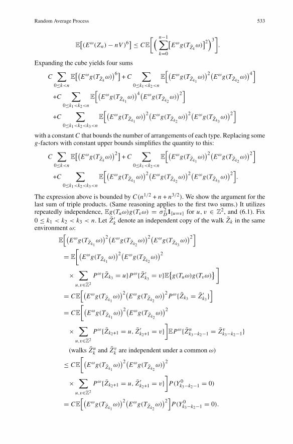
Random Average Process 533
E[(Eω(Zn) − nV )6] ≤ CE
[( n−1∑
k=0
[Eωg(TZk
ω)]2)3
]
.
Expanding the cube yields four sums
C∑
0≤k<n
E[(
Eωg(TZkω))6] + C
∑
0≤k1<k2<n
E
[(Eωg(TZk1
ω))2(
Eωg(TZk2ω))4]
+C∑
0≤k1<k2<n
E
[(Eωg(TZk1
ω))4(
Eωg(TZk2ω))2]
+C∑
0≤k1<k2<k3<n
E
[(Eωg(TZk1
ω))2(
Eωg(TZk2ω))2(
Eωg(TZk3ω))2]
with a constant C that bounds the number of arrangements of each type. Replacing someg-factors with constant upper bounds simplifies the quantity to this:
C∑
0≤k<n
E[(
Eωg(TZkω))2] + C
∑
0≤k1<k2<n
E
[(Eωg(TZk1
ω))2(
Eωg(TZk2ω))2]
+C∑
0≤k1<k2<k3<n
E
[(Eωg(TZk1
ω))2(
Eωg(TZk2ω))2(
Eωg(TZk3ω))2]
.
The expression above is bounded by C(n1/2 + n + n3/2). We show the argument for thelast sum of triple products. (Same reasoning applies to the first two sums.) It utilizesrepeatedly independence, Eg(Tuω)g(Tvω) = σ 2
D1{u=v} for u, v ∈ Z2, and (6.1). Fix
0 ≤ k1 < k2 < k3 < n. Let Z ′k denote an independent copy of the walk Zk in the same
environment ω:
E
[(Eωg(TZk1
ω))2(
Eωg(TZk2ω))2(
Eωg(TZk3ω))2]
= E
[(Eωg(TZk1
ω))2(
Eωg(TZk2ω))2
×∑
u,v∈Z2
Pω{Zk3 = u}Pω{Z ′k3
= v}E{g(Tuω)g(Tvω)}]
= CE
[(Eωg(TZk1
ω))2(
Eωg(TZk2ω))2
Pω{Zk3 = Z ′k3
}]
= CE
[(Eωg(TZk1
ω))2(
Eωg(TZk2ω))2
×∑
u,v∈Z2
Pω{Zk2+1 = u, Z ′k2+1 = v}
]
EPω{Z uk3−k2−1 = Zv
k3−k2−1}
(walks Z uk and Zv
k are independent under a common ω)
≤ CE
[(Eωg(TZk1
ω))2(
Eωg(TZk2ω))2
×∑
u,v∈Z2
Pω{Zk2+1 = u, Z ′k2+1 = v}
]
P(Y 0k3−k2−1 = 0)
= CE
[(Eωg(TZk1
ω))2(
Eωg(TZk2ω))2]
P(Y 0k3−k2−1 = 0).

534 M. Balázs, F. Rassoul-Agha, T. Seppäläinen
Now repeat the same step, and ultimately arrive at
∑
0≤k1<k2<k3<n
E
[(Eωg(TZk1
ω))2(
Eωg(TZk2ω))2(
Eωg(TZk3ω))2]
≤ C∑
0≤k1<k2<k3<n
P(Y 0k1
= 0)P(Y 0k2−k1−1 = 0)P(Y 0
k3−k2−1 = 0)
≤ C · Gn−1(0, 0)3 ≤ Cn3/2.
��By Theorem 8.8 in [12, Chap. 3],
E[(
an(t + h, r) − an(t, r))3(
an(t, r) − an(t − h, r))3 ] ≤ Ch3/2
is sufficient for tightness of the processes {an(t, r) : t ≥ 0}. The left-hand side above isbounded by
E[(
an(t + h, r) − an(t, r))6 ] + E
[(an(t, r) − an(t − h, r)
)6 ].
Note that if h < 1/(2n) then(an(t + h, r) − an(t, r)
)(an(t, r) − an(t − h, r)
) = 0 dueto the discrete time of the unscaled walks, while if h ≥ 1/(2n) then �n(t + h)�−�nt� ≤3nh. Putting these points together shows that tightness will follow from the next momentbound.
Lemma 6.2. There exists a constant 0 < C < ∞ such that, for all 0 ≤ m < n ∈ N,
E[({Eω(Z0,0
n ) − nV } − {Eω(Z0,0m ) − mV })6 ] ≤ C(n − m)3/2.
Proof. The claim reduces to Lemma 6.1 by restarting the walks at time m. ��Convergence of finite-dimensional distributions in Corollary 3.5 follows from Theo-
rem 3.4. The limiting process a(·)= lim an(·, r) is identified by its covariance Ea(s)a(t)=�q((s ∧ t, r), (s ∧ t, r)
). This completes the proof of Corollary 3.5.
7. Proofs for the Random Average Process
This section requires Theorem 3.2 from the space-time RWRE section.
7.1. Separation of effects. As the form of the limiting process in Theorem 2.1 suggests,we can separate the fluctuations that come from the initial configuration from those cre-ated by the dynamics. The quenched means of the RWRE represent the latter. We startwith the appropriate decomposition. Abbreviate
xn,r = x(n, r) = �n y� + �r√
n �.

Random Average Process 535
Recall that we are considering y ∈ R fixed, while (t, r) ∈ R+ ×R is variable and servesas the index for the process,
σ n�nt�(xn,r + �ntb�) − σ n0 (xn,r ) = Eω
[σ n
0 (X x(n,r)+�ntb�, �nt��nt� ) − σ n
0 (xn,r )]
= Eω
[
1{X x(n,r)+�ntb�, �nt�
�nt� >x(n,r)}
X x(n,r)+�ntb�, �nt��nt� ∑
i=x(n,r)+1
ηn0(i)
−1{X x(n,r)+�ntb�, �nt�
�nt� <x(n,r)}
x(n,r)∑
i=X x(n,r)+�ntb�, �nt��nt� +1
ηn0(i)
]
=∑
i>x(n,r)
Pω{
i ≤ X x(n,r)+�ntb�, �nt��nt�
}· ηn
0(i)
−∑
i≤x(n,r)
Pω{
i > X x(n,r)+�ntb�, �nt��nt�
}· ηn
0(i).
Recalling the means �(i/n) = Eηn0(i) we write this as
σ n�nt�(xn,r + �ntb�) − σ n0 (xn,r ) = Y n(t, r) + Hn(t, r), (7.1)
where
Y n(t, r) =∑
i∈Z
(ηn
0(i) − �(i/n))(
1{i > xn,r }Pω{
i ≤ X x(n,r)+�ntb�, �nt��nt�
}
− 1{i ≤ xn,r }Pω{i > X x(n,r)+�ntb�, �nt�
�nt�})
and
Hn(t, r) =∑
i∈Z
�(i/n)(
1{i > xn,r }Pω{i ≤ X x(n,r)+�ntb�, �nt�
�nt�}
− 1{i ≤ xn,r }Pω{i > X x(n,r)+�ntb�, �nt�
�nt�})
.
The plan of the proof of Theorem 2.1 is summarized in the next lemma. In the pagesthat follow we then show the finite-dimensional weak convergence n−1/4 Hn → H , andthe finite-dimensional weak convergence n−1/4Y n → Y for a fixed ω. This last statementis actually not proved quite in the strength just stated, but the spirit is correct. The distri-butional limit n−1/4Y n → Y comes from the centered initial increments ηn
0(i)−�(i/n),
while a homogenization effect takes place for the coefficients Pω{i ≤ X x(n,r)+�ntb�, �nt��nt� }
which converge to limiting deterministic Gaussian probabilities. Since the initial heightfunctions σ n
0 and the random environments ω that drive the dynamics are independent,we also get convergence n−1/4(Y n + Hn) → Y + H with independent terms Y and H .This is exactly the statement of Theorem 2.1.
Lemma 7.1. Let (�0,F0, P0) be a probability space on which are defined independentrandom variables η and ω with values in some abstract measurable spaces. The marginallaws are P for ω and P for η, and Pω = δω ⊗ P is the conditional probability distribu-tion of (ω, η), given ω. Let Hn(ω) and Yn(ω, η) be R
N -valued measurable functions of(ω, η). Make assumptions (i)–(ii) below.

536 M. Balázs, F. Rassoul-Agha, T. Seppäläinen
(i) There exists an RN -valued random vector H such that Hn(ω) converges weakly to H.
(ii) There exists an RN -valued random vector Y such that, for all θ ∈ R
N ,
Eω[eiθ ·Yn ] → E(eiθ ·Y) in P-probability as n → ∞.
Then Hn + Yn converges weakly to H + Y, where H and Y are independent.
Proof. Let θ, λ be arbitrary vectors in RN . Then
∣∣∣EEω
[eiλ·Hn+iθ ·Yn
]− E
[eiλ·H] E
[eiθ ·Y]
∣∣∣
≤∣∣∣E[eiλ·Hn
(Eωeiθ ·Yn − Eeiθ ·Y)]
∣∣∣ +∣∣∣(Eeiλ·Hn − Eeiλ·H) Eeiθ ·Y
∣∣∣
≤∣∣∣E[eiλ·Hn
(Eωeiθ ·Yn − Eeiθ ·Y)]
∣∣∣ +∣∣∣Eeiλ·Hn − Eeiλ·H
∣∣∣ .
By assumption (i), the second term above goes to 0. By assumption (ii), the integrandin the first term goes to 0 in P-probability. Therefore by bounded convergence the firstterm goes to 0 as n → ∞. ��
Turning to the work itself, we check first that Hn(t, r) can be replaced with a quenchedRWRE mean. Then the convergence Hn → H follows from the RWRE results.
Lemma 7.2. For any S, T < ∞ and for P-almost every ω,
limn→∞ sup
0≤t≤T−S≤r≤S
n−1/4∣∣∣Hn(t, r) − �(y) · Eω
(X x(n,r)+�ntb�, �nt�
�nt� − xn,r)∣∣∣ = 0.
Proof. Decompose Hn(t, r) = Hn1 (t, r) − Hn
2 (t, r), where
Hn1 (t, r) =
∑
i>x(n,r)
Pω{
i ≤ X x(n,r)+�ntb�, �nt��nt�
}· �(i/n),
Hn2 (t, r) =
∑
i≤x(n,r)
Pω{
i > X x(n,r)+�ntb�, �nt��nt�
}· �(i/n).
Working with Hn1 (t, r), we separate out the negligible error,
Hn1 (t, r) = �(y)
∑
i>x(n,r)
Pω{
i ≤ X x(n,r)+�ntb�, �nt��nt�
}
+∑
i>x(n,r)
Pω{
i ≤ X x(n,r)+�ntb�, �nt��nt�
}· [�(i/n) − �(y)
]
= �(y) · Eω[(
X x(n,r)+�ntb�, �nt��nt� − xn,r
)+]+ R1(t, r)
with
R1(t, r) =∞∑
m=1
Pω{
xn,r + m ≤ X x(n,r)+�ntb�, �nt��nt�
}·[�( xn,r
n+
m
n
)− �(y)
].

Random Average Process 537
Fix a small positive number δ < 12 , and use the boundedness of probabilities and the
function �:
|R1(t, r)| ≤�n1/2+δ�∑
m=1
∣∣∣�( xn,r
n+
m
n
)− �(y)
∣∣∣
+ C ·∞∑
m=�n1/2+δ�+1
Pω{
xn,r + m ≤ X x(n,r)+�ntb�, �nt��nt�
}. (7.2)
By the local Hölder-continuity of � with exponent γ > 12 , the first sum is o(n1/4) if
δ > 0 is small enough. Since X x(n,r)+�ntb�,�nt�0 = xn,r +�ntb� and by time �nt� the walk
has displaced by at most M�nt�, there are at most O(n) nonzero terms in the secondsum in (7.2). Consequently this sum is at most
Cn · Pω{
X x(n,r)+�ntb�, �nt��nt� − xn,r ≥ �n1/2+δ�
}.
By Lemma 4.3 the last line vanishes uniformly over t ∈ [0, T ] and r ∈ [−S, S] asn → ∞, for P-almost every ω. We have shown
limn→∞ sup
0≤t≤T−S≤r≤S
n−1/4∣∣∣Hn
1 (t, r) − �(y) · Eω[(
X x(n,r)+�ntb�, �nt��nt� − xn,r
)+ ]∣∣∣ = 0 P-a.s.
Similarly one shows
limn→∞ sup
0≤t≤T−S≤r≤S
n−1/4∣∣∣Hn
2 (t, r) − �(y) · Eω[(
X x(n,r)+�ntb�, �nt��nt� − xn,r
)− ]∣∣∣ = 0 P-a.s.
The conclusion follows from the combination of these two. ��For a fixed n and y, the process Eω
(X x(n,r)+�ntb�, �nt�
�nt� − xn,r)
has the same distribu-tion as the process yn(t, r) defined in (3.6). A combination of Lemma 7.2 and Theorem3.2 imply that the finite-dimensional distributions of the processes n−1/4 Hn convergeweakly, as n → ∞, to the finite-dimensional distributions of the mean-zero Gaussianprocess H with covariance
E H(s, q)H(t, r) = �(y)2�q((s, q), (t, r)). (7.3)
7.2. Finite-dimensional convergence of Y n. Next we turn to convergence of the finite-dimensional distributions of process Y n in (7.1). Recall that B(t) is standard Brownianmotion, and σ 2
a = E[(X0,01 − V )2] is the variance of the annealed walk. Recall the
definition
�0((s, q), (t, r)) =∫ ∞
q∨rP[σa B(s) > x − q]P[σa B(t) > x − r ] dx
−{
1{r>q}∫ r
qP[σa B(s) > x − q]P[σa B(t) ≤ x − r ] dx
+1{q>r}∫ q
rP[σa B(s) ≤ x − q]P[σa B(t) > x − r ] dx
}
+∫ q∧r
−∞P[σa B(s) ≤ x − q]P[σa B(t) ≤ x − r ] dx .

538 M. Balázs, F. Rassoul-Agha, T. Seppäläinen
Recall from (2.9) that v(y) is the variance of the increments around �n y�. Let {Y (t, r) :t ≥ 0, r ∈ R} be a real-valued mean-zero Gaussian process with covariance
EY (s, q)Y (t, r) = v(y)�0((s, q), (t, r)). (7.4)
Fix N and space-time points (t1, r1), . . . , (tN , rN ) ∈ R+ × R. Define vectors
Yn = n−1/4(Y n(t1, r1), . . . , Y n(tN , rN ))
and Y = (Y (t1, r1), . . . , Y (tN , rN )).
This section is devoted to the proof of the next proposition, after which we finish theproof of Theorem 2.1.
Proposition 7.1. For any vector θ = (θ1, . . . , θN ) ∈ RN , Eω(eiθ ·Yn
) → E(eiθ ·Y) inP-probability as n → ∞.
Proof. Let G be a centered Gaussian variable with variance
S = v(y)
N∑
k, l=1
θkθl�0((tk, rk), (tl , rl))
and so θ · Y is distributed like G. We will show that
Eω(eiθ ·Yn) → E(eiG) in P-probability. (7.5)
Recalling the definition of Y n(t, r), introduce some notation:
ζωn (i, t, r) = 1{i > xn,r }Pω
{i ≤ X x(n,r)+�ntb�, �nt�
�nt�}
− 1{i ≤ xn,r }Pω{i > X x(n,r)+�ntb�, �nt�
�nt�}
so that
Y n(t, r) =∑
i∈Z
(ηn
0(i) − �(i/n))ζω
n (i, t, r).
Then put
νωn (i) =
N∑
k=1
θk ζωn (i, tk, rk)
and
Un(i) = n−1/4 (ηn0(i) − �(i/n)
)νω
n (i).
Consequently
θ · Yn =∑
i∈Z
Un(i).
To separate out the relevant terms let δ > 0 be small and define
Wn =�n y�+�n1/2+δ�∑
i=�n y�−�n1/2+δ�Un(i).

Random Average Process 539
For fixed ω and n, under the measure Pω the variables {Un(i)} are constant multiples ofcentered increments ηn
0(i) − �(i/n) and hence independent and mean zero. Recall alsothat second moments of centered increments ηn
0(i) − �(i/n) are uniformly bounded.Thus the terms left out of Wn satisfy
Eω[(Wn − θ · Yn)2 ] ≤ Cn−1/2
∑
i :|i−�n y� | > n1/2+δ
νωn (i)2,
and we wish to show that this upper bound vanishes for P-almost every ω as n → ∞.Using the definition of νω
n (i), bounding the sum on the right reduces to bounding sumsof the two types
n−1/2∑
i :|i−�n y� | > n1/2+δ
1{i > x(n, rk)}(
Pω{i ≤ X x(n,rk )+�ntk b�, �ntk�
�ntk�})2
and
n−1/2∑
i :|i−�n y� | > n1/2+δ
1{i ≤ x(n, rk)}(
Pω{i > X x(n,rk )+�ntk b�, �ntk�
�ntk�})2
.
For large enough n the points x(n, rk) lie within 12 n1/2+δ of �n y�, and then the previous
sums are bounded by the sums
n−1/2∑
i ≥ x(n,rk )+(1/2)n1/2+δ
(Pω{i ≤ X x(n,rk )+�ntk b�, �ntk�
�ntk�})2
and
n−1/2∑
i ≤ x(n,rk )−(1/2)n1/2+δ
(Pω{i > X x(n,rk )+�ntk b�, �ntk�
�ntk�})2
.
These vanish for P-almost every ω as n → ∞ by Lemma 4.3, in a manner similar to thesecond sum in (7.2). Thus Eω
[(Wn − θ ·Yn)2
]→ 0 and our goal (7.5) has simplified to
Eω(eiWn ) → E(eiG) in P-probability. (7.6)
We use the Lindeberg-Feller theorem to formulate conditions for a central limittheorem for Wn under a fixed ω. For Lindeberg-Feller we need to check two conditions:
(LF-i) Sn(ω) ≡�n y�+�n1/2+δ�∑
i=�n y�−�n1/2+δ�Eω[Un(i)
2]
−→n→∞ S,
(LF-ii)�n y�+�n1/2+δ�∑
i=�n y�−�n1/2+δ�Eω[Un(i)2 · 1{|Un(i)|>ε}
]−→n→∞ 0 for all ε > 0.
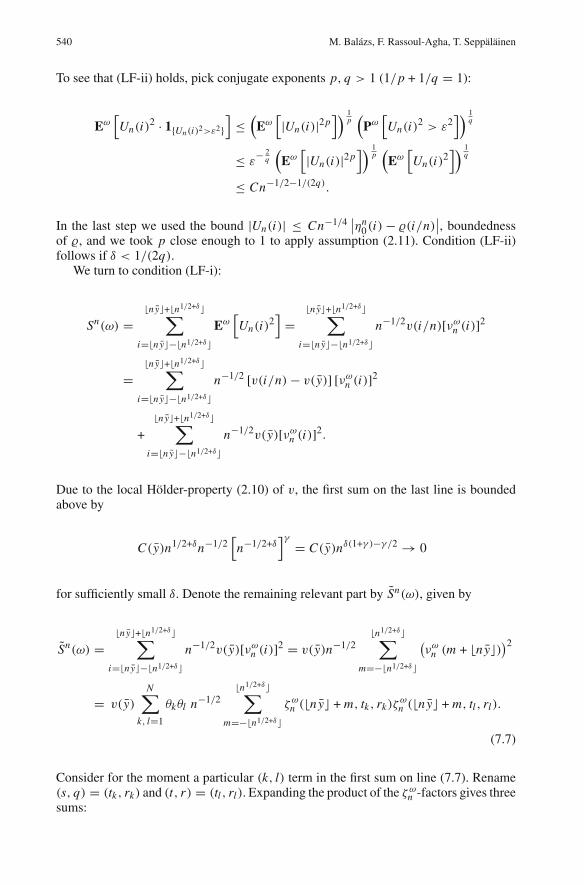
540 M. Balázs, F. Rassoul-Agha, T. Seppäläinen
To see that (LF-ii) holds, pick conjugate exponents p, q > 1 (1/p + 1/q = 1):
Eω[Un(i)2 · 1{Un(i)2>ε2}
]≤(
Eω[|Un(i)|2p
]) 1p(
Pω[Un(i)
2 > ε2]) 1
q
≤ ε− 2
q
(Eω[|Un(i)|2p
]) 1p(
Eω[Un(i)2
]) 1q
≤ Cn−1/2−1/(2q).
In the last step we used the bound |Un(i)| ≤ Cn−1/4∣∣ηn
0(i) − �(i/n)∣∣, boundedness
of �, and we took p close enough to 1 to apply assumption (2.11). Condition (LF-ii)follows if δ < 1/(2q).
We turn to condition (LF-i):
Sn(ω) =�n y�+�n1/2+δ�∑
i=�n y�−�n1/2+δ�Eω[Un(i)2
]=
�n y�+�n1/2+δ�∑
i=�n y�−�n1/2+δ�n−1/2v(i/n)[νω
n (i)]2
=�n y�+�n1/2+δ�∑
i=�n y�−�n1/2+δ�n−1/2 [v(i/n) − v(y)] [νω
n (i)]2
+�n y�+�n1/2+δ�∑
i=�n y�−�n1/2+δ�n−1/2v(y)[νω
n (i)]2.
Due to the local Hölder-property (2.10) of v, the first sum on the last line is boundedabove by
C(y)n1/2+δn−1/2[n−1/2+δ
]γ = C(y)nδ(1+γ )−γ /2 → 0
for sufficiently small δ. Denote the remaining relevant part by Sn(ω), given by
Sn(ω) =�n y�+�n1/2+δ�∑
i=�n y�−�n1/2+δ�n−1/2v(y)[νω
n (i)]2 = v(y)n−1/2�n1/2+δ�∑
m=−�n1/2+δ�
(νω
n (m + �n y�))2
= v(y)
N∑
k, l=1
θkθl n−1/2�n1/2+δ�∑
m=−�n1/2+δ�ζω
n (�n y� + m, tk, rk)ζωn (�n y� + m, tl , rl).
(7.7)
Consider for the moment a particular (k, l) term in the first sum on line (7.7). Rename(s, q) = (tk, rk) and (t, r) = (tl , rl). Expanding the product of the ζω
n -factors gives threesums:

Random Average Process 541
n−1/2�n1/2+δ�∑
m=−�n1/2+δ�ζω
n (�n y� + m, s, q)ζωn (�n y� + m, t, r)
= n−1/2�n1/2+δ�∑
m=−�n1/2+δ�1{m>�q
√n �}1{m>�r
√n �} Pω
(X x(n,q)+�nsb�, �ns�
�ns� ≥ �n y� + m)
×Pω(X x(n,r)+�ntb�, �nt�
�nt� ≥ �n y� + m)
(7.8)
− n−1/2�n1/2+δ�∑
m=−�n1/2+δ�
{
1{m>�q√
n �}1{m≤�r√
n �} Pω(X x(n,q)+�nsb�, �ns�
�ns� ≥ �n y� + m)
×Pω(X x(n,r)+�ntb�, �nt�
�nt� < �n y� + m)
+ 1{m≤�q√
n �}1{m>�r√
n �} Pω(X x(n,q)+�nsb�, �ns�
�ns� < �n y� + m)
×Pω(X x(n,r)+�ntb�, �nt�
�nt� ≥ �n y� + m)}
(7.9)
+ n−1/2�n1/2+δ�∑
m=−�n1/2+δ�1{m≤�q
√n �}1{m≤�r
√n �} Pω
(X x(n,q)+�nsb�, �ns�
�ns� < �n y� + m)
×Pω(X x(n,r)+�ntb�, �nt�
�nt� < �n y� + m). (7.10)
Each of these three sums (7.8)–(7.10) converges to a corresponding integral in P-prob-ability, due to the quenched CLT Theorem 3.1. To see the correct limit, just note that
Pω(X x(n,r)+�ntb�, �nt�
�nt� < �n y� + m)
= Pω(X x(n,r)+�ntb�, �nt�
�nt� − X x(n,r)+�ntb�,�nt�0 < −�ntb� + m − �r
√n � ),
and recall that −b = V is the average speed of the walks. We give technical details ofthe argument for the first sum in the next lemma.
Lemma 7.3. As n → ∞, the sum in (7.8) converges in P-probability to
∫ ∞
q∨rP[σa B(s) > x − q]P[σa B(t) > x − r ] dx .
Proof of Lemma 7.3. With
f ωn (x) = Pω
(X x(n,q)+�nsb�, �ns�
�ns� ≥ �n y� + �x√
n�)
×Pω(X x(n,r)+�ntb�, �nt�
�nt� ≥ �n y� + �x√
n�)
and
I ωn =
∫ nδ
q∨rf ωn (x)dx,

542 M. Balázs, F. Rassoul-Agha, T. Seppäläinen
the sum in (7.8) equals I ωn + O(n−1/2). By the quenched invariance principle Theorem
3.1, for any fixed x , f ωn (x) converges in P-probability to
f (x) = P[σa B(s) ≥ x − q]P[σa B(t) ≥ x − r ].
We cannot claim this convergence P-almost surely because the walks X x(n,r)+�ntb�, �nt��nt�
change as n changes. But by a textbook characterization of convergence in probability,for a fixed x each subsequence n( j) has a further subsequence n( j�) such that
P
[ω : f ω
n( j�)(x) −→
�→∞ f (x)]
= 1.
By the diagonal trick, one can find one subsequence for all x ∈ Q and thus
∀{n( j)}, ∃{ j�} : P
[ω : ∀x ∈ Q : f ω
n( j�)(x) → f (x)
]= 1.
Since f ωn and f are nonnegative and nonincreasing, and f is continuous and decreases
to 0, the convergence works for all x and is uniform on [q ∨ r,∞). That is,
∀{n( j)}, ∃{ j�} : P
[ω :
∥∥∥ f ω
n( j�)− f
∥∥∥
L∞[q∨r,∞)→ 0
]= 1.
It remains to make the step to the convergence of the integral I ωn to
∫∞q∨r f (x) dx .
Define now
Jωn (A) =
∫ A
q∨rf ωn (x)dx .
Then, for any A < ∞,
∀{n( j)}, ∃{ j�} : P
[ω : Jω
n( j�)(A) →
∫ A
q∨rf (x)dx
]= 1.
In other words, Jωn (A) converges to
∫ Aq∨r f (x)dx in P-probability. Thus, for each 0 <
A < ∞, there is an integer m(A) such that for all n ≥ m(A),
P
[
ω :∣∣∣Jω
n (A) −∫ A
q∨rf (x)dx
∣∣∣ > A−1
]
< A−1.
Pick An ↗ ∞ such that m(An) ≤ n. Under the annealed measure P , X0,0n is a homo-
geneous mean zero random walk with variance O(n). Consequently
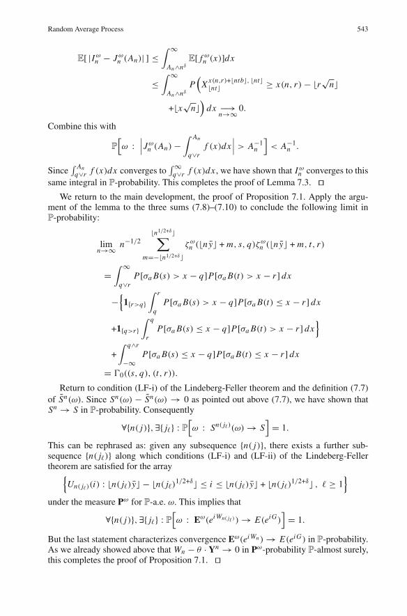
Random Average Process 543
E[ |I ωn − Jω
n (An)| ] ≤∫ ∞
An∧nδ
E[ f ωn (x)]dx
≤∫ ∞
An∧nδ
P(
X x(n,r)+�ntb�, �nt��nt� ≥ x(n, r) − �r
√n�
+�x√
n�)
dx −→n→∞ 0.
Combine this with
P
[ω :
∣∣∣Jω
n (An) −∫ An
q∨rf (x)dx
∣∣∣ > A−1
n
]< A−1
n .
Since∫ An
q∨r f (x)dx converges to∫∞
q∨r f (x)dx , we have shown that I ωn converges to this
same integral in P-probability. This completes the proof of Lemma 7.3. ��We return to the main development, the proof of Proposition 7.1. Apply the argu-
ment of the lemma to the three sums (7.8)–(7.10) to conclude the following limit inP-probability:
limn→∞ n−1/2
�n1/2+δ�∑
m=−�n1/2+δ�ζω
n (�n y� + m, s, q)ζωn (�n y� + m, t, r)
=∫ ∞
q∨rP[σa B(s) > x − q]P[σa B(t) > x − r ] dx
−{
1{r>q}∫ r
qP[σa B(s) > x − q]P[σa B(t) ≤ x − r ] dx
+1{q>r}∫ q
rP[σa B(s) ≤ x − q]P[σa B(t) > x − r ] dx
}
+∫ q∧r
−∞P[σa B(s) ≤ x − q]P[σa B(t) ≤ x − r ] dx
= �0((s, q), (t, r)).
Return to condition (LF-i) of the Lindeberg-Feller theorem and the definition (7.7)of Sn(ω). Since Sn(ω) − Sn(ω) → 0 as pointed out above (7.7), we have shown thatSn → S in P-probability. Consequently
∀{n( j)}, ∃{ j�} : P
[ω : Sn( j�)(ω) → S
]= 1.
This can be rephrased as: given any subsequence {n( j)}, there exists a further sub-sequence {n( j�)} along which conditions (LF-i) and (LF-ii) of the Lindeberg-Fellertheorem are satisfied for the array{
Un( j�)(i) : �n( j�)y� − �n( j�)1/2+δ� ≤ i ≤ �n( j�)y� + �n( j�)
1/2+δ� , � ≥ 1}
under the measure Pω for P-a.e. ω. This implies that
∀{n( j)}, ∃{ j�} : P
[ω : Eω(eiWn( j�) ) → E(eiG)
]= 1.
But the last statement characterizes convergence Eω(eiWn ) → E(eiG) in P-probability.As we already showed above that Wn − θ · Yn → 0 in Pω-probability P-almost surely,this completes the proof of Proposition 7.1. ��

544 M. Balázs, F. Rassoul-Agha, T. Seppäläinen
7.3. Proofs of Theorem 2.1 and Proposition 2.2.
Proof of Theorem 2.1. The decomposition (7.1) gives zn = n−1/4(Y n + Hn). The para-graph that follows Lemma 7.2 and Proposition 7.1 verify the hypotheses of Lemma 7.1for Hn and Y n . Thus we have the limit zn → z ≡ Y + H in the sense of convergenceof finite-dimensional distributions. Since Y and H are mutually independent mean-zeroGaussian processes, their covariances in (7.3) and (7.4) can be added to give (2.18). ��Proof of Proposition 2.2. The value (2.23) for β can be computed from (2.8), or fromthe probabilistic characterization (4.4) of β via Example 4.1. If we let u denote a randomvariable distributed like u0(0,−1), then we get
β = Eu − E(u2)
Eu − (Eu)2 and κ = E(u2) − (Eu)2
Eu − E(u2).
With obvious notational simplifications, the evolution step (2.22) can be rewritten as
η′(k) − ρ = (1 − uk)(η(k) − ρ) + uk−1(η(k − 1) − ρ) + (uk−1 − uk)ρ.
Square both sides, take expectations, use the independence of all variables {η(k −1), η(k), uk, uk−1} on the right, and use the requirement that η′(k) have the same variancev as η(k) and η(k − 1). The result is the identity
v = v(1 − 2Eu + 2E(u2)) + 2ρ2(E(u2) − (Eu)2)
from which follows v = κρ2. The rest of part (b) is a straightforward specialization of(2.18). ��
Acknowledgements. The authors thank P. Ferrari and L. R. Fontes for comments on article [14] and J. Swansonfor helpful discussions.
References
1. Aldous, D., Diaconis, P.: Hammersley’s interacting particle process and longest increasing subsequences.Probab. Theory Related Fields 103(2), 199–213 (1995)
2. Aldous, D., Diaconis, P.: Longest increasing subsequences: from patience sorting to the Baik-Deift-Jo-hansson theorem. Bull. Amer. Math. Soc. (N.S.) 36(4), 413–432 (1999)
3. Baik, J., Deift, P., Johansson, K.: On the distribution of the length of the longest increasing subsequenceof random permutations. J. Amer. Math. Soc. 12(4), 1119–1178 (1999)
4. Balázs, M.: Growth fluctuations in a class of deposition models. Ann. Inst. H. Poincaré Probab. Statist.39(4), 639–685 (2003)
5. Bernabei, M.S.: Anomalous behaviour for the random corrections to the cumulants of random walks influctuating random media. Probab. Theory Related Fields 119(3), 410–432 (2001)
6. Boldrighini, C., Pellegrinotti, A.: T −1/4-noise for random walks in dynamic environment on Z. Mosc.Math. J. 1(3), 365–380 470–471 (2001)
7. Burkholder, D.L.: Distribution function inequalities for martingales. Ann. Probab. 1, 19–42 (1973)8. Chung, K.L.: Markov chains with stationary transition probabilities. In: Die Grundlehren der mathemat-
ischen Wissenschaften, Band 104. New York: Springer-Verlag Second edition, 19679. De Masi, A., Presutti, E.: Mathematical methods for hydrodynamic limits, Volume 1501 of Lecture Notes
in Mathematics. Berlin: Springer-Verlag, 199110. Deift, P.: Integrable systems and combinatorial theory. Notices Amer. Math. Soc. 47(6), 631–640 (2000)11. Durrett, R.: Probability: theory and examples. Duxbury Advanced Series. Belmont, CA: Brooks/Cole–
Thomson, Third edition, 200412. Ethier, S.N., Kurtz, T.G.: Markov processes. Wiley Series in Probability and Mathematical Statistics:
Probability and Mathematical Statistics. New York: John Wiley & Sons Inc., 1986
Random Average Process 545
13. Ferrari, P.A., Fontes, L.R.G.: Current fluctuations for the asymmetric simple exclusion process. Ann.Probab. 22(2), 820–832 (1994)
14. Ferrari, P.A., Fontes, L.R.G.: Fluctuations of a surface submitted to a random average process. Electron.J. Probab. 3, no. 6, 34 pp., (1998) (electronic)
15. Ferrari, P.L., Spohn, H: Scaling Limit for the Space-Time Covariance of the Stationary Totally Asym-metric Simple Exclusion Process. Commum. Math. Phys. (2006) (in press)
16. Gravner, J., Tracy, C.A., Widom, H.: Limit theorems for height fluctuations in a class of discrete spaceand time growth models. J. Stat. Phys. 102(5–6), 1085–1132 (2001)
17. Groeneboom, P.: Hydrodynamical methods for analyzing longest increasing subsequences. J. Comput.Appl. Math. 142(1), 83–105 (2002)
18. Hammersley, J.M.: A few seedlings of research. In: Proceedings of the Sixth Berkeley Symposium onMathematical Statistics and Probability (Univ. California, Berkeley, Calif., 1970/1971), Vol. I: Theory ofstatistics, Berkeley, Univ. California Press, 1972, pp. 345–394
19. Johansson, K.: Shape fluctuations and random matrices. Commun. Math. Phys. 209(2), 437–476 (2000)20. Johansson, K.: Discrete orthogonal polynomial ensembles and the Plancherel measure. Ann. Math. (2)
153(1), 259–296 (2001)21. Kipnis, C., Landim, C.: Scaling limits of interacting particle systems. Volume 320 of Grundlehren der
Mathematischen Wissenschaften [Fundamental Principles of Mathematical Sciences], Berlin: Springer-Verlag 1999
22. Liggett, T.M.: Interacting particle systems. Volume 276 of Grundlehren der Mathematischen Wissens-chaften [Fundamental Principles of Mathematical Sciences], New York: Springer-Verlag 1985
23. Liggett, T.M.: Stochastic interacting systems: contact, voter and exclusion processes. Volume 324 ofGrundlehren der Mathematischen Wissenschaften [Fundamental Principles f Mathematical Sciences],Berlin: Springer-Verlag, 1999
24. Rassoul-Agha, F., Seppäläinen, T.: An almost sure invariance principle for random walks in a space-timerandom environment. Probab. The. Rel. Fields 133, no. 3, 299–314 (2005)
25. Rezakhanlou, F.: A central limit theorem for the asymmetric simple exclusion process. Ann. Inst. H.Poincaré Probab. Statist. 38(4), 437–464 (2002)
26. Seppäläinen, T.: A microscopic model for the Burgers equation and longest increasing subsequences.Electron. J. Probab. 1, no. 5, approx. 51 pp., (1996) (electronic)
27. Seppäläinen, T.: Exact limiting shape for a simplified model of first-passage percolation on the plane.Ann. Probab. 26(3), 1232–1250 (1998)
28. Seppäläinen, T.: Large deviations for increasing sequences on the plane. Probab. Th. Rel. Fields 112(2),221–244 (1998)
29. Seppäläinen, T.: Diffusive fluctuations for one-dimensional totally asymmetric interacting random dynam-ics. Commun. Math. Phys. 229(1), 141–182 (2002)
30. Seppäläinen, T.: Second-order fluctuations and current across characteristic for a one-dimensional growthmodel of independent random walks. Ann. Probab. 33(2), 759–797 (2005)
31. Spitzer, F.: Principles of random walk. New York: Springer-Verlag, 197632. Spohn, H.: Large scale dynamics of interacting particles. Berlin: Springer-Verlag 199133. Varadhan, S.R.S.: Lectures on hydrodynamic scaling. In Hydrodynamic limits and related topics (Toronto,
ON, 1998), Volume 27 of Fields Inst. Commun., Providence, RI: Amer. Math. Soc., 2000, pp. 3–4034. Walsh, J.B.: An introduction to stochastic partial differential equations. In: École d’été de probabilités de
Saint-Flour, XIV—1984, Volume 1180 of Lecture Notes in Math., Berlin: Springer, 1986, pp. 265–439
Communicated by H. Spohn