The Randomized Condorcet Voting System

Le Nguyen HoangMIT, lenhoang@mit.edu

March 24, 2017

Abstract

In this paper, we study the strategy-proofness properties of the randomized Condorcet voting system(RCVS). Discovered at several occasions independently, the RCVS is arguably the natural extensionof the Condorcet method to cases where a deterministic Condorcet winner does not exists. Indeed, itselects the always-existing and essentially unique Condorcet winner of lotteries over alternatives. Ourmain result is that, in a certain class of voting systems based on pairwise comparisons of alternatives,the RCVS is the only one to be Condorcet-proof. By Condorcet-proof, we mean that, when a Condorcetwinner exists, it must be selected and no voter has incentives to misreport his preferences. We also provetwo theorems about group-strategy-proofness. On one hand, we prove that there is no group-strategy-proof voting system that always selects existing Condorcet winners. On the other hand, we prove that,when preferences have a one-dimensional structure, the RCVS is group-strategy-proof.Keywords: Social choice Condorcet winner Strategy-proofness

1 Introduction

Social choice theory consists in choosing an alternative for a group of people whose individual preferencesmay greatly differ from one another. One of the first mathematicians to address this question was Condorcet(1785). Condorcet argued that an alternative that is preferred to any other by the majority should alwaysbe selected. Such an alternative is now known as a Condorcet winner. Unfortunately, Condorcet went onproving that a Condorcet winner does not necessarily exist, as he provided an example where the majorityprefers x to y, y to z and z to x. This example is now known as a Condorcet paradox. It has been the essenceof several impossibility theorems since. Namely, first, Arrow (1951) famously derived the impossibility of a”fair” aggregation of the preferences of the individuals into a preference of the group. Second, Gibbard (1973)and Satterthwaite (1975) proved that there is no strategy-proof, anonymous neutral and deterministic votingsystem. A similar result has been proved by Campbell and Kelly (1998) about the impossibility of combiningthe Condorcet principle with strategy-proofness for deterministic social choice rules that select one or twoalternatives. Third, Gibbard (1977, 1978) proved that random dictatorship was the only strategy-proof,anonymous, neutral and unanimous voting system, assuming voters’ preferences satisfy the Von Neumannand Morgenstern (1944) axioms.

Nevertheless, a natural extension of the concept of Condorcet winner to lotteries has been introducedand widely studied by Kreweras (1965), Fishburn (1984), Felsenthal and Machover (1992), Laslier (1997),Laslier (2000), Brandl et al. (2016), and relies on a remarkable existence and near-uniqueness theorem provedindependently by Fisher and Ryan (1992) and Laffond et al. (1993). Namely, it was proved that, providedthere is no tie between any two alternatives, and given a specific but natural extension of majority preferencesover candidates to preferences over lotteries, there always is a unique lottery that the majority likes at leastas much as any other lottery. We call such a lottery the Condorcet winner of lotteries, or the randomizedCondorcet winner. Naturally, it is this randomized Condorcet winner that we propose to select through therandomized Condorcet voting system (RCVS)1. The compelling naturalness of the RCVS has been further

1This voting system has been given different names in previous papers. These names include ”game-theory method” in

1

supported by Brandl et al. (2016) who characterized it as the only voting system satisfying three fairlynatural properties. What is perhaps most exciting is the recent implementation of the RCVS on the websitehttps://pnyx.dss.in.tum.de. In Section 2, we quickly redefine the RCVS and stress its naturalness.

In addition to this naturalness, the RCVS has been proved to possess appealing Pareto-efficiency prop-erties2. Indeed, Aziz et al. (2013) proved that random dictatorship and RCVS are two extreme points ofa tradeoff between Pareto-efficiency and strategy-proofness. Loosely, random dictatorship is, in some senserelated to the class of preferences considered3, more strategy-proof but less Pareto-efficient. Moreover, Azizet al. (2013, 2014) prove that, to a large extent, strategy-proofness and Pareto-efficiency are incompatible,which suggests that the RCVS can hardly be improved upon with respect to such considerations.

Unfortunately, the theorem by Gibbard (1977) implies that the RCVS is not strategy-proof for vonNeumann - Morgenstern preferences. The proof of this, along with many similar results, relies on theconcept of first-order stochastic dominance, which allows to capture the whole diversity of von Neumann- Morgenstern preferences. In particular, the harshness of Gibbard (1977)’s result is precisely due to howconstraining first-order stochastic dominance is. Thus, if we relax this condition, we may be able to provethe (thus weaker) strategy-proofness of some voting systems that are not random dictatorships. This is whathas been proposed by Bogomolnaia and Moulin (2001) and Balbuzanov (2016), who respectively introducedordinal efficiency and convex undomination. In this paper, we shall take another path, by studying a verydistinct (but still fairly natural) class of preferences based on pairwise comparisons of drawn alternatives,which was previously introduced by Fishburn (1982) and Aziz et al. (2015).

The main contribution of this paper is to show that, for this class of pairwise comparison preferences, theRCVS possesses enviable strategy-proofness properties. We prove that the RCVS is Condorcet-proof, in thesense that, when a Condorcet winner exists, the RCVS selects it and no voter has incentives to misreporthis preferences. We shall also show that, in a certain class of voting systems based on pairwise comparisonsof alternatives, the RCVS is the only one that is Condorcet-proof. These properties are formally stated andderived in Section 3. We shall argue that they are strong indications that the RCVS has key properties thatshould favor its use over other voting systems.

Next, in Section 4, we study the group strategy-proofness of voting systems. We start with an impossi-bility result that asserts that no voting system that selects Condorcet winners is group strategy-proof. Nextand finally, we restrict ourselves to the cases where alternatives range on a one-dimensional axis, which ismathematically described by two models known as single-peakedness and single-crossing. It is well-knownthat, under these models, Condorcet winners are guaranteed to exist (Black (1958); Roberts (1977); Roth-stein (1990, 1991); Gans and Smart (1996)). While the median social rule introduced by Moulin (1980)and generalized by Saporiti (2009) guarantees strategy-proofness for one-dimensional preferences, it requiresto explicitly and officially locate alternatives on a one-dimensional line, and to forbid voters’ ballots to beinconsistent with the assumed corresponding one-dimensional structure of preferences. In many cases, likein politics, this may not be acceptable. However, Penn et al. (2011) proved that, when preferences aresingle-peaked but ballots are not constrained to be single-peaked, a deterministic group-strategy-proof vot-ing system must be dictatorial. We shall prove that, under single-peakedness or single-crossing preferences,the RCVS is group-strategy-proof.

Finally, Section 5 concludes by emphatically recommending the use of the RCVS in practice.

Felsenthal and Machover (1992) which is not to be confused with the slightly different game-theory method by Rivest and Shen(2010), ”symmetric two-party competition game equilibrium” in Laslier (2000); Myerson (1996), ”maximal lottery” in Fishburn(1984); Aziz et al. (2013); Brandl et al. (2016) and ”Fishburn’s rule” on https://pnyx.dss.in.tum.de. Note that some of thesepapers also study variants where the margin by which an alternative x is preferred to y is taken into account (whereas, here,only the fact that is the majority prefers x matters). Finally, it should be added that the (support of the) RCVS has also beenstudied under the names ”bipartisan set” and ”essential set”. We believe, however, that our terminology yields greater insightinto the nature of this lottery.

2A voting system is Pareto-efficiency if there is no lottery x such that everyone likes x at least as much as the selected lottery,and someone strictly prefers x to the selected lottery.

3There are several possible ways to extend preferences over alternatives to preferences over lotteries, each leading to its ownconcepts of strategy-proofness and Pareto-efficiency.

2

2 The Randomized Condorcet Voting System

In this section, we briefly reintroduce the RCVS, which was repeatedly discovered in the literature. Weconsider a finite set X of alternatives. A preference θ ∈ O is an order4 over X. For simplicity, we shallrestrict our analysis to total order preferences, but there is no difficulty in generalizing our results to partialorders. We denote θ : x � y the fact that a voter with preference θ prefers alternative x to y. The anonymouspreferences of a population of voters can then be represented as a probability distribution θ ∈ ∆(O) overpreferences. Note that this representation of the preferences of a population does not discriminate certaindistinct settings, e.g. a population and two copies of this population. However, it has the advantageof modeling as well situations where different voters have different weights, e.g. in a company board ofdirectors. Now, we say that the majority Mθ prefers x to y if more people prefer x to y, i.e.

Mθ : x� y4⇐⇒ Pθ∼θ [θ : x � y] > Pθ∼θ [θ : x ≺ y] ,

where Pθ∼θ[·] is the probability of an event ”·” regarding a random voter θ drawn from the population θ.For convenience of notation, we use probability notations for quantities often rather regarded as frequencies.The line above can equivalently be read as the probability that a random voter prefers x to y is greater thanthe probability that he prefers y to x, or as the fraction of voters who prefer x to y being greater than thefraction of voters who prefer y to x.

We shall use the notation ”�” instead of ”�” when the right-hand inequality features the greater-or-equal sign ”≥”.

Example 1. Consider X = {x, y, z}, and θ ∈ ∆(O) defined by:

Pθ∼θ [θ : x � y � z] = 27/100,

Pθ∼θ [θ : z � x � y] = 31/100,

Pθ∼θ [θ : y � x � z] = 42/100.

We then have Mθ : x� y � z � x, which proves that the majority preference Mθ is not transitive and thatthere is no Condorcet winner. This is the infamous Condorcet paradox.

Given the limitations of deterministic voting systems proved by Gibbard (1973), Satterthwaite (1975)and Penn et al. (2011), we turn our attention to randomized voting systems, which have been gaininginterests in recent years (see, e.g. Ehlers et al. (2002); Bogomolnaia et al. (2005); Chatterji et al. (2014)).Instead of selecting an alternative, a randomized voting system selects a lottery x ∈ ∆(X), that is, aprobability distribution over alternatives. A crucial difficulty posed by the introduction of randomness insocial choice theory is the extension of preferences over deterministic alternatives to preferences over lotteries.To introduce and justify the randomized Condorcet voting system, it turns out to be sufficient to extend themajority preferences. We do this as follows. We say that the majority Mθ prefers a lottery x to a lotteryy, if the majority more often prefers the alternative drawn by x to the one drawn by y, than the other wayaround, i.e.

Mθ : x� y4⇐⇒ Px∼x,y∼y

[Mθ : x� y

]> Px∼x,y∼y

[Mθ : x� y

],

where, as earlier, the notation x ∼ x means that we are drawing x from the probability distribution x. Thisextension of majority preferences to lotteries shares strong similarities with the SSB preferences axiomatizedby Fishburn (1982), and even more with the pairwise comparison preferences studied by Aziz et al. (2014).We stress, however, that the majority preference Mθ need not be transitive over deterministic alternatives,which is evidently the essence of the Condorcet paradox. Nevertheless, we argue that this extension of

4An order is a binary relation that satisfies the following properties, for all x, y, z ∈ X:

• Antisymmetry: if θ : x � y and θ : y � x, then x = y.

• Transitivity: if θ : x � y and θ : y � z, then θ : x � z.If, in addition, the order satisfies totality, i.e. θ : x � y or θ : y � x, then we say that the order is total.

3

majority preferences over alternatives to majority preferences over lotteries is fairly natural, especially giventhat we assume to only have access to ordinal preferences of the voters.

The definition of majority preferences over lotteries can also be stated in terms of an inequality withmatrices. First, for any preferences θ of the people, let us define the referendum matrix R(θ) ∈ RX×X by

Rxy(θ) , Pθ∼θ [θ : x � y]− Pθ∼θ [θ : y � x] .

Intuitively, Rxy(θ) counts the relative proportion of voters that prefer x over y, and thus, the hypotheticalresult of a referendum opposing x to y.

Now, let us define A(Mθ) ∈ RX×X the skew-symmetric matrix that only remembers the signs of theentries of the referendum matrix. In other words, A(Mθ) is defined by

Axy(Mθ) =

+1, Mθ : x� y,−1, Mθ : x� y,0, otherwise.

Moreover, we can represent any lottery x by a vector p(x) ∈ RX defined by px(x) = Py∼x[x = y]. Then,

Mθ : x� y ⇐⇒ p(x)TA(Mθ)p(y) > 0,

Like earlier, we shall use the symbol ”�” when the right-hand side inequality features the greater-or-equalsign.

Remark 1. The definition of the majority preferences Mθ over lotteries is not to be confused with the factthat a random voter will more likely prefer x to y, nor with the fact that a random voter will more likelyprefer a random alternative drawn from x to one drawn from y.

Example 2. Let us reconsider Example 1. Recall that Mθ : x � y � z � x. Consider the lottery p thatassigns probability 2/3 to x and 1/3 to y, which we shall compare to z (or, equivalently, the lottery δz whichassigns probability 1 to z). Then, Pp∼p[Mθ : p � z] = Pp∼p[p = y] = 1/3, while Pp∼p[Mθ : z � p] =Pp∼p[p = x] = 2/3. In other words, two out of three times, the majority will prefer the alternative z to theone drawn by p, while only one third of the times it will prefer the alternative drawn by p to z. Therefore,the majority prefers z to p, i.e. Mθ : z � p.

Finally, we can generalize the concept of Condorcet winners of alternatives to Condorcet winners oflotteries. We say that a lottery x is a randomized Condorcet winner if there is no other lottery that themajority prefers, i.e. such that

∀y ∈ ∆(X), Mθ : x� y.

This definition of the majority preferences over lotteries then allows to circumvent the Condorcet paradoxin a very natural way, which relies on the following restatement of a well-known theorem.

Theorem 1 (Fisher and Ryan (1992); Felsenthal and Machover (1992); Laffond et al. (1993)). There alwaysexists a randomized Condorcet winner. Plus, if there is no tie between any two alternatives, the randomizedCondorcet winner is unique.

On one hand, the proofs of this theorem are not very constructive nor insightful. For instance, theexistence is derived from the minimax theorem by Von Neumann (1928) or the Nash (1951) theorem. Onthe other hand, though, the randomized Condorcet winner can be efficiently computed. Indeed, the set ofrandomized Condorcet winners is actually a polytope, whose variables are the probabilities of selecting thedifferent alternatives, and whose constraints assert that the majority must like the randomized Condorcetwinners at least as much as any deterministic alternative. Thus, a randomized Condorcet winner can becomputed by solving a basic LP with O(|X|) variables and constraints. Naturally, it is this essentially uniquerandomized Condorcet winner that we propose to select.

4

Definition 1. The randomized Condorcet voting system (RCVS) C : ∆(O)→ ∆(X) selects the randomizedCondorcet winner C (θ) of the majority preferences Mθ.5.

Note that any deterministic Condorcet winner is a randomized Condorcet winner. Therefore, by theuniqueness property, if a deterministic Condorcet winner exists, then the RCVS selects it deterministically.In any case, by construction, the RCVS has the following characteristic property:

∀x ∈ ∆(X), Mθ : C (θ)� x,

that is, the majority always prefers the randomized Condorcet winner at least as much as any lottery. Fromthis property, it is immediate that the RCVS satisfies independence of irrelevant alternatives, in the sensethat if an alternative is not in the support of C (θ), then removing it from the set of alternatives (which onlyimplies reducing the set ∆(X)) does not affect the value of lottery C (θ).

Example 3. We reconsider Example 1. Recall that Mθ : x� y � z � x, so that there was no deterministicCondorcet winner. In particular, note that Mθ : c� p if and only if (c, p) ∈ {(x, y), (y, z), (z, x)}. Here, the

randomized Condorcet winner C (θ) is the uniform distribution over X. Indeed, let p the lottery that assignsprobabilities px, py and pz to alternatives x, y and z. Then,

Pc∼C (θ),p∼p[Mθ : c� p

]= P [(c, p) ∈ {(x, y), (y, z), (z, x)}]

= P [(c, p) = (x, y)] + P[(c, p) = (y, z)] + P[(c, p) = (z, x)]

=py3

+pz3

+px3

= P [(c, p) = (z, y)] + P[(c, p) = (x, z)] + P[(c, p) = (y, x)]

= P [(c, p) ∈ {(z, y), (x, z), (y, x)}]= P

[Mθ : c� p

],

where all the probabilities are obtained by drawing c from C (θ) and p from p. This proves that the majorityMθ likes C (θ) just as much as p. In particular, we have Mθ : C (θ) � p, for any lottery p. This is thecharacteristic property of the RCVS.

Example 4. As another example, assume X = {x, y, z1, z2, z3} and Mθ : x � y � zi � x for all i ∈{1, 2, 3}, and that Mθ : z1 � z2 � z3 � z1. Then the randomized Condorcet winner assigns probability 1/3to x and y, and probability 1/9 to each zi for i ∈ {1, 2, 3}.

3 Condorcet-Proofness

As claimed in the introduction, the RCVS has appealing strategy-proofness properties. In this section, weshall prove some of these properties. Namely, we will show that the RCVS is Condorcet-proof, which meansthat, when a deterministic Condorcet winner exists, the RCVS selects it and no voter has then incentive tomisreport his preferences. Moreover, we will prove that the RCVS is the only voting system to have thisproperty in a class of voting systems based on pairwise comparisons. To formalize these properties, we firstintroduce the preferences and strategies that the definition of Condorcet-proofness relies on.

3.1 Preferences and Strategies

While our preferences are so far well-defined over X, we need to determine how they extend to pairwisecomparisons of lotteries. There is not a unique way to perform such an extension. In this paper, we do so

5In the case where the randomized Condorcet winner is not unique, a randomized Condorcet winner could be randomlyselected by the RCVS by maximizing a random linear objective function over the polytope of randomized Condorcet winners.

5

as follows. We say that a voter with preference θ ∈ O prefers lottery x to y if he is more likely to prefer analternative drawn by x to one drawn by y, than the other way around, i.e.

θ : x � y 4⇐⇒ Px∼x,y∼y [θ : x � y] ≥ Px∼x,y∼y [θ : x ≺ y] .

These preferences are the pairwise comparison extensions introduced by Aziz et al. (2014). They are partic-ular cases of the SSB preferences axiomatized by Fishburn (1982)6. Note that they are nontransitive7 andthus do not satisfy the axioms by Von Neumann and Morgenstern (1944). This explains why the Gibbard(1977) theorem does not apply to our setting. Nevertheless, they can be considered risk-neutral, in the sensethat, if θ : x � y � z, if w is the uniform distribution over {x, y, z} and if w is drawn from w, then θ isequally likely to prefer w over w than the other way around. In practice, voters might be more risk-aversethan that, in which case the RCVS will turn out to be all the more Condorcet-proof.

A helpful feature of such preferences is that they are perfectly determined by their restriction to prefer-ences over alternatives. In particular, combined to the revelation principle derived by Gibbard (1973), thisimplies that, without loss of generality, we can restrict ourselves to the analysis of voting systems whoseballots are the total orders over X.

Now, in an actual election, the voters have the option of voting any ballot, including those that do notrepresent their actual preferences. We capture this by introducing the concept of strategies. Intuitively, astrategy of the population tells how each voter, given his preferences, will vote. More formally, a strategy sof the population is a mapping s : O → ∆(O), where s(θ) is the mix of ballots chosen by voters of preferenceθ. A more relevant way to interpret this mix of ballots is to regard it as the way the set of voters withpreference θ will spread its votes among the different possible ballots. What is more, we extend the domainof s to the set ∆(O) by s(θ) , E[s(θ)], so that s is now a function O → ∆(O). Then, given the preferencesθ of the people, s(θ) are the ballots of the people when they follow strategy s.

Now, the strategy s determines a partition of the voters into two subsets Truthful(s) and Manipulator(s)defined by

Truthful(s) = {θ ∈ O | s(θ) = δθ} ,Manipulator(s) = {θ ∈ O | s(θ) 6= δθ} ,

where δθ is the Dirac distribution on θ. Finally, the truthful strategy struth is evidently defined by struth(θ) =δθ for all θ ∈ O. Equivalently, a strategy s is truthful when Truthful(s) = O.

3.2 Condorcet-proofness of the RCVS

We can now define formally what we mean by Condorcet-proofness. Recall that a voting system V inputsthe ballots of the population a ∈ ∆(O) and outputs a lottery V (a) ∈ ∆(X). When the population withpreferences θ is truthful, the ballots are a = θ. When the population plays strategy s, its ballots are a = s(θ).

Definition 2. A voting system V : ∆(O) → ∆(X) is Condorcet-proof if, whenever preferences θ of thepeople yield a deterministic Condorcet winner x, the voting system V selects x and there is no preference θsuch that individuals with preference θ have incentives to misreport their preferences altogether, i.e.

∀θ,(∃x, ∀y,Mθ : x� y

)=⇒

{V (θ) = δx,

Manipulator(s) = {θ} ⇒ θ : V (s(θ)) � V (θ).

In other words, a Condorcet-proof voting system is a Condorcet method that prevents manipulations whena deterministic Condorcet winner exists. Therefore, Condorcet-proofness does not entirely include strategy-proofness. It only includes strategy-proofness for certain population preferences θ. Note, in addition, that this

6A preference θ over lotteries is SSB if there exists a skew-symmetric matrix φ(θ) ∈ RX×X such that θ : x � y if and onlyif p(x)Tφ(θ)p(y) > 0, where p(x) ∈ RX is the vector of the probabilities of the lottery x. In our case, φxy(θ) , 1 if θ : x � y,and −1 otherwise.

7See, e.g. Grime (2010), for examples on such nontransitivity.

6

strategy-proofness is slightly stronger than the more usual dominant-strategy-proofness from the literature.Indeed, here, we allow for more than one voter to deviate from truthfulness. However, we do require is thatall the voters that do deviate from truthfulness have the same preference. Thus, Condorcet-proofness canbe regarded as a weaker version of the stronger group-Condorcet-proofness we shall discuss later on, whichimposes no restriction on the set of manipulators.

The following key theorem has been sketched by Peyre (2012c) in a popularization article. Here, weprovide a rigorous proof.

Theorem 2 (Peyre (2012c)). The RCVS is Condorcet-proof.

First note that, as we already said it earlier, the RCVS does select deterministic Condorcet winnerswhenever they exist. Therefore, all we need to prove is the strategy-proofness part. Now, we prove aninsightful lemma. Loosely, it says that, when misreporting their preferences, manipulators can only switchpairwise majority preferences that they agree with.

Lemma 1. Assume Manipulator(s) = {θ} and Mθ : x� y. The two following implications hold:

• If θ : y � x, then Ms(θ) : x� y.

• If Ms(θ) : y � x, then θ : x � y.

Proof. Let us prove the first implication. We assume θ : y � x. Then, the manipulator θ cannot increasethe number of ballots that favor y to x. Indeed,

Pa∼s(θ) [a : y � x] = Eθ∼θ[Pa∼s(θ) [a : y � x]

]= Eθ∼θ

[Pa∼s(θ) [a : y � x]

∣∣∣ θ 6= θ]Pθ∼θ

[θ 6= θ

]+ Pa∼s(θ) [a : y � x]Pθ∼θ

[θ = θ

]≤∑a:y�xa6=θ

Pθ∼θ[θ = a

]+ Pθ∼θ

[θ = θ

]

= Pθ∼θ[θ : y � x

],

where we used the fact that s(θ) = δθ for θ 6= θ, and that Pa∼s(θ) [a : y � x] ≤ 1. A similar computation

shows that Pa∼s(θ) [a : x � y] ≥ Pθ∼θ[θ : x � y

]. Thus,

Mθ : x� y ⇐⇒ Pθ∼θ[θ : x � y

]> Pθ∼θ

[θ : y � x

]=⇒ Pa∼s(θ) [a : x � y] > Pa∼s(θ) [a : y � x]

⇐⇒ Ms(θ) : x� y,

which is the first implication of the lemma. The second implication is essentially the contraposition, usingin addition the fact that if Mθ : x� y implies that x 6= y, and thus, if θ : x � y, then θ : x � y.

We can now prove the theorem.

Theorem 2. Assume that the preferences θ of the people yield a Condorcet winner x ∈ X and that Manipulator(s) ={θ}. Using the fundamental property of the RCVS for s(θ) and the previous lemma, we have

Ms(θ) : C (s(θ))� x

⇐⇒ Py∼C (s(θ))

[Ms(θ) : y � x

]≥ Py∼C (s(θ))

[Ms(θ) : x� y

]=⇒ Py∼C (s(θ)) [θ : x � y] ≥ Py∼C (s(θ)) [θ : y � x]

⇐⇒ θ : x � C (s(θ)),

7

which proves that the manipulator θ does not gain by misreporting his preferences.

3.3 Near-Uniqueness

Condorcet-proofness is a very restrictive property, and it is a remarkable fact that the RCVS satisfies it.Indeed, in this section, we shall prove that any Condorcet-proof tournament-based8 voting system mustagree with the RCVS for a wide range of inputs. To do so, we first defined what a tournament-based votingsystem is. Recall that the referendum matrix measured the margins by which any alternative is preferred toany other alternative, while the skew-symmetric matrix A(Mθ) computes the signs of the referendum matrix.

Definition 3. A pairwise (respectively, tournament-based) voting system is a voting system whose outcomeis entirely determined by the referendum matrix (respectively, by the signs of the entries of the referendummatrix).

Moreover, let us define the `1-norm of the referendum matrix by

||R(θ)||1 ,∑x,y∈X

|Rxy(θ)|.

We can now state the uniqueness result.

Theorem 3. A Condorcet-proof pairwise voting system must agree with the RCVS for all preferences θof the people such that ||R(θ)||1 < 2 and Rxy(θ) 6= 0 for all x 6= y. In particular, the RCVS is the onlyCondorcet-proof tournament-based voting system.

Proof. The proof is given in Appendix A.

While the theorem indicates a sort of uniqueness of Condorcet-proof voting systems, at least in a neigh-borhood of the uniform distribution, I have not succeeded in characterizing these Condorcet-proof votingsystems. I suspect them not to be unique though. My intuition is that some referendum matrices R are soextreme that only a few ballots a that could have led to them, in which case strategy-proofness may not berestrictive enough to impose the uniqueness of the choice of V (a).

Two intuitive remarks can be added though to hint at the fact that this theorem encompasses more casesthan it seems to. First, ballots that almost yield deterministic Condorcet winners are intuitively those thatcould likely have been results of manipulations without which a deterministic Condorcet winner existed.Therefore, quite likely, it will be necessary to impose many constraints on the outcomes of these ballots toprevent possible manipulations. This suggests that Condorcet-proofness imposes the winning lottery for suchballots to be at least quite similar to the randomized Condorcet winner. Second, if we add the constraintthat the voting system must satisfy independence of irrelevant alternatives, then there will likely be only ahandful of alternatives that actually matter. This means that Condorcet-proofness must apply to a smallinduced graph, for which the assumptions of Theorem 3 are more likely to apply.

To illustrate the rareness of Condorcet-proof voting systems, let us present an example of a Condorcetmethod which fails to be Condorcet-proof.

Example 5. In the last decades, Schulze (2011) introduced a seductive deterministic voting system based onweighted tournaments. Weighted tournaments can be represented as weighted directed graphs whose nodesare alternatives. We then draw an arcs from x to y, if the majority prefers x to y, and we assign a weight tothe arc proportional to Rxy(θ). Note that a deterministic Condorcet winner in this setting is a node with noincoming arc. When there is such a node, Schulze proposes to select this node. This means that the Schulzemethod is a Condorcet method. When no deterministic Condorcet winner exists, however, Schulze proposesto remove the arcs of the weighted tournament which have the smallest weights until the tournament yieldsa Condorcet winner.

8The terminology of tournaments is widely used in social choice theory, e.g. see Laslier (1997). It corresponds to a (sometimesweighted) directed graph whose nodes are alternatives, and with an arc from x to y if the majority prefers x to y. Equivalently,the graph can be represented by the referendum matrix we use here.

8

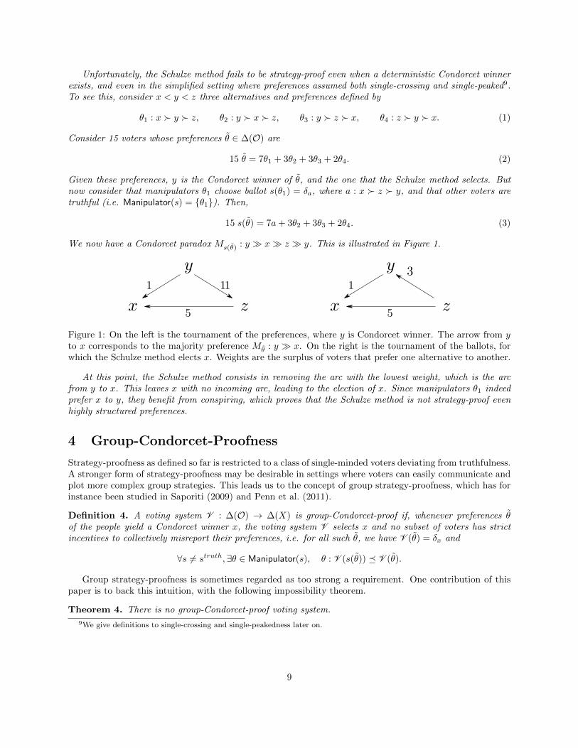
Unfortunately, the Schulze method fails to be strategy-proof even when a deterministic Condorcet winnerexists, and even in the simplified setting where preferences assumed both single-crossing and single-peaked9.To see this, consider x < y < z three alternatives and preferences defined by

θ1 : x � y � z, θ2 : y � x � z, θ3 : y � z � x, θ4 : z � y � x. (1)

Consider 15 voters whose preferences θ ∈ ∆(O) are

15 θ = 7θ1 + 3θ2 + 3θ3 + 2θ4. (2)

Given these preferences, y is the Condorcet winner of θ, and the one that the Schulze method selects. Butnow consider that manipulators θ1 choose ballot s(θ1) = δa, where a : x � z � y, and that other voters aretruthful (i.e. Manipulator(s) = {θ1}). Then,

15 s(θ) = 7a+ 3θ2 + 3θ3 + 2θ4. (3)

We now have a Condorcet paradox Ms(θ) : y � x� z � y. This is illustrated in Figure 1.

Figure 1: On the left is the tournament of the preferences, where y is Condorcet winner. The arrow from yto x corresponds to the majority preference Mθ : y � x. On the right is the tournament of the ballots, forwhich the Schulze method elects x. Weights are the surplus of voters that prefer one alternative to another.

At this point, the Schulze method consists in removing the arc with the lowest weight, which is the arcfrom y to x. This leaves x with no incoming arc, leading to the election of x. Since manipulators θ1 indeedprefer x to y, they benefit from conspiring, which proves that the Schulze method is not strategy-proof evenhighly structured preferences.

4 Group-Condorcet-Proofness

Strategy-proofness as defined so far is restricted to a class of single-minded voters deviating from truthfulness.A stronger form of strategy-proofness may be desirable in settings where voters can easily communicate andplot more complex group strategies. This leads us to the concept of group strategy-proofness, which has forinstance been studied in Saporiti (2009) and Penn et al. (2011).

Definition 4. A voting system V : ∆(O) → ∆(X) is group-Condorcet-proof if, whenever preferences θof the people yield a Condorcet winner x, the voting system V selects x and no subset of voters has strictincentives to collectively misreport their preferences, i.e. for all such θ, we have V (θ) = δx and

∀s 6= struth,∃θ ∈ Manipulator(s), θ : V (s(θ)) � V (θ).

Group strategy-proofness is sometimes regarded as too strong a requirement. One contribution of thispaper is to back this intuition, with the following impossibility theorem.

Theorem 4. There is no group-Condorcet-proof voting system.

9We give definitions to single-crossing and single-peakedness later on.

9

Proof. The proof only requires 4 alternatives and 7 voters, among whom only 2 need to be assumed to bemanipulators. Let X = {w, x, y, z} and the ballots:

a1 : x � y � z � w, a2 : z � x � y � w, (4)

a3 : x � w � y � z, a4 : y � w � z � x, a5 : z � w � x � y. (5)

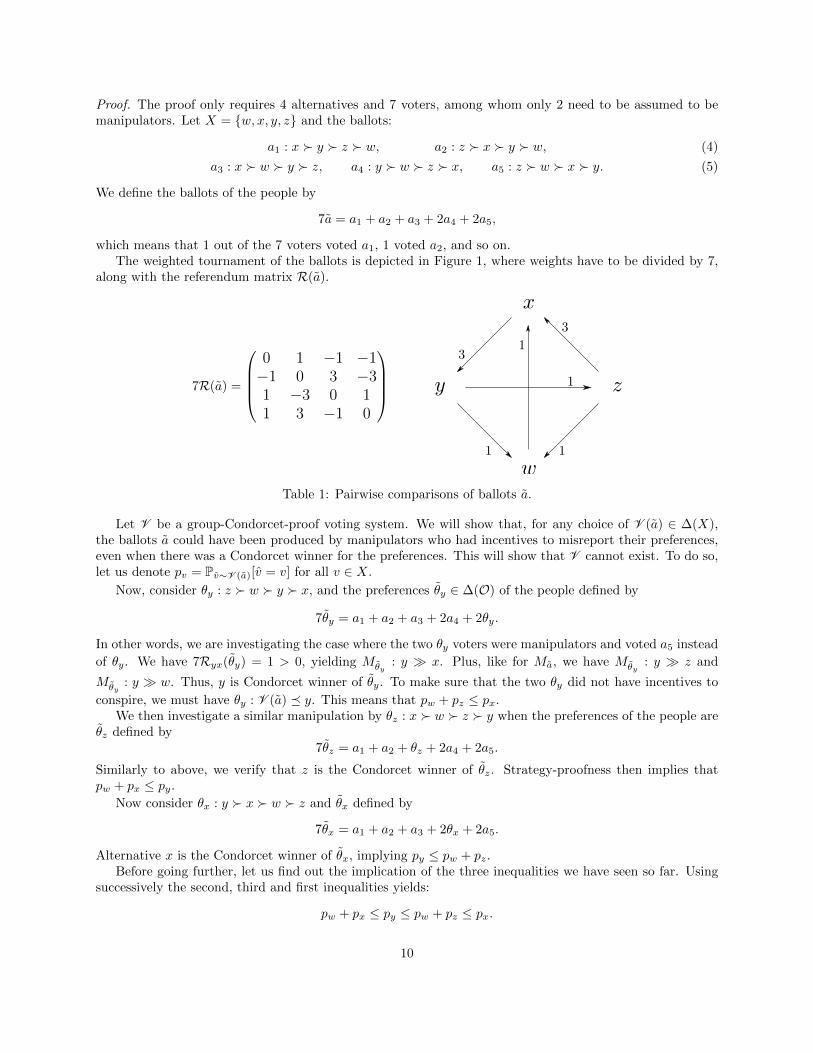
We define the ballots of the people by

7a = a1 + a2 + a3 + 2a4 + 2a5,

which means that 1 out of the 7 voters voted a1, 1 voted a2, and so on.The weighted tournament of the ballots is depicted in Figure 1, where weights have to be divided by 7,

along with the referendum matrix R(a).

7R(a) =

0 1 −1 −1−1 0 3 −31 −3 0 11 3 −1 0

Table 1: Pairwise comparisons of ballots a.

Let V be a group-Condorcet-proof voting system. We will show that, for any choice of V (a) ∈ ∆(X),the ballots a could have been produced by manipulators who had incentives to misreport their preferences,even when there was a Condorcet winner for the preferences. This will show that V cannot exist. To do so,let us denote pv = Pv∼V (a)[v = v] for all v ∈ X.

Now, consider θy : z � w � y � x, and the preferences θy ∈ ∆(O) of the people defined by

7θy = a1 + a2 + a3 + 2a4 + 2θy.

In other words, we are investigating the case where the two θy voters were manipulators and voted a5 instead

of θy. We have 7Ryx(θy) = 1 > 0, yielding Mθy: y � x. Plus, like for Ma, we have Mθy

: y � z and

Mθy: y � w. Thus, y is Condorcet winner of θy. To make sure that the two θy did not have incentives to

conspire, we must have θy : V (a) � y. This means that pw + pz ≤ px.We then investigate a similar manipulation by θz : x � w � z � y when the preferences of the people are

θz defined by7θz = a1 + a2 + θz + 2a4 + 2a5.

Similarly to above, we verify that z is the Condorcet winner of θz. Strategy-proofness then implies thatpw + px ≤ py.

Now consider θx : y � x � w � z and θx defined by

7θx = a1 + a2 + a3 + 2θx + 2a5.

Alternative x is the Condorcet winner of θx, implying py ≤ pw + pz.Before going further, let us find out the implication of the three inequalities we have seen so far. Using

successively the second, third and first inequalities yields:

pw + px ≤ py ≤ pw + pz ≤ px.

10

This leads to pw ≤ 0, and, since probabilities are non-negative, pw = 0. It then follows that px = py = pz =1/3. This determines uniquely the lottery that V (a) must be to guarantee individual Condorcet-proofness.Interestingly, this is precisely the lottery prescribed by the RCVS.

However, we can show that this lottery is not compatible with group-Condorcet-proofness. Indeed,consider θ1w : x � y � w � z and θ2w : z � x � w � y and θw defined by

7θw = θ1w + θ2w + a3 + 2a4 + 2a5.

Now, w is the Condorcet winner of θw. But since we have 2/3 = px + py > pz = 1/3 and 2/3 = px + pz >py = 1/3, both manipulators θ1w and θ2w had incentives to conspire. Thus V is not group-Condorcet-proof,which proves the theorem.

4.1 Median Voter

In practice, many social choice settings yield a natural one-dimensional structure, e.g. in politics. This meansthat alternatives can be located on a one-dimensional line, and that the preferences of voters are somehowconsistent with the way alternatives are located on the line. The one-dimensionality of alternatives can berepresented by a total order relation on X, where x < y means that x is ”on the left” of y. However, inthe literature, we find two distinct definitions of the consistency of preferences with respect to the left-rightstructure of alternatives.

Definition 5. The set OSP of single-peaked preferences is the set of preferences θ such that, denoting x∗(θ)the favorite alternative of θ, we have

(y < x < x∗(θ) or x∗(θ) < x < y) =⇒ θ : x � y,

for any two alternatives x and y.A set OSC of preferences is single-crossing if there is an order relation ”<” on OSC such that, whenever

x1 < x2 and θ1 < θ2, we have(θ1 : x2 � x1 ⇒ θ2 : x2 � x1

)and

(θ2 : x1 � x2 ⇒ θ1 : x1 � x2

).

These two definitions are incompatible, in the sense that there are single-crossing sets of preferences thatdo not satisfy single-peakedness, and the set of single-peaked preferences is not single-crossing. However,under any of these two assumptions, we can define the concept of a median voter10. The well-known medianvoter theorem then holds.

Theorem 5 (Black (1958); Dummett and Farquharson (1961); Roberts (1977); Rothstein (1990, 1991);Gans and Smart (1996)). If preferences are single-peaked or single-crossing and yield a median voter, thenthe median voter’s favorite alternative is the Condorcet winner.

Note that Black (1958) proved that this allows a majority of the people to secure the selection of theCondorcet winner. In other words, if the majority agrees to select the Condorcet winner, no one outsidethe majority can modify the outcome. This property is called stability. Dummett and Farquharson (1961)showed that it still held even if we slightly weaken the single-peakedness assumption. However, stabilityis weaker than strategy-proofness, which requires that no one, within the majority or not, can manipulatethe vote to obtain a better alternative. As pointed out by Penn et al. (2011), the apparent simplicity ofthe theorem above vanishes as we involve strategy-proofness. Indeed, Penn et al. (2011) proved that adeterministic group-strategy-proof voting system must be dictatorial even when preferences are assumedsingle-peaked.

Now, Moulin (1980) did propose a strategy-proof voting system for single-peaked preferences called themedian rule, and Saporiti (2009) did prove the group-strategy-proofness for single-crossing preferences of a

10In the case of single-peakedness, the median voter is ill-defined, but the favorite alternative of the median voter is well-defined, by considering the partial order on voters derived by the left-right order between their favorite alternatives.

11

variant of the median rule. However, to do so, alternatives must officially and unambiguously be locatedon the left-right line, and voters must be forbidden from voting ballots that are inconsistent with this left-right line. In fact, the mere concept of the median voter requires assuming that everyone agrees on howalternatives range on the left-right line. In many cases, e.g. politics, even when alternatives and preferencesmostly have some hidden left-right structure, alternatives may refuse to be located on this left-right line,and voters may refuse to be forbidden from casting non-single-crossing or non-single-peaked ballots.

Formally, this would require to define a voting system V : ∆(Θ) → ∆(X), even though we believe orknow the support of θ to be restricted to OSP or some OSC . In particular, manipulations may still produceballots s(θ) whose support is not limited to OSP or some OSC , in which case a decision V (s(θ)) still needsto be made.

This subtle difficulty to design strategy-proof voting systems even under one-dimensional preferencesrenders methods by Moulin (1980) and Saporiti (2009) inapplicable in our setting. Meanwhile, we have seenin Example 5 that the Schulze method fails to be strategy-proof even when preferences are both single-peakedand single-crossing. This makes the following result all the more remarkable.

Theorem 6. When the support of the preferences θ is single-peaked or single-crossing, the RCVS is groupCondorcet-proof.

The proof is given in Appendix B.

5 Conclusion

In this paper, we have unveiled some remarkable strategy-proof properties of the RCVS. Namely, we haveproved the RCVS is Condorcet-proof, and that, in a large class of voting systems, it is the only one to beCondorcet-proof. Moreover, when preferences are one-dimensionsal, it is even group-Condorcet-proof. Wehave shown this to be a remarkable property by proving that, in the general case, there is no group-Condorcet-proof voting system. Given that, in addition, the RCVS is a natural and easily computable extension ofCondorcet’s ideas, it is tempting to assume that, considering Condorcet’ philosophical take on social choicetheory, his wide use of probability theory in diverse problems, and his concern of strategy-proofness, ”hewould have endorsed [the RCVS] enthusiastically”, as already noted by Felsenthal and Machover (1992). Forthese reasons, we end this paper by emphatically advocating its use in practice.

Acknowledgements I am greatly grateful to Remi Peyre without whom this paper would not havebeen possible. He introduced me to social choice theory in popularized articles Peyre (2012a,b,c). Second,he sketched the proof of Theorem 2, and hinted at Theorem 3. Finally, and most importantly, our discussionsgave me great insights into the wonderful theory of voting systems. I am also grateful to anonymous refereesas well as the managing editor, who provided useful references and remarks that greatly simplified andclarified the exposition of this work.

References

K. Arrow. Individual values and social choice. Nueva York: Wiley, 24, 1951.

H. Aziz, F. Brandt, and M. Brill. On the tradeoff between economic efficiency and strategy proofness inrandomized social choice. In Proceedings of the 2013 International Conference on Autonomous Agents andMulti-Agent Systems, pages 455–462, 2013.

H. Aziz, F. Brandl, and F. Brandt. On the incompatibility of efficiency and strategyproofness in randomizedsocial choice. In Proceedings of 28th Association for the Advancement of Artificial Intelligence Conference,pages 545–551, 2014.

H. Aziz, F. Brandl, and F. Brandt. Universal pareto dominance and welfare for plausible utility functions.Journal of Mathematical Economics, 60:123–133, 2015.

12

I. Balbuzanov. Convex strategyproofness with an application to the probabilistic serial mechanism. SocialChoice and Welfare, 46(3):511–520, 2016.

D. Black. The Theory of Committees and Elections. Cambridge, England, Cambridge University Press, 1958.

A. Bogomolnaia and H. Moulin. A new solution to the random assignment problem. Journal of Economictheory, 100(2):295–328, 2001.

A. Bogomolnaia, H. Moulin, and R. Stong. Collective choice under dichotomous preferences. Journal ofEconomic Theory, 122(2):165–184, 2005.

F. Brandl, F. Brandt, and H. G. Seedig. Consistent probabilistic social choice. Econometrica, 84(4):1839–1880, 2016.

D. E. Campbell and J. S. Kelly. Incompatibility of strategy-proofness and the condorcet principle. SocialChoice and Welfare, 15(4):583–592, 1998.

S. Chatterji, A. Sen, and H. Zeng. Random dictatorship domains. Games and Economic Behavior, 86:212–236, 2014.

M. J. A. N. d. C. Condorcet. Essai sur l’application de l’analyse a la probabilite des decisions rendues a lapluralite des voix. L’Imprimerie Royale, 1785.

M. Dummett and R. Farquharson. Stability in voting. Econometrica: Journal of the Econometric Society,pages 33–43, 1961.

L. Ehlers, H. Peters, and T. Storcken. Strategy-proof probabilistic decision schemes for one-dimensionalsingle-peaked preferences. Journal of Economic Theory, 105(2):408–434, 2002.

D. S. Felsenthal and M. Machover. After two centuries, should Condorcet’s voting procedure be implemented?Behavioral Science, 37(4):250–274, 1992.

P. C. Fishburn. Nontransitive measurable utility. Journal of Mathematical Psychology, 26(1):31–67, 1982.

P. C. Fishburn. Probabilistic social choice based on simple voting comparisons. The Review of EconomicStudies, pages 683–692, 1984.

D. C. Fisher and J. Ryan. Optimal strategies for a generalized ”scissors, paper, and stone” game. TheAmerican Mathematical Monthly, 99(10):935–942, 1992.

J. S. Gans and M. Smart. Majority voting with single-crossing preferences. Journal of Public Economics,59(2):219–237, 1996.

A. Gibbard. Manipulation of voting schemes: a general result. Econometrica: Journal of the EconometricSociety, pages 587–601, 1973.

A. Gibbard. Manipulation of schemes that mix voting with chance. Econometrica: Journal of the Econo-metric Society, pages 665–681, 1977.

A. Gibbard. Straightforwardness of game forms with lotteries as outcomes. Econometrica: Journal of theEconometric Society, pages 595–614, 1978.

J. Grime. Non-transitive dice, 2010. URL http://singingbanana.com/dice/article.htm.

G. Kreweras. Aggregation of preference orderings. In Mathematics and Social Sciences I: Proceedings of theSeminars of Menthon-Saint-Bernard, France (1–27 July 1960) and of Gosing, Austria (3–27 July 1962),pages 73–79, 1965.

13

G. Laffond, J.-F. Laslier, and M. Le Breton. The bipartisan set of a tournament game. Games and EconomicBehavior, 5(1):182–201, 1993.

J.-F. Laslier. Tournament solutions and majority voting. Number 7. Springer Verlag, 1997.

J.-F. Laslier. Aggregation of preferences with a variable set of alternatives. Social Choice and Welfare, 17(2):269–282, 2000.

H. Moulin. On strategy-proofness and single peakedness. Public Choice, 35(4):437–455, 1980.

R. B. Myerson. Fundamentals of social choice theory. Center for Mathematical Studies in Economicsand Management Science, Northwestern University, 1996. URL http://home.uchicago.edu/rmyerson/

research/schch1.pdf.

J. Nash. Non-cooperative games. Annals of Mathematics, pages 286–295, 1951.

E. M. Penn, J. W. Patty, and S. Gailmard. Manipulation and single-peakedness: A general result. AmericanJournal of Political Science, 55(2):436–449, 2011.

R. Peyre. La democratie, objet detude mathematique. Images des Mathematiques, CNRS, 2012a. URLhttp://images.math.cnrs.fr/La-democratie-objet-d-etude.html.

R. Peyre. Et le vainqueur du second tour est... Images des Mathematiques, CNRS, 2012b. URL http:

//images.math.cnrs.fr/Et-le-vainqueur-du-second-tour-est.html.

R. Peyre. La quete du graal electoral. Images des Mathematiques, CNRS, 2012c. URL http://images.

math.cnrs.fr/La-quete-du-Graal-electoral.html.

R. L. Rivest and E. Shen. An optimal single-winner preferential voting system based on game theory. InProc. of the 3rd Intl. Workshop on Computational Social Choice (COMSOC), pages 399–410. Citeseer,2010.

K. W. Roberts. Voting over income tax schedules. Journal of Public Economics, 8(3):329–340, 1977.

P. Rothstein. Order restricted preferences and majority rule. Social Choice and Welfare, 7(4):331–342, 1990.

P. Rothstein. Representative voter theorems. Public Choice, 72(2-3):193–212, 1991.

A. Saporiti. Strategy-proofness and single-crossing. Theoretical Economics, 4(2):127–163, 2009.

M. A. Satterthwaite. Strategy-proofness and arrow’s conditions: Existence and correspondence theorems forvoting procedures and social welfare functions. Journal of Economic Theory, 10(2):187–217, 1975.

M. Schulze. A new monotonic, clone-independent, reversal symmetric, and condorcet-consistent single-winnerelection method. Social Choice and Welfare, 36(2):267–303, 2011.

J. Von Neumann. Die zerlegung eines intervalles in abzahlbar viele kongruente teilmengen. FundamentaMathematicae, 11(1):230–238, 1928.

J. Von Neumann and O. Morgenstern. Theory of games and economic behavior. Princeton University Press,1944.

14

A Proof of Theorem 3

First, we notice that ∆(O) can be regarded as the simplex of RO, and that the map R : ∆(O)→ RX×X canbe uniquely extended to a linear map R : RO → RX×X . This linear map has the two following properties.

Lemma 2. The image of R coincides with the space of skew-symmetric matrices11.

Proof. It is straightforward to see that the image of R is included in the space of skew-symmetric matrices.Reciprocally, to show the equality, we need only show that any element of the canonical basis of skew-symmetric matrices is in the image of referendum. Such an element R ∈ RX×X is of the form Rxy = −Ryx = 1for some two different alternatives x, y ∈ X, and Rvw = 0 in any other case. Denote v1, . . . , vn the otheralternatives. We define θ ∈ RO by θ = (θ1 + θ2)/2, where

θ1 : x � y � v1 � . . . � vn and θ2 : vn � . . . � v1 � x � y.

We then have Rvw(θ) = 0 if (v, w) /∈ {(x, y), (y, x)} and Rxy(θ) = −Ryx(θ) = 1, which proves that

R = R(θ).

Lemma 3. R(∆(O)) contains all skew-symmetric matrices of `1-norm at most 2.

Proof. In the proof of Lemma 2, we showed that each element of the canonical basis is the image R(θ) ofsome preferences θ ∈ ∆(O) of the people. Yet, such elements of the canonical basis are of `1-norm 2. SinceR is linear and ∆(O) convex, R(∆(O)) therefore contains all convex combinations of the elements of thecanonical basis of skew-symmetric matrices. Plus, since, for any two distinct matrices of the canonical basis,the norm of the sum is the sum of the norms, all skew-symmetric matrices of `1-norm 2 are images by R ofsome preferences of ∆(O). Plus, the uniform distribution u ∈ ∆(O) on all ballots is trivially in the kernelof R. A convex combination involving u then enables to obtain any skew-symmetric matrix of `1-norm atmost 2.

We still need another lemma before proving the theorem.

Lemma 4. Let the preferences θ ∈ ∆(O), the ballots a ∈ ∆(O) and a subset C ⊂ O of manipulators. Then,there exists a strategy s ∈ S such that s(θ) = a and Manipulator(s) = C if and only if Pθ[D] ≤ Pa[D] for all

subsets D ⊂ O − C. In particular, if X is finite, this condition amounts to Pθ(θ = a) ≤ Pa(a = a) for alla /∈ C.

Proof. First notice that θ could have produced a with a set C of manipulators if and only if there exists astrategy s such that Manipulator(s) = C and s(θ) = a. Consider that we indeed have s(θ) = a, and let usprove the direct implication of the lemma. Let D ⊂ O − C. Then,

Pa[D] = Eθ[Ps(θ)[D]

]= Eθ

[Ps(θ)[D]

∣∣∣θ ∈ D]Pθ[D] + Eθ[Ps(θ)[D]

∣∣∣θ /∈ D]Pθ[O −D].

But since D ∩ C = ∅, for all θ ∈ D, we have θ /∈ C. Thus, s(θ) = struth(θ) = δθ. Thus, Ps(θ)[D] = 1. Thus,the expression above simplifies to

Pa[D] = Pθ[D] + Eθ[Ps(θ)[D]

∣∣∣θ /∈ D]Pθ[O −D].

Therefore, Pa[D] ≥ Pθ[D], hence proving the direct implication.

Reciprocally, if Pθ[C] = 0, then the inequality Pθ[D] ≥ Pa[D] implies θ = a. Thus, struth(θ) = a, which

proves that θ could have produced a with the set C of manipulators. Otherwise, Pθ[C] 6= 0. We defines : C → ∆(O) by Ps(θ)[C − {θ}] = 0,

1. ∀E ⊂ C,Ps(θ)[E ] = Pa[E ]/Pθ[C].11A skew-symmetric matrix R is a matrix whose transposition RT equals its opposite −R, i.e. RT = −R

15

2. ∀D ⊂ O − C,Ps(θ)[D] =(Pa[D]− Pθ[D]

)/Pθ[C].

Assuming Pθ[D] ≤ Pa[D] for all supsets D ⊃ O−C, the probabilities we have defined here are all non-negative.It is straightforward to see that the additivity of the probability is satisfied. Plus,

Pθ[O] = Pθ[C] + Pθ[O − C) =Pa[C]Pθ[C]

+Pa[O − C)− Pθ[O − C]

Pθ[C]= 1.

Therefore, s(θ) is a well-defined probability, and s a well-defined strategy of support C. Plus, for D ⊂ O−C,

Ps(θ)[D] = Pθ[D] + Eθ[Ps(θ)[D]

∣∣∣θ ∈ C]Pθ[C] + Eθ[Ps(θ)[D]

∣∣∣θ /∈ C ∪ D]Pθ[O − C ∪ D]

= Pθ[D] +Pa[D]− Pθ[D]

Pθ[C]Pθ[C] = Pa[D],

and, similarly for any E ⊂ C, we have

Ps(θ)[E ] = Eθ[Ps(θ)[E ]

∣∣∣θ ∈ C]Pθ[C] =Pa[E ]

Pθ[C]Pθ[C] = Pa[E ].

These two equalities prove that s(θ) = a, which is what we had to prove.

We can now prove Theorem 3.

Theorem 3. By contradiction, assume that V disagrees with the RCVS C for some referendum matrix R of`1-norm less than 2. Let us consider ballots a+vw, a

−vw ∈ O defined by

a+vw : v � w � x1 � . . . � xn and a−vw : xn � . . . � x1 � v � w.

Like in the proof of Lemma 2, the choices of x1, . . . , xn are irrelevant. What matters to us is the fact thatR(a+vw + a−vw) is a skew-symmetric matrix of the canonical basis. In particular, the referendum matrix Rthat the pairwise voting system is based on can be obtained from the ballots a defined by

a =1

2

∑v,w:Rvw>0

Rvwa+vw +

1

2

∑v,w:Rvw>0

Rvwa−vw + δu,

where δ = 1− 12 ||R||1. By assumption on R, we have δ > 0.

Since, by assumption, Rxy 6= 0 for all x 6= y, the ballots a yields a unique randomized Condorcet winner.Therefore, the fact that V disagrees with C on R implies that V (a) is not the randomized Condorcet winnerof a. In other words, there must be some alternative x ∈ X that the majority Ma strictly prefers to V(a).Denoting Z = {z1, . . . , zn} and Y = {y1, . . . , ym} the sets of alternatives that the majority Ma respectivelyprefers x to (Ma : x� z) and prefers to x (Ma : y � x), this means that PV (a) [Z] > PV (a) [Y ]. Evidently,by definitions of sets Y and Z, we have Ryx > 0 and Rxz > 0 for all y ∈ Y and z ∈ Z.

We then define the preference θ ∈ O of manipulators by

θ : z1 � . . . � zn � x � y1 � . . . � ym.

Notice that we have θ : V (a) � x. We can now define the preferences θ ∈ ∆(O) of the people by

θ =1

2

∑Ma:v�w

(v,w)/∈Y×{x}

Rvw(a+vw + a−vw) +1

2

∑y∈Y

Ryxa+yx +

ε+1

2

∑y∈Y

Ryx

θ + (δ − ε)u,

16

with 0 < ε < δ. Importantly, any ballot a ∈ O except θ is more frequent in a than in θ. Thus, by Lemma 4,manipulators θ can have produced the ballots a. Moreover, we have:

∀z ∈ Z, Rxz(θ) = Rxz+1

2

∑y∈Y

Ryx −ε− 1

2

∑y∈Y

Ryx = Rxz −ε,

∀y ∈ Y, Rxy(θ) = −1

2

∑y∈Y

Ryx +ε+1

2

∑y∈Y

Ryx = +ε.

Recall that Rxz > 0 for all z ∈ Z, hence we can choose ε smaller than all Rxz. By doing so, we guaranteethat Rxz(θ) and Rxy(θ) are positive for all z ∈ Z and y ∈ Y . Thus, x is a Condorcet winner for θ. Yet, bycreating ballots a, manipulators θ have obtained strictly better, as we have seen that θ : V (a) � x. Thisshows that V is not Condorcet-proof. This proves that a Condorcet-proof pairwise voting system must agreewith the RCVS whenever ||R(θ)||1 < 2.

The uniqueness of Condorcet-proof tournament-based voting system is then immediately derived byconsidering any skew-symmetric matrix R0, and by dividing each entry by the `1-norm of the matrix, henceyielding a skew-symmetric matrix R of norm 1 to which the previous part applies.

B Proof of Theorem 5

We first prove the following lemma about the structure of the set of manipulators when preferences areone-dimensional.

Lemma 5. When preferences are single-peaked or single-crossing with a unique median voter, manipulatorsmust either be all strictly on the left or all strictly on the right of the median voter.

Proof. Let V a voting system. Denote x the Condorcet winner of the single-peaked preferences θ ∈ ∆(O).Denote Z and Y the sets of alternatives that are respectively on the left and on the right of x. Now, considera strategy s. We denote s(θ) = a. The strict incentive to conspire means that

∀θ ∈ Manipulator(s), θ : V (a) � x.

If preferences are single-peaked or single-crossing and θ ∈ Manipulator(s) is on the right of the median voter,we know that θ : x � z for all z ∈ Z. Indeed, if preferences are single-peaked, this is due to θ’s ideal pointbeing on the right of x. And if preferences are single-crossing, this is because x cannot be switched with aleft alternative as we look preferences on the right of the median voter. Since the median voter ranked xbetter than any z ∈ Z, all voters on its right must do so too.

Thus, {z ∈ X | θ : x � z} ⊃ Z, and, as a result, {y ∈ X ‖ θ : y � x} ⊂ Y . Therefore,

0 < Pv∼V (a) [θ : v � x]− Pv∼V (a) [θ : v ≺ x] ≤ PV (a)[Y ]− PV (a)[Z].

Therefore, we have PV (a)[Y ] > PV (a)[Z]. But if θ ∈ Manipulator(s) is on the left of the median voter, we musthave the opposite inequality. Both cases cannot occur simultaneously, which proves that all manipulatorsmust be on the same side of the left-right spectrum with regards to the median voter. This proves thelemma.

We can now prove Theorem 5. The proof slightly differs depending on the assumption of one-dimensionalityof preferences that is considered. For clarity, we write the proofs of the two cases in separate blocks.

Theorem 5 for single-peakedness preferences. Let C denote the randomized Condorcet voting system. Weuse the same notations x, θ, Y, Z, s and a as in the proof of Lemma 5. Without loss of generality, we canassume that manipulators are all strictly on the right of the median voter.

Let z ∈ Z. As we have seen in the previous proof, we have θ : x � z for all θ ∈ Manipulator(s). Sincemanipulators agree with Mθ : x � z for z ∈ Z, according to Lemma 1, they cannot invert these pairwise

17

comparisons. Therefore, Ma : x� z. Yet, for manipulators to gain by conspiring, C (a) must differ from x,which means that there must be some y ∈ Y such that Ma : y � x. Let y∗ the most leftist alternative thatthe majority of ballots prefers to x, i.e.

y∗ = min{y ∈ Y |Ma : y � x},

where the minimum corresponds to the order relation ”<” on alternatives. We denote Y− , {y− ∈ Y | x <y− < y∗} and Y+ , Y − Y− = {y+ ∈ Y | y∗ ≤ y+}.

Since x is Condorcet winner of θ, we know that Mθ : x � y∗. Thus, manipulators must have invertedthe majority preference of x over y∗. Since, according to Lemma 1, manipulators can only invert arcs theyagree with, this means that there must be a manipulator θ ∈ Manipulator(s) who agrees with Mθ : x � y∗.This manipulator thus thinks θ : x � y∗. We will show that assuming that he had incentive to conspire leadsto a contradiction.

On one hand, by definition of y∗, we have Ma : x� y for all y ∈ Y−, i.e.

Y− ⊂{w ∈ X |Ma : x� w

}and {w ∈ X |Ma : w � x} ⊂ Z ∪ Y+.

Combining this with the property Ma : C (a) � x satisfied by the randomized Condorcet voting systemyields

PC (a)[Y−] ≤ Pw∼C (a) [Ma : x� w]

≤ Pw∼C (a) [Ma : w � x]

≤ PC (a) [Z ∪ Y+] .

On the other hand, strict incentives to conspire for θ imply that

Pw∼C (a) [θ : w � x] > Pw∼C (a) [θ : x � w] .

Since θ : x � y∗, we know that the ideal point of θ is necessarily on the left of y∗. As a result, for y ∈ Y+,we have θ : x � y∗ � y. Therefore,{

w ∈ X | θ : x � w}⊃ Z ∪ Y+ and Y− ⊃

{w ∈ X | θ : w � x

},

which leads to PC (a)[Y−] > PC (a) [Z ∪ Y+]. This contradicts equation (??), and proves the theorem forsingle-peaked preferences.

Theorem 5 for single-crossing preferences. We reuse the same notations x, θ, Y, Z, s and a as in the proofof Lemma 5. Let θm the median voter. Lemma 5 allows us to assume without loss of generality that themanipulators are all on the right of θm, i.e. θ > θm for all θ ∈ Manipulator(s). Then, we have, once again,Ma : x� z for all z ∈ Z.

Let now θ = min Manipulator(s) the most leftist manipulator. Denote Y + and Y − defined by

Y + = {y ∈ Y | θ : y � x} and Y − = {y ∈ Y | θ : x � y}.

Contrary to the proof for single-peakedness, Y + now corresponds to the alternatives some manipulatorsprefer to x, as the sign ” + ” now refers to θ’s preference rather than the left-right line of alternatives.

Let y+ ∈ Y +. Since for any θ′ ∈ Manipulator(s), we have θ < θ′, single-crossing implies that θ′ : y+ � x.Therefore, manipulators all disagree with the majority preference Mθ : x � y+, and hence, by Lemma 5,cannot invert it. Therefore, Ma : x� y+. Since this holds for all y+ ∈ Y +, we have

Y + ⊂ {w ∈ X |Ma : x� w} and {w ∈ X |Ma : w � x} ⊂ Z ∪ Y −.

Yet, the fundamental property of the RCVS applied to x then implies

PC (a)[Y+] ≤ Pw∼C (a) [Ma : x� w]

≤ Pw∼C (a) [Ma : w � x]

≤ PC (a)

[Z ∪ Y −

].

18

But this contradicts the strict incentives for θ to conspire, i.e. PC (a)[Y+] > PC (a) [Z ∪ Y −]. Thus, we reach

the same conclusion for single-crossing preferences as we did for single-peaked ones.

19