Department Socioeconomics

The Real Income Shares of Labor, Human and Physical Capital: Determination Method and First Results for Germany

Peter E. J. Steffen

DEP (Socioeconomics) Discussion Papers Macroeconomics and Finance Series 2/2013

Hamburg, 2013

The Real Income Shares of Labor, Human and

Physical CapitalDetermination Method and First Results for Germany∗

Peter E. J. Steffen†

University Hamburg

February 15, 2013

Abstract

A method is presented that allows to separate the total labor income into parts of basiclabor and human capital using annual micro data. As results yearly total income shares ofphysical and human capital and labor are obtained for a single country.

The method is applied to Germany using micro data of the years 1976, 1985, 1995, and2006. The obtained average income shares are in agreement with the well known results ofMankiw, Romer and Weil [8] if only employed workers are considered.

If self-employed labor is also taken into account, the share ratios of physical and humancapital and labor change to sK : sH : sL = 0.18 : 0.26 : 0.55. This result differs considerablyfrom the generally expected share ratios for developed countries of 1/3 : 1/3 : 1/3.

Further on, the development of the German income shares are investigated. The observedvariation is in contradiction to a constant behavior as expected from Kaldor’s stylized facts.The source could be traced to considerable changes in the qualification structure of the Ger-man work force.

Keywords: human capital, Mikrozensus, annual factor income shares, factor share develop-ment

JEL classification: D33, E25, J24

∗The author would like to thank very much Ulrich Fritsche from University Hamburg for his continuous helpful dis-

cussions over the whole period of this work. Further on he thanks Michael Schmaus and his group from the office of the

Forschungsdatenzentrum der Statistischen Landesamter in Dusseldorf for the discussions on the details of the Mikrozensus

data. The research of this paper was supported by the Statistisches Bundesamt by providing the Mikrozensus data.†Peter E. J. Steffen: email Peter.Steffen@wiso.uni-hamburg.de

1

1 Introduction

Considering only capital K and labor L as production factors their total income shares - sK and sL - arefound to be constant. For the USA one finds sL : sK ≈ 2/3 : 1/3 [5]. A similar behavior is observed forother industrial countries.

In 1992 Mankiw, Romer and Weil [8] showed that human capital H is a further important productionfactor that needs considering. They assumed a Cobb-Douglas production function with production factorsK, H, and A·L (A being a Harrods-neutral technical progress that results in an enhanced L-wage). Theyanalyzed economic data of 98 different countries from 1960 - 1985. They obtained ratios of income sharessK : sH : sL compatible with equal shares of 1/3. Their final conclusion was that H as production factoris necessary to explain cross country differences.

Human capital is considered to be the dominant driving force of economic growth. According to Le,Gibson and Oxley [7] the determination of H is essential in order to establish the correlation between Hand growth. Folloni and Vittadini [3] have provided an extensive survey on procedures for human capitalmeasurements. They differentiated 5 methods for obtaining a measure of H:

1. retrospective method:measure of H is the present value of the costs of formation of the current stock of H,

2. prospective method:measure of H is the present value of the lifelong income of the workers,

3. individual investments:measure of H is w(s,x), the wage as function of the number of schooling years (s) and the numberof years with professional experience (x),

4. educational attainment level:possible measures of H are attainment levels, like fractions of population above certain educa-tional level (e.g. reading capability), GDP-fraction of educational costs, ratio of teachers perpupil/student,

5. H as latent variable:there is no direct measure of H; instead it is assumed to be an unknown function of several qualitativeand quantitative parameters.

All these different methods aim at determining measures of the aggregate H. The result of empiricalstudies of a correlation with economic growth are controversial or insignificant (see e.g.[6]). Folloniand Vittadini state[3](p. 265): “Empirical studies have demonstrated the existence of wide differencesbetween micro analysis (micro data) and those of macro ones. Micro data find substantially positiveimpact of educational attainment on earnings; macro studies show very controversial results”. The originis probably the qualitative difference between economic growth (a dynamic variable) and aggregate H (arather constant variable w.r.t. growth). Therefore the main mode of operation of H is believed to workvia external effects. These are difficult to determine and to valuate.

A possible alternative has been proposed by the OECD [13]: the ratio of higher educated to lowereducated workers may serve as measure of H of the higher educated workers. As result one could obtaina value for the human capital stock: “by weighting different segments of the workforce by the ratio ofearnings at different levels of education, it is possible to derive an index of the value of average humancapital stock” (p.28).

A similar approach for measuring the level of H has been proposed by Mulligan and Sala-i-Martin [12].They use the total income ratio of all workers and those without schooling as measure of the aggregatevalue of H. So the income of workers with no education serves as unit. This is based on the assumptionthat a person without schooling is the same always and everywhere. They further assume that the suchdetermined H is a measure of the aggregate H.

1

B. Jeong [4] developed this method further in order to compare H across countries implying, however,more stringent assumptions, like a fixed income share of H independent of time and country.

However, also these approaches assume to determine a measure of the aggregate value of H.

In this paper - in contrast to the above approaches - H is restricted to its productively used fraction,a small part of the aggregate H. It increases the productivity of workers and results in a higher wage.This has been shown by Jacob Mincer [11] (and others later on) who demonstrated a positive relationbetween wage and the years of education and work time.

The productively used H is expected to show a dynamic behavior similar to economic growth: itcan be increased in rather short time by activation of yet unused parts of H for production, while theaggregate H remains with little changes.

In the following a method is presented for separating the wage (W) into components of basic wage(wo) from pure labor and a surplus wage from the use of human capital in production (wh) (chapter2.1). Yearly micro data are used to determine W from the wage of all employed workers and wo fromthe wage of workers with a minimum of schooling and without professional training. These workers didnot invest in H and therefore are assumed to earn no surplus wage from productively used H. wh, thesurplus wage, is obtained from the difference: wh = W −wo.

The fractions fo = wo / W and fh = wh / W are used to separate the usual labor share of theNNP (net national product), the total income of the economy, into the shares of basic labor and humancapital. This procedure is expected to transfer the correlation between H and income from the microto the macro level: H-investment and earnings (micro level) to the H-share of total income (sH) (macrolevel). The size of sH demonstrates the importance of H for the growth of NNP resp. GDP.

The value of sH itself is suited to be a measure of the productively used H in units of the NNP of theeconomy. Annual measures together with sK and sL will serve in understanding the development of asingle economy.

Details of the determination of wages and total income shares are described in chapter 2.2, followedby a discussion of the method (chapter 2.3).

As an example the German Mikrozensus (MZ) data of 1976, 1985, 1995 and 2006 are used in orderto determine the wage parameters W, wo, wh, fo and fh (chapter 3.1).

First the wage parameters of the employed workers and self-employed are determined (chapter 3.2).Then the wage parameters are used for the determinations of the NNP shares (chapter 4). At first onlythe L-share of the employed workers (EL) is separated into sL(EL) and sH(EL). The resulting data(chapter 4.1) are compared and found to be in agreement with the MRW-results [8].

Further on the labor and human capital shares of the self-employed workers (SE) are determined(chapter 4.2). In general they are included in the K-share. A separation from the K-share does yield thereal sK without admixtures of L and H. It also yields the real shares sH and sL (including contributionsof EL and SE).

Significant differences w.r.t. the generally expected ratio of 1/3 : 1/3 : 1/3 are observed and dis-cussed.

The German development from 1976 - 2006 does show a considerable variation in time. This is incontradiction to a constant behavior as expected for developed countries like Germany. This behavior isinvestigated further using detailed micro data of different groups of qualification (chapter 4.3).

Finally the results for Germany are discussed in chapter 5.

2

2 Method for Separating the Wage Components of Basic Labor

and Human Capital

2.1 Theoretical Background

In this chapter a method is described that allows the simultaneous determination of a basic labor wageand the surplus wage that is payed depending on the productive use of individual human capital.

Following Mankiw, Romer and Weil [8] a production function with the the factors K, H, L and anexogenous technology A is considered:

Y = F(K, H, AL)

r · K + rh · H + Aw · L. (2.1)

It should be noted that Y stands for the NNP, the total income of the production factors. The difference tothe GDP is essentially due to depreciation of K and the balance of duties and subsidies of the firms. Theseare not accounted in the NNP in order to put all production factors onto the same footing. (Otherwisedepreciation and the balance of duties and subsidies would count as additional rent of K.) In this waythe NNP serves as reference value for the shares of the production factors.Further details are described in appendix A.1.

At the microeconomic level the individual worker earns a basic wage wo plus a surplus wage wh

depending on his individual human capital engagement:

W(i) = wo + wh(i) (total wage of indiv. worker i) (2.2)

So a worker without any human capital engagement will earn only the basic wage wo. This fact is usedto determine wo: the wage of workers without schooling and professional qualification.

At the macroeconomic level the mean human capital is used:

Y = r · K +

L∑

i=1

wh(i) + wo · L (2.3)

r · K + wh · L + wo · L (2.4)

Y(sK + sH + sL), (2.5)

where wh is the mean of the individual wh(i), and sK, sH and sLare the NNP shares. The sum inequation 2.3 is the rent obtained from productively used H.

A simultaneous determination of the total wage W and wo yields wh = W − wo. Also the wagefractions fo = wo / W and fh = wh / W are determined. They are used in separating the labor incomeinto contributions from H and L.

It should be noted that the assumed Harrods neutral technology implies factor neutrality. In case ofnon neutrality there will be efficiency differences between all production factors. In this case the differentfactor shares may have technology enhanced return rates.

2.2 Determination of Wages and Income Shares

The wages are determined from income distributions. The income is stated as monthly or annual incomein the micro data. They have to be converted to hourly wages. This will yield results independent ofvariations in working time which depends on individual choice or general agreements.

The labor income is stated in the micro data only for the EL (employed worker). The labor income ofSE (self-employed) is part of their total income that also comprises the rent of their investments. Theirlabor income has to be estimated.

The following procedure is used:

3

1. determine the wages W, wo, wh and the wage fractions fo and fh for the EL using the incomedistributions from the micro data.

2. estimate the labor wages and wage fractions of the SE. Here the assumption Wq(SE) = Wq(EL) isused; so SE and EL of the same qualification get the same wage per hour. The following argumentsapply: the self-employed wage is certainly not lower, otherwise the running of ones own firm wouldnot make sense; it might be higher because of a higher efficiency, but this is not accessible and isascribed to individual investment.

In case of a minimum qualification the above assumption yields

Wq min(EL) = wo(EL) = wo(SE) = wo , (2.6)

so the basic wages of EL and SE are identical. It is determined from the EL-data.

W(SE) is determined using wage distributions of the EL, weighted according to the qualificationstructure of the self-employed. Starting point are the wage distributions of employed workersseparate for different qualifications q:

{nq(wi)}EL (2.7)

with nq being the number of entries in wage-bin wi. These distributions are added with weightsthat reflect the differences in qualification between EL and SE:

{n(wi)}SE =∑

q

{nq(wi)EL} ·Nq(SE)

Nq(EL)(2.8)

with Nq being the number of worked hours of SE and EL. The such obtained wage distribution ofSE is used for determining W(SE) in the same way as W(EL) has been obtained.

After this procedures W and wo of EL and SE are available for use as input data in the calculation ofthe NNP shares of K, H and L.

Further input data are the published annual income share of the EL. These are part of the annual eco-nomic summary data provided by statistical institutes, e.g. for Germany the VGR (VolkswirtschaftlicheGesamtrechnung) of the “Statistisches Bundesamt” [15],[17]. Part of these data are the NNP and itsshares of labor and capital: sK(VGR) and sL(VGR), wheresL(VGR)comprises the sum of sL(EL) and sH(EL) andsK(VGR)comprises sK and the sum of sL(SE) and sH(SE).

The shares of the EL are obtained with

sL(EL) = fo(EL) · sL(VGR) and (2.9)

sH(EL) = fh(EL) · sL(VGR), (2.10)

so sL(VGR) is divided up by using the wage ratios fo and fh of the EL.The labor income shares of the SE are determined as follows

sL(SE) = sL(EL) ·N(SE) · hw(SE)

N(EL) · hw(EL)(2.11)

sH(SE) = sL(SE) ·wh(SE)

wo

(2.12)

First the basic labor share sL(SE) is determined by scaling sL(EL) with the ratio of numbers (N) andweekly working hours (hw) of SE to EL.Second the human capital share sH(SE) is determined from sL(SE) by using the ratio of wh / wo.

4

Finally the real NNP shares of the production factors L, H, K are then obtained by

sL = sL(EL) + sL(SE) (2.13)

sH = sH(EL) + sH(SE) (2.14)

sK = 1 − sL − sH (2.15)

They are called “real” because they are complete shares of the corresponding production factors andthey do not contain admixtures from other production factors.

Without the separation of sK (from the labor of the self-employed) sK would depend on individualdecisions to work as employed or self-employed. This decision is influenced by taxes and regulations.This influence on the shares of production factors is avoided by the above procedure.

Further on the income per person (IPP) of the different production factors can be derived from thereal income shares:

IPPL = sL · NNP/P (2.16)

IPPH = sH · NNP/P (2.17)

IPPK = sK · NNP/P (2.18)

where P stands for the population.In an analogous way IPW can be defined, the income per worker using NNP/worker. These variables

can serve as measure of productivity of the production factors in a comparison of different countries.

2.3 Discussion of the Method

The assumptions are:

• there are 3 production factors K, H, L that determine the total output of a country,

• a basic labor income wo is earned by persons of minimal qualification: they did not invest in H(education or professional qualification),

• persons that have invested in H do earn a surplus wage wh that is proportional to their productivelyused H

• the wage ratios fo and fh of the EL can be applied to the total labor share yielding sL(EL) andsH(EL). It is assumed that this procedure can be followed in spite of differences in the data accu-mulation between the GDP/NNP calculations and the micro data. In consequence this proceduretransfers directly the well established correlation between H-investment and income at the microlevel to the factor shares at the macro level.

The presented method allows a separation of the NNP into contribution of the production factors K,H and L. The resulting real NNP shares can be determined for a single country using annual micro data.These shares are called “real” in order to distinguish the results from generally quoted results that eitherrefer to sH and sL of the EL only and to a sK that comprises admixtures of sH and sL of the SE.

Important features of the presented method are:

• the real shares do represent the economic status of a country,

• their size demonstrates the importance of the productions factors for size and growth of totalincome,

• this can be considered as prove of the correlation between H and growth,

• the income shares can be considered as measures of the production factors K, H, and L using theNNP of the economy as unit,

5

• time series with frequencies of the micro data of the real factor shares become available. They areexpected to improve the understanding of the relative importance of the production factors for thedevelopment of a country,

• they allow a yearly evaluation of costs and benefits of H-investments for the general public. Surplustaxes obtained from wh can be compared to the costs of education, universities, etc,

• they allow a verification of the constancy of the real factor shares. This fact has been stated inKaldor’s stylized facts. It is a basic assumption in numerous theoretical considerations,

• investigations of cross country differences of annual factor incomes should improve the understand-ing of development differences.

Concerning the comparison of different countries: it has to be taken into account that the usedtechnologies are different in general. This will result in different technology enhanced wages esp. ofwo. Further differences do originate from differences of the minimal qualification: e.g. in countrieswith obligatory 8 years of schooling, there will be no persons without schooling at all, while in somedevelopment countries there can be quite some.

Concerning technology: it is considered to be freely available, however, not necessarily its use. Itmight not be available for some countries if the amount of H is not available that is required for its usein production. The above mentioned obligatory years of schooling establish already a kind of minimal Hthat will result in a higher wo as compared to countries with a considerable amount of persons withoutany schooling.

3 Wage Components of Basic Labor and Human Capital for

Germany

The wage parameters of employed workers are obtained from wage distributions of workers of differentqualification levels. These distributions are obtained from German MZ data. This analysis is based onseparate data from the years 1976, 1985, 1995, 2006.

The German MZ data contain the results from annual interviews of a representative 1% sample of thepopulation [9]. In this work variables of individuals are evaluated. These are the weight for scaling to thetotal population, the type of place of living, the occupation, the position in employment, the dominantsource of income, the highest level of education and professional training, the net monthly income andthe usual working hours per week.

3.1 Micro Data Analysis

In the following details of the data analysis are described.

• Selection CriteriaThe following selection criteria are applied:

1. only working persons at the main place of living are taken into account,

2. the statements of all the used variables have to be complete,

3. the dominant source of income is labor,

4. employed or self-employed persons are selected.

Further and more explicit details are described in appendix A.2

6

• Conversion of DataThe monthly net income values need some conversions for use in further analysis:

1. conversion of the net income to the gross income; including income tax, social and healthinsurances as well as contributions of the employers,

2. conversion of the monthly gross income to the wage/hour:(wage/hour = (monthly income) / (4· hours/week)),

3. correction for inflation and conversion into Euro. The deflater of different years are obtainedfrom the nominal and inflation corrected GDP data [18]. Reference year is 1991. For this yearthere exist 2 sets of GDP-data: for the Federal Republic alone and for the unified Germany.

Further and more explicit details are described in appendix A.3

• Unified Scale of QualificationsThe scale of the highest level of education and professional training of the yearly data has changedin time. Therefore, a unified scale of qualification levels is defined for the different years data. Ithas 7 levels of qualification. They are shown in table 5.1 for the 2006-data.

Further and more explicit details are described in appendix A.4

Further on the wages of the qualification levels in the 4 different years are also shown in the table.The correlation between wage and qualification level resp. H-investment is quite evident.

• Evaluation of wo

wo is the wage of workers with minimal qualification. According to the unified scale these are thethe workers of level q0. However, a separate class of q0-workers does exist in the 2006-data only.The other yearly data have only information of the combined classes q0 and q1.

For the 2006-data there is a difference of 7% between the wages of class q0 and and the combinedclass q01. It is used as correction factor for the years with combined q01 classes:

wo = w(q0, q1) ∗w(q0)2006

w(q0, q1)2006(3.19)

Further and more explicit details are described in appendix A.5

• Evaluation of Wage DistributionsThe two wages W (all employed) and wo (lowest qualification) have to be determined from incomedistribution of the two groups. However the shapes of the two distributions differ considerably: thewage distribution of all workers has a long tail towards high values. The standard mean from thisdistribution is systematically biased to higher values. This might also result in a higher volatility ofthis value in different years. This is not the case for wo. This effect is studied by using 5 differentmethods (m1 - m5) for determining W and wo simultaneously. The standard mean is method m1.

The use of a logarithmic wage scale (m2) results in a wage distribution of the q0-workers with atail to the low side. A mean of this distribution is biased to lower values.

Further on the means of the 10-90-percentiles of linear (m3) and logarithmic (m4) wage distributionsare determined. In this case no bias is expected. The tails have been eliminated.

Finally the median value is evaluated (m5).

These methods are applied to the yearly data for determining means resp. the medians of the wagedistributions. The resulting values are shown in figure 5.1 a.

The development over time of the wages show a rather similar shape. The standard mean of W(m1)is considerably higher as expected from the influence of the high tail of the wage distribution. Thewage results of the other methods are close together.

7

The wage ratio fo = wo/W is important for the determination of the NNP shares of basic laborand human capital. The development in time is shown in figure 5.1 b. Results of methods m1 -m4 show the same behavior and very close values. Only the median (m5) gives higher values andstronger fluctuations.

In the further analysis method m3 is selected, ascribing the means of the 10-90-percentiles linearwage distributions to W and wo. Further and more explicit details are described in appendix A.6.

3.2 Labor Wages of Employed and Self-Employed

EL wages and wage fractions are obtained from the EL income distributions. These have been obtainedfollowing the procedures of the previous chapter 3.1 for the MZ-data of 1976, 1985, 1995, and 2006. Theresulting wages and the basic wage, W and wo, have been used to determine wh, and the fractions ofbasic wage and human capital:

wh = W − wo, (3.20)

fo = wo/W, (3.21)

fh = 1 − fo . (3.22)

The results are shown in table 5.2.

SE wages and wage fractions are obtained following the procedures described in chapter 2.2. wo isthe same for EL and SE. W of the SE is not available from the micro data. It is estimated from ELincome distributions for different qualifications. The weighted sum of these yields the SE wage distributionfollowing formula 2.8. The required ratio of work times of EL and SE of different qualifications is obtainedfrom the MZ data. The resulting SE wage distribution yields W(SE).The results are shown in table 5.3.

A comparison of EL and SE wages demonstrates the better qualification structure of the SE. It shouldbe further noted that the wages are stated per working hour. A comparison of yearly incomes does resultin ≈30% higher SE-wages as the work time per week of the SE is ≈30% higher. This will manifest inhigher values of the labor income shares of the self-employed.

3.3 Development of Labor Wages

The development of the hourly wages of employed and self-employed are shown in figure 5.2 a. The totalwage W shows a rather constant growth as expected from a growing NNP resp. GDP.

The wage component of human capital wh shows for the self-employed considerably higher values ascompared to the employed. This originates from the higher qualification of the SE.

The basic labor wage wo is the same for employed and self-employed. It shows a similar growth asthe total wage, apart from the last period: there a flattening is visible. This is compensated or takenover by an increase of wh. So human capital seems to gain more importance in the last period.

The development in the last period from 1995 - 2006 is even stronger visible in the behavior of thefractions of basic labor (fo) and human capital (fh) as shown in figure 5.2 b. Here a change of thefractions of 0.053 is observed (see also tables 5.2, 5.3). This is a change by +19% for fh, resp -7% for fo;a considerable change for a period of 11 years. This strong change will enter directly into sL and sH. Itwill be further discussed in chapter 4.3.

4 Total Income Shares of Basic Labor, Human and Physical

Capital for Germany

Important macroeconomic parameters are the total income shares of the production factors. They are therent of the engaged factors and can be considered as measure of its size and of its importance for the total

8

output of an economy. The temporal development of the income shares demonstrates the importance ofthe respective factors for growth.

The above determined wage components of basic labor and human capital are used to obtain the totalincome shares. The important assumption is that the relation of basic labor to human capital - fo andfh - are also valid for the VGR-data, esp. for the wage of all employed workers.

A direct verification of this assumption is not possible because the Mikozensus data sample is smaller.This is due to the selection process (chapter 3.1). Further on the determination of number and incomeof employed workers in the VGR originates from different sources, e.g. tax-offices and statements frominterrogations of representative firms. In addition the employed workers sample of the VGR comprisesalso apprentices, persons doing military service, working pensioners and students. These add up thenumber of employed workers but the increase of total income is minor.

4.1 The Income Shares of Employed Labor

The wage fractions fo and fh are stated in table 5.2. Following the description of chapter 2.2 the sharessH(EL) and sL(EL) are determined. The average shares are shown in table 5.4 together with the resultsof Mankiw, Romer and Weil[8] and the reanalysis of Acemoglu [1]. It should be noted that sK in thetable for this comparison still comprises the admixture of H and L of the SE.

The obtained shares are in agreement with the published ones. However, it has to be taken intoaccount that the result of this work refers to Germany alone while the published results imply a differentmodel with stringent assumptions and an average over about 100 countries.

4.2 Income Shares of Self-Employed Labor and Physical Capital

Following the description of chapter 2.2 the real shares sK, sH and sL are determined, using the wagesand wage fractions of EL and SE (see tables 5.2 and 5.3).

The resulting average real shares have been added to table 5.4. The difference to the published resultsshows a remarkable difference esp. for sK. It drops from 0.31 to 0.18. The difference is due to H and L ofthe SE, which is eliminated from sK. Instead sH and sL are increased by the contributions from the SE.

The German real factor shares demonstrate their relative importance for the growth of the country.Most important is sL with more than 50%. However it has to be noted that this is a combined effectof basic labor and technology which enhances productivity and the basic wage. Further on sH is animportant factor that contributes about 25%. It is higher than sK which contributes only 18% to thetotal income and its growth.

4.3 Development of the Income Shares

In the period of 30 years from 1976 - 2006 the GDP and NNP have increased by 98%. The income perworker has increased by 33% [16]. The NNP per person and per worker are shown in table 5.5.

The real shares have been determined for the different years separately. They are shown in figure 5.3.Detailed numbers are also stated in table 5.5.

The development of the NNP and income shares show a different behavior in the 3 periods:

1. 1976 - 1985This period has been considered as reference period. The NNP/worker grows by 12.7% correspond-ing to a yearly growth of 1.3%. sH stays nearly unchanged while sK gains 0.015 at the expense ofsL.

2. 1985 - 1995In this period the German unification took place. Overcoming the problems should dominate theeconomic behavior. In fact the NNP/worker grows only by 2.9% corresponding to a negligible yearlygrowth of 0.3%. Also sK stays nearly unchanged. However sL gains 0.033 on the expense of sH.

9

3. 1995 - 2006In this last period one should expect that the problems of the unification have been overcome. TheNNP/worker grows again by 14.7% corresponding to a yearly growth of 1.3%. So in this period thesame growth rate as in the first period is observed. However the income shares show considerablydifferent changes: sL suffers a big loss of 0.095 while sK profits enormously from a gain of 0.080and sH from a gain of 0.015.

According to Kaldor’s findings [5] one should expect constant income shares in the time development.The lower average value of sK≈ 0.16 w.r.t. Kaldor’s 1/3 is due to the separation of the self-employedlabor from the K-share. However, a constant behavior of sK is observed only in period 2, the unificationperiod. In this period a deviation from constancy could be easily accepted. But it did not occur. Onthe contrary a strong increase of the K-share in periods 3 is observed. It amounts to a relative increaseof nearly 50%. Also in period 1 an increase is observed that amounts to 10%. This indicates largeredistributions of the factor shares from the labor sector to physical capital.

This behavior is in contradiction to the expected constancy of the income shares. It seems to violate abasic principle of the economic understanding of growth: developed countries, like Germany, are expectedto be in a steady state. In this state the ratios of the production factors are constant. Growth should takeplace only by progress in technology without changes of the factor shares. A considerable redistributionof them, as observed here for Germany, does not fit into the generally accepted picture.

However, if a progress in technology results in large structural changes, stronger disturbances of thefactor shares might occur. This could have happened in the last period when globalization and the so-called IT-revolution cause substantial economic changes. Also a massive increase of capital investmentswill result in a higher share. However, the increase of sK by 50% in the 3. period seems to be too highto be explainable by these effects.

Further redistribution effects are observed also between sH and sL. They are smaller than the onesobserved for sK. But some are still notable.

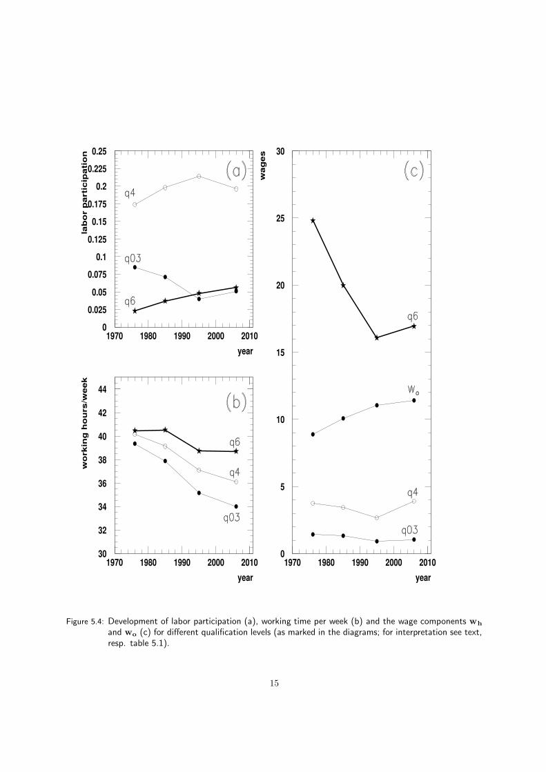
The above redistribution phenomena are further investigated. The sample of employed workers isdivided up in 4 groups of qualification: low (q03-group), medium (q4-group), high (q5-group) and highest(q6-group) qualification (see table 5.1). (The inclusion of self-employed would result only in a minorcorrection because their number is only ≈ 10% of the employed and the wages of the q-groups areidentical.) For the 4 qualification groups the parameters of labor participation, weekly working hours,and wage-components are determined. They are shown in figure 5.4 for the different years; table 5.6shows the detailed numbers.

At first the amount of labor is considered, using labor participation and working time per week:

• over the full time range the general labor participation rises by +8% (fig. 5.4 (a)), while the weeklyworking hours decrease by -9% (fig. 5.4 (b)). So the amount of labor per person has practicallynot changed in the 30 years including the unification.

• the labor participation of the q6-group shows a remarkable and nearly constant growth of +140%over the full time range (fig. 5.4 (c)).

These facts demonstrate a considerable increase of the qualification of the labor force: the highest quali-fication group shows a very high increase going along with the decrease of jobs for the low-q group. Sothe productively used H should have increased accordingly.

However, the surplus wage for the productively used H, wh, has decreased: by 32%, up to 1996 even by35%. In the last period an increase to 16.1Euro/h (by 14%) is visible. This is a considerable re-increase,however, still far from the original level of 21.1Euro/h.

Further on the group of low qualification q03 has realized a loss of -40% in the labor participationand of -14% in the weekly working hours. This loss of more than 50% of the labor demand for this grouphas resulted in the well known high rate of long time unemployment of low qualified workers. So thenon-existence of a sufficient demand for this type of labor has to be stated.

10

Contrariwise the income share of capital has increased by 64%, in the last period alone by 48%. Sothe increase in qualification is either not properly honored by the employers, or the higher qualified pushthe lower qualified out of their jobs: accepting jobs of lower qualification level and lower wage. Whateverthe reasons are, in the end there are much more jobs for the highest qualification level and a loss of about50% of low qualification jobs.

The consequences of these facts are:

• the loss of more than 50% of low qualified labor demand resulted in a high unemployment and adecrease of the basic wage wo as compared to the general trend of growth,

• the q6-group has compensated the loss in labor participation,

• the wage of the q6-group is still quite low as compared to the earliest data. Their probably incom-plete representation by trade unions does not allow them to enforce sufficient higher wages.

• as a consequence the employers profit from this situation: Their income share has increased by65%.

5 Discussion of the Results for Germany

The method has been applied to German data of the years 1976, 1985, 1995, 2006. The German MZ-data of these years have been used to obtain W and wo of EL and SE. Data of the German “Volk-swirtschaftliche Gesamtrechnung” (VGR) of the Statistisches Bundesamt are then evaluated to obtainthe real total income shares of the production factors of physical and human capital and labor. Theaverage shares (1976 - 2006) for Germany yield

sK : sHp: sLo

= 0.18 : 0.26 : 0.56. (5.23)

These numbers differ considerably from the generally assumed equal shares of 1/3. It is caused by theseparation of the self-employed labor from the original capital share of the VGR. Without this separation

sK : sHp: sLo

= 0.31 : 0.21 : 0.48 (5.24)

is obtained. This is in agreement with the published results of Mankiw, Romer and Weil and Acemoglu:

sK : sHp: sLo

= 0.30 : 0.28 : 0.42 98 countries (1960-1985) [8] (5.25)

= 0.36 : 0.26 : 0.38 107 countries (1960-2000) [1] (5.26)

The difference to the German data can be attributed to the different model, more stringent assumptionsand the evaluation of about 100 different countries.

The German factor shares of equation 5.23 demonstrate their relative importance for the growthof the country. Remarkable is the considerably higher share of H w.r.t. K. The very high value of sL

demonstrates the importance of technology which contributes to this share in form of technology enhancedwages.

The development of the income shares from 1976 to 2006 does not show a constant behavior asexpected from Kaldor’s stylized fact for developed countries. It could apply to the human capital share.But definitely not to the shares of capital and labor. Instead there is a sudden increase of the capitalshare in the period from 1995 to 2006 by 0.080, a 48% change. The labor share decreases accordingly.This is in complete contradiction with an expected constant behavior.

An explanation for this feature can be a strong structural change. Evidence is coming from a moredetailed analysis of MZ data: the development of parameters like labor participation and wages from

11

human capital for groups of different qualification. Over the whole 30-years period an enormous shift ofqualification towards a higher level is encountered. This fact manifests in a 140% increase of the group ofhighest qualification (degree of university or “Fachhochschule”). This goes along with a constant overallwork participation while workers with low qualification suffer from a 50% loss of jobs.

However, the highest qualified workers did not profit from this development. Instead the surplus wageof productively used H decreased by more than 30% in spite of a growth of GDP and total income bynearly 30%. As a result the employers have profited much more than the qualified workers by an increaseof their income share by about 65%.

In sum there is the positive effect of the large increase of workers with highest qualification, which iscertainly an increase of the productively used H. But it does not show up in sH because of a decreasingwage for the productive H. This highly questionable effect is certainly no incentive for investments inhigher education. Therefore this fact should be transmitted to government and/or the employers withthe request for a change.

The markable changes of income shares within the last 10 years, and its probable origin, the strongstructural changes, opens a box of new questions:

• to government: how to handle and overcome the resulting unwanted consequences

• to growth theory: how to implement effects like the IT-revolution, or globalization effects.

• to economic science: is there a method to identify the origin and estimate its effect on economyand population, and are there early indicators?

At present there are no answers to these questions. They can be addressed in future investigations thatwould involve more detailed analysis of micro data as well as detailed time series with yearly frequency.of e.g. the income shares, labor participation, etc.

Finally the results for Germany should be compared to those of other countries, e.g. in Europe. Theanalysis of differences and similarities might improve the understanding of different developments.

12

6

8

10

12

14

16

18

20

1970 1980 1990 2000 2010year

wag

e/h

0.5

0.55

0.6

0.65

0.7

0.75

0.8

1970 1980 1990 2000 2010year

Figure 5.1: Wages from different methods: W, wo (a) and fo (b).Methods: m1: standard mean (full circle), m2: log-mean (open circle), m3: 10-90 percentiles,linear mean (full square), m4: 10-90 percentiles, log mean (open square), m5: median (star)

024

68

10

1214

161820

1970 1980 1990 2000 2010year

wag

e / h

0.2

0.3

0.4

0.5

0.6

0.7

0.8

1970 1980 1990 2000 2010year

Figure 5.2: Wages (a) and wage fractions (b) of employed (EL) and self-employed (SE) for the years 1976,1985, 1995 and 2006

13

0

0.1

0.2

0.3

0.4

0.5

0.6

0.7

0.8

0.9

1

1970 1975 1980 1985 1990 1995 2000 2005 2010year

real

fact

or s

hare

s(to

tal i

ncom

e)

Figure 5.3: Total income shares of basic labor (sL), human capital (sH), the sum (sL + sH) and physicalcapital (sK) for the years 1976, 1985, 1995 and 2006. Also shown is the labor share as providedby the VGR: sL(VGR) = sL(EL) + sH(EL).

14

00.025

0.05

0.0750.1

0.125

0.150.175

0.20.225

0.25

1970 1980 1990 2000 2010year

lab

or

par

tici

pat

ion

30

32

34

36

38

40

42

44

1970 1980 1990 2000 2010year

wo

rkin

g h

ou

rs/w

eek

0

5

10

15

20

25

30

1970 1980 1990 2000 2010year

wag

es

Figure 5.4: Development of labor participation (a), working time per week (b) and the wage components wh

and wo (c) for different qualification levels (as marked in the diagrams; for interpretation see text,resp. table 5.1).

15

Level Qualification persons wage/hour [Euro][1000]

in 2006 1976 1985 1995 2006q0 w/o qualification 482 11.5q1 basic schooling finished 1820 9.6 10.8 11.9 12.5q2 higher schooling finished 1526 13.4 12.0 11.1 12.5q3 learning by doing education 360 13.5 15.5 14.7 13.6q4 apprenticeship 16109 12.6 13.5 13.7 15.3q5 technician, “Meister” 1899 18.7 20.8 19.5 20.0q6 degree of university or “Fachhochschule 4612 33.6 29.9 27.1 28.4

Table 5.1: Unified levels of qualification, professional training, frequencies (2006-data), and wage per hour indifferent years. Wages are corrected for inflation and converted to Euro. The wages of minimalqualification q0 is included in q1 for the years 1976 - 1995.

year 1976. 1985. 1995. 2006.wage/hour [Euro]

W 12.9 14.7 15.2 17.0wo 8.9 10.1 11.0 11.4wh 4.0 4.6 4.2 5.6fo 0.686 0.684 0.723 0.670fh 0.314 0.316 0.277 0.330

Table 5.2: Wages and fractions of basic wage and human capital of the employed workers. Results are correctedfor inflation and converted to Euro.

year 1976. 1985. 1995. 2006.wage/hour [Euro]

W 15.1 17.3 17.5 18.9wo 8.9 10.1 11.0 11.4wh 6.2 7.2 6.5 7.5fo 0.590 0.581 0.629 0.605fh 0.410 0.419 0.371 0.395

Table 5.3: Wages and fractions of basic wage and human capital of the self-employed. Wages are correctedfor inflation and converted to Euro.

16

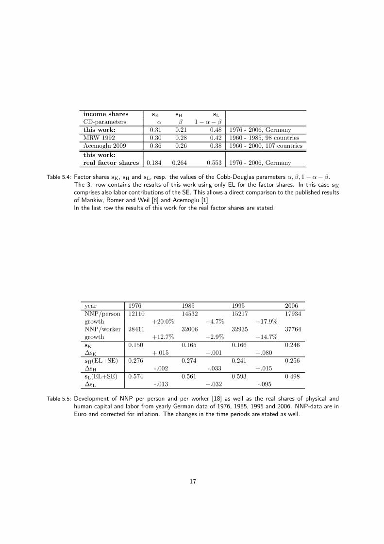
income shares sK sH sL

CD-parameters α β 1 − α − βthis work: 0.31 0.21 0.48 1976 - 2006, GermanyMRW 1992 0.30 0.28 0.42 1960 - 1985, 98 countriesAcemoglu 2009 0.36 0.26 0.38 1960 - 2000, 107 countries

this work:real factor shares 0.184 0.264 0.553 1976 - 2006, Germany

Table 5.4: Factor shares sK, sH and sL, resp. the values of the Cobb-Douglas parameters α, β, 1 − α − β.The 3. row contains the results of this work using only EL for the factor shares. In this case sK

comprises also labor contributions of the SE. This allows a direct comparison to the published resultsof Mankiw, Romer and Weil [8] and Acemoglu [1].In the last row the results of this work for the real factor shares are stated.

year 1976 1985 1995 2006NNP/person 12110 14532 15217 17934growth +20.0% +4.7% +17.9%NNP/worker 28411 32006 32935 37764growth +12.7% +2.9% +14.7%sK 0.150 0.165 0.166 0.246∆sK +.015 +.001 +.080sH(EL+SE) 0.276 0.274 0.241 0.256∆sH -.002 -.033 +.015sL(EL+SE) 0.574 0.561 0.593 0.498∆sL -.013 +.032 -.095

Table 5.5: Development of NNP per person and per worker [18] as well as the real shares of physical andhuman capital and labor from yearly German data of 1976, 1985, 1995 and 2006. NNP-data are inEuro and corrected for inflation. The changes in the time periods are stated as well.

17

year 1976. 1985. 1995. 2006. change[%]

mean labor participation 0.301 0.330 0.327 0.326 8.3

[workers/population]mean working time 40.0 39.1 37.2 36.3 -9.3

[h/week]W 12.9 14.7 15.3 17.0 31.6wo 8.9 10.1 11.0 11.4 28.4wh 4.1 4.6 4.2 5.6 38.7labor participationq03 0.085 0.071 0.040 0.051 -40.1q4 0.174 0.198 0.214 0.196 12.3q5 0.018 0.024 0.025 0.023 27.1q6 0.023 0.037 0.048 0.056 139.9working timeq03 39.4 37.9 35.2 34.0 -13.6q4 40.2 39.1 37.1 36.1 -10.1q5 41.0 40.4 38.5 37.7 -8.1q6 40.5 40.5 38.7 38.7 -4.3wh

q03 1.4 1.3 0.9 1.0 -26.2q4 3.8 3.4 2.7 3.9 3.8q5 9.8 10.8 8.5 8.6 -12.9q6 24.8 20.0 16.1 16.9 -31.7

Table 5.6: Developments of parameters for groups of different qualification: from low (q03) to the highest (q6)level (see text for further explanation). The last column contains the total change from 1976 to2006.

18

A Appendix

A.1 GDP and Total Income

GDP and total income are closely related. For Germany both are determined by the “StatistischesBundesamt” in the yearly VGR (“Volkswirtschaftliche Gesamtrechnung”) [14]. The relation is given by

GDP 100% (2006)± net factor income from abroad +2.0%- depreciation -14.5%± indirect taxes(-) und subsidies(+) - 9.6%= NNP ≡ total income 78.2%

= sL(VGR): employed labor income share 63.9% (NNP)+ sK(VGR): self-employed and firms income shares 36.1% (NNP)

The NNP (net national product) is the total income of the economy. Its difference to the GDP israther constant being ≈ 22%: the variation in time from 1970 - 2011 is less than ±0.5%. It is the basisfor the annual income shares of capital and labor. The VGR separates the NNP into the labor incomeshare sL(VGR) comprising only the labor income of employed workers, and the capital share sK(VGR)comprising the income share of enterprises as well as investment and labor share of self-employed workers.

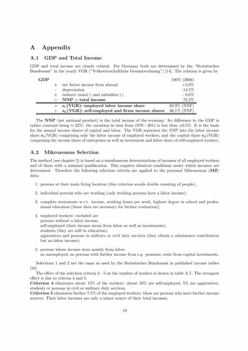
A.2 Mikrozensus Selection

The method (see chapter 2) is based on a simultaneous determinations of incomes of all employed workersand of those with a minimal qualification. This requires identical conditions under which incomes aredetermined. Therefore the following selection criteria are applied to the personal Mikrozensus (MZ)data:

1. persons at their main living location (this criterion avoids double counting of people),

2. individual persons who are working (only working persons have a labor income);

3. complete statements w.r.t. income, working hours per week, highest degree in school and profes-sional education (these data are necessary for further evaluation);

4. employed workers: excluded arepersons without a labor income,self-employed (their income stems from labor as well as investments),students (they are still in education),apprentices and persons in military or civil duty services (they obtain a subsistence contributionbut no labor income);

5. persons whose income stem mainly from labor:no unemployed, no persons with further income from e.g. pensions, rents from capital investments.

Selections 1 and 2 are the same as used by the Statistisches Bundesamt in published income tables[10].

The effect of the selection criteria 3 - 5 on the number of workers is shown in table A.7. The strongesteffect is due to criteria 4 and 5.Criterion 4 eliminates about 15% of the workers: about 10% are self-employed, 5% are apprentices,students or persons in civil or military duty services.Criterion 5 eliminates further 7.5% of the employed workers: these are persons who have further incomesources. Their labor incomes are only a minor source of their total incomes.

19

In total the selection criteria eliminate 23.5% of the working population. However, the remaining 76.5%comprise the essential fraction of the labor incomes of the employed workers.

It should be noted that for the later estimation of the labor income of the self-employed (chapter 3.2)the criterion 4 is changed accordingly.

A.3 Details of Income Conversions

Income scale: The income is stated in the MZ data as net monthly income. These statements aregiven in an ordinal scale that differs for different years. For the 2006-data it is

{< 150,−300,−500,−700,−900, ...,−7500,−18000, > 18000} Euro.

The lowest and the highest bins are unlimited. They have been converted to confined bins by fixing therange to 50 < income < 28000. Income values outside the range are changed to the minimal/maximalvalue. The lower bound has practical reasons: it allows the evaluation of logarithmic distributions. Theupper bound limits extreme incomes in order to reduce their influence on a mean.

Income distributions are evaluated in using the bin centers of the ordinal scale.

Gross income: The net income has to be converted into gross income. This is necessary for a laterconversion of wage ratios into shares of the total income which is the sum of gross incomes.

The difference between gross and net income comprises income tax, social insurances and contributionsof employers. The conversion of net to gross income is performed by determining the conversion for thedifferent bounds of the ordinal scale. In detail the following procedure is used:

1. the income is multiplied by 12 in order to obtain the yearly income,

2. the income tax is calculated using the tax law of the different years [2],

3. contributions to social insurance as well as contributions to it from employers are obtained fromthe VGR-tables [19] of the different years,

4. the resulting gross income is divided by 12 in order to obtain the gross monthly income.

The resulting gross scale is used for the evaluation of the income distribution.

Inflation correction: Incomes of different years can be compared only if corrections for inflationare applied. The different deflaters are determined from the tables of nominal and deflated GDP valuesof the years [18]. For Germany there are 2 different tables for the time before and after the unification.They overlap for the year 1991. Therefore 1991 is used as reference year. The obtained deflaters arelisted in table A.10.

Income per hour: The weekly working hours have changed with the years. In addition the tendencyto work part time has increased. Therefore the monthly income is converted to income per hour by usingthe MZ statements on the weekly working hours and assuming 4 weeks per month. The final distributionof income per hour has equidistant bins with the overflow accumulated in the last bin.

Conversion to Euro: The incomes obtained so far are stated in different units: DM and Euro.All DM-values are converted to Euro using the ratio Euro/DM = 1.95583.

20

A.4 The Unified Scale of Qualification Levels

When investigating incomes of workers of different qualification a scale of qualification has to be defined.This scale has to be the same for all years.

In the Microzensus data the educational and professional qualification is stated separately as highestdegree reached in schooling as well as in professional qualification. As a consequence all persons arecounted twice in the 2 qualification scales. For the 2006-data the different degrees are listed in table A.8.There are 6 levels for schooling and 11 levels for professional qualification (university and “Fachhochschul”degrees are listed as professional qualification; schooling degree of “Abitur” or “Fachhochschulreife” areindispensable for them).

Figure A.5 shows the frequency (a) as well as the average net monthly income (b) for different qual-ifications. The income distribution (b) shows 2 independent qualifications scales: schooling (0 - 6) andprofessional degree (10 -20). For either scale the income rises with increasing qualification. They have tobe combined to a single scale without any double counting. This unified scale which is valid for all yearsis obtained after the following procedure:

• the degrees of the former GDR are combined with appropriate degrees of the German federalrepublic,

• the professional qualification is given priority over the schooling qualification: it shows a strongerdynamic with the professional degree and minimal schooling degrees are indispensable for the higherprofessional degrees,

• qualifications with too few persons have been combined in order to avoid qualification groups withtoo low population.

The final qualification scale is shown in table A.9. 7 different groups (q0 - q6) are specified togetherwith the relative population. The also stated net monthly income shows a considerable increase with thequalification level.Further on combined groups are specified: the low qualification group q03 comprises q0 - q3, and thegroup q01 comprising q0 and q1.

The group q01 has been formed in order to overcome a problem of the data from 1976 - 1995. In thesedata there is no differentiation between q0 and q1. However in the 2006-data q0 and q1 are separatequalification groups that show an income difference of 7%. This difference is used to obtain wo = w(q0)for all years:

wo = w(q01) ·W(q0)2006W(q01)2006

.

A.5 wo Determination

wo is determined as income of workers with minimal qualification. In Germany these are persons whohave passed the obligatory years of schooling (about 8). But they finished schooling without a degree.

As shown in equation 2.1 a Harrods neutral technology is involved that results in a technology enhancedwage. The technology is country specific, in this case specific for Germany.

In addition also wh, the surplus income from H engagement, might include effects of current tech-nology. This has to be taken into account in comparisons of wo and wh or of income shares of differentcountries.

An alternative determination of wo is the result of a Mincer regression [11]:

ln w = α + ρ · s + βox + β1x2 + ε,

with the variable s (number of school years) and x (years of working). The value of α, obtained from theregression, is assumed to be the logarithm of the wage for a worker with 0 years of schooling. Argumentsagainst this method are:

21

1. in many developed countries there are no persons without any schooling; therefore one has to relyon the linearity of the above Mincer equation.

2. the type of schools differ considerably; therefore the parameter ρ and with it the extrapolation to0 school years is determined by the population of the different types of schools,

3. the German MZ data do not contain statements about the years of schooling; there are only state-ments on the highest degree reached. An estimate of the years of schooling is not excluded, but ithas not been investigated.

Further on the linearity requirement would be an additional rather strong assumption. This is avoidedby using the wage of workers with minimal qualification.

A.6 Wage Determination from Income Distributions

The two wages W and wo are determined from income distributions of two groups: the incomes of allemployed (W) and the incomes of workers with minimal qualification (wo). However, the distributionsof the two groups differ considerably as shown in figure A.6 with linear (left: a,c) and log. (right: b,d)income scales.

Comparing the linear distributions one observes a long tail of the W-distribution (a). This is absentin the wo-distribution (c). This fact will result in a mean that is systematically biased by the extremehigh values of the W-distribution. This is also a potential source of a higher volatility of this value indifferent years. The logarithmic distributions show the reverse effect: a stronger tail to the low side ofthe wo-distribution.

Both effects introduce a bias of the important wage ratios fo and fh. Therefore different methodshave been studied in order to determine representative values of W and wo from the linear and thelogarithmic distributions. The difference of the results between linear and logarithmic distributions (∆)will be a kind of measure for the sensitivity to the tails of the distributions: to the low side (log) or thehigh side (linear).

The following methods have been evaluated: the standard mean using the full distributions, themean of the 10-90-percentiles of the distributions, and the median (the median is identical for linearand logarithmic distribution). The results are shown in table A.11 for 4 years from 1976 to 2006. Theimportant number in this table is ∆. It demonstrates the effect of high and low tails.

The standard means yield rather large differences ∆: ≈20% of the mean. However, the wage ratio foshows only small differences. This originates from the tails of the distributions:linear distribution: systematic larger value for W and normal value for wo;logarithmic distribution: systematic lower value for wo and normal value for W;For the wage ratio fo = wo / W the systematic effects go into the same direction yielding small differences.But the value of fo itself is systematically low.

The means from the 10-90-percentile distribution yield smaller values of ∆: ≈7% of the mean. Thewage ratio fo shows negligible differences. This results from the absence of high and low tails in the10-90-percentile distributions.

The median values are the same for linear and logarithmic distributions: ∆ = 0.0. However the valuesshow a stronger fluctuation over the years as compared to the other methods. This is esp. visible for fo,shown in figure 5.1 (b). In this figure fo(median) fluctuates considerably up and down from 1976 - 2006;the other fo-values show a nearly linear rise up to 1995 and a sharp fall in the last period. A reason forthe fo-behavior of the median is the ordinal scale of the income distributions. A too coarse binning inthe range of the median value results in larger fluctuations as compared to average values.

The finally accepted method for the determination of W and wo is the mean of the 10-90-percentilelinear distributions:it has a low dependence on tails to the high or low side (as compared to the standard mean),

22

it is less sensitive to the binning of the income distribution (as compared to the median),it is preferable to the evaluation of the logarithmic distributions, if subsamples (like groups of differentqualification level) are analyzed: the weighted means of the subsamples do not add up to the total meanin case of a logarithmic distributions.

23

Figure A.5: Frequency (top) and net monthly income (bottom) of different qualification levels from schooland professional education. The numbers of the horizontal scale refer qualification groups of tableA.8. The number 0 refers to persons having neither a degree from schooling nor from professionaltraining. The number 24 refers to the overall average.

24

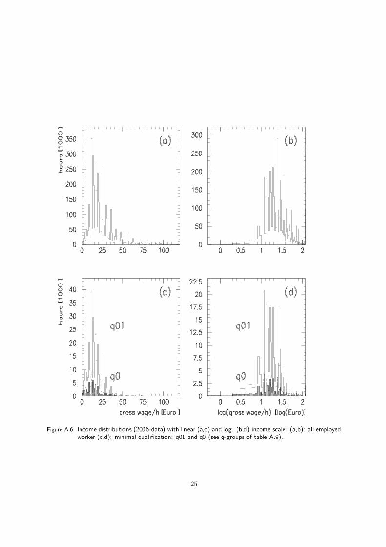
Figure A.6: Income distributions (2006-data) with linear (a,c) and log. (b,d) income scale: (a,b): all employedworker (c,d): minimal qualification: q01 and q0 (see q-groups of table A.9).

25

Selection Persons Selected[1000] Fraction

1 + 2 : preselection 35 063 100%3. complete statements 34 596 98.74. employed 29 436 84.05. mainly labor income 26 812 76.5

Table A.7: Results for Selections 3 - 5 (2006-data)

code schooling degree code professional degree1. no schooling level 10. no professional level2. basic school 11. learning-by-doing training3. “Polytech.Oberschule: DDR” 12. “Berufsvorbereitungsjahr”4. “Realschule” 13. apprenticeship5. “Fachhochschulreife” 14. “Berufsfach-, Kollegschule”6. “Abitur” 15. technician, “Meister”

16. ”Fachschule der DDR”17. ”Verwaltungs-Fachhochschule”18. ”Fachhochschule”19. university20. PhD

Table A.8: Qualification groups of 2006 data: highest degree obtained in education and professional training.The codes refer to the horizontal scale in figure A.5 showing population and net income of thegroups.

level qualification persons income[1000] [Euro/h]

in 2006q0 w/o qualification level 482 14.0q1 no prof.level, basic school degree 1820 15.3q2 no prof.level, higher school degree 1526 15.3q3 learning-by-doing training 360 16.6q4 apprenticeship 16109 18.7q5 technician, “Meister” 1899 24.5q6 university or ”Fachhochschule” degree 4612 34.7q03 low qualified: levels q0 - q3 4188 15.3q01 min.qualification: q0 - q1 2302 15.0

Table A.9: Unified qualification levels, population and net monthly income of 2006 data. For q3 - q6 no schooldegrees are required explicitly, but there are implicit requirements.

Jahr 1976 1985 1995 2006

Deflater 1.593 1.163 0.873 0.817

Table A.10: Inflation correction for the years 1976 - 2006..

26

method distr. variable 1976 1985 1996 2006standard mean linear W 15.6 16.9 17.1 19.2

log. W 12.4 13.9 14.3 15.8∆ 3.2 3.0 2.8 3.4

linear wo 9.6 10.8 11.6 12.4log. wo 8.0 9.1 9.8 9.8

∆ 1.6 1.7 1.8 2.6linear fo 0.61 0.64 0.68 0.64log. fo 0.64 0.65 0.68 0.62

∆ -0.027 -0.014 -0.004 0.023mean of linear W 12.9 14.7 15.3 17.010-90-percentile log. W 12.2 13.8 14.4 15.8

∆ 0.7 0.9 0.9 1.2linear wo 8.9 10.1 11.0 11.4log. wo 8.3 9.5 10.4 10.5

∆ 0.6 0.6 0.7 0.9linear fo 0.69 0.68 0.72 0.67log. fo 0.68 0.69 0.72 0.66

∆ 0.007 -0.003 0.004 0.008median W 12.0 13.3 13.9 15.3

∆ 0.0 0.0 0.0 0.0wo 9.2 9.6 10.6 10.7∆ 0.0 0.0 0.0 0.0fo 0.77 0.72 0.76 0.70∆ 0.0 0.0 0.0 0.0

Table A.11: Results of different methods for mean income of all employed workers and those with minimalqualification and the wage ratio fo. Results from linear and logarithmic distributions as well as thedifference ∆.

27

References

[1] D. Acemoglu: “Introduction to Modern Economic Growth”, S. 93, Princeton University Press,Princeton, NJ, USA, 2009.

[2] Einkommensteuergesetz v. 19.10.2002 (BGBl I S. 4212, ber. 2003 I S. 179), §32a: Einkommensteuer-tarif.Eine Ubersicht der Steuertarife in den Jahren 1958 - 2005 des Bundesministeriums fur Finanzen findetman auf dem Internet: “http://steuervereinfachung.snrk.de/TarifgeschichteoF.pdf”, 11.4.2012.

[3] Folloni, Giuseppe; Vittadini, Giorgio; “Human Capital Measurement: A Survey” Journal of Eco-nomic Surveys, April 2010, v. 24, iss. 2, pp. 248-279

[4] Jeong, B.: “Measurement of human capital input across countries: a method based on the laborer’sincome” Journal of Development Economics Vol. 67, 333-349, 2002.

[5] Kaldor, Nicholas (1961): “Capital Accumulation and Economic Growth” in The Theory of Capital,Hrsg. F.A.Lutz and D.C.Hague, New York: St. Martins

[6] Koman, Reinhard; Marin, Dalia: “Human Capital and Macroeconomic Growth: Austria and Ger-many 1960-1997, an update” Institute for Advanced Studies, Economics Series: 69, 1999.

[7] Le,T.; Gibson, J.; Oxley, L.: “Cost and income based measures of human capital”. Journal ofEconomic Surveys 17(3), 271-305, 2003.

[8] Mankiw, N. Gregory, Romer, David, Weil, David (1992): “A Contribution to the Empirics of Eco-nomic Growth”, Quarterly Journal of Economics, 107, 407 - 438

[9] Mikrozensus details of topics and questions of annual interviews are available from the internet:http://www.gesis.org/unser-angebot/daten-analysieren/amtliche-mikrodaten/mikrozensus/grundfile/

[10] Mikrozensus 2006: Fachserie 1 Reihe 4.1.2 “Bevolkerung und Erwerbstatigkeit, Beruf, Ausbildungund Arbeitsbedingungen der Erwerbstatigen, Band 2: Deutschland”, Tabelle 2.1: ”Erwerbstatigemit Angabe des monatlichen Nettoeinkommens nach allgemeinem Schulabschluss, beruflichemAusbildungs- bzw Hochschulabschluss und monatlichem Nettoeinkommen”, Statistisches Bunde-samt, Wiesbaden, Germany, March 2008https://www.destatis.de/DE/Publikationen/Thematisch/Arbeitsmarkt/ Erwerbstaetige/ BerufAr-beitsbedingungErwerbstaetigenBandII2010412067424.pdf (27.4.2008, 18:30)

[11] Mincer, J.: “Investment in Human Capital and Personal Income Distribution” Journal of PoliticalEconomy 66(4), 281-302, 1958.

[12] Mulligan, C. B.; Sala-i-Martin, X.: “A Labor-Income-Based Measure of the Value of Human Capital:an Application to the States of the United States” Japan and the World Economy, May 1997, v. 9,iss. 2, pp. 159-91

[13] OECD-Report; “Human Capital Investment. An International Comparison”. Paris: Center for In-ternational Research and Innovation, 1998

[14] Statistisches Bundesamt, Fachserie 18, Reihe 1.4 “Volkswirtschaftliche Gesamtrechnungen, Inland-sproduktberechnung, Detaillierte Jahresergebnisse”, Wiesbaden, 2011.https://www.destatis.de/DE/Publikationen/Thematisch/VolkswirtschaftlicheGesamtrechnungen/Inlandsprodukt/InlandsproduktsberechnungEndgueltig2180140107004.htmlTabelle 3.1.1: Wertschopfung,Inlandsprodukt und Einkommen.

[15] ibid. Tabelle 3.1.2: Wertschopfung,Inlandsprodukt und Einkommen, row 30

28

[16] Statistisches Bundesamt, Fachserie 18, Reihe 1.5: “Volkswirtschaftliche Gesamtrechnungen, Inlans-dsproduktberechnung, Lange Reihen ab 1970”, Wiesbaden, 2011.https://www.destatis.de/DE/Publikationen/Thematisch/VolkswirtschaftlicheGesamtrechnungen/Inlandsprodukt/InlandsproduktsberechnungLangeReihenPDF 2180150.html

[17] ibid. Tabelle 1.3: Volkseinkommen und verfugbares Einkommen der Volkswirtschaft, Wiesbaden,2011

[18] ibid. Tabelle 1.4: Bruttoinlandsprodukt, Bruttonationaleinkommen, Volkseinkommen (Pro-Kopf-Angaben), Wiesbaden, 2011

[19] ibid. Tabelle 1.8: Sozialbeitrage der Arbeitgeber und Arbeitnehmer, Wiesbaden, 2011

29