THE REDUCED FORM: A SIMPLE APPROACH TO INFERENCE WITH

WEAK INSTRUMENTS

VICTOR CHERNOZHUKOV AND CHRISTIAN HANSEN†

Abstract. In this paper, we consider simple and practical methods for performing het-

eroskedasticity and autocorrelation consistent inference in linear instrumental variables mod-

els with weak instruments. We show that conventional inference procedures based on the

reduced form about the relevance of the instruments excluded from the structural equation

lead to tests of the structural parameters which are valid even if the instruments are weakly

correlated to the endogenous variables. The use of standard heteroskedasticity and autocor-

relation consistent covariance matrix estimators in constructing these tests also results in

inference which is robust to heteroskedasticity, autocorrelation, and weak instruments. We

extend the basic results for the linear instrumental variables model to provide an approach

to inference for quantile instrumental variables models which will be valid under weak iden-

tification. We provide a simulation experiment that demonstrates that the procedures have

the correct size and good power in many relevant situations and conclude with an empirical

example.

Keywords: quantile regression, weak instruments, heteroskedasticity, autocorrelation

1. Introduction

In many applied economics papers, interest focuses on identification and estimation of

coefficients on endogenous variables in linear structural equations with mean or quantile

independence restrictions. The identification of these coefficients is made possible by the use

of instrumental variables that are assumed to be correlated to the right hand side endogenous

variables but uncorrelated with the structural error. When the instruments are strong, there

are many estimation and inference procedures, such as 2SLS and LIML, that can be used to

estimate the parameters and obtain asymptotically valid inference statements.

Date: 20 January 2005. First draft: 10 August 2004. We thank Josh Angrist, Alan Bester, Jon Guryan,

Byron Lutz, and Josh Rauh for useful comments and discussion.†University of Chicago, Graduate School of Business, 5807 S. Woodlawn Ave., Chicago, IL 60637. Email:

chansen1@gsb.uchicago.edu.1

However, when the instruments are weak, that is when the correlation between the en-

dogenous variables and instruments is low, conventional asymptotics may provide poor ap-

proximations to the finite sample distributions of conventional estimators and test statistics.

This breakdown in the asymptotic approximation may lead to highly misleading inference

about the parameters of interest.

The potential poor performance of conventional inference procedures in the presence of

weak instruments has led to the development of a number of inference procedures that remain

valid in the presence of weak instruments. For the linear IV model with homoskedastic

errors, Anderson and Rubin (1949) (hereafter AR) introduced a statistic based on the LIML

likelihood which is valid under weak identification. This statistic has been further analyzed

by Zivot, Startz, and Nelson (1998), Dufour and Jasiac (2001), and Dufour and Taamouti

(2005) who provide closed form solutions for computing confidence sets, though the results

of these papers do not apply to the more general case of when the structural errors may be

heteroskedastic or autocorrelated. Stock and Wright (2000) proposed the S statistic which

generalizes the AR statistic to the general GMM setting and allows for heteroskedasticity

and autocorrelation.

The chief drawback of the AR and S statistics is that they may have low power when there

are many more instruments than endogenous variables. To overcome this problem, Moreira

(2003) proposed a likelihood ratio based statistic and Kleibergen (2002) proposed a Lagrange

multiplier type statistic both of which are robust to weak instruments in the homoskedastic

error case and tend to have more power in models with more instruments than endogenous

regressors. Kleibergen (2004, 2005) generalizes Kleibergen’s (2002) approach to the general

GMM setting and allows for heteroskedasticity and autocorrelation. Similary, Andrews,

Moreira, and Stock (2004a, 2004b) generalize Moreira’s (2003) conditional likelihood ratio

statistic to allow for heteroskedasticity and autocorrelation and show that this statistic is

optimal among a class of invariant similar tests. For excellent surveys of these and other

results and a more detailed discussion of the weak instrument problem, see Stock, Wright,

and Yogo (2002) and Andrews and Stock (2005).

In this paper, we consider a simple and practical approach to performing inference that will

be valid under weak identification. We demonstrate that the approach results in tests with

the correct size in the presence of weak instruments and that the tests can be made robust

2

to heteroskedasticity and autocorrelation through the use of conventional robust covariance

matrix estimators. The simplest version of the procedure we propose may be viewed as a

simple and intuitive approximation to the S-statistic of Stock and Wright (2000) in that the

approaches are asymptotically equivalent regardless of the strength of the instruments. The

procedure can also be made asymptotically equivalent to the LM approaches of Kleibergen

(2002, 2004, 2005) through appropriate choice of instruments. In addition, the number

of excluded instruments equals the number of right hand side endogenous variables in the

majority of IV studies; and in this case, the approaches of Stock and Wright (2000), Moreira

(2003), and Kleibergen (2002) are equivalent and share the optimality properties discussed in

Andrews, Moreira, and Stock (2004b). Thus, our procedure will be asymptotically optimal

in this empirically relevant case.

The most appealing feature of the procedure is that it relies only on OLS estimation and

inference and so may be easily implemented using standard inference tools available in almost

any regression software. In particular, in the simplest case, weak-instrument robust proce-

dures that are also robust to heteroskedasticity or autocorrelation for testing the hypothesis

that β = β0 may easily be constructed through linear regression of a transformed dependent

variable, Y −Xβ0, on the set of instruments, Z, where X is the set of endogenous variables

and testing that the coefficients on Z are equal to 0 using a conventional robust covariance

matrix estimator. Angrist and Krueger (2001) have also recommended this approach in the

special case of testing the hypothesis that β = 0 when one is worried that identification may

be weak.

In addition to this basic procedure, we consider two important extensions. First, using

the intuition of Kleibergen (2002, 2004, 2005), we show how the set of instruments may be

collapsed to the dimension of the endogenous regressors in settings where there are more

instruments than endogenous regressors in a way that preserves validity under weak identi-

fication and results in power gains relative to the unmodified procedure. Second, we show

how the basic principle may be adapted to obtain tests and confidence intervals that will

be valid under weak identification for the instrumental variable quantile regression (IVQR)

estimator of Chernozhukov and Hansen (2004) which estimates quantile treatment effects

under endogeneity.

3

We illustrate that the tests have good size and power properties in a simulation study.

To provide some motivation for the simulation design, we report results from a survey of IV

papers published in leading applied journals from 1999 to 2004. We also provide an empirical

example which illustrates the practical importance of accounting for weak instruments.

The remainder of this paper is organized as follows. In the next section we outline the basic

testing procedure. In Section 3, we show how this basic procedure may be adapted to obtain

more powerful tests in cases where there are more instruments than endogenous regressors

and how the procedure may be adapted to obtain valid confidence intervals and tests for the

IVQR estimator of Chernozhukov and Hansen (2004) under weak identification. Section 4

then discusses the simulation example, and Section 5 contains an empirical application. We

conclude in Section 6.

Throughout the paper we make use of the following notation: For an n× k matrix A with

columns a1, . . . , ak, vec(A) = (a′1, . . . , a

′k)

′, PA = A(A′A)−1A′ and MA = In − PA where In

denotes an n×n identity matrix. In addition, we will refer to a model as being just-identified

if the order condition for identification is satisfied with equality, that is if there are exactly as

many instruments as endogenous variables. We will refer to a model as being overidentified

when there are more instruments than endogenous variables.1

2. Model Specification and Testing Procedure

2.1. Basic Specification and Intuition. Suppose we are interested in estimating the pa-

rameters from a structural equation in a simultaneous equation model that can be represented

in limited information form as

Y = Xβ + ǫ (1)

X = ZΠ + V (2)

1Note our use of these terms differs from conventional definitions in linear IV models in that we do not

require the rank condition to be satisfied.4

where Y is an n × 1 vector of outcomes, X is an n × s matrix of endogenous right hand

side (RHS) variables, and Z is an n × r matrix of excluded instruments where r ≥ s.2 The

condition that r ≥ s simply insures that the order condition for identification is satisfied;

i.e. there are, in principle, sufficient instruments to identify the parameters of interest.

The testing procedure we consider may then be motivated in the following manner. Sup-

pose we are interested in testing the null hypothesis that β = 0 versus the alternative that

β 6= 0. When the instruments are highly correlated to X, we can proceed by estimating

β by 2SLS and using this estimate and the corresponding asymptotic distribution to test

the hypothesis. However, when the instruments are weakly correlated with X, the usual

asymptotics may provide a poor approximation to the actual sampling distributions of the

estimator and test statistics. An alternative, “dual”, approach based on the reduced form for

Y is also available. In particular, under the null hypothesis, the exclusion restriction implies

that the coefficients on the instruments in the reduced form for Y , defined by substituting

equation (2) into equation (1) to obtain Y = Zγ + U , should equal zero. Thus, testing that

these coefficients equal 0 tests the hypothesis that β = 0. It is easy to see that this proce-

dure will be robust to weak instruments since in testing that the reduced form coefficients

on the instruments are equal to 0 no information about the correlation between X and Z is

required.

This basic intuition may be extended easily for testing the more general hypothesis that

β = β0. In this case, we may think of writing (1) as

Y − Xβ0 = Zα + ǫ. (3)

2Note that this model allows for additional RHS predetermined or exogenous regressors which have been

“partialed out” of the specification. That is, the above model will accommodate a model defined by

Y = Xβ + Wγ + ǫ

X = ZΠ + WΓ + V

where W is a vector of exogenous or predetermined variables included in the structural equation of interest.

This model may be put into the form given by equations (1) and (2) by defining Y , X , and Z as residuals

from the regression of Y on W , X on W , and Z on W , respectively. It is also important to note that in

most applications, the dimension of X is small, typically 1 or 2, while the dimension of W is large, making

partialing W out important from a computational standpoint in the procedures outlined below.5

Under the null hypothesis, the exclusion restriction implies that α = 0, so a test of α = 0

in equation (3) tests the null that β = β0. Letting WS(β0) denote the conventional Wald

statistic for testing α = 0, we note that the use of a robust covariance matrix estimator, e.g.

a HAC estimator, in forming WS(β0) will result in a robust statistic for testing β = β0 that

will be asymptotically distributed as a χ2r regardless of the strength of the instruments.

Repeating the testing procedure mentioned above for multiple values of β0 also allows the

construction of confidence intervals which are robust to weak instruments and heteroskedas-

ticity or autocorrelation through a series of conventional least squares regressions. The basic

procedure for constructing a confidence interval is as follows:

1. Select a set, B, of potential values for β.

2. For each b ∈ B, construct Y = Y − Xb and regress Y on Z to obtain α. Use

α and the corresponding estimated covariance matrix of α, Var(α), to construct

the conventional Wald statistic for testing α = 0, WS(b) = α′[Var(α)]−1α. Note

that the use of an appropriate robust covariance matrix estimator in forming Var(α)

will result in tests and confidence intervals robust to both weak instruments and

heteroskedasticity and/or autocorrelation.

3. Construct the 1− p level confidence region as the set of b such that WS(b) ≤ c(1− p)

where c(1 − p) is the (1 − p)th percentile of a χ2r distribution.

As with all procedures that are fully robust to weak instruments, the confidence regions

constructed using the procedure outlined above are joint regions for the entire parameter

vector, β. The joint regions are not conservative; however, when s > 1, marginal regions

for the individual components of β obtained through projection methods are likely to be

conservative. It is also worth noting that in overidentified models the test statistic we are

considering provides a joint test of the model specification and the hypothesis that β = β0

and so may result in empty confidence sets in cases where one would reject the hypothesis

of correct specification using the overidentifying restrictions.

2.2. Properties of the “Dual” Inference Procedure. In the previous section, we out-

lined the intuition and basic approach to a “dual” inference procedure for testing hypotheses

about structural parameters that will be valid under weak instruments and can easily be6

made robust to heteroskedasticity and/or autocorrelation. In this section we develop the ba-

sic procedure in more detail and derive the asymptotic properties of the basic test statistics.

Recall from the previous section that for testing the null hypothesis β = β0 versus the

alternative that β 6= β0, we may think of writing equation (1) as

Y − Xβ0 = Zα + ǫ.

Under the null hypothesis, the exclusion restriction implies that α = 0, so a test of α = 0

tests the hypothesis that β = β0.

Considering the homoskedastic case first, a simple test statistic for testing α = 0 is the

standard Wald statistic

WAR(β0) =α′(Z ′Z)α

σ2ǫ

=(Y − Xβ0)

′PZ(Y − Xβ0)1

n−r((Y − Xβ0)′MZ(Y − Xβ0)

, (4)

which is equal to s times the AR statistic. In other words, for testing the hypothesis that

β = β0, the AR statistic may be constructed easily by regressing Y −Xβ0 on Z and testing

that the coefficients on Z are equal to 0. This test bears an obvious close relation to the

standard test of whether the instruments are relevant in the reduced form for Y , where the

reduced form is obtained by substituting (2) into (1) to obtain

Y = Zγ + U. (5)

(3) and (5) are clearly identical when β0 = 0, so the test of instrument relevance in the

reduced form (5) may alternatively be viewed as a weak-instrument robust test of the hy-

pothesis that β = 0.

Similarly, when we drop the assumption of homoskedasticity, a test of α = 0 in (3) may

be constructed from the standard Wald statistic

WS(β0) = α′[Var(α)]−1α, (6)

where Var(α) is a consistent estimator of the variance of α which will generally take the

form (Z ′Z)−1Σn, ǫǫ(ǫ)(Z′Z)−1 for ǫ = Y −Xβ0−Zα and Σn, ǫǫ(ǫ) an estimator of var( 1√

nZ ′ǫ)

evaluated at ǫ. It then follows that WS may be written as

WS(β0) = (Y − Xβ0)′Z[Σn, ǫǫ(ǫ)]

−1Z ′(Y − Xβ0). (7)

7

As above, note that this statistic bears a close resemblance to the S-statistic of Stock and

Wright (2000). In particular, if ǫ were replaced by Y − Xβ0 in WS(β0), WS(β0) would be

identical to Stock and Wright’s S-statistic.

In order to formally discuss testing and obtain the limiting distributions of the test sta-

tistics we propose, we impose the following assumption.

Assumption 1. As n → ∞, the following convergence results hold jointly.

i. 1nZ ′ǫ

p→ 0.

ii. 1nZ ′Z − Mn

p→ 0 where Mn ≡ E[Z ′Z/n] is uniformly positive definite.

iii. Σ−1/2n, ǫǫ

1√nZ ′ǫ

d→ N(0, Ir) where Σn, ǫǫ ≡ var( 1√nZ ′ǫ) with Σn, ǫǫ an r × r matrix.

iv. There is an estimator Σn, ǫǫ(ǫ) that satisfies Σn, ǫǫ(ǫ) −Σn, ǫǫp→ 0 when evaluated at

the true ǫ.

The conditions imposed in Assumption 1 are considerably weaker than those convention-

ally imposed in linear IV models in that they impose no restrictions on the correlation

between Z and X. In other words, Assumption 1 allows for situations in which Z and X are

weakly correlated or even uncorrelated. The last condition in Assumption 1 simply requires

the existence of a consistent covariance matrix estimator. There are numerous examples

of such estimators, such as the Huber-Eicker-White estimator (e.g. White (1980)) in the

heteroskedastic case, a HAC estimator (e.g. Andrews (1991)) for the autocorrelated case, or

a clustered covariance matrix estimator (e.g. Arellano (1987)) in the panel case.

Below, we state the properties of the test statistic WS(β0) under the null hypothesis that

β = β0.

Theorem 1. Suppose that the data are generated by the model defined by (1) and (2), β = β0,

Σn, ǫǫ(ǫ) is uniformly positive definite, and Σn, ǫǫ(ǫ) − Σn, ǫǫ(ǫ) = op(1). If the conditions of

Assumption 1 are satisfied, then

WS(β0) = (Y − Xβ0)′Z[Σn, ǫǫ(ǫ)]

−1Z ′(Y − Xβ0)d→ χ2

r. (8)

Note that the results of Theorem 1 do not require any restriction on the relation between

X and Z. In particular, the results of Theorem 1 will be valid under the three main cases

that have been considered in the literature: (i) The instruments are strong such that Π is8

a fixed, full rank matrix; (ii) the instruments are weak such that Π = C/√

n; and (iii) the

instruments are irrelevant such that Π = 0.

The proof of the theorem is immediate under the condition that Σn, ǫǫ(ǫ)−Σn, ǫǫ(ǫ) = op(1)

since in this case WS(β0) = S(β0)+op(1). The properties then follow immediately from Stock

and Wright (2000). The additional condition will be satisfied for reasonable estimators of

the covariance matrix, such as the Huber-Eicker-White estimator in the heteroskedastic case

and HAC estimators in the autocorrelated case. The condition can be verified by noting

that, under the conditions of Assumption 1, α = Op(1√n) and applying standard arguments;

see, e.g. White (2001).

In cases with dependent data when a HAC estimator is used in estimating the covariance

matrix, a kernel and bandwidth or truncation parameter must also be selected. There

is a large literature on bandwidth selection that could potentially be applied here; see, for

example, Andrews (1991).3 In addition, the results could easily be extended to accommodate

the results about HAC estimation without truncation explored in Kiefer and Vogelsang

(2002). Without truncation, the HAC estimator is not consistent, and the associated Wald

statistic is not a chi-square under the null. However, the Wald statistic does have a well-

defined distribution which does not depend on any unknown parameters and is a functional

of a certain Gaussian process. The critical values for this statistic can easily be obtained

as in Kiefer and Vogelsang (2002). Jansson (2004) shows that this approach often leads to

more accurate inference than conventional approaches to inference that rely on consistency

of HAC estimators.

3. Extensions

3.1. Improving Power in Overidentified Models. The inference approach outlined

above provides a simple method of performing inference that is fully robust to weak in-

struments and is robust to heteroskedasticity and autocorrelation. However, the methods

presented above are closely related to the AR- and S- statistics, which are often criticized

because they may have low power when the model is overidentified.

3Bandwidth selection procedures available in the literature are for choosing a bandwidth for inference

about γ. One might anticipate that these rules would also produce reasonable bandwidths for performing

inference about β, though that remains an interesting open question.9

A simple solution would be to drop enough instruments to make the model just-identified

(i.e. set r = s) and proceed as above. However, if there is any explanatory power in

the instruments that were dropped, then this approach will tend to result in a decrease in

efficiency of the estimator. Alternatively, we could consider reducing the dimension of the

instrument set by taking combinations of the instruments. In this section, we explore one

such combination scheme that results in inference that is asymptotically equivalent to the

Lagrange multiplier based inference developed in Kleibergen (2002, 2004, 2005).

Kleibergen (2002) notes that his statistic, in the homoskedastic case, replaces the pro-

jection of (Y − Xβ0) onto Z in the numerator of the AR statistic with the projection of

(Y − Xβ0) onto Z(β0) for

Z(β0) = PZ

[X − (Y − Xβ0)

sǫV (β0)

s2ǫ(β0)

], (9)

where

sǫV (β0) =1

n − r(Y − Xβ0)

′MZX (10)

and

s2ǫ (β0) =

1

n − r(Y − Xβ0)

′MZ(Y − Xβ0). (11)

The relation between the AR statistic and reduced form testing discussed in the previous

section then suggests that a test with properties similar to those of Kleibergen’s test may

be constructed by substituting Z(β0) for Z in (3) above and then following the procedure

discussed in the previous section treating Z(β0) as given. Doing this yields a statistic

WK(β0) =(Y − Xβ0)

′P eZ(Y − Xβ0)1

n−r(Y − Xβ0)′M eZ(Y − Xβ0)

. (12)

WK(β0) differs from Kleibergen’s K-statistic only in the denominator, which in the K-statistic

is equal to 1n−r

(Y −Xβ0)′MZ(Y −Xβ0)

p→ σ2ǫ . Kleibergen (2002) shows that under reasonable

conditions that are presented below (Y −Xβ0)′P eZ(Y −Xβ0) = Op(1), from which it follows

that 1n−r

(Y − Xβ0)′M eZ(Y − Xβ0)

p→ σ2ǫ implying that WK(β0) = K(β0) + op(1).

Similarly, when the assumption of homoskedasticity is dropped, we may define a set of

instruments Z(β0) = Z[∆1(β0), . . . , ∆s(β0)] ≡ Z∆ where ∆i(β0) = (Σn, ǫǫ(ǫ))−1Z ′Xi −

(Σn, ǫǫ(ǫ))−1Σn, ǫVi

(ǫ, Vi)(Σn, ǫǫ(ǫ))−1Z ′ǫ, ǫ = Y − Xβ0, and Σn, ǫVi

= 1nE[Z ′ǫV ′

i Z]. Then,10

as above, we may construct a test of β = β0 by substituting Z(β0) in for Z in equation (3)

and testing the null that α = 0 treating Z(β0) as given. This procedure gives a test statistic

WKLM(β0) = (Y − Xβ0)′Z(β0)[Var(Z(β0)

′(Y − Xβ0))]−1Z(β0)

′(Y − Xβ0)

= (Y − Xβ0)′Z(β0)[∆

′Σn, ǫǫ(ǫ)∆]−1Z(β0)′(Y − Xβ0). (13)

WKLM(β0) differs from Kleibergen’s (2004a) KLM-statistic, defined as

KLM(β0) = (Y − Xβ0)′Z(β0)[∆

′Σn, ǫǫ(ǫ)∆]−1Z(β0)′(Y − Xβ0), (14)

in that WKLM(β0) has Σn, ǫǫ(ǫ) in the denominator while KLM(β0) uses Σn, ǫǫ(ǫ).

To formalize the preceding discussion and establish the limiting distribution of WKLM(β0),

we make use of the following straightforward modification of Assumption 1.

Assumption 2. As n → ∞, the following convergence results hold jointly.

i. 1nZ ′ǫ

p→ 0.

ii. 1nZ ′Z − Mn

p→ 0 where Mn ≡ E[Z ′Z/n] is uniformly positive definite.

iii. Σ−1/2n

1√nvec(Z ′ǫ Z ′V )

d→ N(0, I) where

Σn ≡ var(1√n

vec(Z ′ǫ Z ′V )) =

(Σn, ǫǫ Σn, ǫV

Σn, V ǫ Σn, V V

)

with Σn, ǫǫ an r×r matrix, Σn, ǫV = (Σn, ǫV1. . . Σn, ǫVs

) an r×rs matrix, and Σn, V V

an rs × rs matrix.

iv. There is an estimator Σn(ǫ, V ) that satisfies Σn(ǫ, V ) − Σnp→ 0 when evaluated at

the true ǫ and V .

The chief difference between Assumptions 1 and 2 is that Assumption 2 explicitly con-

siders the joint distribution of Z ′ǫ and Z ′V and estimation of the joint covariance matrix.

This modification is necessary due to the use of Σn, ǫVi(ǫ, Vi) in constructing the modified

instruments Z(β0). Under Assumption 2, we state the following theorem which is analogous

to Theorem 1 above.

Theorem 2. Suppose that the data are generated by the model defined by (1) and (2), β = β0,

Σn, ǫǫ(ǫ) is uniformly positive definite, and Σn, ǫǫ(ǫ) − Σn, ǫǫ(ǫ) = op(1). If the conditions of11

Assumption 2 are satisfied, then

WKLM(β0) = (Y − Xβ0)′Z(β0)[∆

′Σn, ǫǫ(ǫ)∆]−1Z(β0)′(Y − Xβ0)

d→ χ2s. (15)

As with Theorem 1, the results of Theorem 2 do not require that any restriction be placed

on the relation between X and Z. In particular, the results of Theorem 2 will be valid

when the instruments are strong, weak, or irrelevant. Using the reasoning outlined above,

the condition that Σn, ǫǫ(ǫ) − Σn, ǫǫ(ǫ) = op(1) implies WKLM(β0) = KLM(β0) + op(1). The

properties then follow immediately from the properties of KLM(β0) given in Kleibergen

(2004). The additional condition will be satisfied for reasonable estimators of the covariance

matrix, such as the Huber-Eicker-White estimator in the heteroskedastic case and HAC

estimators in the autocorrelated case. The condition can be verified by noting that ǫ =

ǫ− z′iα = ǫ− z′i∆α and that ∆α = Op(1√n), under the conditions of Assumption 2 regardless

of the strength of the instruments; standard arguments, e.g. as in White (2001), may then

be applied to verify that Σn, ǫǫ(ǫ) − Σn, ǫǫ(ǫ) = op(1).

One drawback of the KLM-statistic (and the WKLM -statistic) is that it is a score statistic

for the continuous updating estimator (CUE) of Hansen, Heaton, and Yaron (1996). As such,

it leads to inference centered around the CUE estimator;4 however, it is also equal to zero

at other zeros of the CUE first order conditions, e.g. at inflection points and local maxima.

To help overcome this problem, Kleibergen (2004) suggests the use of the KLM-statistic in

conjunction with a different test statistic which he terms

JKLM(β0) = S(β0) − KLM(β0). (16)

Kleibergen (2004) shows that JKLMd→ χ2

r−s and is independent of KLM(β0). In addition,

JKLM(β0) is equal to S(β0) at points where KLM(β0) = 0, so it will have power at inflection

points and local maxima where the KLM-statistic may behave spuriously. For a 5% level

test, Kleibergen (2004) suggests using a test which rejects β = β0 if JKLM(β0) > cJKLM(.99)

or KLM(β0) > cKLM(.96) where cJKLM(1 − p1) is the 1 − p1 percentile of a χ2

r−s random

variable and cKLM(1−p2) is the 1−p2 percentile of a χ2s random variable.5 A test with similar

4As formulated, the KLM -statistic is centered around the CUE estimator in the model where all right

hand side exogenous variables have been partialed out. This estimator will generally differ from the CUE

estimator in the original model.5This procedure results in a test with size of approximately 5% due to the independence of the two

statistics which implies the size of the test is equal to 1 − (1 − p1)(1 − p2).12

properties may be readily constructed from WS(β0) and WKLM(β0) by defining WJ(β0) =

WS(β0) − WKLM(β0) = JKLM + op(1). In this paper, we do not consider testing based on

WJ alone, and throughout the remainder of the paper, we refer to the test which uses WJ

in conjunction with WKLM as WJ .

As above, confidence regions may also easily be constructed by evaluating the appropriate

test statistics at many values of β0 and taking the confidence region to be the set of β0 where

the test fails to reject. As with all procedures that are fully robust to weak instruments,

the confidence regions are joint. The joint regions are not conservative; however, when

s > 1, marginal regions obtained through projection methods are likely to be conservative.

Also, since the procedure essentially collapses the dimension of the set of instruments to the

dimension of the set of endogenous variables, these confidence intervals will not be empty.

3.2. Dual Inference for Instrumental Variables Quantile Regression. The basic ap-

proach to obtaining tests and confidence intervals that will be valid under weak-identification

in the linear instrumental variables model may also be extended to provide tests and confi-

dence intervals for the instrumental variables quantile regression estimator of Chernozhukov

and Hansen (2004) that will be valid under weak- or non-identification. This extension allows

one to construct confidence intervals that are valid under weak identification in a general

heterogeneous effects model.

Specifically, Chernozhukov and Hansen (2004) consider a structural relationship defined

by

Y = X ′β(U) + W ′γ(U), U |W, Z ∼ Uniform(0, 1), (17)

Z = δ(W, Z, V ), where V is statistically dependent on U, (18)

τ 7→ X ′β(τ) + W ′γ(τ) strictly increasing in τ . (19)

In these equations, Y is the scalar outcome variable of interest, U is a scalar random variable

that aggregates all of the unobservables affecting the structural outcome equation, X is a

vector of endogenous variables with dim(X) = s, V is a vector of unobserved disturbances

determining X and statistically related to U , Z is a vector of instrumental variables with

dim(Z) = r ≥ s, and W is a vector of included control variables that are independent of U .

It is clear that this model incorporates the conventional linear instrumental variables model13

defined in equations (1) and (2) as a special case. Interest then focuses on estimating the

quantile specific structural coefficients β(τ) and γ(τ).

To estimate β(τ) and γ(τ), Chernozhukov and Hansen (2004) consider the instrumental

variables quantile regression estimator (IVQR). For ρτ (u) = (τ − 1(u < 0))u, define the

conventional quantile regression objective function as

Qn(τ, α, β, γ) :=1

n

n∑

i=1

ρτ (Yi − X ′iβ − W ′

iγ − Z ′iα).6

The IVQR may then be defined as follows. For a given value of the structural parameter,

say β0, let us run the ordinary quantile regression of Y − Xβ0 on W and Z to obtain

(γ(β0, τ), α(β0, τ)) := arg minγ,α

Qn(τ, α, β0, γ). (20)

To find an estimate for β(τ), we will look for a value β0 that makes the coefficient on the

instrumental variable α(β0, τ) as close to 0 as possible. Formally, let

β(τ) = arg infβ0∈B

[WIV QR(β0)] , WIV QR(β0) := n[α(β0, τ)′]A(β0)[α(β0, τ)], (21)

where A(β0) = A(β0) + op(1) and A(β0) is positive definite, uniformly in β0 ∈ B. It

is convenient to set A(β0) equal to the inverse of the asymptotic covariance matrix of√

n(α(β0, τ)−α(β0, τ)) in which case WIV QR(β0) is the Wald statistic for testing α(β0, τ) = 0,

a fact that we will use to obtain weak-identification robust inference for β(τ) itself.

The asymptotic properties of the estimator of the IVQR process under strong identifica-

tion are given in Chernozhukov and Hansen (2004). Here we are interested in providing a

procedure which will produce valid confidence intervals and tests under weak identification.

To this end, we note that as in Section 2, we may base tests upon the “dual” Wald statistic

WIV QR(β0) defined above for testing whether the coefficients on the instruments are equal to

zero for a given β0. As in the linear IV setting, the exclusion restriction implies that these

coefficients should be zero when β0 is equal to the true value β(τ). That is when β0 = β(τ),

WIV QR(β0) converges in distribution to a χ2r random variable. Thus, a valid confidence region

6Chernozhukov and Hansen (2004) consider weighted estimation allowing for possibly nonparametrically

estimated weights and consider estimated instruments allowing for nonparametrically estimated instruments.

In this paper, we abstract from these considerations for clarity but note that the results could be modified

as in Chernozhukov and Hansen (2004) to accommodate these generalizations.14

for β(τ) can be based on the inversion of this dual Wald statistic:

CRp[β(τ)] := {β : WIV QR(β) < cp} contains β(τ) with probability approaching p, (22)

where cp is the p-percentile of a χ2r distribution.

In practice, the parameter estimates and confidence intervals for β may be obtained in the

following manner:

1. Select a set, B, of potential values for β.

2. For each b ∈ B, construct Y = Y − Xb and run a quantile regression of Y on

W and Z to obtain α. Use α and the corresponding estimated covariance ma-

trix of α, Var(α), to construct the conventional Wald statistic for testing α = 0,

WIV QR(b) = α′[Var(α)]−1α. Note that the use of an appropriate robust covariance

matrix estimator in forming Var(α) will result in tests and confidence intervals ro-

bust to both weak instruments and heteroskedasticity and/or autocorrelation. Het-

eroskedasticity consistent estimates of the variance of α are readily available in any

conventional quantile regression software. There are also approaches available for

heteroskedasticity and autocorrelation consistent inference; see, for example, Fitzen-

berger (1998).

3. Construct the 1−p level confidence region as the set of b such that WIV QR(b) ≤ c(1−p)

where c(1 − p) is the (1 − p)th percentile of a χ2r distribution.

As in the previous cases, we state a set of high level conditions under which the pro-

cedure stated above will yield tests with correct size for the IVQR estimator under weak

identification.

Assumption 3. Define the parameter space Θ = B × G as a compact convex set such that

G contains the population value γ(β0, τ) for each β0 ∈ B in its interior. As n → ∞, the

following conditions hold jointly.

i. For the given τ , (β(τ), γ(τ)) is in the interior of the specified set Θ.

ii. Density fY (Y |X, W, Z) is bounded by a constant f a.s.

iii. ∂E [1(Y < X ′β + W ′γ + Z ′α)Ψ] /∂(γ′, α′) has full rank at each β0 in B, for Ψ =

(W ′i , Z

′i)

′

15

iv. For ϑ(β0, τ) = (γ(β0, τ)′, α(β0, τ)′)′,

√n(ϑ(β0, τ) − ϑ(β0, τ)) = −J−1

ϑ (β0)n−1/2

n∑

i=1

si(β0) + op(1),

where Jϑ(β0) = E[fǫ(β0)(0|Z, X)ΨΨ′/V

],

n−1/2n∑

i=1

si(β0) = n−1/2n∑

i=1

[τ − 1 (ǫi(β0) < 0)] Ψid→ N(0, S(β0)),

Ψi = (W ′i , Z

′i)

′ , and ǫi(β0) = Yi − Xiβ0 − W ′iγ(β0, τ) − Z ′

iα(β0, τ).

v. There exist consistent estimators S(β0)p→ S(β0) and Jϑ(β0)

p→ Jϑ(β0).

Conditions i.-iii. of Assumption 3 are quite standard in quantile regression. Condition iv.

simply states the asymptotic normality result which will follow under conditions i.-iii. and

additional regularity conditions regarding existence of moments and strength of dependence

in the data. More primitive conditions can be found, for example, in Gutenbrunner and

Jureckova (1992) or in Fitzenberger (1998) in the dependent case. Condition v. simply

insures that the variance of α(β0, τ) can be consistently estimated and will be satisfied

by commonly used estimators of S(β0) and Jϑ(β0); see, for example, Koenker (1994) or

Fitzenberger (1998) for the dependent case.

Under Assumption 3, we may state the following result.

Theorem 3. Suppose that the data are generated by the model defined in (17)-(19), β = β0,

and the conditions of Assumption 3 are satisfied. Then WIV QR(β0)d→ χ2

r.

Theorem 3 follows by adopting standard arguments for quantile regression, and the validity

of the testing procedure and confidence intervals described above then follow. As with

the previous results for the linear IV model, it is important to note that the conditions

of Assumption 3 do not impose any conditions on the relationship between X and Z. In

particular, the conditions allow for cases where the relationship between X and Z is weak

or even for cases where X and Z are statistically independent.

4. Monte Carlo Study

4.1. Survey of IV Papers. To aid us in our simulation design and to provide some evidence

on the relevance of the weak instrument problem in practice, we conducted a survey of three16

leading applied economics journals. Specifically, we examined the March 1999 to March

2004 issues of the American Economic Review, the February 1999 to June 2004 issues of the

Journal of Political Economy, and the February 1999 to February 2004 issues of the Quarterly

Journal of Economics. The statistics we report are based on papers which estimated a linear

instrumental variables with only one right hand side endogenous variable.7 In the results,

we use the Wald statistic for testing the relevance of the instruments in the first stage

as our measure of the strength of instruments.8 We also constructed an estimate of the

correlation between the reduced form error and the structural error, ρ, in each case where

we had sufficient information to back out an estimate. The estimates of ρ were made under

assumptions of strong instruments and homoskedasticity and so should be regarded with

some caution. We do believe, however, that they are at least suggestive of the strengths of

correlations encountered in practice.

The results of the survey are summarized in Table 1. The statistics given in the top panel

were formed treating each unique first stage as an observation, while the statistics in the

bottom panel were formed by taking the median value of each of the variables of interest

within each paper and then treating each median as a data point. In each panel, we report

results for the sample size used in estimating the first stage regression, the number of instru-

ments, the first stage Wald statistic, and the absolute value of the correlation between the

reduced form and structural errors. For each variable, we report the number of nonmissing

observations used to construct the statistics, N∗, as well as the mean and 10th, 25th, 50th,

75th, and 90th percentiles.

Looking at the data, there are a number of features that are worth pointing out. Un-

surprisingly, there is a large amount of variability in sample size, though there are perhaps

surprisingly many cases in which IV is estimated in samples of less than 200 observations.

It is also unsurprising that the bulk of IV models are estimated in settings when there are

7In total we found 108 articles that estimated a linear instrumental variables model of which 91 reported

some results using only one right hand side endogenous variable.8Note that the Wald statistic equals r ∗ F where F is the first-stage F-statistic for testing the relevance

of the instruments. It is also closely related to the concentration parameter, which is consistently estimated

by r(F − 1) in the one endogenous regressor case, that plays an important role in the asymptotic theory of

IV estimators; see, for example, Rothenberg (1984) and Hansen, Hausman, and Newey (2005).17

exactly as many instruments as endogenous regressors and that there are relatively few ex-

amples where there are more than two or three overidentifying restrictions. This finding

suggests that the simple version of the procedure suggested in this paper or the S-statistic of

Stock and Wright (2000) will be adequate in many settings actually encountered in practice.

As noted above, the results on the correlation between the first stage and structural residuals

need to be interpreted with some caution; but with a median value of around .3, they suggest

that in most cases the degree of correlation is quite modest.

Perhaps the most interesting results concern the values of the first-stage Wald statistics.

It is apparent that researchers are definitely aware of the need for a strong relationship

between the instrument and endogenous regressor in the first stage. Assuming that the 10th

percentile value of approximately 7 corresponds to a case with a single instrument, the p-

value for testing the null hypothesis that the coefficient on the instrument is equal to 0 is

approximately .01. By the time we reach the median value of the Wald statistic, the p-value

is negligible. However, statistical significance is not sufficient to guarantee that inference

based on the usual asymptotic approximation has good performance. Both Rothenberg

(1984) and Hansen, Hausman, and Newey (2005) suggest that a useful rule of thumb is to

not use the usual asymptotic approximation if the Wald statistic is not in the mid-thirties

or higher when there is one instrument and one endogenous variable, and this cutoff value

is increasing in the number of instruments.9 This pattern is also born out in the simulation

results reported below where we find that using the usual asymptotic approximation may

result in substantial size distortions when the first stage Wald statistic is as high as 20. Using

these rules of thumb, we see that the asymptotic approximation is suspect in more than 50%

of the cases examined. Overall, this finding suggests that the weak instrument problem may

be practically relevant and that having a simple and intuitive approach to producing valid

inference statements would be quite valuable.

9Hansen, Hausman, and Newey (2005) suggest that a cutoff value in the mid-thirties provides a useful

rule of thumb for the use of the asymptotic approximation of Bekker (1994).18

4.2. Simulation Experiment. Based on our survey of IV papers, we use the following

simulation design. We simulate the data Y, X from the model

yi = x′iβ +

√a0 + a1 exp(

∑zih)

a0 + a1 exp(.5r)ǫi

xi = z′iΠ + vi

(ǫi

vi

)∼ N

(0,

(1 ρ

ρ 1

))

zih ∼ N(0, 1),

where r is the number of instruments and zih is the i, h element of matrix Z. We consider

a heteroskedastic design with a0 = a1 = 1.10 We run simulations for ρ = 0, .2, .5, and .8,

and for r = 1, 3, and 10. The values for r were chosen to be representative of numbers of

instruments actually used in practice, and the values for ρ correspond roughly to the range

found in the survey. In all of our simulations, we set n = 500 and β = 1.

We wish to consider performance for various strengths of instruments. We base our mea-

sure of strength on the first stage Wald statistic formed using the true first stage coefficients

and variance of v: Π′Z ′ZΠ/σ2V .11 This statistic also corresponds to the concentration pa-

rameter and is closely related to the first stage F-statistic. For our simulation, we consider

values of the Wald statistic of 5, 10, 20, 50, and 200. Values in the 5-10 range definitely

correspond to the case of weak instruments, and a value of 200 corresponds to the strong

instrument case. In order to generate samples with the appropriate values on average, we

set Π =√

W/(rn)ιr where W is the target value for the Wald statistic and ιr is an r × 1

vector of ones.

In each simulation, we estimate β using 2SLS, LIML, the estimator of Fuller (1977) which

modifies LIML so that it has finite sample moments (Fuller),12 and the continuous updating

10We also considered a homoskedastic design with a0 = 1 and a1 = 0. The overall conclusions were the

essentially the same as in the heteroskedastic design, so we have omitted these results for brevity.11The usual first stage Wald statistic when the first stage error is homoskedastic is Π′Z ′ZΠ/σ2

V where Π

is the OLS estimate of Π and σ2

V is the corresponding estimate of σ2

V .12The Fuller estimator requires the use of a user-supplied parameter. We set the value of this parameter

to 1, which yields a higher-order unbiased estimator. See Hahn, Hausman, and Kuersteiner (2004).19

estimator (CUE) of Hansen, Heaton, and Yaron (1996). In the CUE, we use a heteroskedas-

ticity consistent covariance matrix for the weighting matrix.13 For 2SLS, LIML, and Fuller,

we estimate the variance of the estimated β using the usual asymptotic approximation and

either assuming homoskedasticity or using a heteroskedasticity consistent covariance ma-

trix (Robust).14 We focus chiefly on size and power of tests, though the median bias and

the interquartile range of the coefficient estimates from each estimation procedure are also

reported.

Simulation results are reported in Tables 2-4. In Table 2, which corresponds to the just-

identified case, we report results for all values of W . In the remaining tables, we report only

the results for W ’s of 5, 20, and 50 for brevity. The results in the W equal to 10 case are

intermediate to those in the W equal to 5 and CP equal to 20 cases. The estimators and

inference techniques are generally performing quite well with a W of 50, and the improve-

ments from moving to a W of 200 are relatively minor. Thus, the general pattern of results

is well characterized by the three cases we focus on. In all cases, size is for 5% level tests.

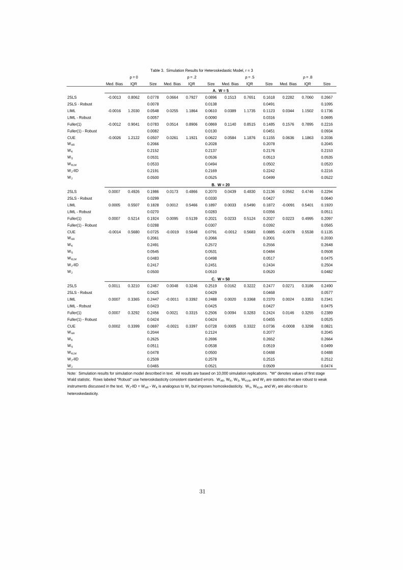
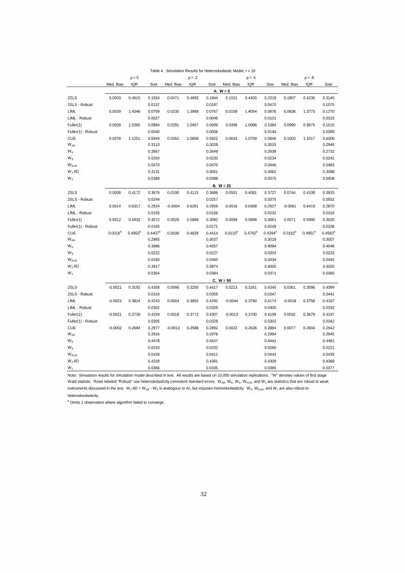
First, we consider the performance of the testing procedures in terms of size of tests. In

particular, we consider rejection rates of the null hypothesis for 5% level tests based on the

weak instrument robust test statistics discussed in this paper and based on standard χ2 tests

from conventional asymptotic theory. The results are quite favorable for our simple weak

instrument robust tests that are also robust to heteroskedasticity which do not appear to

suffer from large size distortions, though it is the case that WS and WJ are both conservative

when r = 10 in the sense that their actual rejection probabilities tend to be smaller than the

level of the test. On the other hand, the weak instrument robust tests that are not robust to

heteroskedasticity are severely size distorted with rejection rates between .1171 and .4507.

13To estimate the CUE, we numerically optimized the CUE objective function, which for a particular

value of β0 is given by the S-statistic of Stock and Wright (2000), using the default Newton-Raphson routine

in MATLAB.14Define A = X ′X − k(X ′X − X ′Z(Z ′Z)−1Z ′X) and B = Vxx − k(Vxx − X ′Z(Z ′Z)−1Vzx) − k(Vxx −

V ′zx(Z ′Z)−1Z ′X)+k2(Vxx− V ′

zx(Z ′Z)−1Z ′X−X ′Z(Z ′Z)−1Vzx+X ′Z(Z ′Z)−1Vzz(Z′Z)−1Z ′X) where Vgh =∑n

i=1ǫ2i gih

′i in the Robust case and Vgh = bǫ′bǫ

n−r−1G′H in the homoskedastic case. For LIML, we set k = φ

where φ is the minimum eigenvalue of (Y X)′(Y X)[(Y X)′(Y X)− (Y X)′PZ(Y X)]−1 and ǫ = Y − XβLIML;

and for Fuller, we set k = φ−1/(n−r−1) and ǫ = Y −XβFuller . Then for LIML and Fuller, we estimate the

covariance matrix as A−1BA−1. It is straightforward to verify consistency of these estimators under strong

instruments and the usual asymptotics.20

For the tests that are not robust to weak instruments, the results are somewhat different.

When the value of W is 50, tests based on 2SLS, LIML, and Fuller perform quite well and do

not appear to suffer from large size distortions.15 For smaller values of W , the size of LIML,

Fuller, and 2SLS based tests all depend heavily on the value of ρ and r. In particular, the

tests tend to over-reject when ρ and r are large and under-reject when ρ and r are small.

This dependence is especially pronounced for 2SLS, though it is present for all three of the

estimators.

Finally, it is worth noting that the CUE-based tests are badly size distorted in almost all

cases. Since the bias of the CUE is usually quite small and similar to LIML, it seems that

the source of this size distortion is poor performance of the CUE standard error estimates.

Both WS and WKLM are minimized at the CUE estimate, suggesting that they provide a

useful method of obtaining reasonable estimates of the CUE confidence intervals even in the

case of strong instruments.

Figure 1 plots power curves in the case of strong instruments (W = 200) when ρ = .5.

For readability, only the power curves of WS, WKLM , WJ and LIML with robust standard

errors are plotted. When r = 1, the power curves of all the estimators are indistinguishable;

that is, there is no power loss to using any of the weak instrument robust procedures in this

case. For r > 1, the power curve of the LM-based statistic (WKLM) always lies within the

AR-based statistic (WS), illustrating the power loss associated with the AR-based statistics

in overidentified models. It is also interesting to note that since LIML is not the efficient

estimator but both WS and WKLM are based on the CUE the LIML power curve may actually

lie outside the WS (and WKLM) power curve when r > 1.16

Power curves for the W = 5 case are plotted in Figure 3. As in Figure 1, we plot only

the power curves of WS, WKLM , WJ and LIML with robust standard errors. The curves are

plotted for ρ = .5 which from Table 1 is the value of ρ for which the size of LIML is closest to

the nominal level. In this case, there is less agreement between the weak instrument robust

statistics than in the W = 200 case. The LM-based tests (WKLM and WJ) tend to have

15Though not reported, 2SLS based tests in the homoskedastic case do suffer from modest size distortions

when the W is 50.16We did not report the CUE in this case due to the previously mentioned poor performance of the CUE

standard error estimates.21

better power than WS against alternatives close to the true parameter value. However, WS

appears to have more power against more remote alternatives. The power curve for LIML is

centered away from the true parameter value, and has almost no power against alternatives

about its center. The performance of LIML in the weak instrument case depends strongly on

ρ. In particular, as ρ increases, the bias of LIML tends to increase and the spread decreases,

which translates into power curves whose centers shift away from the true parameter value

and which become more concentrated about the center as ρ increases. This behavior leads to

increases in the size of the tests as ρ increases; though it does lead to tests with approximately

correct size for moderate values of ρ.

When coupled with the size results, the power results strongly favor the use of weak

instrument robust procedures. The weak instrument robust procedures guard against the

potential size distortions which may arise due to weak instruments and also have good power

properties when the instruments are strong. In cases where r = 1, weak instrument robust

tests and confidence intervals may be constructed readily in any standard statistical package

through a series of OLS regressions of Y −Xb on Z for various values of b. In the overidentified

case, this procedure may also be followed, and the simulation results suggest that the power

loss relative to more complicated methods may be small in many settings. In addition, a

more powerful procedure may be obtained by transforming the instruments as discussed in

Section 3.

5. Empirical Example

To illustrate the use of weak instrument robust statistics and the differences which may

arise between the conventional asymptotic inference and the weak instrument robust infer-

ence, we present the results from a simple empirical example.17 The data are drawn from

the innovative paper of Acemoglu, Johnson, and Robinson (2001) which examines the effect

of institutions on economic performance using mortality rates among European colonists as

an instrument for current institutions. This paper provides a useful case to consider in that

there is some variation in the strength of the instruments across specifications as discussed

17Perhaps the most-often cited case of “weak instruments” is the returns to schooling paper of Angrist

and Krueger (1991). For a discussion of this paper in the weak instruments context and a reinterpretation

as a case of “too many” instruments, see Hansen, Hausman, and Newey (2005).22

below. In addition, the model is just-identified and so is typical in the sense that most

empirical analyses are based on just-identified empirical models.

We focus on the main set of results from Acemoglu, Johnson, and Robinson (2001) which

are found in their Table 4. These results correspond to a simple linear IV model of the form

given by

Y = Xβ + Wγ + ǫ

X = ZΠ + WΓ + V

which can be put into the form given by equations (1) and (2) above by partialing out W . In

this example, Y is the log of PPP adjusted GDP per capita in 1995, X is average protection

against expropriation risk from 1985 to 1995 which provides a measure of institutions and

well-enforced property rights, and W is a set of additional covariates which varies across

specifications and may include a normalized measure of distance from the equator (latitude)

as well as dummy variables for a country’s continent. Detailed descriptive statistics and data

descriptions are found in Acemoglu, Johnson, and Robinson (2001), and for brevity we do

not discuss them here.18

Table 5 reports the 2SLS estimate of β (Panel A) as well as the IVQR estimate of the

effect of institutions at the median (Panel B). Heteroskedasticity robust confidence intervals

constructed from both the standard asymptotic distribution and the weak-instrument robust

statistics are provided for both estimates. In this example, the model is just-identified, so

the weak-instrument robust intervals for 2SLS can be computed by running a series of OLS

regressions of Y − Xβ0 on Z and performing heteroskedasticity robust inference on the

hypothesis that the coefficient on Z equals 0, and the weak-instrument robust intervals for

IVQR can be obtained by running a series of conventional quantile regressions of Y −Xβ0 on

Z and performing heteroskedasticity robust inference on the hypothesis that the coefficient

on Z equals 0. For the purposes of this analysis, we construct the intervals by considering

β0 equally spaced at 0.001 unit intervals in the range [-1,4]. The first-stage Wald statistic

for the test that Π = 0 is also reported at the top of the table. The model and sample

18Specifically, we use data on GDP, institutions, and colonial mortality from Acemoglu, Johnson, and

Robinson (2001) Appendix Table A2 and data on latitude from La Porta, Lopez-de Silanes, Shleifer, and

Vishny (1999) Appendix B. Detailed data descriptions are given in Acemoglu, Johnson, and Robinson (2001)

Appendix Table A1.23

used varies across the columns of Table 5. All even numbered columns control for latitude

which has been argued to have a direct effect on economic performance, e.g. in Gallup,

Mellinger, and Sachs (1999), and is plausibly correlated to settler mortality which implies

that its exclusion may render the instrument invalid. Columns (3)-(8) vary from Columns

(1) and (2) by considering alternate samples or including continent specific dummy variables

to assess the sensitivity of the basic results and control for other potential geographic factors.

Considering first the Wald statistic (W ), we see that there is substantial variation in the

strength of the instruments across specifications. W ranges from 3.65 to 36.24. For low

values of W , we would expect that the usual asymptotic confidence intervals and the weak-

instrument robust confidence intervals to be different, while for values of W in the 30’s, we

would expect that the usual intervals and the weak-instrument robust intervals to be quite

close. For IVQR, the first stage F-statistic is not the appropriate measure of the strength of

the relationship which depends on a density weighted correlation between the endogenous

variable and instrument, except in the homoskedastic case. However, we would expect the

W to be informative about this value and anticipate a similar pattern of results for IVQR.

Considering first the 2SLS results (Panel A), we observe the expected pattern in the actual

results. In columns (5) and (6) of Table 7, where the relationship between the instrument and

endogenous variable is the strongest (W above 30), the usual 95% confidence intervals and

the weak-instrument intervals are quite similar. The weak-instrument intervals are somewhat

wider, but the difference is not pronounced. As W decreases, the differences become much

larger. In particular, in the four cases with W < 10, the upper limit of the confidence interval

is equal to the upper limit of the set we consider for β0 and is much larger than the upper

limit of the usual confidence intervals. In the two remaining cases with W ≈ 12, the upper

bounds of the intervals are much larger than those of the usual intervals, but remain within

the interval considered for β0.

It is extremely interesting to note that in all cases the weak-instrument intervals provide

a sharp lower bound on the value of β. Even when W is low and the 95% weak-instrument

robust intervals appear to be unbounded on one side, the weak-instrument intervals have

a positive lower bound that is removed from zero. In other words, in this example even

when the data are not informative about an upper bound on β, they seem to have power to

rule out small positive and negative values for β. This finding is quite useful as it provides

24

strong evidence that institutions do matter for GDP and that the lower bound on the effect

is still substantial. In addition, we should be able to rule out large positive values for β as

they would imply implausibly large effects of institutions on per capita GDP. For example,

the difference in expropriation risk between Nigeria and Chile is 2.24. If β were 3, then

this difference would imply a 6.72 log-point (roughly 800-fold) difference in per capita GDP.

This number is ridiculously large. Thus, we see that even in cases where the instruments

are weak, the data may still inform us about the actual parameter values and allow us to

make economically useful inferences. However, this example also illustrates that there may

be large differences in the confidence intervals which could dramatically alter the inference.

Turning to the IVQR estimates of the effect at the median (Panel B), we see that the 2SLS

and IVQR point estimates are quite similar in all cases. However, the IVQR estimates are

considerably less precise than the corresponding 2SLS estimates, and it is difficult to draw

any firm conclusion from them. In terms of the confidence intervals, we see that, as with

the 2SLS intervals, the weak-instrument robust intervals are always considerably wider than

the asymptotic intervals. In addition, the differences between the intervals follow the same

patterns as in the 2SLS case, with relatively small differences in the cases where W is large

and substantially bigger differences as W decreases.

As a final illustration of the weak-instrument robust confidence intervals. We plot 1 minus

the p-value for testing β = β0 in two representative cases from Table 5 in Figure 5. The first

panel of Figure 5 corresponds to column (1) of Table 5 Panel A in which the weak-instrument

confidence interval is contained in the interval for β0 that we consider. The second panel

corresponds to column (7) of Table 5 Panel A in which the upper limit of the weak instrument

interval is equal to the upper limit of the interval we consider for β0. In both panels, the

horizontal line is drawn at 1 - p-value = .95, so the 95% confidence interval is given by the

values of β0 for which the 1 - p-value lies below this line. In the first case, the 1 - p-value

rises above .95 and stays well above it as β0 approaches the endpoints of the plotted region.

In the second case, the 1 - p-value is considerably below .95 as β0 approaches 4, the upper

limit of the region. That is, the confidence interval for β in this case may be substantially

wider than the interval given in Table 5. However, since large values for β imply implausibly

large effects, we ignore values for β0 greater than 4.

25

6. Conclusion

In this paper, we have considered practical implementation of weak-instrument robust

testing procedures in the linear IV model with possible heteroskedasticity or autocorrelation.

We show that weak-instrument robust procedures that are also robust to heteroskedasticity

or autocorrelation for testing the hypothesis that β = β0 may easily be constructed through

linear regression of a transformed dependent variable, Y − Xβ0, on the set of instruments,

Z, where X is the set of endogenous variables. This approach provides a practical and easy

to implement procedure for testing in the presence of weak instruments and may easily be

adapted to construct confidence intervals for β. We illustrate how the basic approach may be

adapted to improve power in cases where the model is overidentified, and we also discuss how

the procedure may be adapted to obtain valid confidence intervals under weak-identification

for parameters of an instrumental variables quantile regression model.

We have illustrated the properties of the test procedures through a simulation study and a

brief empirical example. The results from the simulation study confirm the theoretical results

and show that the weak-instrument robust test procedures have approximately correct size

regardless of the strength of the instruments. In addition, the simulations illustrate that

when the instruments are strong, there is no loss of power from using weak instrument

robust statistics. The simulation results also demonstrate the loss of power that can occur

when the model is overidentified and one does not transform the instruments as discussed in

the paper, though in many reasonable cases this power loss appears to be small. The results

from the empirical example illustrate the potential large differences that may exist between

conventional inference procedures and weak-instrument robust inference procedures. The

empirical results also show that interesting conclusions can be drawn when weak instrument

robust inference is performed even in cases where the instruments are weak and confidence

intervals are possibly unbounded.

References

Acemoglu, D., S. Johnson, and J. A. Robinson (2001): “The Colonial Origins of Comparative Devel-opment: An Empirical Investigation,” American Economic Review, 91(5), 1369–1401.

Anderson, T. W., and H. Rubin (1949): “Estimation of the Parameters of Single Equation in a CompleteSystem of Stochastic Equations,” Annals of Mathematical Statistics, 20, 46–63.

Andrews, D. W. K. (1991): “Heteroskedasticity and Autocorrelation Consistent Covariance Matrix Esti-mation,” Econometrica, 59(3), 817–858.

26

Andrews, D. W. K., M. J. Moreira, and J. H. Stock (2004a): “Heteroskedasticity and Autocorrela-tion Robust Inference with Weak Instruments,” working paper, Cowles Foundation.

(2004b): “Optimal Invariant Similar Tests for Instrumental Variables Regression with Weak In-struments,” Cowles Foundation Discussion Paper No. 1476.

Andrews, D. W. K., and J. H. Stock (2005): “Inference with Weak Instruments,” Cowles FoundationDiscussion Paper No. 1530.

Angrist, J. D., and A. Krueger (1991): “Does Compulsory Schooling Attendance Affect Schooling andEarnings,” Quarterly Journal of Economics, 106, 979–1014.

Angrist, J. D., and A. B. Krueger (2001): “Instrumental Variables and the Search for Identification:From Supply and Demand to Natural Experiments,” Journal of Economic Perspectives, 15, 69–85.

Arellano, M. (1987): “Computing Robust Standard Errors for Within-Groups Estimators,” Oxford Bul-letin of Economics and Statistics, 49(4), 431–434.

Bekker, P. A. (1994): “Alternative Approximations to the Distributions of Instrumental Variables Esti-mators,” Econometrica, 63, 657–681.

Chernozhukov, V., and C. Hansen (2004): “Instrumental Quantile Regression Inference for Structuraland Treatment Effect Models,” Journal of Econometrics (forthcoming).

Dufour, J.-M., and J. Jasiac (2001): “Finite Sample Limited Information Inference Methods for Struc-tural Equations and Models with Generated Regressors,” International Economic Review, 42, 815–843.

Dufour, J.-M., and M. Taamouti (2005): “Projection-Based Statistical Inference in Linear StructuralModels with Possibly Weak Instruments,” Econometrica, 73, 1351–1367.

Fitzenberger, B. (1998): “The Moving Blocks Bootstrap and Robust Inference in Linear Least Squaresand Quantile Regressions,” Journal of Econometrics, 82(2), 235–287.

Fuller, W. A. (1977): “Some Properties of a Modification of the Limited Information Estimator,” Econo-metrica, 45, 939–954.

Gallup, J. L., A. Mellinger, and J. D. Sachs (1999): “Geography and Economic Development,”International Regional Science Review, 22, 179–232.

Gutenbrunner, C., and J. Jureckova (1992): “Regression rank scores and regression quantiles,” Ann.Statist., 20(1), 305–330.

Hahn, J., J. A. Hausman, and G. M. Kuersteiner (2004): “Estimation with Weak Instruments:Accuracy of Higher-order Bias and MSE Approximations,” Econometrics Journal, 7(1), 272–306.

Hansen, C., J. Hausman, and W. K. Newey (2005): “Estimation with Many Instrumental Variables,”mimeo.

Hansen, L. P., J. Heaton, and A. Yaron (1996): “Finite Sample Properties of Some Alternative GMMEstimators,” Journal of Business and Economic Statistics, 14(3), 262–280.

Jansson, M. (2004): “The Error in Rejection Probability of Simple Autocorrelation Robust Tests,” Econo-metrica, 72(3), 937–946.

Kiefer, N. M., and T. J. Vogelsang (2002): “Heteroskedasticity-Autocorrelation Robust Testing UsingBandwidth Equal to Sample Size,” Econometric Theory, 18, 1350–1366.

Kleibergen, F. (2002): “Pivotal Statistics for Testing Structural Parameters in Instrumental VariablesRegression,” Econometrica, 70, 1781–1803.

(2004): “Generalizing Weak Instrument Robust IV Statistics Towards Multiple Parameters, Unre-stricted Covariance Matrices, and Identification Statistics,” Mimeo.

(2005): “Testing Parameters in GMM Without Assuming That They Are Identified,” Econometrica,73, 1103–1124.

Koenker, R. (1994): “Confidence intervals for regression quantiles,” in Asymptotic statistics (Prague,1993), pp. 349–359. Physica, Heidelberg.

La Porta, R., F. Lopez-de Silanes, A. Shleifer, and R. Vishny (1999): “The Quality of Govern-ment,” Journal of Law, Economics, and Organization, 15(1), 222–279.

Moreira, M. J. (2003): “A Conditional Likelihood Ratio Test for Structural Models,” Econometrica, 71,1027–1048.

Rothenberg, T. J. (1984): “Approximating the Distributions of Econometric Estimators and Test Sta-tistics,” in Handbook of Econometrics. Volume 2, ed. by Z. Griliches, and M. D. Intriligator. Elsevier:North-Holland.

Stock, J. H., and J. H. Wright (2000): “GMM with Weak Identification,” Econometrica, 68, 1055–1096.

27

Stock, J. H., J. H. Wright, and M. Yogo (2002): “A Survey of Weak Instruments and Weak Identifi-cation in Generalized Method of Moments,” Journal of Business and Economic Statistics, 20(4), 518–529.

White, H. (1980): “A Heteroskedasticity-Consistent Covariance Matrix Estimator and a Direct Test forHeteroskedasticity,” Econometrica, 48(4), 817–838.

(2001): Asymptotic Theory for Econometricians. San Diego: Academic Press, revised edn.Zivot, E., R. Startz, and C. R. Nelson (1998): “Valid Confidence Intervals and Inference in thePresence of Weak Instruments,” International Economic Review, 39, 1119–1144.

28

N* Mean 10th 25th 50th 75th 90th

Sample Size 220 39491 60 106 1577 55495 152742

Number of Instruments 261 2.89 1 1 1 3 10

First Stage Wald Statistic 221 140.31 7.22 11.56 22.02 67.65 637.97

Correlation 126 0.375 0.021 0.045 0.333 0.652 0.812

Sample Size 38 7272 64 200 700 4965 17649

Number of Instruments 56 3.55 1 1 2 4 9

First Stage Wald Statistic 28 142.06 7.53 12.51 22.58 117.32 722.27

Correlation 22 0.293 0.026 0.041 0.267 0.529 0.559

well as the mean and various percentiles of the distribution.correlation between the first stage and structural error terms. For each variable, we report the number of nonmissing observations, N*, as

within paper medians as unique observations. In each panel, we report summary statistics for the sample size used in estimating the firststage relationship, the number of instruments, the first stage Wald statistic for testing for relevance of the excluded instruments, and the

Table 1. Summary Statistics for Survey of IV Papers from AER, JPE, and QJE 1999-2004

Note: This table reports summary statistics for a survey of linear IV papers published in various issues of the American Economic Review,Journal of Political Economy, and Quarterly Journal of Economics in 1999-2004. The exact issues are given in the main text. The toppanel reports results where each unique first stage is treated as an observation, and the bottom panel reports results which treat the

A. One Observation per First Stage

B. One Observation per Paper

29

Med. Bias IQR Size Med. Bias IQR Size Med. Bias IQR Size Med. Bias IQR Size

2SLS -0.0020 0.7896 0.0177 -0.0004 0.7969 0.0284 0.0090 0.8092 0.0711 0.0217 0.7981 0.1338

2SLS - Robust 0.0055 0.0084 0.0345 0.0768

Fuller(1) -0.0007 0.5885 0.0336 0.0458 0.5941 0.0540 0.1125 0.5669 0.1276 0.1758 0.5062 0.2136

Fuller(1) - Robust 0.0105 0.0220 0.0717 0.1302

WAR 0.1232 0.1262 0.1209 0.1224

WS 0.0541 0.0497 0.0525 0.0532

2SLS -0.0046 0.5558 0.0445 -0.0048 0.5457 0.0501 -0.0041 0.5560 0.0869 -0.0084 0.5682 0.1269

2SLS - Robust 0.0136 0.0207 0.0417 0.0692

Fuller(1) -0.0042 0.4932 0.0559 0.0178 0.4830 0.0651 0.0455 0.4760 0.1061 0.0696 0.4551 0.1611

Fuller(1) - Robust 0.0181 0.0263 0.0535 0.0914

WAR 0.1208 0.1171 0.1234 0.1289

WS 0.0510 0.0543 0.0536 0.0555

2SLS -0.0017 0.3892 0.0814 -0.0004 0.3858 0.0818 0.0039 0.3869 0.0960 0.0032 0.3865 0.1142

2SLS - Robust 0.0329 0.0324 0.0398 0.0578

Fuller(1) -0.0015 0.3685 0.0861 0.0089 0.3653 0.0884 0.0282 0.3622 0.1079 0.0406 0.3488 0.1369

Fuller(1) - Robust 0.0351 0.0351 0.0482 0.0725

WAR 0.1239 0.1237 0.1254 0.1243

WS 0.0546 0.0541 0.0522 0.0527

2SLS -0.0044 0.2411 0.1094 0.0014 0.2435 0.1048 -0.0003 0.2449 0.1117 -0.0045 0.2491 0.1052

2SLS - Robust 0.0452 0.0431 0.0469 0.0493

Fuller(1) -0.0042 0.2362 0.1102 0.0053 0.2386 0.1070 0.0094 0.2385 0.1151 0.0110 0.2394 0.1145

Fuller(1) - Robust 0.0459 0.0439 0.0505 0.0549

WAR 0.1250 0.1218 0.1243 0.1208

WS 0.0565 0.0515 0.0514 0.0503

2SLS -0.0017 0.1218 0.1215 -0.0004 0.1203 0.1147 -0.0003 0.1191 0.1150 -0.0003 0.1186 0.1131

2SLS - Robust 0.0544 0.0496 0.0515 0.0507

Fuller(1) -0.0017 0.1210 0.1212 0.0006 0.1197 0.1149 0.0020 0.1181 0.1163 0.0036 0.1176 0.1170

Fuller(1) - Robust 0.0544 0.0499 0.0514 0.0517

WAR 0.1241 0.1185 0.1173 0.1177

WS 0.0556 0.0501 0.0515 0.0523

and WS is also heteroskedasticity robust.

ρ = 0 ρ = .2 ρ = .5 ρ = .8

Wald statistic. Rows labeled "Robust" use heteroskdasticity consistent standard errors. WAR and WS are statistics that are robust to weak instruments,

D. W = 50

E. W = 200

Note: Simulation results for simulation model described in text. All results are based on 10,000 simulation replications. "W" denotes values of first stage

Table 2. Simulation Results for Heteroskedastic Model, r = 1

A. W = 5

B. W = 10

C. W = 20

30

Med. Bias IQR Size Med. Bias IQR Size Med. Bias IQR Size Med. Bias IQR Size

2SLS -0.0013 0.8062 0.0778 0.0664 0.7927 0.0896 0.1513 0.7651 0.1618 0.2282 0.7060 0.2667

2SLS - Robust 0.0078 0.0138 0.0491 0.1095

LIML -0.0016 1.2030 0.0548 0.0255 1.1864 0.0610 0.0389 1.1735 0.1123 0.0344 1.1502 0.1736

LIML - Robust 0.0057 0.0090 0.0316 0.0695

Fuller(1) -0.0012 0.9041 0.0783 0.0514 0.8906 0.0869 0.1140 0.8515 0.1485 0.1576 0.7895 0.2216

Fuller(1) - Robust 0.0082 0.0130 0.0451 0.0934

CUE -0.0026 1.2122 0.0507 0.0261 1.1921 0.0622 0.0584 1.1876 0.1155 0.0636 1.1863 0.2036

WAR 0.2066 0.2028 0.2078 0.2045

WK 0.2152 0.2137 0.2176 0.2153

WS 0.0531 0.0536 0.0513 0.0535

WKLM 0.0533 0.0494 0.0502 0.0520

WJ-IID 0.2191 0.2169 0.2242 0.2216

WJ 0.0500 0.0525 0.0499 0.0522

2SLS 0.0007 0.4926 0.1986 0.0173 0.4866 0.2070 0.0439 0.4830 0.2136 0.0562 0.4746 0.2294

2SLS - Robust 0.0299 0.0330 0.0427 0.0640

LIML 0.0005 0.5507 0.1828 0.0012 0.5466 0.1897 0.0033 0.5490 0.1872 -0.0091 0.5401 0.1920

LIML - Robust 0.0270 0.0283 0.0356 0.0511

Fuller(1) 0.0007 0.5214 0.1924 0.0095 0.5139 0.2021 0.0233 0.5124 0.2027 0.0223 0.4995 0.2097

Fuller(1) - Robust 0.0288 0.0307 0.0392 0.0565

CUE -0.0014 0.5680 0.0725 -0.0019 0.5648 0.0791 -0.0012 0.5683 0.0885 -0.0078 0.5538 0.1135

WAR 0.2061 0.2066 0.2001 0.2030

WK 0.2491 0.2572 0.2556 0.2648

WS 0.0545 0.0531 0.0484 0.0508

WKLM 0.0483 0.0498 0.0517 0.0475

WJ-IID 0.2417 0.2451 0.2434 0.2504

WJ 0.0500 0.0510 0.0520 0.0482

2SLS 0.0011 0.3210 0.2467 0.0048 0.3246 0.2519 0.0162 0.3222 0.2477 0.0271 0.3186 0.2490

2SLS - Robust 0.0425 0.0429 0.0468 0.0577

LIML 0.0007 0.3365 0.2447 -0.0011 0.3392 0.2488 0.0020 0.3368 0.2370 0.0024 0.3353 0.2341

LIML - Robust 0.0423 0.0425 0.0427 0.0475

Fuller(1) 0.0007 0.3292 0.2456 0.0021 0.3315 0.2506 0.0094 0.3283 0.2424 0.0146 0.3255 0.2389

Fuller(1) - Robust 0.0424 0.0424 0.0455 0.0525

CUE 0.0002 0.3399 0.0697 -0.0021 0.3397 0.0728 0.0005 0.3322 0.0736 -0.0008 0.3298 0.0821

WAR 0.2044 0.2124 0.2077 0.2045

WK 0.2625 0.2696 0.2652 0.2664

WS 0.0511 0.0538 0.0519 0.0499

WKLM 0.0478 0.0500 0.0488 0.0488

WJ-IID 0.2509 0.2578 0.2515 0.2512

WJ 0.0465 0.0521 0.0509 0.0474

ρ = .8

Wald statistic. Rows labeled "Robust" use heteroskdasticity consistent standard errors. WAR, WK, WS, WKLM, and WJ are statistics that are robust to weak

Note: Simulation results for simulation model described in text. All results are based on 10,000 simulation replications. "W" denotes values of first stage

B. W = 20

C. W = 50

Table 3. Simulation Results for Heteroskedastic Model, r = 3

A. W = 5

heteroskedasticity.

instruments discussed in the text. WJ-IID = WAR - WK is analogous to WJ but imposes homoskedasticity. WS, WKLM, and WJ are also robust to

ρ = 0 ρ = .2 ρ = .5

31

Med. Bias IQR Size Med. Bias IQR Size Med. Bias IQR Size Med. Bias IQR Size

2SLS 0.0003 0.4615 0.1934 0.0471 0.4693 0.1944 0.1021 0.4400 0.2318 0.1807 0.4236 0.3140

2SLS - Robust 0.0137 0.0197 0.0470 0.1075

LIML 0.0029 1.4346 0.0709 0.0230 1.3989 0.0767 0.0159 1.4054 0.0876 0.0636 1.3775 0.1270

LIML - Robust 0.0027 0.0045 0.0101 0.0315

Fuller(1) 0.0028 1.0365 0.0894 0.0291 1.0407 0.0939 0.0396 1.0086 0.1084 0.0990 0.9875 0.1515

Fuller(1) - Robust 0.0040 0.0056 0.0144 0.0395

CUE 0.0078 1.1251 0.5944 0.0262 1.0808 0.5922 0.0633 1.0709 0.5846 0.1003 1.1017 0.6306

WAR 0.3113 0.3028 0.3015 0.2946

WK 0.2667 0.2649 0.2638 0.2732

WS 0.0250 0.0233 0.0234 0.0241

WKLM 0.0470 0.0470 0.0446 0.0483

WJ-IID 0.3131 0.3051 0.3062 0.3088

WJ 0.0389 0.0398 0.0375 0.0408

2SLS 0.0008 0.4172 0.3676 0.0190 0.4115 0.3686 0.0501 0.4081 0.3727 0.0764 0.4108 0.3933

2SLS - Robust 0.0244 0.0257 0.0375 0.0552

LIML 0.0014 0.6317 0.2924 -0.0004 0.6261 0.2959 0.0016 0.6308 0.2927 -0.0061 0.6419 0.2870

LIML - Robust 0.0155 0.0156 0.0232 0.0316

Fuller(1) 0.0012 0.5932 0.3072 0.0026 0.5868 0.3092 0.0099 0.5898 0.3061 0.0071 0.5990 0.3025

Fuller(1) - Robust 0.0165 0.0171 0.0249 0.0338

CUE 0.0016a 0.4953a 0.4407a 0.0039 0.4828 0.4414 0.0133a 0.4792a 0.4394a 0.0162a 0.4951a 0.4563a

WAR 0.2965 0.3037 0.3019 0.3007

WK 0.3986 0.4057 0.4094 0.4048

WS 0.0222 0.0227 0.0203 0.0233

WKLM 0.0430 0.0460 0.0434 0.0445

WJ-IID 0.3917 0.3974 0.4000 0.4020

WJ 0.0364 0.0384 0.0371 0.0385

2SLS -0.0021 0.3192 0.4358 0.0096 0.3250 0.4417 0.0213 0.3161 0.4340 0.0361 0.3096 0.4399

2SLS - Robust 0.0316 0.0359 0.0347 0.0441

LIML -0.0023 0.3824 0.4243 0.0004 0.3855 0.4292 -0.0044 0.3780 0.4174 -0.0018 0.3758 0.4167

LIML - Robust 0.0302 0.0325 0.0300 0.0332

Fuller(1) -0.0021 0.3739 0.4259 0.0018 0.3772 0.4307 -0.0013 0.3700 0.4199 0.0032 0.3679 0.4197

Fuller(1) - Robust 0.0305 0.0329 0.0302 0.0342

CUE -0.0002 0.2684 0.2977 -0.0013 0.2588 0.2892 0.0022 0.2626 0.2884 0.0077 0.2604 0.2942

WAR 0.2916 0.2976 0.2994 0.2945

WK 0.4478 0.4507 0.4441 0.4481

WS 0.0233 0.0232 0.0260 0.0221

WKLM 0.0428 0.0412 0.0443 0.0435

WJ-IID 0.4328 0.4381 0.4309 0.4368

WJ 0.0366 0.0335 0.0385 0.0377

Table 4. Simulation Results for Heteroskedastic Model, r = 10

A. W = 5

heteroskedasticity.

instruments discussed in the text. WJ-IID = WAR - WK is analogous to WJ but imposes homoskedasticity. WS, WKLM, and WJ are also robust to

ρ = 0 ρ = .2 ρ = .5 ρ = .8

Wald statistic. Rows labeled "Robust" use heteroskdasticity consistent standard errors. WAR, WK, WS, WKLM, and WJ are statistics that are robust to weak

Note: Simulation results for simulation model described in text. All results are based on 10,000 simulation replications. "W" denotes values of first stage

a Omits 1 observation where algorithm failed to converge.

B. W = 20

C. W = 50

32

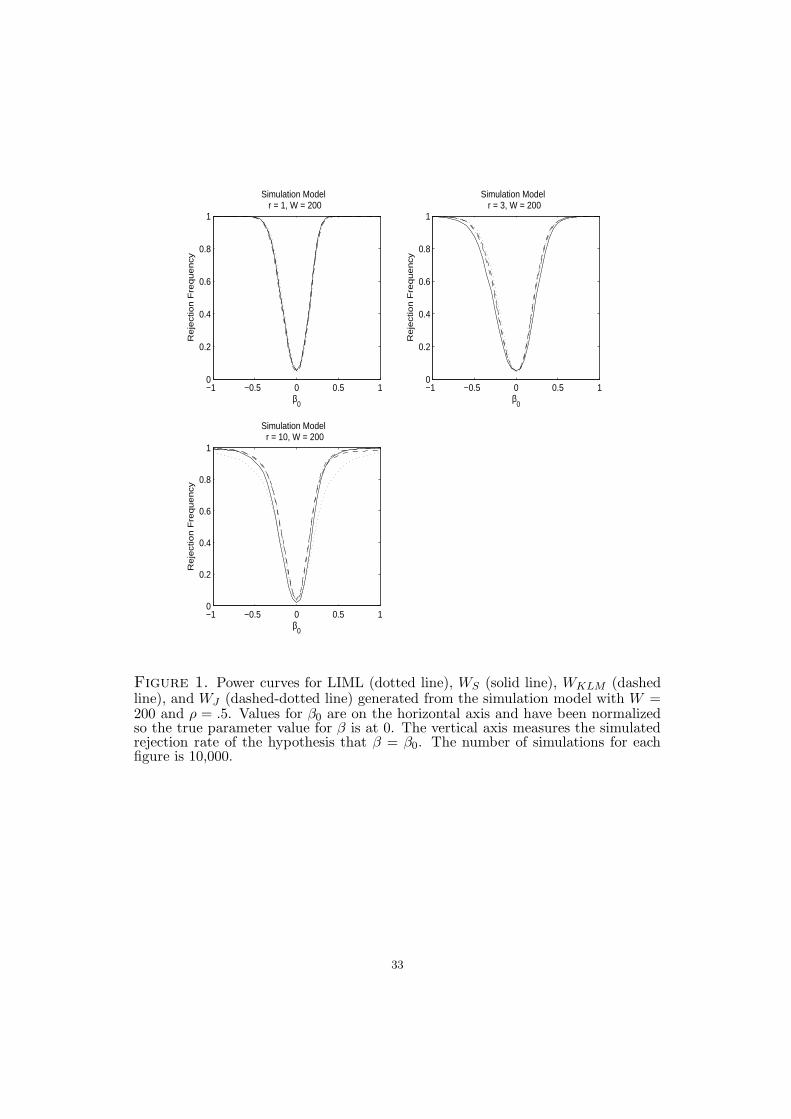
−1 −0.5 0 0.5 10

0.2

0.4

0.6

0.8

1

β0

Re

ject

ion

Fre

qu

en

cySimulation Model

r = 1, W = 200

−1 −0.5 0 0.5 10

0.2

0.4

0.6

0.8

1

β0

Re

ject

ion

Fre

qu

en

cy

Simulation Modelr = 3, W = 200

−1 −0.5 0 0.5 10

0.2

0.4

0.6

0.8

1

β0

Re

ject

ion

Fre

qu

en

cy

Simulation Modelr = 10, W = 200

Figure 1. Power curves for LIML (dotted line), WS (solid line), WKLM (dashedline), and WJ (dashed-dotted line) generated from the simulation model with W =200 and ρ = .5. Values for β0 are on the horizontal axis and have been normalizedso the true parameter value for β is at 0. The vertical axis measures the simulatedrejection rate of the hypothesis that β = β0. The number of simulations for eachfigure is 10,000.

33

−1 −0.5 0 0.5 10

0.1

0.2

0.3

0.4

0.5

β0

Re

jectio

n F

req

ue

ncy

Simulation Modelr = 1, W = 5

−1 −0.5 0 0.5 10

0.05

0.1

0.15

0.2

0.25

0.3

0.35

0.4

β0

Re

jectio

n F

req

ue

ncy

Simulation Modelr = 3, W = 5

−1 −0.5 0 0.5 10

0.05

0.1

0.15

0.2

0.25

0.3

0.35

β0

Re

jectio

n F

req

ue

ncy

Simulation Modelr = 10, W = 5

Figure 2. Power curves for LIML (dotted line), WS (solid line), WKLM (dashedline), and WJ (dashed-dotted line) generated from the simulation model with W =5 and ρ = .5. Values for β0 are on the horizontal axis and have been normalizedso the true parameter value for β is at 0. The vertical axis measures the simulatedrejection rate of the hypothesis that β = β0. The number of simulations for eachfigure is 10,000.

34

Base Sample Base Sample

Base Sample without Neo-

Europes

Base Sample without Neo-

EuropesBase Sample without Africa

Base Sample without Africa Base Sample Base Sample

(1) (2) (3) (4) (5) (6) (7) (8)

N 64 64 60 60 37 37 64 64

W 16.322 12.110 6.917 6.150 36.240 27.563 5.244 3.648

Latitude Y Y Y Y

Continent Dummies Y Y�2SLS 0.924 0.969 1.236 1.219 0.578 0.576 0.932 1.026

Asymptotic Interval (0.580,1.267) (0.544,1.395) (0.461,2.011) (0.424,2.013) (0.408,0.749) (0.384,0.768) (0.281,1.583) (0.114,1.938)

Weak-Instrument Interval (0.662,1.667) (0.653,2.066) (0.731,4] (0.709,4] (0.418,0.816) (0.378,0.832) (0.443,4] (0.357,4]�(.50) 1.272 1.348 1.320 1.320 0.535 0.544 0.934 0.991

Asymptotic Interval (-0.491,3.035) (-0.723,3.419) (-0.505,3.145) (-0.694,3.334) (0.326,0.744) (0.298,0.790) (-0.763,2.631) (-0.808,2.790)

Weak-Instrument Interval (0.155,4] (0.132,4] (0.152,4] [-1,4] (0.390,1.089) (0.076,1.170) [-1,4] [-1,4]

Columns (5) and (6) omit all African countries.

W is the the first-stage Wald statistic for testing instrument irrelevance, and N is the the sample size. Even numbered columns include latitude as anexplanatory variable, and columns (7) and (8) include continent dummy variables. Columns (3) and (4) omit Australia, Canada, New Zealand, and the USA.

Table 5. IV and Median IV Regressions of Log GDP per Capita on Institutions

Note: This table reports the 2SLS estimate of the effect of institutions on GDP (�

2SLS) and the IVQR estimate of the effect of institutions on GDP at themedian (

�(.50)). Asymptotic Interval reports the 95% confidence interval constructed using the usual asymptotic approximation, and Weak-Instrument

Interval reports the 95% confidence interval constructed using the weak-instrument robust statistic. Both intervals account for possible heteroskedasticity.

A. 2SLS Results

B. IVQR Results

35

−1 0 1 2 3 40

0.1

0.2

0.3

0.4

0.5

0.6

0.7

0.8

0.9

1

β0

1 −

p−

valu

e

(1)

−1 0 1 2 3 40

0.1

0.2

0.3

0.4

0.5

0.6

0.7

0.8

0.9

1

β0

1 −

p−

valu

e

(2)

Figure 3. 1 - p-value plots for typical cases from empirical example. Panel (1)corresponds to column (1) in Table 5 Panel A, and Panel (2) corresponds to column(7) in Table 5 Panel A. The vertical axis is 1 minus the p-value for a test of thehypothesis that β = β0 performed using the heteroskedasticity and weak-instrumentrobust statistic WS . The horizontal axis corresponds to β0. The 95% confidenceinterval is given by the region of the plot where 1 - p-value lies below .95. Ahorizontal line has been drawn in at 1 - p-value = .95 for clarity. β is a measure ofthe impact of institutions on economic performance as discussed in the text.

36