the regular histories formulation of quantum theory regular histories formulation of quantum theory...
TRANSCRIPT

The Regular Histories Formulation
of Quantum Theory
DPhil Thesis
Roman PriebeMerton College, Oxford
Trinity Term 2012

Abstract
A measurement-independent formulation of quantum mechanics called ‘regular histories’
(RH) is presented, able to reproduce the predictions of the standard formalism without
the need to for a quantum-classical divide or the presence of an observer. It applies to
closed systems and features no wave-function collapse.
Weights are assigned only to histories satisfying a criterion called ‘regularity’. As the set
of regular histories is not closed under the Boolean operations this requires a new con-
cept of weight, called ‘likelihood’. Remarkably, this single change is enough to overcome
many of the well-known obstacles to a sensible interpretation of quantum mechanics. For
example, Bell’s theorem, which makes essential use of probabilities, places no constraints
on the locality properties of a theory based on likelihoods. Indeed, RH is both counter-
factually definite and free from action-at-a-distance.
Moreover, in RH the meaningful histories are exactly those that can be witnessed at least
in principle. Since it is especially difficult to make sense of the concept of probability for
histories whose occurrence is intrinsically indeterminable, this makes likelihoods easier
to justify than probabilities.
Interaction with the environment causes the kinds of histories relevant at the macroscopic
scale of human experience to be witnessable and indeed to generate Boolean algebras of
witnessable histories, on which likelihoods reduce to ordinary probabilities. Further-
more, a formal notion of inference defined on regular histories satisfies, when restricted
to such Boolean algebras, the classical axioms of implication, explaining our perception
of a largely classical world.
Even in the context of general quantum histories the rules of reasoning in RH are remark-
ably intuitive. Classical logic must only be amended to reflect the fundamental premise
that one cannot meaningfully talk about the occurrence of unwitnessable histories.
Crucially, different histories with the same ‘physical content’ can be interpreted in the
same way and independently of the family in which they are expressed. RH thereby
rectifies a critical flaw of its inspiration, the consistent histories (CH) approach, which
requires either an as yet unknown set selection rule or a paradigm shift towards an un-
conventional picture of reality whose elements are histories-with-respect-to-a-framework.
It can be argued that RH compares favourably with other proposed interpretations of
quantum mechanics in that it resolves the measurement problem while retaining an
essentially classical worldview without parallel universes, a framework-dependent reality
or action-at-a-distance.

Acknowledgements
I am profoundly indebted to my supervisor Samson Abramsky for undertaking the Her-
culean task of battling through countless pages of barely comprehensible drafts. His
invaluable insights have turned this work into what it is today. I also thank Bob Coecke
and Andreas Doring for their generous feedback on my confirmation of status report
that sparked off great improvements and could not have come at a better time. I am
very grateful to Chris Isham and Adrian Kent for their constructive feedback. To Terry
Rudolph, who helped me out of a state of perfect confusion, and Jonathan Halliwell, who
kindly offered his time and opinion.
I cannot thank enough my friends and colleagues in the department, who have made my
time there worthwhile: Ray Lal, Andrei Akhvlediani, Pia Wojtinnek, Shane Mansfield,
Jamie Vicary, Janet Sadler and Prakash Panangaden to name but a few. Of course I
should also like to express my gratitude to the EPSRC for funding this research.
I am very fortunate in counting Konrad Leistikow, Sven Svoboda and Rafa l Szala among
my friends and in finding with Nathalie Thierjung the best distraction one could wish
for. Natalie McDaid brightened up my days throughout the final stretch of the writeup.
Pauline Rueckerl spurred me on to new heights of motivation, as did Alexandra Konzack
and Sara Gordon. No praise is too high for my friends at Merton, who I have spent
the happiest of times with: Stephanie Jones, Claire Higgins, Greg Lim, Joanne Lovesey,
Vanessa Johnen, Silvia Jonas, John Lee Allen, Lottie McIntyre, Kyle Martin and, of
course, Clement among many others. I would like to thank Merton College and its staff
for providing me with a truly paradisal environment and the community of MCR Presi-
dents for many joyous memories.
To my family I owe far more than I could hope to acknowledge here. I am supremely
grateful for their love, care and support.

Contents
1 Introduction 1
1.1 The standard formalism . . . . . . . . . . . . . . . . . . . . . . . . . . . . . . . . . . 1
1.2 The Copenhagen Interpretation . . . . . . . . . . . . . . . . . . . . . . . . . . . . . . 2
1.3 Bohmian mechanics . . . . . . . . . . . . . . . . . . . . . . . . . . . . . . . . . . . . 3
1.4 Many worlds . . . . . . . . . . . . . . . . . . . . . . . . . . . . . . . . . . . . . . . . 3
1.5 Consistent histories - a conceptual overview . . . . . . . . . . . . . . . . . . . . . . . 3
2 Definitions and technical background 7
2.1 Propositions . . . . . . . . . . . . . . . . . . . . . . . . . . . . . . . . . . . . . . . . . 7
2.2 Histories . . . . . . . . . . . . . . . . . . . . . . . . . . . . . . . . . . . . . . . . . . . 10
2.2.1 Fine- and coarse-graining . . . . . . . . . . . . . . . . . . . . . . . . . . . . . 12
2.2.2 The topos approach . . . . . . . . . . . . . . . . . . . . . . . . . . . . . . . . 15
2.3 The chain operator . . . . . . . . . . . . . . . . . . . . . . . . . . . . . . . . . . . . . 15
2.4 Weights and consistency . . . . . . . . . . . . . . . . . . . . . . . . . . . . . . . . . . 17
2.4.1 Mixed initial states . . . . . . . . . . . . . . . . . . . . . . . . . . . . . . . . . 17
2.4.2 Lack of additivity . . . . . . . . . . . . . . . . . . . . . . . . . . . . . . . . . 17
2.4.3 Consistency . . . . . . . . . . . . . . . . . . . . . . . . . . . . . . . . . . . . . 18
2.4.4 Decoherence . . . . . . . . . . . . . . . . . . . . . . . . . . . . . . . . . . . . . 18
2.4.5 Consistency of histories . . . . . . . . . . . . . . . . . . . . . . . . . . . . . . 19
2.4.6 Branch dependence . . . . . . . . . . . . . . . . . . . . . . . . . . . . . . . . . 21
2.4.7 Linear positivity . . . . . . . . . . . . . . . . . . . . . . . . . . . . . . . . . . 21
2.5 Conditional probabilities . . . . . . . . . . . . . . . . . . . . . . . . . . . . . . . . . . 22
2.6 Implication . . . . . . . . . . . . . . . . . . . . . . . . . . . . . . . . . . . . . . . . . 22
2.7 The single framework rule . . . . . . . . . . . . . . . . . . . . . . . . . . . . . . . . . 24
2.7.1 Compatible families . . . . . . . . . . . . . . . . . . . . . . . . . . . . . . . . 24
2.8 Measurements and observers . . . . . . . . . . . . . . . . . . . . . . . . . . . . . . . . 24
2.8.1 Reproducing the predictions of the standard formalism . . . . . . . . . . . . . 27
2.9 Approximate consistency . . . . . . . . . . . . . . . . . . . . . . . . . . . . . . . . . . 28
i

2.10 Sum-over-histories formulation . . . . . . . . . . . . . . . . . . . . . . . . . . . . . . 29
2.10.1 The EPE interpretation . . . . . . . . . . . . . . . . . . . . . . . . . . . . . . 29
2.11 IGUSes and the persistence of quasiclassicality . . . . . . . . . . . . . . . . . . . . . 30
2.12 Records . . . . . . . . . . . . . . . . . . . . . . . . . . . . . . . . . . . . . . . . . . . 31
2.12.1 Records imply decoherence . . . . . . . . . . . . . . . . . . . . . . . . . . . . 31
2.12.2 Decoherence implies records . . . . . . . . . . . . . . . . . . . . . . . . . . . . 32
2.13 The Diosi test . . . . . . . . . . . . . . . . . . . . . . . . . . . . . . . . . . . . . . . . 33
2.14 Examples . . . . . . . . . . . . . . . . . . . . . . . . . . . . . . . . . . . . . . . . . . 33
2.14.1 The Mach-Zehnder interferometer . . . . . . . . . . . . . . . . . . . . . . . . 33
2.14.2 Young’s double slit experiment . . . . . . . . . . . . . . . . . . . . . . . . . . 36
2.14.3 The Einstein-Podolsky-Rosen ‘paradox’ . . . . . . . . . . . . . . . . . . . . . 36
2.14.4 A consistent family that is not decoherent . . . . . . . . . . . . . . . . . . . . 37
3 Problems and criticism 38
3.1 Notions of truth in consistent histories . . . . . . . . . . . . . . . . . . . . . . . . . . 38
3.1.1 Notion of truth according to Omnes . . . . . . . . . . . . . . . . . . . . . . . 38
3.1.2 Notion of truth according to Griffiths . . . . . . . . . . . . . . . . . . . . . . 39
3.1.3 Notion of truth according to Gell-Mann and Hartle . . . . . . . . . . . . . . . 40
3.1.4 Notion of truth according to Dowker and Kent . . . . . . . . . . . . . . . . . 42
3.1.5 The EPE interpretation . . . . . . . . . . . . . . . . . . . . . . . . . . . . . . 42
3.2 Approximate consistency . . . . . . . . . . . . . . . . . . . . . . . . . . . . . . . . . . 43
3.3 Bell’s theorem and locality . . . . . . . . . . . . . . . . . . . . . . . . . . . . . . . . . 43
3.3.1 ‘Einstein locality’ in the CH approach . . . . . . . . . . . . . . . . . . . . . . 46
3.4 The Kochen-Specker Theorem . . . . . . . . . . . . . . . . . . . . . . . . . . . . . . . 47
3.5 Contrary inferences (CI) . . . . . . . . . . . . . . . . . . . . . . . . . . . . . . . . . . 51
3.5.1 Contrary inferences revisited . . . . . . . . . . . . . . . . . . . . . . . . . . . 56
3.6 Identification of histories . . . . . . . . . . . . . . . . . . . . . . . . . . . . . . . . . . 58
3.6.1 Embedding in families . . . . . . . . . . . . . . . . . . . . . . . . . . . . . . . 58
3.6.2 Inserting identities . . . . . . . . . . . . . . . . . . . . . . . . . . . . . . . . . 63
3.7 Changing the temporal support . . . . . . . . . . . . . . . . . . . . . . . . . . . . . . 64
3.8 Discussion . . . . . . . . . . . . . . . . . . . . . . . . . . . . . . . . . . . . . . . . . . 65
4 The regular histories interpretation 67
4.1 Mathematical formalism . . . . . . . . . . . . . . . . . . . . . . . . . . . . . . . . . . 68
4.1.1 Regular families . . . . . . . . . . . . . . . . . . . . . . . . . . . . . . . . . . 68
4.1.2 Likelihoods . . . . . . . . . . . . . . . . . . . . . . . . . . . . . . . . . . . . . 71
4.1.3 Notion of truth of regular histories . . . . . . . . . . . . . . . . . . . . . . . . 72
ii

4.1.4 Further properties of likelihoods . . . . . . . . . . . . . . . . . . . . . . . . . 72
4.2 Interpretation . . . . . . . . . . . . . . . . . . . . . . . . . . . . . . . . . . . . . . . . 74
4.3 Witnessability . . . . . . . . . . . . . . . . . . . . . . . . . . . . . . . . . . . . . . . . 75
4.3.1 Witnessability and a spin- 12 particle . . . . . . . . . . . . . . . . . . . . . . . 75
4.3.2 Witnessing histories in RH . . . . . . . . . . . . . . . . . . . . . . . . . . . . 78
4.4 Essentially classical reasoning . . . . . . . . . . . . . . . . . . . . . . . . . . . . . . . 82
4.5 Probabilities . . . . . . . . . . . . . . . . . . . . . . . . . . . . . . . . . . . . . . . . . 84
4.6 Einstein locality and Bell’s theorem . . . . . . . . . . . . . . . . . . . . . . . . . . . 84
4.7 The EPR problem . . . . . . . . . . . . . . . . . . . . . . . . . . . . . . . . . . . . . 85
4.8 The Kochen-Specker theorem . . . . . . . . . . . . . . . . . . . . . . . . . . . . . . . 86
4.9 Recovering the predictions of the standard formalism . . . . . . . . . . . . . . . . . . 88
4.9.1 Sequences of measurements . . . . . . . . . . . . . . . . . . . . . . . . . . . . 88
4.9.2 POVMs . . . . . . . . . . . . . . . . . . . . . . . . . . . . . . . . . . . . . . . 88
4.10 Classical scenarios . . . . . . . . . . . . . . . . . . . . . . . . . . . . . . . . . . . . . 89
4.11 Comparison with similar interpretations . . . . . . . . . . . . . . . . . . . . . . . . . 91
4.11.1 RH and CH . . . . . . . . . . . . . . . . . . . . . . . . . . . . . . . . . . . . . 91
4.11.2 RH and the standard formalism . . . . . . . . . . . . . . . . . . . . . . . . . . 95
4.12 Ordering the temporal support - normal histories . . . . . . . . . . . . . . . . . . . . 96
4.12.1 Boolean operations for normal histories . . . . . . . . . . . . . . . . . . . . . 98
4.12.2 Comparison of interpretations: the Mach-Zehnder example . . . . . . . . . . 100
4.12.3 Action-at-a-distance in NH . . . . . . . . . . . . . . . . . . . . . . . . . . . . 101
4.12.4 NH and Bohmian mechanics . . . . . . . . . . . . . . . . . . . . . . . . . . . 104
4.13 Conclusion . . . . . . . . . . . . . . . . . . . . . . . . . . . . . . . . . . . . . . . . . 105
5 Further directions 107
5.1 Extending regular histories . . . . . . . . . . . . . . . . . . . . . . . . . . . . . . . . 107
5.1.1 Branching . . . . . . . . . . . . . . . . . . . . . . . . . . . . . . . . . . . . . . 107
5.1.2 Isolated subsystems . . . . . . . . . . . . . . . . . . . . . . . . . . . . . . . . 107
5.1.3 Infinite decompositions . . . . . . . . . . . . . . . . . . . . . . . . . . . . . . 108
5.2 Quantum computation . . . . . . . . . . . . . . . . . . . . . . . . . . . . . . . . . . . 108
5.2.1 Quantum cryptography . . . . . . . . . . . . . . . . . . . . . . . . . . . . . . 108
5.3 The diagram calculus . . . . . . . . . . . . . . . . . . . . . . . . . . . . . . . . . . . . 108
5.4 Regular histories and general relativity . . . . . . . . . . . . . . . . . . . . . . . . . . 109
A Specifications and families 111
iii

B Contrary inferences 112
B.1 Violation of rules (3.5.1b) and (3.5.1c) . . . . . . . . . . . . . . . . . . . . . . . . . . 112
iv

Chapter 1
Introduction
Ever since its conception in the beginning of the 20th century quantum mechanics has remained at
the forefront of research in theoretical physics. Its famously counterintuitive nature has given rise to
a wealth of interpretations, but many problems continue to be unresolved and a generally accepted
theory that is both logically consistent and conceptually precise still seems a distant goal.
The foundations of scientific wisdom were shaken in the late 19th and early 20th century by a
string of discoveries unexplainable through contemporary physics. In 1900 Max Planck, striving
to motivate his black-body radiation law, introduced the assumption that electromagnetic energy
is emitted in quantised form, limited to certain discrete values of energy. The subject was further
advanced by Albert Einstein whose explanation of the photoelectric effect in 1905 paved the way
towards a picture in which waves and particles are seen as different aspects of the same phenomenon,
exhibiting either type of behaviour in appropriate circumstances. In 1913 Niels Bohr was able to
motivate the empirically known Rydberg formula for the spectral emission lines of atomic hydrogen,
assuming that electrons orbiting the nucleus are restricted to a number of discrete energy levels.
When performed with single quanta, experiments such as Young’s famous double slit arrangement
were found to yield seemingly paradoxical results and it soon became clear that a completely new
type of physics would be required to produce accurate predictions at the quantum scale.
1.1 The standard formalism
Further work by Schrodinger, Heisenberg, Dirac and von Neumann led to the development of what
is known today as the ‘standard formalism’. It comprises a set of rules for predicting the statistics
of measurement outcomes, roughly amounting to the following scheme[204]:
Postulate (States). The state of an isolated physical system is given by a ray in a Hilbert space,
represented by a unit vector.
1
Postulate (Unitary evolution). The time-evolution of a closed quantum system is given by a unitary
operator.
Postulate (Measurements). Outcomes of a measurement are represented by sets Pi of pairwise
orthogonal projection operators satisfying the completeness condition∑i
Pi = I
If a measurement is made on a quantum system in state |ψ〉 the ith outcome occurs with probability
P (i) = 〈ψ|Pi|ψ〉
in which case the state of the system after measurement is
Pi|ψ〉√〈ψ|Pi|ψ〉
(1.1.1)
Having so far withstood all tests by experiment the standard formalism constitutes a basis of
shared assumptions about the predictions a satisfactory quantum theory ought to be able to repro-
duce. Since it takes no specific stance on elements of reality or rules of reasoning, however, it does
not by itself form a complete interpretation and, if carelessly applied, leads to the kind of quantum
paradoxes that have puzzled physics undergraduates for generations.
1.2 The Copenhagen Interpretation
One of the earliest attempts to extend the standard formalism into a full-fledged quantum theory is
the Copenhagen interpretation, which takes its predictions at face value and stipulates no objective
reality aside from the results of measurements. Developed from 1924 to 1927 by Niels Bohr and
Werner Heisenberg it remains to this day one of the most established interpretations of quantum
theory, although there is a certain amount of confusion surrounding its precise specification.
Measurements on a quantum system are considered to be performed by a putative observer him-
self located in a ‘classical domain’. However, this notion is not precisely defined and the need to
draw a sharp distinction between quantum and classical realms is problematic if several different
observers are considered. Moreover, the reliance on measurements makes this theory unsuitable for
the description of systems for which no sensible choice of observer exists, such as the universe itself.
The question of elucidating the precise role of the observer, the classical domain and the state
collapse of equation (1.1.1) is often called ‘the measurement problem’.
2

Resolving the measurement problem and removing the need for observers have been central mo-
tivations in the search for a new interpretation of quantum mechanics.
1.3 Bohmian mechanics
De Broglie-Bohm theory, also called Bohmian mechanics, is an interpretation of quantum mechanics
developed in 1927 by de Broglie and rediscovered by Bohm in 1952. It assumes the existence of an
‘actual configuration’ whose dynamics are deterministic but - owing to their dependence on a global
‘pilot wave’ - non-local.
Due to the presence of ‘action-at-a-distance’ - as well as the fact that the predicted trajectories
are not classical - Bohmian mechanics is usually seen as unpalatably counterintuitive and its critics
vastly outnumber its resolute advocates which, remarkably, did not include either de Broglie or
Bohm themselves.
1.4 Many worlds
The ‘many worlds’ interpretation (MWI), formulated in 1957 by Hugh Everett[72] and later ex-
tended by DeWitt[49], is a version of quantum theory designed to resolve the measurement problem.
It postulates the existence of a large number of alternative universes. The collective ‘multiverse’
evolves unitarily and measurements can be described as branching processes without the need to
invoke wave-function collapse.
Although MWI has a number of followers and has been recognised as an important contribution
to quantum mechanics, many physicists do not subscribe to the idea of a multiverse and several
questions remain unanswered. The exact nature of the branching process that occurs whenever
a measurement is performed, for example, is not entirely clear, nor is how probabilities are to be
defined. Everett himself regarded MWI as a ‘meta-theory’ whose application within the context of
other interpretations offers a new perspective on the measurement problem.
1.5 Consistent histories - a conceptual overview
Pioneering work by Griffiths[97, 101, 103, 104], extended among others by Omnes
[207, 208, 209, 210, 212], Gell-Mann and Hartle[85, 87, 88, 89], has led to a new formulation of
quantum mechanics in which no observer or quantum-classical divide is required and wave function
3

collapse does not occur. This interpretation is known as ‘consistent histories’ (CH).
It is based on the notion of an ‘elementary history’, which is simply a sequence of properties of a
system at a finite number of distinct reference times. Elementary histories are themselves grouped
into ‘families’, which are sets of mutually exclusive elementary histories (with common reference
times) covering all possibilities. Given such a set a Boolean algebra of more general ‘compound his-
tories’, or simply ‘histories’, can be constructed essentially as the power set of the family. Families
can be ‘fine-grained’ by splitting elementary histories into more specific alternatives and ‘coarse-
grained’, which is the reverse process.
According to the consistent histories approach a (compound) history can be assigned a proba-
bility just if its underlying family satisfies a certain mathematical criterion known as a ‘consistency
condition’. This ensures additivity of weights - which leads to well-defined probabilities - and allows
for ‘classical reasoning’ within the context of a consistent family (‘framework’).
Reasoning about histories from different families, however, is prohibited by the ‘single frame-
work rule’ which postulates that logical arguments relating to a physical system are only valid if all
histories involved are part of the same family. The only allowable exception is the case in which the
families are ‘compatible’, which means that they have a consistent fine-graining in common.
While the consistent histories formalism has been used to shed light on many of the problems
and (apparent) paradoxes of quantum mechanics, it has more recently fallen out of favour with the
scientific community. The reasons for this are the subject of chapter 3 in which the various flavours
of consistent histories will be reviewed and critiqued.
First and foremost, there is no generally accepted notion of truth in CH. In other words, it is
not especially clear what the interpretation actually states about reality. Since no rule has been
established that would identify one distinguished family suited to a particular problem, ‘standard
CH’ regards all frameworks as equally valid. In section 3.1 we elaborate on the attempts of various
authors to explain the relationship between incompatible frameworks and to relate the CH formalism
to reality.
An argument put forward by Bell[15] in 1964 and subsequently refined by various authors shows
that a certain class of theories with a property known as ‘local realism’ cannot reproduce the mea-
surement statistics of standard quantum mechanics. It is sometimes claimed that Bell’s theorem
renders futile any attempt to find a ‘sensible’ local quantum theory, so that the result will need to
4

be discussed in relation to the CH interpretation. This is done in section 3.3.
We find that the assumptions of Bell’s argument do not cover theories of the CH type, and that
this is not indicative of ‘action-at-a-distance’, but merely a consequence of the limited expressivity
brought about by the single framework rule. CH does satisfy a reasonable locality condition called
‘Einstein locality’ which roughly speaking states that objective properties are unaffected by external
actions on distant, isolated subsystems.
Another famous ‘no-go’ result placing constraints on the type of theories that can explain the
predictions of quantum mechanics is the Kochen-Specker theorem, which establishes that not all
observables can have definite values at all times unless these values are contextual, i.e. dependent
on the particular measurement being performed.
Section 3.4 expands on the Kochen-Specker theorem in the context of the CH interpretation with
previously published arguments as well as a novel theorem that highlights a problem relating to
the possibility of defining truth functionals on consistent families. It is shown that these cannot in
general agree on the truth of histories even when the families in question are (pairwise) compatible.
Although there is a sensible way of stipulating which histories in a particular family actually occur,
such assignments cannot be made congruous across all consistent fine-grainings.
The relationship between histories from incompatible frameworks is explored in more detail in
section 3.5, where it is shown that combining inferences made in different families may lead to para-
doxical results. Griffiths’s interpretation resolves this problem at the cost of being incompatible with
a conventional view of reality.
For example, questions of interest to traditional approaches to physics such as “Does the particle
pass through the slit S1 at time t1?” are deemed nonsensical by Griffiths’s version of CH. Its predic-
tions pertain instead to questions of the type “Does the particle pass through the slit S1 at time t1 in
the particular framework F?”. The upshot is that for CH to have any content at all one must give up
the established picture of reality in favour of one whose elements are specified relative to a framework.
This has the peculiar implication that histories which one would like to regard as identical since
they manifestly encode the same physical assertion must be interpreted as separate elements of re-
ality. In section 3.6 we specify an equivalence relation ∼= between histories capturing the intuitive
notion of ‘having the same physical content’. Honouring this identification is forbidden by the single
framework rule, despite its desirable properties such as respecting the Boolean operations.
5

These properties are exploited in section 4 in which an entirely new approach to interpreting
quantum mechanics is presented. It abandons the single framework rule in favour of the conven-
tional picture of reality in which histories equivalent under ∼= are interpreted in the same way. This
is made possible by a strong restriction, called ‘regularity’, on the range of meaningful histories. In
the context of most examples of practical relevance histories which can be embedded in a consistent
family are typically also regular, so that the relevant CH predictions can usually be recovered, albeit
no longer restricted to a particular framework.
The regular histories (RH) interpretation shares many of the desirable features of CH and is
specifically designed to evade its main deficiencies. Einstein locality, for example, is upheld while
frameworks can be dropped without giving rise to contrary inferences.
Another advantage of the interpretation is that its rules of reasoning become quite intuitive. It
can be shown that there is a sense in which regular histories are exactly those whose occurrence
can be witnessed without altering the dynamics of the process. This means that the classical rules
of inference need only be supplemented with the requirement that histories whose occurrence is
indeterminable even in principle are deemed meaningless. We will argue that owing to well known
mechanisms of decoherence histories relevant at the macroscopic level almost never fall into this cat-
egory, so that classical and quantum domains can be treated on the same footing without affecting
the former’s conventional rules of logic.
We also present an extension of the RH interpretation in which the assumption of unitary evo-
lution is used to identify histories that only differ in their temporal support. This is called the
‘normal histories’ (NH) interpretation and allows for many histories to be made sense of that are
meaningless in CH or Copenhagen. However, NH must be rejected on the grounds that it is non-local.
6

Chapter 2
Definitions and technicalbackground
Numerous expositions of the consistent histories (CH) interpretation and its technical background
can be found in the literature[110, 101, 116, 97, 207, 208, 209, 211, 85, 127, 66, 191]. However, the
terminology is far from universal, rarely defined with much rigour, and it is frustratingly common to
confuse terms that relate to similar ideas but entirely different mathematical concepts. While some
degree of sloppiness is often justifiable, there will be no harm in striving for a little more precision.
2.1 Propositions
In classical physics instantaneous propositions are represented by Borel subsets of the phase space.
The set of all such propositions naturally has the structure of a Boolean algebra.
Figure 2.1: Classical propositions in phase space
7

Definition 2.1.1. A Boolean algebra is a set B containing two special elements 0 and 1, two binary
operations ∨ and ∧ and a unary operation a 7→ a satisfying the following laws:
a ∨ (b ∨ c) = (a ∨ b) ∨ c a ∧ (b ∧ c) = (a ∧ b) ∧ c associativitya ∨ b = b ∨ a a ∧ b = b ∧ a commutativitya ∨ (a ∧ b) = a a ∧ (a ∨ b) = a absorption
a ∨ (b ∧ c) = (a ∨ b) ∧ (a ∨ c) a ∧ (b ∨ c) = (a ∧ b) ∨ (a ∧ c) distributivitya ∨ a = 1 a ∧ a = 0 complements
It is customary to write a⇒ b for a ∨ b.
In quantum physics, on the other hand, propositions are usually given by linear subspaces in a
Hilbert space or, equivalently, projections onto them.
Figure 2.2: Schematic illustration of linear subspaces in Hilbert space
For commuting projectors P , Q it is straightforward to define a conjunction P ∧ Q as the sub-
space of vectors contained in both subspaces P and Q. Its projector is given by PQ or, equally, QP .
P ∨Q, on the other hand, is the subspace of linear combinations of vectors in P and Q (which may
contain vectors neither in P nor in Q).
Common attempts to extend these definitions to non-commuting projectors, however, lack dis-
tributivity and therefore do not produce a Boolean algebra.
Retaining the entire lattice of projectors thus necessitates a weakening of the Boolean algebra
laws to, for example, those of an orthocomplemented lattice:
8

Definition 2.1.2. An orthocomplemented lattice is a bounded lattice L = 〈L,≤,∧,∨, 0, 1〉 in which
every element a has a complement a satisfying
• a ∨ a = 1
• a ∧ a = 0
• (a) = a
• If a ≤ b then b ≤ a
If fact, the closed subspaces of a Hilbert space form an orthomodular lattice, which is an ortho-
complemented lattice with the additional property
If a ≤ c then a ∨ (a ∧ c) = c
This is strictly weaker than distributivity.
However, decades of research in quantum logic have only served to reaffirm the view that non-
distributive logics are notoriously difficult to work with, as they do not correspond with intuition as
well as Boolean algebras.
For this reason the starting point for the consistent histories approach is to limit the allowable
properties to a more manageable set for which distributivity is satisfied. A natural choice is the set
of eigenspaces of a Hermitian operator, which is a resolution/decomposition D of the identity on S
into mutually orthogonal projectors:
Definition 2.1.3. Let S be a separable Hilbert space. A decomposition of the identity on S is a
finite set D = Pi of projection operators satisfying∑Pi∈D
Pi = IS PiPj = δi jPi
The point is that the elements of such a decomposition all commute, which restores the kind of
setup familiar from classical physics.
Lemma 2.1.4. Let S be a separable Hilbert space and D = Pi a decomposition of the identity on
S. The sublattice L of the lattice of subspaces of S which is given by projectors of the form∑i
αiPi
with each αi ∈ 0, 1 constitutes a Boolean algebra.
9

Proof. It is easily verified that φ : L→ P(D) with
φ :∑i
αiPi 7→ Pi : αi = 1
defines a complemented-lattice-isomorphism. Thus L is a Boolean algebra, since the power-set P(S)
of any set S is a standard example of such a structure.
2.2 Histories
Consider now a closed quantum system, represented by a separable Hilbert space S and governed
by a time-independent Hamiltonian H. The Schrodinger equation yields a unitary time evolution
operator
U(tf , ti) = e−i~ (tf−ti)H
Thus if the system has property |ψi〉〈ψi| at time ti, it will have property U(tf , ti)|ψi〉〈ψi|U(ti, tf ) at
time tf .
A complete set of compatible instantaneous properties of the system is given, as before, by the
spectrum of an observable, which is a decomposition of the identity. When more than one instant in
time is concerned it is natural to consider a sequence of observables associated with distinct reference
times.
Definition 2.2.1. Let S be a separable Hilbert space. A specification of histories S on S is a
sequence D1, D2, . . . , Dn of decompositions of the identity on S together with a set of distinct times
ti associated with each Di respectively, ordered chronologically.
The chronologically ordered sequence of times is known as temporal support. Often an initial
density matrix - and occasionally a final one - is also given as part of the specification.
Informally, a specification encodes a finite sequence of questions of the type ‘at time ti, which of
these mutually exclusive properties did the system possess?’.
Associated with it is the set of possible sequences of answers to these questions:
Definition 2.2.2. Given a specification of histories S = D1, D2, . . . , Dn the induced family (of
histories) is the set
P1 ⊗ P2 ⊗ . . .⊗ Pn : Pi ∈ Di
with the same temporal support attached.
10

An element of an induced family of histories, which is a history of the form
E = P1 ⊗ P2 ⊗ . . .⊗ Pn (2.2.1)
(thought to be embedded in an appropriate induced family specified by D1, D2, . . . , Dn with each
Pi ∈ Di), is called an elementary history.
Physically, this corresponds to the assertion that the system had property P1 at time t1, property
P2 at time t2, etc. Note that no assumption is made that these properties are actually measured by
an observer. Perhaps the simplest example of an elementary history is the trajectory of a particle,
given by a sequence of ‘snapshots’ that capture its position at each instant ti. Of course the decom-
positions Di are not limited to position propositions.
When there is no ambiguity the temporal support is rarely stated explicitly. Thus, if we speak
of a family of histories specified by the decompositions D1, D2, . . . , Dn an appropriate temporal
support t1 < t2 < . . . < tn is implied.
The idea of using a tensor product to describe sequences is one of Chris Isham’s major con-
tributions to the CH approach, known as the history projection operator (HPO) formalism[175].
Writing sequences of projectors in this way has the convenient consequence that the usual Boolean
operations are easily definable. In fact, since a family of histories is itself a decomposition of the
identity on the history Hilbert space S⊗n a Boolean algebra can be defined just as in lemma 2.1.4:
Definition 2.2.3. Let F = Ei be an induced family of histories. Then the Boolean algebra of
history propositions B(F) is the set of projectors of the form
H =∑i
αiEi (2.2.2)
where each αi ∈ 0, 1.
An element H ∈ B(F) is called a (compound) history.
Note that compound histories need not be of the form (2.2.1). The negation E of an elementary
history E, for example, is not generally an elementary history, although it does correspond to a
projector in S⊗n, namely IS⊗n − E.
Occasionally we will want to consider histories without the need to deal with a complete specifi-
cation. For example, if H is a history of the form 2.2.1 then the set 0, H, IS⊗n−H, IS⊗n is already
a Boolean algebra, although not usually one that arises as the set of compound propositions of an
11

induced family.
Definition 2.2.4. Let S be a separable Hilbert space. A general family of histories F on S is a
decomposition of the identity IS⊗n on the space S⊗n, together with a temporal support t1 < t2 <
. . . < tn, provided that each element P ∈ F can be written as a sum of projectors of the form 2.2.1.
Given a general family of histories a Boolean algebra of (compound) history propositions can be
defined just as in definition 2.2.3. In the context of a general family F an elementary history E is
one of the (compound) HPOs generating the decomposition F .
The subject of consistent histories is unnecessarily complicated by the number of different ter-
minologies in use and the fact that the distinction between a specification, its induced family of
histories, a general family of histories and the Boolean algebra of history propositions is often
blurred. Some justification for this can be found in lemma A.0.1, which shows that specifications
and induced families are in one-to-one correspondence.
For the benefit of readers familiar with terms used by other authors table 2.1 provides an overview
of how they relate to the language of this publication. The table is intended as a rough guide and
significantly simplified in that it makes no reference to the HPO formalism, initial and final condi-
tions or the temporal support and does not distinguish between induced and general families.
2.2.1 Fine- and coarse-graining
Since the spectrum of an observable may include degenerate eigenvalues the definition of a speci-
fication allows for decompositions into projectors not all of unit rank. These can be refined in a
straightforward manner.
Definition 2.2.5. Let S be a separable Hilbert space, and D a decomposition of the identity on S.
A refinement of D is a decomposition D′ of the identity on S such that for every P ∈ D, there is a
subset DP ⊂ D′ satisfying ∑P ′∈DP
P ′ = P
Decompositions which only contain unit rank projectors are called maximally refined. They cor-
respond to orthonormal bases of the Hilbert space.
12

Pre
sent
pu
bli
cati
onG
riffi
ths
Om
nes
Gel
l-M
an
n&
Hart
leD
owke
r&
Ken
t,Is
ham
spec
ifica
tion
fam
ily
ofh
isto
ries
[97]
exh
au
stiv
ese
tof
excl
usi
vealt
ern
ati
ves[
85],
set
of
alt
ern
ati
ve
his
tori
es[8
5]
sequ
ence
of
pro
ject
ive
dec
om
posi
tion
s[188],
set
of
his
tori
es[6
6]
fam
ily
(of
his
tori
es)
fam
ily
ofh
isto
ries
[97]
,sa
mp
lesp
ace[
110]
logic
[213]
set
of
alt
ern
ati
ve
his
tori
es[8
5,
86]
set
of
his
tori
es[6
6]
con
sist
ent/
dec
oher
enta
fam
ily
con
sist
ent
fam
ily[9
7]co
nsi
sten
tfa
mil
yof
his
tori
es[2
16],
con
sist
ent
logic
[216,
213],
con
sist
ent
qu
antu
mre
pre
senta
tion
of
logic
(coqu
are
l)[2
12]
dec
oh
eren
tse
tof
alt
ern
a-
tive
his
tori
es[9
1],
realm
[91]
con
sist
ent
set[
66]
Bool
ean
alge
bra
ofh
is-
tori
esB
ool
ean
alge
bra
of
his
tori
es[1
03],
fam
ily
ofh
isto
ries
[103
,11
0],
his
tory
alge
bra
[110
]
un
iver
seof
dis
cou
rse[
212]
win
dow
[178]
con
sist
ent
Bool
ean
al-
geb
raof
his
tori
esfr
amew
ork[1
03]
d-c
on
sist
ent
win
dow
[178]
elem
enta
ryh
isto
ry(q
uan
tum
)h
isto
ry[9
7,11
0],
pro
du
cth
isto
ry[1
03],
min
imal
elem
ent[
103]
,el
emen
tary
his
tory
[110
]
his
tory
[216],
story
[212],
his
tory
pre
dic
ate
[212],
Gri
ffith
sh
isto
ry[2
13]
his
tory
[85]
his
tory
[66]
(com
pou
nd
)h
isto
ryco
mp
oun
dh
isto
ry[1
10]
pro
posi
tion
[212]
inh
om
ogen
eou
sh
isto
ry[1
75],
his
tory
pro
posi
tion
[175]
Tab
le2.
1:T
erm
inolo
gy
emplo
yed
by
vari
ou
sau
thors
(sim
pli
fied
)
a(c
f.d
efin
itio
ns
2.4
.1an
d2.4
.3)
13

As far as general families are concerned a refinement can be applied directly to the family itself.
In this case the elementary histories are split up into lower rank HPOs.
Another possible modification is to ‘slot in’ additional decompositions, together with an ap-
propriate reference time. This gives rise to ‘fine-graining’, which for induced families consists of
refinement of each decomposition after insertion of ‘noncommittal’ identities at times not previously
mentioned in the temporal support.
Definition 2.2.6. Let S be a specification D1, D2, . . . , Dn with associated times t1, t2, . . . , tn. A
fine-graining of S is a specification S ′ given by decompositions D′1, D′2, . . . , D
′m with associated times
t′1, t′2, . . . , t
′m such that for all i ∈ 1, 2, . . . , n there exists a j ∈ 1, 2, . . . ,m with ti = t′j and D′j a
refinement of Di.
Figure 2.3: Fine-graining a specification
The two-step procedure - inserting identities and refining - is schematically illustrated in figure
2.3 in which projectors are represented by boxes. While this fails to reflect much of the structure of
Hilbert space, it does provide an intuitive and largely accurate picture of the process of fine-graining
a specification. We say that the induced family F ′ is a fine-graining of the induced family F if its
specification is a fine-graining of the specification of F .
Fine-graining of general families is somewhat harder to visualise, but conceptually more straight-
forward: after insertion of non-committal identities the entire family is refined.
14

If F ′ is a fine-graining of F then F is said to be a coarse-graining of F ′.
Given a compound history H ∈ B(F) in some family F with a fine-graining F ′ the Boolean al-
gebra B(F ′) contains an element H ′ which corresponds to H in the sense that it expresses the same
physical content. Although the summands of expression (2.2.2) for H are further divided into sums
to yield H ′, the HPO itself is unaffected save for the addition of noncommittal identity tensor factors.
The exact nature of this correspondence and its role in the consistent histories interpretation will
be examined in due course (see sections 2.7.1 and 3.6 in particular).
2.2.2 The topos approach
The histories formulation has given rise to an advance spearheaded by Chris Isham and Andreas
Doring which is based on the observation that the category Set of sets and functions, implicitly used
to describe classical systems, is a particular example of a structure known as a topos. The classical
notions of states, physical quantities and propositions can be generalised to their correspondents in
a general topos, which also comes equipped with an internal logic. This has produced an interesting
area of research known as the topos approach to quantum theory[180, 181, 179, 57, 58, 59, 60, 62,
55, 56, 61, 77, 78, 63]. Since it is only loosely related to the consistent histories interpretation we
will not elaborate on it here.
2.3 The chain operator
Having defined a general notion of ‘something that can occur’ (a compound history) the next step is
to determine the likelihood that this will happen. In CH this is achieved through a chain operator or
class operator, which reduces a history from a projector on S⊗n to an operator on the Hilbert space S.
Let F be a family of histories and E = P1 ⊗ P2 ⊗ . . .⊗ Pn ∈ F an elementary history.
From this point on we will - where no clear indication is made - always regard the projectors
Pi as Heisenberg projectors, time-dependent and evolving along the unitary evolution. For ease of
reading the explicit time-dependence is usually omitted.
15

The chain operator H is then defined as the product of the Pi1:
H = PnPn−1 . . . P1
Chain operators of compound histories can be obtained linearly:
H =∑i
αiEi
Of course the Ei and hence H are by no means projection operators in general.
In terms of quantum processes the chain operator H can be understood as a possible ‘run’ of
the process. The ‘input’, a unit vector |ψ〉 in the domain of H is transformed at each stage ti by
projection onto one of the Pi ∈ Di, resulting in output H|ψ〉. Note that this is merely an intuitive
picture. The CH approach does not attempt to interpret the chain operator itself and in particular
does not involve any kind of wave function collapse. It deals with histories rather than states and
employs chain operators only as a mathematical tool for calculating probabilities.
While various conventions exist for designating chain operators (such as K(H)) for longer calcu-
lations H is arguably the least cumbersome. We will usually consider the trace of (products of) chain
operators and never the trace of a history itself, so that there is little potential for confusion. Since
we have defined the Boolean operations only on histories and not on chain operators it is also unam-
biguous to write H1 ∧H2 for K(H1∧H2) etc. We will often include brackets to improve readability.
Linearity implies the following useful equation:
H1 + H2 = (H1 ∨H2) + (H1 ∧H2)
In particular if H1, H2 are disjoint histories (i.e. H1 ∧H2 = 0) then
H1 + H2 = H1 ∨H2
Moreover, H1 = I −H1.
1In the Schrodinger picture, unitary operators would have to be included to adjust for the system’s evolutionbetween the respective times ti:
U(t0, tn) Pn U(tn, tn−1) Pn−1 . . . U(t2, t1) P1 U(t1, t0)
16

2.4 Weights and consistency
With a chain operator in place it is now possible to assign weights to individual histories as follows2
W (H) = Tr(H ρH†
)(2.4.1)
where ρ is a finite-rank positive operator with unit trace, representing some initial condition. In
the finite dimensional case one can simply take ρ to be maximally mixed, giving rise to
W (H) =1
dTr(H H†
)where d = dimS is the (finite) dimension of the Hilbert space.
In fact, a consistent histories analogue of Gleason’s theorem[95, 185] shows that, given a few
apparently inescapable assumptions relating to the nature of a sensible probability assignment, this
formula is unique[214, 216]. The definition of weights thus follows naturally from the notion of a
history.
Note that W (H) is necessarily a non-negative real number as H ρH† is a positive operator.
2.4.1 Mixed initial states
If both an initial density matrix ρi and a final one ρf are specified the weight is defined as
W (H) =1
Tr(ρf ρi)Tr(ρf H ρi H
†)In this case ρi and ρf need not be normalised[87].
2.4.2 Lack of additivity
The core problem addressed by the CH approach is that the weight does not satisfy the requirements
for a well-defined probability distribution: it fails to be additive. This shortcoming will be identified
as the critical manifestation of counterintuitive behaviour setting the quantum world apart from its
classical analogue.
Griffiths’s key idea[110] is to restore well-defined probabilities by considering only those families of
histories on which the weight happens to be additive. A number of mathematical criteria[88, 90, 110]
2In the case of single-time histories this reduces to the familiar Born rule.
17

have been designed for this purpose and the subject is once again complicated unnecessarily by con-
flicting terminology. A necessary and sufficient condition is the following:
2.4.3 Consistency
Definition 2.4.1. A family of histories F is consistent if
Re
Tr(H1 ρH†2
)= 0
for all pairs of compound histories H1 6= H2.
Definition 2.4.2. A consistent family of histories is called a framework.
Consistency is sometimes called weak decoherence[90]. A stronger notion, occasionally referred
to as medium decoherence, is the following:
2.4.4 Decoherence
Definition 2.4.3. A family of histories F is decoherent if
Tr(H1 ρH†2
)= 0
for all pairs of compound histories H1 6= H2.
Although only consistency is required for additivity, decoherence is often used in practice, be-
cause it is mathematically more convenient and found to be equivalent in the context of typical
applications. See example 2.14.4 for a consistent family that is not decoherent.
Note that although both consistency and decoherence depend on the initial state ρ the latter is
not always stated explicitly. To be more precise one might speak of ρ-consistency and ρ-decoherence.
The term Tr(H1 ρH†2
)is known as the decoherence functional D(H1, H2). Sets of histories on
whose pairs D vanishes are said to decohere, which means that they do not interfere.
With both initial and final density matrices provided the decoherence functional takes the form
D(H1, H2) =1
Tr(ρf ρi)Tr(ρf H1 ρi H
†2
)In the finite dimensional case we can, assuming a maximally mixed initial state ρ = 1
dIS , show
that an arbitrary history involving no more than two times is decoherent.
18

Lemma 2.4.4. Any family of histories involving only two times and a maximally mixed initial state
is decoherent.
Proof. Let F be a family of histories given by decompositions D1 and D2, and let H = P1 ⊗ P2,
H ′ = P ′1 ⊗ P ′2. Then
Tr(H′H†) = Tr(P ′2 P′1 P1 P2)
Now since P1 and P ′1 are chosen from the same decomposition of the identity this term will vanish
unless P1 = P ′1. Similarly for P2 and P ′2, so that
Tr(H′H†) 6= 0 ⇒ H′ = H ⇒ H ′ = H
Note that the lemma does not hold for general initial conditions.
2.4.5 Consistency of histories
While the consistency criterion is by design applied to families it is possible to make some sense of
consistency even at the level of histories.
Definition 2.4.5. A (compound) history H is consistent if
W (H) +W(H)
= 1
where H is the Boolean negation of H. A history which is not consistent is inconsistent.
Note that consistency of H is equivalent to
Re
Tr(H ρH
†)= 0
and to
W (H) = Tr(H ρ)
Lemma 2.4.6. Let F be a family of histories on a separable Hilbert space S. Then F is consistent
iff every H ∈ B(F) is consistent.
Proof. If F is consistent, then each history H is consistent by definition.
Conversely, suppose every H is consistent. Then
W (H) = Tr(H ρ)
is additive, hence F is consistent.
19

For families of histories decoherence has been established as a criterion which is in many cases
more convenient than consistency. We can apply the same idea at the level of histories.
Definition 2.4.7. A history H is called decoherent if
Tr(H ρH
†)= 0
Halliwell[137] calls a family partially decoherent if all its histories are decoherent. This is strictly
weaker than decoherence of the family. Clearly decoherence of a history implies consistency of the
same history.
Lemma 2.4.8. Let H be a consistent (resp. decoherent) history. Then H is also consistent (resp.
decoherent).
Proof. Immediate from H = H.
Lemma 2.4.9. The weight of a consistent history H falls into the real interval [0, 1].
Proof. The weights W (H) and W (H) are both non-negative real numbers (as evident from (2.4.1)),
and since W (H) +W (H) = 1 neither can exceed 1.
There is a sense in which consistency of histories is preserved under fine-graining:
Lemma 2.4.10. Let F1 be a family of histories, and H1 ∈ B(F1) a history. Moreover, let F2
be a fine-graining of F1. Then the history H2 in B(F2) corresponding to H1 is consistent (resp.
decoherent) iff H2 is consistent (resp. decoherent).
Proof. As a history projection operator (HPO) H2 differs from H1 only by the addition of identity
factors in the tensor product. These have no effect on the chain operator, so we have H1 = H2.
Similarly, H1 = H2. Thus
Tr(H2 ρH2
†)= Tr
(H1 ρH1
†)
Griffiths observes[110] that a history H is consistent just if there is a consistent (general) family
containing the projection operator H in its Boolean algebra of history projections. This is because
any such algebra must contain the minimal one consisting just of the four projectors 0, H, I −H
and I. This general family of histories is consistent iff H is consistent.
20

Note that it is not true that every consistent history is contained in the Boolean algebra of an
induced consistent family. For example, consider the single qubit Hilbert space Q with initial state
12IQ and the history
H = |0〉〈0| ⊗ |+〉〈+| ⊗ |0〉〈0| ⊗ |1〉〈1|
with computational basis |0〉, |1〉.
Since it has zero weight it is necessarily consistent, but any specification containing H would have
to be a fine-graining of |0〉〈0||1〉〈1|
,
|+〉〈+||−〉〈−|
,
|0〉〈0||1〉〈1|
,
|0〉〈0||1〉〈1|
which is already inconsistent.
2.4.6 Branch dependence
In practical situations it is often expedient to make the decomposition Di dependent on the partial
history P(i1)1 ⊗ P
(i2)2 ⊗ . . . ⊗ P
(ii−1)i−1 up to time ti . With these dependencies made explicit an
elementary history takes the form
H = P(i1)1 ⊗ P (i2)
2 (i1)⊗ P (i3)3 (ii, i2)⊗ . . .⊗ P (in)
n (i1, i2, i3, . . . , in−1)
Histories of this kind are called branch dependent [91]. Much of the treatment of branch-independent
induced families still applies and the time dependencies are usually omitted for the sake of readabil-
ity. Since branch dependent (induced) families are simply a special kind of general families it will
not be necessary to consider them in separation.
2.4.7 Linear positivity
Goldstein and Page[96] propose to define a probability
PLP (H) = ReTr(H ρ)
which is necessarily additive, but need not fall into the interval [0, 1]. For this reason the set of
allowable families must be restricted to those on whose histories PLP is non-negative. This condi-
tion is called linear positivity [96, 158] and is even weaker than consistency. In the case of consistent
families the two notions of probability coincide (since P (H) = Tr(H ρ) for consistent histories H).
21

2.5 Conditional probabilities
Suppose it is known that a system described by a consistent family of histories F exhibits a partic-
ular history H1 ∈ B(F). The probability that, given this knowledge, a history H2 ∈ B(F) occurs
can be calculated just as in ordinary probability theory.
Definition 2.5.1. Let H1, H2 ∈ B(F) be a pair of histories in a consistent family F . The conditional
probability of H2 given H1 is
P (H2|H1) =P (H1 ∧H2)
P (H1)
Conditional probabilities have an important role to play in CH, especially in the prediction and
retrodiction of histories[147]:
If it is known that a sequence of properties P1, P2, . . . , Pk describes the evolution of a closed
system up to time tk then the probability of the future sequence of alternatives Pk+1, Pk+2, . . . , Pn
is given by
P (P1, P2, . . . , Pn|P1, P2, . . . , Pk) =Tr(PnPn−1 . . . P2P1 ρP1P2 . . . Pn)
Tr(PkPk−1 . . . P2P1 ρP1P2 . . . Pk)
= Tr(PnPn−1 . . . Pk+1ρeffPk+1Pk+2 . . . Pn)
where
ρeff =PkPk−1 . . . P2P1 ρP1P2 . . . Pk
Tr(PkPk−1 . . . P2P1 ρP1P2 . . . Pk)
is the effective density matrix of the state of the system at time tk.
Analogous ideas apply to the retrodiction of alternatives occurring before the sequence of known
propositions.3
2.6 Implication
As Omnes[207] has pointed out conditional probabilities can be used to define a formal notion of
implication between histories.
3There is an interesting conceptual complication soon to be elaborated on: different frameworks may give rise toentirely different, mutually incompatible predictions and retrodictions and what is logically implied in one frameworkmay be meaningless in another[135]. See sections 3.1, 3.5 and 3.6 for further discussions.
22

Definition 2.6.1 (Implication). Let H1, H2 ∈ B(F) be a pair of histories in a consistent family F .
Then H1 → H2 (H1 implies H2) whenever
P (H2|H1) = 1
Definition 2.6.2 (Equivalence). Let H1, H2 ∈ B(F) be a pair of histories in a consistent family F .
Then H1 ≡ H2 (H1 and H2 are equivalent) whenever each implies the other:
(H1 → H2) and (H2 → H1)
Being able to reason within the Boolean algebra of a consistent family of histories in this pre-
cisely defined way is one of the fundamental building blocks of the CH interpretation. The point
is that so long as one deals with a single consistent family this reasoning is ‘classical’ in the sense
of satisfying the usual axioms for a logical implication[207]. Concretely, it is easily checked that
whenever W (H1) 6= 0 and W (H2) 6= 1 we have:
(i) If H1 → H2 and H2 → H1 then H1 ≡ H2
(ii) If H1 → H2 and H2 → H3 then H1 → H3
(iii) H1 → H1
(iv) If H1 → H2 and H1 → H3 then H1 → (H2 ∧H3)
(v) H1 → (H1 ∨H2)
(vi) (H1 ∧H2)→ H1
(vii) If H1 → H3 or H2 → H3 then (H1 ∨H2)→ H3
(viii) If H1 → H2 then H2 → H1
In fact, if the family is consistent then
(P (H1 ⇒ H2) = 1 and P (H1) 6= 0)⇔ (P (H2|H1) = 1)
and the implication
H1 H2 whenever P (H1 ⇒ H2) = 1
also satisfies the axioms for a classical implication provided that the underlying family is consistent.
Although this criterion is rejected by Omnes on the grounds that it relies on a definite - as opposed
to probabilistic - notion of truth[212], it is in some cases more convenient since it is well-defined
even when P (H1) = 0 (in which case H1 implies any other history) and the Boolean implication ⇒
23

allows for nested expressions such as H1 ⇒ (H2 ⇒ H3).
The two notions diverge in the cases of probabilities strictly less than 1: while P (H2|H1) is the
probability of H2 given the knowledge that H1 occurs, P (H1 ⇒ H2) is the probability of finding the
system’s behaviour in support of the hypothesis that H2 occurs whenever H1 does.
2.7 The single framework rule
A vital ingredient of the CH interpretation taking particular prominence in Griffiths’s works[110]
is the single framework rule. It postulates that valid logical reasoning about a quantum system
can only take place within the Boolean algebra of a single consistent family, using the inference
→ from definition 2.6.1. This is the mechanism by which classical reasoning is restored and (ap-
parent) quantum paradoxes are (claimed to be) resolved. Much of the criticism waged against the
consistent histories formalism is focussed on the single framework rule (cf. sections 3.1, 3.4, 3.6),
which amounts to a very tight restriction on the type of questions that can be asked together in a
meaningful way.
2.7.1 Compatible families
Consistent families that have a consistent fine-graining in common are said to be compatible. Since
the histories in each family have direct correspondents in the consistent fine-graining, it is argued
that the latter’s rules of logic may be employed for valid reasoning not only within each of the
families, but also across them. The single framework rule is therefore weakened to the extent that
logical arguments referencing compatible families are allowed, as they can be rephrased within the
context of a single consistent family[110].
2.8 Measurements and observers
Measurements and observers play no fundamental role in the consistent histories formalism. The
approach is concerned with closed quantum processes, which leaves no space for an external, classical
observer introducing wave-function collapse through a measurement.
Without a Copenhagen type measurement, the approach must nonetheless explain how the phe-
nomenon of a measurement procedure can be described in terms of consistent histories and how
24

outcome statistics predicted by the Copenhagen interpretation can be reproduced.
Since this account cannot involve wave-function collapse the correlation created between the
state of the measured system and that of the measurement device must be explained by unitary
means[110, 66, 212, 156]. Both the putative observer and the measured device are taken to be quan-
tum, part of the same closed process, and the measurement is simply a procedure that ensures that
the states of the measured entity and the measurement device become correlated in a specific way.
This notion of measurement is sometimes called a ‘measurement situation’ (as distinguished from
the Copenhagen concept). We will now show how it can be modelled in CH language.
Suppose that the system to be ‘measured’ is a single qubit represented by the two-dimensional
Hilbert space V . Let W be another copy of the same Hilbert space - representing a ‘measurement
device’ - and fix bases v1, v2 and w1, w2 for V and W respectively. Then the unitary operation
U defined by
U |v1〉|w1〉 = |v1〉|w1〉 U |v2〉|w1〉 = |v2〉|w2〉
U |v1〉|w2〉 = |v1〉|w2〉 U |v2〉|w2〉 = |v2〉|w1〉
copies the state of the ‘measured’ system (|v1〉 or |v2〉) into the ‘measurement’ device (resulting in
|w1〉 or |w2〉 respectively), provided that the latter was initialised in state |w1〉. In terms of quantum
gates this corresponds to a controlled NOT-operation on W . Note that if the measurement device
is not known to have been initialised in a particular state, no such correlation can be deduced. In
effect, knowledge of the initial state of the device is transformed into knowledge of the correlation
between the two systems.
25

Figure 2.4: A measurement situation
In the CH approach this can be described as follows:
Let t1 < t2 be such that the evolution U(t2, t1) of the system between these times is described by U
as given above. Define a family of histories F induced by the decompositions
D1 =
|v1w1〉〈v1w1|, |v2w1〉〈v2w1|, |v1w2〉〈v1w2|, |v2w2〉〈v2w2|
at time t1 and D2 = D1 at time t2. Then F is consistent with respect to the initial state
ρ = IV ⊗ |w1〉〈w1|.
Now define the histories
Si = (|vi〉〈vi| ⊗ IW )⊗ (IV⊗W ) = ‘the measured system initially has property |vi〉〈vi|’
S′i = (IV⊗W )⊗ (|vi〉〈vi| ⊗ IW ) = ‘the measured system finally has property |vi〉〈vi|’
Oi = (IV⊗W )⊗ (IV ⊗ |wi〉〈wi|) = ‘the measurement outcome is wi’
Assuming the initial state ρ = IV ⊗ |w1〉〈w1| (representing a properly initialised device) it is
possible to deduce that the histories Si, S′i and Oi are all equivalent:
Si ≡ Oi
Si ≡ S′i
Oi ≡ S′i
Within the system of logical reasoning defined by F the first line translates to the assertion that
the measurement outcome reveals a property |vi〉〈vi| possessed by the system before the start of the
26

measurement. This property remains unchanged, as evident from the second line - the measurement
is nondestructive. Note that since the system simply continues to possess the property throughout
there is no need to collapse any wave functions. The third line follows from the previous two and
states that, following the measurement, outcome and measured property are perfectly correlated, as
expected.
2.8.1 Reproducing the predictions of the standard formalism
The measurement situations described above are ‘idealised’[163] in that they are nondestructive and
create a perfect (rather than approximate) correlation. Real-life measurements often disturb the
measured property and will necessarily exhibit a margin of error. More realistic types of measure-
ment could also be modelled using consistent histories, but to recover the predictions of the standard
formalism it will be sufficient to restrict attention to these idealised scenarios, in which correlations
are perfect and the interval [t1, t2] of measurement is negligibly small.
Now suppose that V is initially in a state ψ which is a superposition of |v1〉 and |v2〉. In this
case the standard formalism stipulates a collapse of the wave function into either of these two states
with respective probabilities
Tr(|vi〉〈vi|ψ〉〈ψ|vi〉〈vi|
)= |〈ψ|vi〉|2
The CH formalism, being concerned with histories rather than states, requires no collapse of a
wave function at all. Since S′i ≡ Si the outcome Oi reveals a property |vi〉〈vi| that the measured
system possesses before as well as after the measurement.
CH can now be used to obtain the measurement statistics of the standard formalism as follows:
It is easily verified that F is consistent with respect to the initial condition
ρ = |ψ〉〈ψ| ⊗ |w1〉〈w1|
Defining the histories
Oi = (IV⊗W )⊗ (IV ⊗ |wi〉〈wi|) = ‘measurement outcome |wi〉’
we have
Pρ(O1) = Tr(U(|ψ〉〈ψ| ⊗ |w1〉〈w1|)U†(I ⊗ |w1〉〈w1|)
)=(〈ψw1|
)U†(I ⊗ |w1〉〈w1|
)U(|ψw1〉
)= 〈ψ|v1〉〈v1w1|U†
(I ⊗ |w1〉〈w1|
)U |v1w1〉〈v1|ψ〉
27

= 〈ψ|v1〉〈v1|ψ〉 = |〈ψ|v1〉|2
and similarly
Pρ(O2) = |〈ψ|v2〉|2
which is the desired result.
Analogous constructions describe measurement situations with more than two possible outcomes
and mixed initial states.
Another salient feature of the Copenhagen notion of measurement is that it thwarts interference
between the possible outcomes. The histories formalism can reproduce this phenomenon without
postulating a quantum-classical divide simply by keeping a permanent record (cf. section 2.12) of
the result of each measurement. This guards against interference and merely requires a Hilbert space
large enough to accommodate all relevant measurement results (rather than a separate ‘classical do-
main’). Predictions for arbitrary sequences of measurements can be obtained so long as the result of
each measurement is not subsequently ‘overwritten’. This is a reasonable assumption in the context
of a result indicated on a macroscopic device, for example, where interaction with the environment
will typically lead to an abundance of records.
2.9 Approximate consistency
A scheme advanced by Gell-Mann and Hartle[85], Halliwell[133] and others relaxes the consistency
condition to the extent that it is only required to hold within some approximation.
They reason that probabilities need to be assigned to histories only to the degree of accuracy
that they are used. Theories whose predictions differ by an amount well below some very small
threshold, it is claimed, are equivalent for all practical purposes. Probabilities arising in practice,
such as the likelihood that the sun will rise tomorrow at its classically calculated time, typically
depend on assumptions and approximations which, although justifiable in practice, mean that there
is a very slight mismatch between predictions and actual probabilities. The quasiclassical domain of
familiar experience, it is argued, is therefore described by families of histories which decohere only
to a very high degree of approximation:
D(Hi, Hj) < ε
If the value of ε is chosen sufficiently small then this difference will be practically undetectable.
28

For reasons to be spelt out in section 3.2 we will not consider approximate consistency.
2.10 Sum-over-histories formulation
The reader may be familiar with Richard Feynman’s path integral formulation[76], also known as
sum-over-histories. Gell-Mann and Hartle[150, 146, 153, 85] present a variation on the CH approach
that takes Feynman paths as a starting point, by assuming a particular distinguished ‘family of
fine-grained histories’. Usually, this is the set of paths in configuration space which are single-valued
in time.
Although this is not a family of histories as defined above, since its temporal support is continu-
ous rather than a finite sequence of points, the necessary generalisations are easily made. This allows
the set of paths to be ‘coarse-grained’, that is partitioned into exhaustive and exclusive classes cα
of paths.
Position variables have a fundamental role in this formulation, since they are defined at each in-
stant in time, whereas alternative values for momentum must be constructed using, for example, time
of flight. Nonetheless, it is possible to recover Griffiths’s history formulation by specifying a finite se-
quence of observables, each at a distinct point in time, and then choosing a coarse-graining into equiv-
alence classes cα of paths for which these take a particular sequence of values α = (α1, α2, . . . , αn).
Feynman-style summation over the paths in each equivalence class cα then recovers the chain
operator cα.
2.10.1 The EPE interpretation
More recently[162, 92] Gell-Mann and Hartle have proposed to define an ‘extended probability’ for
such classes
PEPE(cα) = Tr(cα)
which may take negative values. They argue that for histories which can be the subject of settleable
bets, PEPE is invariably non-negative[162].
Thus one arrives at a situation analogous to statistical mechanics in which there is an ensemble of
fine-grained histories. Although only one of these histories occurs, considering the system at such
an intricate level of detail would be impractical, so that sets of similar fine-grained histories are
grouped together into classes, which are then assigned probabilities. The main difference is that in
the quantum case only sets of classes that are - at least approximately - consistent produce valid
29

probabilities. This is called the Extended Probabilities Ensemble (EPE) interpretation.
2.11 IGUSes and the persistence of quasiclassicality
One of the more curious aspects of a probabilistic quantum theory such as CH is that it seems
to be at odds with our perception of a nearly classical world, governed to good approximation by
(deterministic) classical laws and only rarely disturbed by quantum events. The CH approach has
been used to address this question in several ways.
Gell-Mann and Hartle argue that ‘quasiclassicality’ emerges from the fact that human perception
is especially adapted to following the variables that enter, for instance, into classical equations of
motion. Although quantum mechanics itself does not favour one family over another, only particular
frameworks are suited to describing these quantities.
Human beings are instances of Information Gathering and Utilising Systems (ISUSes) - complex
adaptive systems making observations, storing information and drawing inferences using some the-
ory of quantum mechanics. As such, Gell-Mann and Hartle propose, we have evolved in a particular
way that has resulted in a predisposition to use a distinguished set of compatible frameworks whose
histories manifest the regularities associated with the classical laws[159, 149, 89, 83, 28]. Such ‘qua-
siclassical domains’ are thought to arise from the Hamiltonian together with the initial state of the
universe, but the mechanism remains somewhat vague and even the definition of a quasiclassical
domain is subject to some change[85, 86, 91].
Dowker and Kent stress that the proposals cannot be considered a satisfactory explanation of the
appearance of quasiclassicality, as they are conceptually imprecise and seem to rely on a separate,
as yet unknown theory of experience[188, 67]. In particular, the concept of an IGUS is difficult to
reconcile with Gell-Mann and Hartle’s notion of truth (cf. section 3.1.3), and throws up the question
of when two different frameworks describe the same IGUS. The problem is complicated by the fact
that a quasiclassical set of variables may have different quasiclassical extensions into the future.
Since quasiclassicality of frameworks is not conserved under generic extensions it is not even clear
how an IGUS can be assured of the future persistence of quasiclassicality. Due to these and other
problems relating, for instance, to the concept of communication between IGUSes, Gell-Mann and
Hartle’s proposals do not provide a complete, coherent explanation of our perception of a single,
persisting, nearly classical world.
Halliwell[128, 129, 131, 136], on the other hand, has been able to demonstrate that under rea-
sonable assumptions local densities - such as number, momentum and energy - exhibit negligible
30

interference and are peaked around the classical hydrodynamic evolution, so that the classical equa-
tions can be recovered for this particular case, assuming the choice of an appropriate framework.
Other examples of extracting classical laws from the consistent/decoherent histories approach can be
found in the literature[51, 163], but a core problem, pointed out by Dowker and Kent[67], remains:
while there may be a framework in which the relevant predictions can be made, there are many other
frameworks in which they must be deemed meaningless, and no method is provided that would be
any help in the selection of a useful framework.
In the present publication we have limited ourselves to induced families defined by finite decom-
positions of the identity, since these are sufficient to illustrate many simple examples and already
make apparent the flaws of CH to be discussed in chapter 3. For the purpose of discussing the
derivation of classical dynamics a generalisation to infinite resolutions of the identity would be ex-
pedient.
2.12 Records
An incisive point made by Gell-Mann and Hartle[88] and elaborated on by Halliwell[127, 132] con-
cerns an interesting connection between decoherence and preservation of the information which
history was realised.
2.12.1 Records imply decoherence
Suppose that a family of histories is sufficiently coarse-grained that knowledge of a single (instanta-
neous) proposition after the last reference time tn is enough to deduce which history occurred. In
this case we say that the family is recorded.4 It turns out that recorded families necessarily decohere.
Definition 2.12.1. Let F be a family of histories on some separable Hilbert space S. A set of records
for F is a decomposition of IS into a set of projection operators RE, indexed by the elementary
histories E ∈ F such that
Tr(RE′E ρE†) = δE′,E Tr(E ρE†)
Lemma 2.12.2. If a family of histories F on a separable Hilbert space has a set of records then it
is decoherent.
Proof. If E 6= E′ then
Tr(RE′E ρE†) = 0
4Records that do not necessarily correspond to ‘quasiclassical variables’ are sometimes referred to as generalisedrecords[90].
31

⇒ Tr((RE′E) ρ (RE′E)†) = 0
⇒ RE′E ρ = 0
Now
D(E,E′) = Tr(E′ ρE†)
= Tr(∑E?∈F
RE?E′ ρE†)
= Tr(RE′E′ ρE†)
= Tr(E′(RE′E ρ)†)
= 0
as required.
2.12.2 Decoherence implies records
There is also a sense in which the converse is true: if a family is decoherent, then it can be recorded.
For example, given the freedom to make use of an environment one can construct a set of records for
an arbitrary decoherent family on a finite dimensional Hilbert space with maximally mixed initial
state.
Lemma 2.12.3. Let F be a decoherent family of histories on some Hilbert space S of finite dimension
d with orthonormal basis B, assuming a maximally mixed initial state. Consider the Hilbert space
S ⊗ S, where S is an identical copy of S and set
|ψ〉S⊗S =1
d
∑v∈B
|v〉S ⊗ |v〉S
Then the histories
|ψ〉〈ψ| ⊗ (E ⊗ I)
varying over elementary histories E ∈ F have chain operators
(E⊗ I)|ψ〉〈ψ|
which are pairwise orthogonal (with respect to the inner product Tr(AB†)).
Proof. Clear from the fact that 〈ψ|(E′ ⊗ I)†(E⊗ I)|ψ〉 = Tr(E′E†)
A complication is that as well as enlarging the Hilbert space we have also changed the initial
state in this example. Since the decoherence of a family is not independent of this initial state, this
requires justification. Of course TrS(|ψ〉〈ψ|) = 1dimS IS , so there is a sense in which the changes ‘do
not affect’ the space S viewed in isolation.
32

2.13 The Diosi test
Diosi[53] introduces a criterion that an appropriate consistency condition can be expected to satisfy:
if a system is made up of several non-interacting subsystems then applying the condition to each of
the subsystems ought to imply the same condition for the composite system. This is known as the
Diosi test. It is satisfied by decoherence, but not by consistency or linear positivity. The partial
decoherence condition introduced by Halliwell[137] also passes the Diosi test, but it fails a reverse
criterion demanding that the condition applied to a composite system should imply the same con-
dition on each of the subsystems.
Another condition, called ‘robustness under change of dynamics’[53, 137], is also satisfied by
decoherence, but not by consistency, linear positivity or partial decoherence.
2.14 Examples
2.14.1 The Mach-Zehnder interferometer
An example frequently used to illustrate the consistent histories approach is the Mach-Zehnder
interferometer[110].
Figure 2.5: A Mach-Zehnder interferometer
A pair of beam splitters B1, B2 and a pair of mirrors M1, M2 are arranged as in figure 2.5
and so that interference will cause a monochromatic beam incident in arm a to produce an output
in arm f and none in e. The curious feature of this experiment is that if it is performed with a
33

single photon, this also exits the system in arm f and never in arm e, so that, in the absence of
other particles it appears as though the photon had somehow “interfered with itself”. If a detector is
placed in one of the arms c or d then interference ceases to occur, even if the detector is not triggered.
A simple CH model of this scenario consists of a specification
D1 =
|a〉〈a||b〉〈b|
D2 =
|c〉〈c||d〉〈d|
D3 =
|e〉〈e||f〉〈f |
on the single qubit Hilbert space with maximally mixed initial state, satisfying the following relations
|〈a|f〉|2 = 1 |〈a|e〉|2 = 0
|〈a|c〉|2 =1
2= |〈a|d〉|2 |〈c|e〉|2 =
1
2= |〈c|f〉|2 |〈d|e〉|2 =
1
2= |〈d|f〉|2
The first thing to note is that these decompositions, together with a maximally mixed initial
condition, do not give rise to a consistent family.
However, by lemma 2.4.4 any specification involving only two of the above decompositions does
induce a consistent family of histories. Using a coarse-graining F1,3 containing D1 and D3 only it is
therefore possible to infer
P (exit through f | entry in a) =P (|a〉〈a| ⊗ |f〉〈f |)P (|a〉〈a| ⊗ I)
= 1
Thus one can deduce that a photon prepared in arm a will always exit through arm f , which
reproduces the observed result.
While this framework predicts the correct output observation, it makes no claims about what
happens to the photon while inside the interferometer. The question ‘Which arm of the interferom-
eter did the photon pass through?’ is not addressed, and indeed not addressable in this family.
Another consistent specification is D1 and D2, with D3 omitted. In the corresponding family F1,2
one can predict that upon passing through B1 the photon enters arms c or d with equal probability,
but F1,2 is incompatible with the previous family. According to the single framework paradigm
it would be incorrect to combine conclusions drawn in each framework and claim that the photon
travels through either arm c or d with equal probability and always leaves through output arm f .
Indeed it is easily seen that a history such as ‘the photon was initialised, then went through arm c,
then through arm f ’
|a〉〈a| ⊗ |c〉〈c| ⊗ |f〉〈f |
is inconsistent (see section 2.4.5) and thus cannot be embedded in a consistent family.
34

Figure 2.6: A measurement device placed in one arm of the interferometer
Suppose now that an attempt is made to capture which-path information by placing a measure-
ment device in arm c of the interferometer. This can be modelled in the two-qubit Hilbert space
using a specification
D1 =
|am0〉〈am0| |am1〉〈am1||bm0〉〈bm0| |bm1〉〈bm1|
D2 =
|cm0〉〈cm0| |cm1〉〈cm1||dm0〉〈dm0| |dm1〉〈dm1|
D3 =
|cm0〉〈cm0| |cm1〉〈cm1||dm0〉〈dm0| |dm1〉〈dm1|
D4 =
|em0〉〈em0| |em1〉〈em1||f m0〉〈f m0| |f m1〉〈f m1|
The evolution is trivial everywhere except between times t2 and t3 when we have
|cm0〉 7→ |cm1〉 |cm1〉 7→ |cm0〉
|dm0〉 7→ |dm0〉 |dm1〉 7→ |dm1〉
creating the required correlation between the history ‘arm |c〉 chosen’ and the measurement result
|m1〉, provided that the apparatus was initialised in state |m0〉.
It is easy to check that the resulting family Fm is consistent. The history ‘the photon went through
arm c and then arm f ’ is expressible, but since it was necessary to change the dynamics of the
system for a measurement to take place, one is now dealing with a completely different process and
hence a different history assertion.
35

That histories in the two families do not correspond is evident in the fact that the probability
of ‘exit through f , given entry in a’ is 12 in this new family. This reproduces the experimental
observation that attempts to record which-arm information generally destroy interference.
A somewhat puzzling observation is that for interference to be lost it is immaterial whether or
not the measurement device is actually triggered. Its presence is enough to change the dynamics of
the system, even if the photon never passes through the detector, because it happens to be located
in the other arm. Thus it seems as though the photon’s behaviour depends in part on spatially sepa-
rated circumstances that ought to be inaccessible to a localised particle. The relation of CH to such
apparent non-locality is discussed in the literature at great length[110, 216, 105, 94, 118, 117, 121].
Locality questions aside, the consistent history formalism reproduces the required statistics of
output beam observations. Interference is correctly predicted to occur just when no which-arm in-
formation is measured. Moreover, in a separate, incompatible framework it is possible to conclude
that arms c and d are equally likely to be taken even if no corresponding measurement is made,
which goes beyond the prescriptions of the standard formalism.
2.14.2 Young’s double slit experiment
The consistent histories description of Young’s double-slit experiment covers essentially the same
ideas as that of previous example. A complication is that the output is not confined to two beams,
but may arrive at a continuum of possible locations on a screen. For this reason the interferometer
is conceptually more straightforward, but analogous arguments apply to the double-slit experiment.
2.14.3 The Einstein-Podolsky-Rosen ‘paradox’
In their famous paper[70] Einstein, Podolsky and Rosen consider two spatially separated quantum
systems A and B initialised in an entangled state so that certain pairs of properties of the two sys-
tems are perfectly correlated. Thus properties of the system B can be deduced with certainty from
measurements performed on A. In this way it is possible to measure indirectly either of two incom-
patible properties of the system B. Since A is spatially separated from B the choice of measurement
at A cannot affect B, and from this the authors conclude that B must possess simultaneous values
for both properties. As they are incompatible, this would seem to show that the standard formalism,
in which no simultaneous assignment of such values is possible, is incomplete.
36

Detailed accounts of the paradox in terms of consistent histories can be found in the literature[110,
213]. For each of the properties considered there is an appropriate framework in which it is possible
to deduce that if A has the property, so does B. However, the point is that there is no consis-
tent family which can express this conclusion for several incompatible properties at once. Thus the
deduction that B must possess simultaneous values for several incompatible properties cannot be
drawn from within the context of a single consistent family, and is rendered invalid by the single
framework rule.
2.14.4 A consistent family that is not decoherent
Consider the vectors
|v11〉 =
1√2
(1i
)|v1
2〉 =
(10
)|v1
3〉 =1√2
(11
)
|v21〉 =
1√2
(1−i
)|v2
2〉 =
(01
)|v2
3〉 =1√2
(1−1
)and let F be the family of histories on the qubit Hilbert space specified by the decompositions
D1 =
|v1
1〉〈v11 |
|v21〉〈v2
1 |
D2 =
|v1
2〉〈v12 |
|v22〉〈v2
2 |
D3 =
|v1
3〉〈v13 |
|v23〉〈v2
3 |
with a maximally mixed initial state.
The chain operators are
Ki,j,k = |vi1〉〈vi1|vj2〉〈v
j2|vk3 〉〈vk3 | = θi,j,k|vi1〉〈vk1 |
where θi,j,k is a scalar that is purely real if j = 1 and purely imaginary if j = 2. Now consider the
decoherence functional
Tr(Ki,j,kK†i′,j′,k′)
Its only non-zero terms are those for which i = i′ and k = k′. Thus the only non-zero off-diagonal
terms have i = i′, k = k′ and j 6= j′. These are purely imaginary and non-zero. For example
Tr(K1,1,1K†1,2,1) =
i
4
Therefore F is consistent, but not decoherent.
37

Chapter 3
Problems and criticism
3.1 Notions of truth in consistent histories
An especially subtle aspect of the CH interpretation that has sparked fierce debate over the years[48,
12, 13, 14, 67, 110, 121, 117, 113, 108, 109, 21, 197, 213, 214] relates to the question of truth. Put
very simply, the problem is this: what does the approach actually claim about the real world?
It may come as a surprise that the answer to this question is not at all straightforward. The
CH interpretation assigns probabilities to elements of Boolean algebras of history propositions, but
exactly how these relate to reality requires further explanation.
The subject has been much discussed, and weighing up the arguments on all sides would be a
formidable task. At this stage we will confine ourselves to a brief overview of how the problem is
addressed in each of the most prominent variants of the consistent histories formalism, providing
details only in so much as they will prove useful in later sections.
3.1.1 Notion of truth according to Omnes
Among the main proponents of CH, Omnes is perhaps most explicit about what, according to his
interpretation, is to be regarded as true. His position[213] is that there is a ‘unique data logic’, a
consistent family which contains ‘all the existing facts’. A property is deemed ‘true’ if it can be
added to any consistent family involving all these facts and is then always equivalent to a fact.
Properties which satisfy this criterion only for some consistent families involving all the facts are
called ‘reliable’, which is a weaker notion than truth and roughly means that its negation can be
ruled out.
38

Omnes’s position was shown to be untenable by Adrian Kent[190], drawing attention to the
contrary inference problem (cf. section 3.5). In response to the criticism Omnes revised his criterion
by adding that there must not be another property which also satisfies the condition and leads
to a complementary family[216]. Dowker and Kent[67] present a strong argument that even this
new condition is problematic. The propositions deemed true are very limited. In general they do
not even include repetitions of facts in the past or future, so that no useful predictions or retro-
dictions can be made. As it stands, it is clear that Omnes’s criterion for truth is unsatisfactorily
restrictive. The space of ‘reliable’ propositions on the other hand, is rather too large and, apart
from the useful predictions such as those given in the description of the measurement situation in
section 2.8, contains on an equal footing many unwanted propositions which do not allow the infer-
ence that the measurement result is correlated with the measured state. In the absence of a formal
selection procedure for physically relevant families the use of reliable propositions is also impractical.
It is clear therefore that Omnes’s proposal for a notion of truth does not stand up to scrutiny.
3.1.2 Notion of truth according to Griffiths
Griffiths’s position is centred around the single framework rule, according to which a logical argu-
ment about a physical system is rendered invalid by the use of histories from incompatible families.
A peculiar consequence of this rule is that there can be no such thing as truth independent of a
framework. Suppose, for example, that the family F can be used to infer that interference occurs
in a specific experiment. The CH approach then claims that ‘interference occurs in the framework
F ’, but it would be incorrect simply to state that ‘interference occurs’, as this statement could
potentially be used in a logical argument incompatible with F .
Note that although it is not possible for each of the statements ‘interference occurs in the frame-
work F ’ and ‘interference does not occur in the framework F ′’ to be true, it may be the case that
only one of the two is meaningful.
Griffiths’s interpretation therefore requires elements of reality that are ‘contextual’, that is, de-
pendent on a framework. A history occurs not absolutely, but with respect to a particular family.
The rather striking problem is that this impinges quite drastically on the way one is naturally
inclined to think about the world. Practically relevant questions that one would expect a quantum
theory to address - such as “Does interference occur in this situation?” - are deemed nonsensical.
39

The only constructive type of response in CH is “Well, interference occurs in this framework.”
To put it bluntly, Griffith’s theory claims nothing at all about the real world unless one is pre-
pared to accept that frameworks are in some sense built into the structure of reality.
The situation is to some extent akin to the abandonment of absolute time in special relativity.
Dowker and Kent[67] point out that the analogy is weak, since Griffith’s CH constitutes a conceptual
weakening with no additional predictive power. Of course the reference frames of special relativity
are very different from the frameworks of consistent histories in that they are not logically incom-
patible and it is possible to translate from one into the other.
In many - if not most - people’s eyes Griffiths’s restriction on logic is unacceptably radical.
D’Espagnat, for instance, writes[48]
So, finally, we end up with propositions that should be considered either as actually
true or as meaningless, and that, not according to any factual differences in the systems
themselves or in the instrumental setup, but just according to the way we choose to
consider the matter at hand – more precisely, according to the way in which we choose
to mentally associate these propositions with some other ones. Unquestionably this
conclusion is at odds with the set of ideas that we normally have in mind when we speak
of a factual truth, so that the use of the word “true” in this context is inappropriate and
misleading.
In summary, Griffiths’s contextual notion of truth necessitates a highly controversial departure
from the classical picture of reality and truth.
3.1.3 Notion of truth according to Gell-Mann and Hartle
Gell-Mann and Hartle also subscribe to the view that the interpretation of a history should be tied
to the framework in which it is expressed. They state[89]
We recommend in particular that words like exist, happen, occur etc. should be used
only to refer to alternatives within a single [decoherent family]...
However, they also suggest that there is a particular choice of family (or a set of compatible
families) which is distinguished in the sense that its histories are especially suited to describing the
world in terms of the phenomena relevant to classical physics[161]. Such a ‘quasiclassical domain’ is
thought to be the particular framework employed by human beings, owing to their evolution deter-
mined by the Hamiltonian and the initial state of the universe. The idea of choosing a distinguished
40

decoherent family is a notable departure from Griffiths’s philosophy of holding all frameworks to
be equally valid. It should be noted, however, that although they do not exhibit the regularities
human beings have evolved to find useful, the remaining frameworks are still considered quantum
mechanically correct descriptions of the universe. Formally, this necessitates the same picture of
reality required for Griffiths’s approach: every physical assertion is meaningful only with respect to
a particular framework. The main difference is that the kinds of assertions relevant to a particular
IGUS can now be stated with the one distinguished framework merely implied.
Some problems with Gell-Mann and Hartle’s proposals, pointed out by Dowker and Kent[67] and
hinted at in section 2.11, relate to the notion of an IGUS (cf. section 2.11) invoked to justify the
quasiclassicality of human experience. The precise relation of IGUSes to the frameworks in which
they are expressed is unclear and a source of complications. Many questions remain regarding the
concept of quasiclassicality and the method by which the one distinguished domain can be identified.
Moreover, predictions of a theory that identifies a single (set of compatible) “quasiclassical”
framework(s) would effectively be restricted to the histories in the Boolean algebra of the single
distinguished family, and if this family is required to be consistent, then there are genuine limits on
the kind of statements that can be expressed.
For example, in a Mach-Zehnder interferometer set-up the distinguished family would need to
include both the initial condition (arm a, in the notation of example 2.14.1) and the measurement
result (arm f), as they represent ‘facts’. Since ‘the probability of reflection at B1 is 12 ’, which can
be expressed as P (c|a) = 12 , concerns an experimentally verifiable property of the beam splitter,
it should arguably be part of a comprehensive theory of the universe - and it is expressible in a
consistent family. However, including the required history ‘arm a, then arm c’ in the quasiclas-
sical domain will cause inconsistency. Thus the assertion ‘the probability of reflection is 12 ’ must
be rendered meaningless, in spite of the existence of a consistent family in which it is meaningful.
Although it may not represent a ‘fact’ in Omnes’s sense[214], its exclusion makes the quasiclassical
domain less expressive than the full collection of consistent families.
The problem will be addressed in section 4 with a novel interpretation - not relying on the idea
of a quasiclassical domain - in which the outcome f is correctly predicted and the likelihood of
reflection at B1 is deemed to be 12 .
In summary, Gell-Mann and Hartle’s interpretation is based on incompletely specified proposals,
and an attempt to make them rigorous could be expected to encounter a number of genuine obstacles.
41

3.1.4 Notion of truth according to Dowker and Kent
In their critique of the aforementioned approaches Dowker and Kent[67] set out an interpretation,
inspired by Griffiths, in which different histories ‘peacefully coexist’ without requiring a change in
the rules of logic:
To set up this interpretation, we require that from each of the fundamental consistent
[families F ] precisely one history [H(F)] is chosen, the probability of any particular
history being chosen being precisely its probability p(H), defined in the usual way. The
interpretation then states that all of the chosen histories, and no others, are realised.
The true description of nature, in this interpretation, is the list of all the chosen histories
[H(F): F a fundamental consistent family], and each history constitutes a complete
description of one of an infinite collection of (for want of a better term) “parallel worlds”.
The authors concede that this picture, called the ‘many histories interpretation’, although perfectly
natural, is not overly attractive or plausible. In fact, using corollary 3.4.4 we will show in due course
that in general there is no sensible way of defining the set of chosen histories H(F).
Dowker and Kent also propose another version of CH, the ‘unknown set interpretation’, which
they claim “achieves all that any other interpretation has achieved without adding conceptual frills
or suggesting a resolution of unresolved problems”[67, 188]. Here, only one elementary history from
one particular family is chosen and this single history is ‘realised’. Which family and history are
selected is not known in advance, but given a list of past properties assumed to have held true (‘his-
torical facts’) it is possible to determine at least parts of the realised history. However, the unknown
history interpretation does not allow for unconditional predictions removed from the context of a
consistent family, and illustrates the need for further explanation of the persistence of quasiclassi-
cality. Moreover, the limitations on expressivity identified for Gell-Mann and Hartle’s quasiclassical
domain would once again apply, making the theory in some sense less powerful than ordinary CH.
3.1.5 The EPE interpretation
More recently Gell-Mann and Hartle have proposed an alternative approach, called ‘Extended Prob-
ability Ensemble’ (EPE) interpretation[162, 92], which is also based on the sum-over-histories formu-
lation. In analogy with statistical mechanics one particular history is assumed to be chosen from an
‘ensemble’ of ‘similar’ fine-grained histories. Where in classical physics probabilities arise straight-
forwardly from a lack of knowledge which history actually occurred, EPE employs a more general
notion of probability that is only required to be positive for histories corresponding to ‘settleable
42

bets’. Ordinary probabilities are obtained for histories sufficiently coarse-grained to be relevant to
familiar experience.
These proposals, however, are relatively new and how they can address the problems plaguing
other readings of CH remains to be seen. In particular, in section 3.4 we will encounter a family
all of whose elementary histories contain at least one pair of orthogonal projectors. Leaving aside
questions of probability such a family would contain no suitable candidate for the one completely
fine-grained (elementary) history that is ‘actually’ realised.
In conclusion it has emerged that the lack of a straightforward, uncontroversial notion of truth is
one of the major shortcomings of the consistent histories approach. Contextual truth values arising
from the single framework paradigm lead to a picture of reality far removed from classical intuition.
3.2 Approximate consistency
Dowker and Kent[67] argue that considering approximately decoherent families is a casual and un-
necessary disruption of the formalism. They claim that exactly consistent families are likely to be
sufficient since a naıve counting argument suggests that an exactly decoherent family can be found
in the neighbourhood of every approximately decoherent one. As the space of consistent families
becomes intractably large even for relatively small examples, the significant extension brought about
by adding approximately decoherent families seems unnecessary and positively counterproductive.
With the aim of keeping the formulation as ‘clean’ as possible we will from now on only be con-
cerned with exact consistency/decoherence - leaving open the possibility of extending the results to
incorporate approximations.
3.3 Bell’s theorem and locality
A famous result whose importance for quantum theory could hardly be overstated is Bell’s theorem[15,
16], demonstrating that the predictions of quantum mechanics are incompatible with certain types
of local hidden-variable theories.
The starting point is a setup similar to that of the EPR thought experiment: a system consisting
of two spin- 12 particles A and B, prepared in a maximally entangled state 1√
2(| ↑〉A| ↑〉B+ | ↓〉A| ↓〉B)
and moving into opposite directions towards a pair of Stern-Gerlach magnets which measure the
spin of each particle in directions a and b respectively (a,b ∈ V , unit vectors in the single qubit
43

space).
Figure 3.1: A pair of spin- 12 particles initialised in a maximally entangled state, spatially separated
and then measured with respect to different directions
Let the results of the spin measurements on particles A and B be denoted by A ∈ ↑A, ↓A and
B ∈ ↑B, ↓B respectively. The quantum mechanical predictions for the four possible outcomes given
a choice of measurement directions a, b are
P (↑A, ↑B |a,b) = P (↓A, ↓B |a,b) =1
2(1− |a · b|2) (3.3.1)
P (↑A, ↓B |a,b) = P (↓A, ↑B |a,b) =1
2|a · b|2 (3.3.2)
Bell argued that if the measurement statistics were determined through purely local interactions,
then the outcome A obtained at A could not be affected by the measurement direction chosen at the
distant location B. It would have to be determined solely by the angle a chosen at A and possibly
additional information shared between the two particles at the point of initialisation. This shared
information, assumed to be immutable after the particles have been separated, is represented by a
‘hidden variable’ λ chosen from some arbitrary set Λ.
With this notation we can state Bell’s theorem as follows:
Theorem 3.3.1 (Bell’s Theorem). The sample space Ω = ↑A, ↓A×↑B, ↓B×Va×Vb×Λ admits
no probability P : Ω→ [0, 1] which satisfies the ‘locality’ condition
P (A,B|a,b, λ) = P (A|a, λ)P (B|b, λ) (3.3.3)
for all a ∈ Va, b ∈ Vb, λ ∈ Λ and reproduces the correlations given in (3.3.1) and (3.3.2).
44

Proof. (Sketch) Given a choice of measurement directions a, b we define a correlation term
C(a,b) =
∫dλP (λ)
(P (↑A, ↑B |a,b, λ) + P (↓A, ↓B |a,b, λ)
−P (↑A, ↓B |a,b, λ)− P (↓A, ↑B |a,b, λ))
which, using (3.3.3), simplifies to
C(a,b) =
∫dλP (λ)
[P (↑A |a, λ)− P (↓A |a, λ)
][P (↑B |b, λ)− P (↓B |b, λ)
]Since P is a probability the modulus of each of the square brackets is bounded by 1. From this it
can be shown[16] that for any choices of measurement angles a1, a2 ∈ VA and b1, b2 ∈ VB∣∣∣C(a1, b1) + C(a1, b2) + C(a2, b1)− C(a2, b2)∣∣∣ ≤ 2 (3.3.4)
For appropriate values[16] of a1, a2 ∈ VA and b1, b2 ∈ VB, on the other hand, this inequality is violated
by the quantum mechanical predictions (3.3.1) and (3.3.2), achieving the required contradiction.
With ample empirical evidence confirming the violation of inequality (3.3.4) by real-world ex-
periments[80, 11, 263] Bell’s theorem has variously been claimed to render futile the search for a
‘realistically interpretable local’[48], ‘counterfactually definite local’[21] or even a ‘local’[197] quan-
tum theory. However, it will not have escaped the alert reader that the assumptions of 3.3.1 are
out of kilter with the single framework rule demanding that probabilities be assigned only within a
particular family. The problem is compounded by the fact that the precise character of the param-
eter λ is not known, so that it is at first sight not at all transparent how Bell’s theorem relates to
the consistent histories setting and whether it can somehow be used to demonstrate the presence of
some sort of non-local ‘action-at-a-distance’ effect in CH.
Bell’s line of thought is - very roughly - that in a local quantum theory everything (apart from
the direction a) that can be known about the outcome A of the measurement at A must have been
imparted to the particle upon initialisation. This is captured by the ‘hidden initial parameter’ λ
which (together with a) is maximally informative about A in the sense that knowledge of b or B
will not provide any additional information. However, the argument does not transfer to the CH
interpretation in which there is no such thing as information outside of the context of a framework.
After all, a consistent family is required to make sense of probabilities and enable valid logical rea-
soning. Since there is no indication that all kinds of information relevant to the outcome A stem
from the same framework they cannot be collected into a meaningful single parameter λ.
For this reason Bell’s theorem does not settle the question whether CH exhibits non-local influ-
ences.
45

3.3.1 ‘Einstein locality’ in the CH approach
A more instructive answer, due to Griffiths, is that once one has accepted the single framework rule
the CH formulation respects ‘Einstein locality’, precluding certain action-at-a-distance effects[118]:
Objective properties (consistency, probabilities of histories) of isolated individual systems
do not change when something is done to another non-interacting system.
To demonstrate the validity of this principle let A and B be two quantum systems which - after
preparation in an entangled initial state |Φ〉AB - are spatially separated. An action performed on
the system B after separation from A will be represented by a third quantum system C initialised in
state |φ〉C and interacting with B, but not with A, so that the evolution of the total system is given
by
UABC = UA ⊗ UBC
with an initial state
|Ψ0〉 = |Φ〉AB ⊗ |φ〉C
Figure 3.2: A and B are initialised in an entangled state. Thereafter A is isolated from B, whichinteracts with a third system C (whose initial state |φ〉C represents the ‘external action’).
Now let F be a family of histories on A alone. The decoherence functional
D : F × F → R
D(Hi, Hj) = Tr((Hi ⊗ IBC)|Ψ0〉〈Ψ0|(Hj ⊗ IBC)†) = 〈Φ|(Hj ⊗ IB)†(Hi ⊗ IB)|Φ〉
is antisymmetric iff F is consistent, in which case probabilities are given by its diagonal entries.
Since the term is independent of the external effect |φ〉C neither the consistency criterion nor the
associated probabilities are affected by this action, validating Einstein locality in this setup.
46

While the simplicity of this argument has a certain appeal, it covers only a specific type of sce-
nario in which ‘non-interaction’ is understood to mean ‘isolation’, i.e. factorability of any future
unitary evolution. In section 4.12.3 we will encounter a different reading of the same term, leading
to a stronger locality condition which, however, is difficult to make sense of in the presence of the
single framework rule.
In summary, the restrictions imposed by the single framework rule mean that Bell’s argument
has no direct implications for CH and in particular does not expose any kind of non-local feature.
Indeed, it has been shown that in CH neither the probability nor the consistency of a history is
affected by something done to a distant, isolated subsystem, which rules out action-at-a-distance of
the kind considered by Bell.
3.4 The Kochen-Specker Theorem
Another highly significant no-go result of quantum theory is the famous Kochen-Specker theorem[192,
64], given here without proof.
Theorem 3.4.1 (Kochen-Specker). Let S be a Hilbert space of (finite) dimension larger than 2.
Then there is a set of observables M such that no total assignment v : M → R can satisfy the
following two constraints:
• Whenever A,B,C ∈M are all compatible and A = B + C we have v(A) = v(B) + v(C)
• Whenever A,B,C ∈M are all compatible and A = BC we have v(A) = v(B)v(C)
A total assignment M → R of particular relevance is a quantum truth functional [108], which
takes values from the set 0, 1. The intended interpretation is that value 1 is assigned exactly to
those observables reflecting the true state of the system. In view of the Kochen-Specker theorem it
is impossible to assign definite truth values to all quantum properties in a non-contextual fashion,
i.e. independently of which measurement/decomposition it forms a part of.
Definition 3.4.2. Let S be a finite set of projectors on a separable Hilbert space. A quantum truth
functional on S is a function θ : S → 0, 1 satisfying
θ(I) = 1 θ(¬P ) = 1− θ(P )
and whenever P and Q commute
θ(P ∧Q) = θ(P )θ(Q)
47

Note that if P,Q,R, S is a decomposition of the identity then P,Q,R, S all commute and it is
easy to show that
θ(P ) + θ(Q) + θ(R) + θ(S) = θ(P +Q+R+ S) = 1
so that exactly one of the projectors in the decomposition must correspond to an actual property of
the system.
An illustration of the Kochen-Specker theorem in the four-dimensional Hilbert S space due to
Cabello, Estebaranz and Garcıa-Alcaine[31] employs a set of projectors P1, P2, . . . , P18 such that
each of the columns in table 3.1 is a decomposition of the identity.
D1 D2 D3 D4 D5 D6 D7 D8 D9
P1 P1 P8 P8 P2 P9 P16 P16 P17
P2 P5 P9 P11 P5 P11 P17 P18 P18
P3 P6 P3 P7 P13 P14 P4 P6 P13
P4 P7 P10 P12 P14 P15 P10 P12 P15
Table 3.1: Decompositions of the four-dimensional Hilbert space
That the set D1 ∪ D2 ∪ . . . ∪ D9 (which is a sub-lattice of the lattice of projectors on S) does
not admit a quantum truth functional is clear from the fact that every projector appears twice in
the above table. A quantum truth functional must therefore assign value 1 to an even number of
entries, but the number of columns is odd, so it cannot be the case that all columns contain exactly
one such entry.
Griffiths argues[108] that the Kochen-Specker argument has no bearing on his interpretation of
CH, as the single framework rule implies that truth functionals can only be expected to be definable
within the Boolean algebra of history propositions of a consistent family. This is trivially possible as
it suffices to choose a single elementary history and deem true any compound history which contains
it as a summand.
Since a truth functional defined on D1∪D2∪ . . .∪D9 cannot be made sense of within the context
of a single, consistent framework, it combines fundamentally incompatible properties and must be
recognised as a meaningless concept as far as the consistent histories interpretation is concerned. A
truth functional, according to Griffiths, can only be interpreted to reflect the state ‘things actually
are’ when defined on the history algebra of a consistent family.
48

Bassi and Ghirardi[12] put forward an argument claiming that this results in paradoxical truth
assignments: the same history is deemed true in one framework and false in another.
Griffiths’s reply[108] is that this problem is resolved by the single-framework rule, because the
contradiction cannot be derived within the logic of one consistent family and involves a comparison
of conclusions drawn in separate, incompatible frameworks. As stated in section 2.7.1 combining re-
sults is only permissible in the case of compatible families, rendering Bassi and Ghirardi’s argument
invalid in the context of the single framework rule.
The discussion[12, 108, 13, 14, 109] continues for some time, seemingly without much movement
on either side. The sticking point appears to be a different interpretation of, and willingness to
accept, the single framework rule.
We will add a new direction to the debate with the following so far unpublished theorem that uses
the Kochen-Specker theorem to show that comparing truth values even across compatible frameworks
is fraught with complications. It concerns coarse-grainings of a family specified by the decomposi-
tions D1, D2, . . . , D9 given in table 3.1 with associated times t1 < t2 < . . . < t9.
Theorem 3.4.3. Let Fi denote the family of histories with the single decomposition Di, and Fij the
family of histories specified by decompositions Di, Dj (assuming i < j and maximally mixed initial
states in all cases; note that all these families are consistent). Moreover, let θi and θij be truth
functionals defined on B(Fi) and B(Fij) respectively. Then at least one of the equations
θi(P ) = θij(P ⊗ I) (3.4.1)
θj(P ) = θij(I ⊗ P ) (3.4.2)
is violated for at least one choice of i, j and P ∈ Di ∩Dj.
Proof. Suppose the conclusion were false.
Define Θ : D1 ∪D2 ∪ . . . ∪D9 → 0, 1 by
Θ(P ) = θi(P ) whenever P ∈ Di
We need to show that this is well-defined. Let P ∈ Di ∩Dj . We have
θij ((P ⊗ I)⇒ (I ⊗ P )) = θij
(P ⊗ (I − P )
)= 1
as the history P ⊗ (I − P ) is ‘dynamically impossible’ (has zero weight) and thus cannot be true.
θij(P ⊗ I) · 1 = θij((P ⊗ I) ∧ ((P ⊗ I)⇒ (I ⊗ P ))) = θij(P ⊗ P )
49

Similarly
θij(I ⊗ P ) = θij(P ⊗ P )
whence
θij(P ⊗ I) = θij(I ⊗ P )
Thus
θi(P ) = θij(P ⊗ I) = θij(I ⊗ P ) = θj(P )
as required.
Now Θ is non-contextual and assigns 1 to exactly one member of each decomposition D1, D2, . . . , D9.
Even without showing that Θ is actually a truth functional the fact that each projector appears
exactly twice and the number of decompositions is odd yields the required contradiction.
Thus any attempt to assign truth functionals to all families Fi and Fij must result in a violation
of equation (3.4.1) or (3.4.2). Suppose without loss of generality that equation (3.4.1) fails to hold
(the case of equation (3.4.2) is exactly analogous).
Then there is a consistent family Fi with a consistent fine-graining Fij such that the history P ∈ Fiand its corresponding history P ⊗ I ∈ Fij are assigned different truth values.1 One of the histories
will be true and the other false.
Since both histories correspond to the same physical assertion such a situation is wholly un-
desirable in Griffiths’s CH interpretation, which does allow comparisons between the compatible
frameworks Fi and Fij .
We arrive at the conclusion
Corollary 3.4.4. In four-dimensional Hilbert space it is impossible to assign a truth functional to
every consistent family in such a way that histories deemed true in a particular consistent family are
also true in its consistent fine-grainings.
Proof. Follows directly from theorem 3.4.3.
An immediate consequence is that the ‘many sets interpretation’ (cf. section 3.1.4) is untenable,
since no sensible way of choosing an ‘actual’ elementary history from each family exists in general.
Depending on one’s interpretational stance with respect to the notion of incompatible families a
viable escape route may be to claim that the ability to define truth functionals on all the families
1The additional tensor factor I is immaterial, as is easily seen by ‘padding out’ each family to length nine withnoncommittal identities. The proof of theorem 3.4.3 applies analogously.
50

Fi and Fij is an unreasonable expectation.
For the unknown set interpretation this could easily be justified. A truth functional would only
have to be defined on the Boolean algebra of the one ‘actual’ family, which is trivially possible. In the
case of Griffiths’s CH, however, things are not quite so clear. If histories appearing in incompatible
families are regarded as referring to separate systems, as suggested by Griffiths[108], then corollary
3.4.4 is a genuine obstacle to a realistic interpretation in which exactly one elementary history occurs
in each family.
Indeed Griffiths himself implicitly refers to the simultaneous existence of truth values in different
families when he states[99] that
One might worry that the following situation could arise: given that we begin our reason-
ing assuming that A, B, and C are True, all within a single family of consistent histories
as the rules of [reasoning in CH] require, and reach the conclusion (within this family)
that Z is True, might there be some other consistent family containing (among other
things) A, B, C, and Z, in which we would not reach the same conclusion that Z is
True? But this cannot occur. . .
It would be improper for advocates of CH to succumb to the temptation of drawing attention
to its appealing features while closing their eyes to its shortcomings. With this in mind it must be
conceded that the inability to assign truth values in a way that respects reasoning across compatible
frameworks constitutes an undesirable feature of CH. It follows that the truth value and hence the
interpretation of a history is affected by the degree of fine-graining of its family. We will argue that
this strong context-dependence is one of the major weaknesses of CH, further to be examined in
section 3.6.
The radical modification of consistent histories exhibited in section 4 does not require a single
framework rule and is based on the idea that histories only differing by the degree of fine-graining
of their underlying families should have the same interpretation.
3.5 Contrary inferences (CI)
The somewhat counter-intuitive nature of Hilbert spaces comes to the fore in an example originally
due to Ahoronov and Vaidman[110, 103, 104, 43]. Its relevance for the CH approach was highlighted
by Adrian Kent[190, 122].
51

Given the vectors
|a〉 =1√3
111
|c〉 =1√3
11−1
|b1〉 =
100
|b2〉 =
010
|b3〉 =
001
it is easily verified that each of the families F1 specified by
|a〉〈a|I − |a〉〈a|
,
|b1〉〈b1|
|b2〉〈b2|+ |b3〉〈b3|
,
|c〉〈c|
I − |c〉〈c|
and F2 given by
|a〉〈a|I − |a〉〈a|
,
|b2〉〈b2|
|b1〉〈b1|+ |b3〉〈b3|
,
|c〉〈c|
I − |c〉〈c|
(each with maximally mixed initial state) satisfies consistency.
Now consider the histories
H = |a〉〈a| ⊗ I ⊗ |c〉〈c| (in F1 or F2)
B1 = I ⊗ |b1〉〈b1| ⊗ I (in F1)
B2 = I ⊗ |b2〉〈b2| ⊗ I (in F2)
and observe that
H =1
3|a〉〈c| = H ∧B1 = H ∧B2
whence
P (B1|H) =P (B1 ∧H)
P (H)= 1 (in F1)
P (B2|H) =P (B2 ∧H)
P (H)= 1 (in F2)
Thus the family F1 allows the inference that whenever H occurs so does B1. By the analogous
argument in F2 we may infer that B2 occurs whenever H does: H → B1 and H → B2. A careless
application of CH ideas might lead to the deduction that the occurrence of H implies that both
B1 and B2 occurred. This is a paradoxical result, since B1 and B2 represent orthogonal projectors
which one would like to think of as being mutually exclusive.
Of course such an argument violates the single framework rule: the paradox results from the
combination of inferences drawn in the families F1 and F2, which have no consistent fine-graining
52

in common.
While it is possible to infer the occurrence of orthogonal projectors from different consistent fam-
ilies of histories, the same situation cannot arise in the case where the two propositions add to the
identity. Kent calls propositions of the former type contrary, those of the latter type contradictory.
He argues that there is no obvious reason to adopt the view that contradictory predictions are mutu-
ally exclusive in the sense of never being inferable at the same time, while contrary ones are not[190].
So far we have followed CH convention by expressing inferences in terms of conditional proba-
bilities P (Bi|H). For reasons soon to become clear it will be expedient to rephrase the argument in
terms of unconditional histories H ⇒ Bi. We have
P (H ⇒ B1) = 1 and P (H ⇒ B2) = 1
but
P ((H ⇒ B1) ∧ (H ⇒ B2)) = P (H ⇒ (B1 ∧B2)) = P(H)< 1
In words, the history H ⇒ B1 is certain to occur in the family F1 and the history H ⇒ B2
certainly occurs in F2. The conjunction of the two histories is H which is embeddable in either
family, but its probability is strictly less than 1 in both cases.
Part of our understanding of the meaning of probability is that a history whose probability is
1 certainly occurs and a history whose probability is 0 is impossible. The notions of certainty and
impossibility themselves follow rules of logic that stem from everyday experience and our common
understanding of language. For example, if one knows that ‘A certainly occurs’ and that ‘B cer-
tainly occurs’ then it is immediate that ‘A and B’ certainly occurs. Indeed, this to some extent
encapsulates what is meant by ‘A and B’, although this layer of intuitive reasoning is by its very
nature not precisely defined.
53

Figure 3.3: A naıve version of CH with a relaxed single framework rule.
The contrary inference example demonstrates that the theoretical layer of a naıve version of CH
in which the context of the framework is dropped fails to reflect intuition in the sense that the
conjunction of certain histories need not be certain even if it is meaningful.
Figure 3.4: Histories-with-respect-to-a-framework in many-to-one correspondence with ‘intuitivehistories’
Relying instead on a ‘contextual’ notion of occurrence-with-respect-to-a-framework addresses
this problem at the cost of creating a one-to-many relationship between the intuitive idea of ‘A
occurring’ and its representation in the mathematical formalism. Although reasoning restricted to a
particular family follows classical intuition, specifying this family now involves an arbitrary choice.
54

Figure 3.5: A particular framework chosen and all others dispensed with.
A solution sometimes suggested[67, 191] is to identify one particular family, distinguished by
some as yet unknown rule, which ought to be chosen while discarding all others. Classical reasoning
would be restored and contrary inferences avoided. However, no sensible selection rule is known and
even if one could be found this procedure impinges upon the expressivity of the theory, as argued
in section 3.1.4.
At first sight Gell-Mann and Hartle’s proposal of a distinguished quasiclassical domain might
appear to be of this type, but in this case the remaining frameworks are not actually discarded
- although they are not suited to describing familiar experience they are valid descriptions of the
universe and so the basic problem remains.
The ‘standard view’ therefore is that the CH interpretation exposes a flaw in the intuitive layer of
reasoning much like the theory of relativity exposed a flaw in the intuitive idea of an absolute notion
of time[123]. Occurrence, it is argued, only makes sense with respect to a particular framework.
55

Figure 3.6: Griffiths’s CH in which the intuitive layer of reasoning is amended to reflect the mathe-matical formalism.
For this reason the usual notions of ‘history’ and ‘occurrence’ are replaced in CH with ‘history-
in-the-context-of-a-family’ and ‘occurrence-with-respect-to-a-framework’. Such a radical departure
from a classical notion of reality clearly needs to be very well justified indeed.
Unlike the theory of relativity, standard CH offers no testable predictions that could confirm or
even lend support to its validity. Its most notable merit is that it restores classical rules of reasoning,
but it does so at the high price of abandoning the classical idea of reality.
The case for consistent histories could be made compelling by showing that this radical step is
in fact necessary if classical rules of logic are to be reinstated. In section 4 we will demonstrate
that this is not the case by proposing an alternative interpretation which is based on an intuitive,
non-contextual notion of ‘history’ and ‘occurrence’ with reasoning that closely resembles the classi-
cal analogue. To motivate this interpretation it will be instructive first to examine exactly how the
naıve version of CH displayed in figure 3.3 leads to logical contradictions.
3.5.1 Contrary inferences revisited
Suppose for the moment that one were to drop the framework context as in figure 3.3. A history
A would be meaningful whenever it can be embedded into some consistent framework and deemed
certainly to occur whenever P (A) = 1 in one such family.2 We will call this interpretation ‘naıve
2Of course P (A) is independent of the consistent framework into which A is embedded, since it only depends onthe chain operator, so that P (A) = 1 in one framework implies the same for all other frameworks in which A ismeaningful.
56

CH’. It is incompatible with the principles of consistent histories, and we shall see now how it fails
to be logically consistent.
For the notion of ‘certain occurrence’ to be reconcilable with common usage of the English
language it must relate to the Boolean operations ∧ and ∨ via the following laws (assuming that
A ∧B and A ∨B are well-defined)
(i) ‘A ∧B certainly occurs’ just when ‘A certainly occurs’ and ‘B certainly occurs’.
(ii) If ‘A certainly occurs’ or ‘B certainly occurs’ then ‘A ∨B certainly occurs’.3
Translated into naıve CH these are the requirements that at the level of mathematical formalism
we have
(P (A) = 1 and P (B) = 1) ⇒ P (A ∧B) = 1 (3.5.1a)
(P (A) = 1 and P (B) = 1) ⇐ P (A ∧B) = 1 (3.5.1b)
whenever A, B and A ∧B are meaningful and
(P (A) = 1 or P (B) = 1) ⇒ P (A ∨B) = 1 (3.5.1c)
whenever A, B and A ∨B are meaningful.
Rule (3.5.1a) is violated by the example given above. See appendix B for a demonstration that
(3.5.1b) and (3.5.1c) are also false in general.
There are a number of possible responses to the interpretational problems highlighted by the CI
example:
• Naıve CH, as in figure 3.3. Simply accept the violation of relations (3.5.1a), (3.5.1b) and
(3.5.1c) as an (albeit completely counterintuitive) fact of nature. Such an interpretation would
be entirely incompatible with intuition.
• Supplement the CH approach with a rule for picking a single consistent family containing
the history that “actually occurs” (cf. figure 3.5). Relations (3.5.1a) - (3.5.1c) would be
satisfied in this interpretation, but it is not clear how a sensible selection could be achieved
and expressivity would be limited.
3Note that the converse is false: the certain occurrence of A ∨ B does not imply that either A or B must alwaystake place.
57

• Apply a strict single-framework condition a la Griffiths[110, 122] (figure 3.6). As a consequence,
meaningful histories have well-defined (additive) probabilities and rules (3.5.1a) - (3.5.1c) are
valid. However, as argued before, this is incompatible with a non-contextual notion of truth
and hard to reconcile with the intuitive, verbal layer of reasoning.
• Omnes’s proposed solution[216] (see section 3.1.1). As Dowker and Kent[67, 190] have demon-
strated, this results in an unacceptably restrictive notion of truth.
• Modify the CH interpretation by strengthening the consistency criterion. At the heart of the
CI problem lie inferences such as H → B1, which seem more than a little unnatural. If histories
like H ⇒ B1 were rendered nonsensical by a more selective consistency condition it may be
possible to avoid contrary inferences altogether. This possibility will be explored in section 4.
3.6 Identification of histories
A question swept under the rug in many expositions of CH concerns the identification of histories.
3.6.1 Embedding in families
It is evident that the intended interpretation of many histories expressed in different families is iden-
tical. This is because a history of relevance to a physicist is typically of the form ‘under the specified
conditions interference occurs’ or ‘the lamp is lit’, not ‘interference occurs in this framework’ or ‘the
lamp is lit in this framework’.
Consider, for instance, a double slit experiment with a single particle and suppose one is inter-
ested in which slit the particle has passed through. The relevant histories ‘the particle has passed
through the left slit’ and ‘the particle has passed through the right slit’ are expressible in many
different families. Since the particular framework chosen is in no way indicated by the physical
situation it would be reasonable to expect that it has no impact on the interpretation of the history.
Formally, this would imply that histories are identified whenever they represent the same history
projection operator (HPO) in S⊗n.
This is, of course, impossible in standard CH, as it would lead to contrary inferences and is
forbidden by the single framework rule. The conflict between the intuitive idea of a history and the
contextual CH notion has already been discussed in section 3.5.
However, even the staunchest proponents of the single framework rule - such as Griffiths - im-
plicitly refer to this identification when they compare histories across compatible frameworks[110].
58

Since a history is defined as an element of the history algebra of one particular family of histories,
it is strictly speaking distinct from the histories of another family, even those with the same HPO -
unless some kind of identification is made.
An arguably more natural view is that the ‘physical content’ of a history H is given by its history
projection operator (a projector in S⊗n). We say that H is contained in the Boolean algebra of a
family F just when this projector is an element of the history algebra B(F) (only comparing families
with identical temporal support for the moment).
(I) Histories H1 ∈ B(F1) and H2 ∈ B(F2) correspond if H1 and H2 have the same temporal
support and H1, H2 represent identical projectors on S⊗n.
This gives rise to an equivalence relation ' whose equivalence classes reflect the intuitive notion
of a history rather better than the history-with-respect-to-a-framework of standard CH. As far as
general histories are concerned each equivalence class has a unique most coarse-grained member,
whose Boolean algebra contains only the four elements 0, H, I−H and I.4 The following novel the-
orem shows that even if one restricts attention to induced families there is a distinguished member
in each class whose induced family is a coarse-graining of any other induced family with a member
in the class. We will call this the canonical family.
The canonical family
Theorem 3.6.1. Let H ∈ B(F) a history in an induced family F .
There is a distinguished induced family FH , the canonical family, which is a coarse-graining of any
induced family whose Boolean algebra contains H.
Proof. Suppose F is specified by P
(i)1
,P
(i)2
, . . . ,
P (i)n
We may write
H =∑
i1,i2,...,in∈J
P(i1)1 ⊗ P (i2)
2 ⊗ . . .⊗ P (in)n
for some set of n-tuples J .
For the purpose of this proof let a history be called homogeneous if it is of the form
Q1 ⊗Q2 ⊗ . . .⊗Qn4(or two members if H = 0 or H = I)
59

for some projectors Qi on S.
Write H1 ⊆ H2 if the image of H1 is a subspace of the image of H2 and H1 ⊂ H2 if it is a proper
subspace.
We will consider the maximal homogeneous sub-histories of H within B(F), i.e. those ho-
mogeneous histories Hhom ∈ B(F) with Hhom ⊆ H for which there is no homogeneous history
H ′hom ∈ B(F) with Hhom ⊂ H ′hom ⊆ H.
Since B(F) is finite there is a finite set of maximal homogenous sub-histories of H within B(F).
For fixed i consider the set of projectors Qi with the property that
Q1 ⊗Q2 ⊗ . . .⊗Qn
is a maximal homogeneous sub-history of H within B(F) for some choice of Q1, Q2, . . ., Qi−1, Qi+1,
Qi+2, . . ., Qn. Note that these are all expressible as a sum (over ji) of projectors P(ji)i and that
their products define a decomposition Di of the identity on S.
Then the family FH specified by each of the Di (with the same temporal support as F) is a
coarse-graining of F whose history algebra contains all the maximal homogeneous sub-histories of
H within B(F). Thus it also contains H, which is the union of these histories.
To prove that FH is unique and independent of F , it is sufficient to show that the maximal
homogeneous sub-histories of H within B(F) can be reconstructed from the representation of H as
a projector in S⊗n.
Let R be a projector of the form
R = R1 ⊗R2 ⊗ . . .⊗Rn (3.6.1)
with R ⊆ H in S⊗n where the Ri are arbitrary projectors on S not necessarily related to the de-
compositions in F . We will need to show that R is a sub-projector of some homogeneous history
in B(F), so that the maximal homogeneous sub-projectors of H within B(F) are also maximal in
general.
Let K be the set of n-tuples i1, i2, . . . , in such that each ij satisfies
P(ij)j Rj 6= 0. Then
R ⊆
∑i1,i2,...,in∈K
P(i1)1 ⊗ P (i2)
2 ⊗ . . .⊗ P (in)n
60

(note that both are homogeneous histories). It suffices to show that the right hand side is a sub-
history of H.
Consider a particular n-tuple i1, i2, . . . , in ∈ K.
For each j ∈ 1, 2, . . . , n the inequality P(ij)j Rj 6= 0 guarantees the existence of a unit vector
|wj〉 ∈ S in the image of Rj with P(ij)j |wj〉 6= 0.
Choose one such |wj〉 for each j. Then the vector
|w〉 = |w1〉 ⊗ |w2〉 ⊗ . . .⊗ |wn〉
is in the image of R is thus in the image of H. Since(P
(i1)1 ⊗ P (i2)
2 ⊗ . . .⊗ P (in)n
)|w〉 6= 0
we have
P(i1)1 ⊗ P (i2)
2 ⊗ . . .⊗ P (in)n ⊆ H
As this is true for all i1, i2, . . . , in ∈ K
R ⊆
∑i1,i2,...,in∈K
P(i1)1 ⊗ P (i2)
2 ⊗ . . .⊗ P (in)n
⊆ HHence the maximal projectors R ⊆ H in S⊗n of the form (3.6.1) are exactly the maximal
homogeneous sub-histories of H within B(F). As the former are independent of F , so are the latter.
Thus FH is independent of F .
Similarly, if Σ is a set of histories which can all be expressed in a single induced family then
there is a canonical (induced) family FΣ in which all members of Σ can be expressed and which is
a coarse-graining of any other induced family with this property.
Despite this theorem being all but useless in the context of the CH approach, where the single
framework rule forbids the identification of histories, it turns out that the equivalence relation '
has a number of other desirable properties that cannot be exploited in CH.
One such property is the fact that the Boolean operations respect the relation ' in the sense of
being definable on equivalence classes rather than individual histories. Concretely, this means that
the equivalence class of the result of Boolean operations applied to representatives selected from a
set of equivalence classes is independent of the representatives chosen. If A1 ' A2 and B1 ' B2, for
instance, then A1 ∧B1 ' A2 ∧B2 etc.
61

Lemma 3.6.2. Let A1, B1 ∈ B(F1) and A2, B2 ∈ B(F2) be histories (in induced families F1, F2)
with A1 ' A2 and B1 ' B2. Then
• A1 ∧B1 ' A2 ∧B2
• A1 ∨B1 ' A2 ∨B2
• A1 ' A2
Proof. By an argument analogous to that in the proof of theorem 3.6.1 there is a unique most
coarse-grained induced family FA1,B1 in which both A1 and B1 (and hence A2 and B2) can be
embedded. Since A1 and A2 represent the same projector in S⊗n they correspond to the same
element in FA1,B1. This also holds for B1 and B2. Thus A1 ∧ B1 and A2 ∧ B2 correspond to the
same element in FA1,B1 and hence A1 ∧B1 ' A2 ∧B2. Similarly for the other two cases.
In addition to the Boolean operations, weights can also be defined directly on equivalence classes,
since they only depend on the chain operator.
Lemma 3.6.3. Let H1 ' H2 be histories. Then
W (H1) = W (H2)
Proof. Since H1 and H2 represent the same projector in S⊗n they have identical chain operators
and weights.
In fact, it is even possible to show that if attention is restricted to those classes that contain at
least one member expressed in a consistent family the assignment of weights to equivalence classes
is additive.
Lemma 3.6.4. Let H1, H2, H1 ∧H2 and H1 ∨H2 be histories each equivalent under ' to a history
in a consistent family (with the four consistent families possibly all distinct). Then
W (H1) +W (H2) = W (H1 ∧H2) +W (H1 ∨H2)
Proof. All four histories must be consistent, since this is only dependent on the chain operator.
Hence
W (H1) +W (H2) = Tr(H1) + Tr(H2)
= Tr(H1 ∧H2) + Tr(H1 ∨H2) = W (H1 ∧H2) +W (H1 ∨H2)
62
In particular, if H1 and H2 are disjoint histories and H1, H2 and H1 ∨H2 are each expressible
in the Boolean algebra of a consistent family, then
W (H1) +W (H2) = W (H1 ∨H2)
3.6.2 Inserting identities
Another way in which different histories may correspond is through the addition of ‘noncommit-
tal’ identity factors at times not previously mentioned in the temporal support. This simply states
that at the time in question anything at all may occur, leaving the intended interpretation unaffected.
(II) Histories H1 ∈ B(F1) and H2 ∈ B(F2) correspond if F1 is obtained from F2 through the
insertion of a trivial decomposition I at an additional reference time and H1 only differs
from H2 through the inclusion of the tensor factor I at the time in question (or vice versa).
Much like rule (I) this identification violates the single framework paradigm.
The transitive closure of the union of identification rules (I) and (II) is an equivalence relation
∼=, which is intended to capture the intuitive notion of histories with the same ‘physical content’.
Definition 3.6.5 (Physical content of a history). Considering histories in (possibly different) fam-
ilies we define an equivalence relation as follows:
H ∼= H ′ just when there is a sequence H1, H2, . . . , Hk of histories such that H1 = H, Hk = H ′ and
for each 1 ≤ i < k the pair (Hi, Hi+1) is related either via rule (I) or rule (II).
A pair of histories H, H ′ is said to have the same physical content if H ∼= H ′.
Note that the ‘noncommittal’ identity factors introduced via rule (II) are easily identifiable even
after fine-graining. It is possible to reduce any history H to one equivalent under ∼= that is not of
the form
H =∑
P(i1)1 ⊗ P (i2)
2 ⊗ . . .⊗ I ⊗ . . .⊗ P (in)n
by coarse-graining the respective decomposition using rule (I) and removing the identity factor with
rule (II).
The proofs given above for the relation ' apply analogously to ∼= once all histories have been
reduced in this way. Thus we find that
(i) For any history H there is a unique canonical (induced) family FH which is a coarse-graining
(modulo removal of noncommittal identities) of any induced family with a history H ′ ∼= H.
63

(ii) The Boolean operations can be defined on equivalence classes under ∼=.
(iii) Weights are constant on equivalence classes under ∼=.
(iv) The weights are additive on consistent compound histories.
In summary, the CH notion of a history is less general than what is suggested by intuition. A
more natural definition uses equivalence classes of CH histories under ∼=. It is remarkable that they
respect the Boolean algebra structure and have additive weights, but their use is incompatible with
the principles of consistent histories.
3.7 Changing the temporal support
Another curious feature of the CH approach is the fact that chain operators are in general dependent
on the ordering that is placed on the temporal support.
If no wave function collapse occurs, then it seems to follow that the system’s properties only
change in accordance with the Hamiltonian and that the reference time assigned to instantaneous
propositions affects their validity only insofar as the unitary evolution has to be taken into account:
Asserting property A at time t0 yields the same result as the same assertion - appropriately adjusted
by the unitary evolution - at any other time t1.
This is as it should be, but the peculiar nature of quantum mechanics comes to the fore once
again as soon as questions of compatibility are considered. For example, it is straightforward to
design a history H which is compatible with an instantaneous property A asserted at time t0, but
incompatible with A asserted at time t1. While the reference time assigned to the proposition A
leaves its validity unaffected, it does have an impact on its compatibility with other histories.
Although wave function collapse has been banished from CH it would clearly be wrong to claim
that time evolution is purely unitary in the sense that reference times can be adjusted arbitrarily
without changing the interpretation of a history. It is not even clear if changing the temporal sup-
port of a consistent family can produce another consistent family with different probabilities for
corresponding histories.
The temporal support is particularly relevant when considering common fine-grainings. If two
families share a reference time t0 and the corresponding decompositions do not possess a common
refinement, then there is no common fine-graining and the Boolean conjunction and disjunction
64

cannot be defined. One may attempt to address this inconvenience by changing t0 to t0− δ or t0 + δ
in one of the families (for sufficiently small δ) but the choice of sign is arbitrary and will in general
affect the properties of the fine-graining. A minimal perturbation of the temporal support, which
arguably leaves the intended interpretation of the family virtually unaffected, thus impacts on its
interpretation.
The strong reliance of the CH interpretation on reference times seems somewhat at odds with
the intention to interpret the theory in such a way that the evolution of a closed quantum system is
governed exclusively by its Hamiltonian and projectors merely represent assertions that affect one’s
knowledge of the properties of the system, but not these properties themselves. A more thorough
analysis in CH terms may or may not restore faith in the approach, but the fact remains that in this
and other respects the idea that CH restores the intuitive nature of classical physics must be taken
with a pinch of salt.
3.8 Discussion
While in the eyes of its proponents the consistent histories formalism has been successful in resolv-
ing, or at least taming, many quantum paradoxes, it has also been subject to sustained criticism
and much of the interpretation’s initial appearance of elegance and simplicity is lost once all the
necessary details are supplied.
In the previous sections we have encountered some serious objections, many of which have already
been discussed in the literature at some length. The focus has been on Griffiths’s interpretation,
which employs a rather drastic single framework rule, leading to a picture of reality whose elements
occur-relative-to-some-framework. In the face of the contrary inference example Gell-Mann and
Hartle must employ essentially the same ideas in order to stand up to scrutiny. With this paradigm
shift fully taken into account the interpretation reveals itself to be considerably less natural and
intuitive than at first suggested.
The need for such a drastic departure from the conventional worldview is all the more puzzling in
the light of section 3.6 which shows that there is a natural choice of equivalence relation ∼= identifying
sets of histories that are ‘essentially the same, but expressed in a different family’. This relation
has all the desired properties with respect to the Boolean algebra structure, but it is not respected
by the consistency condition and although it is possible to extend CH probabilities to equivalence
classes, contrary inference problems will ensue.
65

What has gone wrong? The example of section 3.5 has demonstrated that from the ‘external’
observation of a particular chain operator it is sometimes possible to infer the occurrence of several
histories which one would like to be able to interpret as being mutually exclusive. What this diagno-
sis suggests is that the space of consistent histories is still too large. A restriction to an appropriate
subset might therefore resolve the contrary inference problem while still retaining the histories that
are practically relevant.
The following section outlines a novel approach proceeding along these lines. Its starting point
is provided by the equivalence classes identified in 3.6. Histories that, by virtue of being equivalent
under ∼=, correspond to the same physical assertion are interpreted in the same way. To side-step
the familiar problems of contrary inferences the consistency condition is replaced with a stronger
criterion called ‘regularity’, motivated by a process picture of quantum mechanics. Thus a history
is meaningful just if it is equivalent under ∼= to a history in a regular family.
A weight is then defined on these classes which largely overlaps with that of the CH approach
although, crucially, there is no consistency condition enforced at the level of families. The balancing
act between retaining predictive power and avoiding logical contradictions will be aided by a new
type of weight - called ‘likelihood’ - which, unlike a probability, does not require a full Boolean alge-
bra structure. Rather, it is defined only on (equivalence classes of) regular histories, a set which is
not closed under the Boolean operations. Notwithstanding this technicality at the level of intuition
likelihoods can be thought of just as ordinary probabilities.
This leads to a more intuitive notion of truth and a perspective in which a history is still ex-
pressed in a family of histories, but its interpretation, and in particular its meaningfulness, likelihood
and truth value are all independent of the particular family that was chosen. The resulting inter-
pretation, called ‘regular histories’ is a more faithful reflection of intuition that inherits many of
the benefits of CH such as ‘Einstein locality’ (in Griffiths’s sense) and the absence of wave-function
collapse.
66

Chapter 4
The regular histories interpretation
We now present a novel attempt at addressing the measurement problem which shares the goals of
the consistent histories interpretation, but aims to achieve them without a radical departure from
the classical worldview. A natural starting point is provided by the equivalence classes of section
3.6 which reflect what one would commonly refer to as a ‘physical assertion’ rather better than the
framework-dependent CH definition.
The aim is not only to reproduce the measurement statistics of the standard formalism, but to do
so with the addition of independence from observers or measurements (which is essential if one wants
to talk about properties of the system rather than mere measurement outcomes). For example, the
probability of reflection at the first beam-splitter in the Mach-Zehnder setup described in section
2.14.1, if measured, is found to be 12 . In a measurement-independent formulation the probability of
reflection should also be 12 if no measurement is actually performed.
Some of the equivalence classes under ∼= will be assigned a weight reflecting their likelihood of
occurrence. Due to the absence of a single framework rule a new type of restriction must be enforced
in order to avoid the well-known complications of non-additive probabilities. Naturally, this ought
to be done in keeping with the ‘physical equivalence’ relation ∼=: equivalent sets of histories should
be either all meaningless or all meaningful.
To be able to express the predictions of the standard formalism in a measurement-independent
way it is certainly necessary to reproduce the outcome statistics of a single measurement relative
to some initial state. This means that, at the very least, any ‘elementary two-step history’ con-
sisting of preparation in some initial state, followed by another (possibly incompatible) property
at a later time, ought to be deemed meaningful. Regular histories are essentially of this type, al-
though some degree of repetition is permitted. In the notation of Mach-Zehnder example 2.14.1 all
67

histories expressible in the families F1,2, F1,3 or F2,3 are regular, but histories in F are generally not.
At first sight regularity might seem like a very stringent condition, but bearing in mind the
identification via ∼= there are genuine obstacles to imposing a less restrictive criterion. Consistency
or decoherence, for example, are too weak in this context to guard against logical contradictions
arising from the contrary inference example (cf. section 3.5).
Moreover, we will see that when considering typical examples regular histories permit the kinds of
deductions that are possible in the CH interpretation, although the absence of a single framework
rule means that predictions can be made without reference to a framework. In other words, the
‘regular histories’ (RH) interpretation is set apart from CH through its clear and intuitive notion
of truth. To the standard formalism it adds independence from measurements as well as a formal
notion of logical implication characterising valid reasoning.
As the set of regular histories is not closed under the Boolean operations (the conjunction of
regular histories may be irregular, for instance) it will be necessary to devise a concept of weight
which does not presuppose a full Boolean algebra structure. This will be called a ‘likelihood’.
Since it would be impossible to touch on interpretational questions without entering the bat-
tleground of philosophical debate we will initially confine ourselves to presenting the underlying
mathematical formalism which - considered in separation - should be uncontentious. Once the defi-
nitions and theorems are in place various aspects of interpretation will be considered.
4.1 Mathematical formalism
4.1.1 Regular families
Definition 4.1.1. A family of histories on a separable Hilbert space S, together with a finite-rank
positive operator ρ with unit trace, is called regular with respect to initial condition ρ, or simply ρ-
regular, if it is specified by k copies of a decomposition Din followed by k−n copies of a specification
Dout:
Din, Din, . . . , Din︸ ︷︷ ︸k
, Dout, Dout, . . . Dout︸ ︷︷ ︸n−k
(4.1.1)
and every P ∈ Din commutes with ρ.
Definition 4.1.2. A ρ-regular history is a history equivalent under ∼= to one expressed in a ρ-regular
family.
68

Lemma 4.1.3. A history H expressed in an induced family is ρ-regular iff its canonical family FH(see lemma 3.6.1) has the following property: FH is specified by
D1, D2, . . . , Dn
and there is an integer k such that the sets ρ ∪⋃
1≤i≤kDi and⋃k+1≤i≤nDi each contain only
pairwise commuting operators.
Proof. Suppose first that H is ρ-regular. Then it is equivalent to a history in a ρ-regular family, of
which the canonical family is a coarse-graining (in view of theorem 3.6.1). Since the given criterion
is satisfied for ρ-regular families and unaffected by coarse-graining it must also be satisfied by the
canonical family.
Conversely, suppose that the canonical family FH has the required property. Then the set of
products of projectors from⋃
1≤i≤kDi defines a decomposition Din of the identity on S. Similarly
products from⋃k+1≤i≤nDi define a decomposition Dout and the specification (4.1.1) induces a
ρ-regular family with a history equivalent to H under ∼=.
Where a single, fixed Hilbert space is assumed we will usually speak simply of regular families
and regular histories in the same way that it is common to refer to consistent families without
mention of the initial condition.
Lemma 4.1.4. H is a regular history iff H is.
Proof. Immediate since H and H are expressible in the same families.
Lemma 4.1.5. A regular history H is decoherent and hence consistent.
Proof. WLOG we may assume that H is expressed in a regular family. In this family write
H =∑
P(i1)1 ⊗ P (i2)
2 ⊗ . . .⊗ P (in)n
and
H =∑
P(j1)1 ⊗ P (j2)
2 ⊗ . . .⊗ P (jn)n
By regularity of the family it is clear that in the term
Tr(H ρH†) =∑
Tr(P (j1)n P
(jn−1)n−1 . . . P
(i1)1 ρP
(i1)1 P
(i2)2 . . . P (in)
n )
every non-vanishing summand must have j1 = j2 = . . . = jk = i1 = i2 = . . . = ik and jk+1 = jk+2 =
. . . = jn = ik+1 = ik+2 = . . . = in. No such summand exists, whence H is decoherent.
69

Theorem 4.1.6. Let H1, H2 be ρ-regular histories, and suppose that H1∧H2 is a ρ-regular history.
Then H1 ∨H2 is a consistent history (with respect to initial condition ρ).
Proof. We need to show that
Tr((H1 ∨H2) ρ (H1 ∨H2)†
)= Tr((H1 ∨H2) ρ)
First observe that since H1, H2 and H1 ∧H2 are all ρ-regular, hence consistent, we have
Tr(H1 ρH1†) = Tr(H1 ρ)
Tr(H2 ρH2†) = Tr(H2 ρ)
and
Tr((H1 ∧H2) ρ (H1 ∧H2)†
)= Tr((H1 ∧H2) ρ)
Moreover, in a family F in which H1, H2 and H1 ∧H2 can all be expressed one may write
H1 =∑
P(i1)1 ⊗ . . .⊗ P (ir)
r ⊗ P (ir+1)r+1 ⊗ . . .⊗ P (in)
n (4.1.2)
where the order of the first r and the last n− r tensor factors respectively has no effect on the chain
operator H1. Similarly, in the same family
H2 =∑
P(i′1)1 ⊗ . . .⊗ P (i′s)
s ⊗ P (i′s+1)
s+1 ⊗ . . .⊗ P (i′n)n (4.1.3)
In this case the order of the first s and the last n− s factors respectively has no effect on the chain
operator H2. Note that r 6= s in general and that F is a fine-graining of each of the regular families
FH1and FH2
which need not itself be regular.
In F we may also write
H1 ∧H2 =∑
P(i∗1)1 ⊗ . . .⊗ P (i∗t )
t ⊗ P (i∗t+1)
t+1 ⊗ . . .⊗ P (i∗n)n
where the first t and the last n− t factors can be permuted without affecting the chain operator and
the indices i∗1, i∗2, . . . , i
∗n are chosen from the intersection of the sets of tuples summed over in (4.1.2)
and (4.1.3).
Now
Tr(H1 ρ (H1 ∧H2)†) =∑
Tr(P(i∗t+1)
t+1 P(i∗t+2)
t+2 . . . P(i∗n)n H1P
(i∗1)1 P
(i∗2)2 . . . P
(i∗t )t ρ) = Tr((H1 ∧H2) ρ)
by permutability of appropriate factors and the contraction
P(i)k P
(j)k = δi,jP
(i)k
Similarly
Tr(H2 ρ (H1 ∧H2)†) = Tr((H1 ∧H2) ρ)
70
and
Tr(H2 ρH1†) = Tr((H1 ∧H2) ρ)
Thus
Tr((H1 ∨H2) ρ (H1 ∨H2)†)
= Tr((H1 + H2 − (H1 ∧H2)) ρ (H1 + H2 − (H1 ∧H2))†)
= Tr(H1 ρH1†) + Tr(H1 ρH2
†) −Tr(H1 ρ (H1 ∧H2)†)
+ Tr(H2 ρH1†) + Tr(H2 ρH2
†) −Tr(H2 ρ (H1 ∧H2)†)
−Tr((H1 ∧H2) ρH1†) −Tr((H1 ∧H2) ρH2
†) + Tr((H1 ∧H2) ρ (H1 ∧H2)†)
= Tr(H1 ρ) + Tr((H1 ∧H2) ρ) −Tr((H1 ∧H2) ρ)
+ Tr((H1 ∧H2) ρ) + Tr(H2 ρ) −Tr((H1 ∧H2) ρ)
−Tr((H1 ∧H2) ρ) −Tr((H1 ∧H2) ρ) + Tr((H1 ∧H2) ρ)
= Tr(H1 ρ) + Tr(H2 ρ)− Tr((H1 ∧H2) ρ)
= Tr((H1 ∨H2) ρ)
as required.
For fixed ρ we will want to assign weights only on the set of ρ-regular histories. Since this is not
closed under the Boolean operations (apart from negation) it is not possible to use the classical no-
tion of probability, which presupposes a full Boolean1 algebra structure. To highlight this difference
we will call the new type of weight a likelihood.
4.1.2 Likelihoods
Definition 4.1.7. Let S be a separable Hilbert space whose set of history projection operators is
H(S), together with some initial condition ρ. Then a likelihood on S is a partial assignment Φρ :
H(S)→ [0, 1] satisfying
(i) Φρ(I) = 1
(ii) If H1∼= H2 and Φρ(H1) is defined then so is Φρ(H2) and Φρ(H1) = Φρ(H2)
(iii) If Φρ(H) is defined then so is Φρ(H) and Φρ(H) = 1− Φρ(H)
1(a σ-algebra in the infinite case)
71

(iv) If Φρ(H1), Φρ(H2), Φρ(H1 ∨H2), Φρ(H1 ∧H2) are all defined then
Φρ(H1) + Φρ(H2) = Φρ(H1 ∨H2) + Φρ(H1 ∧H2)
(v) If Φρ(H1), Φρ(H2) and Φρ(H1 ∨H2) are all defined then
0 ≤ Φρ(H1) + Φρ(H2)− Φρ(H1 ∨H2) ≤ 1
Lemma 4.1.8. The assignment
Φρ(H) = Tr(H ρ) (4.1.4)
defines a likelihood on the set of ρ-regular histories.
Proof. The assignment yields a weight in the real interval [0, 1] by lemma 2.4.9.
Since I is a ρ-regular history property (i) is immediate.
(ii) follows from lemma 3.6.3.
(iii) is a consequence of lemma 4.1.4.
Lemma 3.6.4, together with theorem 4.1.6, demonstrates the validity of (iv) and (v).
4.1.3 Notion of truth of regular histories
Definition 4.1.9 (Certain occurrence). A ρ-regular history H (certainly) occurs/ holds true just if
Φρ(H) = 1.
Conversely, we say that H does not occur/is false just if H occurs. Note that this notion is
constant on equivalence classes.
Definition 4.1.10 (Implication). Let H1, H2 be ρ-regular histories. Then H1 → H2 iff H1 ∨H2 is
ρ-regular and certain to occur.
Definition 4.1.11 (Equivalence). Let H1, H2 be ρ-regular histories. Then H1 ≡ H2 iff H1 → H2
and H2 → H1.
4.1.4 Further properties of likelihoods
Lemma 4.1.12. Let Φρ be a likelihood defined on H1 and H2 with H1 → H2. Then
Φρ(H1) ≤ Φρ(H2)
72
Proof. Φρ is defined on H2, H1 ∨H2 and, by property (ii), H1. Hence using property (v) we have
0 ≤ Φρ(H1) + Φρ(H2)− Φρ(H1 ∨H2)
⇒ 0 ≤ 1− Φρ(H1) + Φρ(H2)− 1
⇒ Φρ(H1) ≤ Φρ(H2)
Lemma 4.1.13. Let Φρ be a likelihood defined on the histories H1, H2 and H1 ∧H2. Then
0 ≤ Φρ(H1) + Φρ(H2)− Φρ(H1 ∧H2) ≤ 1
Proof. Immediate from property (v) applied to the histories H1, H2 and H1 ∨H2 = H1 ∧H2 (using
property (iii)).
Lemma 4.1.14. Let Φρ be a likelihood defined on H1, H2 and H1 ∧H2 and suppose that Φρ(H1) =
1 = Φρ(H2). Then Φρ(H1 ∧H2) = 1.
Proof. It follows from lemma 4.1.13 that
2− Φρ(H1 ∧H2) ≤ 1
⇒ 1 ≤ Φρ(H1 ∧H2)
which implies the conclusion since Φρ(H1 ∧H2) ∈ [0, 1].
Lemma 4.1.15 (Transitivity lemma). Let H1, H2, H3 be histories and suppose that a likelihood Φρ
is defined on the histories H1 ⇒ H2, H2 ⇒ H3, (H1 ⇒ H2)∧ (H2 ⇒ H3) and H1 ⇒ H3. Moreover,
suppose that Φρ(H1 ⇒ H2) = 1 = Φρ(H2 ⇒ H3). Then Φρ(H1 ⇒ H3) = 1.
Proof. By lemma 4.1.14
Φρ((H1 ⇒ H2) ∧ (H2 ⇒ H3)) = 1
Now since (((H1 ⇒ H2) ∧ (H2 ⇒ H3))⇒ (H1 ⇒ H3)) = I property (vi) means that
Φρ(H1 ⇒ H3) = 1
as required.
73

4.2 Interpretation
With the mathematical groundwork in place we will now explore how to relate the formalism to
physical reality.
The starting point for the proposal presented here is familiar from the consistent histories ap-
proach: an isolated physical system, described by a Hilbert space evolves along some unitary operator
and without wave function collapse.
Families of histories are defined as before, but rather than considering histories relative to the
family whose Boolean algebra they happen to be a member of it is now possible to identify similar
histories using the equivalence relation defined in section 3.6. It has already been argued that this
reflects what intuition understands to be ‘essentially the same history expressed in different ways’.
The single framework rule is not applied in RH, so to avoid the well-known problem of non-
additive weights not all histories can be deemed meaningful. The key restriction is called ‘regularity’
and covers, loosely speaking, an initial state, a measurement and some redundant repetitions. One
may justifiably argue that regularity is a surprisingly stringent criterion, but there are two com-
pelling reasons for adopting it.
Firstly, we will see that the class of regular histories is large enough to elucidate many relevant
examples, such as those considered in section 2.14. Families used to illustrate the benefits of CH are
typically not consistent unless they are also regular2, so that arguments in favour of the practical
relevance of CH generally speaking also apply to RH. As far as quantum computation is concerned
the principle of deferred measurement[204] shows that regular histories are powerful enough to em-
ulate any quantum circuit.
Secondly, regular histories seem to represent the bare minimum of what one would like to have
available to reason about the standard formalism in a measurement-independent way, and it is
therefore a sensible question precisely what features of ‘quantum weirdness’ are present in this class.
Possible extensions may still be investigated (at the risk of losing some of the desirable properties
of definition 4.1.7). Regular histories will be a natural starting point for such endeavours (see also
section 5.1).
2A notable exception is the contrary inference example which has been constructed for the purpose of highlightingthe undesirable features of CH and is not otherwise practically relevant.
74

A regular history is deemed meaningful and assigned a likelihood, which is a real value in the
interval [0, 1] independent of the degree of fine-graining of the family. The central condition imposed
in RH is that such weights be assigned only to regular histories. In particular, it is meaningless
to speak of the likelihood of an irregular history or to assert its occurrence (which amounts to
Φρ(H) = 1 by definition 4.1.9). In terms of intuition we will - bearing in mind this restriction -
nonetheless think of likelihoods just as ordinary probabilities, roughly corresponding to an expected
frequency of occurrence or a propensity to yield a certain outcome or whatever else one might hold
a probability to represent.
The reason that a distinction must be drawn between the two concepts is that likelihoods are only
defined on the set of regular histories, which is not closed under the Boolean operations. Since
the definition of a (classical) probability presupposes a full Boolean algebra structure it cannot be
applied in this context.
4.3 Witnessability
The regular histories interpretation in many respects resembles Griffiths’s version of CH. Families
of histories are constructed in the same way, and the notion of histories is very similar. The crucial
difference is that in RH the histories are considered independently of the family in which they are
expressed. Probabilities are only assigned to regular histories, but in these cases the assignment is
non-contextual (irrespective of the family). In particular, if Φρ(H) = 1 for some ρ-regular history
H, then we may say simply that ‘H occurs’ - with no reference to a framework.
Another advantage of RH over CH is that once regularity has been enforced it is possible to
identify the regular histories in a very intuitive way: a history is regular iff it can be ‘witnessed’
at least in principle. What this means is that it is possible to ascertain the history’s occurrence
without altering the dynamics of the process.
4.3.1 Witnessability and a spin-12
particle
Consider, for example, a spin- 12 particle with trivial evolution between times t1 and tn. The require-
ment that the dynamics be undisturbed precludes direct measurements in this interval, so that the
only ways for an external agent to obtain information about which histories occurred are to prepare
a particular initial state before t1 and to measure the output of the process (i.e. the final state of
the particle) after tn.
75

For instance, if the particle were initialised with a known spin component |↑x〉 in the x-direction
and a spin |↓y〉 in the y-direction were measured after the termination of the process, then the
inferences described in section 2.8 allow the conclusion that the particle must have had the x spin
component |↑x〉 for the duration of the process. Moreover, it is possible to infer that its spin
component in the y direction must have been |↓y〉 throughout.
A history making an arbitrary number of assertions about the x-direction followed by assertions
about its y-direction (or vice-versa) will be both regular and embeddable in a consistent family.
However, the same is not true for histories such as
| ↑x〉〈↑x | ⊗ | ↓y〉〈↓y | ⊗ | ↑x〉〈↑x |
which ‘mix’ the two types of assertions. These histories can be made sense of neither in CH nor in
RH, but in the latter interpretation there is a simple explanation: a measurement of the x compo-
nent, say, requires an interaction with the particle that, while leaving the measured x component
itself unaffected, may change the spin in any of the other directions, including y. It is therefore
impossible to establish the occurrence of the given history, since the two required measurements in
the x direction would each change the y component. Whether the particle did indeed have spin
| ↓y〉 in the y direction at the second reference time could only be determined by an appropriate
measurement, which would in turn impact upon measurements in the x direction.
Since the mechanism by which a spin measurement in one direction causes a disturbance of the
other components is difficult to visualise it may be helpful to consider a thought experiment known
as Heisenberg’s microscope which describes the analogous case of position measurements. Observing
the position of a particle relies fundamentally on its collision with a photon. For the recoil to be
known with high precision the wavelength of the photon must be small, but the collision will also
change the particle’s momentum and this effect is inversely proportional to the photon’s wavelength.
Thus a precise measurement of position will have a large, unknown effect on its momentum. Note
that this argument makes no reference to eigenvectors and relies essentially on classical optics.
The situation becomes more interesting when the z direction of the spin is also considered. His-
tories that reference all three spin directions are interpretable neither in RH nor CH, since they
are not regular and cannot be made part of a consistent family. Once again the explanation in
RH is perfectly straightforward: due to the nature of unitary evolutions the measurement situa-
tions described in section 2.8 are not capable of converting knowledge of an initial state into perfect
correlations between outcomes with more than one spin direction of the same particle at any one
time. Measurement of one will disturb the other - not because of a mysterious quantum concept of
76

complementarity, but simply owing to the practical limitations of the measurement procedure.
A history referencing all three spin directions cannot be witnessed because measurement in one
direction will change the other spin components. One might attempt to perform three separate
measurements as illustrated in the following picture:
Figure 4.1: A sequence of spin measurements
The black arrow points in the direction of time and the coloured arrows indicate inferences that
can be made on the basis of the three measurements M1, M2 and M3. Between M1 and M2 the spin
in the x direction is known through M1 and the y component can be inferred retrospectively from
M2. Similarly, between M2 and M3 the spin in the y and the z directions is inferable. However, for
no point in time can all three spin components be known or inferred.
We will see that in RH the meaningful histories are exactly those whose occurrence can be wit-
nessed. This means that regularity of a history can be determined at an intuitive level simply by
asking the question “Is there a reliable way to find out if this history occurred?”. If the answer is
yes, then the history is regular. Otherwise it is deemed meaningless and no likelihood is assigned.
Using these ideas one can achieve a concept of quantum compatibility by appealing to classical
notions alone: regular histories are compatible just if they can be witnessed simultaneously.3
3Note that incompatibility actually arises in two distinct ways: some pairs of histories are not be expressible ina common family, as they include non-commuting properties at the same reference time. Others can be part of (theBoolean algebra of history propositions of) a common family, but this family fails to be regular. In both cases theconjunction/disjunction of the histories is not witnessable and hence meaningless.
77

4.3.2 Witnessing histories in RH
The claim that witnessability and regularity coincide in RH merits formal justification. This of
course requires a precise notion of ‘witnessing’ a history. The motivating example of a statistician
who observes and records its occurrence will be a helpful guide, although the demanded degree of
abstraction is such that no kind of observer will be necessary.
The literature on the task of telling apart quantum processes, known as quantum process tomog-
raphy [36, 47, 73, 81, 168, 173, 193, 233, 231, 234, 262], is extensive. Established methods in this
field include standard quantum process tomography (SQPT)[266], ancilla-assisted process tomogra-
phy (AAPT)[201], entanglement-assisted process tomography (EAPT)[7] and direct characterisation
of quantum dynamics (DCQD)[201]. These involve a number of different inputs with varying con-
straints which are subjected to the process, so that a statistical analysis on the measured outputs
can be used to reconstruct the process from its behaviour.
In the case at hand, however, one cannot assume to have several identical copies of the same
quantum process at one’s disposal, since it is not known a priori whether two processes with an
identical description will realise the same histories. A branch of quantum tomography which is of
some use for the problem investigated here is called quantum state discrimination[18, 19, 20, 35, 46,
71, 93, 169, 170, 200, 202, 236].
Nonetheless, since the aim is to be clear about the finer points of interpretation it will be expe-
dient to work from first principles without drawing on the established techniques.
To represent the experimenter, or ‘external agent’, we will add an environment Senv and identify
H with Henv obtained by appending a tensor factor ISenv to each projector. We will suppose that
the agent’s actions can effect any unitary transformation for the combined system with two restric-
tions: the evolution U of the process in the interval between t1 and tn must remain unaltered (which
amounts to an evolution U ′ = U ⊗USenvin this interval) and the setup must effect an initial state ρ
for the system at time t1. This is because the histories to be witnessed are tied to both the unitary
evolution and initial state.
Thus instead of assuming a state ρ at time t1 we will assume another state ρ0 on the combined
system S⊗Senv at some time t0 < t1 such that Trenv(U ′(t1, t0) ρ0 U′(t0, t1)) = ρ. A history Hext that
is in some sense ‘external to the process’ (i.e. does not interfere with it) will then make assertions
relating to reference times between t0 and t1 and after tn only. In principle assertions solely about
the environment could be permitted even in the interval [t1, tn], but no computational power would
78

be gained.
This gives the following picture
Figure 4.2: A family F embedded in a context
Now consider an external history Hext whose temporal support is confined to the intervals (t0, t1)
and (tn, tn+1). We will suppose that this history is somehow directly accessible in the sense that the
agent ‘knows’ which one occurred. Provided that the agent’s reasoning follows the regular histories
interpretation the history Henv will have been witnessed just if Henv ≡ Hext.4
We will call the situation depicted in the diagram above a context for the family F .
Definition 4.3.1. Let F be an induced family of histories on some separable Hilbert space S with
unitary evolution U , initial state ρ and temporal support t1, t2, . . . , tn.
Then a context C for F is given by a separable Hilbert space Senv (the environment), a unitary
evolution U ′ on S ⊗ Senv, an initial state ρ0 on S ⊗ Senv (relating to some early time t0) and an
induced family of histories Fext on S ⊗ Senv such that:
• U ′ factors as U ′ = U ⊗ USenv in the interval [t1, tn]
• Trenv(U′(t1, t0) ρ0 U
′(t0, t1)) = ρ
• The temporal support of Fext is confined to the two intervals (t0, t1) and (tn, tn+1).
We will write the elementary histories of Fext as
Ein ⊗ Eout
4The aim here is to draw up a workable, mathematically tangible notion of witnessability and make plausible thatit coincides with the intuitive idea. Since the latter is not precisely defined, this step of the argument is by its verynature not completely rigorous. A formal treatment would require a separate theory of how knowledge is acquiredand preserved by an IGUS (see section 2.11), which could only lead astray at this point.
79

where Ein references only times in (t0, t1) and Eout refers only to times in (tn, tn+1).
Definition 4.3.2. Let F be an induced family of histories on a separable Hilbert space S, and C a
context. Then the contextual family FC is the (induced) family whose elementary histories are of
the form
Ein ⊗ Eenv ⊗ Eout
with Eext = Ein⊗Eout an elementary history in Fext and E an elementary history in F (from which
Eenv is obtained by adding a trivial tensor factor ISenvto each projector). The temporal support of
FC is the union of those of F and Fext, ordered chronologically.
A witnessable history is one whose occurrence can be perfectly correlated with that of an ‘exter-
nal’ history in the Boolean algebra of Fext. In RH this amounts to the following:
Definition 4.3.3. Let F be an induced family of histories with temporal support t1, t2, . . . , tn,
and H ∈ B(F) a history. Then H is witnessable if there is a context C together with a ρ0-regular
history Hext =∑iH
(i)in ⊗H
(i)out in the Boolean algebra of the external family Fext such that(∑
i
H(i)in ⊗ I ⊗H
(i)out
)≡ I ⊗Henv ⊗ I
(in the contextual family FC).
Verifying the equivalence of witnessability and regularity is now relatively straightforward.
Lemma 4.3.4. A history is witnessable if and only if it is regular.
Proof. Suppose first that H is a regular history. WLOG we may take it to be an element of the
Boolean algebra of a regular family as in definition 4.1.1, since it is equivalent to such a history
and witnessability is manifestly constant on equivalence classes. Take Senv = 0, U ′ = U and
ρ0 = U(t0, t1) ρU(t1, t0). Now let Fext have temporal support tin, tout with t0 < tin < t1 and
tn < tout < tn+1. Let the associated decompositions be Din, Dout (as obtained in lemma 4.1.3)
respectively.
Moreover, let Hext be the union of the histories
P(i1)in ⊗ I ⊗ I ⊗ . . .⊗ I ⊗ P (in)
out
for all summands of H of the form P(i1)in ⊗P (i2)
in ⊗ . . . P (in)out with i1 = i2 = . . . = ik and ik+1 = ik+2 =
. . . = in.
It is easy to check that the resulting contextual family is ρ0 regular and that I ⊗ Henv ⊗ I ∼=
80

Hin ⊗ I ⊗Hout.
Conversely, suppose that H is witnessable. Then there is a ρ0-regular history Hext such that
the history(∑
H(i)in ⊗ I ⊗H
(i)out
)⇒ I ⊗Henv ⊗ I =
(∑H
(i)in ⊗ I ⊗H
(i)out
)∨ I ⊗Henv ⊗ I is regular.
The Boolean algebra of its (ρ0-regular) canonical family contains I ⊗Henv ⊗ I. It follows that this
history is ρ0-regular, whence H is ρ-regular.
Simultaneous vs. independent occurrence
A consequence of deeming only witnessable histories meaningful is that it is no longer unambiguous
to say that two histories ‘both occur’. The point is that a distinction must be made between pairs
of histories whose occurrence can be established independently (each has a witnessing procedure)
and those that can be witnessed simultaneously (both procedures can be carried out at the same
time). We will use the Boolean conjunction ∧ to signify the latter. Thus histories H1 and H2 occur
independently if Φρ(H1) = 1 = Φρ(H2) and simultaneously if Φρ(H1 ∧H2) = 1. Note that if H1 and
H2 occur independently then their conjunction either also occurs or is meaningless, but cannot be
false or merely probable, which would be a ‘contrary inference’ (cf. section 3.5).
One might be tempted to dismiss the regular histories interpretation on the grounds that a sit-
uation in which H1 and H2 are each true/certain to occur, but their conjunction is meaningless, is
unfamiliar from classical physics. Indeed, the fact that in RH the set of meaningful entities is not
closed under Boolean operations entails an entirely new kind of reasoning. However, that a candi-
date quantum theory should resemble classical physics in every respect is an unreasonable demand -
quantum effects must have a role to play. Nonetheless one might expect that (apart from recovering
the familiar laws of classical physics together with an explanation of their domain of applicability,
cf. section 4.10) the rules of reasoning in a viable interpretation of quantum mechanics should not
stray too far from intuition even where quantum effects are concerned.
If the lack of a Boolean algebra structure lead to a logic with completely counterintuitive fea-
tures the regular histories interpretation would indeed have to be dismissed as inadequate. However,
due to the requirements imposed on a likelihood, logical arguments in RH are surprisingly closely
modelled on the classical case. All that needs to be borne in mind is that unwitnessable histories
are meaningless.
81

4.4 Essentially classical reasoning
One of the milestones of the CH approach was Omnes’s realisation that the consistent families are
exactly those in which the implication satisfies the classical axioms. The fact that this is only up-
held within the limited realm of the particular family in question has been seen to cause a major
disruption of the classical worldview. In the regular histories interpretation no such paradigm shift
is needed, but since Omnes’s axioms require a full Boolean algebra structure, they cannot be used
to check the logical consistency of RH.
Indeed, it may not be entirely clear how logical consistency should even be defined in this rather
special setup. It should certainly imply the absence of outright contradictions such as a deduction
H1 → H2 where H1 is true and H2 is false. More generally:
Definition 4.4.1. In the context of the RH interpretation a fallacy is an inference H1 → H2 where
H1 and H2 are ρ-regular histories and Φρ(H1) > Φρ(H2).
By lemma 4.1.12 fallacies are impossible in RH.
In particular, if Γ is a finite set of regular histories each of which certainly occurs and
(∧Hi∈ΓHi)→ H (4.4.1)
then it follows that H is certain to occur.
Since → is only defined on regular histories (4.4.1) implies regularity of ∧Hi∈ΓHi, which is certain
to occur by lemma 4.1.14. Lemma 4.1.12 then implies that H must also be certain. In words: (sets
of) known facts - regular histories that certainly occur - can only imply other known facts.
Moreover, if H1 is contained in H2 as a sub-history (i.e. the range of H1 is a subspace of the
range of H2 in S⊗n) and both are meaningful then one would expect that
Φρ(H1) ≤ Φρ(H2) (4.4.2)
even when the history H2 ∧H1 is not meaningful. Now a regular sub-history H1 of a regular history
H2 necessarily satisfies H1 → H2 and it follows by lemma 4.1.12 that (4.4.2) is valid.
Thus whenever H1 and H2 are ρ-regular histories
H1 ⊆ H2 implies H1 → H2 implies Φρ(H1) ≤ Φρ(H2)
One might also expect that H1 imply H1 ∨H2 and that H1 ∧H2 imply H1. Since H1 ⊆ H1 ∨H2
and H1∧H2 ⊆ H1 both follow from the previous case, provided the histories in question are regular.
82

Moreover,
H1 → H2 iff H2 → H1
and
H1 ≡ H2 iff (H1 → H2 and H2 → H1)
by definition.
Also, given that H1, H2 and H1 ∨H2 are ρ-regular
Φρ(H1 ∨H2) ≤ Φρ(H1) + Φρ(H2)
by property (v) and whenever H1, H2 and H1 ∧H2 are ρ-regular
Φρ(H1 ∧H2) ≥ Φρ(H1) + Φρ(H2)− 1
by lemma 4.1.13. In particular this implies that contrary inferences, the logical paradoxes re-
sulting from careless use of CH (cf. section 3.5), are absent from RH as equations (3.5.1a) - (3.5.1c)
are satisfied.
The remaining axioms considered by Omnes also translate directly into the RH interpretation,
although in these cases it is especially important to bear in mind that histories are only meaningful
if they are witnessable. For example, if H1, H2 and H3 are regular histories with H1 → H2 and
H1 → H3 then the history (H1 ⇒ (H2 ∧H3)) = ((H1 ⇒ H2) ∧ (H1 ⇒ H3)) is certain to occur by
lemma 4.1.14 provided that it is a regular history. The conclusion follows from the simultaneous
(as opposed to the independent) occurrence of the premisses. Note that there is nothing peculiar,
counterintuitive or even particularly quantum about this kind of reasoning. The only departure from
classical logic is founded on the fact that pairs of histories may each have a witnessing procedure one
of which distorts the result of the other and is a natural consequence of not ascribing any meaning
to empirically inaccessible histories.
Similarly, if H1, H2 and H3 are regular histories with H1 → H3 or H2 → H3, we have
(H1 ∨H2)→ H3 provided that (H1 ⇒ H3) ∨ (H2 ⇒ H3) is regular.
Finally, whenever H1, H2 and H3 are regular histories for which H1 ⇒ H2 and H2 ⇒ H3 cer-
tainly occur simultaneously i.e. Φρ((H1 ⇒ H2)∧(H2 ⇒ H3)) = 1 it follows that H1 → H3, provided
that this is meaningful (i.e. H1 ⇒ H3 is regular).
83

Once again the classical rules of reasoning need not be altered beyond the introduction of mean-
ingless/unwitnessable histories.
The notoriously peculiar nature of quantum reasoning is thus tamed with the help of the sin-
gle condition that probability assignments should not extend to inherently unwitnessable histories.
Remarkably, there is some justification for this principle on purely metaphysical grounds, since it is
not clear how a conceptually sound definition of probabilities could be achieved for histories whose
occurrence is indeterminable even in principle, as we shall argue now.
4.5 Probabilities
Having grown accustomed to probabilities through their prevalence both in science and everyday
life one could easily be led to believe that they are somehow basic and unproblematic. However, the
philosophical difficulties relating to their formal justification are substantial and it seems as though
the longer one thinks about the fundamental principles of probabilities, the more elusive they become.
Popular attempts to motivate the concept include the frequentist interpretation, according to
which a probability is a frequency of occurrence in a sequence of trials, the propensity view, which
deems probabilities a natural disposition to yield a certain outcome, and the Bayesian interpre-
tation, in which probabilities reflect a ‘degree of belief’ in a particular result. None of these is
completely unproblematic, and particularly so if one considers histories which cannot be witnessed
in a reliable way. If there is no possibility even in principle to establish whether a history occurred
in a particular trial, for example, it is impossible to determine a frequency. This may seem like
a rather philosophical point, but its consequences for quantum physics are quite tangible. Likeli-
hoods, defined on empirically accessible histories, are not only easier to justify than probabilities,
they effectively evade the problem of non-additive weights that lies at the heart of many apparent
quantum paradoxes. Their benefits are perhaps best illustrated by example.
4.6 Einstein locality and Bell’s theorem
Since Bell’s theorem employs probabilities rather than likelihoods to devise the CHSH inequality
it cannot be used to demonstrate the presence of any non-local effects in RH. In fact, Griffiths’s
argument that action-at-distance is absent from CH (cf. section 3.3.1) can be applied equally well
in the RH context:
84

Lemma 4.6.1. RH respects ‘Einstein locality’ in the sense of Griffiths. Concretely, meaningfulness
and likelihood of a history are unaffected by an external influence acting on a distant, isolated part
of the system.
Proof. Consider the setup depicted in figure 3.2 and suppose that
HA = (P1 ⊗ IB⊗C)⊗ (P2 ⊗ IB⊗C)⊗ . . .⊗ (Pn ⊗ IB⊗C)
is a history on A alone. Now the explicit time-evolution of the projectors in HA is
(UA(t0, tk)⊗ UBC(t0, tk)) (Pk(tk)⊗ IB⊗C) (UA(tk, t0)⊗ UBC(tk, t0))
= (UA(t0, tk)Pk(tk)UA(tk, t0))⊗ IB⊗C
which depends on UA but not UBC . Moreover, taking into account the initial condition
ρ = |ΦAB〉〈ΦAB| ⊗ |φC〉〈φC |
ρ-regularity of HA is independent of |φC〉. If the history is ρ-regular its likelihood is given by
Tr((|ΦAB〉〈ΦAB| ⊗ |φC〉〈φC |)HA
)= TrAB
(|ΦAB〉〈ΦAB|(P1 ⊗ IB)(P2 ⊗ IB) . . . (Pn ⊗ IB)
)which, once again, is independent of the external action |φC〉.
Note that the two conditions most often stated as explicit assumptions required for a Bell-type
argument are both satisfied: local measurement statistics are independent of measurements at dis-
tant locations (follows from Einstein locality) and measurable quantities are meaningful even if no
measurement is performed (counterfactual definiteness).
4.7 The EPR problem
Applying the concepts of RH to the EPR problem (cf. section 2.14.3) we see that incompatible prop-
erties of the particle B are independently, but not simultaneously, witnessable. Each is meaningful
in isolation, but the conjunction may not be. When Einstein, Podolsky and Rosen use the term
‘simultaneous’ reality they actually refer what would be called ‘independent’ reality in the language
of this paper, although the distinction is of course unavailable in a setting based on probabilities. It
is only made possible through the introduction of likelihoods.
The RH approach can thus take a clear stance on what constitutes an element of reality5: each
property of B is real, since it corresponds to a regular history. Conjunctions of properties are real
5In some ways this resembles the CH analysis[70, 213, 110] of the EPR problem, which is however weakened bythe fact that the question of what exactly constitutes an element of reality is a moot point in CH.
85

only if they are witnessable, and the EPR conclusion that the wave function does not provide a
complete description of reality is valid. This is not at all surprising, since RH is concerned with
quantum processes, and its elements of reality are (equivalence classes of) regular histories. The
wave function in this context merely constitutes a possible input, but not a complete description of
the process itself. This point is perhaps best explained by considering the Kochen-Specker theorem
in relation to RH.
4.8 The Kochen-Specker theorem
The Kochen-Specker theorem (cf. section 3.4) is a very strong result placing genuine limitations on
the interpretation of quantum theory, and it is clear that its resolution will to some extent need to
involve ‘new’ physics, since the classical concept of an ‘actual’ configuration which ascribes definite
values to each property can no longer be sustained. A departure from such a deeply ingrained way of
thinking is bound to be difficult and no suggested answer is likely to meet with unanimous approval.
Nonetheless, the problem is real and the standard by which an earnest attempt at its resolution
ought to be measured is how it compares to its alternatives.
Since the RH proposal is based on the notion of histories rather than states, it is arguably quite
natural to employ it in a way that focusses on quantum processes. A process is distinct from a state
in that it is able to produce a variety of outputs, depending on its input. For this reason an inter-
pretation which takes the process perspective seriously should not insist on prescribing a particular
choice of initial condition. Of course initial knowledge will have to be taken into account in some way,
but rather than building it into the predetermined structure of the theory it can be specified ‘ad hoc’.
To be a little more specific, in the case of the Mach-Zehnder interferometer discussed in section
2.14.1 the initial condition Ha = |a〉〈a| ⊗ I ⊗ I implies the conclusion Hf = I ⊗ I ⊗ |f〉〈f | with
certainty. However, with respect to the history Hc = I ⊗ |c〉〈c| ⊗ I it is completely uninformative.
This is remarkable, since the absence of wave-function collapse means that for any early time t0
there is a proposition P0 essentially equivalent to Hc - it can be obtained by simply ‘back-tracking’
the unitary evolution. With respect to the initial condition P0 the history Hf , on the other hand,
is left undetermined. Note that no single initial condition implies both Hc and Hf with certainty.
Quite apart from the problems related to the Kochen-Specker theorem it is therefore not expe-
dient to stipulate a fixed initial condition in RH. Instead the initial condition ρ should be adjusted
to reflect what one already knows, or assumes, to be true at the particular point in time.
86

That what can be deduced about the universe should depend on what is assumed to begin with
is an unsurprising result. Both consistency and regularity of a history are subject to a particular
initial state. In some sense, this amounts to a type of contextuality which the Kochen-Specker
theorem demonstrates to be practically inevitable. However, this is quite different from the kind
of contextuality the consistent histories approach advocates, which takes the liberty of altering our
notion of reality.
One of the purposes of quantum theory is to answer concrete questions such as ‘what is the
likelihood of a particle taking arm c in a Mach-Zehnder set-up’ (as in section 2.14.1). A typical CH
response to this challenge is ‘the probability is 12 in this framework ’ - which simply fails to answer
the question. If one is given the freedom to, in effect, ask one’s own questions, only loosely related
to the ones one originally set out to answer, then it may be much easier to find satisfying answers,
but the interpretational difficulty is simply shifted to the problem of relating this abstract theory to
reality.
The kind of contextuality exhibited by RH, on the other hand, is much less problematic: regu-
larity and likelihoods are both defined relative to an initial state ρ. This requires no modification of
reality and is simply a reflection of the uncontentious fact that the behaviour of the particle depends
on its initial state.
In view of the Kochen-Specker theorem (see section 3.4) it is impossible in general to define a
quantum truth functional on the full set of instantaneous properties of a quantum system. This
applies a fortiori to regular histories, which after all include the instantaneous propositions. An
interpretation claiming that all regular histories have definite and simultaneously well-defined truth
values is thereby rendered untenable.
Fortunately, the RH approach makes no such claims. The notion of a global truth functional is
based on the classical perspective that every property has an ‘actual’ value, that probabilities arise
merely through a lack of knowledge of this ‘actual’ configuration, and if complete knowledge were
available then all probabilities would reduce to either 0 or 1.
This kind of complete knowledge has no reflection in RH. Its elements of reality are given by (equiv-
alence classes under ∼= of) regular histories, relative to some initial state ρ. Each history is assigned
a likelihood, which depends on ρ. For appropriate choices of initial condition the likelihood of par-
ticular properties may be reducible to 0 or 1. However, no possible choice of ρ will achieve this for
all meaningful properties at once.
87

The expectation of being able to define a universal truth functional is based on a way of thinking
that is irreconcilable with the process picture upon which RH is based. Unlike in classical physics,
where it is common to build a specific initial state into the structure of the theory, an interpretation
which takes the process view seriously should take variable inputs into account.
4.9 Recovering the predictions of the standard formalism
Employing the measurement situations of section 2.8 to recover the predictions of the standard for-
malism for a single measurement with a pure initial state in RH is straightforward. In fact, section
2.8.1 applies essentially unaltered, since (the Boolean algebras of) the consistent families in question
contain only regular histories.
4.9.1 Sequences of measurements
At first sight sequences of measurements may seem to go beyond the ‘two-shot’ nature of regular
histories. After all, they potentially require an arbitrary number of (possibly incompatible) decom-
positions. In this context it must be borne in mind that the ‘Copenhagen’ notion of a measurement
is reflected in the histories formulation not merely by the creation of an appropriate correlation (cf.
section 2.8), but also requires the outcome to remain stored in the state of the measurement appara-
tus and/or (upon interaction) its environment. This causes the possible measurement outcomes to
decohere: so long as the result of the measurement is not ‘overwritten’ (remains recoverable from the
state of the universe) interference between different outcomes is impossible, reproducing the crucial
feature of the ‘classical domain’.
Provided that the results of all measurements are stored in this way the entire sequence of out-
comes corresponds to a regular history. Thus RH is able to produce predictions for an arbitrary
sequence of Copenhagen type measurements, with the classical domain replaced by an appropriate
number of quantum subspaces storing each outcome.
4.9.2 POVMs
A construct of standard quantum mechanics not so far covered are positive operator valued measures
(POVMs). These are sets of Hermitian positive semidefinite operators Fi summing to the identity
(∑i Fi = I) distinguished from decompositions in that they are not necessarily projectors and need
not be pairwise orthogonal. Physically they represent the effect of a projective measurement when
88

one considers only a subspace. By Naimark’s dilation theorem[229] any POVM with at most n ele-
ments can be lifted to a projective measurement on a Hilbert space of dimension n. Thus a POVM
can be implemented in RH using a decomposition of an appropriate Hilbert space and restricting
attention to a subspace.
4.10 Classical scenarios
Considering that unwitnessable histories are declared meaningless in RH it is a reasonable concern
that this might place a restriction not only on the quantum realm, but also affect histories in the
domain of applicability of classical physics. Histories describing the movements of objects such as
planets and billiard balls must be meaningful for there to be any hope that Newtonian dynamics
can be recovered as a large-scale approximation to the more general quantum laws of RH. Otherwise
the question of why we perceive a largely classical world governed by such laws would remain unan-
swered. Fortunately, there is a simple reason that the kinds of histories one would usually consider
in classical mechanics (those describing the movement of macroscopic entities) are indeed regular:
they are almost invariably witnessable.
The point is that macroscopic objects in the real world perpetually interact with their environ-
ment. A planetary body, for instance, is hit by photons and other particles emitted from the sun.
The reflected particles each carry a piece of information about the planet’s position to other regions
in space. In effect, this amounts to an almost continuous measurement of the planet’s position.
Since this trace is recoverable in principle a history describing the planet’s trajectory is witnessable
so long as sufficient interaction with the environment takes place between each pair of reference
times (indeed, even the tiny fraction of photons entering a telescope on earth is often enough to
quite literally ‘witness’ a planetary trajectory with reasonably high temporal resolution). Similar
arguments apply to histories describing the movement of macroscopic bodies on the surface of the
earth, interacting with photons, air molecules and other bodies so as to leave a imprint on the en-
vironment from which its path can be recovered.
Thus the trajectory of a macroscopic object can fail to be witnessable only if the temporal sup-
port is large compared to the (typically vast) number of interactions with the environment. While
a genuinely unwitnessable history would not be regular, it would also be impossible to verify the
predictions of Newtonian mechanics for such a history, since given the lack of interaction one could
never confirm that it actually occurred. Indeed, it is plausible that the verification of a physical
theory, which relies on the verifier’s perception of what actually happened, can in general terms
only be carried out with respect to predictions on witnessable histories, since perceiving a history’s
89

occurrence is tantamount to witnessing it.
Given a small set of possible ‘macroscopic’ trajectories interaction with the environment will gen-
erally cause not only the trajectories themselves, but also the their nested conjunctions, disjunctions
and negations to be witnessable. In other words, the histories generate a Boolean algebra of regular
histories - a subset of the set of regular histories that is closed under the Boolean operations. For
such sets of histories special rules apply.
Lemma 4.10.1. Let B be a (non-empty) set of ρ-regular histories closed under the Boolean oper-
ations. Then Φρ as defined in (4.1.4) satisfies Kolmogorov’s probability axioms when restricted to
B.
Proof. Φρ(H) is a non-negative real number for any regular H, since in this case Tr(H ρ) =
Tr(H ρH†).
By (4.1.4) we have Φρ(I) = 1.
Moreover, whenever H1, H2 ∈ B are disjoint (H1 ∧H2 = 0) we have
Φρ(H1) + Φρ(H2) = Φρ(H1 ∨H2)
by property (iv) of a likelihood and the fact that Φρ is total on B.
Lemma 4.10.2. Let B be a (non-empty) set of ρ-regular histories closed under the Boolean opera-
tions. Then the regular inference → satisfies the classical axioms of implication given in section 2.6
when restricted to B.
Proof. (i) By definition.
(ii) Let H1, H2, H3 ∈ B with H1 → H2 and H2 → H3. Then H1 → H3 follows by lemma 4.1.15
together with closure of B under Boolean operations.
(iii) (H1 ⇒ H1) = I for any history H1, so H1 → H1.
(iv) Let H1, H2, H3 ∈ B with H1 → H2 and H1 → H3. Then by lemma 4.1.14 the history
((H1 ⇒ H2) ∧ (H1 ⇒ H3)) = (H1 ⇒ (H2 ∧H3)) certainly occurs, as required.
(v) (H1 ⇒ (H1 ∨H2)) = I for any histories H1, H2.
(vi) ((H1 ∧H2)⇒ H1) = I for any histories H1, H2.
(vii) Follows from lemma 4.1.12 as well as the fact that
(H1 ⇒ H3)⇒ ((H1 ∨H2)⇒ H3) = I = (H2 ⇒ H3)⇒ ((H1 ∨H2)⇒ H3)
90

(viii) (H1 ⇒ H2) = (H2 ⇒ H1).
Thus well-defined probabilities and classical reasoning can be recovered within the domain of
applicability of classical physics. This explains why the macroscopic world of everyday experience
is governed by these classical concepts, as opposed to the more general quantum phenomena of like-
lihoods and regular implication. Note that classical and the quantum realm are not distinguished
by scale or by any aspect of their inherent nature. The difference is merely that due to continual
interaction with their environment macroscopic histories relevant to familiar experience are much
easier to track and almost always witnessable.
The notions of classical domain and observer which are a source of much confusion in the stan-
dard formalism can now be understood in very simple terms: histories exhibit ‘classical’ behaviour if
they are effectively recorded (cf. section 2.12) through perpetual interaction with their environment.
An ‘observer’ is simply a quantum process that preserves a (generalised) record of the outcome of
a measurement situation, thereby prohibiting interference between the possible measurement results.
4.11 Comparison with similar interpretations
4.11.1 RH and CH
Given that, as far as families are concerned, regularity is a strictly stronger criterion than consis-
tency one might be led to believe that the predictions of RH form a proper subset of those of CH.
This is not the case for two reasons: firstly, it was found in sections 3.1 and 3.6 that the predictions
of standard CH refer to very peculiar elements of reality consisting of histories interpreted within
a particular framework. Secondly, even if these predictions were taken at face value by removing
the framework context as in ‘naıve CH’ (which has been shown to lead to logical contradictions)
there are many histories that can be made sense of in RH, but not in naıve CH. This is because RH
deems meaningful any history merely equivalent (under ∼=) to one in a regular family, regardless of
the properties of the family in which it itself is expressed.
Nevertheless, one might worry that regularity is too stringent a condition to lead to useful pre-
dictions when applied in practice. We will call histories interpretable in CH (with respect to their
framework), but not in RH, genuine three-time histories. Remarkably, the concrete examples used by
Griffiths and Omnes to illustrate the benefits of their interpretation make minimal use of consistent
genuine three-time histories. In these cases almost every history shown to be part of a consistent
family also happens to be regular. Where the CH approach a la Griffiths/Omnes has claimed victory
91

in resolving quantum paradoxes the regular histories interpretation can therefore achieve the same,
except that it refers to a classical kind of reality rather than the abnormal one required for standard
CH.
This includes their analysis of EPR correlations and Bell’s theorem[113, 110, 111, 118, 117,
121, 208, 211, 213, 214], Einstein locality[118], measurement situations[117, 116, 110, 97, 101, 103,
111, 114, 214], repeated measurements of a single spin-half particle[116, 109, 110, 97, 101, 103,
105, 111, 112, 213], Young’s double-slit experiment[208, 110, 101], a Badurek-Rauch-Tuppinger
setup[208, 214], a single particle moving from the origin[208], quantum teleportation[112, 115],
dense coding[112], an alpha decay toy model[110, 114], the quantum harmonic oscillator[110, 103],
a sequence of quantum coin tosses[110], a Mach-Zehnder interferometer with and without (weak)
detectors[110, 97, 104, 105, 115], the delayed choice paradox[110, 214], the indirect measurement
paradox[110], Mermin’s paradox[108, 110], different versions of a Stern-Gerlach setup[110, 97, 114,
214], the quantum Zeno effect[214] and Hardy’s paradox[110, 111]. In fact, early work by Griffiths[100]
analyses an interferometer in terms of a noninterference condition for quantum trajectories, which
essentially reduces all histories to two-time alternatives[52].
The only notable example of the application of a genuine three-time history is Ahoronov and
Vaidman’s three-box paradox[110, 103, 104], adapted by Kent[190] and analysed in section 3.5. This
is designed specifically to demonstrate the absurdity of CH predictions, and that the fact that the
same argument cannot be run in the RH interpretation must be seen as a merit rather than a flaw.
Quantum teleportation
To give a concrete example, consider the quantum teleportation protocol[17, 4]. Alice and Bob share
a fully entangled state |Ψ〉 = 1√2(|00〉 + |11〉), which Alice uses to ‘teleport’ a qubit |ψ〉 to Bob. In
order to do this she measures |ψ〉 together with her half of the entangled state |Ψ〉 with respect to
the Bell basis
φ1 =1√2
(|00〉+ |11〉), φ2 =1√2
(|00〉 − |11〉), φ3 =1√2
(|01〉+ |10〉), φ4 =1√2
(|01〉 − |10〉)
She transmits the result i ∈ 1, 2, 3, 4 to Bob (using two classical bits), who applies an appropriate
unitary correction Ui to his half of the entangled state to recover |ψ〉:
U1 = I, U2 = |0〉〈0| − |1〉〈1|, U3 = |0〉〈1|+ |1〉〈0|, U4 = |0〉〈1| − |1〉〈0|
92

Figure 4.3: Quantum teleportation
In terms of histories the initialisation stage can be represented by a density matrix
ρ = |ψ〉〈ψ| ⊗ |Ψ〉〈Ψ|
at some initial time t0. Alice then performs a measurement, the result of which is used to control
Bob’s correction. Rather than attempting to represent the transmission of classical communication
in the (purely quantum) setting of RH we can invoke the principle of deferred measurement[204] to
replace the classically controlled operation by a quantum controlled one. In this case the required
unitary operation is
U =
4∑i=1
|φi〉〈φi| ⊗ Ui
The essence of quantum teleportation is the transmission of a qubit using a classical channel,
which is tricky to represent in RH, given that unlike the Copenhagen interpretation it requires
no quantum-classical divide. It is purely quantum and ‘simulates’ classicality merely through the
preservation of information, inducing decoherence. To ensure that the four possibilities for the
transmitted information do not interfere it is enough to take care that the measurement result
|φi〉〈φi| is not ‘overwritten’ by a subsequent measurement. This is no problem, since the only
93

remaining assertion we want to make concerns Bob alone and is designed to verify that his resulting
qubit really has property |ψ〉〈ψ|, as asserted. To this end we employ a decomposition
D1 =I ⊗ |ψ〉〈ψ|, I ⊗ (I − |ψ〉〈ψ|)
Now setting
Hψ = I ⊗ |ψ〉〈ψ|
we see that
Φρ(Hψ) = Tr(U†(I ⊗ |ψ〉〈ψ|)U(|ψ〉〈ψ| ⊗ |Ψ〉〈Ψ|))
=
4∑i=1
Tr((|φi〉〈φi| ⊗ U†i )(I ⊗ |ψ〉〈ψ|)(|φi〉〈φi| ⊗ Ui)(|ψ〉〈ψ| ⊗ |Ψ〉〈Ψ|))
=
4∑i=1
1
4Tr(|ψ〉〈ψ|) = 1
whence Hψ certainly occurs. That is to say, given correct initialisation, Bob’s final qubit really
has property |ψ〉〈ψ|, as required.
Figure 4.4: The history Hψ with initial condition and projections shown in blue, unitary evolutionin red
94

Quite generally the principle of deferred measurement[204] guarantees that measurements can
always be pushed back to the last stage of the algorithm: any quantum circuit can be implemented
using initialisation, followed by unitary evolution, followed by a single measurement of each wire.
The kinds of histories relevant for algorithms of this simple form fit neatly into the regularity scheme
with one decomposition for initialisation, one for the final measurement. Thus RH can be used to
obtain predictions for arbitrary quantum circuits.
With respect to Gell-Mann and Hartle’s decoherent histories approach the situation is slightly
less transparent. Here the emphasis lies on quantum cosmology as opposed to the analysis of partic-
ular examples. In the absence of a concretely specified unitary evolution decoherence and regularity
are manifestly different conditions and decoherent genuine three-time histories will have a role to
play. However, when concrete predictions are obtained, as in Halliwell’s derivation of the classicality
of local densities[128, 129], the focus is once again on (approximately) regular histories.
What physical insight, if any, can be gained from predictions relating to decoherent genuine
three-time histories is unclear and the fact that they play little part in elucidating the practically
relevant examples considered by Griffiths and Omnes is an indication that regular histories are in
fact more useful than one might have thought at first sight. With this in mind accepting the regu-
larity condition should require no farther leap of faith than embracing decoherence, which is itself a
strengthening of consistency.
4.11.2 RH and the standard formalism
As detailed in section 4.9 the regular histories interpretation is able to reproduce the predictions of
the standard formalism for a finite sequence of measurements. Nonetheless one might wonder what
it actually adds to the latter and whether it has anything substantially new to offer.
The most obvious aspect in which it represents a genuine extension is that it is counterfactu-
ally definite and deals with properties rather than mere measurement outcomes. Thus it applies
in situations where the standard formalism in its Copenhagen reading is completely uninformative,
such as the universe itself and other systems with no obvious choice of observer. In addition, even
when an observer is present it can make additional predictions that do not correspond to outcomes
of actual measurements. For instance, in the Mach-Zehnder interferometer example described in
section 2.14.1 it is able to express histories in (the Boolean algebras of) the families F1,2 and F2,3
as well as those in F1,3.
95

Moreover, it effectively resolves the measurement problem, since it requires neither wave function
collapse nor a quantum-classical divide. It explains measurements through the creation of particular
correlations (cf. section 2.8) and the classical domain through witnessability due to interaction with
an environment (cf. section 4.10). This is precise enough to give unequivocal results even when
several different observers are considered, something which causes complications in the standard
formalism.
The introduction of likelihoods to replace probabilities has several advantages. It is easier to jus-
tify likelihoods from first principles (cf. section 4.5) and counterfactual definiteness can be achieved
without compromising locality (cf. section 4.6). While the usual weights do not yield a well-defined
(additive) probability on quantum histories, they naturally give rise to a well-defined likelihood.
Finally, the regular histories interpretation offers a well-defined notion of logical inference (free
from fallacies as per definition (4.4.1)). It adds to the standard formalism a formal characterisation
of valid logical reasoning.
4.12 Ordering the temporal support - normal histories
The final part of section 3.6 highlighted an interesting anomaly of the CH approach. In the absence
of wave-function collapse it is reasonable to expect that histories differing only in their temporal
support should be interpreted in an identical way. However, we have seen that changes to the tem-
poral support do affect the consistency and compatibility of histories.
As argued in section 3.7 the strong sensitivity of the CH interpretation to changes in temporal
support is difficult to reconcile with a picture of purely unitary evolution and the concept that propo-
sitions only affect one’s knowledge of system, but leave its actual properties unchanged. Whether
this complication precludes the intended interpretation that the system evolves strictly unitarily
may be debatable, but once again the impression is reinforced that the counterintuitive nature of
quantum mechanics is merely disguised and not resolved by CH.
We will see that the regularity condition is strong enough to allow another identification which is
impossible in the CH approach: histories which only differ in the temporal support assigned to their
families can be interpreted in the same way.6 The resulting theory makes additional predictions
some of which cannot be produced in consistent histories, although we will discover that problems
6Note that changing reference times does not affect the Heisenberg(!) projectors.
96

relating to locality ensue.
Definition 4.12.1. A ρ-normal history is a history that becomes ρ-regular under some reordering
of the decompositions (together with the temporal support) of its family.
Much like in the case of consistent and regular histories, we will usually take a particular, fixed
initial state ρ for granted and speak simply of normal histories.
A normal history H can be reordered to a regular history H so we set
Φρ(H) = Φρ
(H)
It needs to be shown that this is well-defined:
Lemma 4.12.2. Let H be a normal history expressed in a family F and suppose that the decomposi-
tions of F can each be reordered in two different ways to yield regular families F and F ′ respectively.
Then the corresponding histories H and H ′ satisfy
Φρ
(H)
= Φρ
(H ′)
Proof. Writing
Φρ
(H)
= Tr
∑i1,i2,...,in
P (in)n P
(in−1)n−1 . . . P
(im+1)m+1 P (im)
m . . . P(i1)1 ρ
in FH the sets Al =
⋃1≤j≤m
P
(ij)j
and Ar =
⋃m+1≤j≤n
P
(ij)j
each contain pairwise commuting
projectors (and each P ∈ Al commutes with ρ). Thus a permutation of the first m or the last n−m
reference times will leave the product and hence the trace unaffected. Now
Φρ(H ′) = Tr
∑i1,i2,...,in
P(iσ(n))
σ(n) P(iσ(n−1))
σ(n−1) . . . P(iσ(1))
σ(1) ρ
for some permutation σ of the temporal support. Since FH′ is regular there is an integer m′ such
that the sets Bl =⋃
1≤j≤m′
P
(iσ(j))
σ(j)
and Br =
⋃m′+1≤j≤n
P
(iσ(j))
σ(j)
contain pairwise commuting
projectors (and each P ∈ Bl commutes with ρ). Let H∗ be the history∑i1,i2,...,in
P(iτ(1))
τ(1) ⊗ P (iτ(2))
τ(2) ⊗ . . . P (iτ(n))
τ(n)
where τ is some permutation that first picks out the elements of Al ∩Br, then those of Al ∩Bl, then
those of Ar ∩Bl and finally those of Ar ∩Br. Then, using the cyclic property of the trace,
Φρ
(H)
= Tr (H∗ ρ) = Φρ
(H ′)
as required.
97

4.12.1 Boolean operations for normal histories
Before showing that Φρ is indeed a likelihood on normal histories it will be expedient to redefine
the usual Boolean algebra operations in a way that is not dependent on reference times. This is
necessary since we will want to view normal histories in such a way that their temporal support
has no significance for their interpretation, including their compatibility with other normal histories.
Definition 4.12.3. Given a pair of histories
H1 =∑S1
P(i1)1 ⊗ P (i2)
2 ⊗ . . .⊗ P (in)n
in a family F1 and
H2 =∑S2
Q(j1)1 ⊗Q(j2)
2 ⊗ . . .⊗Q(jm)m
in a family F2 we define E1 f E2 to be the element∑S1,S2
P(i1)1 ⊗ P (i2)
2 ⊗ . . .⊗ P (in)n ⊗Q(j1)
1 ⊗Q(j2)2 ⊗ . . .⊗Q(jm)
m
in a family F1,2 whose elementary histories are of the form E1⊗E2 for elementary histories E1 and
E2 from F1 and F2 respectively.
Negation is defined as before and the Boolean disjunction H1 g H2 can be obtained using De
Morgan’s law as H1 fH2. Note that there is no requirement for the temporal supports of the fam-
ilies in question to be compatible in any way. In particular, they may differ in length and contain
incompatible decompositions with identical reference times.
Thus we see that ∧ and ∨ can be thought of as a two-step process: ∧ is essentially f followed by
a ‘contraction step’ which takes pairs of (compatible) decompositions P and Q with identical
reference times to the common fine-graining PQ thus reducing the size of the temporal support.7
Lemma 4.12.4. Let H1∼= H2 and H ′1
∼= H ′2 all be histories. Then
H1 fH2∼= H ′1 fH
′2
and
H1 gH2∼= H ′1 gH
′2
7An attempt to incorporate such a contraction step into the equivalence relation ∼= seems doomed to fail, sincethis would make all histories in the Kochen-Specker example (viewed as normal histories) vanish, so either additivitywould be lost or no history could occur.
98

Proof. It suffices to check rules (I) and (II) individually. Both are straightforward.
It is easily verified that the operations f, g and ( ) satisfy the Boolean laws whenever both sides
of the equation are ρ-normal, with the exception of the complement law: if H is a ρ-normal history
then we have H fH ≡ 0 (rather than equivalence under ∼=).
Lemma 4.12.5. Let H1, H2 be ρ-normal histories. Then H1 fH2 is ρ-normal iff H1 gH2 is.
Proof. H1 fH2 is ρ-normal iff there is a reordering of the canonical family FH1fH2into a ρ-regular
family. Observe that canonical families are unaffected by negation of histories and that FH1fH2is
also the canonical family of H1 gH2 = H1 fH2. Thus H1 fH2 is ρ-normal iff H1 gH2 is.
Lemma 4.12.6. Let H1, H2 be ρ-normal histories, and suppose that H1 fH2 is ρ-normal. Then
Φρ(H1) + Φρ(H2) = Φρ(H1 fH2) + Φρ(H1 gH2)
Proof. By lemma 4.12.5 the history H1 gH2 is normal. Note that all four histories are expressible
in the canonical family FH1gH2= FH1fH2
. Now this family has a regular reordering and the result
follows by lemma 3.6.4 (since regular families are also consistent).
Corollary 4.12.7. Let H1, H2 be ρ-normal histories, and suppose that H1gH2 is ρ-normal. Then
0 ≤ Φρ(H1) + Φρ(H2)− Φρ(H1 gH2) ≤ 1
Proof. Immediate from lemmas 4.12.5 and 4.12.6 and the fact that probabilities of normal histories
fall into the range [0, 1].
Thus Φρ fulfils the requirements of definition 4.1.7 for a likelihood, provided that the Boolean
operations are understood to be g, f and ( ). In particular, contrary inferences cannot be made
using normal histories:
Corollary 4.12.8. Equations (3.5.1a) - (3.5.1c) are satisfied by P = Φρ whenever all three histories
concerned are normal.
In fact, it is sufficient to require that H fH ′ is normal:
Lemma 4.12.9. Let H, H ′ be histories and suppose H fH ′ is normal. Then both H and H ′ are
normal histories.
Proof. Immediate from the definitions.
99

4.12.2 Comparison of interpretations: the Mach-Zehnder example
To shed some light on the similarities and differences of the various flavours of quantum theory
consider once again the Mach-Zehnder interferometer introduced in section 2.14.1. The probabilities
of several histories in the CH, the RH, the NH and the Bohmian interpretation are given in table 4.1.
history Picture CH RH NH Bohm
INo detector present,arms |c〉 and |e〉
N/A in F1,2
N/A in F1,3N/A 0 0
IINo detector present,arms |c〉 and |f〉
N/A in F1,2
N/A in F1,3N/A 1
212
IIINo detector present,arms |d〉 and |e〉
N/A in F1,2
N/A in F1,3N/A 0 0
IVNo detector present,arms |d〉 and |f〉
N/A in F1,2
N/A in F1,3N/A 1
212
VNo detector present,arm |e〉
N/A in F1,2
1 in F1,31 1 1
VINo detector present,arm |f〉
N/A in F1,2
0 in F1,30 0 0
VIINo detector present,arm |c〉
12 in F1,2
N/A in F1,3
12
12
12
100

VIIINo detector present,arm |d〉
12 in F1,2
N/A in F1,3
12
12
12
Table 4.1: Probabilities in the CH, RH, NH and the Bohmian interpretations with no detectorpresent
We see that all histories interpretable with respect to some framework in CH are also regular, and
hence meaningful in RH. The respective probabilities agree, although it must be borne in mind that
in RH these probabilities are non-contextual, whereas in CH they refer to histories-with-respect-to-
a-framework. Those histories which cannot be expressed in a consistent family - such as (a, c, f) -
are easily seen to be irregular, as is clear from the fact that they are unwitnessable in the sense of
subsection 4.3.2.
In the normal histories interpretation all histories of the family F specified by D1, D2 and D3 are
witnessable. This is a natural consequence of the principle that the evolution of the system is strictly
unitary which gave rise to the normality condition: since the system’s evolution is assumed to be
trivial its properties must remain unchanged throughout, so that D3 - which is simply a repetition
of D1 - cannot contain any additional information and therefore does not affect the interpretation
of histories.
4.12.3 Action-at-a-distance in NH
The result is a peculiar non-local feature shared by NH and the Bohmian interpretation that becomes
evident when a detector is inserted into arm c of the interferometer. Comparing scenarios III and
IV the NH and Bohmian interpretations predict that a particle which entered arm d at time t2 will
always choose arm f at time t3. However, with a detector in arm c the predictions change to those
given in table 4.2. In particular, the conditional probability that the particle will take arm f , given
that it was previously in arm d is now 12 . What this amounts to is an action-at-a-distance effect:
the behaviour of the particle is affected by an action performed in arm c, a part of the system the
particle did not interact with.
101

History Diagram CH RH NE Bohm
IaDetector triggered,arm |e〉
14 in Fm 1
414
14
IIaDetector triggered,arm |f〉
14 in Fm 1
414
14
IIIaDetector not triggered,arm |e〉
14 in Fm 1
414
14
IVaDetector not triggered,arm |f〉
14 in Fm 1
414
14
VaDetector presentarm |e〉
12 in Fm 1
212
12
VIaDetector presentarm |f〉
12 in Fm 1
212
12
VIIa Detector triggered 12 in Fm 1
212
12
VIIIa Detector not triggered 12 in Fm 1
212
12
Table 4.2: Probabilities in the RH, the CH and the Bohmian interpretations with a detector placedin arm c
This kind of problem is not addressed by Griffiths’s notion of Einstein locality (cf. section 3.3.1)
102

which only considers lack of future interaction due to factorable unitary evolution.8 In this example,
on the other hand, the impossibility of interaction between arm c and the second beamsplitter B2 is
inferred from the fact that the particle travels along arm d. That knowledge of whether a detector
is present in arm c should be available at B2 is in disagreement with the principle of locality since
no particles have been exchanged which could carry this information.
Recall that the absence and presence of a detector each require different unitary dynamics (cf.
section 2.8). To represent perturbations of evolution due to the insertion of a detector within a
single family with fixed dynamics it is convenient to set up an additional subsystem. Its initial state
can act as a ‘switch’ that determines the unitary evolution of the remaining parts of the system.
Concretely, given a quantum system described by a separable Hilbert space S let Q be the qubit
Hilbert space with computational basis |0〉, |1〉 and consider the system Q⊗ S with evolution
|s0〉〈s0| ⊗ U0 + |s1〉〈s1| ⊗ U1
where U0 and U1 are unitary operators. Referring back to the Mach-Zehnder example one might set
U0 to (trivial) evolution without a detector and U1 corresponding to the evolution of the system if
a detector is placed in arm c. The ‘switch’ then determines whether or not a detector is present. In
this way alternative dynamics can be represented using a single Hamiltonian.
Having set up an appropriate switch we need a way of judging whether the change of unitary
is confined to a region sufficiently ‘distant’ from the history. If so then the locality principle would
demand that its likelihood is unaffected by the state of the switch. At this stage one could make
a distinction between decompositions of the identity whose projections genuinely signify different
regions in space and those that project onto alternative ranges of (superpositions of) momentum,
spin, etc. which do not indicate spatial separation. However, for simplicity’s sake we will regard all
projectors as ‘position propositions’ which only strengthens the result.
Now consider a history
H =∑
P(i1)1 ⊗ P (i2)
2 ⊗ . . .⊗ P (in)n (4.12.1)
and suppose that there are two alternative unitary evolutions U0 and U1. For clarity we will call
the two histories with these evolutions H0 and H1 respectively. Then the state of the switch has no
local effect on the histories if for each 1 ≤ k < n and ik, ik+1 appearing in the sum (4.12.1) we have
P(ik)k (tk)U0(tk, tk+1)P
(ik+1)k+1 (tk+1) = P
(ik)k (tk)U1(tk, tk+1)P
(ik+1)k+1 (tk+1) (4.12.2)
8NH does in fact satisfy Einstein locality in Griffiths’s sense
103

An action-at-a-distance effect takes place if the state of the switch changes the likelihood of
a history despite it satisfying the above ‘distance’ condition. For example, in NH the likelihood
of history (a, d, f) is affected by an action confined to arm c, from which the history is spatially
separated in the above sense. That this cannot occur in RH follows directly from the way likelihoods
are computed:
Lemma 4.12.10. Let U0, U1, H0 and H1 be defined as above (for some fixed ρ) and suppose that
(4.12.2) is satisfied for each 1 ≤ k < n and ik, ik+1 appearing in the sum (4.12.1). Then
Φρ(H0) = Φρ(H1)
Proof. The likelihood Φρ(H) is calculated as the trace of the sum of products of terms of the form
appearing in (4.12.2) - as well as ρ, which is fixed. If H0 and H1 give the same term for each ik,
ik+1 appearing in the sum (4.12.1) they also have the same likelihood.
One might object that although the likelihood of a regular history is unaffected by spatially
separated actions the same is not necessarily true of its regularity.
The ultimate reason for this anomaly is that it is possible to witness a history indirectly: if a particle
follows one of two possible paths then from its absence in one we can deduce its presence in the other,
without actually interacting with the particle itself. This kind of indirect knowledge travels along
each of the paths the particle could have taken, each governed by the evolution that the particle
would undergo were it on this particular trajectory.
In the Mach-Zehnder case the presence of a detector in arm c has the significance that it effectively
records the possible history (a, c, f), thus rendering the history (a, d, f) witnessable. Although the
propagation of ‘indirect knowledge’ along the collection of possible paths is in some ways akin to
a Bohmian pilot wave, there is nothing either ‘spooky’ or quantum about such a phenomenon: it
is a natural consequence of declaring only witnessable histories meaningful and quite distinct from
action-at-a-distance, which constitutes a palpable effect on the system’s behaviour.
In summary, whereas witnessability of a history cannot generally be decided on the basis of
information ‘local’ to the history itself, the regular histories interpretation features no action-at-a-
distance effect. This sets it apart from the normal histories interpretation, which is in this sense no
less problematic than Bohmian mechanics and must therefore be rejected.
4.12.4 NH and Bohmian mechanics
On the basis of tables 4.1 and 4.2 one might ask if there is any difference at all between NH and the
Bohmian interpretation. Of course the underlying assumptions are very different. In particular, the
104

notion of an ‘actual trajectory’ central to the Bohmian approach is meaningless in NH, since it will
not in general be empirically accessible.
It has previously been established that Bohmian trajectories do not generally follow the paths
predicted by CH[106, 171]. As Hartle points out, this difference is not reflected in the results of
experiments; the two interpretations agree on probabilities for records of measurement outcomes,
though not on their description of the past[157]. Since the histories employed in Hartle’s example
are regular (and, a fortiori, normal) it follows that the predictions of Bohmian mechanics are in
contradiction with those of both RH and NH, although there seems to be no prospect of devising
an experiment capable of discriminating between the interpretations. The predictions for measured
outcomes are identical, but the account of how they were brought about may differ.
4.13 Conclusion
In chapter 3 we have argued that the consistent histories approach suffers from a peculiar complica-
tion: the fact that it makes predictions not for histories, but for histories-with-respect-to-a-family.
This idiosyncrasy is addressed in the regular histories interpretation, which assigns likelihoods sim-
ply to histories (with no reference to a family). In many ways it achieves what CH was designed
to accomplish. It makes sense of the standard formalism without having to invoke insufficiently
explained notions of an observer or a quantum-classical divide. It does not require wave-function
collapse. It applies to closed systems such as the universe as a whole. It is counterfactually definite
in the sense of being concerned fundamentally with properties as opposed to measurement outcomes.
It does not exhibit action-at-a-distance. It defines a formal notion of inference which characterises
valid logical reasoning about a quantum system and sheds light on many of the apparent paradoxes
of quantum mechanics. Moreover, compared with other interpretations it requires a remarkably
small shift from the familiar setup of classical physics.
The main innovation is that to assign weights to histories stemming from many different, mutu-
ally incompatible families it has become necessary to relax the conventional notion of probability.
The weaker concept of likelihood is easier to justify from first principles, since it does not need to
be defined for empirically inaccessible histories. Moreover, it has been shown that the change only
affects histories with no permanent record, so that in a world governed by likelihoods probabilities
nonetheless prevail at the macroscopic level, as does classical reasoning. This explains the difference
between quantum and classical realms and why the world we perceive is largely classical.
105

In practice one tends to employ the standard formalism in a way that goes beyond simply talking
about the outcomes of measurements, in effect supplementing it with principles such as counterfac-
tual definiteness. However, adapting these to suit a particular example is clearly not enough. An
acceptable interpretation must provide convincing answers to all the questions raised by the well-
known paradoxes and no-go theorems at once. That this is a very hard problem is clear from the fact
that serious objections have been raised against all interpretations found to date. Regular histories
will be no exception. Perhaps its most significant merit is that it requires much less of a paradigm
shift than other interpretations. The notion of probability has to be altered, but in a way that only
affects the quantum realm and that is arguably made intuitive by the notion of witnessability, an
essentially classical concept. It is remarkable that this change alone suffices to make sense of quan-
tum mechanics without parallel universes, a framework-dependent reality or action-at-a-distance.
106

Chapter 5
Further directions
5.1 Extending regular histories
The regularity condition is in many respects unnecessarily restrictive. While an arbitrary relaxation
is very likely to have an undesirable impact on the additivity of weights, the existence of logical
contradictions, etc. there are some modifications that can be made without substantially affecting
the validity of the lemmas and theorems of section 4.1.
5.1.1 Branching
One possible relaxation concerns branch-dependent families. It easy to imagine a revised criterion
in which the ‘jump’ from Din to Dout need not occur at the same time in every branch. Of course
care needs to be taken to ensure that every branch contains at most one jump.
5.1.2 Isolated subsystems
RH in the form given above actually fails the Dıosi test (cf. section 2.13) since the two specifications
|0〉〈0|, |1〉〈1|, |0〉〈0|, |1〉〈1|, |+〉〈+|, |−〉〈−|
and
|0〉〈0|, |1〉〈1|, |+〉〈+|, |−〉〈−|, |+〉〈+|, |−〉〈−|
both induce regular families, but the corresponding family on the combined system is irregular.
However, a suitable generalisation of the regularity condition which permits the ‘jump’ from Din
to Dout to occur at a different times for each isolated subsystem can be expected to address this
problem.
107

Note that RH already passes the reverse Diosi test: the regularity of a ‘separable’ family implies
regularity of each of its subfamilies.
5.1.3 Infinite decompositions
Throughout this thesis we have, in keeping with many expositions of consistent histories, only con-
sidered decompositions of the identity into a finite number of projectors. The formalism could
be extended to handle countably infinite decompositions. Boolean algebras of history propositions
would then be replaced by σ-algebras.
5.2 Quantum computation
While the standard formalism is a hugely valuable tool for quantum computation with a clear
quantum-classical divide, it is not particularly clear on the issue of several observers (some of which
may observe each other), which makes it difficult to investigate communication between several
parties in a methodical way without presupposing additional aspects of interpretation. Insofar as
the understanding of quantum computation is hampered by a lack of a clear interpretation and the
absence of a notion of valid reasoning that is robust enough to handle several parties, the principles
of regular histories can be expected to be a valuable addition to the standard formalism.
5.2.1 Quantum cryptography
An aspect of quantum computation that could benefit especially from clarifying what can (and can-
not) be inferred in a multi-party setting is quantum cryptography. Being based on the notion of
witnessability by external agents the regular histories interpretation appears particularly suited to
investigating the capability of eavesdroppers to infer various pieces of information from intercepted
communication, naturally assuming that the eavesdropper adheres to the rules of logic of RH.
5.3 The diagram calculus
Categorical quantum mechanics, developed by Abramsky and Coecke[4, 6, 42, 5, 1, 2, 41], is a di-
agrammatical language for describing quantum processes at a higher level of abstraction than is
possible in the usual Hilbert space formalism. Its principal components are boxes with inputs and
outputs - representing quantum processes - and wires establishing connections between them. These
can be manipulated in a very intuitive way by moving boxes and bending wires.
108

The advantage of this procedure is that complex calculations usually involving pages of matrix
calculations can be performed more quickly and more reliably using simple diagrams. Thanks to a
rigorous mathematical foundation exploiting a correspondence between such diagrams and dagger
symmetric monoidal categories this procedure is no less formal than the conventional approach.
Griffiths’s notion of atemporal diagrams[124] is based on much the same ideas.
Due to its reliance on processes the regular histories interpretation lends itself to being used in
conjunction with the diagram calculus.
One possible way of using regular histories as an underpinning for diagrams is to represent families
by diagrams, let decompositions of the identity operator be given by sets of parallel wires and ‘jumps’
from one decomposition to another by boxes. A history, which is a path or a set of paths through
such a diagram will then be regular just if it does not make use of wires connected to a box at each
end.
5.4 Regular histories and general relativity
One of the drawbacks of the standard formalism of quantum mechanics is that it is difficult to
bring in line with the theory of general relativity. Aside from being unsuitable for describing closed
systems due to its reliance on observers, it affords very different treatment to spatial and temporal
coordinates. The time variable entering the Schrodinger equation, for example, is not a physical
observable, but rather a mathematical abstraction. A number of conceptual questions relating to
the seemingly incompatible roles of time in standard quantum physics and general relativity are
collectively known as the “problem of time”[174].
The histories formalism, on the other hand, deals with time in a very different way. This is true
for consistent histories, but particularly so for regular ones, which have an especially simple form.
Although a temporal support is formally ascribed to each regular history, its only critical feature is
the time at which the ‘jump’ from Din to Dout occurs. It is not difficult to imagine a formulation
of RH in which only this one point in time is attached to each regular history and the Boolean
operations are defined modulo the equivalence ≡.
Gell-Mann and Hartle’s decoherent histories approach has already been generalised to take into
account general relativity[147], based on the sum-over-histories formulation. A similar argument
could be advanced in regular histories, with a few modifications.
The regularity condition would have to be modified to make sense in relativistic spacetime, for ex-
ample using Feynman paths. A helpful guide will be the notion of witnessability, which acquires
109

additional facets in curved spacetime with a finite speed of information transmission. If the rel-
ativistic modification can be achieved in a way that preserves the equivalence of regularity and
witnessability (with respect to the corresponding rules of inference) then much of what was devel-
oped in the section 4 could be expected to carry over directly into the relativistic setting. The
introduction of additive likelihoods giving rise to a precisely defined notion of logical inference (free
from ‘fallacies’ and contrary inferences) could be a significant step towards a process-driven pic-
ture of relativity incorporating quantum phenomena and able to reproduce the predictions of the
standard formalism of quantum mechanics. Such an enterprise is well beyond the scope of this thesis.
110

Appendix A
Specifications and families
Lemma A.0.1. The map from specifications to their induced families of histories is injective.
Proof. Suppose that the two specifications S = D1, D2, . . . , Dn and S ′ = D′1, D′2, . . . , D′n both
induce the same family of histories F . Let H ∈ F be an elementary history with
H = P1 ⊗ P2 ⊗ . . .⊗ Pn = P ′1 ⊗ P ′2 ⊗ . . .⊗ P ′n
where each Pi ∈ Di and P ′i ∈ D′i. Consider P ∗1 ∈ D1\P1 and note that since P ∗1 ⊥ P1 the
elementary history
P ∗1 ⊗ P2 ⊗ . . .⊗ Pn
must be orthogonal to H. Since H cannot be orthogonal to itself, Pi is not orthogonal to P ′i for any
i. It follows that P ∗1 ⊥ P ′1. Thus
P ′1 = IP ′1 = P1P′1 +
∑P ∗1 P
′1 = P1P
′1
Hence P1 projects onto a subspace containing that of P ′1. Since the same holds with P1 and P ′1
interchanged, they project onto identical subspaces, which means that they are the same projector.
The analogous argument for each pair Pi, P′i shows that S and S ′ must specify identical decompo-
sitions.
111
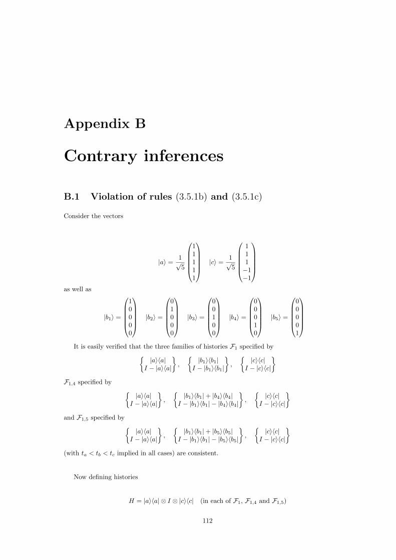
Appendix B
Contrary inferences
B.1 Violation of rules (3.5.1b) and (3.5.1c)
Consider the vectors
|a〉 =1√5
11111
|c〉 =1√5
111−1−1
as well as
|b1〉 =
10000
|b2〉 =
01000
|b3〉 =
00100
|b4〉 =
00010
|b5〉 =
00001
It is easily verified that the three families of histories F1 specified by
|a〉〈a|I − |a〉〈a|
,
|b1〉〈b1|
I − |b1〉〈b1|
,
|c〉〈c|
I − |c〉〈c|
F1,4 specified by
|a〉〈a|I − |a〉〈a|
,
|b1〉〈b1|+ |b4〉〈b4|
I − |b1〉〈b1| − |b4〉〈b4|
,
|c〉〈c|
I − |c〉〈c|
and F1,5 specified by
|a〉〈a|I − |a〉〈a|
,
|b1〉〈b1|+ |b5〉〈b5|
I − |b1〉〈b1| − |b5〉〈b5|
,
|c〉〈c|
I − |c〉〈c|
(with ta < tb < tc implied in all cases) are consistent.
Now defining histories
H = |a〉〈a| ⊗ I ⊗ |c〉〈c| (in each of F1, F1,4 and F1,5)
112

B1 = |a〉〈a| ⊗ |b1〉〈b1| ⊗ |c〉〈c| (in F1)
B1,4 = |a〉〈a| ⊗ (|b1〉〈b1|+ |b4〉〈b4|)⊗ |c〉〈c| (in F1,4)
B1,5 = |a〉〈a| ⊗ (|b1〉〈b1|+ |b5〉〈b5|)⊗ |c〉〈c| (in F1,5)
We obtain the following chain operators:
H =1
5|a〉〈c| B1 =
1
5|a〉〈c| B1,4 = 0 B1,5 = 0
(H⇒ B1) = I (H⇒ B1,4) = 0 (H⇒ B1,5) = 0
leading to probabilities
P (H ⇒ B1) = 1 (in F1) P (H ⇒ B1,4) = 0 (in F1,4) P (H ⇒ B1,5) = 0 (in F1,5)
Now
(H ⇒ B1,4) ∧ (H ⇒ B1,5) = (H ⇒ B1)
violating (3.5.1b) and
(H ⇒ B1,4) ∨ (H ⇒ B1) = (H ⇒ B1,4)
violating (3.5.1c), as required.
113

Bibliography
[1] S. Abramsky. High-level methods for quantum computation and information. ArXiv e-prints,
October 2009, 0910.3920.
[2] S. Abramsky. No-cloning in categorical quantum mechanics. ArXiv e-prints, October 2009,
0910.2401.
[3] S. Abramsky and A. Brandenburger. The sheaf-theoretic structure of non-locality and contex-
tuality. ArXiv e-prints, February 2011, 1102.0264.
[4] S. Abramsky and B. Coecke. A categorical semantics of quantum protocols. ArXiv e-prints,
February 2004, quant-ph/0402130.
[5] S. Abramsky and B. Coecke. Categorical quantum mechanics. ArXiv e-prints, August 2008,
0808.1023.
[6] S. Abramsky and R. Duncan. A categorical quantum logic. ArXiv e-prints, December 2005,
quant-ph/0512114.
[7] J. B. Altepeter, D. Branning, E. Jeffrey, T. C. Wei, P. G. Kwiat, R. T. Thew, J. L. O’Brien,
M. A. Nielsen, and A. G. White. Ancilla-assisted quantum process tomography. Physical
Review Letters, 90(19):193601, May 2003.
[8] C. Anastopoulos. Decoherence and classical predictability of phase-space histories. Physical
Review E, 53:4711–4722, May 1996.
[9] C. Anastopoulos. On the selection of preferred consistent sets. ArXiv e-prints, September
1997, quant-ph/9709051.
[10] C. Anastopoulos. Frequently asked questions about decoherence. International Journal of
Theoretical Physics, 41:1573–1590, 2002.
[11] A. Aspect, P. Grangier, and G. Roger. Experimental tests of realistic local theories via Bell’s
theorem. Phys. Rev. Lett., 47:460–463, Aug 1981.
114

[12] A. Bassi and G. Ghirardi. Can the decoherent histories description of reality be considered
satisfactory? Physics Letters A, 257:247–263, July 1999, gr-qc/9811050.
[13] A. Bassi and G. Ghirardi. About the notion of truth in the decoherent histories approach: A
reply to Griffiths. Physics Letters A, 265:153–155, January 2000, quant-ph/9912065.
[14] A. Bassi and G. Ghirardi. Decoherent histories and realism. Journal of Statistical Physics,
98:457–494, 2000. 10.1023/A:1018647510799.
[15] J. S. Bell. On the Einstein-Podolsky-Rosen paradox. Physics, 1(3):195–200, 1964.
[16] J. S. Bell. Speakable and unspeakable in quantum mechanics. Collected papers on quantum
philosophy. Cambridge Univ. Press, Cambridge, 1987.
[17] C. H. Bennett, G. Brassard, C. Crepeau, R. Jozsa, A. Peres, and W. K. Wootters. Teleporting
an unknown quantum state via dual classical and Einstein-Podolsky-Rosen channels. Physical
Review Letters, 70(13):1895–1899, Mar 1993.
[18] J. A. Bergou, U. Herzog, and M. Hillery. 11. Discrimination of Quantum States. In M. Paris
and J. Rehacek, editors, Quantum State Estimation, volume 649 of Lecture Notes in Physics,
pages 417–465. Springer Berlin / Heidelberg, 2004.
[19] J. A. Bergou, U. Herzog, and M. Hillery. Optimal unambiguous filtering of a quantum state:
An instance in mixed state discrimination. Physical Review A, 71(4):042314, Apr 2005.
[20] J. A. Bergou and M. Hillery. Universal programmable quantum state discriminator that is
optimal for unambiguously distinguishing between unknown states. Physical Review Letters,
94(16):160501, Apr 2005.
[21] G. Blaylock. The EPR paradox, Bell’s inequality, and the question of locality. American
Journal of Physics, 78:111–120, January 2010, 0902.3827.
[22] R. F. Blute, I. T. Ivanov, and P. Panangaden. Decoherent histories on graphs. ArXiv e-prints,
November 2001, gr-qc/0111020.
[23] R. F. Blute, I. T. Ivanov, and P. Panangaden. Discrete quantum causal dynamics. International
Journal of Theoretical Physics, 42:2025–2041, 2003. 10.1023/A:1027335119549.
[24] A. W. Bosse and J. B. Hartle. Representations of spacetime alternatives and their classical
limits. Physical Review A, 72(2):022105, August 2005, quant-ph/0503182.
[25] T. A. Brun. The Decoherence of Phase Space Histories. ArXiv e-prints, April 1994, gr-
qc/9404021.
115

[26] T. A. Brun. Quantum jumps as decoherent histories. Physical Review Letters, 78:1833–1837,
March 1997, quant-ph/9606025.
[27] T. A. Brun. Continuous measurements, quantum trajectories, and decoherent histories. Phys-
ical Review A, 61:042107, Mar 2000.
[28] T. A. Brun. Probability in decoherent histories. ArXiv e-prints, February 2003, quant-
ph/0302034.
[29] T. A. Brun and J. B. Hartle. Entropy of classical histories. Physical Review E, 59:6370–6380,
June 1999, quant-ph/9808024.
[30] J. Butterfield and C. J. Isham. Topos perspective on the Kochen-Specker theorem:
IV. Interval valuations. International Journal of Theoretical Physics, 41:613–639, 2002.
10.1023/A:1015276209768.
[31] A. Cabello, J. M. Estebaranz, and G. Garcıa-Alcaine. Bell-Kochen-Specker theorem: A proof
with 18 vectors. Physics Letters A, 212:183–187, February 1996, quant-ph/9706009.
[32] E. Calzetta and B. L. Hu. Decoherence of correlation histories. ArXiv e-prints, 1993, gr-
qc/9302013.
[33] C. M. Caves. Quantum mechanics of measurements distributed in time. A path-integral for-
mulation. Physical Review D, 33:1643–1665, Mar 1986.
[34] N. J. Cerf. Quantum cloning and the capacity of the Pauli channel. Physical Review Letters,
84:4497, 2000, quant-ph/9803058.
[35] A. Chefles. Quantum state discrimination. Contemporary Physics, 41(6):401–424, 2000.
[36] A. M. Childs, J. Preskill, and J. Renes. Quantum information and precision measurement.
Journal of Modern Optics, 47:155–176, 2000, quant-ph/9904021.
[37] G. Chiribella, G. M. D’Ariano, and P. Perinotti. Informational derivation of quantum theory.
Physical Review A, 84(1):012311, July 2011, 1011.6451.
[38] M.-D. Choi. Completely positive linear maps on complex matrices. Linear Algebra and its
Applications, 10(3):285 – 290, 1975.
[39] I. L. Chuang and M. A. Nielsen. Prescription for experimental determination of the dynamics
of a quantum black box. Journal of Modern Optics, 44(11-12):2455–2467, 1997.
[40] C. J. S. Clarke. The histories interpretation: Stability instead of consistency? ArXiv e-prints,
August 2000, quant-ph/0008060.
116

[41] B. Coecke. Quantum picturalism. Contemporary Physics, 51:59–83, January 2010, 0908.1787.
[42] B. Coecke and D. Pavlovic. Quantum measurements without sums. ArXiv e-prints, August
2006, quant-ph/0608035.
[43] O. Cohen. Pre- and postselected quantum systems, counterfactual measurements, and consis-
tent histories. Physical Review A, 51:4373–4380, Jun 1995.
[44] D. Craig, F. Dowker, J. Henson, S. Major, D. Rideout, and R. D. Sorkin. A Bell inequality
analog in quantum measure theory. Journal of Physics A: Mathematical and General, 40:501–
523, January 2007, quant-ph/0605008.
[45] D. Craig and P. Singh. Consistent histories in quantum cosmology. Foundations of Physics,
41:371–379, March 2011, 1001.4311.
[46] G. M. D’Ariano, M. Paris, and M. Sacchi. 2. Quantum Tomographic Methods. In M. Paris
and J. Rehacek, editors, Quantum State Estimation, volume 649 of Lecture Notes in Physics,
pages 189–204. Springer Berlin / Heidelberg, 2004. 10.1007/978-3-540-44481-7-2.
[47] G. M. D’Ariano, M. G. A. Paris, and M. F. Sacchi. Quantum tomography. In P. W. Hawkes,
editor, Advances in Imaging and Electron Physics, volume 128, pages 205 – 308. Elsevier, 2003.
[48] B. d’Espagnat. Are there realistically interpretable local theories? Journal of Statistical
Physics, 56:747–766, 1989. 10.1007/BF01016778.
[49] B. S. DeWitt and N. Graham, editors. The Many-Worlds Interpretation of Quantum Mechan-
ics, 1973.
[50] D. Dieks. Consistent histories and relativistic invariance in the modal interpretation of quan-
tum mechanics. Physics Letters A, 265(5-6):317 – 325, 2000.
[51] L. Diosi. Unique family of consistent histories in the Caldeira-Leggett model. ArXiv e-prints,
1993, gr-qc/9304016.
[52] L. Diosi. On the maximum number of decoherent histories. Physics Letters A, 203:267–268,
February 1995, gr-qc/9409028.
[53] L. Diosi. Anomalies of weakened decoherence criteria for quantum histories. Physical Review
Letters, 92(17):170401, April 2004, quant-ph/0310181.
[54] L. Diosi, N. Gisin, J. Halliwell, and I. C. Percival. Decoherent histories and quantum state
diffusion. Physical Review Letters, 74:203–207, Jan 1995.
[55] A. Doring. Topos theory and ‘neo-realist’ quantum theory. ArXiv e-prints, December 2007,
0712.4003.
117

[56] A. Doring. Topos quantum logic and mixed states. ArXiv e-prints, April 2010, 1004.3561.
[57] A. Doring and C. J. Isham. A topos foundation for theories of physics: I. Formal languages
for physics. Journal of Mathematical Physics, 49(5):053515, May 2008, quant-ph/0703060.
[58] A. Doring and C. J. Isham. A topos foundation for theories of physics: II. Daseinisation and
the liberation of quantum theory. Journal of Mathematical Physics, 49(5):053516, May 2008,
quant-ph/0703062.
[59] A. Doring and C. J. Isham. A topos foundation for theories of physics: III. The representation
of physical quantities with arrows. Journal of Mathematical Physics, 49(5):053517, May 2008,
quant-ph/0703064.
[60] A. Doring and C. J. Isham. A topos foundation for theories of physics: IV. Categories of
systems. Journal of Mathematical Physics, 49(5):053518, May 2008, quant-ph/0703066.
[61] A. Doring and C. J. Isham. ‘What is a thing?’: topos theory in the foundations of physics.
ArXiv e-prints, March 2008, 0803.0417.
[62] A. Doring and C. J. Isham. Classical and quantum probabilities as truth values. Journal of
Mathematical Physics, 53(3):032101, March 2012, 1102.2213.
[63] A. Doring and R. Soares Barbosa. Unsharp values, domains and topoi. ArXiv e-prints, July
2011, 1107.1083.
[64] F. Dowker and Y. Ghazi-Tabatabai. The Kochen-Specker theorem revisited in quantum mea-
sure theory. Journal of Physics A: Mathematical and General, 41(10):105301, March 2008,
0711.0894.
[65] F. Dowker, S. Johnston, and R. D. Sorkin. Hilbert spaces from path integrals. Journal of
Physics A: Mathematical and General, 43(26):A265302, July 2010, 1002.0589.
[66] F. Dowker and A. Kent. Properties of consistent histories. Physical Review Letters,
75(17):3038–3041, Oct 1995.
[67] F. Dowker and A. Kent. On the consistent histories approach to quantum mechanics. Journal
of Statistical Physics, 82:1575–1646, 1996. 10.1007/BF02183396.
[68] R. Duncan. Types for quantum computing. PhD thesis, University of Oxford, 2006.
[69] I. L. Egusquiza and J. G. Muga. Consistent histories, the quantum Zeno effect, and time of
arrival. Physical Review A, 62(3):032103, September 2000, quant-ph/0003041.
[70] A. Einstein, B. Podolsky, and N. Rosen. Can quantum-mechanical description of physical
reality be considered complete? Physical Review, 47(10):777–780, May 1935.
118

[71] Y. C. Eldar, M. Stojnic, and B. Hassibi. Optimal quantum detectors for unambiguous detection
of mixed states. Physical Review A, 69(6):062318, Jun 2004.
[72] H. Everett III. The theory of the universal wave function. In B. S. DeWitt and N. Graham,
editors, The Many-Worlds Interpretation of Quantum Mechanics, page 3, 1973.
[73] E. Farhi and S. Gutmann. Analog analogue of a digital quantum computation. Physical Review
A, 57(4):2403–2406, Apr 1998.
[74] Y. Feng, R. Duan, and M. Ying. Unambiguous discrimination between mixed quantum states.
Physical Review A, 70(1):012308, Jul 2004.
[75] R. P. Feynman. Quantum Implications : Essays in Honour of David Bohm, chapter 13, pages
235–248. Routledge and Kegan Paul Ltd, London and New York, 1987.
[76] R. P. Feynman and A. R Hibbs. Quantum Mechanics and Path Integrals. New York: McGraw-
Hill, 1965.
[77] C. Flori. A topos formulation of history quantum theory. Journal of Mathematical Physics,
51(5):053527, 2010.
[78] C. Flori. Review of the topos approach to quantum theory. ArXiv e-prints, June 2011,
1106.5660.
[79] D. J. Foulis, R. J. Greechie, and G. T. Ruttimann. Filters and supports in orthoalgebras.
International Journal of Theoretical Physics, 31:789–807, 1992. 10.1007/BF00678545.
[80] S. J. Freedman and J. F. Clauser. Experimental test of local hidden-variable theories. Phys.
Rev. Lett., 28:938–941, Apr 1972.
[81] C. A. Fuchs, Rudiger Schack, and P. F. Scudo. De Finetti representation theorem for quantum-
process tomography. Physical Review A, 69(6):062305, Jun 2004.
[82] I. Gelfand and M. Naimark. On the imbedding of normed rings into the ring of operators in
Hilbert space. Rec. Math. [Mat. Sbornik] N. S., 12(54):197–213, 1943.
[83] M. Gell-Mann. Fundamental sources of unpredictability. Annals of the New York Academy of
Sciences, 879(1):1–7, 1999.
[84] M. Gell-Mann. Consciousness, reduction, and emergence. Annals of the New York Academy
of Sciences, 929(1):41–49, 2001.
[85] M. Gell-Mann and J. B. Hartle. Quantum mechanics in the light of quantum cosmology. In
Proc. 3rd Int. Symp. Foundations of Quantum Mechanics, Tokyo, pages 321–343, 1989.
119
[86] M. Gell-Mann and J. B. Hartle. Alternative decohering histories in quantum mechanics. In
K. K. Phua & Y. Yamaguchi, editor, High Energy Physics, pages 1303–1310, 1991.
[87] M. Gell-Mann and J. B. Hartle. Time symmetry and asymmetry in quantum mechanics and
quantum cosmology. ArXiv e-prints, 1991, gr-qc/9304023.
[88] M. Gell-Mann and J. B. Hartle. Classical equations for quantum systems. Physical Review,
D47:3345–3382, 1993, gr-qc/9210010.
[89] M. Gell-Mann and J. B. Hartle. Equivalent sets of histories and multiple quasiclassical domains.
ArXiv e-prints, 1994, gr-qc/9404013.
[90] M. Gell-Mann and J. B. Hartle. Strong decoherence. ArXiv e-prints, 1995, gr-qc/9509054.
[91] M. Gell-Mann and J. B. Hartle. Quasiclassical coarse graining and thermodynamic entropy.
Physical Review, A76:022104, 2007, quant-ph/0609190. Dedicated to Rafael Sorkin on his 60th
birthday.
[92] M. Gell-Mann and J. B. Hartle. Decoherent histories quantum mechanics with one ’real’
fine-grained history. ArXiv e-prints, 2011, 1106.0767.
[93] V. Gheorghiu and R. B. Griffiths. Separable operations on pure states. Physical Review A,
78(2):020304, August 2008, 0807.2360.
[94] N. Gisin. On the impossibility of covariant nonlocal “hidden” variables in quantum physics.
ArXiv e-prints, February 2010, 1002.1390.
[95] A. Gleason. Measures on the closed subspaces of a Hilbert space. Indiana University Mathe-
matics Journal, 6:885–893, 1957.
[96] S. Goldstein and D. N. Page. Linearly positive histories: Probabilities for a robust family of se-
quences of quantum events. Physical Review Letters, 74:3715–3719, May 1995, gr-qc/9403055.
[97] R. B. Griffiths. Consistent histories and the interpretation of quantum mechanics. Journal of
Statistical Physics, 36:219–272, 1984. 10.1007/BF01015734.
[98] R. B. Griffiths. Correlations in separated quantum systems: A consistent history analysis of
the epr problem. American Journal of Physics, 55(1):11–17, 1987.
[99] R. B. Griffiths. The consistency of consistent histories: A reply to d’Espagnat. Foundations
of Physics, 23:1601–1610, 1993. 10.1007/BF00732367.
[100] R. B. Griffiths. Consistent interpretation of quantum mechanics using quantum trajectories.
Physical Review Letters, 70(15):2201–2204, Apr 1993.
120

[101] R. B. Griffiths. Consistent quantum reasoning. ArXiv e-prints, May 1995, quant-ph/9505009.
[102] R. B. Griffiths. Review of R. Omnes, ‘The Interpretation of Quantum Mechanics’. ArXiv
e-prints, May 1995, quant-ph/9505008.
[103] R. B. Griffiths. Consistent histories and quantum reasoning. Physical Review A, 54(4):2759–
2774, Oct 1996.
[104] R. B. Griffiths. Choice of consistent family, and quantum incompatibility. Physical Review A,
57:1604–1618, Mar 1998.
[105] R. B. Griffiths. Consistent histories and quantum delayed choice. Fortschritte der Physik,
46:741–748, 1998, quant-ph/9810016.
[106] R. B. Griffiths. Bohmian mechanics and consistent histories. Physics Letters A, 261:227–234,
October 1999, quant-ph/9902059.
[107] R. B. Griffiths. Consistent quantum counterfactuals. Physical Review A, 60:R5–R8, Jul 1999.
[108] R. B. Griffiths. Consistent histories, quantum truth functionals, and hidden variables. Physics
Letters A, 265(1-2):12 – 19, 2000.
[109] R. B. Griffiths. Consistent quantum realism: A reply to Bassi and Ghirardi. ArXiv e-prints,
January 2000, quant-ph/0001093.
[110] R. B. Griffiths. Consistent Quantum Theory. Cambridge University Press, 2002.
[111] R. B. Griffiths. Consistent resolution of some relativistic quantum paradoxes. Physical Review
A, 66(6):062101, Dec 2002.
[112] R. B. Griffiths. Nature and location of quantum information. Physical Review A, 66(1):012311,
July 2002, quant-ph/0203058.
[113] R. B. Griffiths. Probabilities and quantum reality: Are there correlata? ArXiv e-prints,
September 2002, quant-ph/0209116.
[114] R. B. Griffiths. Quantum mechanics without measurements. ArXiv e-prints, December 2006,
quant-ph/0612065.
[115] R. B. Griffiths. Types of quantum information. Physical Review A, 76(6):062320, December
2007, 0707.3752.
[116] R. B. Griffiths. A consistent quantum ontology. ArXiv e-prints, May 2011, 1105.3932.
[117] R. B. Griffiths. EPR, Bell, and quantum locality. American Journal of Physics, 79:954–965,
September 2011, 1007.4281.
121

[118] R. B. Griffiths. Quantum locality. Foundations of Physics, 41:705–733, 2011. 10.1007/s10701-
010-9512-5.
[119] R. B. Griffiths. The logic of consistent histories: A reply to Maudlin. ArXiv e-prints, October
2011, 1110.0974.
[120] R. B. Griffiths. Hilbert space quantum mechanics is noncontextual. ArXiv e-prints, January
2012, 1201.1510.
[121] R. B. Griffiths. Quantum counterfactuals and locality. ArXiv e-prints, December 2012,
1201.0255.
[122] R. B. Griffiths and J. B. Hartle. Comment on “Consistent sets yield contrary inferences in
quantum theory”. Physical Review Letters, 81:1981, August 1998, gr-qc/9710025.
[123] R. B. Griffiths and R. Omnes. Consistent histories and quantum measurements. Physics
Today, 52(8):26–31, 1999.
[124] R. B. Griffiths, S. Wu, L. Yu, and S. M. Cohen. Atemporal diagrams for quantum circuits.
Physical Review A, 73(5):052309, May 2006, quant-ph/0507215.
[125] J. J. Halliwell. Smeared Wigner functions and quantum-mechanical histories. Physical Review
D, 46:1610–1615, Aug 1992.
[126] J. J. Halliwell. Aspects of the decoherent histories approach to quantum mechanics. ArXiv
e-prints, August 1993, gr-qc/9308005.
[127] J. J. Halliwell. A review of the decoherent histories approach to quantum mechanics. Annals
of the New York Academy of Sciences, 755:726–740, 1995, gr-qc/9407040.
[128] J. J. Halliwell. Decoherent histories and hydrodynamic equations. Physical Review D,
58(10):105015, November 1998, quant-ph/9805062.
[129] J. J. Halliwell. Decoherent histories and the emergent classicality of local densities. Physical
Review Letters, 83:2481–2485, September 1999, quant-ph/9905094.
[130] J. J. Halliwell. Effective theories of coupled classical and quantum variables. In H.-P. Breuer
& F. Petruccione, editor, Lecture Notes in Physics, Berlin Springer Verlag, volume 526 of
Lecture Notes in Physics, Berlin Springer Verlag, page 153, 1999, gr-qc/9808071.
[131] J. J. Halliwell. The emergence of hydrodynamic equations from quantum theory: A decoherent
histories analysis. ArXiv e-prints, 1999, quant-ph/9912037.
[132] J. J. Halliwell. Somewhere in the universe: Where is the information stored when histories
decohere? Physical Review D, 60(10):105031, November 1999, quant-ph/9902008.
122

[133] J. J. Halliwell. Approximate decoherence of histories and ‘t Hooft’s deterministic quantum
theory. Physical Review D, 63(8):085013, April 2001, quant-ph/0011103.
[134] J. J. Halliwell. Decoherent histories for spacetime domains. In J. G. Muga, R. S. Mayato, &
I. L. Egusquiza, editor, Time in Quantum Mechanics, page 153, 2002, quant-ph/0101099.
[135] J. J. Halliwell. Some recent developments in the decoherent histories approach to quantum
theory. In Decoherence and Entropy in Complex Systems, volume 633 of Lecture Notes in
Physics, pages 63–83. Springer Berlin / Heidelberg, 2004. 10.1007/978-3-540-40968-7-5.
[136] J. J. Halliwell. Macroscopic superpositions, decoherent histories and the emergence of hydro-
dynamic behaviour. ArXiv e-prints, March 2009, 0903.1802.
[137] J. J. Halliwell. Partial decoherence of histories and the Diosi test. ArXiv e-prints, April 2009,
0904.4388.
[138] J. J. Halliwell. Probabilities in quantum cosmological models: A decoherent histories analysis
using a complex potential. Physical Review D, 80(12):124032, December 2009, 0909.2597.
[139] J. J. Halliwell and J. Thorwart. Decoherent histories analysis of the relativistic particle.
Physical Review D, 64(12):124018, December 2001, gr-qc/0106095.
[140] J. J. Halliwell and P. Wallden. Invariant class operators in the decoherent histories analysis
of timeless quantum theories. Physical Review D, 73(2):024011, January 2006, gr-qc/0509013.
[141] J. J. Halliwell and J. M. Yearsley. Arrival times, complex potentials and decoherent histories.
Physical Review A, 79:062101, 2009.
[142] J. J. Halliwell and J. M. Yearsley. Quantum arrival time formula from decoherent histories.
Physics Letters A, 374:154–157, December 2009, 0903.1958.
[143] J. J. Halliwell and E. Zafiris. Decoherent histories approach to the arrival time problem.
Physical Review D, 57:3351–3364, March 1998, quant-ph/9706045.
[144] J. Hamilton, C. J. Isham, and J. Butterfield. A topos perspective on the Kochen-Specker
theorem: III. Von Neumann algebras as the base category. International Journal of Theoretical
Physics, 39:1413–1436, 2000. 10.1023/A:1003667607842.
[145] Y. D. Han, W. Y. Hwang, and I. G. Koh. Explicit solutions for negative-probability measures
for all entangled states. Physics Letters A, 221(5):283 – 286, 1996.
[146] J. B. Hartle. Spacetime coarse grainings in nonrelativistic quantum mechanics. Physical Review
D, 44:3173–3196, Nov 1991.
123

[147] J. B. Hartle. Spacetime quantum mechanics and the quantum mechanics of spacetime. ArXiv
e-prints, 1992, gr-qc/9304006.
[148] J. B. Hartle. The reduction of the state vector and limitations on measurement in the quantum
mechanics of closed systems. In B. L. Hu and T. A. Jacobson, editors, Directions in General
Relativity: Papers in Honor of Dieter Brill, Volume 2, page 129, 1993, gr-qc/9301011.
[149] J. B. Hartle. The quantum mechanics of closed systems. In R. J. Gleiser, C. N. Kozameh,
and O. M. Moreschi, editors, General Relativity and Gravitation 1992, page 81, 1993, gr-
qc/9210006.
[150] J. B. Hartle. The spacetime approach to quantum mechanics. Vistas in Astronomy, 37:569–
583, 1993, gr-qc/9210004.
[151] J. B. Hartle. Quasiclassical realms in a quantum universe. ArXiv e-prints, April 1994, gr-
qc/9404017.
[152] J. B. Hartle. Unitarity and causality in generalized quantum mechanics for nonchronal space-
times. Physical Review, D49:6543–6555, 1994, gr-qc/9309012.
[153] J. B. Hartle. Spacetime information. Physical Review, D51:1800–1817, 1995, gr-qc/9409005.
[154] J. B. Hartle. Quantum cosmology: Problems for the 21st century. ArXiv e-prints, 1997,
gr-qc/9701022. To appear in ’Physics 2001’, edited by M. Kumar.
[155] J. B. Hartle. Theories of everything and Hawking’s wave function of the universe. ArXiv
e-prints, pages 38–50, 2002, gr-qc/0209047. To appear in ‘The Future of Theoretical Physics
and Cosmology’, Stephen Hawking 60th Birthday Symposium, Cambridge Univ. Press.
[156] J. B. Hartle. What Connects Different Interpretations of Quantum Mechanics? ArXiv e-prints,
May 2003, quant-ph/0305089.
[157] J. B. Hartle. Bohmian histories and decoherent histories. Physical Review A, 69:042111, Apr
2004.
[158] J. B. Hartle. Linear positivity and virtual probability. Physical Review A, 70(2):022104,
August 2004, quant-ph/0401108.
[159] J. B. Hartle. The physics of now. American Journal of Physics, 73:101–109, February 2005,
gr-qc/0403001.
[160] J. B. Hartle. Glafka 2004: Generalizing quantum mechanics for quantum gravity. International
Journal of Theoretical Physics, 45:1390–1396, September 2006, gr-qc/0510126.
124

[161] J. B. Hartle. Quantum physics and human language. Journal of Physics A Mathematical
General, 40:3101–3121, March 2007, arXiv:quant-ph/0610131.
[162] J. B. Hartle. Quantum mechanics with extended probabilities. ArXiv e-prints, 2008, 0801.0688.
[163] J. B. Hartle. Quasiclassical realms. In Many Worlds: Everett, Quantum Theory, and Reality,
chapter 2, pages 73–98. Oxford University Press, 2010.
[164] J. B. Hartle and S. W. Hawking. Wave function of the universe. Physical Review D, 28:2960–
2975, Dec 1983.
[165] J. B. Hartle, R. Laflamme, and D. Marolf. Conservation laws in the quantum mechanics of
closed systems. Physical Review D, 51:7007–7016, June 1995, gr-qc/9410006.
[166] J. B. Hartle and D. Marolf. Comparing formulations of generalized quantum mechanics for
reparametrization-invariant systems. Physical Review D, 56:6247–6257, Nov 1997.
[167] W. Heisenberg. Uber den anschaulichen Inhalt der quantentheoretischen Kinematik und
Mechanik. Zeitschrift fur Physik, 43, 1927.
[168] C. W. Helstrom. Quantum detection and estimation theory. Journal of Statistical Physics,
1:231–252, 1969. 10.1007/BF01007479.
[169] U. Herzog and J. A. Bergou. Distinguishing mixed quantum states: Minimum-error discrim-
ination versus optimum unambiguous discrimination. Physical Review A, 70(2):022302, Aug
2004.
[170] U. Herzog and J. A. Bergou. Optimum unambiguous discrimination of two mixed quantum
states. Physical Review A, 71(5):050301, May 2005.
[171] B. J. Hiley and O. J. E. Maroney. Consistent histories and the Bohm approach. ArXiv e-prints,
September 2000, quant-ph/0009056.
[172] P. C. Hohenberg. Colloquium: An introduction to consistent quantum theory. Reviews of
Modern Physics, 82:2835–2844, October 2010, 0909.2359.
[173] A. Holevo. Statistical problems in quantum physics. In G. Maruyama and Yu. Prokhorov,
editors, Proceedings of the Second Japan-USSR Symposium on Probability Theory, volume
330 of Lecture Notes in Mathematics, pages 104–119. Springer Berlin / Heidelberg, 1973.
10.1007/BFb0061483.
[174] C. J. Isham. Canonical quantum gravity and the problem of time. ArXiv e-prints, 1992,
gr-qc/9210011.
125

[175] C. J. Isham. Quantum logic and the histories approach to quantum theory. Journal of
Mathematical Physics, 35:2157–2185, 1994, gr-qc/9308006.
[176] C. J. Isham. Quantum logic and decohering histories. ArXiv e-prints, 1995, quant-ph/9506028.
[177] C. J. Isham. Structural issues in quantum gravity. ArXiv e-prints, 1995, gr-qc/9510063.
[178] C. J. Isham. Topos theory and consistent histories: The internal logic of the set of all consistent
sets. International Journal of Theoretical Physics, 36:785–814, 1997. 10.1007/BF02435786.
[179] C. J. Isham. Topos methods in the foundations of physics. ArXiv e-prints, April 2010,
1004.3564.
[180] C. J. Isham and J. J. Butterfield. A topos perspective on the Kochen-Specker theorem: I.
Quantum states as generalized valuations. ArXiv e-prints, March 1998, quant-ph/9803055.
[181] C. J. Isham and J. J. Butterfield. A topos perspective on the Kochen-Specker theorem: II.
Conceptual aspects, and classical analogues. ArXiv e-prints, August 1998, quant-ph/9808067.
[182] C. J. Isham and N. Linden. Quantum temporal logic and decoherence functionals in the
histories approach to generalized quantum theory. Journal of Mathematical Physics, 35:5452–
5476, 1994, gr-qc/9405029.
[183] C. J. Isham and N. Linden. Information entropy and the space of decoherence functions in
generalized quantum theory. Physical Review A, 55(6):4030–4040, Jun 1997.
[184] C. J. Isham, N. Linden, K. Savvidou, and S. Schreckenberg. Continuous time and consistent
histories. Journal of Mathematical Physics, 39:1818–1834, April 1998, quant-ph/9711031.
[185] C. J. Isham, N. Linden, and S. Schreckenberg. The classification of decoherence functionals:
An analog of Gleason’s theorem. Journal of Mathematical Physics, 35:6360–6370, December
1994, arXiv:gr-qc/9406015.
[186] T. F. Jordan and E. D. Chisolm. Probability sum rules and consistent quantum histories.
Physics Letters A, 373:3016–3020, August 2009, 0801.2725.
[187] R. E. Kastner. Weak values and consistent histories in quantum theory. ArXiv e-prints, July
2002, quant-ph/0207182.
[188] A. Kent. Remarks on ‘Consistent histories and Bohmian mechanics’. ArXiv e-prints, November
1995, quant-ph/9511032.
[189] A. Kent. Quasiclassical dynamics in a closed quantum system. Physical Review A, 54:4670–
4675, Dec 1996.
126

[190] A. Kent. Consistent sets yield contrary inferences in quantum theory. Physical Review Letters,
78(15):2874–2877, Apr 1997.
[191] A. Kent. Quantum histories. Physica Scripta Volume T, 76:78–84, 1998, gr-qc/9809026.
[192] S. Kochen and E. P. Specker. The problem of hidden variables in quantum mechanics. Journal
Of Mathematics and Mechanics, 17(1):59–87, 1967.
[193] A. Kuah, K. Modi, C. A. Rodrıguez-Rosario, and E. C. G. Sudarshan. How state preparation
can affect a quantum experiment: Quantum process tomography for open systems. Physical
Review A, 76(4):042113, Oct 2007.
[194] F. Laloe. Do we really understand quantum mechanics? Strange correlations, paradoxes, and
theorems. American Journal of Physics, 69:655–701, June 2001.
[195] S. Lloyd. Decoherent histories and generalized measurements. ArXiv e-prints, April 2005,
quant-ph/0504155.
[196] X. Martin, D. O’Connor, and R. D. Sorkin. Random walk in generalized quantum theory.
Physical Review D, 71:024029, Jan 2005.
[197] T. Maudlin. What Bell proved: A reply to Blaylock. American Journal of Physics, 78:121–125,
January 2010.
[198] T. Maudlin. How Bell reasoned: A reply to Griffiths. American Journal of Physics, 79(9):966–
970, 2011.
[199] J. N. McElwaine. Approximate and exact consistency of histories. Physical Review A, 53:2021–
2032, April 1996, quant-ph/9506034.
[200] J. Mimih and M. Hillery. Unambiguous discrimination of special sets of multipartite states
using local measurements and classical communication. Physical Review A, 71(1):012329, Jan
2005.
[201] M. Mohseni, A. T. Rezakhani, and D. A. Lidar. Quantum-process tomography: Resource
analysis of different strategies. Physical Review A, 77(3):032322, Mar 2008.
[202] M. Mohseni, A. M. Steinberg, and J. A. Bergou. Optical realization of optimal unambiguous
discrimination for pure and mixed quantum states. Physical Review Letters, 93(20):200403,
Nov 2004.
[203] T. Muller. Branch dependence in the consistent histories approach to quantum mechanics.
ArXiv e-prints, 2005, quant-ph/0506051.
127

[204] M. A. Nielsen and I. L. Chuang. Quantum Computation and Quantum Information (Cambridge
Series on Information and the Natural Sciences). Cambridge University Press, 1 edition,
January 2004.
[205] D. Noltingk. A Consistent Histories approach to the Unruh effect. ArXiv e-prints, May 2000,
gr-qc/0005063.
[206] R. Omnes. The possible role of elementary particle physics in cosmology. Physics Reports,
3(1):1 – 55, 1972.
[207] R. Omnes. Logical reformulation of quantum mechanics. I. Foundations. Journal of Statistical
Physics, 53:893–932, 1988. 10.1007/BF01014230.
[208] R. Omnes. Logical reformulation of quantum mechanics. II. Interferences and the
Einstein-Podolsky-Rosen experiment. Journal of Statistical Physics, 53:933–955, 1988.
10.1007/BF01014231.
[209] R. Omnes. Logical reformulation of quantum mechanics. III. Classical limit and irreversibility.
Journal of Statistical Physics, 53:957–975, 1988. 10.1007/BF01014232.
[210] R. Omnes. Logical reformulation of quantum mechanics. IV. Projectors in semiclassical physics.
Journal of Statistical Physics, 57:357–382, 1989. 10.1007/BF01023649.
[211] R. Omnes. The Einstein-Podolsky-Rosen problem: A new solution. Physics Letters A, 138(4-
5):157 – 159, 1989.
[212] R. Omnes. From Hilbert space to common sense: A synthesis of recent progress in the inter-
pretation of quantum mechanics. Annals of Physics, 201(2):354 – 447, 1990.
[213] R. Omnes. About the notion of truth in quantum mechanics. Journal of Statistical Physics,
62:841–861, 1991. 10.1007/BF01017986.
[214] R. Omnes. Consistent interpretations of quantum mechanics. Reviews of Modern Physics,
64(2):339–382, Apr 1992.
[215] R. Omnes. A model for the uniqueness of data and decoherent histories. Physics Letters A,
187(1):26 – 30, 1994.
[216] R. Omnes. A new interpretation of quantum mechanics and its consequences in epistemology.
Foundations of Physics, 25:605–629, 1995. 10.1007/BF02059008.
[217] R. Omnes. General theory of the decoherence effect in quantum mechanics. Physical Review
A, 56:3383–3394, Nov 1997.
128

[218] R. Omnes. Theory of the decoherence effect. Fortschritte der Physik, 46(6-8):771–777, 1998.
[219] R. Omnes. Are there unsolved problems in the interpretation of quantum mechanics? In
Heinz-Peter Breuer and Francesco Petruccione, editors, Open Systems and Measurement in
Relativistic Quantum Theory, volume 526 of Lecture Notes in Physics, pages 169–194. Springer
Berlin / Heidelberg, 1999. 10.1007/BFb0104403.
[220] R. Omnes. Decoherence: An irreversible process. In P. Blanchard, E. Joos, D. Giulini,
C. Kiefer, and I.-O. Stamatescu, editors, Decoherence: Theoretical, Experimental, and Con-
ceptual Problems, volume 538 of Lecture Notes in Physics, pages 291–298. Springer Berlin /
Heidelberg, 2000. 10.1007/3-540-46657-6-24.
[221] R. Omnes. Quantum philosophy: Understanding and interpreting contemporary science.
American Journal of Physics, 69(1):94–95, 2001.
[222] R. Omnes. Decoherence, irreversibility, and selection by decoherence of exclusive quantum
states with definite probabilities. Physical Review A, 65:052119, May 2002.
[223] R. Omnes. Model of quantum reduction with decoherence. Physical Review D, 71(6):065011,
March 2005, quant-ph/0411201.
[224] R. Omnes. Decoherence and reduction. ArXiv e-prints, April 2006, quant-ph/0604130.
[225] R. Omnes. Possible agreement of wave function reduction from the basic principles of quantum
mechanics. ArXiv e-prints, December 2007, 0712.0730.
[226] R. Omnes. On the derivation of reduction from the Schrodinger equation. A disproof of no-go
theorems and a proposal. ArXiv e-prints, November 2009, 0911.0598.
[227] R. Omnes. On the derivation of wave function reduction from Schrodinger’s equation: A
model. ArXiv e-prints, June 2010, 1006.3227.
[228] R. Omnes. Decoherence and wave function collapse. Foundations of Physics, 41:1857–1880,
2011.
[229] V. Paulsen. Completely Bounded Maps and Operator Algebras. Cambridge University Press,
2003.
[230] J. P. Paz and W. H. Zurek. Environment-induced decoherence, classicality, and consistency of
quantum histories. Physical Review D, 48:2728–2738, Sep 1993.
[231] A. Peres and W. K. Wootters. Optimal detection of quantum information. Physical Review
Letters, 66(9):1119–1122, Mar 1991.
129

[232] D. Polarski. Primordial fluctuations from inflation: A consistent histories approach. Physics
Letters B, 446:53–57, January 1999, gr-qc/9812008.
[233] J. F. Poyatos, J. I. Cirac, and P. Zoller. Complete characterization of a quantum process: The
two-bit quantum gate. Physical Review Letters, 78:390–393, Jan 1997.
[234] S. Rahimi-Keshari, A. Scherer, A. Mann, A. T. Rezakhani, A. I. Lvovsky, and B. C. Sanders.
Quantum process tomography with coherent states. New Journal of Physics, 13(1):013006,
January 2011, 1009.3307.
[235] I. Raptis. Sheafifying consistent histories. ArXiv e-prints, July 2001, quant-ph/0107037.
[236] P. Raynal and N. Lutkenhaus. Optimal unambiguous state discrimination of two density
matrices: Lower bound and class of exact solutions. Physical Review A, 72(2):022342, Aug
2005.
[237] O. Rudolph. Consistent histories and operational quantum theory. International Journal of
Theoretical Physics, 35:1581–1636, August 1996, quant-ph/9512024.
[238] O. Rudolph. On the consistent effect histories approach to quantum mechanics. Journal of
Mathematical Physics, 37:5368–5379, November 1996, quant-ph/9605037.
[239] O. Rudolph. The representation theory of decoherence functionals in history quantum theories.
ArXiv e-prints, October 1998, math-ph/9810017.
[240] O. Rudolph and J. D. M. Wright. Homogeneous decoherence functionals in standard and
history quantum mechanics. Communications in Mathematical Physics, 204:249–267, 1999,
math-ph/9807024.
[241] K. Savvidou. Continuous time in consistent histories. ArXiv e-prints, December 1999, gr-
qc/9912076.
[242] A. Scherer and A. N. Soklakov. Decoherence properties of arbitrarily long histories. AIP
Conference Proceedings, 734(1):417–420, 2004.
[243] A. Scherer and A. N. Soklakov. Initial states and decoherence of histories. Journal of Mathe-
matical Physics, 46(4):042108, April 2005, quant-ph/0405080.
[244] A. Scherer, A. N. Soklakov, and R. Schack. A simple necessary decoherence condition for a
set of histories. Physics Letters A, 326:307–314, June 2004, quant-ph/0401132.
[245] I. E. Segal. Irreducible representations of operator algebras. Bull. Amer. Math. Soc., 53(2):73–
88, 1947.
130

[246] G. Segre. There exist consistent temporal logics admitting changes of History. ArXiv e-prints,
December 2006, gr-qc/0612021.
[247] E. Seidewitz. Consistent histories of systems and measurements in spacetime. Foundations of
Physics, 41:1163–1192, July 2011, 1002.3917.
[248] P. Selinger. Dagger compact closed categories and completely positive maps (extended ab-
stract). Electronic Notes in Theoretical Computer Science, 170(0):139 – 163, 2007.
[249] P. Selinger. Finite dimensional Hilbert spaces are complete for dagger compact closed cate-
gories (extended abstract). Electronic Notes in Theoretical Computer Science, 270(1):113 –
119, 2011.
[250] U. Sinha, C. Couteau, Z. Medendorp, I. Sollner, R. Laflamme, R. Sorkin, and G. Weihs. Testing
Born’s rule in quantum mechanics with a triple slit experiment. In L. Accardi, G. Adenier,
C. Fuchs, G. Jaeger, A. Y. Khrennikov, J.-A. Larsson, & S. Stenholm, editor, American
Institute of Physics Conference Series, volume 1101, pages 200–207, March 2009, 0811.2068.
[251] R. D. Sorkin. Quantum measure theory and its interpretation. ArXiv e-prints, July 1995,
gr-qc/9507057.
[252] R. D. Sorkin. An exercise in “anhomomorphic logic”. Journal of Physics Conference Series,
67(1):012018, May 2007, quant-ph/0703276.
[253] R. D. Sorkin. Quantum dynamics without the wavefunction. Journal of Physics A: Mathe-
matical and General, 40:3207–3221, March 2007, quant-ph/0610204.
[254] R. D. Sorkin. Logic is to the quantum as geometry is to gravity. ArXiv e-prints, April 2010,
1004.1226.
[255] R. D. Sorkin. Toward a “fundamental theorem of quantal measure theory”. ArXiv e-prints,
April 2011, 1104.0997.
[256] H. P. Stapp. Nonlocality, counterfactual, and consistent histories. ArXiv e-prints, May 1999,
quant-ph/9905055.
[257] E. C. G. Sudarshan and T. Rothman. A new interpretation of Bell’s inequalities. International
Journal of Theoretical Physics, 32:1077–1086, 1993. 10.1007/BF00671790.
[258] J. Twamley. Phase-space decoherence: a comparison between consistent histories and envi-
ronment induced superselection. Physical Review D, 48:5730, 1993.
[259] P. Wallden. Spacetime coarse grainings in the decoherent histories approach to quantum
theory. ArXiv e-prints, July 2006, gr-qc/0607072.
131

[260] P. Wallden. Quantum Zeno effect in the decoherent histories. Journal of Physics Conference
Series, 67(1):012043, May 2007, 0704.1551.
[261] P. Wallden. Spacetime coarse grainings and the problem of time in the decoherent histories
approach to quantum theory. International Journal of Theoretical Physics, 47:1512–1532,
2008. 10.1007/s10773-007-9592-y.
[262] G. Wang and M. Ying. Unambiguous discrimination among quantum operations. Physical
Review A, 73(4):042301, April 2006, quant-ph/0512142.
[263] G. Weihs, T. Jennewein, C. Simon, H. Weinfurter, and A. Zeilinger. Violation of Bell’s inequal-
ity under strict Einstein locality conditions. Physical Review Letters, 81:5039–5043, December
1998, arXiv:quant-ph/9810080.
[264] E. P. Wigner. The problem of measurement. American Journal of Physics, 31:6–15, January
1963.
[265] C. H. Woo. Consistent-histories description of a world of increasing entropy. ArXiv e-prints,
January 1999, quant-ph/9901055.
[266] X. Wu and K. Xu. Partial standard quantum process tomography. ArXiv e-prints, May 2011,
1105.2991.
[267] J. M. Yearsley. A review of the decoherent histories approach to the arrival time problem in
quantum theory. Journal of Physics Conference Series, 306(1):012056, 2011.
132