6

EUROPEAN ECONOMY

Economic and Financial Affairs

ISSN 2443-8022 (online)

EUROPEAN ECONOMY

The Relation between Productivity and Compensation in Europe

Paolo Pasimeni

DISCUSSION PAPER 079 | MARCH 2018

European Economy Discussion Papers are written by the staff of the European Commission’s Directorate-General for Economic and Financial Affairs, or by experts working in association with them, to inform discussion on economic policy and to stimulate debate. The views expressed in this document are solely those of the author(s) and do not necessarily represent the official views of the European Commission. Authorised for publication by José Leandro, Director for Policy, Strategy and Communication.

LEGAL NOTICE Neither the European Commission nor any person acting on behalf of the European Commission is responsible for the use that might be made of the information contained in this publication. This paper exists in English only and can be downloaded from https://ec.europa.eu/info/publications/economic-and-financial-affairs-publications_en. Luxembourg: Publications Office of the European Union, 2018 PDF ISBN 978-92-79-77416-4 ISSN 2443-8022 doi:10.2765/749614 KC-BD-18-006-EN-N

© European Union, 2018 Non-commercial reproduction is authorised provided the source is acknowledged. For any use or reproduction of material that is not under the EU copyright, permission must be sought directly from the copyright holders.

European Commission Directorate-General for Economic and Financial Affairs

The Relation between Productivity and Compensation in Europe Paolo Pasimeni Abstract One of the classical problems of political economy has been to understand the relation between labour compensation and labour productivity; in more recent years, then, wage growth has become a key concern for the conduct of monetary policy by major central banks. This paper studies to what extent increases in productivity translate into increases in compensations. While previous studies had investigated this relation in the case of the US, this work enlarges the scope of the analysis to a set of 34 advanced economies over the past half century. The results show on average a significant link between growth in productivity and growth in compensation, however there is no one-to-one relation, there is instead a significant gap. Cyclical conditions as well as labour market structures greatly affect this relation. These findings imply that policies aiming at increasing productivity are a necessary but not sufficient condition to achieve also appropriate pay growth, because other factors intervene to weaken the link between the two. Although this topic has gained more prominence in the US, the analysis shows that these findings apply to the EU and to other advanced economies as well. Finally, to the extent that the gap between productivity and compensation affects aggregate demand, understanding it is crucial for the conduct of macroeconomic policies. JEL Classification: D3; E24; E25; J3. Keywords: Productivity, compensation, wage share, labour market, employment, aggregate demand. Acknowledgements: The author is grateful to Eric Meyermans, Larry Mishel, Anna Stansbury, Mirco Tomasi, and Borek Vasicek for their useful comments. The opinions expressed in this paper are the author's alone and cannot be attributed to the institutions with which he is affiliated. Contact: Paolo Pasimeni, European Commission, Directorate-General for Economic and Financial Affairs, paolo.pasimeni@ec.europa.eu.

EUROPEAN ECONOMY Discussion Paper 079

CONTENTS

1. Introduction ..................................................................................................................................... 5

2. Data ...................................................................................................................................... 7

3. Empirical strategy ........................................................................................................................... 9

3.1. Baseline.................................................................................................................................................... 9

3.2. Alternative specifications ................................................................................................................... 10

4. Results .................................................................................................................................... 11

4.1. Full sample of 34 countries ................................................................................................................. 11

4.2. The EU..................................................................................................................................................... 12

4.3. The non-EU ............................................................................................................................................ 15

5. Implications ................................................................................................................................... 17

6. Conclusions ................................................................................................................................... 18

LIST OF TABLES

4.1. Changes in compensation and in productivity (full sample, full period, single years) .................................................................................................................................... 11

4.2. Changes in compensation and in productivity (EU 28, full period, single years) ............... 13

4.3. Changes in compensation and in productivity (panel, non EU countries, full period, single years) .................................................................................................................... 15

5.1. Current account balance and gap between compensation and productivity (full sample, full period, single years) ............................................................................................... 18

LIST OF GRAPHS

1.1. Adjusted wage share – Total economy – 1960-2016 ................................................................ 5

1.2. Real hourly compensation and productivity – 1970-2016 ....................................................... 6

4.1. Changes in compensation and in productivity (full sample, full period, alternative specifications) .............................................................................................................................. 12

4.2. Changes in compensation and in productivity (EU 28, full period, alternative specifications) .............................................................................................................................. 14

4.3. Changes in compensation and in productivity (EU 28, before and after EMU, single years) .................................................................................................................................. 15

4.4. Changes in compensation and in productivity in individual countries (non EU countries, full period, single years) ............................................................................................ 16

REFERENCES

ANNEX I - UNIT-ROOT TESTS

ANNEX II - TEST FOR PANEL-LEVEL HETEROSKEDASTICITY AND UTOCORRELATION

ANNEX III - DETAILED RESULTS OF THE ALTERNATIVE SPECIFICATIONS

4

1. INTRODUCTION

One of the classical problems of political economy has been to understand the distribution of income between factors of production (Smith, 1776; Ricardo, 1817; Marx, 1867-1883). The relation between labour compensation and labour productivity has been at the core of macroeconomic analysis, since it makes a link between incomes at the level of the household and incomes at the macroeconomic level (national accounts) (Atkinson, 2009). In more recent years, then, wage growth has become a key concern for the conduct of monetary policy by major central banks (Yellen, 2015; Draghi, 2017).

res of national income received by labour and capital were constant over the long run (Kaldor, 1957).

raph 1.1. Adjusted wage share – Total economy – 1960-2016

Denmark, Germany, Ireland, Spain, France, Italy, Netherlands, Portugal, Finland, Sweden, United Kingdom).

Source: AMECO.

grown over time, productivity has done it faster, leading in some cases to a considerable divergence.

Standard economic theory suggests that compensation's dynamics should reflect productivity's developments; the two should therefore grow together. Arguing that growth in real compensation should mirror growth in real productivity means that nominal unit labour costs should be driven just by the inflation rate, and therefore real unit labour costs should remain constant. But, given that real unit labour costs are another way to express the overall share of income accruing to labour, this condition implies that the labour income share in the economy should remain constant. This was in fact one of the so-called "Kaldor's fact", the idea that the sha

G

Note: Adjusted wage share: total economy: as percentage of GDP at current prices (Compensation per employee as percentage of GDP at market prices per person employed). Europe is an average of 12 countries for which the entire series since 1960 could be built (Belgium,

The observation of the trends in the labour income share over the past half century suggests that this assumption was wrong (Piketty and Saez, 2013): in nearly all advanced economies the functional distribution of income, in fact, has substantially changed, leading to a declining labour share since the 1970's (Karabarbouinis and Neiman, 2014) and in particular since the beginning of this millennium (ILO, 2015). This stylised fact is corroborated by the observation of the long-term trends in real compensation and real productivity: although they have both

5

The discussion on whether increases in productivity translate into increases in compensations or are instead decoupled has become prominent for economic policy making today (Council of Economic Advisers, 2014). A first key question is to understand to what extent the dynamics of compensations and productivity are linked, if there is a relation between the two and how strong this relation is. If there is any divergence, we should also try to understand how significant it is.

Graph 1.2. Real hourly compensation and productivity – 1970-2016

Note: Adjusted wage share: total economy: as percentage of GDP at current prices (Compensation per employee as percentage of GDP at market prices per person employed). Europe is an average of 12 countries for which the entire series since 1960 could be built (Belgium, Denmark, Germany, Ireland, Spain, France, Italy, Netherlands, Portugal, Finland, Sweden, United Kingdom).

Source: AMECO.

The decoupling between productivity growth and rise in compensation is noticeable in Japan and the US, less so in Europe; however several considerations are in order. First, these data refer to average compensation, while a considerable gap has developed between median and average compensation, leading to an even lower increase in compensation for the median; the gap is therefore underestimated almost everywhere. Second, data for Europe are an average of 12 countries for which the entire series since 1970 could be built, and this may mask some country-specific circumstances. Third, one of these specificities refers to the UK, where between 1996 and 2007 average compensation grew twice as fast as productivity, but this was driven by rising top compensations while the median was stagnating. Fourth, in this average for Europe, we can observe an almost perfect one-for-one linkage up until 1993, when the first considerable divergence shows up, and then a larger one staring after 2009 and growing at present time. This stylised illustration, however, is not enough to assert the existence of a perfect link, of a significant gap, or of a full decoupling between productivity and compensation.

If true, the decoupling between productivity and compensation may contribute to explaining the other major trend over the past decades, i.e. rising inequality. As such, failure to translate labour productivity gains into workers' welfare could arguably be one explanation for the missing "trickle down" effect observed over the past decades; of course, other factors too contribute to explaining the rise in inequality, such as policies for redistribution.

This phenomenon has attracted greater attention in the US, where recent analyses have tried to describe it (Fleck et al, 2011) and to investigate its causes. Mishel and Bernstein (1994) first raised concerns about deteriorating wages for "working America", which were primary responsible for slow growth and widening inequality. Feldstein (2008), however, did not find evidence of a decoupling between productivity and compensation in the US over the previous half century, when accounting for non-wage benefits and using the same product price deflator for the two series. Deflating both productivity and compensation by the same deflator, as Feldstein (2008) suggests, may look reasonable from the point of view of studying the relative functional distribution of income. However,

6

if one wants to understand to what extent productivity growth translates into better living standards for workers, it is probably more appropriate to build the measure of real compensation by using a consumer price deflator (IMF, 2017; Stansbury and Summers, 2017), as we do in this work.

Lawrence (2016) argues that the so-called historic divergence did not occur, if one accounts for depreciation of productivity, while an important divergence did materialise between wages and total compensation, due to the increasing share of non-wage compensation. Bivens and Mishel (2015) instead document the wedge between productivity and compensation growth in the US, starting in the 1970's, and find that growing inequality explains most of it, while individual productivity does not. The key difference between Bivens and Mishel (2015) on one side and Feldstein (2008) and Lawrence (2016) on the other is that they use slightly different concepts of labour compensations: the latter use average compensation, while the former look at median or production/non-supervisory compensation, therefore accounting for inequalities within the distribution of wages.

The recent work by Stansbury and Summers (2017) then uses all three measures: average, median, and production/non-supervisory compensation. They find that "a one percentage point increase in the rate of productivity growth has been associated with an increase in compensation growth of 0.7 to 1 percentage points for the median worker and for average compensation over 1973-2016, and of 0.4 to 0.7 percentage points for the average production/nonsupervisory worker".

All these studies focus on the US; we analyse this phenomenon, instead, in a larger set of countries, by using a panel covering the past half century for 34 countries: the 28 Member States of the EU and other economies for which data are available and comparable, such as the US, Japan, Canada, Norway, Iceland, and Switzerland. This large panel allows us to estimate general patterns all over advanced economies and then to differentiate by regions, with a special focus on the EU.

The first question we try to answer in this analysis is whether the dynamics of compensations and productivity have been linked or not. In other words, we will try to understand to what extent productivity gains have translated into increases in compensations for workers. Then, we measure how much, if not all, of the productivity gains are transferred to increases in compensations. Finally, we measure the gap between compensation and productivity and try to study its implications on other macroeconomic variables.

2. DATA

In order to meaningfully compare productivity and compensation we must use data for real compensation and real productivity. Compensations are both a source of revenues for workers and a cost for firms; in the first case they largely determine the welfare of workers and in the second case they affect firm's decisions of allocation of factors of production. A crucial step in calculating real compensation, then, is the choice of the appropriate deflator: this depends on the function we are more interested in. If we are more concerned with the cost structure of firms, it would be more appropriate to compare real productivity with real compensation deflated using the same GDP deflator, as some have suggested (Feldstein, 2008). Conversely, if we want to primarily study the actual purchasing power and welfare of workers, compensation deflated with a consumer price index is a better measure to compare with real productivity (IMF, 2017). Thus, for our purposes, it is useful to take compensation deflated by private consumption, rather than for the GDP deflator, because what we are interested in is the real value of compensations for workers which determines their actual living standards.

7

However, one might object that the difference in the two deflators used could contribute to determining a difference in the two main series we want to compare, growth in real productivity and in real compensation, if a gap exist between the two. It must be noted, nevertheless, that if a difference exists between the two measurements, this difference is likely to remain constant over the time period, so it does not affect our final findings. Nevertheless, and as a robustness check for our results, we have calculated real compensation also by applying the GDP deflator, to check whether this gives different real data than by using a CPI-deflated series. The results show that the two methods yield virtually the

non-wage compensation: the relative importance on non-wage compensation has actually increased over the recent decades. For this reason, we use data of

ty and compensation per employed person; however, changes in the work patterns of employees may actually influence the relation, and

dentical results. This allows us to compare real compensation and productivity both per hours worked and per person employed, and to

about mismeasurement of the number of hours worked is netted out by using this number as denominator to build both series. Thus the results cannot be affected by any measurement issue in

n-supervisory workers, it is fairly reasonable to say that the actual gap between increases in productivity and pay

We compose a balanced panel of 34 countries, including the 28 current members of the EU and the US, Japan, Canada, Norway, Switzerland and Iceland, using annual data starting in 1970.

same results1, so the choice of the price deflator cannot affect our findings.

Once established the deflator to be used to calculate real compensation, it is important to find measures which include not just wage but also

real compensation, including non-wage benefits.

The next step in the calculation of the data for our analysis is to define at which level real compensation and real productivity are better compared. The AMECO dataset provides figures for real compensation per employee, total economy; and for real gross domestic product per person employed. These measures allow us to study the relation between productivi

they are not adequately captured by this measure.

A more precise measurement, then, would be based on compensation and productivity per hour worked, rather than per person employed. Therefore we calculate real hourly compensation by dividing the real compensation per employee by the average number of hours worked per person employed, and real hourly productivity in two ways: one method is by deflating nominal hourly GDP with the GDP deflator, the second one is by dividing real GDP by the total number of hours worked in the economy each year; both methods provide, as expected, i

test the robustness of our findings.

There is a usual preoccupation when the total number of hours worked is used as an indicator at aggregate level, due to possible mismeasurement. In our case, however, it is important to clarify that the same data of hours worked are used to calculate hourly productivity and hourly compensation, so any concern

those data.

We can build in this way a large dataset covering all 28 EU countries plus the USA, Canada, Japan, Norway, Iceland and Switzerland, for a period of almost half a century, from 1970 to 2017. The fact that we use data for "average" compensation in total economy, and cannot compare them with more detailed data about the "median" compensation, nor with non-supervisory workers only, as some of the analyses applied to the case of the US do, implies that our findings will overestimate the increase in real compensation. In other words, given the existing divergence between "average" and "median" compensation growth, and the one between compensation of supervisory and no

growth for the median non-supervisory worker is larger than what our results will show.

1 The two series calculated with the two different deflators are strongly correlated: in the case of the US the correlation coefficient is: 99.8%; Italy: 99.5%; France: 99.9%; Germany: 99.7%; UK: 99.8%; Spain: 99.3%; Japan: 99.2%: Canada: 97.1%.

8

3. EMPIRICAL STRATEGY 3.1. BASELINE

We estimate a mode productivity:

st advanced economies were very different across the past five

g change) in hours worked per person employed as a control; the model be

specific effect of euro area membership on the relation between productivity and compensations.

The full specification of the

In all specifications we use robust standard errors.

l of changes in real compensation regressed on changes in real ∆ log = + ∆ log +

In order to avoid problems with unit roots and co-integration, we use first differences and test whether the series are stationary: the Im-Pesaran-Shin unit-root test confirms that both series in first differences are stationary (see Appendix). We control for country fixed effects (π), and we also want to control for cyclical conditions, which may affect the relation between our two main variables. As in Stansbury and Summers (2017) we include changes in the rate of unemployment, and, following Bivens and Mishel (2017), as a robustness check for our results, we also include the actual rate of unemployment in further specifications of the model. Including the actual rate of unemployment means controlling for standard wage Phillips curves, and is particularly important when working with such long time series:

t rates in moaverage unemploymendecades. The model then becomes: ∆ log = + ∆ log + ∆ + ++ Finally, we also want to control for important structural differences in the labour markets, therefore we in u cl de the variation (lo

comes: ∆ log = + ∆ log + ∆ + + ∆ log + + As mentioned above, our panel covers 34 advanced economies, including the 28 member states of the EU, so in some specifications of the model we focus on the EU only. The analysis on the EU, then, includes an important distinction between members of the euro area or not. We include a dummy variable to distinguish between countries outside or inside the euro area (and periods in which the country was outside or inside). We do this with two different degrees of membership: a simple euro area dummy, signalling formal membership of a country in the Euro Area, or a broader variable signalling a peg to the euro, or membership in the ERM, even before the formal adoption of the euro. This variable helps us disentangling the

model, therefore, becomes: ∆ log = + ∆ log + ∆ + + ∆ log + + + 9

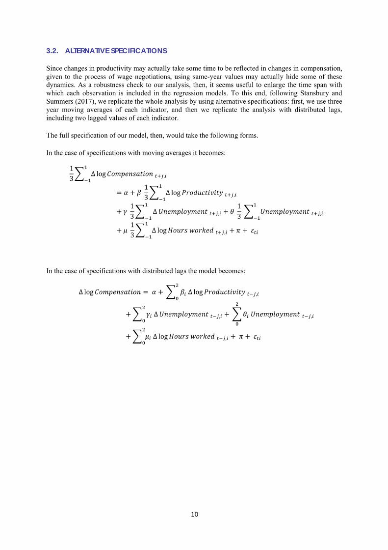
3.2. ALTERNATIVE SPECIFICATIONS

Since changes in productivity may actually take some time to be reflected in changes in compensation, given to the process of wage negotiations, using same-year values may actually hide some of these dynamics. As a robustness check to our analysis, then, it seems useful to enlarge the time span with which each observation is included in the regression models. To this end, following Stansbury and Summers (2017), we replicate the whole analysis by using alternative specifications: first, we use three year moving averages of each indicator, and then we replicate the analysis with distributed lags, including two lagged values of each indicator.

The full specification of our model, then, would take the following forms.

In the case of specifications with moving averages it becomes: 13 ∆ log ,= + 13 ∆ log ,+ 13 ∆ , + 13 ,+ 13 ∆ log , + +

In the case of specifications with distributed lags the model becomes:

∆ log = + ∆ log ,+ ∆ , + ,+ ∆ log , + +

10

4. RESULTS 4.1. FULL SAMPLE OF 34 COUNTRIES

e same. We also test our panel for panel-level heteroskedasticity and autocorrelation (See appendix).

ble 4.1. Changes in compensation and in productivity (full sample, full period, single years)

--

----

---

ro

(IV): F( 1, 33) = 38.13 Prob > F = 0.0000

cyclical conditions and structural characteristics of the labour market, this share nevertheless falls.

iated with the average number of hours worked per employed person is also negative and significant.

First of all, we take a look at the full sample of 34 advanced economies; we want to know whether a significant relation exists between productivity and compensation and whether it is positive or negative. Second, if this relation is positive and significant, we want to know how close it is to one: a positive, significant, and one-to-one relation would mean that productivity increases are fully transferred into compensations; conversely a relation significantly lower than one would imply the existence of a significant gap between productivity and compensation. We use data measured per hours, but we perform robustness tests with the same indicators measured per employed person, and the results are th

Ta ----------------------------------- ---------- --------- ----- ------- Compensation | (I) (II) (III) (IV) -------------+--------------------------------------------------Productivity | .678*** .670*** .624*** .521*** | (.074) (.072) (.071) (.078) Unemp change | -.328* -.200) -.290* | (.131) (.129 (.120) Unemp rate | -.298*** -.284*** | (.050) (.049) Hours per emp| -.622*** | (.111) _cons | .640*** .671*** 2.967** 2.887*** * | (.164) (.159) (.422) (.422) -------------+------------------------------------------------ N | 1229 1229 1228 1218 r2 | .194 .207 .266 .299 r2_a | .194 .206 .265 .296 ---------------------------------------------------------------

Note: bust standard errors; legend: * p<0.05; ** p<0.01; *** p<0.001 (I): F( 1, 33) = 19.09 Prob > F = 0.0001 (II): F( 1, 33) = 20.99 Prob > F = 0.0001 (III): F( 1, 33) = 27.95 Prob > F = 0.0000

The results of the first baseline regression for the whole panel suggest that there is a significant and positive association between real productivity and real compensation: as in Stansbury and Summers (2017), we find that between half and two thirds of productivity gains are transferred to workers income. As we include controls for

We test the robustness of these results to alternative specifications, by using moving averages and distributed lags. The robustness analysis confirms the validity of our initial results: in all specifications the coefficient associated with changes in productivity is positive, significantly different from zero, and also significantly different from one. The coefficient associated with changes in unemployment, although negative as one would have expected, is not always significant, it becomes so in the distributed lags specifications. The coefficient associated with the unemployment rate, instead, is strongly significant in all specifications in which it is included. The coefficient assoc

11

Graph 4.1. Changes in compensation and in productivity (full sample, full period, alternative specifications)

Note: The chart shows the estimated coefficients of various specifications of the model; the lines represent 95% confidence intervals.

Source: Commission services

These results imply that over the past half century, in the advanced economies, there has been a significant relation between productivity and compensation trends, the two have moved together, however a significant gap has been accumulated, so that not all gains from productivity are actually transferred to compensations. The fact that changes in unemployment only become significant with a lag, confirms the intuition that negative unemployment shocks put downward pressure on wages, but this takes some time to materialise. The rate of unemployment, instead, is always very significant and negatively influences compensations, meaning that when and where it is higher labour pay growth is lower; this confirms the idea that it is a good indicator of cyclical conditions, as argued by Bivens and Mishel (2017). The number of hours worked per employed person too has a strongly significant and negative coefficient, acting as an additional factor explaining downward pressure on compensation.

Differently from what previous studies on the US only had found, when we consider the full sample of advanced countries, we find that the coefficients associated with changes in productivity are significantly different, not only from zero, but also from one. This implies that the gap between productivity and compensation exists and is significant; in other words, we can say that over the past half century, in advanced economies, productivity gains did not translate fully to workers pay.

4.2. THE EU

We want to focus now on the EU; therefore we repeat the analysis only for the 28 member states. As a further step, we also include the euro area dummy; in the main specification we use the narrow euro area membership, but in the robustness tests we also use the broad peg to the euro or membership in the ERM.

12

Table 4.2. Changes in compensation and in productivity (EU 28, full period, single years) ------------------------------------------------------------------------------- Compensation | (I) (II) (III) (IV) (V) (VI) -------------+----------------------------------------------------------------- Productivity | .655*** .648*** .602*** .496*** .498*** .477*** | .072 .071 .080 .076 .085 .086 Unempl change| -.258* -.130 -.205* -.353** -.218* | .114 .108 .097 .104 .091 Unemp rate | -.298*** -.287*** -.282*** | .051 .051 .051 Hours per emp| -.650*** -.697*** -.658*** | .119 .139 .117 Euro Area | -.646* -.333 | .238 .294 _cons | .750*** .776*** 3.274*** 3.223*** 1.100*** 3.322*** | .167 .164 .455 .464 .239 .513 -------------+----------------------------------------------------------------- N | 985 985 984 974 975 974 r2 | .195 .204 .274 .313 .253 .314 r2_a | .194 .202 .272 .310 .250 .310 -------------------------------------------------------------------------------

Note: robust standard errors; legend: * p<0.05; ** p<0.01; *** p<0.001 (I): F( 1, 27) = 23.16 Prob > F = 0.0001 (II): F( 1, 27) = 24.65 Prob > F = 0.0000 (III): F( 1, 27) = 32.50 Prob > F = 0.0000 (IV): F( 1, 27) = 44.03 Prob > F = 0.0000 (V): F( 1, 27) = 36.93 Prob > F = 0.0000 (VI): F( 1, 27) = 35.00 Prob > F = 0.0000

The results for the EU are broadly similar to those of the full panel, the coefficients associated with productivity changes are strongly significant and positive, however we see that they are smaller than in the full sample with non-EU countries, in all specifications of the model. In the EU the extent to which productivity growth translates into compensation is between 50% and 60%, and is significantly different from one, confirming the productivity-pay gap. As in the full sample, we observe the strong significance of the rate of unemployment and of the number of hours worked per employed person, both negatively associated with rise in compensation, as one would expect.

Interestingly, the coefficient associated with membership in the monetary union is negative, but only significant when the rate of unemployment is not included in the model; when the overall rate of unemployment is factored in the equation, it "absorbs" the whole significance of the euro area dummy. The interpretation of this finding is that within the euro area, other things equal, the rate of unemployment has a more significant and negative effect on the average worker's compensation than outside. This is consistent with the notion that in a system of fixed exchange rates, the lack of external adjustment mechanism puts more emphasis on internal adjustment through the labour market, making wages more responsive to the unemployment rate, in the short term.

13

Graph 4.2. Changes in compensation and in productivity (EU 28, full period, alternative specifications)

Note: The chart shows the estimated coefficients of various specifications of the model; the lines represent 95% confidence intervals.

Source: Commission services

When we test the robustness of these results the picture does not change much compared with the baseline model with single year data, and the results confirm that the findings from our model are pretty robust to different methods and specifications. The coefficient associated with productivity changes is always positive, significantly different from zero, and also from one, which implies that about two thirds of increases in productivity are transferred to compensations, but the gap exists and is significant. As in the full sample, in the EU as well, changes in unemployment become significant with a lag. The euro area dummy, however, loses significance in the longer term, as showed by the alternative specifications with moving averages and distributed lags.

One of the major events in the process of EU integration was the creation of the monetary union, which comprised eleven countries at its inception, in 1999, but then grew to the current 19 member states. Its creation may have represented an important structural change in the region; therefore it seems reasonable to study the differences between the two periods, before and after 1999. We run the same model as for the full period.

When we study the period between 1970 and 1998, the coefficient associated with productivity changes is positive and significant in all specifications, as expected, and its value is higher than in the full period sample. As a matter of fact, it is not always significantly different from one, meaning that in the last decades of the past century increases in productivity substantially translated into pay rises for workers, the gap was not significant.

14

Graph 4.3. Changes in compensation and in productivity (EU 28, before and after EMU, single years)

Note: The chart shows the estimated coefficients of various specifications of the model; the lines represent 95% confidence intervals.

Source: Commission services

We then study the relation in the period after the introduction of the euro, and find that the extent to which productivity gains fed compensation somehow fell. On average, only half of those gains translated into pay rises, the gap becomes much more significant. To sum up, we cannot argue that the establishment of the EMU represented a clear-cut structural break in the productivity-pay relation, but we find evidence that in the EMU period this link somehow weakened. The aggregate analysis, however, may hide some heterogeneity at country level in the Euro Area, which will be the subject of another study, as well as the specific impact of other factors, which may be different from one country to another.

4.3. THE NON-EU

If we run a panel regression of the six non EU countries included in our dataset we find less significant, although similar results.

Table 4.3. Changes in compensation and productivity (panel, non EU countries, full period, single years) ------------------------------------------------------------------ Compensation | (I) (II) (III) (IV) -------------+---------------------------------------------------- Productivity | .838* .828* .785* .657* | (.265) (.228) (.248) (.238) Unempl change| -1.165 -1.036 -1.401 | (1.046) (1.128) (1.085) Unemp rate | -.282 -.192 | (.205) (.166) Hours per emp| -.735*** | (.092) _cons | .120 .186 1.600 1.134 | (.485) (.393) 1.359) (1.132) -------------+---------------------------------------------------- N | 244 244 244 244 r2 | .197 .266 .279 .306 r2_a | .195 .260 .267 .294 ------------------------------------------------------------------

Note: robust standard errors; legend: * p<0.05; ** p<0.01; *** p<0.001

15

Given the high heterogeneity of the group, coupled with the small number of countries, though, it seems more appropriate to replicate the analysis for each individual country.

As expected, the group of country is extremely heterogeneous and the results are quite different. The estimated coefficients associated with productivity are significant, signalling that the link between productivity and compensation is strong, in the US, Canada, Japan, and Iceland; they do not seem to be significant in the case of Switzerland and Norway, though. In Iceland, there seems to be a one-for-one relation between the two key variables, meaning that a one percentage rise in productivity generally translates into a one percentage rise in workers' pay. These coefficient are lower in the US, Canada and Japan. In the case of Japan it is very significantly different from one, signalling a significant gap between productivity and pay, and in Canada it is moderately different from one (at the 95% level, but not at 99%).

Graph 4.4. Changes in compensation and in productivity in individual countries (non EU countries, full period, single years)

Note: The chart shows the estimated coefficients of various specifications of the model; the lines represent 95% confidence intervals.

Source: Commission services

In the case of the US the coefficient is not significantly different from one, which confirms the finding of other studies which specifically analysed the US case, at least when average compensation is the concept analysed. Interestingly, this applies also to the full specification where all controls are included, supporting the "linkage" view the authors present. However, it is also important to remind that this analysis is done on "average" and not on "median" compensation, so that the overall gap between the typical worker's pay and productivity is underestimated, as explained in the introduction.

Another interesting observation is that the gap is particularly significant in Switzerland and Norway, and to a lower extent in Japan. The rate of unemployment is a significant factor associated with lower compensation in Canada and Japan, while its variation significantly and negatively relates to pay in Norway and Iceland2.

2 In Iceland the estimated coefficient is -4.511, with a 95% confidence interval between -5.957 and -3.066, too low to be shown in the chart.

16

5. IMPLICATIONS

Once observed the co-movement of real compensation and productivity over time, and established that a significant gap between the two exists, we now want to understand whether this gap has any implications on other macroeconomic variables. The existence of such a gap also reflects the observed trends of labour incom re sha e. We first construct an indicator measuring the ga

mpensations: = ∆ log − ∆ log

p between increases in productivity and in co

been recently labelled as "secular stagnation" as "the defining issue of our age" (Summers, 2013).

ould be significantly and positively associated with the gap between productivity and compensation.

To test this hypothesis we run the foll

yment rate and changes in unemployment, we also add the inflation rate, and a euro area dummy.

ount balance on GDP, therefore with a reduction in domestic demand, thus supporting our hypothesis.

The fact that for a long period real pay remains subdued compared to real productivity matters not just for ethical reasons or political preferences, but also because it may help shed some light about broad macroeconomic trends. A prolonged gap between the growth rate of compensation and of productivity may be associated with a tendency to subdued aggregate demand over time, a phenomenon whose consequences have

If the gap between productivity and pay is relevant, we should probably see within each country an association between it and the level of domestic demand compared with total output. Within each country, this second gap, the one between domestic demand and total output, is the mirror image of its current account balance, therefore this sh

owing regression: ∆ = + + ∆ + + + + We first test the relevance of the GAP alone, and progressively add controls for cyclical conditions, in the form of unemplo

The gap between productivity and compensation seems indeed positively associated with the current account balance, that we use as a proxy for subdued domestic demand. A one percentage point increase in the gap is associated with a 0.1 increase in the current acc

17

Table 5.1. Current account balance and gap between compensation and productivity (full sample, full period, single years) ---------------------------------------------------------------------

Dependent: Current Account balance on GDP | (I) (II) (III) (IV) -------------+------------------------------------------------------- Gap | .150*** .114** .100** .101** | 0.037 0.039 0.033 0.033 Unemp rate | .047 .054* .048 | 0.025 0.023 0.024 Unemp change | .596*** .586*** .596*** | 0.102 0.102 0.103 Inflation | .006*** .006*** | 0.001 0.001 Euro Area | .358* | 0.132 _cons | .054*** -.302 -.387* -.433* | 0.006 0.183 0.167 0.159 -------------+------------------------------------------------------- N | 1219 1215 1214 1214 r2 | .03950754 .14626647 .15120991 .15380824 r2_a | .03871831 .14415153 .14840167 .15030579 ---------------------------------------------------------------------

Note: Robust standard errors; legend: * p<0.05; ** p<0.01; *** p<0.001

Further work is needed on this point to disentangle the extent to which a gap between productivity and compensation has a negative and significant impact on domestic demand, but this result provides a first hint.

6. CONCLUSIONS

We have tested the hypothesis that over the past half century in a set of 34 advanced economies productivity growth substantially translated into increases in workers' compensation. We have found that the two dynamics are indeed linked, but there is no one-to-one relation so to say that all productivity gains fed workers' pay: there is indeed a significant gap between the two. Importantly, our results underestimate the size of this gap for two reasons: first, our data refer to "average" and not "median" compensation, so given the increasingly unequal distribution of wages, the gap between average productivity growth and the compensation of the "typical worker" is probably larger than what we find; second, we use data for total compensation, because we could not single out production/non-supervisory workers' pay, which tend to be lower, as analyses of the specific case of the US prove. Cyclical conditions as well as labour market structures too greatly affect this relation. Over the past half century in advanced economies, an increase of one percentage point in the rate of productivity growth has been associated with an increase in the rate of average compensation growth of 0.6 to 0.8 percentage points. A specific look at the EU suggests these results also apply to Europe.

here it is higher. The country-specific analysis of EU countries will be the subject of another work.

An important aspect of these findings is that the aggregate panel approach may actually mask some heterogeneity between countries: the country-specific analysis of non-EU countries, in fact, shows important differences between countries where the coefficient associated with productivity was not significantly different from one, and countries where it was not significantly different from zero. A plausible hypothesis is that policies for redistribution matter to explain the cross-country differences and to compensate the gap between productivity and pay w

The implications of these findings are manifold. First, productivity growth is a necessary but not sufficient condition for rising wages; as a consequence, policies aiming at rising productivity are certainly useful but clearly not sufficient to raise compensations of those who contribute to

18

productivity growth, as some have recently argued (Bernstein, 2015). Second, the deceleration in compensation growth does not only reflect slower productivity growth, but other factors, such as structural conditions in the labour market, concur in determining it. Third, high levels of unemployment greatly affect the extent to which workers are able to reap the benefits of fast productivity growth, due to their reduced bargaining power. Fourth, although this topic has recently gained prominence in the US, our analysis shows that these findings apply to the EU and to other advanced economies as well. The implications, therefore, are not just relevant for the US, but for all advanced economies. Fifth, to the extent that the gap between productivity and pay affects aggregate demand, and may therefore have an influene on inflation and interest rates, understanding its determinants is crucial for the conduct of macroeconomic policies.

r than productivity growth can have positive effect on the latter, in a kind of inverse hysteresis effect.

In order to increase living standards and reduce inequality, pro-growth policies aiming at boosting productivity are not sufficient. They should be complemented by policies to pursue full employment3, if the link between productivity and pay is to be fully restored, and by policies for redistribution, in those cases where the gap between productivity and pay is larger. The logic question that follows, which is also an important avenue for future research, is to what extent policies to pursue full employment can close the observed gap between compensation and productivity, and to what extent prolonged periods of full employment and compensation growth equal to or highe

3 Jared Bernstein (2017) suggests several measures in this directions ("pushing for higher minimum wages, full employment (direct job creation), progressive taxation, collective bargaining, overtime rules, gender equity, a robust safety net, more balanced trade, financial market regulation, and so on are gap-closing ideas that we know will help") and importantly points out that they are not in antithesis with pro-growth policies.

19

REFERENCES

Bernstein, Jared (2015) What’s (not) up with productivity growth, part 1: Why this key variable is slowing across advanced economies. Washington Post, July 28, 2015. Accessible at: https://www.washingtonpost.com/posteverything/wp/2015/07/28/whats-not-up-with-productivity-growth-part-1-why-this-key-variable-is-slowing-across-advanced-economies/?utm_term=.6a8cf6c45fa6

Bernstein, Jared (2017) Wages, productivity, progressive policies, and serial correlation: I weigh in on an important, interesting debate. November 20th, 2017. Accessible at: http://jaredbernsteinblog.com/wages-productivity-progressive-policies-and-serial-correlation-i-weigh-in-on-an-important-interesting-debate/

Bivens J. and L. Mishel (2015) “Understanding the Historic Divergence between Productivity and a Typical Worker's Pay: Why It Matters and Why It's Real". Economic Policy Institute.

Bivens J. and L. Mishel (2017) New paper on pay-productivity link does not overturn EPI findings. Posted November 9, 2017 http://www.epi.org/blog/new-paper-on-pay-productivity-link-does-not-overturn-epi-findings/

Council of Economic Advisers (2014) The Economic Report of the President together with the Annual Report of the Council of Economic Advisers. Washington, DC.

Draghi, Mario (2017) Introductory statement to the press conference, President of the ECB, Frankfurt am Main, 9 March 2017 https://www.ecb.europa.eu/press/pressconf/2017/html/is170309.en.html

Feldstein, M. (2008). “Did wages reflect growth in productivity?" Journal of Policy Modeling 30(4): 591-594.

Fleck, S., Glaser, J., & Sprague, S. (2011). The compensation-productivity gap: a visual essay. Monthly Labor Review, 134(1), 57-69.

Freeman, Richard B., and Lawrence F. Katz, eds. (1995). Differences and Changes in Wage Structures. Chicago, IL: University of Chicago Press.

IMF (2017) “Understanding the Downward Trend in Labor Income Shares”. World Economic Outlook, April, Ch.3 (121-172).

Lawrence, R.Z. (2016). “Does Productivity Still Determine Worker Compensation? Domestic and International Evidence”. Ch.2 in The US Labor Market: Questions and Challenges for Public Policy. American Enterprise Institute Press.

Marx, Karl, (1867–1883), Capital. Critique of Political Economy. (1 ed.). Hamburg: Verlag von Otto Meissner. Available online at: https://www.marxists.org/archive/marx/works/1867-c1/index.htm

Mishel, L., & Bernstein, J. (1994). The state of working America 1994-95 (Vol. 4). ME Sharpe.

Ricardo, 1911 [1817], p. 1 in 1911 edition) (Ricardo opening paragraph of his book On The Principles of Political Economy and Taxation (1817))

Smith, Adam, (1776), The Wealth of Nations, Book 1, Chapter 8 “Of the Wages of Labour“.

20

Stansbury, A. M., & Summers, L. H. (2017). Productivity and Pay: Is the link broken? (No. w24165). National Bureau of Economic Research.

Summers L. (2013), "IMF Economic Forum: Policy Responses to Crises", speech delivered at the IMF Annual Research Conference, November 8th.

Yellen, Janet. “Semiannual Monetary Policy Report to the Congress.” February 24, 2015; http://www.federalreserve.gov/newsevents/testimony/yellen20150224a.htm.

21

ANNEX I

Unit-root tests Im-Pesaran-Shin unit-root test for real hourly compensation (d.log) ------------------------------------------------------------------------------ Ho: All panels contain unit roots Number of panels = 34 Ha: Some panels are stationary Avg. number of periods = 36.15 AR parameter: Panel-specific Asymptotics: T,N -> Infinity Panel means: Included sequentially Time trend: Not included ADF regressions: No lags included ------------------------------------------------------------------------------ Fixed-N exact critical values Statistic p-value 1% 5% 10% ------------------------------------------------------------------------------ t-bar -4.1067 (Not available) t-tilde-bar -3.2959 Z-t-tilde-bar -13.6350 0.0000 ------------------------------------------------------------------------------ Im-Pesaran-Shin unit-root test for real hourly productivity (d.log) ------------------------------------------------------------------------------ Ho: All panels contain unit roots Number of panels = 34 Ha: Some panels are stationary Avg. number of periods = 37.18 AR parameter: Panel-specific Asymptotics: T,N -> Infinity Panel means: Included sequentially Time trend: Not included ADF regressions: No lags included ------------------------------------------------------------------------------ Fixed-N exact critical values Statistic p-value 1% 5% 10% ------------------------------------------------------------------------------ t-bar -4.4109 (Not available) t-tilde-bar -3.4607 Z-t-tilde-bar -14.8039 0.0000 ------------------------------------------------------------------------------

22

ANNEX II

Test for panel-level heteroskedasticity and autocorrelation Iteration 1: tolerance = .02297993 Iteration 2: tolerance = .00524203 Iteration 3: tolerance = .00117911 Iteration 4: tolerance = .00026408 Iteration 5: tolerance = .00005932 Iteration 6: tolerance = .00001456 Iteration 7: tolerance = 4.411e-06 Iteration 8: tolerance = 1.280e-06 Iteration 9: tolerance = 3.614e-07 Iteration 10: tolerance = 1.000e-07 Iteration 11: tolerance = 2.729e-08 Cross-sectional time-series FGLS regression Coefficients: generalised least squares Panels: heteroskedastic Correlation: no autocorrelation Estimated covariances = 34 Number of obs = 1,218 Estimated autocorrelations = 0 Number of groups = 34 Estimated coefficients = 5 Obs per group: min = 16 avg = 35.82353 max = 58 Wald chi2(4) = 922.14 Log likelihood = -2686.942 Prob > chi2 = 0.0000 ------------------------------------------------------------------------------ comphr_dl | Coef. Std. Err. z P>|z| [95% Conf. Interval] -------------+---------------------------------------------------------------- prodhr1_dl | .4801926 .0273934 17.53 0.000 .4265025 .5338826 U | -.136444 .0149816 -9.11 0.000 -.1658073 -.1070807 u_d | -.112379 .0538837 -2.09 0.037 -.2179891 -.0067688 hxemp_dl | -.7446934 .0559884 -13.30 0.000 -.8544286 -.6349582 _cons | 1.509446 .1269286 11.89 0.000 1.260671 1.758222 ------------------------------------------------------------------------------ Iteration 1: tolerance = 0 Cross-sectional time-series FGLS regression Coefficients: generalised least squares Panels: homoskedastic Correlation: no autocorrelation Estimated covariances = 1 Number of obs = 1,218 Estimated autocorrelations = 0 Number of groups = 34 Estimated coefficients = 5 Obs per group: min = 16 avg = 35.82353 max = 58 Wald chi2(4) = 501.04 Log likelihood = -3124.557 Prob > chi2 = 0.0000 ------------------------------------------------------------------------------ comphr_dl | Coef. Std. Err. z P>|z| [95% Conf. Interval] -------------+---------------------------------------------------------------- prodhr1_dl | .6346498 .0384709 16.50 0.000 .5592483 .7100514 U | -.1232454 .0213716 -5.77 0.000 -.165133 -.0813578

23

u_d | -.3656937 .0741603 -4.93 0.000 -.5110452 -.2203422 hxemp_dl | -.514702 .0826822 -6.23 0.000 -.6767561 -.3526479 _cons | 1.483935 .1987706 7.47 0.000 1.094352 1.873518 ------------------------------------------------------------------------------ . local df = e(N_g) - 1 . lrtest hetero . , df(`df') Likelihood-ratio test LR chi2(33) = 875.23 (Assumption: . nested in hetero) Prob > chi2 = 0.0000

24

ANNEX III

Detailed results of the alternative specifications

In the alternative specifications, the results are not significantly different, although the associated coefficients are slightly higher:

Table a: Full sample, full period (moving averages) ------------------------------------------------------------------------------ Variable | bas ud udu uduh -------------+---------------------------------------------------------------- ma3prodh | .76621605*** .76044283*** .67010043*** .61836832*** ma3du | -.34907996* -.24018379 -.28266037* ma3u | -.26466169*** -.25966932*** ma3hxemp | -.34712161* _cons | .42281896* .45469591* 2.6204115*** 2.5781219*** -------------+---------------------------------------------------------------- N | 1161 1161 1160 1150 r2 | .28917771 .30960546 .40933315 .41835376 r2_a | .2885644 .30841307 .40780027 .41632181 ------------------------------------------------------------------------------ legend: * p<0.05; ** p<0.01; *** p<0.001 F( 1, 33) = 9.19 Prob > F = 0.0047 F( 1, 33) = 9.51 Prob > F = 0.0041 F( 1, 33) = 19.79 Prob > F = 0.0001 F( 1, 33) = 18.72 Prob > F = 0.0001

Table b: Full sample, full period (distributed lags) ------------------------------------------------------------------------------ Variable | baselag lagsud lagsudu lagsuduh -------------+---------------------------------------------------------------- prodhr1_dl | .52235973*** .56416663*** .54594434*** .43273944*** l1prod | .10328136* .11775** .08272761* .10227828** l2prod | .15190342** .11263077* .08973991* .1104483* u_d | -.14968662 -.13305542 -.24762222 l1du | -.26367584* -.17334521 -.08873236 l2du | -.43466631*** -.29882792** -.30194119** U | -.17574154*** -.17236094*** hxemp_dl | -.60899658*** l1hemp | .01609274 l2hemp | .14429936* _cons | .35131624* .38050529* 1.8473946*** 1.8329041*** -------------+---------------------------------------------------------------- N | 1167 1167 1165 1154 r2 | .17655019 .24210629 .25981643 .30272561 r2_a | .17442607 .23818615 .25533822 .29662522 ------------------------------------------------------------------------------ legend: * p<0.05; ** p<0.01; *** p<0.001 test ( prodhr1_dl+ l1prod+ l2prod) = 1 ( 1) prodhr1_dl + l1prod + l2prod = 1 F( 1, 33) = 7.94 Prob > F = 0.0081 ** F( 1, 33) = 7.53 Prob > F = 0.0097 ** F( 1, 33) = 13.94 Prob > F = 0.0007 *** F( 1, 33) = 18.64 Prob > F = 0.0001 ***

Note: lagged values for the unemployment rate omitted because of collinearity.

25

Table c: The EU, full period (moving averages) ------------------------------------------------------------------------------ Variable | eu euud euudu euuduh -------------+---------------------------------------------------------------- ma3prodh | .7581929*** .7524374*** .66003977*** .60527739*** ma3du | -.28978925* -.18194658 -.21830327 ma3u | -.26476444*** -.26081132*** ma3hxemp | -.39144756* _cons | .49342595** .52358543** 2.8789032*** 2.8451566*** -------------+---------------------------------------------------------------- N | 929 929 928 918 r2 | .29953827 .31580997 .43339001 .44571271 r2_a | .29878265 .31433224 .43155037 .44328429 ------------------------------------------------------------------------------ F( 1, 27) = 10.85 Prob > F = 0.0028 F( 1, 27) = 10.91 Prob > F = 0.0027 F( 1, 27) = 23.92 Prob > F = 0.0000 F( 1, 27) = 23.57 Prob > F = 0.0000 ---------------------------------------------- Variable | nou ea -------------+-------------------------------- ma3prodh | .65407463*** .59574179*** ma3du | -.34636614** -.22267274 ma3hxemp | -.47153647* -.39688771* EA | -.29358585 -.08717265 ma3u | -.25980004*** _cons | .69030654* 2.8838671*** -------------+-------------------------------- N | 919 918 r2 | .33489317 .44589718 r2_a | .33198242 .44285934

legend: * p<0.05; ** p<0.01; *** p<0.001 F( 1, 27) = 10.37 Prob > F = 0.0033 F( 1, 27) = 14.29 Prob > F = 0.0008

Table d: The EU, full period (distributed lags) ------------------------------------------------------------------------------ Variable | eulag eulagsud eulagsudu eulagsuduh -------------+---------------------------------------------------------------- prodhr1_dl | .5008735*** .5454665*** .52729215*** .4045861*** l1prod | .08577046 .10720505* .07136895 .10474185** l2prod | .19410364*** .15257006*** .12989275** .15316611** u_d | -.07888095 -.06688975 -.1699859 l1du | -.25576276* -.16933761 -.07699186 l2du | -.45534123*** -.31985373** -.33902077** U | -.17002098*** -.1657268*** l1u | (omitted) (omitted) l2u | (omitted) (omitted) hxemp_dl | -.65577179*** l1hemp | .03144346 l2hemp | .16723011* _cons | .39584857* .40963274* 1.957474*** 1.9272625*** -------------+---------------------------------------------------------------- N | 931 931 929 918 r2 | .19037175 .26503775 .28533004 .34092816 r2_a | .1877516 .26026527 .27989823 .33366166 ------------------------------------------------------------------------------ legend: * p<0.05; ** p<0.01; *** p<0.001

26

--------------------------------------------- Variable | eanou eafull -------------+-------------------------------- prodhr1_dl | .41196306*** .39882245*** l1prod | .13217643** .09972801* l2prod | .16012251*** .14757363** u_d | -.19417941 -.17974114 l1du | -.16599002 -.07939714 l2du | -.47956931*** -.34158044** hxemp_dl | -.65966212*** -.65542168*** l1hemp | .03168797 .02761528 l2hemp | .14322872* .15902247* EA | -.62348148 -.55289282 l1ea | .67046673 .6519498 l2ea | -.30905223 -.24532446 U | -.16381782*** l1u | (omitted) l2u | (omitted) _cons | .57466825 1.9969565** -------------+-------------------------------- N | 919 918 r2 | .32283148 .3416886 r2_a | .31386236 .33222173 ---------------------------------------------- legend: * p<0.05; ** p<0.01; *** p<0.001

Table e: Non EU 6 – by country (single years) ------------------------------------------------------------------------------ Variable | us ca ja ch -------------+---------------------------------------------------------------- prodhr1_dl | .73959537*** .66724021*** .447285*** .11262128 u_d | -.03249265 .376517 -.15890006 -.12521509 U | -.200396 -.54627676*** -.39917126* -.18242086 hxemp_dl | -.23705708 -.38444168 -.6126455*** -1.4061598*** _cons | 1.3619284* 4.7577233*** 1.3064562 1.3831998 -------------+---------------------------------------------------------------- N | 48 46 35 24 r2 | .55259664 .59243203 .73408476 .76324181 r2_a | .51097772 .5526693 .6986294 .71339798 ------------------------------------------------------------------------------ legend: * p<0.05; ** p<0.01; *** p<0.001 F( 1, 43) = 2.63 USA Prob > F = 0.1124 F( 1, 41) = 6.80 CAN Prob > F = 0.0127 F( 1, 30) = 24.82 JAP Prob > F = 0.0000 F( 1, 19) = 33.70 CHE Prob > F = 0.0000 ---------------------------------------------- Variable | nor ice -------------+-------------------------------- prodhr1_dl | .15787444 .96219337* u_d | -1.2540427*** -4.5113914*** U | -.45967447 .22487085 hxemp_dl | -.48453163 -.45389095 _cons | 3.379835** -.70033418 -------------+-------------------------------- N | 46 45 r2 | .35912135 .52316353 r2_a | .2965966 .47547988 ---------------------------------------------- legend: * p<0.05; ** p<0.01; *** p<0.001 F( 1, 41) = 26.14 NOR Prob > F = 0.0000 F( 1, 40) = 0.01 ICE Prob > F = 0.9213

27

Table f: Non EU 6 – by country (moving averages) ------------------------------------------------------------------------------ Variable | us ca ja ch -------------+---------------------------------------------------------------- ma3prodh | .83604953*** .59972012** .56300638*** -.29495927 ma3du | -.13890712 -.21926407 -.50587646 -.45639921 ma3u | -.2093417*** -.39205891*** -.31808663* -.31162951 ma3hxemp | -.14107975 -1.0085429* -.72738198*** -1.5738325*** _cons | 1.2886918** 3.3857146*** .71522369 2.306959** -------------+---------------------------------------------------------------- N | 46 44 33 22 r2 | .73426756 .66210165 .87212222 .88256172 r2_a | .70834244 .62744541 .85385396 .85492919 ------------------------------------------------------------------------------ legend: * p<0.05; ** p<0.01; *** p<0.001 F( 1, 41) = 1.87 USA Prob > F = 0.1792 F( 1, 39) = 5.22 CAN Prob > F = 0.0278 F( 1, 28) = 39.04 JAP Prob > F = 0.0000 F( 1, 17) = 81.95 CHE Prob > F = 0.0000 ---------------------------------------------- Variable | nor ice -------------+-------------------------------- ma3prodh | -.00540109 1.6806432*** ma3du | -1.650673*** -3.2087393*** ma3u | -.19282256 .25126284 ma3hxemp | -.83087007 1.7794051* _cons | 2.6726981* -1.3534805 -------------+-------------------------------- N | 44 43 r2 | .35371672 .69766231 r2_a | .28743125 .66583729 ---------------------------------------------- legend: * p<0.05; ** p<0.01; *** p<0.001 F( 1, 39) = 27.69 NOR Prob > F = 0.0000 F( 1, 38) = 4.85 ICE Prob > F = 0.0338

Table g: Non EU 6 – by country (distributed lags) ------------------------------------------------------------------------------ Variable | usa can jap che -------------+---------------------------------------------------------------- prodhr1_dl | .89505883*** .76310575*** .41844746* -.06271641 l1prod | .19633829 -.12720926 .1826781 -.31131459 l2prod | -.13271203 -.35528793* -.0448782 .15345241 u_d | .45262318 (omitted) (omitted) (omitted) l1du | (omitted) (omitted) (omitted) (omitted) l2du | .04231086 -.12076832 -.05905801 -.09075511 U | -.47685776* -.07083134 -.55825824 -1.107539 l1u | (omitted) -.90434606* .30300828 1.7619215 l2u | .41604646 .564424 -.03177101 -1.0713082 hxemp_dl | -.18886479 -.34909073 -.61892042** -1.8274695*** l1hemp | -.11581008 -.06495629 -.13108347 -.02921436 l2hemp | .19172549 -.09598449 -.10086999 .114986 _cons | .15715715 4.1107765** .52793073 2.4725931 -------------+---------------------------------------------------------------- N | 46 44 35 24 r2 | .5983591 .68225511 .77373229 .82074911 r2_a | .48360456 .58596877 .67945408 .68286381 ------------------------------------------------------------------------------

28

29

-------------+-------------------------------- Variable | nor ice -------------+-------------------------------- prodhr1_dl | .25593773 1.120496* l1prod | -.08227098 .50559445 l2prod | .01894587 .15043888 u_d | (omitted) (omitted) l1du | .30455511 (omitted) l2du | .06269354 .48532038 U | -1.3697943* -3.8100242*** l1u | (omitted) 4.5139566* l2u | 1.0202757 -.35542913 hxemp_dl | -.53904709 .3212579 l1hemp | .17682386 .10477833 l2hemp | .45775411 .90562819 _cons | 3.1867272* -2.0036725 -------------+-------------------------------- N | 44 43 r2 | .40904023 .52499924 r2_a | .22996151 .3765615 ---------------------------------------------- legend: * p<0.05; ** p<0.01; *** p<0.001 F( 1, 35) = 0.03 USA Prob > F = 0.8635 F( 1, 33) = 7.81 CAN Prob > F = 0.0086 ** F( 1, 24) = 5.43 JAP Prob > F = 0.0286 * F( 1, 13) = 12.71 CHE Prob > F = 0.0035 ** F( 1, 33) = 6.72 NOR Prob > F = 0.0141 * F( 1, 32) = 0.93 ICE Prob > F = 0.3418

EUROPEAN ECONOMY DISCUSSION PAPERS European Economy Discussion Papers can be accessed and downloaded free of charge from the following address: https://ec.europa.eu/info/publications/economic-and-financial-affairs-publications_en?field_eurovoc_taxonomy_target_id_selective=All&field_core_nal_countries_tid_selective=All&field_core_date_published_value[value][year]=All&field_core_tags_tid_i18n=22617. Titles published before July 2015 under the Economic Papers series can be accessed and downloaded free of charge from: http://ec.europa.eu/economy_finance/publications/economic_paper/index_en.htm.

GETTING IN TOUCH WITH THE EU In person All over the European Union there are hundreds of Europe Direct Information Centres. You can find the address of the centre nearest you at: http://europa.eu/contact. On the phone or by e-mail Europe Direct is a service that answers your questions about the European Union. You can contact this service:

• by freephone: 00 800 6 7 8 9 10 11 (certain operators may charge for these calls),

• at the following standard number: +32 22999696 or • by electronic mail via: http://europa.eu/contact.

FINDING INFORMATION ABOUT THE EU Online Information about the European Union in all the official languages of the EU is available on the Europa website at: http://europa.eu. EU Publications You can download or order free and priced EU publications from EU Bookshop at: http://publications.europa.eu/bookshop. Multiple copies of free publications may be obtained by contacting Europe Direct or your local information centre (see http://europa.eu/contact). EU law and related documents For access to legal information from the EU, including all EU law since 1951 in all the official language versions, go to EUR-Lex at: http://eur-lex.europa.eu. Open data from the EU The EU Open Data Portal (http://data.europa.eu/euodp/en/data) provides access to datasets from the EU. Data can be downloaded and reused for free, both for commercial and non-commercial purposes.