The relationship between abnormal

inventory growth and future earnings for

U.S. public retailers

Saravanan Kesavan1, Vidya Mani2

Kenan-Flagler Business School, University of North Carolina at Chapel Hill, Chapel Hill, NC 27599.

Email: 1skesavan@unc.edu, 2vidya_mani@unc.edu

In this paper we examine the relationship between inventory levels and one-year ahead earnings of

retailers using publicly available financial data. We use benchmarking metrics obtained from operations

management literature to demonstrate an inverted-U relationship between abnormal inventory growth and

one-year ahead earnings per share for retailers. We also find that equity analysts do not fully incorporate

the information contained in abnormal inventory growth of retailers in their earnings forecasts resulting in

systematic biases. Finally, we show that an investment strategy based on abnormal inventory growth

yields abnormal returns of 11.8% (p<0.001).

 

2  

1. Introduction

Retailers pay close attention to inventory growth in their stores as it can have a significant impact on their

future financial performance. Too much of inventory in their stores could result in future markdowns

while too little inventory could result in lower demand in the future due to customer dissatisfaction with

poor service levels. Numerous anecdotes of poor inventory management leading to decline in financial

performance of retailers can be found in the business press. However, there is little empirical evidence on

the relationship between current inventory levels and future financial performance of retailers.

In fact, there is growing evidence that even Wall Street investors may have trouble understanding

the relationship between inventory levels and future financial performance of retailers. Kesavan et al.

(2010) find that even though inventory contains useful information to predict sales for retailers, Wall

street analysts fail to incorporate this information in their sales forecasts. Hendricks and Singhal (2009),

who examine excess inventory announcements of firms from multiple industry sectors including retail,

find that these announcements are associated with negative stock market reactions in a vast majority of

those cases. Since excess inventory would get reported only when such inventory problems become large

enough, their results suggest that the stock market investors failed to anticipate these announcements even

though they had access to past inventory levels of those firms.

In this paper, we are interested in examining the relationship between inventory and one-year

ahead earnings per share. We choose earnings per share because of the following reasons. First, earnings

per share is an important financial metric for firms and their forecasts form a key input to investment

decisions. Givoly and Lakonishok (1984) find that “earnings per share emerges from various studies as

the single most important accounting variable in the eyes of investors and the one that possesses the

greatest information content of any array of accounting variables.” Second, current evidence on the

relationship between inventory and one-year ahead earnings1 for retailers is weak. Accounting literature

that examined this question has yielded a mixed response. Abarbanell and Bushee (1997) do not find

evidence of this relationship for retailers but Bernard and Noel (1991) do. Even Bernard and Noel (1991),

who find inventory predicts earnings for retailers, assume a linear relationship between inventory and

earnings and find evidence for the same. Since earnings are a measure of profitability of the firm, one

might expect the relationship to be an inverted-U based on the operations management literature. This

raises the additional question of whether the inverted-U relationship which forms the building block of

inventory models at the SKU-level can be lost at the firm-level?

                                                            1 We use earnings and earnings per share interchangeably

3  

There are several challenges in testing the relationship between inventory and earnings at the

firm-level. First, raw inventory levels cannot be used to determine the relationship since it is correlated

with number of stores, sales etc. For example, inventory for a retailer could have grown either due to

presence of stale inventory or as a result of opening new stores. While the former would be associated

with lower earnings in the future, the latter would not. So, an appropriate method for normalizing

inventory is required before we test the relationship between inventory and earnings. Second, service

level information of retailers is not publicly available. So, it is difficult to figure out whether a retailer’s

inventory level is high because it is carrying excess inventory or if it is providing a high service level (Lai

2006). The former would be a negative signal of future earnings but the latter would not.

In this paper, we normalize inventory levels using the expectation model from Kesavan et al.

(2010) to obtain the expected inventory growth. Then we calculate abnormal inventory growth as the

deviation of actual inventory growth from expected inventory growth and use it as the benchmarking

metric to investigate the relationship between inventory and one-year ahead earnings. We investigate the

economic significance of the information content in abnormal inventory growth by examining if equity

analysts’ earnings forecasts incorporate information contained in abnormal inventory growth and test if an

investment strategy based on abnormal inventory growth would yield significant abnormal returns.

We use quarterly and annual financial data along with comparable store sales, total number of stores

and earnings per share for a large cross-section of U.S. retailers listed on NYSE, AMEX, or NASDAQ

from Standard & Poor’s Compustat database for our analysis. Equity analysts’ earnings forecasts are

collected from Institutional Brokers Estimates System (I/B/E/S). Stock returns inclusive of dividends are

obtained from CRSP. These are supplemented with hand-collected data from financial statements. Our

study period is fiscal years 1993-2009.

Our paper has the following findings. First, we demonstrate an inverted-U relationship between

abnormal inventory growth and one-year ahead earnings. Our results are robust to the metric used to

measure abnormal inventory growth. Second, we find that equity analysts do not fully incorporate the

information contained in past inventory resulting in systematic bias in their earnings forecasts; this bias is

predicted by previous year’s abnormal inventory growth. Third, we find that an investment strategy based

on abnormal inventory growth yields significant abnormal returns.

Our paper is closest to Kesavan et al. (2010) who study if inventory can be used to predict future sales

in the retail industry. They find that incorporating inventory and margin information significantly

improves sales forecasts. Further they find that analysts do not fully incorporate this information resulting

in predictable biases in their sales forecasts. We add to their findings by showing that inventory also

contains information useful to predict earnings in the retail industry. Since earnings are a function of sales

and expenses, we run several tests to show that inventory predicts earnings not only because it predicts

4  

sales but also because it predicts expenses for a retailer. Similarly we show that bias in analysts’ earnings

forecasts arises not only because analysts ignore information in inventory useful to predict sales, as shown

by Kesavan et al. (2010), but also because they fail to consider the impact of inventory on the expenses

for retailers. Finally, we analyze stock market data for retailers, not considered in Kesavan et al. (2010).

Our paper contributes to the operations management literature in the following ways. There is a

growing interest among researchers in operations management to examine firm-level inventory (Gaur et

al. 2005; Rumyantsev and Netessine 2007; Chen et al. 2005; Rajagopalan 2010). Many of these papers

are motivated to develop new benchmarking metrics that are useful to gauge the inventory performance at

the firm-level. Our paper complements this line of research by demonstrating that such benchmarking

metrics possess information useful to predict earnings and serve as a basis for investment strategies. In

addition, the research on firm-level inventory has sought to examine if the insights from the analytical

models also hold at the firm-level. Rumyantsev and Netessine (2007), for example, argue that this is

important to perform such tests to demonstrate to the high-level managers who deal with firm-level

inventory that they may benefit from understanding classical inventory models. Ours is the first paper to

demonstrate that the inverted-U relationship between inventory and profits, that forms the fundamental

building block of SKU-level literature, holds at the firm-level as well.

The paper is organized as follows. In §2 we discuss the operations management literature and

accounting literature that relates to our work. In §3 we discuss existing theory in operations management

to argue why changes in inventory levels could be considered as a signal of future earnings, §4 outlines

our research setup and §5 describes the methodology we adopt to calculate abnormal inventory growth. In

§6, we report results showing the relationship between abnormal inventory growth and one-year ahead

earnings while §7 investigates the economic significance of ignoring information contained in abnormal

inventory growth. Finally, we conclude with limitations and directions for future research in §8.

2. Literature Review

There has been significant interest in developing benchmarking metrics for firm-level inventory

performance. Gaur, Fisher and Raman (2005) study inventory turns and develop a metric, adjusted

inventory turns, to compare inventory productivity across firms. Rumyantsev and Netessine (2007) show

that increase in demand uncertainty, lead times, and margins, and decrease in economies of scale are

associated with increase in inventory levels. Chen et al. (2007) benchmark inventory performance using a

metric called abnormal days-of-inventory or AbI, which is defined relative to the segment’s average days-

of-inventory. Rajagopalan (2010) combines primary and secondary data to show that product variety,

along with other factors such as gross margin and economies of scale, affects the firm-level inventory

5  

carried by retailers. Our work adds to this literature by testing the efficacy of two of those metrics for

prediction purposes.

There is some evidence linking inventory performance to stock market performance of firms. Chen et

al. (2005) and Chen et al. (2007) find correlation between inventory changes and abnormal stock market

returns. Hendricks and Singhal (2005) show that announcement of supply chain glitches, which

commonly cause inventory problems, are associated with a negative stock market reaction. However,

these papers perform ex post facto analysis and hence do not test the informational content in inventory

levels for prediction purposes. Our paper adds to this literature by showing that inventory-based

benchmarking metrics may serve as basis for investments in the stock market.

Next, we would like to briefly review the accounting literature that relates to our work. Accounting

literature has shown some mixed evidence of the predictive power of inventory over earnings in the retail

sector. Bernard and Noel (1991) find that inventory predicts earnings in the retail industry but Abarbanell

and Bushee (1997) do not. Our paper differs from both these papers in methodology as well as

contribution. Both Bernard and Noel (1991) and Abarbanell and Bushee (1997) use a simple expectation

model of inventory growth based on sales growth. We use a sophisticated expectation model based on

operations management literature that not only considers sales growth but also changes in gross margin,

store growth, days-payables, and capital investment. Furthermore, accounting literature has typically

assumed a linear relationship between inventory and future earnings. We are motivated by theoretical

literature in operations management to test an inverted-U relationship between inventory and one-year

ahead earnings and find evidence to support this relationship.

In a seminal paper Sloan (1996) shows that stock market misprices accruals, where accruals are

defined as changes in working capital. In other words, hedge portfolios formed based on accruals generate

significant abnormal stock returns. This was called the accruals anomaly as the stock market fails to

process publicly available information causing stocks to be mispriced. Thomas and Zhang (2002)

decompose accruals into its components and show that most of the predictive power of accruals is

generated by the inventory component in accruals. In our analysis, we show that an investment strategy

based on abnormal inventory growth would yield significantly higher abnormal returns compared to a

strategy based on inventory growth, as defined by Thomas and Zhang (2002). Thus our result shows that

a benchmarking metric for inventory performance derived from operations management literature can

improve upon simpler metrics for inventory performance and serve as a basis for an investment strategy.

3. Can changes in inventory signal future earnings?

Earnings are a summary measure of a firm’s financial performance and are widely used to value shares

and determine executive compensation. They are a function of the revenue, cost-of-goods sold, interest

expenses, income tax, insurance, etc. (Stickney and Weil 2003). The contemporaneous impact of

6  

inventory on earnings is well known. The most recognized component of this impact is the holding cost

of inventory, which affects both the capital cost of money tied up in inventory and the physical cost of

having inventory (warehouse space costs, storage taxes, insurance, rework, breakage, spoilage, etc.). In

addition, there are indirect costs associated with inventory that impact a retailer’s earnings as well. These

include the risks of lower gross margins and inventory write-offs due to stale inventory. The relationship

between inventory and future earnings, however, is unclear.

We argue that the relationship between inventory and future earnings arises because inventory

contains incremental information useful to predict both demand and expenses for retailers. Changes in

inventory level at a retailer contain two signals. First, they indicate whether a retailer’s inventory levels

have become leaner or bloated. A retailer’s inventory level becomes leaner (bloated) if its inventory level

decreases (increases) while providing the same service level to its customers. Second, changes to

inventory levels indicate whether a retailer’s service level has increased or decreased. Because it is not

possible to measure service level of retailers based on public financial data (Lai 2006), one cannot tease

out these two effects for a given retailer. So, we argue for the implications of both of these effects in an

aggregate sample and perform empirical analysis to determine the dominating effect. Admittedly, there

are several reasons why changes in inventory levels may not serve as signals of future earnings so we

discuss them as well.

Implications of increase in inventory levels for future earnings

First, consider the arguments for the implications of increase in inventory levels on future earnings

when the service level remains same or declines. Increase in inventory level for a retailer could signal

lower earnings in the future due to impending markdowns that would drive gross margins lower. Such

markdown impacts have been well-studied at the SKU-level. Gallego and van Ryzin (1994), who consider

dynamic pricing for a seasonal item, show that the optimal price trajectory is decreasing in the stocking

quantity. Smith and Achabal (1998) get a similar result from a model with deterministic demand rate hat

is a multiplicative function of price and stocking quantity. Thus, when retailers’ inventory levels become

bloated, they may need to mark down some inventory causing their gross margin to decline which would

lead to lower earnings. Such markdowns may often be accompanied by increases in advertisement

spending that are required to clear such merchandise. These increases in advertisement expenses would

further contribute to decrease in future earnings.

Bloated inventory levels can also signal the presence of stale inventory at a retailer. When such stale

inventory is salvaged, it can drive earnings lower. Ferguson and Koenigsberg (2007) state that

Bloomingdale’s Department Store salvages about 9% ($72M) of its women’s apparel by selling it to

discount retailers for pennies on the dollar in order to make space for new inventory. Raman et al. (2005)

7  

discuss the investment strategy of David Berman, which involves identifying retailers who may be

carrying stale inventory, because this would lead to lower earnings in the future.

Bloated inventory levels could also be a negative signal of future demand because high inventory

levels may hinder the ability of retailers to introduce new products in their stores. Retailers regularly

introduce new products to stimulate demand; such new product introductions are often called the life-

blood of retailing. For example, Chico’s FAS states that maintaining the newness of its merchandise is a

critical factor in determining its future success2. Retailers’ ability to introduce new products depends

upon the availability of shelf-space and financial resources. When retailers carry high inventory levels,

they are likely to have less shelf-space available for new products; fewer new products depress the

demand for the retailer, leading to lower profits. Also, bloated inventory levels may lead to longer cash

conversion cycles that may cause cash-flow constraints for the retailer. Carpenter et al. (1998) find that

inventory investment of firms decrease when they face financial constraints. Thus, higher inventory levels

may result in lower investment in new products that could also depress the demand faced by the retailer,

which could reduce earnings.

Bloated inventory levels could also be symptomatic of operational issues at a retailer that may

continue into the future, resulting in higher costs due to supply-demand mismatches. Fisher (1997) states

that excess inventory at a retailer is the result of supply-demand mismatches and is associated with poor

operational performance. Several operational capabilities have been identified with good inventory

management. Some of them are ability to forecast accurately (Makridakis and Wheelwright 1987), supply

chain responsiveness (Fisher 1997), and reduction in information distortion in supply chain (Lee,

Padmanabhan, and Wang 1997). Excess inventory could also be the result of supply chain glitches that

can cause operational performance to deteriorate (Hendricks and Singhal 2005). The authors also note

that operational performance may not recover to its earlier levels even several years after the supply chain

glitch. Hence, a high inventory level could signal operational issues at a retailer that could lead to lower

future earnings.

Second, consider the implications of an increase in inventory level that is accompanied with an

increase in service level for future earnings. Applying the newsvendor logic to the aggregate setting, we

argue that the impact of such an increase in inventory level on future profitability would depend upon the

trade-off between the benefits of such increased service level versus the costs of carrying the extra

inventory. Thus increase in inventory level could be a signal of higher earnings for some retailers while it

is likely to be a signal of lower earnings for the others depending on this trade-off.

Implications of decrease in inventory levels for future earnings

                                                            2 http://media.corporate-ir.net/media_files/irol/72/72638/Annual_Report/2004AR.pdf

8  

Next we present the implications of leaner inventory levels, i.e., decrease in inventory levels without

decrease in service levels, for future earnings. Leaner inventory levels will not only enable retailers to

reduce inventory holding costs for retailers but also enable retailers to react more quickly to change in

demand. When a retailer carries lean inventory levels, it can procure fresh merchandise for its stores that

will stimulate demand.

Decrease in inventory level for a retailer may result in lower service level in some cases. In such

cases, the impact on future profitability would depend on the trade-off between the benefit of having

lower inventory levels and the cost of decline in service levels. For example, when customers are willing

to substitute in the presence of stockouts, retailers may be able to reduce inventory level and service level

without hurting profitability. On the other hand, stockouts may cause customers to switch retailers when

the competition is intense. Several papers in Operations Management including Bernstein and Federgruen

(2004), Dana (2001), Gans (2002), and Gaur and Park (2007) have developed analytical models of fill-

rate strategies when customers switch to competitors when they experience out-of-stocks. Olivares and

Cachon (2009) show that automobile dealers increase inventory levels in the face of competition. So, a

decrease in inventory levels may be a signal of higher or lower earnings in the future when it is

accompanied by decrease in service levels.

Changes in inventory levels are noisy signals of earnings

There are many cases when retailers’ inventory levels change due to the normal course of operations

and therefore, may not contain any useful information to signal future earnings. We refer to these changes

as normal changes in inventory. For example, a retailer may open or close stores resulting in higher or

lower inventory levels in its chain. In such cases increase or decrease in inventory level does not have any

incremental information not contained in store opening or closing data that is publicly available. Many

other factors have also been identified in the operations management literature that are correlated with

changes in inventory levels. These factors include gross margin, capital intensity, and sales surprise (Gaur

et al. 2005); sales growth and size (Gaur and Kesavan 2007); demand uncertainty and lead time

(Rumyantsev and Netessine 2007); competition (Olivares and Cachon 2009); and product variety

(Rajagopalan 2010). Thus, changes in these underlying factors may be associated with changes in

inventory levels; such normal changes in inventory may not contain any incremental information useful to

predict future earnings.

To summarize, normal changes in inventory levels would not contain any useful information to

predict earnings. However, the changes in inventory level beyond these normal changes may contain

useful information to predict earnings. We call these changes as abnormal changes in inventory levels. As

we discussed above, abnormal increases and decreases in inventory levels could be positive or negative

signals of future earnings. We determine the nature of the relationship using empirical analysis.

9  

4. Research Setup

In the next two sections we summarize the variables and datasets that are relevant to our paper.

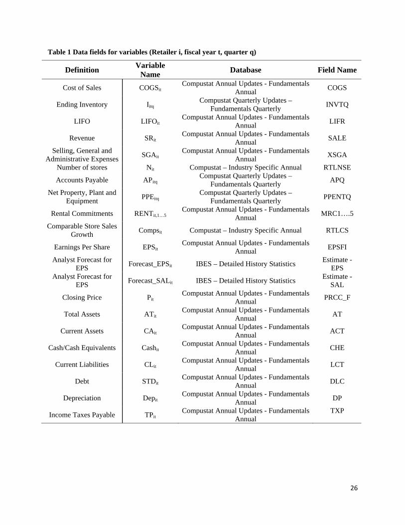
4.1 Definition of Variables

The following notations are used in the paper. For retailer i in fiscal year t, we denote as the total

sales revenue, as the cost of sales, as the selling, general and administrative expenses,

as the LIFO reserve, and , , … . as the rental commitments for the next

five years, ∆ as the change in current assets, ∆ as change in cash/cash equivalents, ∆ as

change in current liabilities, ∆ as change in debt included in current liabilities, ∆ as change in

income taxes payable, as depreciation and amortization expense, as the total assets and as

the total numbers of stores open for firm i at the end of fiscal year t. These are obtained from the

Compustat Annual Database. For firm i in fiscal year t and quarter q, we denote as the net

property, plant and equipment, as the accounts payable, and as the ending inventory. These are

obtained from the Compustat Quarterly Database.

Next we explain the adjustments that we make to the variables. The use of FIFO vs. LIFO

methods for valuing inventory produces artificial difference in the reported ending inventory and cost of

sales. Hence, to ensure that all retailers have similar inventory valuations, we add back LIFO reserve to

the ending inventory and subtract the annual change in LIFO reserve from the cost of sales. Similarly, the

value of PPE could vary depending on the values of capitalized leases and operating leases held by the

retailer. Hence, we first compute the present value of rental commitments for the next five years using

, , … . and then add it to the PPE to adjust uniformly for operating leases held by

a retailer. Here, we use a discount rate of d = 8% per year for computing the present value, and also verify

our results with d = 10%.We normalize some of the above variables by the number of retail stores in

order to avoid correlations that could arise due to scale effects caused by an increase or decrease in the

size of a firm. We calculate accruals based on Sloan (1996). Refer to Table 1 for the relevant data fields in

the Compustat Database. Using these data and adjustments, we calculate the following variables for each

firm i in fiscal year t and fiscal quarter q:

Average cost-of-sales per store:     ⁄

Average inventory per store: ∑  

Gross Margin:    ⁄

Average SGA per store: ⁄

Average capital investment per store: ∑   ∑

Store growth: ⁄

10  

Accounts payable to inventory ratio: ∑ 4⁄ ∑ 4⁄  

Accruals: 

∆  ∆   ∆  ∆ ∆ /       2⁄

The variables obtained after taking the logarithm are denoted by their respective lowercase letters, i.e.,

csit, isit, gmit, sgasit, capsit, git, and piit. In addition, we refer to comparable store sales as , actual

earnings per share as and closing share price as . All three values are obtained from the

Compustat Annual Database. Finally, we also obtained individual sell side analysts’ forecasts for

Earnings Per share (EPS) and Sales (SAL) from Institutional Brokers Estimate System (I/B/E/S), and

stock market returns from CRSP.

4.2 Data Description

We start with the entire population of U.S. retailers that have reported at least one year of financial

information during the period 1993-2009. The U.S. Department of Commerce classifies the retailers into

eight different categories, identified by the two-digit SIC code as follows: Lumber and other building

materials dealers (SIC: 52); general merchandise stores (SIC: 53); food stores (SIC: 54); eating and

drinking places (SIC: 55); apparel and accessory stores (SIC: 56); home furnishing stores (SIC: 57);

automotive dealers and service stations (SIC: 58) and miscellaneous retail (SIC: 59).

We exclude retailers in the categories eating and drinking places and automotive dealers and service

stations from our study as they contain significant service component to their business. There were 670

retailers that reported at least one year of data to the U.S. Securities and Exchange Commission (SEC) for

these years. Since data on the number of stores are sparsely populated in Compustat for the period prior to

1999, we obtain store data from Compustat starting from the year 1999 and supplement them with hand

collected data for the period before 1999. We find that 208 retailers did not report any store information.

To enable us to perform a longitudinal analysis, we only consider retailers that had atleast five years of

consecutive data. After removing several observations that had missing data for the variables required for

our analysis, we find that 369 of the 462 were left for further analysis. Further we eliminated foreign

retailers that are listed as American Depository Receipt (ADR) in the U.S. stock exchanges and also

removed jewelry firms from the miscellaneous retail sector as their inventory levels could be driven by

commodity prices and other macroeconomic conditions not captured by our model.

Inventory changes could also happen due to changes in foreign exchange rates, mergers &

acquisitions (M&A), and discontinued operations. For some companies, these changes could be

substantial. However, retailers do not report these changes separately. Hence, we identify firms that may

have undergone substantial changes in inventory due to these reasons in the following way. We follow

11  

Lundholm et al. (2010) to identify retailers with non-zero values of AQC and DO from Compustat3. We

find that about 35% of observations in our population of retailers from 1993 – 2009 had these values

populated with non-zero values. The values of AQC and DO have a wide range and depend on the relative

firm size. Hence, we normalize AQC and DO by total revenue and drop observations which are more than

3 standard deviations away from the mean as we expect these observations are likely to be cases wherein

inventory could have undergone substantial changes due M&A and discontinued operations. We also

identified retailers with non-zero values of PIFO from Compustat4 to account for retailers whose income

was affected substantially due to changes in foreign exchange rates and find that about 18% of the

observations in our population of retailers from 1993 – 2009 had this variable populated with a non-zero

value. We followed a similar procedure as above to drop observations with extreme values of PIFO as we

expect these would be cases where inventory changes may have been significantly impacted due to

fluctuations in foreign exchange rates. These data adjustments lead to a loss of 4% of observations from

our population of retailers from 1993-2009. Finally, some retailers may combine part of their selling,

general, and administrative expenses with cost of goods sold; we identify 15 such firm-year observations

in the period of 1993-2009 using the data code xsga_dc which is populated as “4” in such cases and drop

them from our analysis. We combine SIC 52 and SIC 57 as SIC 52 has a smaller number of firms and is

closest in match to SIC 57. After removing observations with missing data and making the above

adjustments, the resulting dataset had 323 retailers across 5 retail segments, viz. Apparel and Accessory

Stores, Food Stores, General Merchandise Stores, Home and Lumber, and Miscellaneous Retail Stores.

This resulted in 2653 observations for the period of 1993 – 2009.

We choose the six year time period from 2004-2009 as our test sample for analyzing the relationship

between abnormal inventory growth and one year ahead earnings. We have 136 retailers and 583 firm-

year observations in this sub-sample. Of the 136 retailers, we find that 125 retailers had reported

comparable store sales data yielding 519 firm-year observations. To determine the economic significance

of our results, we conduct further analysis with analysts’ forecasts and stock market data. We found

individual analysts’ forecasts of EPS were available for 446 of the 583 observations from I/B/E/S and

obtained stock market returns data for these 446 observations from CRSP. We provide further details on

these data in §7.

                                                            3 The definition for AQC in Compustat is given as “This item represents cash outflow of funds used for and/or the costs relating to acquisition of a company in the current year or effects of an acquisition in a prior year carried over to the current year.” The definition for DO in Compustat is given as “This item represents the total income (loss) from operations of a division discontinued or sold by the company and the gain (loss) on disposal of the division, reported after income taxes”. 4 The definition for this variable in Compustat is given as "This item represents the income of a company's foreign operations before taxes as reported by the company."

12  

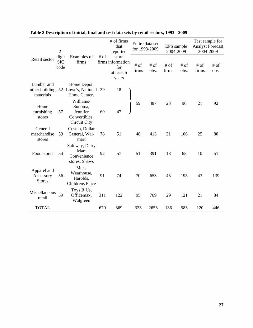
The number of retailers in each segment and distribution of retailers are given in Table 2. Summary

statistics for all variables used in our analysis is as shown in Table 3.

5. Methodology

In this section, we describe the methodology used to measure abnormal change in inventory levels. It is

customary in the operations management literature to determine the normal or expected changes in

inventory level based on expectation models for inventory levels for retailers. Deviations of actual

inventory levels from such expected inventory levels are then expected to serve as benchmarking metrics.

We use the expectation model from Kesavan et al. (2010) to measure abnormal inventory growth

for retailers. We use this model since it subsumes many of the factors identified in past research and it

was found to be useful in the context of sales forecasting. This model uses a log-log specification where

the inventory per store for a retailer in a given fiscal year depends on firm-fixed effect ( ), inventory per

store in the previous fiscal year ( , ), contemporaneous and lagged cost-of-goods-sold per store

( , , ), gross margin ( ), lagged accounts payable to inventory ratio ( , ), store growth

( ) and lagged capital investment per store ( , ) for that retailer. Using lower-case letters to

denote the logarithm of these variables, the logged inventory per store for retailer i in fiscal year t is given

as:

                                                                           1a

Where is a column vector of all right hand side explanatory variables;

1, , , , , , , and is the row vector of the corresponding

coefficients; , , , ,   , ,  ,   ′ and is the firm fixed effect.

First-differencing the above equation gets rid of the firm fixed-effect and yields the following

growth model:

∆ ∆ Δ                                                                        1b

Here denotes the change in logged variable in fiscal year t from fiscal year t-1.

One may treat all of the coefficients in the above regression as being firm specific, i.e. allow

the sensitivity of inventory per store to different factors such as cogs per store, gross margin, capital

investment per store etc. to vary from retailer to retailer. However, in order to estimate such a model, we

would need a long time-series of observations for each retailer. Since we use annual data in our analysis

we would need several decades of data for each retailer to estimate such a model. To overcome the

paucity of data, we assume that all firms in a given segment are homogenous, i.e. we assume that the

coefficients are same for all retailers within a given segment and estimate these coefficients at the

segment level. Thus our estimation equation is:

  ∆ , ∆                                                                          1c

13  

Where s(i) denotes the corresponding segment specific coefficients for firm i.

We can now obtain the expected logged inventory growth from the above equation,  , and

then compute abnormal inventory growth in the following way. Let 1 denote the actual

inventory per store growth and       1 1 denote the abnormal

inventory per store growth or, in short, abnormal inventory growth for a retailer i in fiscal year t. We

estimate (1c) and use the coefficients to compute abnormal inventory growth. Thus,   0 implies

that the retailer i has abnormally high inventory growth while   0 implies that the retailer i has

abnormally low inventory growth compared to the norm of the segment to which the retailer belongs to,

after controlling for firm-level differences.

Kesavan et al. (2010) show that historical gross margin contains information valuable to forecast

sales. Further they show that inventory and gross margin are highly correlated for retailers, so we

calculate abnormal change in gross margin in a similar manner as AIG and use it as a control variable in

our analysis. Similar to equation 1c, the first differenced equation for gross margin can be written as:

  ∆ , Δ                                                                          2

Where ∆ 1, Δ , Δ , Δ . We calculate abnormal change in gross margin for retailer i in

fiscal year t as       1 1 .

Next, we explain the data used to obtain   from (1c) which is then used to predict earnings

in fiscal year t. We use data till fiscal year t-2 to estimate (1c). We avoid data from fiscal year t-1 in the

estimation since firms announce their financial results at different times of the year that could lead to a

potential look-ahead which could bias our results about the relationship between AIG and one-year ahead

earnings. Once a retailer’s financial results are announced for fiscal year t-1, we use the coefficient

estimates to measure the     for that retailer. We follow this process for all retailers in our test

sample, i.e., t=2004, 2009. We follow a similar approach to obtain .

We considered two different techniques to estimate equations (1c) and (2). We used the

instrument variable generalized least squares (IVGLS) method used in Kesavan et al. (2010) to estimate

the equations and also used a simpler single equation technique, a Generalized Least Squares method

(GLS), to estimate these equations. We found the results to be similar. Since the IVGLS method requires

defining an additional equation containing new variables, we choose to report the results of the GLS

technique that is simpler to implement and explain. The GLS method handles heteroskedasticity and

panel specific auto-correlation in the data.

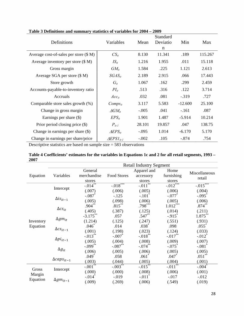
Table 4 reports sample results of estimation of equations (1c) and (2) using data from 1993 –

2007. These coefficient estimates were then used to calculate AIG and ACGM for fiscal year 2008 that

14  

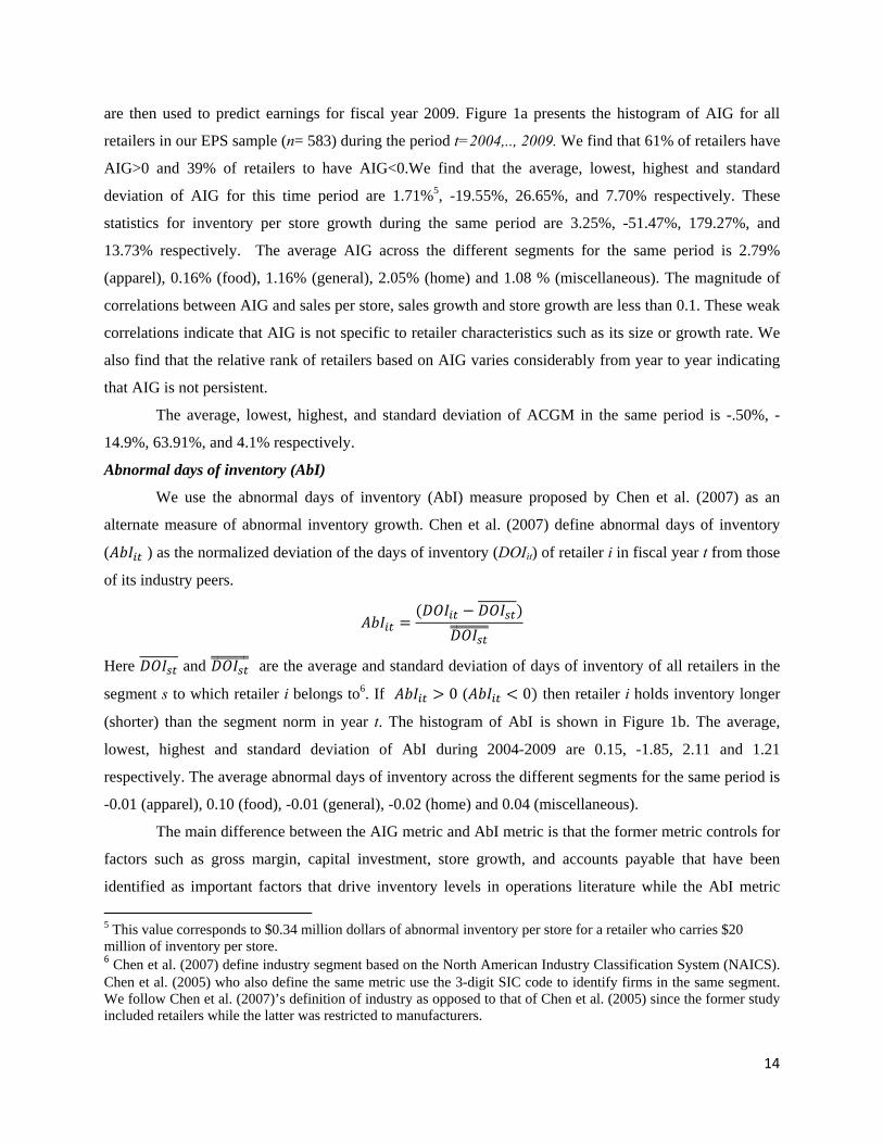
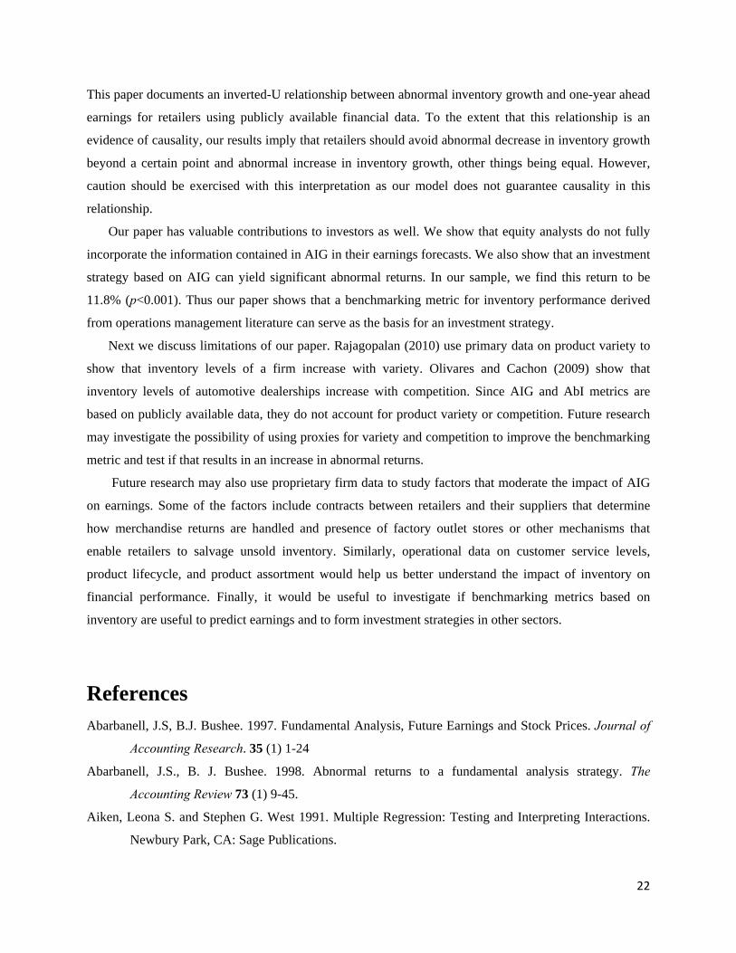
are then used to predict earnings for fiscal year 2009. Figure 1a presents the histogram of AIG for all

retailers in our EPS sample (n= 583) during the period t=2004,.., 2009. We find that 61% of retailers have

AIG>0 and 39% of retailers to have AIG<0.We find that the average, lowest, highest and standard

deviation of AIG for this time period are 1.71%5, -19.55%, 26.65%, and 7.70% respectively. These

statistics for inventory per store growth during the same period are 3.25%, -51.47%, 179.27%, and

13.73% respectively. The average AIG across the different segments for the same period is 2.79%

(apparel), 0.16% (food), 1.16% (general), 2.05% (home) and 1.08 % (miscellaneous). The magnitude of

correlations between AIG and sales per store, sales growth and store growth are less than 0.1. These weak

correlations indicate that AIG is not specific to retailer characteristics such as its size or growth rate. We

also find that the relative rank of retailers based on AIG varies considerably from year to year indicating

that AIG is not persistent.

The average, lowest, highest, and standard deviation of ACGM in the same period is -.50%, -

14.9%, 63.91%, and 4.1% respectively.

Abnormal days of inventory (AbI)

We use the abnormal days of inventory (AbI) measure proposed by Chen et al. (2007) as an

alternate measure of abnormal inventory growth. Chen et al. (2007) define abnormal days of inventory

( ) as the normalized deviation of the days of inventory (DOIit) of retailer i in fiscal year t from those

of its industry peers.

Here and are the average and standard deviation of days of inventory of all retailers in the

segment s to which retailer i belongs to6. If 0 ( 0 then retailer i holds inventory longer

(shorter) than the segment norm in year t. The histogram of AbI  is shown in Figure 1b. The average,

lowest, highest and standard deviation of AbI during 2004-2009 are 0.15, -1.85, 2.11 and 1.21

respectively. The average abnormal days of inventory across the different segments for the same period is

-0.01 (apparel), 0.10 (food), -0.01 (general), -0.02 (home) and 0.04 (miscellaneous).

The main difference between the AIG metric and AbI metric is that the former metric controls for

factors such as gross margin, capital investment, store growth, and accounts payable that have been

identified as important factors that drive inventory levels in operations literature while the AbI metric

                                                            5 This value corresponds to $0.34 million dollars of abnormal inventory per store for a retailer who carries $20 million of inventory per store. 6 Chen et al. (2007) define industry segment based on the North American Industry Classification System (NAICS). Chen et al. (2005) who also define the same metric use the 3-digit SIC code to identify firms in the same segment. We follow Chen et al. (2007)’s definition of industry as opposed to that of Chen et al. (2005) since the former study included retailers while the latter was restricted to manufacturers.

15  

does not. However, the use of lagged variables in the regression used to estimate AIG means that we need

at least three years of data to measure AIG for a retailer. On the other hand, the AbI metric can be

computed even for a retailer that has just one year of data. We use both metrics to test the relationship

between abnormal inventory growth and one-year ahead earnings.

6. Results

In this section, we discuss the results of our statistical tests of the relationship between AIG and one-

year ahead earnings. Several researchers in accounting have used a first order autoregressive model for

change in one-year ahead earnings. We adopt the same model to test the relationship between AIG and

one-year ahead earnings. Accounting literature has also found that accruals, defined as the difference

between net income and operating cash flows, predict one-year ahead earnings (Sloan 1996). Since one of

the components of accruals is change in inventory, we use accruals as a control variable to examine if

AIG has additional information over that contained in accruals to predict earnings. This gives us the

following model to test the relationship between AIG and one-year ahead earnings:

∆ 1        ∆ 1 ∆     

                                                                                                                                                    3

Here, ∆ 1  denotes change in EPS deflated by previous fiscal year’s ending stock price to

homogenize firms when firms are drawn from a broad range of sizes (Durtschi and Easton, 2005). We use

a full set of year dummies ( ) to account for macroeconomic factors that may impact earnings of all

retailers. We use coefficient estimates of and to determine the relationship between AIG and

change in one year ahead earnings.

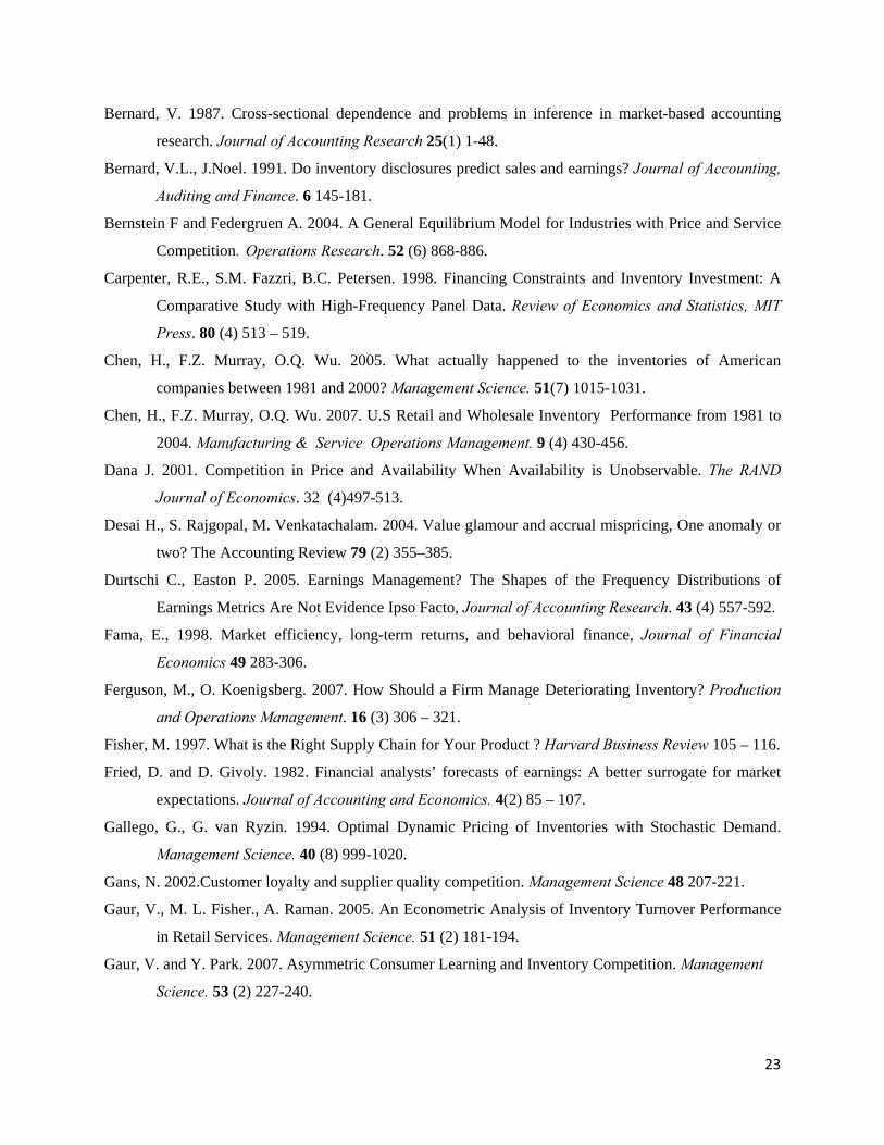
Model 1 in Table 5 reports the results for the base model, i.e. a first order autoregressive model of

EPS with accruals. Consistent with the accounting literature, we find that accruals have predictive power

over one-year ahead earnings. Model 2 gives the estimated coefficients of Equation 3. We find that the

coefficients of   and are negative and significant (p<0.001) and provide support for an

inverted-U relationship between AIG and change in one-year ahead EPS. We perform a Wald test to

confirm that the addition of   and improves the fit of our model (p<0.001). We use the

coefficient estimates ( , from Model 2 to graphically illustrate the inverted-U relationship

between AIG and change in one-year ahead earnings as shown in Figure 2. The mean AIG in our sample

is .017 and the standard deviation is 0.07. At the mean, the impact of increasing AIG by 0.01 leads to a

decrease in EPS of 0.2 cents. At a higher level of distribution, corresponding to mean plus 2 times the

standard deviation, increasing AIG by 0.01 leads a decrease in EPS of 0.7 cents. At a lower level of

distribution, (corresponding to mean minus two times the standard deviation), further decreasing AIG by

0.01 leads to a decrease in EPS of 0.3 cents.

16  

To ensure that outliers are not driving the inverted-U relationship, we follow Aiken and West

(1991) to statistically test this relationship. Aiken and West (1991) recommend performing tests for the

significance of slopes spanning observations on either side of the inflexion point and verify the change in

signs of the slopes. The inflexion point occurs at a value of -0.049 /2 which is less than

one standard deviation away from the mean and well within the range of our sample, [-0.195, 0.267]. We

find that 16% of our observations lie to the left of the inflexion point. We perform t-tests of simple slopes

using coefficient estimates of (3) and the results are reported in Table 6. Since the simples slopes at

values of AIG that are two standard deviations below mean and above mean are both statistically

significant and opposite in signs, we can conclude that the inverted-U relationship between AIG and one-

year ahead earnings is supported within the range of our data and not driven by outliers.

There are two attributes of the inverted-U relationship that we further elaborate on. First, the

inflexion point occurring at a value less than zero is interesting. Since our results are picking up the

dominant effect (as we cannot control for service level), we conjecture that the region [-0.049, 0] is

dominated by retailers who became leaner. That is, these retailers were able to reduce their inventory

levels without substantial reduction in service level. We conjecture that the region AIG<-0.049 is

dominated by retailers whose inventory levels declined so much that the accompanying decline in service

level hurt their one-year ahead earnings. To ensure that this result is not an artifact of the AIG metric, we

re-test Model 2 by substituting the AIG metric with AbI metric from Chen et al. (2007) and find

qualitatively similar results. The coefficients of   and are -0.006 and -0.007 (p<0.001)

respectively indicating the existence of an inverted-U shape relationship between AbI and change in one-

year ahead earnings. Similar to the results obtained with the AIG metric, we find that the inflexion point

is negative and lies within one standard deviation of the mean. The values of the inflexion point,

minimum, and maximum values of AbI are -0.43, -1.85, and 2.11 respectively. Thus our results appear to

be robust to the method used to compute abnormal inventory carried by retailers.

Second, consistent with Chen et al. (2007) who examined long-term stock market returns of

retailers, we find that our strongest results are for retailers with abnormally high inventory growth who

have poor subsequent performance. There are likely to be some retailers in this region (AIG>0) who were

able to increase service level such that the new service level is closer to the optimal service level and

found a subsequent increase in profitability. However, those retailers appear to be dominated by retailers

who had excess inventory.

We perform several robustness checks to confirm the inverted-U relationship. First, we control

for ACGM as Kesavan et al. (2010) show that this variable contains information useful to predict sales.

The correlation between AIG and ACGM is low (ρ=-0.18) and not significant. We also compute the

variance inflation factor (VIF) between AIG and ACGM for Model 3 and find it to be 1.3. This rules out

17  

any multicollinearity issues arising due to including these variables together in an equation as the VIF is

less than 10 (Maddala 2001). The results, as shown in Model 3 in Table 5, continue to show the inverted-

U relationship. Second, we add segment dummies to Model 3 and the estimation results are as shown in

Model 4. Our conclusions about the inverted-U relationship remain unchanged with the addition of these

variables.

Because AIG predicts sales (Kesavan et al. 2010) and earnings are a function of sales, we want to

determine if the relationship between AIG and earnings are driven only by AIG’s ability to predict sales

or if there are additional reasons why AIG might predict earnings. As we argue in §3, AIG might also

predict higher expenses such as advertising costs to clear merchandise, holding costs, and inventory write-

downs. Since these expenses are not readily available as separate line items in retailers’ income statement

we test this indirectly in the following way. We add one-year ahead comparable store sales ( ) to

Model 4 to control for changes in EPS due to change in sales for that retailers in the following way:

∆ 1        ∆ 1     

  ∆     ,                                         4

Thus, significance of AIG would indicate that it contains information about future expenses that would be

useful to predict one-year ahead earnings for retailers. Models 5 and 6 in Table 7 report the results of the

base model and results from equation 4. We find that both the linear term and the quadratic terms of AIG

are significant (p<0.001), even after controlling for contemporaneous values of comparable store sales,

indicating that AIG predicts earnings for retailers due to its ability to predict sales and expenses for

retailers. We also replace comparable store sales in period t with sales growth in that period and obtain

similar results (not reported).

7. Economic Significance of Information contained in AIG

In this section, we investigate the economic significance of our finding. First, we examine if equity

analysts take the information contained in AIG into account when generating their earnings forecasts.

Second, we test if stock prices incorporate this information. The former test would show if even

sophisticated investors could benefit from knowing the information contained in AIG and the latter would

indicate if AIG can form the basis for an investment strategy.

7.1 Do equity analysts ignore information in abnormal inventory growth in

EPS forecasts?

We examine if equity analysts ignore information contained in AIG or not in the following way.

Analysts issue earnings forecasts at different times during a year and revise those forecasts as more

information becomes available. These forecasts are time stamped with the dates that they are issued.

Since the financial information for the previous fiscal year are released on the earnings announcement

18  

date (EAD), the information required to compute AIG for a retailer is available after its EAD. If analysts’

incorporate the information from lagged AIG, then their forecasts issued subsequent to EAD should not

generate errors that can be predicted by lagged AIG. On the other hand, if they do not incorporate this

information then lagged AIG will have predictive power over their forecast errors.

Our tests are conducted using the IBES detailed (median) forecasts of annual EPS. We perform

this analysis using data obtained for fiscal years 2004-2009. We consider analysts’ earnings forecasts for

the forthcoming fiscal year issued after EAD of the prior fiscal year. In some cases, analysts might have

to wait till the retailers file their 10-K statement with SEC to have access to those retailer’s financial

statements. To be conservative, we drop any analyst forecasts made before the SEC filing date as well.

We obtain SEC filing date for each retailer from Morningstar Document Research that is accessible from

http://www.10kwizard.com/. If multiple forecasts are made by an analyst for a retailer, we use the most

recent forecast as it should contain the latest information available to them.

We find that analysts’ forecasts were available for 446 observations out of the 583 overall

observations. For each firm-year, we determine the median of analysts’ forecasts made for each of the m=

1 to 12 months after EAD for fiscal year t-1 and use it as consensus forecasts to generate analysts’

consensus forecast error. We compute forecast errors by subtracting consensus EPS forecast from realized

EPS. We also deflate the forecast error by the previous fiscal year’s ending stock price (Gu and Wu

2003). The average, standard deviation, minimum, and maximum deflated analysts’ forecast error

between 2004-2009 are -.005, .036, -.384, and .137 respectively. The average forecast error of -.005

shows that analysts are optimistic on average, which is consistent with prior accounting literature.

Next we statistically test if analysts’ forecast errors are biased are predicted by lagged AIG by

running the following regression:

  , ,   ψ (5)

Here,  is the deflated forecast error of analysts’ consensus forecast generated m months before end

of fiscal year t for retailer i. is the bias that is common to all retailers, is the bias that is specific to a

given fiscal year, is that bias that is correlated with previous year’s AIG; and is the bias that is

correlated with previous year’s ACGM. is the vector of control variables that were found to be

related to forecast bias in the accounting literature (Gu and Wu 2003). These include dispersion among

analysts’ forecasts, analyst coverage, market value, unexpected earnings from a seasonal random walk

model, and a dummy variable to capture ex-ante expectation of loss in earnings.

We estimate (5) using the GLS technique. Table 8 provides the formal statistical test of the relation

between analysts’ forecast errors and lagged AIG. We find that the bias in analysts’ forecasts due to AIG

continues to remain significant (p<0.1) up to 6 months from EAD for the prior fiscal year as shown in

Table 8. The magnitude of the reported coefficients may be interpreted in the following way. Consider the

19  

forecasts made m= 6 months after EAD for the prior fiscal year (m = 6 in table 8). We find that the

coefficient of AIG is -.019 (p<0.1). This implies that for an average retailer with a share price of $28.101

(mean share price in our sample), a one standard deviation increase in AIG is associated with 4.11 cents

increase in analysts’ forecast error. We also confirm that the direction and significance of our control

variables are consistent with prior accounting literature (Gu and Wu 2003).

Next, we want to determine if our result that AIG predicts bias in analysts EPS forecasts is driven due

to analysts failing to incorporate information contained in AIG to predict sales, as shown by Kesavan et

al. (2010), or to predict expenses as well. We do so by picking analysts’ sales forecasts made m=6 months

after EAD for prior fiscal year (column 3, table 8). Sales forecasts were available for only 387 out of 446

observations in our sample. We add contemporaneous error in analysts’ sales forecasts to equation 5 for

this sample (m = 6) and find that AIG continues to remain a significant predictor of bias in analysts’

forecasts of EPS (p<0.1). We obtain consistent results for m=1 and 3 months as well where the results are

stronger (p<0.05).

To summarize, our results show that analysts fail to incorporate information in AIG to predict

earnings. These results not only support the results from Kesavan et al. (2010) but add to it by showing

that analysts fail to incorporate the information contained in AIG useful to forecast expenses as well.

7.2 Does an investment strategy based on AIG yield abnormal returns?

In this section, we examine whether investments based on AIG can yield abnormal returns. We

follow the methodology used in Abarbanell and Bushee (1998) and Desai et al (2004) to perform this

analysis. This methodology can be used to determine the abnormal returns to a zero-investment strategy

based on AIG and other control variables. We use accruals, inventory growth, and book-to-market as

control variables for the following reasons. Sloan (1996) showed that investment strategies based on

accruals yields significant abnormal returns. Since accruals are comprised of many components, Thomas

and Zhang (2002) test the strength of each of those components and find that the inventory growth

component has the highest explanatory power. We are motivated to examine if investment strategy based

on AIG would generate incremental abnormal returns after controlling for accruals and inventory growth.

Finally, we also control for book-to-market as it is a proxy for whether a firm is a value stock or not

(Desai et al. 2004).

This methodology involves dividing firms in to different portfolios based on quintile ranks of AIG

and quintile ranks of each of the control variables. An important consideration in the construction of these

portfolios is that all information required to construct the portfolios for a given fiscal year are available at

the time point when the portfolio is created. Since firms file their 10-K statements with SEC at different

time points in the year, the information required to construct a portfolio comprising of all the retailers

20  

becomes available at different points in time. In our sample, we find that the month of April had the most

number of SEC filings (245), followed by March (83) and May (52). The rest of the months had fewer

than 20 filings. To ensure that all firms in our portfolio are aligned in calendar time such that their 10-K

statements are filed in the same month, we include only firms that file their 10-K statements in April.

Thus our portfolios are created on May 1 and we compute the buy-and-hold abnormal returns for the 12

month period from thereon.

We measure the size-adjusted buy-and-hold abnormal return (BHAR) of each of the stock in our

sample in the following way (Kothari and Warner 2007). The for firm i cumulated for a period of

12 months for fiscal year t, beginning from May of the prior fiscal year is:

  1   1

Where is the stock return of firm i in month m and is the return of the value-weighted

portfolio of firms in the CRSP size decile to which this firm belongs for that fiscal year. The size deciles

are obtained from the distribution of market values of all NYSE/AMEX firms at the beginning of the

fiscal year.

Next we compute the quintile ranks based on lagged AIG for each of the firms in each of the fiscal

years 2004-2009, and then scale those ranks to obtain new variable . We illustrate using fiscal

year 2004 as an example. First, we rank firms from 0 to 4 based on the quintile rank of . Retailers

with rank of zero (four) are those firms whose AIG were low (high) enough to belong to the bottom (top)

quintile in 2003. Next we divide the ranks by 4 to obtain . We repeat the above procedure to

obtain variables , , which are the scaled quintile ranks based on lagged

accruals, lagged inventory growth, and lagged book-to-market respectively. The values of each of these

scaled variables will lie between 0 and 1.

After creating all the variables, we run a number of regressions of against different

combinations of , , , and , after controlling for year-fixed effects.

The coefficients on each of the variables can be interpreted as the abnormal return to a zero investment

strategy in the respective variable. This test of significance of these coefficients has been found to

overcome bias that might otherwise occur due to cross-sectional correlation of the size-adjusted return

metric (Bernard 1987).

The regression results are reported in Table 9. First, consider models M1a, M1b, and M1c. Model

M1a shows that a zero investment strategy based on accruals would yield an abnormal return of 10.1%

(p<0.001). This result is consistent with that reported in Sloan (1996). Similar analysis, as shown in

Model 1b, shows that the abnormal returns to AIG is 11.8% (p<0.001). Next, we consider accruals and

AIG together in Model 1c and find that the incremental returns of AIG decreases from 11.8% to 10.8%

21  

but continues to remain significant (p<0.001). Our results show that an investment strategy based on AIG

would produce abnormal returns. Furthermore, we find that the information content in AIG is not

subsumed in accruals.

Next we want to determine if AIG contains more information than inventory growth metric, defined

as change in total inventory scaled by average total assets (Thomas and Zhang 2002). So, we run model

M2 where we replace accruals ( ) in M1a by inventory growth ( . Consistent with

Thomas and Zhang (2002), we find that abnormal returns to inventory growth to be significant (p<

0.001). Finally, we run full Model M3 which includes all the variables. We find that incremental return to

AIG is 10.3% (p<0.001). However, the incremental returns to inventory growth are no longer significant;

this is as expected since inventory growth is a component of accruals. Thus we add to the results of

Thomas and Zhang (2002) by showing that it is the abnormal component of inventory growth, not the

normal component, which generates abnormal returns.

We also perform additional robustness tests to validate our findings. First, we ran cross-sectional

regressions of the full model for each of the six years (2004-2009) and find that abnormal returns to AIG

are significant (p<0.1) in each of those years and they vary between 3.91% (p<0.1) and 12.9% (p<0.001).

Similarly, we find abnormal returns to accruals also to be significant (p<0.1) for all 6 years while the

abnormal returns to inventory growth is significant (p<0.1) in four of the six years.

Next, we increase our sample size by considering retailers whose SEC filing dates were in March

(n=83) and May (n=52) in addition to those who filed in April (n=245). Our number of observations

increases to 380. In order to ensure that all the information required to create portfolios are available at

the time of creating the portfolio, our holding period starts from June 1 and continues for 12 months.

Thus, we would wait for atleast 2 months for retailers who release their 10K statements in March and

atleast 1 month for those who release their 10K statements in April before including them in our portfolio.

We find qualitatively similar results as in Table 9, i.e. abnormal returns to a zero-investment strategy in

AIG continue to be significant. For example, when we run the full Model M5 in this sample, we find the

abnormal returns to AIG, accruals, and inventory growth to be 8.1%, 7.2% and 2.6% respectively. The

abnormal returns to AIG are significant at 5% level while the abnormal returns to inventory growth are

not significant.

We also test the robustness of this finding using the Ibbotson-RATS procedure that we briefly explain

in the Appendix (see Kothari and Warner 2007 for more details). This approach allows us to estimate the

abnormal returns of the hedge portfolios using the three-factor Fama-French model. Using this approach,

we find abnormal returns to AIG, accruals, and inventory growth are 11.65%; 6.57%; and 3.86%

respectively. Thus our results are robust to the method used to estimate abnormal returns.

8. Conclusion, Limitations, and Future Work

22  

This paper documents an inverted-U relationship between abnormal inventory growth and one-year ahead

earnings for retailers using publicly available financial data. To the extent that this relationship is an

evidence of causality, our results imply that retailers should avoid abnormal decrease in inventory growth

beyond a certain point and abnormal increase in inventory growth, other things being equal. However,

caution should be exercised with this interpretation as our model does not guarantee causality in this

relationship.

Our paper has valuable contributions to investors as well. We show that equity analysts do not fully

incorporate the information contained in AIG in their earnings forecasts. We also show that an investment

strategy based on AIG can yield significant abnormal returns. In our sample, we find this return to be

11.8% (p<0.001). Thus our paper shows that a benchmarking metric for inventory performance derived

from operations management literature can serve as the basis for an investment strategy.

Next we discuss limitations of our paper. Rajagopalan (2010) use primary data on product variety to

show that inventory levels of a firm increase with variety. Olivares and Cachon (2009) show that

inventory levels of automotive dealerships increase with competition. Since AIG and AbI metrics are

based on publicly available data, they do not account for product variety or competition. Future research

may investigate the possibility of using proxies for variety and competition to improve the benchmarking

metric and test if that results in an increase in abnormal returns.

Future research may also use proprietary firm data to study factors that moderate the impact of AIG

on earnings. Some of the factors include contracts between retailers and their suppliers that determine

how merchandise returns are handled and presence of factory outlet stores or other mechanisms that

enable retailers to salvage unsold inventory. Similarly, operational data on customer service levels,

product lifecycle, and product assortment would help us better understand the impact of inventory on

financial performance. Finally, it would be useful to investigate if benchmarking metrics based on

inventory are useful to predict earnings and to form investment strategies in other sectors.

References Abarbanell, J.S, B.J. Bushee. 1997. Fundamental Analysis, Future Earnings and Stock Prices. Journal of

Accounting Research. 35 (1) 1-24

Abarbanell, J.S., B. J. Bushee. 1998. Abnormal returns to a fundamental analysis strategy. The

Accounting Review 73 (1) 9-45.

Aiken, Leona S. and Stephen G. West 1991. Multiple Regression: Testing and Interpreting Interactions.

Newbury Park, CA: Sage Publications.

23  

Bernard, V. 1987. Cross-sectional dependence and problems in inference in market-based accounting

research. Journal of Accounting Research 25(1) 1-48.

Bernard, V.L., J.Noel. 1991. Do inventory disclosures predict sales and earnings? Journal of Accounting,

Auditing and Finance. 6 145-181.

Bernstein F and Federgruen A. 2004. A General Equilibrium Model for Industries with Price and Service

Competition. Operations Research. 52 (6) 868-886.

Carpenter, R.E., S.M. Fazzri, B.C. Petersen. 1998. Financing Constraints and Inventory Investment: A

Comparative Study with High-Frequency Panel Data. Review of Economics and Statistics, MIT

Press. 80 (4) 513 – 519.

Chen, H., F.Z. Murray, O.Q. Wu. 2005. What actually happened to the inventories of American

companies between 1981 and 2000? Management Science. 51(7) 1015-1031.

Chen, H., F.Z. Murray, O.Q. Wu. 2007. U.S Retail and Wholesale Inventory Performance from 1981 to

2004. Manufacturing & Service Operations Management. 9 (4) 430-456.

Dana J. 2001. Competition in Price and Availability When Availability is Unobservable. The RAND

Journal of Economics. 32 (4)497-513.

Desai H., S. Rajgopal, M. Venkatachalam. 2004. Value glamour and accrual mispricing, One anomaly or

two? The Accounting Review 79 (2) 355–385.

Durtschi C., Easton P. 2005. Earnings Management? The Shapes of the Frequency Distributions of

Earnings Metrics Are Not Evidence Ipso Facto, Journal of Accounting Research. 43 (4) 557-592.  

Fama, E., 1998. Market efficiency, long-term returns, and behavioral finance, Journal of Financial

Economics 49 283-306.

Ferguson, M., O. Koenigsberg. 2007. How Should a Firm Manage Deteriorating Inventory? Production

and Operations Management. 16 (3) 306 – 321.

Fisher, M. 1997. What is the Right Supply Chain for Your Product ? Harvard Business Review 105 – 116.

Fried, D. and D. Givoly. 1982. Financial analysts’ forecasts of earnings: A better surrogate for market

expectations. Journal of Accounting and Economics. 4(2) 85 – 107.

Gallego, G., G. van Ryzin. 1994. Optimal Dynamic Pricing of Inventories with Stochastic Demand.

Management Science. 40 (8) 999-1020.

Gans, N. 2002.Customer loyalty and supplier quality competition. Management Science 48 207-221.

Gaur, V., M. L. Fisher., A. Raman. 2005. An Econometric Analysis of Inventory Turnover Performance

in Retail Services. Management Science. 51 (2) 181-194.

Gaur, V. and Y. Park. 2007. Asymmetric Consumer Learning and Inventory Competition. Management

Science. 53 (2) 227-240. 

24  

Givoly, D., J. Lakonishok. 1984. The Quality of Analysts’ Forecasts of Earnings. Financial Analysts

Journal. 40 (5) 40 – 47.

Gu, Z., & Wu, J. 2003. Earnings skewness and analyst forecast bias. Journal of Accounting and

Economics. 35 5–29.

Hendricks, K.B., V.R. Singhal. 2005. Association between Supply Chain Glitches and Operating

Performance. Management Science. 51 (5) 695-711.

Hendricks, K.B., V.R. Singhal. 2009. Demand – Supply Mismatches and Stock Market Reaction:

Evidence from Excess Inventory Announcement. Manufacturing & Service Operations

Management. 11 (3) 509 - 524.

Kesavan, S. V. Gaur., A. Raman. 2010. Incorporating Price and Inventory Endogeneity in Firm Level

Sales Forecasting. Management Science. 56 (9) 1519 - 1533

Kothari, S. P., & Warner, J. B. 2007. Econometrics of event studies. In B. E. Eckbo (Ed.),

Handbook of Corporate Finance: Empirical Corporate Finance. North Holland: Elsevier.

Lai, R. 2006. Inventory Signals, Harvard NOM Research Paper Series No. 05-15. Boston, MA: Harvard

Business School. 

Lee H.L., V. Padmanabhan, S. Whang. 1997. Information Distortion in a Supply Chain: The Bullwhip

Effect. Management Science. 43 (4) 546-558.

Lundholm, R., S. McVay. 2010. Forecasting Sales: A Model and Some Evidence from the Retail

Industry. Working paper, University of Michigan.

Maddala, G.S. 2001. Introduction to Econometrics. John Wiley & Sons, New York.

Makridakis, S., and S. C. Wheelwright. 1987. The Handbook of Forecasting: A Manager’s Guide. John

Wiley & Sons, New York.

Mitchell, M., and E. Stafford 2000. Managerial decisions and long-term stock price performance, Journal

of Business 73 287-329.

Olivares, M. G. Cachon. 2009. Competing Retailers and Inventory: An Empirical Investigation of General

Motors' Dealerships in Isolated U.S. Markets. Management Science. 55 (9) 1586 - 1604

Rajagopalan, S. 2010. Factors driving inventory levels at US retailers. Working paper.

Raman, A., V. Gaur., S. Kesavan. 2005. David Berman. Harvard Business School Case 605-081.

Rumyantsev, S. , S. Netessine. 2007. What Can be Learned from Classical Inventory Models? A Cross-

Industry Exploratory Investigation. Manufacturing & Service Operations Management. 9 (4) 409

– 429.

Sloan, R. 1996. Do stock prices fully reflect information in accruals and cash flows about future earnings?

The Accounting Review 71 289–315.

25  

Smith, S., D. Achabal. 1998. Clearance Pricing and Inventory Policies for Retail Chains. Management

Science. 44 (3) 285-300.

Stickney, C.P., R.L. Weil. 2003. Financial Accounting: An Introduction to Concepts, Methods, and Uses.

Thomson, South-Western.

Thomas, J.K., H. Zhang. 2002. Inventory Changes and Future Returns. Review of Accounting Studies.7

(2) 163 – 187.

Figure 1: Histograms of AIG and AbI

Figure 2: Impact of AIG on one-year ahead change in earnings per share (EPS1) 

 

The impact of AIG on one-year ahead earnings per share is measured using estimates of coefficients from Model 2 (table 5) in the following way, i.e., Impact .165 1.689

‐0.2

‐0.15

‐0.1

‐0.05

0

0.05

‐0.2 ‐0.1 0 0.1 0.2 0.3

AIG E

P

S

1 

26  

Table 1 Data fields for variables (Retailer i, fiscal year t, quarter q)

Definition Variable

Name Database Field Name

Cost of Sales COGSit Compustat Annual Updates - Fundamentals

Annual COGS

Ending Inventory Iitq Compustat Quarterly Updates –

Fundamentals Quarterly INVTQ

LIFO LIFOit Compustat Annual Updates - Fundamentals

Annual LIFR

Revenue SRit Compustat Annual Updates - Fundamentals

Annual SALE

Selling, General and Administrative Expenses

SGAit Compustat Annual Updates - Fundamentals

Annual XSGA

Number of stores Nit Compustat – Industry Specific Annual RTLNSE

Accounts Payable APitq Compustat Quarterly Updates –

Fundamentals Quarterly APQ

Net Property, Plant and Equipment

PPEitq Compustat Quarterly Updates –

Fundamentals Quarterly PPENTQ

Rental Commitments RENTit,1…5 Compustat Annual Updates - Fundamentals

Annual MRC1….5

Comparable Store Sales Growth

Compsit Compustat – Industry Specific Annual RTLCS

Earnings Per Share EPSit Compustat Annual Updates - Fundamentals

Annual EPSFI

Analyst Forecast for EPS

Forecast_EPSit IBES – Detailed History Statistics Estimate -

EPS Analyst Forecast for

EPS Forecast_SALit IBES – Detailed History Statistics

Estimate - SAL

Closing Price Pit Compustat Annual Updates - Fundamentals

Annual PRCC_F

Total Assets ATit Compustat Annual Updates - Fundamentals

Annual AT

Current Assets CAit Compustat Annual Updates - Fundamentals

Annual ACT

Cash/Cash Equivalents Cashit Compustat Annual Updates - Fundamentals

Annual CHE

Current Liabilities CLit Compustat Annual Updates - Fundamentals

Annual LCT

Debt STDit Compustat Annual Updates - Fundamentals

Annual DLC

Depreciation Depit Compustat Annual Updates - Fundamentals

Annual DP

Income Taxes Payable TPit Compustat Annual Updates - Fundamentals

Annual TXP

27  

Table 2 Description of initial, final and test data sets by retail sectors, 1993 - 2009

Retail sector

2-digit SIC code

Examples of firms

# of firms

# of firms that

reported store

information for

at least 5 years

Entire data set for 1993-2009

EPS sample 2004-2009

Test sample for Analyst Forecast

2004-2009

# of firms

# of obs.

# of firms

# of obs.

# of firms

# of obs.

Lumber and other building

materials 52

Home Depot, Lowe's, National

Home Centers 29 18

59 487 23 96 21 92 Home

furnishing stores

57

Williams-Sonoma, Jennifer

Convertibles, Circuit City

69 47

General merchandise

stores 53

Costco, Dollar General, Wal-

mart 78 51 48 413 21 106 25 80

Food stores 54

Safeway, Dairy Mart

Convenience stores, Shaws

92 57 51 391 18 65 10 51

Apparel and Accessory

Stores 56

Mens Wearhouse,

Harolds, Childrens Place

91 74 70 653 45 195 43 139

Miscellaneous retail

59 Toys R Us, Officemax, Walgreen

311 122 95 709 29 121 21 84

TOTAL 670 369 323 2653 136 583 120 446

28  

Table 3 Definitions and summary statistics of variables for 2004 – 2009

Definitions Variables Mean Standard Deviatio

n Min Max

Average cost-of-sales per store ($ M) CSit 8.130 11.341 .189 115.267

Average inventory per store ($ M) ISit 1.216 1.955 .011 15.118

Gross margin GMit 1.584 .225 1.121 2.613

Average SGA per store ($ M) SGASit 2.189 2.915 .066 17.443

Store growth Git 1.067 .162 .299 2.459

Accounts-payable-to-inventory ratio PIit .513 .316 .122 3.714

Accruals Accit .032 .081 -.319 .727

Comparable store sales growth (%) Compsit 3.117 5.583 -12.600 25.100

Change in gross margin GMit -.005 .041 -.161 .087

Earnings per share ($) EPSit 1.901 1.487 -5.914 10.214

Prior period closing price ($) Pit-1 28.101 19.857 .047 138.75

Change in earnings per share ($) EPSit -.095 1.014 -6.170 5.170

Change in earnings per share/price EPS1it-1 -.002 .105 -.874 .754

Descriptive statistics are based on sample size = 583 observations Table 4 Coefficients’ estimates for the variables in Equations 1c and 2 for all retail segments, 1993 – 2007

Retail Industry Segment

Equation Variables General

merchandise stores

Food Stores Apparel and

accessory stores

Home furnishing

stores

Miscellaneous retail

Inventory Equation

Intercept -.014**

(.007) -.018***

(.006) -.011**

(.005) -.012***

(.006) -.015***

(.004)

∆ -.087*

(.005) -.125 (.098)

-.101*

(.006) -.077*

(.005) -.095*

(.006)

∆ .904**

(.405) .815**

(.387) .798***

(.125) 1.012***

(.014) .874**

(.211)

∆ -3.175**

(1.214) .057

(.125) .547**

(.247) -.915*

(.551) 1.875**

(.931)

∆ .046*

(.001) .014

(.198) .038*

(.023) .098

(.124) .055*

(.033)

∆ -.013**

(.005) -.007*

(.004) -.018**

(.008) -.017**

(.009) -.012*

(.007)

∆ -.099**

(.006) -.087**

(.005) -.074**

(.006) -.075*

(.005) -.081*

(.005)

∆ .049*

(.003) .058

(.044) .061*

(.005) .047*

(.004) .051**

(.001)

Gross Margin

Equation

Intercept -.001**

(.000) -.003**

(.000) -.015**

(.008) -.011**

(.006) -.004*

(.001)

∆ -.014*

(.009) -.019 (.269)

-.011*

(.006) -.017 (.549)

-.012 (.019)

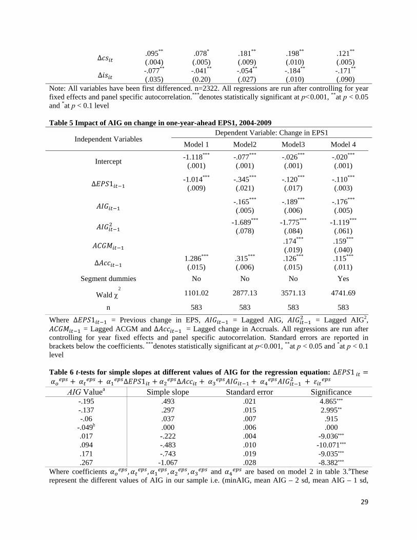
29  

∆ .095**

(.004) .078*

(.005) .181**

(.009) .198**

(.010) .121**

(.005)

∆ -.077**

(.035) -.041**

(0.20) -.054**

(.027) -.184**

(.010) -.171**

(.090) Note: All variables have been first differenced. n=2322. All regressions are run after controlling for year fixed effects and panel specific autocorrelation.***denotes statistically significant at p<0.001, **at p < 0.05 and *at p < 0.1 level Table 5 Impact of AIG on change in one-year-ahead EPS1, 2004-2009

Independent Variables Dependent Variable: Change in EPS1

Model 1 Model2 Model3 Model 4

Intercept -1.118***

(.001) -.077*** (.001)

-.026*** (.001)

-.020*** (.001)

∆ 1-1.014***

(.009) -.345*** (.021)

-.120*** (.017)

-.110*** (.003)

  -.165*** (.005)

-.189*** (.006)

-.176*** (.005)

  -1.689***

(.078) -1.775***

(.084) -1.119***

(.061)

  .174***

(.019) .159*** (.040)

∆  1.286***

(.015) .315***

(.006) .126***

(.015) .115***

(.011)

Segment dummies No No No Yes

Wald 2

1101.02 2877.13 3571.13 4741.69

n 583 583 583 583

Where ∆ 1 = Previous change in EPS, = Lagged AIG, = Lagged AIG2,   = Lagged ACGM and ∆ = Lagged change in Accruals. All regressions are run after

controlling for year fixed effects and panel specific autocorrelation. Standard errors are reported in brackets below the coefficients. ***denotes statistically significant at p<0.001, **at p < 0.05 and *at p < 0.1 level Table 6 t-tests for simple slopes at different values of AIG for the regression equation: ∆ 1       ∆ 1 ∆    

  

AIG Valuea Simple slope Standard error Significance -.195 .493 .021 4.865*** -.137 .297 .015 2.995** -.06 .037 .007 .915

-.049b .000 .006 .000 .017 -.222 .004 -9.036*** .094 -.483 .010 -10.071*** .171 -.743 .019 -9.035*** .267 -1.067 .028 -8.382***

Where coefficients , , , , and are based on model 2 in table 3.aThese represent the different values of AIG in our sample i.e. (minAIG, mean AIG – 2 sd, mean AIG – 1 sd,

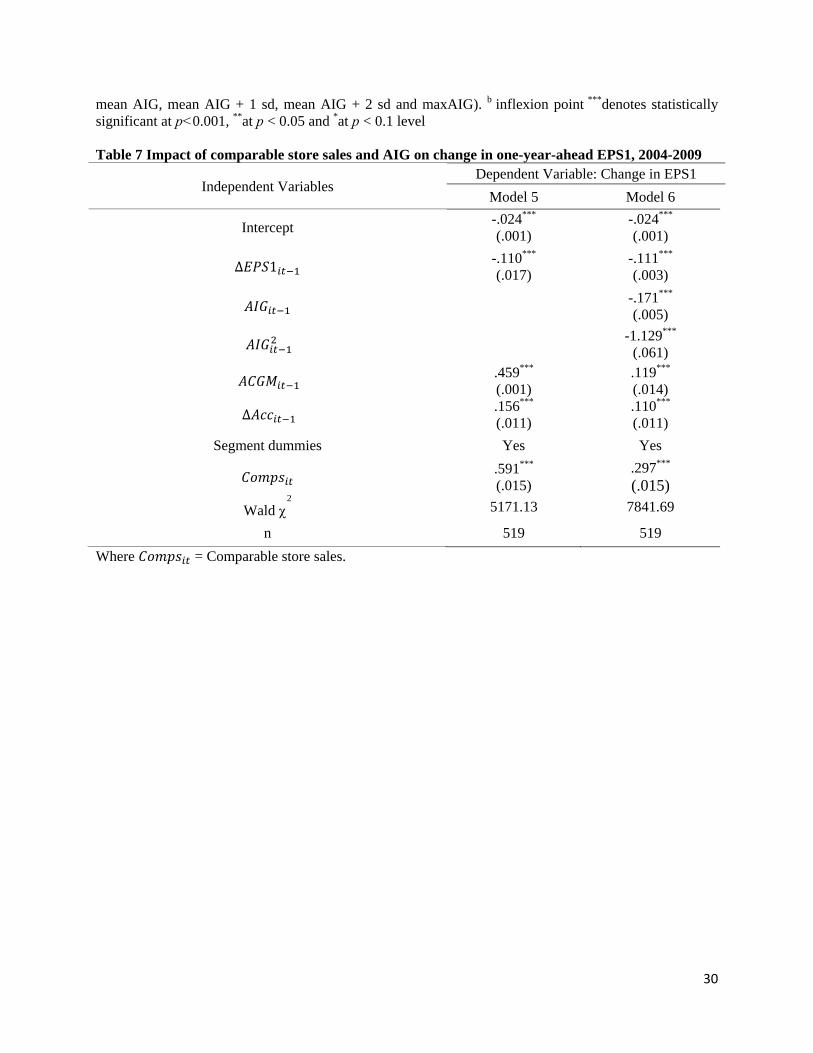
30  

mean AIG, mean AIG + 1 sd, mean AIG + 2 sd and maxAIG). b inflexion point ***denotes statistically significant at p<0.001, **at p < 0.05 and *at p < 0.1 level Table 7 Impact of comparable store sales and AIG on change in one-year-ahead EPS1, 2004-2009

Independent Variables Dependent Variable: Change in EPS1

Model 5 Model 6

Intercept -.024*** (.001)

-.024*** (.001)

∆ 1  -.110*** (.017)

-.111*** (.003)

  -.171*** (.005)

    -1.129***

(.061)

   .459*** (.001)

.119*** (.014)

 ∆  .156***

(.011) .110***

(.011)

Segment dummies Yes Yes

 .591*** (.015)

.297*** (.015)

Wald 2

5171.13 7841.69

n 519 519

Where = Comparable store sales.

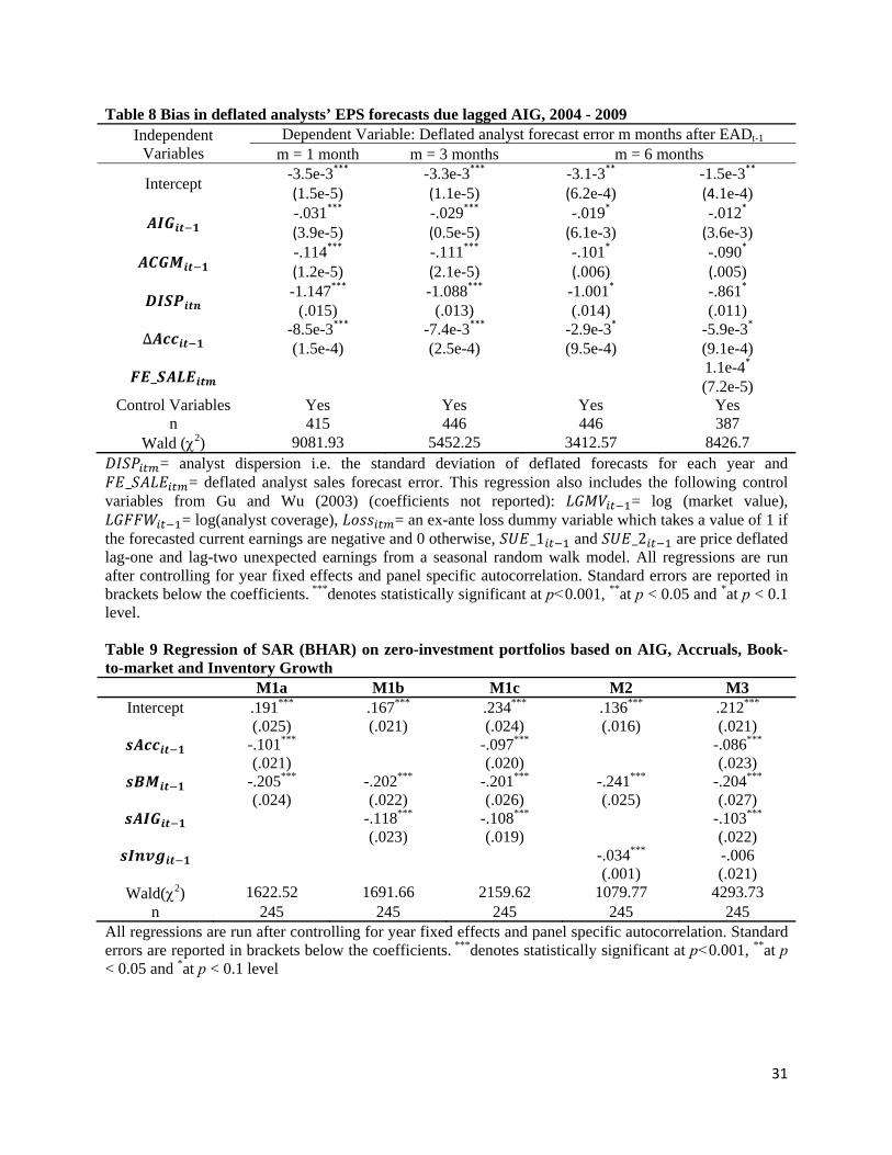
31  

Table 8 Bias in deflated analysts’ EPS forecasts due lagged AIG, 2004 - 2009

Independent Variables

Dependent Variable: Deflated analyst forecast error m months after EADt-1

m = 1 month m = 3 months m = 6 months

Intercept -3.5e-3*** 

(1.5e-5) -3.3e-3*** (1.1e-5)

-3.1-3** (6.2e-4)

-1.5e-3** (4.1e-4)

 -.031*** (3.9e-5)

-.029***

(0.5e-5) -.019*

(6.1e-3) -.012*

(3.6e-3)

 -.114*** (1.2e-5)

-.111***

(2.1e-5) -.101*

(.006) -.090*

(.005)

 -1.147*** 

(.015) -1.088***

(.013) -1.001*

(.014) -.861*

(.011)

∆  -8.5e-3*** 

(1.5e-4) -7.4e-3***

(2.5e-4) -2.9e-3*

(9.5e-4) -5.9e-3*

(9.1e-4)

_   1.1e-4* (7.2e-5)

Control Variables Yes Yes Yes Yes n 415 446 446 387

Wald (2) 9081.93 5452.25 3412.57 8426.7 = analyst dispersion i.e. the standard deviation of deflated forecasts for each year and

_ = deflated analyst sales forecast error. This regression also includes the following control variables from Gu and Wu (2003) (coefficients not reported): = log (market value),

= log(analyst coverage), = an ex-ante loss dummy variable which takes a value of 1 if the forecasted current earnings are negative and 0 otherwise, _1 and _2 are price deflated lag-one and lag-two unexpected earnings from a seasonal random walk model. All regressions are run after controlling for year fixed effects and panel specific autocorrelation. Standard errors are reported in brackets below the coefficients. ***denotes statistically significant at p<0.001, **at p < 0.05 and *at p < 0.1 level. Table 9 Regression of SAR (BHAR) on zero-investment portfolios based on AIG, Accruals, Book-to-market and Inventory Growth

M1a M1b M1c M2 M3 Intercept .191***

(.025) .167***

(.021) .234***

(.024) .136***

(.016) .212***

(.021)   -.101***

(.021) -.097***

(.020) -.086***

(.023)   -.205***

(.024) -.202***

(.022) -.201***

(.026) -.241***

(.025) -.204***

(.027)   -.118***

(.023) -.108***

(.019) -.103***

(.022)   -.034***

(.001) -.006 (.021)

Wald(2) 1622.52 1691.66 2159.62 1079.77 4293.73 n 245 245 245 245 245

All regressions are run after controlling for year fixed effects and panel specific autocorrelation. Standard errors are reported in brackets below the coefficients. ***denotes statistically significant at p<0.001, **at p < 0.05 and *at p < 0.1 level

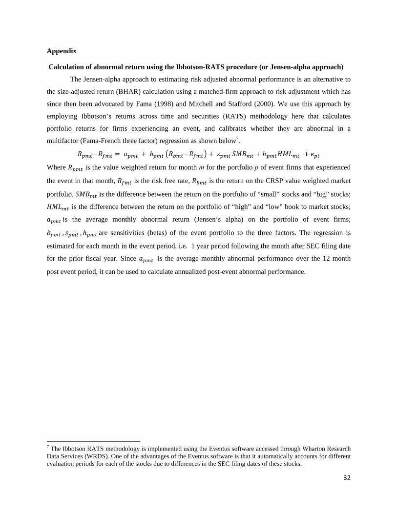
32  

Appendix

Calculation of abnormal return using the Ibbotson-RATS procedure (or Jensen-alpha approach)

The Jensen-alpha approach to estimating risk adjusted abnormal performance is an alternative to

the size-adjusted return (BHAR) calculation using a matched-firm approach to risk adjustment which has

since then been advocated by Fama (1998) and Mitchell and Stafford (2000). We use this approach by

employing Ibbotson’s returns across time and securities (RATS) methodology here that calculates

portfolio returns for firms experiencing an event, and calibrates whether they are abnormal in a

multifactor (Fama-French three factor) regression as shown below7.

              

Where is the value weighted return for month m for the portfolio p of event firms that experienced

the event in that month, is the risk free rate, is the return on the CRSP value weighted market

portfolio, is the difference between the return on the portfolio of “small” stocks and “big” stocks;

  is the difference between the return on the portfolio of “high” and “low” book to market stocks;

 is the average monthly abnormal return (Jensen’s alpha) on the portfolio of event firms;

 ,  ,  are sensitivities (betas) of the event portfolio to the three factors. The regression is

estimated for each month in the event period, i.e. 1 year period following the month after SEC filing date

for the prior fiscal year. Since   is the average monthly abnormal performance over the 12 month

post event period, it can be used to calculate annualized post-event abnormal performance.  

                                                            7 The Ibbotson RATS methodology is implemented using the Eventus software accessed through Wharton Research Data Services (WRDS). One of the advantages of the Eventus software is that it automatically accounts for different evaluation periods for each of the stocks due to differences in the SEC filing dates of these stocks.