the relationship between corruption and income inequality

THE RELATIONSHIP BETWEEN CORRUPTION AND INCOME INEQUALITY: A CROSS-

NATIONAL STUDY

A Thesis

submitted to the Faculty of the

Graduate School of Arts and Sciences of Georgetown University

in partial fulfillment of the requirements for the

degree of

Master of Public Policy

in Public Policy

By

Michael A. Mehen, M.A.

Washington, DC

April 19, 2013

ii

Copyright 2013 by Michael A. Mehen

All Rights Reserved

iii

THE RELATIONSHIP BETWEEN CORRUPTION AND INCOME INEQUALITY: A CROSS-

NATIONAL STUDY

Michael A. Mehen, M.A.

Thesis Advisor: Robert W. Bednarzik, Ph.D.

ABSTRACT

This paper analyzes the relationship between income inequality levels and corruption

levels. The hypothesis of the paper is that income inequality levels are positively correlated with

corruption levels, and is based upon theoretical arguments on incentive structures specific to

high-inequality societies. The paper proposes OLS estimation and 2SLS regression models for

data analysis, using Transparency International’s Corruptions Perceptions Index and the World

Bank’s Control of Corruption Index as measures of corruption, Gini coefficients as measures of

income inequality, and includes additional economic, political and cultural factors. Regression

analysis results on the sample of 126 countries support the hypothesis of a positive correlation

between income inequality and corruption. The results suggest that redistributive measures to

mitigate income inequality may curb the negative economic effects of corruption.

iv

The research and writing of this thesis

is dedicated to everyone who helped along the way.

Many thanks,

Michael A. Mehen

v

TABLE OF CONTENTS

Introduction ..........................................................................................................................1

Literature Review.................................................................................................................2

Hypothesis, Methodology and Data Sources .......................................................................9

Analysis..............................................................................................................................24

Policy Implications ............................................................................................................33

Appendix 1: Pairwise correlations between primary independent variables .....................36

Appendix 2: Results of Diagnostic Tests ...........................................................................37

References ..........................................................................................................................38

1

Introduction

The costs of corruption, or the misuse of public office for private gain, are widespread

and relatively similar across countries: corruption is associated with lower economic growth and

foreign investment, diminished government legitimacy, the destabilization of democratic

institutions and distortions in public spending. The World Bank has estimated that a total of $1

trillion dollars are paid in bribes annually, worldwide. That figure does not include the extent of

public funds that are embezzled or the theft of public assets, for which estimates remain difficult.

Moreover, the UN Economic and Social Council estimates that corruption prevents 30 percent of

all development assistance from reaching its targeted destination.

Yet the reasons why corruption tends to be more rampant in some countries than others

remain a source of debate. Cross-national variation in corruption has been the subject of

increasing empirical research, largely owing to the development of indices of corruption for

various countries that have sought to measure an inherently elusive phenomenon. The most

commonly used indices are Transparency International’s Corruption Perceptions Index (CPI),

and the World Bank’s Control of Corruption Index (CCI), each of which compile information

from a number of sources, primarily survey data from investment consultants, international and

domestic businesspeople, and expert panels on levels of perceived corruption. Despite the

limitations of perception-based indices, research has yielded robust evidence of some patterns in

cross-national variance that could be of potential use in designing and adapting anti-corruption

initiatives and reforms to different national contexts.

The present paper employs data from perception-based indices on corruption to examine

the relationship between income inequality and corruption. Income inequality has received

relatively little attention from corruption researchers, though the studies that have been done

show strong evidence of its association with corruption, albeit through different channels.

2

Moreover, existing studies rely on somewhat older data and exclude important factors cited in

other studies on cross-national variation in corruption. By further examining the link between

income inequality and corruption, a better understanding can be reached on whether this

particular issue could be a target for reform, or, if intractable, a factor to be considered in

devising anti-corruption strategies in countries with high degrees of inequality. Given the

complexity of corruption, an extensive set of factors must be considered to tease out the effects

of any single variable. The present paper’s aim is to devise a more rigorous analytical model to

further isolate and identify income inequality’s relationship to corruption, as well as to employ

more current data. In order to better account for this context it is useful to review broader, more

general analyses of corruption that have yielded evidence on various factors before moving on to

literature on the specific influence of income inequality.

Literature Review

An extensive amount of literature has been devoted to corruption, with much of the

earlier work having a more theoretical or qualitative basis. The recent development of corruption

perception measures, however, has led to the rapid growth over the last two decades of

quantitative, empirical research into the factors behind corruption, which is the focus of the

present paper.

Two surveys of literature on cross-national empirical research on corruption provide

background on the prevailing consensus in the field. Lambsdorff (2005) lists several areas where

evidence has been found for the correlation of specific factors with corruption: 1) regulatory

quality - specifically the number of procedures, time and official cost of opening a business,

(Djankov, et al. 2002) the vagueness and laxness of government regulation (Lambsdorff and

Cornelius, 2000), and highly diversified tariff rates (Gatti, 1999); 2) lack of economic

3

competition - ineffective or non-existent antitrust laws (Ades and DiTella, 1996) and lack of

integration into the global economy (Sandholtz and Gray, 2003); 3) government structure, where

democratic regimes (though specifically those where democracy has been present for decades)

were associated with less corruption than autocratic or authoritarian regimes (Montinola and

Jackmann, 2002); and 4) forms of democracy, where parliamentary systems were associated with

less corruption than presidential systems.

Treisman (2007) in his survey builds upon Lambsdorff by noting that “the strongest and

most consistent finding of the new empirical work was that lower perceived corruption correlates

closely with higher economic development,” (p. 223) though the channels by which it does so is

still a matter of debate. Treisman also outlines evidence that has emerged of correlations between

levels of corruption and economies oriented toward natural resources, especially for exports,

which are hypothesized to offer more avenues for bureaucrats to extract corrupt fees (Ades and

Di Tella, 1999). It should also be noted that the author describes having failed to find significant

linkages between corruption perceptions and income inequality (p. 239).

In addition to economic and governmental factors, country-specific culture and values

variables have also yielded evidence of being possible influences on disparities in corruption

levels across countries. Lambsdorff (2005) outlines research that has shown levels of trust and

acceptance of hierarchy (La Porta et al., 1997) were positively and negatively correlated with

levels of corruption, respectively. Other variables that have been examined include secular-

rational attitudes towards authority as opposed to particularistic or family loyalty, where the

former is correlated with less corruption (Sandholtz and Taagepera, 2005); and “generalized

trust,” or the belief that favors will be reciprocated (Lambsdorff and Cornelius, 2000).

4

Among the first and most seminal papers examining cross-national influences on

corruption was Treisman (2000), which examined the relationships of various economic,

cultural, legal and religious factors with levels of perceived corruption. The model’s dependent

variable was the CPI from 1996, 1997 and 1998. The results showed significantly lower levels of

corruption among: (1) countries with a British colonial heritage, which the author hypothesized

arose from common law traditions based on protecting private property from state encroachment;

(2) countries with higher portions of Protestants in their populations, hypothesized to arise from

“greater tolerance for challenges to authority and for individual dissent, even when threatening to

social hierarchies,” (p. 427); (3) countries where raw materials constitute a smaller share of

exports; (4) countries with higher GDP per capita; (5) non-federalist states (i.e., more

centralized states); (6) countries that have had continued democracy since 1950; and (7)

countries with greater openness to trade. While the author left the interplay between cultural and

economic factors to be explored in the future, the paper managed to identify a set of cultural and

religious variables that henceforth would be routinely used in identifying other factors correlated

with corruption.

Another possible influence on corruption is national levels of accountability and

transparency, typically enhanced through an active and independent media and laws governing

the financial transparency of political actors.

Brunetti and Weder (2001) examine the relationship between press freedom and

corruption levels. The authors use an OLS estimation model, with corruption measured by the

International Country Risk Guide (ICRG), which is based on subjective analysis of political,

financial and economic data, and press freedom as measured by Freedom House. Their model

includes additional variables for institutional quality, bureaucratic quality, GDP per capita,

5

human capital, trade openness and ethno-linguistic diversity. The authors find a statistically

significant negative association between press freedom and independence and corruption levels.

Djankov et al. (2009) build upon studies addressing the relationship press freedom and

corruption levels by examining an additional factor affecting the transparency and accountability

of the public sector: national laws requiring that politicians disclose personal financial

information, in particular assets, gifts and possible conflicts of interest. Using an OLS estimation

model, with corruption measured by the ICRG, and including variables for democracy as

measured by Freedom House, a proportional representation electoral system and press freedom,

the authors find a statistically significant negative association between the existence of national

public disclosure laws for politicians and levels of corruption.

Two articles have dealt specifically with the relationship between income inequality and

corruption. Gupta et al. (2002) examined the relationship of corruption to income inequality by

positing a series of channels. First, corruption could be correlated with income inequality due to

diminished poverty reduction from a general attenuation of economic growth. Second, corruption

could be correlated with skewed tax collection and administration that disproportionately favors

wealthy groups. Third, corruption on the part of wealthy segments of the society could lead to

the capture of funds through the creation of programs in their own favor, or through the

siphoning of funds from taxes or duties, with each case correlated with income inequality.

Fourth, the costs of corruption could be correlated with diminished human capital formation

through lower education and health spending. Fifth, corruption creates generally higher risk

premiums on investments that would ultimately reinforce income inequality by making

investments by more marginal, less well-connected groups prohibitively expensive. The authors

use empirical models to test the effects of corruption on income inequality. Gini coefficients for

6

a cross-section of 37 countries are regressed on natural resource abundance, education inequality,

capital stock/GDP ratio, as well as other variables, and indices for corruption based on the CPI

for 1995-1997.1 The primary shortcomings of the paper, however, include: (1) its small sample

size, (2) the relatively dated data in terms of corruption perception indices, which have now

expanded in terms of their breadth of coverage and depth of survey information for each

country’s composite score, and (3) the use of a democracy measure indicating whether the

country had been democratic for the past 46 years, which precluded analysis of discrepancies

(which are considerable) in corruption perception scores among states relatively new to

democracy.

You and Khagram (2005) explored the possibility that the relationship between income

inequality and corruption was a vicious circle, whereby corruption further entrenches existing

income inequality. The authors base this theory upon a comparative analysis of 129 countries

using the CCI and CPI as measures of the dependent variable, corruption levels, with averaged

Gini coefficients for each country for each year between 1971 and 1996 as the measure of their

primary independent variable of income inequality. The authors tested for the association of

perceptions and norms on corruption for each country using the World Values Survey, and

control for GDP per capita, trade openness, natural resource abundance, democracy, federalism,

religion, legal origins and ethno-linguistic fractionalization.2 Their results show a substantive

negative association between income inequality and corruption perception index scores, as well

1 A second model used various instruments for corruption levels, including a democracy variable, as well as

ethnicity, latitude, initial levels of corruption and ratio of government spending to GDP. The regression using

instruments yields more substantive results than the OLS regression, with a one standard deviation worsening in the

country’s corruption index score associated with an increase of 11 points in the country’s Gini coefficient (where the

average Gini coefficient among the country sample is 39). 2 To address the issue of the direction of influence between the variables, the authors use “mature cohort size” as an

instrumental variable for inequality, i.e. the ratio of the population aged 40 to 56 to that of the population between

15 and 69 years old; and distance from the equator and the prevalence of malaria as instruments for economic

development.

7

as support for their hypothesis that income inequality has a stronger correlation with corruption

in more democratic societies, as corruption becomes the means of preserving inequality where

overt authoritarian oppression is impossible. The authors further explore this relationship

through an interaction term between the Gini coefficients and a political rights score derived

from the Freedom House index. The authors find a strong correlation between income inequality

and perceptions of the acceptability of bribe taking by regressing data from the World Values

Survey on country level data, with the primary independent variable being averaged Gini

coefficients. An additional regression confirms the findings of Gupta et al. (2002), namely that

corruption is significantly associated with income inequality. The authors interpret this as further

evidence of a circular relationship between income inequality, and a possible explanation of the

persistence of income inequality over time.

A more recent study by Andres and Ramlogan-Dobson (2011) used panel data from 19

Latin American countries between 1982 and 2002 and found a negative correlation between

corruption and income inequality. Their model regressed Gini coefficients for each country on

corruption as measured by the ICRG, as well as school enrollment rates, openness to trade,

distribution of land resources, inflation, privatization and GDP per capita. The authors explained

the negative correlation between corruption and income inequality based upon the relative

prominence of informal sectors in Latin American countries, which disproportionately provide

employment to the poorest segments of society. Where corruption is reduced, the reasoning runs,

the informal sector shrinks, resulting in fewer jobs and a shift in income distribution. The authors

also suggested that in the cases of the countries from their sample large-scale programs aimed at

improving the welfare of the poor may also be those most prone to corruption in the first place. It

8

should be noted that the ICRG has been disputed as a reliable measure of corruption, and its use

as such discouraged by the ICRG’s editor-in-chief (Lambsdorff, 2005, p. 4)

Another recent study by Dincer and Gunlap (2012) focuses on income inequality and

corruption in the United States and reports a positive correlation between the two. The authors

regressed Gini coefficients from 48 states between 1981 and 1997 on the number of government

officials in each state convicted of crimes related to corruption for the year, as well as

demographic variables, unionization, tax and unemployment rates, and the employment shares of

agriculture and manufacturing. The authors’ choice of measurement for corruption is unusual,

given that the figure could be claimed to reflect more political pressure, or the competence of

police and the judiciary than corruption itself (Treisman, 2007, p. 216). The authors justify their

choice by noting that the measurement is based on federal convictions and hence not dependent

on variations in law enforcement across states. A valid comparable measure, however, does not

exist for cross-national comparisons.

The present paper aims to expand upon research on income inequality as a factor in

corruption by employing more recent data from the CPI, which has undergone significant

changes to its methodology since 2002, when it was last used by You and Khagram (2005). It

also seeks to add several variables to the models used in previous studies. These variables

include the prevalence of civil society organizations, values from the Press Freedom index, and

several indicator variables concerning country-specific laws on political contributions. In

addition, two questions dealing with attitudes towards authority and income equality are taken

from the World Values Survey conducted between 1996 and 2008.

9

Hypothesis, Methodology and Data Sources

Hypothesis

The theoretical basis of the hypothesis of this paper is grounded in previous research

showing a positive correlation between income inequality and corruption levels (Gupta et al.

2002, You and Khagram, 2005). The argument for a positive correlation between income

inequality and corruption levels is based upon the following premises: 1) In highly unequal

societies, the rich or well-connected have greater resources to purchase influence illegally; 2)

With increased inequality in a society, more pressure will be exerted by the poor for

redistributive measures such as progressive taxation, leading to an added incentive for the rich or

well-connected to employ political corruption in order to combat such measures and preserve the

status quo; and 3) Given that high-inequality societies are more likely to insufficiently provide

basic public services to the poor, the poor in turn will also depend on forms of corruption, albeit

petty corruption, to secure these services.

Methodology

The model for corruption and income inequality is estimated using an OLS regression

adapted from previous empirical research on corruption, specifically that of Treisman (2000) and

You and Khagram (2005). In addition, following You and Khagram (2005), to address the issue

of measurement error that may arise based upon the subjective nature of perception surveys, the

variable “mature cohort size” relative to the adult population is used as an instrumental variable

for income inequality in a 2SLS regression. This variable represents the relative size of the

population ranging in age from 40 to 59 years of age to the population aged 15 to 69 years.

Higgins and Williamson (1999) show that the relative size of the population aged between 40 to

59 years is a powerful predictor of inequality.

10

In each of the previous models, as well as the present one, the dependent variable is

corruption level as measured by either Transparency International’s Corruption Perception

Index, or the World Bank Institute’s Control of Corruption Index. The primary independent

variable, income inequality, is measured by Gini coefficient values, following You and Khagram

(2005), Gupta et al. (2002), and Dobson and Andres (2010).

Based on the results of model specification tests, the natural logarithm form for averaged

Gini coefficient proved to be the best fit. In addition, both GDP per capita and trade openness, or

the percentage of imports plus exports over GDP, were used in the natural logarithm form, as in

previous models (Treisman, 2000, You and Khagram, 2005). Other variables that have been

employed in previous studies that are present in the model used in this study included percentage

of the population identifying as Protestant, an indicator variable for whether or not the country’s

legal code originated in socialist/communist laws, and democracy as measured by the 1996-2002

averaged Freedom House political rights score. As in You and Khagram (2005), a quadratic term

was used for the Freedom House political rights score.3

Three variables were also created to test whether 1) GDP per capita, 2) socialist legal

code origin and 3) democracy as measured by the averaged Freedom House political rights score,

had associations with perceived corruption levels that varied depending on averaged Gini

coefficient values. You and Khagram (2005) employed a similar variable for the Freedom House

political rights score, based on the hypothesis that in more authoritarian regimes elites may use

repression as a substitute for corruption, and hence income inequality would have less of a

relationship to corruption in less democratic countries. Because an analogous relationship may

3 A number of variables used in previous models, including measures of ethno-linguistic fractionalization, English

Common Law, French, German and Scandinavian legal code origins, and the percentages of the population

identifying as Catholic or Muslim were excluded from the model based upon their consistent lack of statistical

significance in preliminary regression results.

11

exist in low versus high income countries, the relationship between GDP per capita and

perceived corruption levels in terms of averaged Gini coefficients was also included. A similar

variable for socialist legal code origin was included based on the fact that countries of this

category frequently feature low levels of income inequality combined with high levels of

corruption.

A series of additional regression analyses were conducted as added robustness checks

and to examine the influence of other variables that have been cited in the literature as having

relationships to perceived corruption levels.

Civil society organization prevalence as measured by the number of civil society

organization per capita in a country, and press freedom as measured by each country’s Press

Freedom Index Score for 2002 were available for the entire sample of countries. Each of these

variables is hypothesized to have a negative association with perceived corruption levels based

on the literature (Brunetti and Weder, 2003, Grimes, 2008).

Two variables were also included concerning attitudinal/cultural variables. The first

measured attitudes toward authority through responses to a question on the desirability of having

a strong leader, ranked from 1 (“very good”) to 4 (“very bad”). The second measured attitudes

towards income distribution through responses ranging between 1 (“incomes should be made

more equal”) to 10 (“we need larger income differences as incentives for individual effort”).

Based on the literature, the positive attitudes toward authority and income inequality are

hypothesized to have a positive association with perceived corruption levels (Sandholtz and

Taagepera, 2005).

12

Preliminary regressions results showed no statistically significant relationship between

perceived levels of corruption and national laws requiring the public disclosure of politicians’

financial information, in contrast to the findings of Djankov et al. (2009). In order to examine a

complementary aspect of the transparency of financial influence over political actors, four

variables concerning each country’s laws on political contributions and transparency were used

instead. These included 1) bans on corporate donations to political parties, 2) ceilings on

contributions to political parties, 3) ceilings on raisings by political parties, and 4) requirements

for the disclosure of contributions to political parties.

The model is as follows:

Y = β0+β1X1+β2X2 +β3X3+β4X4 +β5X5 +β6X6 +β7X7+ β8X8 + β9X9 + β10X10 +

+β11X11+β12X12 +β13X13+β14X14 +β15X15+ β16X16 + β17X17 + β18X18 + ε

Where:

Y = cpp/cci: Corruption level, measured by 1) Corruption Perceptions Index: 0 (most corrupt) to

10 (least corrupt) 2) Control of Corruption Index: -2.5 (most corrupt) to 2.5 (least corrupt) for

each country. Data from 2003-2010

X1 = ln gini: Income Inequality level, measured by the natural logarithm of averaged Gini

coefficient values for each country, ranging from 0 (least inequality) to 100 (most inequality).

Data from 1996-2002

X2 = lgdp: Economic development, measured by the natural logarithm of GDP per capita. Data

from 1996-2002

X3 = ltrade: trade openness, measured by the natural logarithm of percentage imports plus

exports over GDP. Data from 1996-2002.

X4 = natres: Natural resource abundance: measured by share of fuel, ore and metal exports from

total merchandise exports. Data from 1996-2002.

X5 = democ: Democracy: measured by the averaged Freedom House political rights score. Data

from 1996-2002

X6 = democsq: squared Democracy term, as measured by the averaged Freedom House political

rights score from 1996-2002.

X6 = soc_leg: indicator variable for whether the country’s legal code originated in

Socialist/Communist laws.

13

X7 =prot: Percentage of population identifying as Protestant Christians.

X8=soc_leg*gini: Variable for whether the country’s socialist legal code origin has a varying

association with corruption depending on averaged Gini coefficient value.

X9 =democ*gini: Variable for whether the country’s averaged Freedom House political rights

score has a varying association with corruption depending on averaged Gini coefficient value.

X10 =GDPperCap*gini: Variable for whether the country’s averaged GDP per capita has a

varying association with corruption depending on averaged Gini coefficient value.

X11 = cso_prev: civil society organization prevalence as measured by the number of civil society

organizations per capita from 2002.

X12 = press_free: Press Freedom Index score from 2002.

X13 =ban_corp: indicator variable for whether a country bans corporate donations to political

parties.

X14=ceil_cont: indicator variable for whether a country imposes ceilings on contributions to

political parties.

X 15=ceil_raise: indicator variable for whether a country imposes ceilings on raisings by political

parties.

X16 =disc_cont: indicator variable for whether a country requires public disclosure of

contributions to political parties.

X 17=WVS_auth: variable from the World Values Survey measuring responses to a question on

the desirability of having a strong leader, ranked from 1 (“very good”) to 4 (“very bad”).

X18 =WVS_income: variable from the World Values Survey measuring attitudes toward income

distribution ranging between 1 (“incomes should be made more equal”) to 10 (“we need larger

income differences as incentives for individual effort”).

ε = unexplained variance, error term

β0 = Y-intercept

β0, β1, β2, β3, β4, β5, β6, β7, β8, β9, β10, β11, β12, β13, β14, β15, β16, β17, β18 = coefficients of

respective independent variables

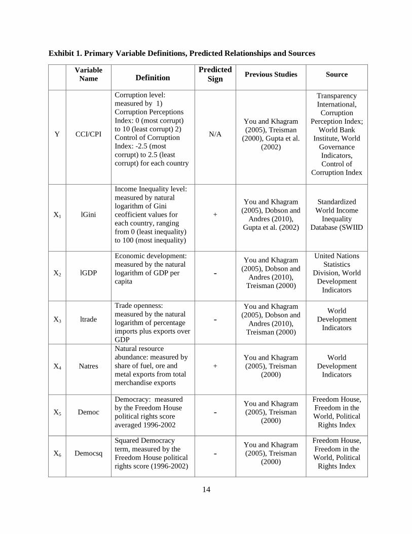
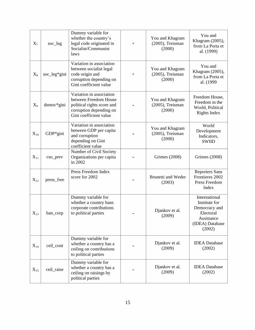
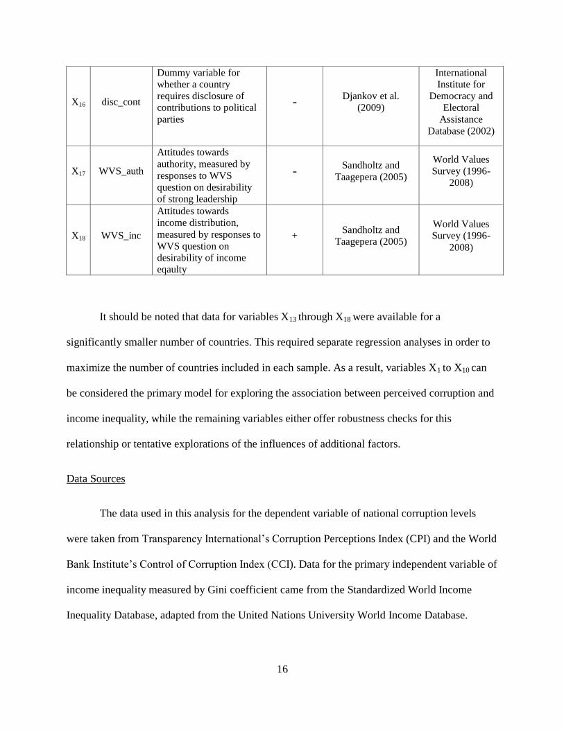
Exhibit 1 below defines these variables in greater detail, and presents the predicted

relationship between each of the independent variables and the dependent variable. The

theoretical basis for the predicted relationship is cited in the column listing previous studies.

14

Exhibit 1. Primary Variable Definitions, Predicted Relationships and Sources

Variable

Name Definition Predicted

Sign Previous Studies Source

Y CCI/CPI

Corruption level:

measured by 1)

Corruption Perceptions

Index: 0 (most corrupt)

to 10 (least corrupt) 2)

Control of Corruption

Index: -2.5 (most

corrupt) to 2.5 (least

corrupt) for each country

N/A

You and Khagram

(2005), Treisman

(2000), Gupta et al.

(2002)

Transparency

International,

Corruption

Perception Index;

World Bank

Institute, World

Governance

Indicators,

Control of

Corruption Index

X1 lGini

Income Inequality level:

measured by natural

logarithm of Gini

ceofficient values for

each country, ranging

from 0 (least inequality)

to 100 (most inequality)

+

You and Khagram

(2005), Dobson and

Andres (2010),

Gupta et al. (2002)

Standardized

World Income

Inequality

Database (SWIID

X2 lGDP

Economic development:

measured by the natural

logarithm of GDP per

capita -

You and Khagram

(2005), Dobson and

Andres (2010),

Treisman (2000)

United Nations

Statistics

Division, World

Development

Indicators

X3 ltrade

Trade openness:

measured by the natural

logarithm of percentage

imports plus exports over

GDP

-

You and Khagram

(2005), Dobson and

Andres (2010),

Treisman (2000)

World

Development

Indicators

X4 Natres

Natural resource

abundance: measured by

share of fuel, ore and

metal exports from total

merchandise exports

+

You and Khagram

(2005), Treisman

(2000)

World

Development

Indicators

X5 Democ

Democracy: measured

by the Freedom House

political rights score

averaged 1996-2002

- You and Khagram

(2005), Treisman

(2000)

Freedom House,

Freedom in the

World, Political

Rights Index

X6 Democsq

Squared Democracy

term, measured by the

Freedom House political

rights score (1996-2002)

- You and Khagram

(2005), Treisman

(2000)

Freedom House,

Freedom in the

World, Political

Rights Index

15

X7 soc_leg

Dummy variable for

whether the country’s

legal code originated in

Socialist/Communist

laws

+

You and Khagram

(2005), Treisman

(2000)

You and

Khagram (2005),

from La Porta et

al. (1999)

X8 soc_leg*gini

Variation in association

between socialist legal

code origin and

corruption depending on

Gini coefficient value

+

You and Khagram

(2005), Treisman

(2000)

You and

Khagram (2005),

from La Porta et

al. (1999

X9 democ*gini


between Freedom House

political rights score and

corruption depending on

Gini coefficient value

- You and Khagram

(2005), Treisman

(2000)

Freedom House,

Freedom in the

World, Political

Rights Index

X10 GDP*gini


between GDP per capita

and corruption

depending on Gini

coefficient value

- You and Khagram

(2005), Treisman

(2000)

World

Development

Indicators,

SWIID

X11 cso_prev

Number of Civil Society

Organizations per capita

in 2002 - Grimes (2008) Grimes (2008)

X12 press_free

Press Freedom Index

score for 2002 -

Brunetti and Weder

(2003)

Reporters Sans

Frontieres 2002

Press Freedom

Index

X13 ban_corp

Dummy variable for

whether a country bans

corporate contributions

to political parties - Djankov et al.

(2009)

International

Institute for

Democracy and

Electoral

Assistance

(IDEA) Database

(2002)

X14 ceil_cont

Dummy variable for

whether a country has a

ceiling on contributions

to political parties

- Djankov et al.

(2009)

IDEA Database

(2002)

X15 ceil_raise

Dummy variable for

whether a country has a

ceiling on raisings by

political parties

- Djankov et al.

(2009)

IDEA Database

(2002)

16

X16 disc_cont

Dummy variable for

whether a country

requires disclosure of

contributions to political

parties

- Djankov et al.

(2009)

International

Institute for

Democracy and

Electoral

Assistance

Database (2002)

X17 WVS_auth

Attitudes towards

authority, measured by

responses to WVS

question on desirability

of strong leadership

- Sandholtz and

Taagepera (2005)

World Values

Survey (1996-

2008)

X18 WVS_inc

Attitudes towards

income distribution,

measured by responses to

WVS question on

desirability of income

eqaulty

+ Sandholtz and

Taagepera (2005)

World Values

Survey (1996-

2008)

It should be noted that data for variables X13 through X18 were available for a

significantly smaller number of countries. This required separate regression analyses in order to

maximize the number of countries included in each sample. As a result, variables X1 to X10 can

be considered the primary model for exploring the association between perceived corruption and

income inequality, while the remaining variables either offer robustness checks for this

relationship or tentative explorations of the influences of additional factors.

Data Sources

The data used in this analysis for the dependent variable of national corruption levels

were taken from Transparency International’s Corruption Perceptions Index (CPI) and the World

Bank Institute’s Control of Corruption Index (CCI). Data for the primary independent variable of

income inequality measured by Gini coefficient came from the Standardized World Income

Inequality Database, adapted from the United Nations University World Income Database.

17

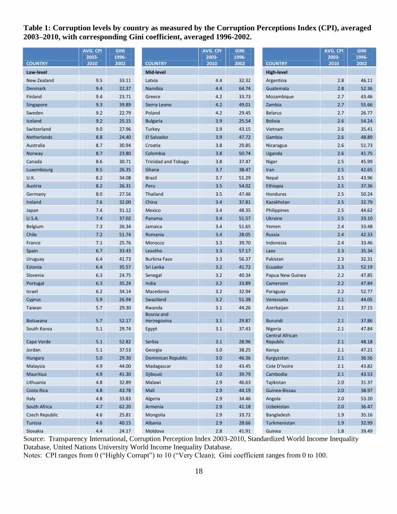
The CPI and CCI are based on survey data reflecting the opinions of international

business people, country experts and country inhabitants on perceived levels of corruption. The

CPI ranges from 0 (most corrupt) to 10 (least corrupt), while the CCI is a standardized score

ranging from -2.5 (most corrupt) to 2.5 (least corrupt), with a mean of zero and a standard

deviation of one. The Gini coefficient ranges from 0 to 100, with Gini of 0 signifying perfect

equality and a Gini of 100 signifying that a sole individual or household possesses the entirety of

the country’s income. Data from the CPI and CCI were taken from 2003-2010 and averaged,

while the Gini coefficients for each country were averaged from 1996-2002. A total of 126

countries comprise the sample used in this analysis.

Table 1 below presents data on corruption levels for each country in the present sample

measured by the CPI in descending order, as well as each country’s corresponding averaged Gini

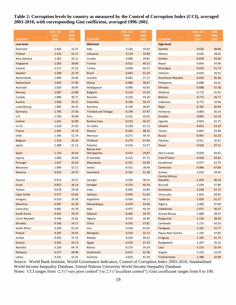
coefficient. Table 2, which follows, presents data on corruption levels for every country in the

present sample measured by the CCI in descending order, as well as each country’s

corresponding averaged Gini coefficient. In each table the averaged corruption score is listed in

the middle column, while the averaged Gini coefficient is listed in the right column.

18

Table 1: Corruption levels by country as measured by the Corruption Perceptions Index (CPI), averaged

2003–2010, with corresponding Gini coefficient, averaged 1996-2002.

COUNTRY

AVG. CPI 2003-2010

GINI 1996-2002

COUNTRY

AVG. CPI 2003-2010

GINI 1996-2002

COUNTRY

AVG. CPI 2003-2010

GINI 1996-2002

Low-level

Mid-level

High-level

New Zealand 9.5 33.11

Latvia 4.4 32.32

Argentina 2.8 46.11

Denmark 9.4 22.37

Namibia 4.4 64.74

Guatemala 2.8 52.36

Finland 9.4 23.71

Greece 4.2 33.73

Mozambique 2.7 43.46

Singapore 9.3 39.89

Sierra Leone 4.2 49.01

Zambia 2.7 55.66

Sweden 9.2 22.79

Poland 4.2 29.45

Belarus 2.7 26.77

Iceland 9.2 25.15

Bulgaria 3.9 25.54

Bolivia 2.6 54.24

Switzerland 9.0 27.96

Turkey 3.9 43.15

Vietnam 2.6 35.41

Netherlands 8.8 24.40

El Salvador 3.9 47.72

Gambia 2.6 48.89

Australia 8.7 30.94

Croatia 3.8 29.85

Nicaragua 2.6 51.73

Norway 8.7 23.80

Colombia 3.8 50.74

Uganda 2.6 41.75

Canada 8.6 30.71

Trinidad and Tobago 3.8 37.47

Niger 2.5 45.99

Luxembourg 8.5 26.35

Ghana 3.7 38.47

Iran 2.5 42.65

U.K. 8.2 34.08

Brazil 3.7 51.29

Nepal 2.5 43.96

Austria 8.2 26.31

Peru 3.5 54.02

Ethiopia 2.5 37.36

Germany 8.0 27.56

Thailand 3.5 47.46

Honduras 2.5 50.24

Ireland 7.6 32.00

China 3.4 37.81

Kazakhstan 2.5 32.79

Japan 7.4 31.12

Mexico 3.4 48.35

Philippines 2.5 44.62

U.S.A. 7.4 37.02

Panama 3.4 51.57

Ukraine 2.5 33.10

Belgium 7.3 26.34

Jamaica 3.4 51.65

Yemen 2.4 33.48

Chile 7.2 51.74

Romania 3.4 28.05

Russia 2.4 42.33

France 7.1 25.76

Morocco 3.3 39.70

Indonesia 2.4 33.46

Spain 6.7 33.43

Lesotho 3.3 57.17

Laos 2.3 35.34

Uruguay 6.4 41.73

Burkina Faso 3.3 56.37

Pakistan 2.3 32.31

Estonia 6.4 35.57

Sri Lanka 3.2 41.72

Ecuador 2.3 52.19

Slovenia 6.3 24.75

Senegal 3.2 40.34

Papua New Guinea 2.2 47.85

Portugal 6.3 35.24

India 3.2 33.89

Cameroon 2.2 47.84

Israel 6.2 34.14

Macedonia 3.2 32.94

Paraguay 2.2 52.77

Cyprus 5.9 26.94

Swaziland 3.2 51.38

Venezuela 2.1 44.05

Taiwan 5.7 29.30

Rwanda 3.1 44.26

Azerbaijan 2.1 37.15

Botswana 5.7 52.17

Bosnia and Herzegovina 3.1 29.87

Burundi 2.1 37.86

South Korea 5.1 29.74

Egypt 3.1 37.43

Nigeria 2.1 47.84

Cape Verde 5.1 52.82

Serbia 3.1 28.96

Central African Republic 2.1 48.18

Jordan 5.1 37.53

Georgia 3.0 38.25

Kenya 2.1 47.21

Hungary 5.0 29.30

Dominican Republic 3.0 46.36

Kyrgyzstan 2.1 36.56

Malaysia 4.9 44.00

Madagascar 3.0 43.45

Cote D'Ivoire 2.1 43.82

Mauritius 4.9 41.30

Djibouti 3.0 39.79

Cambodia 2.1 43.53

Lithuania 4.8 32.89

Malawi 2.9 46.63

Tajikistan 2.0 31.37

Costa Rica 4.8 43.78

Mali 2.9 44.19

Guinea-Bissau 2.0 38.97

Italy 4.8 33.83

Algeria 2.9 34.46

Angola 2.0 53.20

South Africa 4.7 62.20

Armenia 2.9 41.18

Uzbekistan 2.0 36.47

Czech Republic 4.6 25.81

Mongolia 2.9 33.72

Bangladesh 1.9 35.16

Tunisia 4.6 40.15

Albania 2.9 28.66

Turkmenistan 1.9 32.99

Slovakia 4.4 24.17

Moldova 2.8 41.91 Guinea 1.8 39.49

Source: Transparency International, Corruption Perception Index 2003-2010, Standardized World Income Inequality

Database, United Nations University World Income Inequality Database.

Notes: CPI ranges from 0 (“Highly Corrupt”) to 10 (“Very Clean); Gini coefficient ranges from 0 to 100.

19

Table 2: Corruption levels by country as measured by the Control of Corruption Index (CCI), averaged

2003-2010, with corresponding Gini coefficient, averaged 1996-2002.

COUNTRY

AVG. CCI 2003-2010

GINI 1996-2002

COUNTRY

AVG. CCI 2003-2010

GINI 1996-2002

COUNTRY

AVG. CCI 2003-2010

GINI 1996-2002

Low-level

Mid-level

High-level

Denmark 2.456 22.37

Italy 0.224 33.83

Gambia -0.626 48.89

Finland 2.410 23.71

Lithuania 0.178 32.89

Albania -0.630 28.66

New Zealand 2.365 33.11

Croatia 0.089 29.85

Zambia -0.639 55.66

Singapore 2.263 39.89

Tunisia -0.012 40.15

Nepal -0.643 43.96

Iceland 2.217 25.15

Turkey -0.030 43.15

Nicaragua -0.645 51.73

Sweden 2.208 22.79

Brazil -0.043 51.29

Vietnam -0.645 35.41

Netherlands 2.099 24.40

Lesotho -0.061 57.17

Dominican Republic -0.650 46.36

Switzerland 2.095 27.96

Ghana -0.086 38.47

Philippines -0.688 44.62

Australia 2.026 30.94

Madagascar -0.096 43.45

Ethiopia -0.688 37.36

Norway 2.007 23.80

Bulgaria -0.119 25.54

Moldova -0.719 41.91

Canada 1.980 30.71

Rwanda -0.163 44.26

Belarus -0.772 26.77

Austria 1.958 26.31

Colombia -0.196 50.74

Indonesia -0.775 33.46

Luxembourg 1.906 26.35

Romania -0.196 28.05

Niger -0.782 45.99

Germany 1.795 27.56

Trinidad and Tobago -0.199 37.47

Honduras -0.800 50.24

U.K. 1.769 34.08

Peru -0.252 54.02

Ecuador -0.805 52.19

Ireland 1.631 32.00

Burkina Faso -0.253 56.37

Uganda -0.810 41.75

U.S.A. 1.429 37.02

Sri Lanka -0.258 41.72

Ukraine -0.822 33.10

France 1.405 25.76

Mexico -0.264 48.35

Yemen -0.865 33.48

Chile 1.395 51.74

Morocco -0.271 39.70

Russia -0.907 42.33

Belgium 1.359 26.34

Thailand -0.279 47.46

Pakistan -0.921 32.31

Japan 1.288 31.12

Panama -0.310 51.57

Kenya -0.926 47.21

Spain 1.154 33.43

Bosnia and Herzegovina -0.314 29.87

Sierra Leone -0.929 49.01

Cyprus 1.060 26.94

El Salvador -0.315 47.72

Cote D'Ivoire -0.938 43.82

Portugal 1.037 35.24

Macedonia -0.325 32.94

Kazakhstan -0.977 32.79

Botswana 1.009 52.17

Serbia -0.331 28.96

Cameroon -0.984 47.84

Slovenia 0.935 24.75

Swaziland -0.332 51.38

Guinea -1.033 39.49

Estonia 0.913 35.57

Georgia -0.336 38.25

Central African Republic -1.034 48.18

Israel 0.852 34.14

Senegal -0.374 40.34

Burundi -1.034 37.86

Taiwan 0.678 29.30

India -0.405 33.89

Azerbaijan -1.038 37.15

Cape Verde 0.577 52.82

Jamaica -0.445 51.65

Venezuela -1.042 44.05

Hungary 0.519 29.30

Argentina -0.450 46.11

Tajikistan -1.059 31.37

Mauritius 0.497 41.30

Mozambique -0.470 43.46

Nigeria -1.069 47.84

Costa Rica 0.481 43.78

Mali -0.475 44.19

Uzbekistan -1.071 36.47

South Korea 0.452 29.74

Djibouti -0.485 39.79

Guinea-Bissau -1.088 38.97

Czech Republic 0.344 25.81

Algeria -0.534 34.46

Kyrgyzstan -1.118 36.56

Slovakia 0.336 24.17

China -0.535 37.81

Cambodia -1.137 43.53

South Africa 0.299 62.20

Iran -0.536 42.65

Paraguay -1.161 52.77

Poland 0.287 29.45

Mongolia -0.559 33.72

Papua New Guinea -1.195 47.85

Jordan 0.283 37.53

Malawi -0.564 46.63

Uruguay -1.195 41.73

Greece 0.242 33.73

Egypt -0.570 37.43

Bangladesh -1.207 35.16

Namibia 0.239 64.74

Bolivia -0.579 54.24

Laos -1.215 35.34

Malaysia 0.227 44.00

Guatemala -0.615 52.36

Angola -1.319 53.20

Latvia 0.225 32.32

Armenia -0.624 41.18

Turkmenistan -1.388 32.99

Source: World Bank Institute, World Governance Indicators, Control of Corruption Index 2003-2010, Standardized

World Income Inequality Database, United Nations University World Income Inequality Database.

Notes: CCI ranges from -2.5 (“very poor control”) to 2.5 (“excellent control”); Gini coefficient ranges from 0 to 100.

20

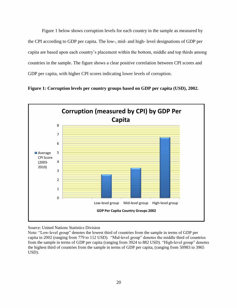
Figure 1 below shows corruption levels for each country in the sample as measured by

the CPI according to GDP per capita. The low-, mid- and high- level designations of GDP per

capita are based upon each country’s placement within the bottom, middle and top thirds among

countries in the sample. The figure shows a clear positive correlation between CPI scores and

GDP per capita, with higher CPI scores indicating lower levels of corruption.

Figure 1: Corruption levels per country groups based on GDP per capita (USD), 2002.

Source: United Nations Statistics Division

Note: “Low-level group” denotes the lowest third of countries from the sample in terms of GDP per

capita in 2002 (ranging from 779 to 112 USD). “Mid-level group” denotes the middle third of countries

from the sample in terms of GDP per capita (ranging from 3924 to 882 USD). “High-level group” denotes

the highest third of countries from the sample in terms of GDP per capita, (ranging from 50983 to 3965

USD).

0

1

2

3

4

5

6

7

8

Low-level group Mid-level group High-level group

GDP Per Capita Country Groups 2002

Corruption (measured by CPI) by GDP Per Capita

Average CPI Score (2003-2010)

21

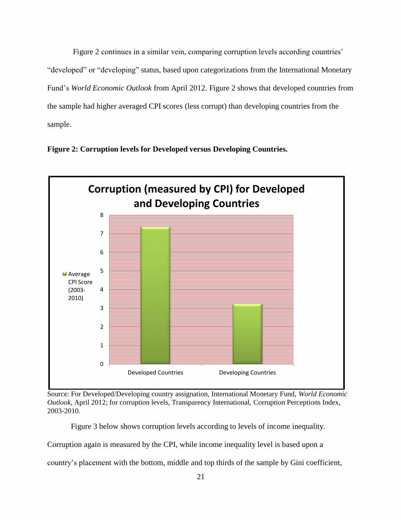
Figure 2 continues in a similar vein, comparing corruption levels according countries’

“developed” or “developing” status, based upon categorizations from the International Monetary

Fund’s World Economic Outlook from April 2012. Figure 2 shows that developed countries from

the sample had higher averaged CPI scores (less corrupt) than developing countries from the

sample.

Figure 2: Corruption levels for Developed versus Developing Countries.

Source: For Developed/Developing country assignation, International Monetary Fund, World Economic

Outlook, April 2012; for corruption levels, Transparency International, Corruption Perceptions Index,

2003-2010.

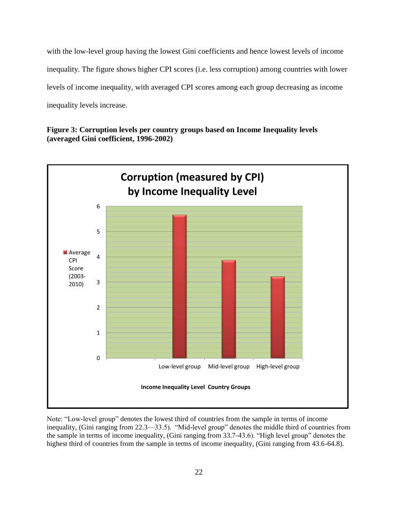
Figure 3 below shows corruption levels according to levels of income inequality.

Corruption again is measured by the CPI, while income inequality level is based upon a

country’s placement with the bottom, middle and top thirds of the sample by Gini coefficient,

0

1

2

3

4

5

6

7

8

Developed Countries Developing Countries

Corruption (measured by CPI) for Developed and Developing Countries


22

with the low-level group having the lowest Gini coefficients and hence lowest levels of income

inequality. The figure shows higher CPI scores (i.e. less corruption) among countries with lower

levels of income inequality, with averaged CPI scores among each group decreasing as income

inequality levels increase.

Figure 3: Corruption levels per country groups based on Income Inequality levels

(averaged Gini coefficient, 1996-2002)

Note: “Low-level group” denotes the lowest third of countries from the sample in terms of income

inequality, (Gini ranging from 22.3—33.5). “Mid-level group” denotes the middle third of countries from

the sample in terms of income inequality, (Gini ranging from 33.7-43.6). “High level group” denotes the

highest third of countries from the sample in terms of income inequality, (Gini ranging from 43.6-64.8).

0

1

2

3

4

5

6

Low-level group Mid-level group High-level group

Income Inequality Level Country Groups

Corruption (measured by CPI) by Income Inequality Level


23

Data on GDP per capita, natural resource abundance and trade openness were taken from

the World Bank’s World Development Indicator database, and used averaged data from 1996-

2002. Data for the democracy variable were taken from Freedom House’s Freedom in the World

Index, specifically each country’s political rights score averaged over the same period. Legal

code origin data was taken from La Porta et al. (1999).

For the supplementary variables, data for the press freedom variable were taken from the

Reporters Sans Frontieres 2002 Press Freedom Index. Data on the prevalence of civil society

organizations, as measured by the number of organizations per capita in each country, were taken

from Grimes (2008), and reflects rates from 2000. Attitudinal/cultural variable data were taken

from the World Values Survey (1996-2008). Data on the political contribution laws for each

country were taken from the International Institute for Democracy and Electoral Assistance

(IDEA), and represent a cross-section from 2002.4

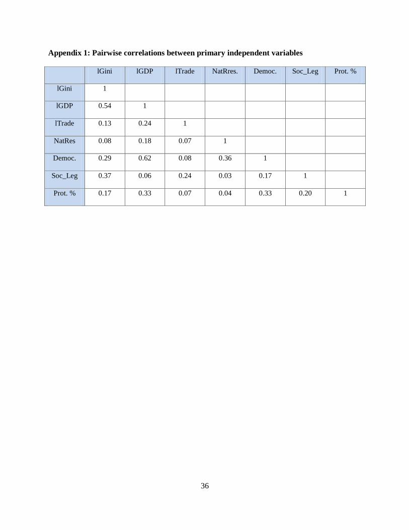
4 Appendix 1 presents pairwise correlations between the independent variables of the primary model, and indicates a

lack of multicollinearity.

24

Analysis

Three sets of regression analyses were performed. Each set supported the hypothesis of a

positive association between income inequality and corruption.5

The first set includes the largest sample of countries, and examines the relationship most

broadly, using a concise model including only control variables that in previous tests

demonstrated consistent significance. In addition, owing to the availability of data, four models

include variables related to sectors that are frequently the focus of anti-corruption campaigns: the

per capita number of civil society organizations and the Press Freedom index score for each

country from 2002. As a further robustness check, the first set of regression analyses included

three models using an instrumental variable for income inequality. Mature cohort size, or the

ratio of the population aged 40 to 59 years old relative to the population 15 to 69 years is

instrumented for the Gini coefficient, following You and Khagram (2005).

Table 3 presents the results of the first set of regression analyses using the largest sample.

Each of the six models explained more than 83 percent of the variation in corruption, indicating

strong predictive power in determining future levels of corruption.

In the three OLS estimations, the natural logarithm of the averaged 1996-2002 Gini

coefficient showed a statistically strong positive association with corruption levels as measured

by the averaged CPI from 2003-2010.6 In all three OLS estimations, the natural logarithm of the

averaged Gini coefficient was significant at the 1 percent level. In the three IV 2SLS regressions,

the natural logarithm of the averaged Gini coefficient (instrumented for with mature cohort size,

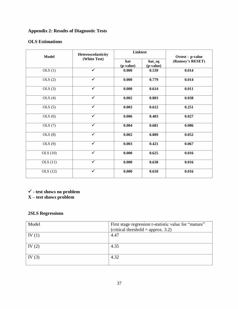
5Model diagnostics for all three sets of regression analyses are listed in Appendix 2.The results of the White test

showed no issues with heteroscedasticity. For the link test results, the “hat” p-value should be significant, and the

“hat squared,” or the coefficient of the squared linear predictor, should be insignificant, which was the case for all of

the models. The results of the Ramsey’s RESET test for omitted variables (“ovtest”) show no bias in this regard. For

the three 2SLS regressions, the first stage regression t-statistic value for “mature cohort size” was above the critical

threshold of 3.2. 6 The sign in the coefficient of the Gini is inverted because CPI scores range from 1 (most corrupt) to 10 (least

corrupt).

25

or “mature”) retained its statistically significant association with corruption levels, although to a

lesser degree at the 10 percent level. The six models strongly suggest the robustness of the

positive relationship between income inequality and corruption.

The natural logarithm of GDP per capita in all six models showed a strongly statistically

significant negative association with perceived corruption levels at the 1 percent level, as

expected from the literature (Treisman, 2000). Percentage of the country identifying as

Protestant also showed a very robust statistically significant negative association with perceived

corruption levels, a relationship that has also been revealed by previous studies (La Porta, et al.

1997).

Other variables that have been employed in previous cross-country empirical corruption

research included natural resource abundance, socialist legal code origins and democracy as

defined by Freedom House political rights score, showed statistically significant associations

with corruption to a slightly lesser extent, but with the expected signs. The use of a quadratic

term by You and Khagram (2005) for the Freedom House political rights score was reaffirmed in

all of the models.

Three variables were used to examine whether socialist legal code origin, Freedom House

index score and GDP per capita varied according to the natural logarithm of the averaged Gini

coefficient value. In contrast to You and Khagram (2005), who found that income inequality had

a stronger positive association with perceived corruption levels in countries with higher

democracy scores, this relationship was shown to be statistically significant only once, in OLS

(3), and in that instance at the 10 percent level. OLS (3) included Press Freedom Index score as

an additional independent variable, which may have contributed toward greater variation in the

democracy score.

26

At the same time, two variables previously unexplored in the literature showed

statistically significant associations with perceived corruption levels in multiple models. The

variable examining socialist legal code origin and Gini coefficients showed a statistically

significant positive association with perceived corruption levels in four of the six models at the

10 percent level, and in OLS(1) at the 5 percent level. Post-socialist or currently socialist legal

code countries frequently combine high levels of corruption with moderate to low levels of

income inequality. The results suggest that in these countries higher income inequality is still

associated with higher levels of corruption, and that the relationship intensifies as income

inequality increases.

The variable examining GDP per capita and Gini coefficients showed a statistically

significant positive association with perceived corruption levels in five of the six models,

including two, OLS(1) and OLS(2), where it was significant at the 5 percent level. The

relationship these results suggest is that the association between income inequality and

corruption is greater in higher-income countries. A possible explanation for why this might be

the case derives from the theoretical underpinnings of the relationship between corruption and

income inequality generally: corruption in highly unequal societies arises from effort by the rich

to preserve their status through corrupt practices at the expense of poorer segments of the

population (You and Khagram, 2005). This phenomenon may be more intense in higher income

countries where the lower segments of society may experience enough affluence to be politically

active or conscious, and hence more of a threat than in societies where the bottom rungs are

concerned more with basic subsistence.

The two variables tied to current strategies of anti-corruption campaigns, civil society

organization prevalence and the Press Freedom Index score, show no statistically significant

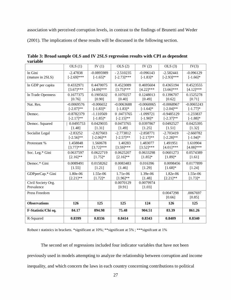
27

association with perceived corruption levels, in contrast to the findings of Brunetti and Weder

(2001). The implications of these results will be discussed in the following section.

Table 3: Broad sample OLS and IV 2SLS regression results with CPI as dependent

variable OLS (1) IV (1) OLS (2) IV (2) OLS (3) IV(3)

ln Gini

(mature in 2SLS)

-2.47838

[-2.69]***

-0.0895989

[-1.65]*

- 2.510235

[-2.73]***

-0.096143

[-1.83]*

-2.582441

[-2.93]***

-0.096129

[-1.66]*

ln GDP per capita 0.4332971

[3.67]***

0.4470075

[4.09]***

0.4523089

[3.75]***

0.4695604

[4.22]***

0.4365194

[3.66]***

0.4523555

[4.12]***

ln Trade Openness 0.1677375

[0.76]

0.1905632

[0.90]

0.1070257

[0.40]

0.1248013

[0.49]

0.1396707

[0.62]

0.1525278

[0.71]

Nat. Res. -0.0069576

[-2.07]**

-0.006652

[-1.83]*

-0.0063688

[-1.83]*

-0.0060065

[-1.64]*

-0.0068967

[-2.04]**

-0.0065243

[-1.77]*

Democ. -0.8782379

[-2.17]**

-1.110569

[-1.85]*

0 .0473765

[-2.15]**

-1.099721

[-1.90]*

-0.9485129

[-2.37]**

-1.233837

[-1.88]*

Democ. Squared | 0.0495753

[1.48]

0.0429035

[1.31]

0.0473765

[1.49]

0.0397867

[1.25]

0.0492527

[1.51]

0.0425395

[1.32]

Socialist Legal -2.83252

[-2.56]**

-2.827603

[-2.06]**

-2.773812

[-2.57]**

-2.858771

[-2.17]**

-2.703419

[-2.28]**

-2.660782

[-1.94]*

Protestant %

1.458848

[3.77]***

1.560678

[3.72]***

1.40283

[3.59]***

1.483077

[3.52]***

1.491951

[4.01]***

1.610904

[4.08]***

Soc. Leg.* Gini 0.0637597

[2.16]**

0.0622719

[1.75]*

0.0625207

[2.16]**

0.0633298

[1.85]*

0.0601273

[1.89]*

0.0574389

[1.61]

Democ.* Gini

0.0089491

[1.55]

0.0158262

[1.21]

0.0083483

[1.46]

0.016396

[1.29]

0.0098456

[1.68]*

0.0177899

[1.24]

GDPperCap.* Gini 1.80e-06

[2.21]**

1.55e-06

[1.72]*

1.71e-06

[1.96]**

1.39e-06

[1.48]

1.82e-06

[2.21]**

1.55e-06

[1.73]*

Civil Society Org.

Prevalence

0.0070129

[0.91]

0.0079974

[1.03]

Press Freedom 0.0047298

[0.66]

.0067697

[0.85]

Observations 126 125 125 124 126 125

F-Statistic/Chi sq. 84.17 894.98 75.48 904.51 83.39 861.26

R-Squared 0.8399 0.8336 0.8414 0.8343 0.8409 0.8340

Robust t statistics in brackets. *significant at 10%; **significant at 5% ; ***signifcant at 1%

The second set of regressions included four indicator variables that have not been

previously used in models attempting to analyze the relationship between corruption and income

inequality, and which concern the laws in each country concerning contributions to political

28

parties. CPI averaged between 2003-2010 was again used as the dependent variable. Owing to

missing data for these variables, the sample in this set of regression analyses is smaller than that

of the first.

Table 4 presents the results of the second set of regression analyses. Each of the six

models explained more than 84 percent of the variation in corruption, indicating a strong

predictive power in determining future levels of corruption.

OLS (4) shows that within this sample of countries the primary model employed in OLS

(1) still yields similar results, with averaged Gini coefficient, the log of GDP per capita, socialist

legal code origin and percentage of Protestants all significant at least at the 5 percent level.

Of the four variables introduced in this set of regression analyses, Ceiling on Raisings by

Parties was not statistically significant in any of the models in which it was included. Ceiling on

Contributions to Political Parties, which equals 1 if a ceiling exists on how much a donor can

contribute to political parties, showed a strongly statistically significant positive association with

perceived levels of corruption at the 1 percent level in both models in which it was included. Ban

on Corporate Donations to parties, which equals 1 if such a ban exists, also showed a positive

statistically significant association with perceived levels of corruption. When added to the

baseline model in OLS (6), it was statistically significant at the 5 percent level.

Disclosure of contributions to political parties, which equals 1 if provisions exist for such

disclosures, was not statistically significantly associated with perceived levels of corruption

when added to the primary model without the other political contribution law variables in OLS

(8). However, when these other variables are added, disclosure of contributions to parties showed

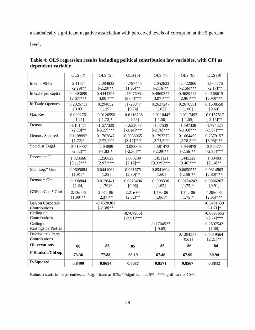
29

a statistically significant negative association with perceived levels of corruption at the 5 percent

level.

Table 4: OLS regression results including political contribution law variables, with CPI as

dependent variable

OLS (4) OLS (5) OLS (6) OLS (7) OLS (8) OLS (9)

ln Gini 96-02

-2.11371

[-2.29]**

-2.084833

[-2.29]**

-1.797456

[1.96]**

-2.052633

[-2.16]**

-2.422066

[-2.66]***

-1.865776

[-2.17]**


[2.67]***

0.4444293

[3.00]***

.4507693

[3.08]***

0.4860377

[3.07]***

0.4689443

[2.96]***

0.4168615

[2.90]***

ln Trade Openness 0.2326711

[0.83]

0.294852

[1.19]

.1728847

[0.74]

0.2637247

[1.02]

0.2676561

[1.00]

0.1508558

[0.69]

Nat. Res. -0.0092761

[-1.21]

-0.0126598

[-1.72]*

-0.0118708

[-1.55]

-0.0118442

[-1.50]

-0.0117493

[-1.55]

-0.0157517

[-2.15]**

Democ. -1.181471

[-2.00]**

-1.677329

[-3.27]***

-1.633677

[-3.14]***

-1.47539

[-2.76]***

-1.597338

[-3.03]***

-1.794625

[-3.67]***

Democ. Squared 0.1108992

[1.72]*

0.1762847

[2.77]***

0.2038065

[3.17]***

0.1793372

[2.74]***

0.1664469

[2.78]***

0.2379157

[3.95]***


[-2.32]**

-2.04889

[-1.83]*

-3.058895

[-2.36]**

-2.581472

[-2.09]**

-3.044978

[-2.56]**

-3.229774

[-2.93]***

Protestant % 1.323566

[3.11]***

1.250829

[2.97]***

1.000289

[2.12]**

1.451121

[3.339]***

1.445329

[3.46]***

1.00403

[2.14]**


[1.91]*

0.0441062

[1.38]

0.081675

[2.30]**

0.0541604

[1.60]

0.0650575

[-2.56]**

0.0814863

[2.60]***

Democ.* Gini

0.008804

[1.24]

0.0126441

[1.70]*

0.0073496

[0.96]

0 .008336

[1.05]

0 .0124243

[1.75]*

0.0066267

[0.91]


[1.99]**

2.07e-06

[2.37]**

2.21e-06

[2.52]**

1.79e-06

[1.86]*

1.74e-06

[1.75]*

1.98e-06

[2.65]***

Ban on Corporate

Contributions

-0.4520381

[-2.38]**

-0.3491639

[-1.71]*

Ceiling on

Contributions

-0.7079061

[-2.91]***

-0.8693655

[-2.74]***

Ceiling on

Raisings by Parties

-0.1704927

[-0.65]

0.2697542

[1.08]

Disclosure - Party

Contributions

0.1284557

[0.61]

0.5319564

[2.21]**

Observations 88 85 85 85 86 84

F-Statistic/Chi sq. 73.36 77.88 68.19 67.46 67.99 60.94

R-Squared 0.8499 0.8694 0.8687 0.8571 0.8567 0.8832

Robust t statistics in parentheses. *significant at 10%; **significant at 5% ; ***significant at 10%

30

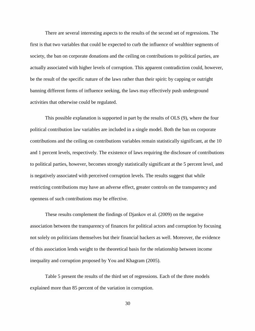
There are several interesting aspects to the results of the second set of regressions. The

first is that two variables that could be expected to curb the influence of wealthier segments of

society, the ban on corporate donations and the ceiling on contributions to political parties, are

actually associated with higher levels of corruption. This apparent contradiction could, however,

be the result of the specific nature of the laws rather than their spirit: by capping or outright

banning different forms of influence seeking, the laws may effectively push underground

activities that otherwise could be regulated.

This possible explanation is supported in part by the results of OLS (9), where the four

political contribution law variables are included in a single model. Both the ban on corporate

contributions and the ceiling on contributions variables remain statistically significant, at the 10

and 1 percent levels, respectively. The existence of laws requiring the disclosure of contributions

to political parties, however, becomes strongly statistically significant at the 5 percent level, and

is negatively associated with perceived corruption levels. The results suggest that while

restricting contributions may have an adverse effect, greater controls on the transparency and

openness of such contributions may be effective.

These results complement the findings of Djankov et al. (2009) on the negative

association between the transparency of finances for political actors and corruption by focusing

not solely on politicians themselves but their financial backers as well. Moreover, the evidence

of this association lends weight to the theoretical basis for the relationship between income

inequality and corruption proposed by You and Khagram (2005).

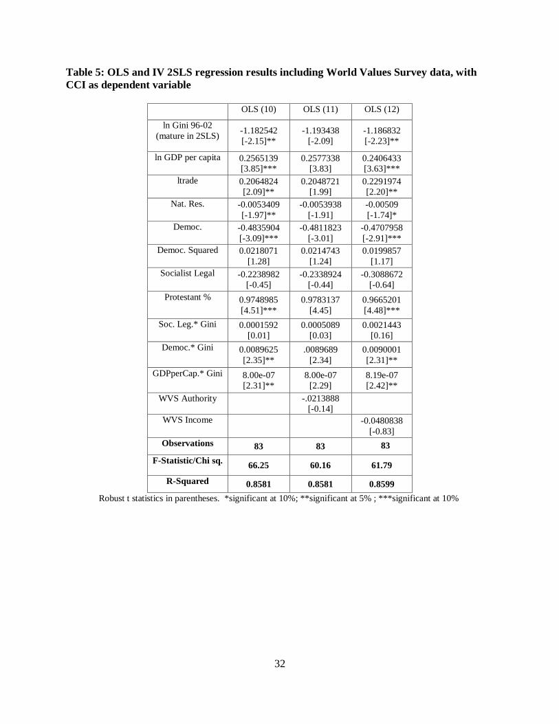
Table 5 present the results of the third set of regressions. Each of the three models

explained more than 85 percent of the variation in corruption.

31

The third set of regression analyses looked specifically at attitudinal and cultural

variables gleaned from the World Values Survey. Data on these variables included a smaller

sample of countries. The two variables included in the regression analyses concerned attitudes

toward authority (specifically, the desirability of having a “strong leader,” ranked on a scale of 1

to 4) and income distribution (whether incomes should be more (1) or less (10) equal).

Unfortunately, the first regression using the baseline model shown in OLS (1) with CPI

as the dependent variable failed to show a significant relationship between income inequality and

corruption.

Three models using a different measure of corruption, the World Bank Control of

Corruption Index (CCI), as the dependent variable were run using the data from the World

Values Survey. In all three models income inequality shows a strongly statistically significant

association with perceived corruption levels. The cultural/attitudinal variables, however, showed

no significant associations in the regressions in which they were included.

32

Table 5: OLS and IV 2SLS regression results including World Values Survey data, with

CCI as dependent variable

OLS (10) OLS (11) OLS (12)

ln Gini 96-02

(mature in 2SLS)

-1.182542

[-2.15]**

-1.193438

[-2.09]

-1.186832

[-2.23]**


[3.85]***

0.2577338

[3.83]

0.2406433

[3.63]***

ltrade 0.2064824

[2.09]**

0.2048721

[1.99]

0.2291974

[2.20]**

Nat. Res. -0.0053409

[-1.97]**

-0.0053938

[-1.91]

-0.00509

[-1.74]*

Democ. -0.4835904

[-3.09]***

-0.4811823

[-3.01]

-0.4707958

[-2.91]***

Democ. Squared 0.0218071

[1.28]

0.0214743

[1.24]

0.0199857

[1.17]


[-0.45]

-0.2338924

[-0.44]

-0.3088672

[-0.64]

Protestant % 0.9748985

[4.51]***

0.9783137

[4.45]

0.9665201

[4.48]***


[0.01]

0.0005089

[0.03]

0.0021443

[0.16]

Democ.* Gini

0.0089625

[2.35]**

.0089689

[2.34]

0.0090001

[2.31]**


[2.31]**

8.00e-07

[2.29]

8.19e-07

[2.42]**

WVS Authority

-.0213888

[-0.14]

WVS Income

-0.0480838

[-0.83]

Observations 83 83 83

F-Statistic/Chi sq. 66.25 60.16 61.79

R-Squared 0.8581 0.8581 0.8599

Robust t statistics in parentheses. *significant at 10%; **significant at 5% ; ***significant at 10%

33

Policy Implications

Corruption is a highly complex phenomenon that has been associated with a multitude of

economic, legal, cultural and demographic factors. Any anti-corruption campaign will fail if it

focuses on a single perceived cause at the expense of others. Moreover, much of the forms

corruption will take, and the pervasiveness with which it will manifest itself, are dependent on

country-specific conditions, making encompassing policy prescriptions for anti-corruption

efforts difficult and perhaps fundamentally misguided. However, by adding further evidence to

the relationship between income inequality and corruption this study may offer insight into how

certain forms of corruption may come about, as well as a possible explanation for why certain

factors previously thought to underlie corruption, and which have inspired anti-corruption

measures, have not been supported by empirical research. The results of this study also suggest

the possible long-term economic consequences of pronounced income inequality.

The main finding of this study was a robust positive association between income

inequality and corruption. The study used more recent data from the last decade, and built upon

the models of previous studies with a greater array of variables. The growing evidence of the

relationship between income inequality and corruption supports theories made by previous

research: in societies where a small economic elite emerges, the pressure to retain their status and

wealth may impel this elite to use their superior position to purchase influence, often illegally

(Khagram and You, 2005, Gupta et al., 2002).

The relationship also may provide an explanation for why previous studies of corruption

found higher levels of corruption associated with smaller government size, rather than vice versa

(Friedman, 2000, La Porta, 1999). Rather than a swollen public sector staffed by bribe-seeking

officials, corruption may in part arise from elites from the private sector aggressively attempting

34

to safeguard their interests. This would suggest that minimizing the public sector is not

necessarily the best basis for anti-corruption reform (You and Khagram, 2005).

Other measures frequently proposed to curb corruption have been the promotion of civil

society and media development (Brunetti and Weder, 2001). The results of this study found no

statistically significant association between either of these two factors and corruption level. This

should in no way suggest the downplaying of the importance of efforts in these areas. It may

nonetheless be the case that larger factors may play a part in corruption at the national level, and

that anti-corruption campaigns could profit from a greater diversity of emphases.

The failure to find significant statistical associations between cultural and attitudinal

variables taken from responses to the World Values Survey is tentatively encouraging. Given the

ingrained and largely irreversible nature of such factors, they are typically considered to lie

beyond the reach of conceivable reforms, and their possible lack of influence suggests measures

can be taken to combat corruption in countries where it is relatively entrenched (Lambsdorff,

2005).

The possible relationship between income inequality and corruption suggests that

measures to counteract the influence wielded by wealthy elites over the state could bring positive

results. One of the more salient avenues for this influence is in the form of financial

contributions and ties to political actors, and to political parties in particular. The results of this

study suggest that implementing greater regulation on the requisite degree of transparency and

openness of such ties may serve to curtail corruption, and perhaps to a greater extent that

comparable regulations on the kind or size of the contributions themselves.

Lastly, the study’s findings point to the possible long-term economic consequences of

income inequality. Keeping in mind the figures cited at the outset of this study on the sheer size

35

of the losses associated with corruption globally, over and above its harm to institutions and

political stability, any evidence that it may in part be associated with income inequality calls for

the possible consideration of redistributive measures. Whether such measures themselves have

associations with corruption levels, as suggested by Andres and Ramlogan-Dobson (2011),

should be investigated. In addition, other forms of inequality, including inequality in terms of

education, gender, ethnicity and political participation, could also be topics for further study.

36

Appendix 1: Pairwise correlations between primary independent variables

lGini lGDP lTrade NatRres. Democ. Soc_Leg Prot. %

lGini 1

lGDP 0.54 1

lTrade 0.13 0.24 1

NatRes 0.08 0.18 0.07 1

Democ. 0.29 0.62 0.08 0.36 1

Soc_Leg 0.37 0.06 0.24 0.03 0.17 1

Prot. % 0.17 0.33 0.07 0.04 0.33 0.20 1

37

Appendix 2: Results of Diagnostic Tests

OLS Estimations

Model Heteroscedasticity

(White Test)

Linktest

Ovtest – p-value

(Ramsey’s RESET) hat

(p-value)

hat_sq

(p-value)

OLS (1) 0.000 0.539 0.014

OLS (2) 0.000 0.779 0.014

OLS (3) 0.000 0.614 0.011

OLS (4) 0.002 0.803 0.038

OLS (5) 0.003 0.612 0.251

OLS (6) 0.006 0.403 0.027

OLS (7) 0.004 0.681 0.086

OLS (8) 0.002 0.809 0.052

OLS (9) 0.003 0.421 0.067

OLS (10) 0.000 0.625 0.016

OLS (11) 0.000 0.630 0.016

OLS (12) 0.000 0.618 0.016

- test shows no problem

X – test shows problem

2SLS Regressions

Model First stage regression t-statistic value for “mature”

(critical threshold = approx. 3.2)

IV (1) 4.47

IV (2) 4.35

IV (3) 4.32

38

References

Ades, A. and R. Di Tella (1996), ‘The causes and consequences of corruption: a review of

recent empirical contributions’, in B. Harris-White and G. White (eds), Liberalization and

the New Corruption, Institute of Development Studies Bulletin, Brighton, 27, 6–12.

Ades, A. and R. Di Tella (1999), ‘Rents, competition, and corruption’, American Economic

Review, 89, 982–94.

Andres, A.R. and C. Ramlogan-Dobson (2011), ‘Is corruption really bad for inequality?

Evidence from Latin America’, Journal of Development Studies, 47(7), 959-76

Becker, Gary S. 1995. “If you want to cut corruption, cut government.” Business Week 3454:26

Brunetti, Aymo, and Beatrice Weder. "A free press is bad news for corruption."Journal of Public

Economics 87.7 (2003): 1801-1824.

Dincer, O.C. and B. Gunalp (2012), ‘Corruption and income inequality in the United States’,

Contemporary Economic Policy, 30(2), 283-92

Djankov, S., R. La Porta, F. Lopez-de-Silanes and A. Shleifer (2002), ‘The regulation of

entry’, Quarterly Journal of Economics, 117(1), 1–37.

Djankov, Simeon, et al. “Disclosure by politicians.” No. w14703. National Bureau of Economic

Research, 2009.

Friedman, Eric, et al. "Dodging the grabbing hand: the determinants of unofficial activity in 69

countries." Journal of Public Economics 76.3 (2000): 459-493.

Gatti, R. (1999), ‘Corruption and trade tariffs, or a case for uniform tariffs’, World Bank

Policy Research Working Paper no. 2216.

Grimes, Marcia. "Contestation or complicity: Civil society as antidote or accessory to political

corruption." Paper presented at the 2008 Midwest Political Science Association, Chicago IL, 2-6

April 2008. (2008).)

Gupta, S., H. Davoodi and R. Alonso-Terme (2002), ‘Does corruption affect income inequality

and poverty?’, Economics of Governance, 3, 23–45.

Higgins, Matthew, and Jeffrey G. Williamson. “Explaining Inequality the World Round: Cohort

Size, Kuznets Curves, and Openness.” No. w7224. National Bureau of Economic Research,

1999.

Hofstede, G. (1997), Cultures and Organizations: Software of the Mind, New York: McGraw-

Hill.

39

Husted, B. (1999), ‘Wealth, culture, and corruption’, Journal of International Business Studies,

30(2), 339–60.

Lambsdorff, J. Graf and P. Cornelius (2000), ‘Corruption, foreign investment and growth’, in

K. Schwab, L. Cook, P. Cornelius, J.D. Sachs, S. Sievers and A. Warner (eds.), The Africa

Competitiveness Report 2000/2001, joint publication of the World Economic Forum and the

Institute for International Development, Harvard University, Oxford: Oxford University

Press, pp. 70–78.

Lambsdorff, J. Graf (2005), ‘Causes and consequences of corruption: What do we know from a

cross-section of countries?’, in Susan Rose-Ackerman (ed.), The International Handbook on the

Economics of Corruption, Northampton, 3-51

La Porta, R., F. Lopez-De-Silanes, A. Shleifer and R.W. Vishny (1997), ‘Trust in large

organisations’, American Economic Review, Papers and Proceedings, 137(2), 333–8.

Montinola, G. and R.W. Jackman (2002), ‘Sources of corruption: a cross-country study’,

British Journal of Political Science, 32, 147–70.

Sandholtz, W. and M. Gray (2003), ‘International integration and national corruption’,

International Organization, 57(4), 761–800.

Sandholtz,W. and R. Taagepera (2005), ‘Corruption, culture, and communism’, International

Review of Sociology, 15(1), 109–31.

Treisman, D. (2000), ‘The causes of corruption: a cross-national study’, Journal of Public

Economics, 76, 399–457.

Treisman, D. (2007), ‘What have we learned about the causes of corruption from years of cross-

national empirical research?’, Annual Review of Political Science, 10, 211-44

You, J.-S. and S. Khagram (2005), ‘Inequality and corruption’, American Sociological Review,

70(1), 136–57.

the relationship between corruption and income inequality

Documents