Cleared for Public Release

Distribution Unlimited

Sensor and Simulation Notes

Note 538

Idus Martiae 2009

The Relationship Between NEMP Standards and Simulator Performance Specifications

D. V. Giri Pro-Tech, 11-C Orchard Court, Alamo, CA 94507-1541

Dept. of Electrical and Computer Engineering, Univ. of New Mexico, Albuquerque, NM 87131

William D. Prather Air Force Research Laboratory/RDHP, Kirtland AFB, NM 87117

Carl E. Baum Dept. of Electrical and Computer Engineering, Univ. of New Mexico, Albuquerque, NM 87131

Abstract

There appears to be a general notion that a NEMP Standard can be used directly “as is” to specify the technical performance requirements for a simulator. However, a standard does not translate directly to a specification, and using a standard in this fashion can lead to technical as well as contractual problems. The objective of this note is to describe the difference between the two and to recommend ways to write a simulator performance specification in a way that is unambiguous and understandable by contractors and government personnel alike. The contribution from Mr. Prather was sponsored in part by the Defense Threat Reduction Agency (DTRA).

2

CONTENTS Section Page 1. Introduction………………………………………………………. 3 2. What is the NEMP Standard and where did it come from?........... 3 3. Review of Unclassified NEMP Standards……………………….. 6 4. Relationship between Standards and Specifications………………. 9 5. Proposed Format for Specifications………………………………. 12 Appendix A Examples of EMP Simulators……………………………………… 15

References………………………………………………………….. 19

3

1. Introduction. Quite often, persons tasked with writing the technical specifications for procuring a new NEMP simulator or upgrading an existing simulator, will simply require that the simulated environment conform to one of the NEMP standards instead of writing a suitable hardware specification. As we will discuss here, these are not the same thing, and using a standard for an acquisition can lead to technical as well as contractual problems. In this note, we will address the relationship between NEMP standards and NEMP specifications for procuring and assessing the performance of a simulator. In this, we are only concerned about the prompt-gamma or early time portion of the NEMP, typically called the E1 environment. There are several different civilian NEMP standards for this environment, and those are reviewed here. The classified military standards are of the same form, only the numbers are different, so the discussion herein applies to the military standards, also. 2. What is the NEMP Standard and where did it come from?

A NEMP standard is a model of the high altitude EMP environment that characterizes the NEMP threat. It is designed to characterize (or envelope) some number of nuclear weapon outputs. A standard is not a hardware specification. The specifications should be based on a standard, obviously, but simply citing a standard in hardware procurement is an incomplete way to specify the hardware, and this can lead to technical as well as legal problems. A complete specification of the electromagnetic environment to be simulated should describe both time-domain and frequency-domain quantities for the fields.

The standards are typically defined by an equation, expressed in time as well as frequency domain, often with accompanying plots.

The NEMP standard is defined in two ways: (a) a horizontally polarized, overhead incident plane wave (A plane wave has a free space impedance of Zo = E/H = 377�.) and (b) a vertically polarized, side-on incident plane wave. 2.1 Two Components of NEMP The HEMP has a vertical and horizontal (to the Earth’s surface) orientation that depends on the geomagnetic field orientation roughly below the burst (at an altitude of 30 km where the HEMP is “born”). A burst at the geomagnetic North Pole creates only a horizontal HEMP field in all directions which propagates down to the Earth’s surface. A burst over the geomagnetic equator produces a large vertical field (to the East and West of the burst). If one wishes to validate the HEMP response of an aircraft or a system that travels the world, both tests should be done. You might recall many years ago that the vertically-polarized field testing did stimulate cables that were found in the tail section, much more so than horizontally-polarized field did. Since one does not know in advance which boxes connected to cables will fail, both tests should be included. This is described very nicely in IEC 61000-2-9 [1]. _________________________________________________________________ We are grateful to Dr. Bill Radasky for valuable discussions on the material in Section 2.1.

4

The NEMP standards are derived by enveloping (in time and frequency domains) many possible waveforms. Then, a mathematical model is created that best expresses both the temporal as well as the spectral characteristics of the envelope. Note: The measured time-domain waveforms from a high altitude detonation are not perfect double exponentials. The waveforms vary quite a bit depending on weapon design, altitude, etc. The double exponential is a model, a mathematical representation of an envelope. The model is chosen as a convenient analytic expression whose frequency spectrum envelopes that of the actual HEMP from the weapon. It is analytic and convenient to use, it is a reasonable representation of the HEMP, and its time-domain properties (risetime and exponential decay) are the same ones that are used to design high voltage generators that are used for testing. This is illustrated in Figure 1 below. 2.2 Double Exponential Representation

The double exponential description of the HEMP waveform has been used since the early days of HEMP research and well described in [2]. The time domain expression is

st)t-(tu

mVEmVttueeEtE

o

o

o

otttt

ooo

shifttimedimension nofunctionstepunit

rad/s constant risetimerad/sconstantdecay

/constantintensityfield/)(][)( )()(

��

���

��� ����

��

��

(1)

and the corresponding frequency domain expression is

1

/2

)()(~

11)(~

��

���

�

���

�

��

��

�

j

sradiansfrequencyradianfHzm

VtEoftransformFourierE

jjEE o

�

�

�����

(2)

We can see from this expression then that

� The first frequency break point is at f = [�. /(2�)] Hz � The second frequency break point is at f = [�/(2�)] Hz � The magnitude of the flat, low frequency part of the spectrum is then

E1 = Eo (� -�)/ (� �) E1 is in [V/ (m-Hz)]; this is the low -frequency spectral magnitude.

The double exponential may be characterized in a number of ways. The equations are defined by the three variables, Eo, �, and �, which precisely define the double exponential waveform. The

5

time domain representation, however, is typically characterized by quantities more easily related to the measured waveform. That is,

� Peak electric field, Ep (Note: Ep � Eo) � 10-90% risetime, tr � Full-width, half max, FWHM or � The e-fold decay time, when the amplitude reaches 1/e of Ep (� 37 %).

These are chosen because they can be read right off the measured curves.

In 1975, Bell Laboratories published an EMP engineering handbook [2] which used this expression to describe the HEMP waveform. The parameters that we used in the handbook were

� Eo = 52.5 kV/m � � = 4.0 x 106 radians /sec � � = 4.76 x 108 radians/sec

which means that

� Ep = 50kV/m � tr = 2.2/� = 5.5ns � Low frequency spectral density = 14.4 [mV/(m-Hz)] � First break frequency = � / (2�) = 637 kHz. � Second break frequency = � /(2�) = 76 MHz

It is noted that the BELL Standard [3] has the widest waveform with high peak amplitude. In reality, they do not occur together. The electric field amplitude is not high when the pulse is wide. More recent standards address this issue by considering the area under the temporal electric field which is related to the low-frequency content in estimating the pulse width.

The ranges of values for these three parameters in the unclassified standards are:

� Peak electric field: 50 to 65 kV/m � 10%-90% risetime: 0.9 to 4.6 ns � FWHM: 23 to 184 ns.

The only drawback of the DEXP form is that it is discontinuous at t = 0. This creates a discontinuity in the first time derivative, which is not consistent with natural physical processes and makes for computational difficulties. The simple analytic waveform has been used for many years to approximate important characteristics of HEMP waveforms and simulators, but it does have this limitation. As a result, another analytical form was derived.

2.3 Inverse Double Exponential or Quotient Double Exponential (QEXP) In order to correct for the discontinuity, another analytic form was derived, which is the reciprocal of sum of two exponentials, sometimes referred to as quotient double exponential [2] as shown in Equations 3 and 4.

6

mVttuee

EtE otttt

ooo

/)(][

)( )()( ��

����� ��

(3)

and the frequency domain form is

HzmVej

EE otjo

���

���

��

��� � ���

��

��

� )()(

csc)(

)(~ (4)

This waveform has the advantage that it has continuous time derivatives of all orders for all times. The disadvantage of this expression is that it extends to t = - infinity. The parameter to is used to adjust the amplitude of the signal to arbitrarily small values for t � 0. Figure 1 shows a comparison of the double exponential (DEXP) and quotient exponential (QEXP) forms with the parameters noted above for the Bell waveform and assuming that to = 5 ns.

Figure 1. Time and Frequency Domain Waveforms for HEMP comparing the double

exponential and the quotient exponential models

3. Review of Existing Unclassified NEMP Standards.

There are at least 7 unclassified NEMP specifications that are either DEXP or QEXP waveforms. Arranged chronologically, these are listed in Table 1.

Table 1. Unclassified NEMP Standards

No. Originator Type Circa1 Bell Labs DEXP 1960s2, 3 Baum DEXP and QEXP 1992 4 IEC-77C DEXP 1993 5 Leuthäuser QEXP 1994 6 VG 95371-10 DEXP 1995 7 IEC 61000 2-9 DEXP and QEXP 1996

7

The various parameters of the above unclassified NEMP Standards are compiled and listed in Table 2. A comparison plot is shown in Figure 1.

Table 2. Parameters of the Unclassified NEMP Standards

0 5 10 9�� 1 10 8�� 1.5 10 8�� 2 10 8�� 2.5 10 8�� 3 10 8�� 3.5 10 8�� 4 10 8�� 4.5 10 8�� 5 10 8��05

10152025303540455055606570

Elec

tric

Fiel

d (k

V/m

)

Bell t( )

BaumD t( )

BaumQ t( )

IEC t( )

LhQ t( )

VG t( )

IEC29 t( )

ttime t (s) Figure 2. Time Domain Plots of the unclassified civilian NEMP standards in Table 1

Note that: i) Baum [4] and IEC-77C [5] are the same. ii) The above standards specify a 10% to 90% risetime for the simulated waveform. This

is acceptable for the idealized DEXP or QEXP which is devoid of pre-pulses or any glitches prior to the peak. Two other definitions of risetime are

Bell Labs

(1960s)

Baum(1992)

IEC-77C

(1993)

Leuthäuser(1994)

VG95371-10 (1995)

IEC610002-9

(1996)Parameter DEXP DEXP QEXP DEXP QEXP DEXP DEXP Reference [3] [4] [5] [6] [7] [1] t10%-90% 4.6 ns 2.5 ns 2.4 ns 2.5 ns 1.9 ns 0.9 ns 2.5 ns Peak Field E0

50 kV/m 50 kV/m

50 kV/m

50 kV/m

60 kV/m 65 kV/m 50 kV/m

FWHM 184 ns ~23 ns ~24 ns 23 ns 23.8 ns 24.1 ns 23 ns constant 1.05 1.3 1.114 1.3 1.08 1.085 1.3 a (1/sec) 4x106 4x107 1.6x109 4x107 2.20x109 3.22x107 4x107 � b (1/sec) 4.76x108 6x108 3.7x107 6x108 3.24x107 2.07x109 6x108

Energy Density (J/m2)

0.891 0.114 0.114 0.196

0.114

8

%90%10%90%10%90%10 455.0

197.2)9(risetimelexponentia �

�� ���� tt

nt

te�

(5)

)exp(riseofratemaximum riseonentialidealanfort

dtdEE

t e

peak

peakmr �

���

�

�� (6)

The slowest and the fastest unclassified civilian standards are the Bell Labs [3] and the VG 95371-10 [7]. Their 10%-90% risetimes are 4.6 ns and 0.9 ns respectively. While 10%-90% risetime is acceptable for a standard that refers to an idealized exponentially rising waveform, the risetime definition will have to be different in a hardware specification that recognizes the inevitable deviations of a practical waveform from an idealized waveform. We will revisit this issue in a later section on specifications. In addition to the seven unclassified NEMP standards described above, there is also a NEMP environment specified in MIL-STD-464A [8], as shown in Figure 3. We note that MIL-STD-464A is identical to the IEC Standard 61000 2-9 [1].

Figure 3. Unclassified free-field EMP environment from MIL-STD-464A,

which is identical to IEC 61000-2-9

In summarizing the unclassified civilian and military NEMP standards, one might say that these standards are characterized in time domain by three numbers: peak field, 10%-90% risetime, and the full width half maximum (FWHM). The ranges of the three parameters in the eight unclassified standards that we have reviewed above are as follows:

9

� Peak electric field ranges from 50 kV/m to 65 kV/m � The 10%-90% risetime ranges from 0.9 ns to 4.6 ns � FWHM ranges from 23 ns to 184 ns.

These standards then become the basis for designing facilities that simulate the EMP environments. In Appendix A, we review the types of NEMP simulators that have been built and are operational in many nations such as U.S.A., Western European countries, Russia, China, Israel and India. They are routinely used for NEMP testing of many civilian and military assets. An excellent compendium of NEMP simulators around the world can be found in [9]. 4. Relationship between Standards and Specifications

Having reviewed the unclassified NEMP standards, it is clear that all of the standards are expressed in the time domain. As a result, it is very typical for the writers of the NEMP specifications to use the standard as a specification. Time and again we have seen the procuring agencies state the specification in terms of simulating time domain electromagnetic fields over a certain volume of space with specified uniformity. There is usually no reference to the spectral content of the simulated fields in the specifications. The objective of this note can be stated in bullet form, as follows:

� A time-domain NEMP standard (classified or unclassified) is not equivalent to an NEMP simulator specification.

� Complete NEMP simulator specification should specify acceptable deviations of the simulated fields over the test volume, from the ideal standard (classified or unclassified) in both time and frequency domains.

This problem of incomplete simulator specification would not have arisen, if the standards themselves had specifications in both time and frequency domains, including acceptable deviations from the ideal waveforms. Unfortunately, this is not the case. The standards do not address issues associated with actual simulation of these environments. The reason why spectral fields are important can be stated simply as follows:

� The coupling and interaction of electromagnetic fields with a complex test object such as an aircraft, a piece of electronic equipment, a battle tank, a ship or a satellite, is a function of frequency, so it is extremely important to have all of the right frequencies, at the right magnitude, present in the incident field.

� It is entirely possible to meet the time domain specifications (peak field, risetime

and fall time), but have unacceptable notches in the spectral domain. A good example of this was the deep notch at 25 MHz in ALECS. The notch occurred in the electric field at the geometrical center of the working volume, and in the magnetic field quarter wavelength away. It was almost fortuitous that an electric field sensor was placed at the center point one time, and the notch was discovered. It is important to note that the spectral notch is imperceptible in the time domain measurements, but in the frequency domain, it is very prevalent. The reason for the notch is the presence of a TM01 mode in the transmission line, which cancelled the

10

electric field of the desired TEM wave at a certain frequency and at a certain location. If the article being tested had a resonant response at 25 MHz, it would not be excited at all and the test would lead to erroneous conclusions. A second example of a notch in the frequency domain was in ARES where the original Van de Graff generator had an internal anti-resonant notch, so that a certain frequency never got out of the pulser.

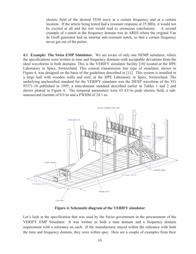
4.1 Example: The Swiss EMP Simulator. We are aware of only one NEMP simulator, where the specifications were written in time and frequency domains with acceptable deviations from the ideal waveforms in both domains. This is the VERIFY simulator facility [10] located at the HPE Laboratory in Spiez, Switzerland. This conical transmission line type of simulator, shown in Figure 4, was designed on the basis of the guidelines described in [11]. This system is installed in a large hall with wooden walls and roof, at the HPE Laboratory in Spiez, Switzerland. The underlying unclassified standard for the VERIFY simulator was the DEXP waveform of the VG 95371-10 published in 1995, a time-domain standard described earlier in Tables 1 and 2 and shown plotted in Figure 4. The temporal parameters were 65 kV/m peak electric field, a sub-nanosecond risetime of 0.9 ns and a FWHM of 24.1 ns.

Figure 4. Schematic diagram of the VERIFY simulator

Let’s look at the specification that was used by the Swiss government in the procurement of the VERIFY EMP Simulator. It was written as both a time domain and a frequency domain requirement with a tolerance on each. If the manufacturer stayed within the tolerance with both the time and frequency domain, they were within spec. Here are a couple of examples from their

11

specification. The time-domain specifications are illustrated in Figures 5 and 6 using the waveform and its time derivative.

Figure 5. Time-domain Specification for the VERIFY Simulator. The peak and FWHM are specified within a defined tolerance

Figure 6. Using the derivative to define the risetime

12

The specification on the spectral domain for the VERIFY simulator was prescribed as:

“In the frequency range from DC to 500 MHz, the spectral amplitude densities shall not deviate more than + 6 dB from the theoretical spectrum of the double exponential pulse given in paragraph _____, and not more than + 12 dB in the frequency range from 500 MHz to 1 GHz.”

In other words, the ideal time domain waveform has a well-defined spectrum and the simulated spectrum has error bars defined by the above statement. While the actual acceptable deviations from the ideal in the spectral domain are subjective numbers, the prescription of the deviation is deemed essential. 5. Proposed Format for Specifications

This is a format that we recommend for the electromagnetic specifications of NEMP simulator.

Electromagnetic Specification

5.1 Range of Field Levels (electric and magnetic) in the Working Volume

5.2 Voltage Range of Pulse Generator

5.3 Limits on Load Impedance Mismatch on the generator

5.4 Antenna Type (Radiating, Guided wave, Hybrid) and Polarization of the Electric Field

5.5 Polarity

5.6 Pulse Repetition Rate

5.7 Pulse to Pulse Reproducibility

5.8 Tolerable Field Levels around the simulator, if this is a concern to nearby facilities

5.9 Field Characterization in the Working Volume

This is where the particular temporal NEMP Standard (classified or unclassified) will be specified as an ideal waveform.

The 100% value (E100 or H100) is defined as the value of the field measured in any point in the working volume where the first derivative of the field is zero or has a first local minimum after the peak of the derivative.

Note: that this simulator produces a spherical TEM wave in the conic section which is automatically ~ 377�. It is not necessary to specify the wave impedance.

13

Note: In this kind of geometry, the characteristic impedance of free space, Zo ~ 377� is defined by the medium, o and o. The impedance of the transmission line is different, ZL = [V/ I] at any point in the transmission line � Zo. One should not confuse the two.

5.10 Prepulse The amplitude of the prepulse at any time has to be less than say 10% of the 100% value of the measured field.

5.11 Risetime (see Figures 5 and 6)

Example # 1 specification: The risetime Tr is defined as the time duration, in which the field increases from the time t10, where the field level is 10% of the measured 100% value(E100 or H100), to t90, where the field level is 90% of the measured 100% value (E100 or H100).

Example # 2 specification: Use tmr defined in equation (4) above.

All the following conditions have to be met:

a) Tr = prescribed by the standard within certain specified tolerance limits

b) During the risetime Tr of the pulse no glitches are allowed, the first derivative shall be always positive.

c) During the risetime Tr the second derivative shall be continuously positive during the rise of the first derivative, then continuously negative during the decay of the first derivative.

5.12 Pulse duration and Decay (see Figures 5 and 6)

FWHM = prescribed by the standard with acceptable tolerances

A double exponential curve shall be fitted through the three measured values E50i , E100 , E50d or H50i , H100 , H50d respectively. At any time after the 100% value (E100 or H100) the measured value of the amplitude has to follow the fitted double exponential within �10% of the100% value (E100 or H100).

5.13 Field Uniformity specifications In any point in the working volume the following shall be met:

a) The peak amplitude of electric or magnetic field shall not deviate more than � X % of its value at the geometric center of that plane.

b) The rising portion of the pulse has to meet the pre-pulse and risetime conditions.

c) The decaying portion has to meet the FWHM specification above.

d) The 1/r fall-off of the fields in the working volume due to the distance r of the generator is to be expected and there shall be no other losses..

5.14 Spectrum In the frequency range from DC or a suitable low frequency to 500 MHz the spectral amplitude densities shall not deviate more than � Y % from the theoretical spectrum of the double exponential pulse and not more than � Z % in the frequency range from 500 MHz to 1 GHz.

14

5.15 Working Volume Definition This is based on where the electromagnetic fields are best, not on where one can most conveniently access. As an example, in the ARES type simulator (see Figure 7) this is defined as the region above the first bend, not the center of the parallel-plate region (due to the diffraction of the wave at that first bend).Similarly for the case of the distributed terminator (as in VERIFY) the working volume should not be too close to the terminator (on the order of one plate height away) where the fields can be significantly distorted. This should all be specified.

Figure 7. The desired working volume is under the first bend in ARES type of simulator avoiding the diffraction zones

5.16 Simulator-Test Object Interaction As discussed in [11], the presence of the simulator structure alters the response of the test object due to scattering back and forth between the test object and the simulator structure. One needs to specify the allowed deviation of the currents/charges on the test object (from the case of the ideal uniform incident plane wave). Typically 25% has been allowed giving a requirement of plate spacing as 1.6 h for missile-like test objects of height h [12]. The allowed deviation should be specified.

5.17 Terminator Reflections.This reflection needs to be kept below specified amount (say 10% or so) at the working volume in both time and frequency domains. This can be measured by taking appropriate weighted sum and difference of electric and magnetic field waveforms, described in [13].

15

It is noted that we have focused on the electromagnetic specifications above and that there shall be other specifications such as:

� Limitations on the location and size of the facility

� Weight and Transportability of Generator

� Operating/Storage Temperature Range

� Power Supply

� Prohibited Insulation Materials

� Computer /Remote Control operation of the Pulser

� Safety Issues

� Pulse Counter

� Reliability and Maintenance

� Spare Parts

� Acceptance Test Procedure

� Deliverables

The specific type of simulator such as (a) Guided Wave, (b) Radiating or (c) Hybrid will have to be considered and the above format of the specification suitably modified. For example, in the radiating type of simulator, the low frequencies will be severely limited and this can be easily addressed while writing the specifications. The main point here is the inclusion of the temporal and spectral specifications with acceptable tolerances.

16

APPENDIX A

Examples of NEMP Simulators Classification of NEMP Simulators

Since the 1960s, when the early NEMP facilities were built, it has been recognized that there are basically three types of NEMP simulators. They are the guided wave, the radiating type and the hybrid that combines some aspects of both radiating type and the guided wave types of simulators. We now discuss the salient features of all three types of simulating the NEMP environment. A.1 Guided Wave Simulators. A number of Guided Wave simulators have been built, including ALECS, ARES, NOTES, and of course, the famous ATLAS-I (Trestle), shown in Figure A.1. Sometimes these simulators are erroneously called the “bounded wave” simulators. Strictly speaking, the electromagnetic wave is guided between two conductors, but it is not bounded. There is leakage of electromagnetic fields around the facility. However, most of the energy is contained between the plates, and that is probably where the name came from.

Figure A-1. ATLAS-I (Trestle) Simulator

ATLAS-I is a horizontally polarized, horizontally propagating, parallel-plate transmission line type of simulator.

A.2 Radiating Simulators

ATHAMAS II seen in Figure A-2 is a resistively loaded mono-cone radiator producing a vertically polarized NEMP simulation. ATHAMAS II has also been used in EMP tests in an aircraft fly-by mode. NAVES / EMPRESS seen in Figure A-3 was similar to ATHAMAS-II, except it was built on a barge out on the sea, designed for EMP testing of ships.

17

Figure A.2. ATHAMAS-II resistively loaded radiating mono-cone simulator

Figure A-3. NAVES/EMPRESS Simulator Similar to ATHAMAS II, but on a Barge

A.3 Hybrid Simulators

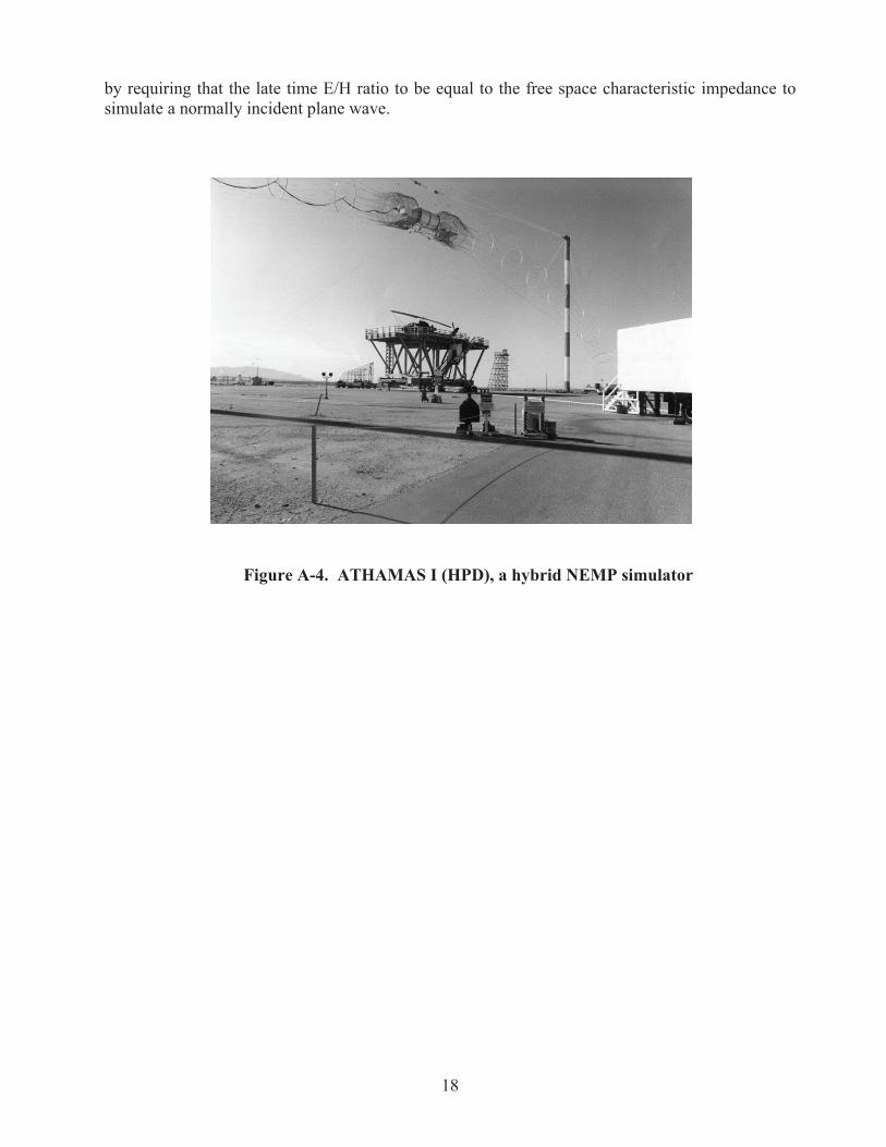
The ATHAMAS-I seen in Figure A.4 is an elliptical loop type of simulator with a largely horizontal electric field simulation. It is called the hybrid type, simply because it combines some aspects of both radiating and guided wave simulators. The very early time simulated field comes directly from the biconical pulser and the late time fields are maintained by the currents flowing on the loaded elliptical structure The loading (~ 614 Ohms total or 307 Ohms per side) is computed

18

by requiring that the late time E/H ratio to be equal to the free space characteristic impedance to simulate a normally incident plane wave.

Figure A-4. ATHAMAS I (HPD), a hybrid NEMP simulator

19

References

[1] IEC 61000 2-9, “Electromagnetic compatibility (EMC) - Part 2: Environment - Section 9: Description of HEMP environment - Radiated disturbance. Basic EMC publication”, can be purchased at http://webstore.iec.ch

[2] C.E. Baum, “Some Considerations Concerning Analytic EMP Criteria Waveforms,”

Theoretical Note 285, October 1976. [3] EMP Engineering and Design Principles, Electrical Protection Department, Bell Telephone Laboratories, 1975. [4] C.E. Baum, “From the Electromagnetic Pulse to High-Power Electromagnetics,” Proc. IEEE, Vol. 80, No. 6, June 1992, pp. 789-817. [5] International Electrotehnical Commission, IEC-77C from M. Wik, Presentation at EUROREM 94, Bordeaux, France, July 1994. [6] K-D. Leuthäuser, “A Complete EMP Environment Generated by High-Altitude Nuclear

Bursts: Data and Standardization,” Theoretical Note 364, Air Force Phillips Laboratory, February 1994.

[7] VG95371-10 from Bundesamt für Wehrtechnik und Beschaffung, Germany (replaces Edition 1993-08). [8] “Electromagnetic Environmental Effects Requirements for Systems,” MIL-STD-464A,

December 19, 2002. [9] IEC 61000 4-32, “Electromagnetic compatibility (EMC) - Part 4-32: Testing and

measurement techniques - High-altitude electromagnetic pulse (HEMP) simulator compendium”, can be purchased at http://webstore.iec.ch

[10] M. Nyffeler, A. Jaquier, B. Reusser, P-F. Bertholet, and A. W. Kaelin, “VERIFY, a Threat

Level NEMP Simulator with a 1ns Risetime,” presentation at AMEREM 2006, Albuquerque NM, July 2006.

[11] D. V. Giri and C. E. Baum, “Design Guidelines for Flat-Plate Conical Guided-Wave EMP

Simulators with Distributed Terminators,” Sensor and Simulation Note 402, Air Force Research Laboratory, 25 October 1996.

[12] C. D. Taylor and G. A. Steigerwald, “On the Pulse Excitation of a Cylinder in a Parallel Plate Waveguide,” Sensor and Simulation Note 99, Air Force Weapons Laboratory, March 1970. [13] D. V. Giri, T. K. Liu, F. M. Tesche, and R. W. P. King, “Parallel Plate Transmission Line Type of EMP Simulators: A Systematic Review and Recommendations,” LuTech Inc., and Harvard University, Sensor and Simulation Note 261, Air Force Weapons Laboratory April 1980.