225FEBRUARY 2005AMERICAN METEOROLOGICAL SOCIETY |

T

AFFILIATIONS: LAWRENCE—Junior Research Group, Departmentof Atmospheric Chemistry, Max Planck Institute for Chemistry,Mainz, GermanyCORRESPONDING AUTHOR: Mark G. Lawrence, Max PlanckInstitute for Chemistry, Junior Research Group, Department ofAtmospheric Chemistry, Postfach 3060, 55020 Mainz, GermanyE-mail: lawrence@mpch-mainz.mpg.deDOI:10.1175/BAMS-86-2-225

In final form 22 July 2004©2005 American Meteorological Society

(1)

or

(2)

where t and td are in degrees Celsius and RH is inpercent. In this article I first give an overview of themathematical basis of the general relationship be-tween the dewpoint and relative humidity, and con-sider the accuracy of this and other approximations.Following that, I discuss several useful applicationsof the simple conversion, and conclude with a briefperspective on the early history of research in thisfield.

DEFINITIONS AND ANALYTICAL RELA-TIONSHIPS. Relative humidity is commonly de-fined in one of two ways, either as the ratio of the ac-tual water vapor pressure e to the equilibrium vaporpressure over a plane of water es (often called the“saturation” vapor pressure),

The Relationship between RelativeHumidity and the DewpointTemperature in Moist AirA Simple Conversion and Applications

BY MARK G. LAWRENCE

How are the dewpoint temperature and relative humidity related, and is there an easy

and sufficiently accurate way to convert between them without using a calculator?

he relative humidity (RH) and the dewpointtemperature (td) are two widely used indicatorsof the amount of moisture in air. The exact con-

version from RH to td, as well as highly accurate ap-proximations, are too complex to be done easily with-out the help of a calculator or computer. However,there is a very simple rule of thumb that I have foundto be quite useful for approximating the conversionfor moist air (RH > 50%), which does not appear tobe widely known by the meteorological community:td decreases by about 1°C for every 5% decrease in RH(starting at td = t, the dry-bulb temperature, when RH= 100%):

226 FEBRUARY 2005|

, (3)

or as the ratio of the actual water vapor dry mass mix-ing ratio w to the equilibrium (or saturation) mixingratio ws at the ambient temperature and pressure:

(4)

The two definitions are related by w = ee(P - e)-1 andws = ees(P - es)

-1, where e(0.622) is the ratio of the mo-lecular weights of water and dry air, and P is the am-bient air pressure. For many applications, the twodefinitions in Eqs. (3) and (4) are essentially equiva-lent, because normally e < es P; however, as will beshown below, in cases such as the dewpoint whereexponentials are involved, the difference can becomenonnegligible. The temperature to which an air par-cel at initial temperature t and pressure P must becooled isobarically to become saturated is td (i.e., theinitial mixing ratio w, which is conserved, equals wsat the new temperature td). Normally the definitionis expressed implicitly in terms of the vapor pressure

(5)

To express td in terms of RH, an expression for thedependence of es on t is needed. Over the past twocenturies, an immense number of such expressionshave been proposed (probably exceeding 100), bothon empirical and theoretical bases. A nice review andevaluation of many of these is given by Gibbins (1990).One of the most widely used, highly accurate empiri-cal expressions is

(6)

which is commonly known as the Magnus formula,although, as discussed below, this is a rather inaccu-rate attribution. Alduchov and Eskridge (1996) haveevaluated this expression based on contemporary va-por pressure measurements and recommend the fol-lowing values for the coefficients: A1 = 17.625, B1 =243.04°C, and C1 = 610.94 Pa. These provide valuesfor es with a relative error of < 0.4% over the range-40°C £ t £ 50°C.

Substituting Eq. (6) in Eq. (5) yields td as a func-tion of the ambient vapor pressure and temperature

(7)

Combining this with Eq. (3) then gives

(8)

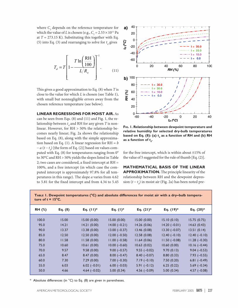
which is a highly accurate conversion from RH to td,provided that RH is defined using Eq. (3); the errorthat results if Eq. (4) is used is discussed below. Therelationship between td, t, and RH based on Eq. (8) isshown in Fig. 1, with sample values in Table 1. Thisconversion, broken down into multiple steps, witholder coefficients (from Tetens 1930), was recentlyrecommended for public use in a nice compilation ofseveral humidity formulas (USA Today, 6 November2000, currently available online at www.vivoscuola.it/u s / r s i gpp3202 /um id i t a / a t t i v i t a / humid i t y_formulas.htm, or from the author on request).

A simpler, well-known analytical form for es canbe obtained by solving the Clausius–Clapeyron equa-tion,

(9)

where T is the temperature in Kelvin (T = t + 273.15),Rw is the gas constant for water vapor (461.5 J K-1 kg-1),and L is the enthalpy of vaporization, which variesbetween L = 2.501 ¥ 106 J kg-1 at T = 273.15 K and L= 2.257 ¥ 106 J kg-1 at T = 373.15 K. Assuming that Lis approximately constant over the temperature rangeencountered in the lower atmosphere allows Eq. (9)to be integrated to yield

(10)

227FEBRUARY 2005AMERICAN METEOROLOGICAL SOCIETY |

where C2 depends on the reference temperature forwhich the value of L is chosen (e.g., C2 = 2.53 ¥ 1011 Paat T = 273.15 K). Substituting this together with Eq.(5) into Eq. (3) and rearranging to solve for td gives

T TT

L Rdw

= −

−

1

1

ln.

RH100

(11)

This gives a good approximation to Eq. (8) when T isclose to the value for which L is chosen (see Table 1),with small but nonnegligible errors away from thechosen reference temperature (see below).

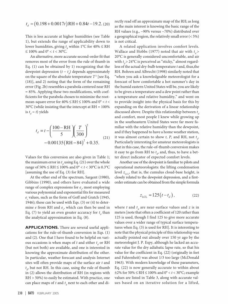
LINEAR REGRESSIONS FOR MOIST AIR. Ascan be seen from Eqs. (8) and (11) and Fig. 1, the re-lationship between td and RH for any given T is non-linear. However, for RH > 50% the relationship be-comes nearly linear; Fig. 2a shows the relationshipbased on Eq. (8), along with the simple approxima-tion based on Eq. (1). A linear regression for RH = b- a (t - td) [the form of Eq. (2)] based on values com-puted with Eq. (8) for temperatures ranging from 0°to 30°C and RH > 50% yields the slopes listed in Table2; two cases are considered, a fixed intercept at RH =100%, and a free intercept (in which case the com-puted intercept is approximately 97.8% for all tem-peratures in this range). The slope a varies from 4.62to 5.81 for the fixed intercept and from 4.34 to 5.45

for the free intercept, which is within about ±15% ofthe value of 5 suggested for the rule of thumb [Eq. (2)].

MATHEMATICAL BASIS OF THE LINEARAPPROXIMATION. The principle linearity of therelationship between RH and the dewpoint depres-sion (t - td) in moist air (Fig. 2a) has been noted pre-

FIG. 1. Relationship between dewpoint temperature andrelative humidity for selected dry-bulb temperaturesbased on Eq. (8): (a) td as a function of RH and (b) RHas a function of td.

100.0 15.00 15.00 (0.00) 15.00 (0.00) 15.00 (0.00) 15.10 (0.10) 15.75 (0.75)95.0 14.21 14.21 (0.00) 14.00 (-0.21) 14.26 (0.06) 14.20 (-0.01) 14.63 (0.43)90.0 13.37 13.38 (0.00) 13.00 (-0.37) 13.46 (0.08) 13.30 (-0.07) 13.51 (0.14)

85.0 12.50 12.50 (0.00) 12.00 (-0.50) 12.58 (0.08) 12.40 (-0.10) 12.40 (-0.10)80.0 11.58 11.58 (0.00) 11.00 (-0.58) 11.64 (0.06) 11.50 (-0.08) 11.28 (-0.30)75.0 10.60 10.61 (0.00) 10.00 (-0.60) 10.63 (0.02) 10.60 (0.00) 10.16 (-0.44)70.0 9.57 9.58 (0.00) 9.00 (-0.57) 9.55 (-0.02) 9.70 (0.13) 9.04 (-0.53)65.0 8.47 8.47 (0.00) 8.00 (-0.47) 8.40 (-0.07) 8.80 (0.33) 7.93 (-0.55)60.0 7.30 7.29 (0.00) 7.00 (-0.30) 7.19 (-0.10) 7.50 (0.20) 6.81 (-0.49)

55.0 6.03 6.02 (-0.01) 6.00 (-0.03) 5.91 (-0.12) 6.25 (0.22) 5.69 (-0.34)50.0 4.66 4.64 (-0.02) 5.00 (0.34) 4.56 (-0.09) 5.00 (0.34) 4.57 (-0.08)

TABLE 1. Dewpoint temperatures (°C) and absolute differences for moist air with a dry-----bulb tempera-ture of t = 15°C.

RH (%) Eq. (8) Eq. (11)* Eq. (1)* Eq. (21)* Eq. (19)* Eq. (20)*

* Absolute differences (in °C) to Eq. (8) are given in parentheses.

228 FEBRUARY 2005|

viously, for instance, by Sargent (1980) on an empiri-cal basis, and theoretically by Bohren and Albrecht(1998). In particular, Bohren and Albrecht (1998)made use of this to explain why dewpoint is often pre-ferred by meteorologists over relative humidity as anindicator of human comfort. Their approach to show-ing the linear nature of the curves in the moist regimebegins by rearranging Eq. (11) to solve for RH (here,following their derivation, the absolute temperatureT and the absolute dewpoint Td will be used forconvenience):

(12)

When the exponent satisfies the condition

(13)

the exponential can be approximated by a Taylor ex-pansion, discarding the second- and higher-orderterms:

(14)

which can be rewritten in the form of Eq. (2), with thedewpoint depression expressed in degrees Celsius

(15)

where

(16)

Because T and Td only vary by about 10% in the tem-perature regime that is mainly of interest (around270–300 K), b1 is nearly constant, and, thus, the rela-tionship between RH and t - td in Eq. (15) is nearlylinear. Assuming Td ª T, this gives b1 ª 6.0 for T =300 K and b1 ª 7.4 for T ª 270 K [note that Bohrenand Albrecht (1998) did not compute values for b1,because they were mainly concerned with the quali-tative form of the relationship]. These are somewhatlarger in magnitude than the linear regression slopesin Table 2. This is because the assumption in Eq. (13)applies best near saturation; for a typical temperatureof T = 285 K, Eq. (13) reduces to approximately0.07 (T - Td) = 1, which only holds well if T - Td �

30 4.34 4.6225 4.50 4.7920 4.67 4.9715 4.85 5.1610 5.03 5.375 5.24 5.580 5.45 5.81

TABLE 2. Slopes (a, in % °C-----1) of the linearregression RH = b ----- a (t ----- td) = (b ----- at) +++++ atd forthe curves in Fig. 2a, based on the valuescomputed with Eq. (8), for a free intercept band for a fixed intercept at RH = b = 100%.

t (°C) b = free b = 100

FIG. 2. (a) Relationship between td and RH for moist air;thick colored broken lines show values based on Eq. (8)for selected dry-bulb temperatures with line styles asin Fig. (1), thin solid black lines show values based onEq. (1); and (b) difference between td computed withEq. (1) minus values from Eq. (8) for selected dry-bulbtemperatures with line styles as in Fig. (1), where col-ored curves show values computed using Eq. (3) for RHand gray curves show values using Eq. (4) for RH as-suming an air pressure of P = 1013 hPa.

n

229FEBRUARY 2005AMERICAN METEOROLOGICAL SOCIETY |

3 K; this is about 1/3 of the overall quasi-linear range,which extends up to a dewpoint depression of about10 K (Fig. 2a).

A more accurate expression for the slope tangentto any point in the RH versus t - td relationship canbe obtained by dividing both sides of Eq. (11) by (100- RH) and rearranging to obtain

(17)

where

(18)

The magnitude of the slope is now seen to decreasewith RH; it also decreases for higher values of T (asdoes b1). At RH = 50%, this gives b2 ª 4.3 for T = 300 Kand b2 ª 5.4 for T = 270 K; thus, the overall slopes us-ing Eqs. (17) and (18) are in accord with the linearregressions in Table 2. Note that it is also possible toobtain nearly the same expression as in Eqs. (17) and(18) by using the series expansion 1(1 - x)-1 =1 + x +x2 + . . . directly on Eq. (11), and discarding the sec-ond- and higher-order terms, which is valid to do overa larger range of dewpoint depressions than the ap-proximation in Eq. (13).

ACCURACY AND OTHER APPROXIMA-TIONS. How accurate is the simple conversion inEqs. (1) and (2)? Sample values for Eq. (1) for t = 15°Care given in Table 1, and the error in the rule ofthumb relative to Eq. (8) is plotted in Fig. 2b for arange of temperatures. Generally, the conversion isaccurate to better than 1°C for td or 5% for RH formost of the range 0° < t < 30°C and 50% < RH < 100%,with exceptions at the extreme temperatures. To anextent, the largest errors can be compensated for bynoting the form of the error in Fig. 2b (e.g., subtract-ing 1°C for t ª 30°C and RH � 60%, and adding 1°Cfor t ª 0°C and RH � 80%). When a high degree ofaccuracy (� 1% error) is required, for example, formodeling, publication of tables or current weather re-ports, then this simple conversion is clearly inad-equate. However, there are several applications forwhich this accuracy is sufficient that the rule ofthumb can be very useful, as discussed in the nextsection.

The values in Table 1 are computed using Eq. (3)for the definition of RH. With this definition, Eq. (8)provides an accurate conversion over a wide range oftemperatures, as does Eq. (11) near the chosen refer-ence temperature (the values in Table 1 were computedwith L = 2.472 ¥ 106 J kg-1, appropriate for a referencetemperature of T = 285 K). If instead Eq. (4) is usedfor RH, and an air pressure of P = 1013 hPa is as-sumed, then generally slightly smaller errors are com-puted for the rule-of-thumb conversion in Eq. (1); thisis illustrated in Fig. 2b (gray curves). However, inter-estingly, when Eq. (4) is used, then directly using Eqs.(8) and (11) [i.e., assuming es = P, so that Eqs. (3) and(4) are equivalent] can lead to notable errors, com-pared with the accurate values computed by insteadsubstituting Eq. (4) and e = (wP)(w + e)-1 into Eq. (7),particularly at the lowest values of RH considered. ForRH = 50%, the error in Eq. (8) applied with Eq. (4)ranges from -0.04°C at t = 0°C to -0.34°C at t = 30°C(i.e., up to ~3% of the dewpoint depression), while theerror in Eq. (11) together with Eq. (4) is smallest at -0.14°C for t = 10°–15°C (near the chosen referencetemperature of t = 285 K), increasing in magnitudeto -0.23°C at t = 30°C and -0.17°C at t = 0°C. Theseerrors can be contrasted with the maximum error forEq. (11) when Eq. (3) is used for RH, which is -0.13°Cat t = 0°C. Thus, if Eq. (4) is used to define RH, andan accurate conversion is needed, then e should firstbe computed [using Eq. (4) and e = (wP)(w + e)-1] andthen used in Eq. (7) to determine td, rather than di-rectly employing Eqs. (8) or (11) with the given RH.

For cases where the rule of thumb in Eq. (1) is notadequately accurate, but a simpler conversion thanEqs. (7), (8), or (11) is desired, then various other ap-proximations that have been proposed can be used.Sargent (1980) gives a nice overview of a wide rangeof approximations of various accuracies. In particu-lar, he proposes an empirical linear fit that has thesame basic form as Eq. (1):

(19)

where K0 = 17.9 and K1 = 0.18 for 65% £ RH £ 100%,and K0 = 22.5 and K1 = 0.25 for 45% £ RH £ 65%.These are close to the equivalent values for the ruleof thumb of K0 = 20 and K1 = 0.2 in Eq. (1), but yielda clearly more accurate conversion due to the two-part fit to the slope (see Table 1). However, Sargent’sconversion is already sufficiently complex to be pro-hibitive for being used “on the fly.” Sargent (1980) alsoproposed a higher-order fit, which includes a depen-dence on the temperature:

230 FEBRUARY 2005|

(20)

This is less accurate at higher humidities (see Table1), but extends the range of applicability down tolower humidities, giving td within 1°C for 40% £ RH£ 100% and 0° < t < 30°C.

An alternative, more accurate second-order fit thatremoves most of the error from the rule of thumb inEq. (1) can be obtained by 1) recognizing that thedewpoint depression (t - td) depends approximatelyon the square of the absolute temperature T 2 [see Eq.(18)], and 2) noting that the form of the remainingerror (Fig. 2b) resembles a parabola centered near RH= 85%. Applying these two modifications, with coef-ficients for the parabola chosen to minimize the root-mean-square error for 40% £ RH £ 100% and 0° < t <30°C (while insisting that the intercept at RH = 100%is td = t) yields

(21)

Values for this conversion are also given in Table 1;the maximum error in td using Eq. (21) over the wholerange of 50% £ RH £ 100% and 0° < t < 30°C is 0.3°C[assuming the use of Eq. (3) for RH].

At the other end of the spectrum, Sargent (1980),Gibbins (1990), and others have evaluated a widerange of complex expressions for es, most employingvarious polynomial and exponential fits for measuredes values, such as the form of Goff and Gratch (1945,1946); these can be used with Eqs. (3) or (4) to deter-mine e from RH and es, which can then be used inEq. (7) to yield an even greater accuracy for td thanthe analytical approximation in Eq. (8).

APPLICATIONS. There are several useful appli-cations for the rule-of-thumb conversion in Eqs. (1)and (2). One that I have found to be helpful on vari-ous occasions is when maps of t and either td or RH(but not both) are available, and one is interested inknowing the approximate distribution of the other.In particular, weather forecast and analysis Internetsites will often provide maps of the surface air t andtd, but not RH. In this case, using the rule of thumbin (2) allows the distribution of RH (in regions withRH > 50%) to easily be estimated. With practice, onecan place maps of t and td next to each other and di-

rectly read off an approximate map of the RH; as longas the main interest is knowing the basic range of theRH values (e.g., ~90% versus ~70%) distributed overa geographical region, the relatively small error (< 5%)is not critical.

A related application involves comfort levels.Wallace and Hobbs (1977) noted that air with td >20°C is generally considered uncomfortable, and airwith td > 24°C is perceived as “sticky,” almost regard-less of the actual dry-bulb temperature t and, thus,theRH. Bohren and Albrecht (1998) similarly noted that“when you ask a knowledgeable meteorologist for aforecast of how comfortable a hot summer’s day inthe humid eastern United States will be, you are likelyto be given a temperature and a dew point rather thana temperature and relative humidity,” and went onto provide insight into the physical basis for this byexpanding on the derivation of a linear relationshipdiscussed above. Despite this relationship between tdand comfort, most people I knew while growing upin the southeastern United States were far more fa-miliar with the relative humidity than the dewpoint,and if they happened to have a home weather station,it was almost certain to show t, P, and RH, not td.Particularly interesting for amateur meteorologists isthat in this case, the rule-of-thumb conversion makesit easy to go from RH to td, and, thus, to have a bet-ter direct indicator of expected comfort levels.

Another use of the dewpoint is familiar to pilots andoperational meteorologists: the lifting condensationlevel zLCL, that is, the cumulus cloud-base height, isclosely related to the dewpoint depression, and a first-order estimate can be obtained from the simple formula

, (22)

where t and td are near-surface values and z is inmeters [note that often a coefficient of 120 rather than125 is used, though I find 125 to give more accuratevalues over a wider range of typical surface tempera-tures when Eq. (3) is used for RH]. It is interesting tonote that the physical principle of this relationship wasactually pointed out already over 150 yr ago by themeteorologist J. P. Espy, although he lacked an accu-rate value for the dry adiabatic lapse rate, so that hisvalue for the coefficient in Eq. (22) (originally in feetand Fahrenheit) was about 1/3 too large (McDonald1963). With modern knowledge of these parameters,Eq. (22) is now generally accurate to within about±2% for 50% £ RH £ 100% and 0° < t < 30°C; examplevalues are listed in Table 3, along with accurate val-ues based on an iterative solution for a lifted,

231FEBRUARY 2005AMERICAN METEOROLOGICAL SOCIETY |

nonentraining parcel, for which Eq. (3) is used todefine RH. When Eq. (4) is instead used, notablylower values of zLCL are computed for both the itera-tive solution and Eq. (22), by 0.5% at t = 0°C, and upto 4% lower at t = 30°C.

Using the rule of thumb discussed here, this rela-tionship can be reformulated in terms of RH. Directlysubstituting Eq. (1) into Eq. (22) gives

. (23)

However, as can be seen in Fig. 2b, Eq. (1) tends tounderestimate td for lower temperatures, which re-sults in an overestimate of the cloud-base height us-ing Eq. (23). I have found that it is easy to adjust forthis tendency by incorporating the temperature intothe coefficient:

, (24)

where t here is the dry-bulb surface temperature indegrees Celsius. This gives zLCL to within ±15% for the

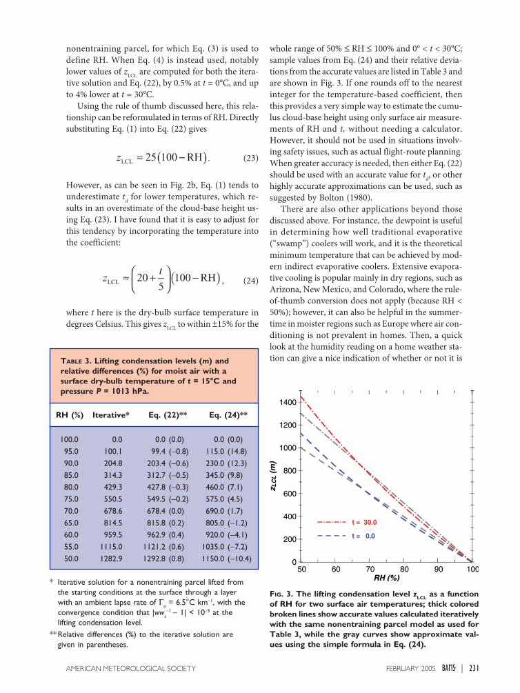
whole range of 50% £ RH £ 100% and 0° < t < 30°C;sample values from Eq. (24) and their relative devia-tions from the accurate values are listed in Table 3 andare shown in Fig. 3. If one rounds off to the nearestinteger for the temperature-based coefficient, thenthis provides a very simple way to estimate the cumu-lus cloud-base height using only surface air measure-ments of RH and t, without needing a calculator.However, it should not be used in situations involv-ing safety issues, such as actual flight-route planning.When greater accuracy is needed, then either Eq. (22)should be used with an accurate value for td, or otherhighly accurate approximations can be used, such assuggested by Bolton (1980).

There are also other applications beyond thosediscussed above. For instance, the dewpoint is usefulin determining how well traditional evaporative(“swamp”) coolers will work, and it is the theoreticalminimum temperature that can be achieved by mod-ern indirect evaporative coolers. Extensive evapora-tive cooling is popular mainly in dry regions, such asArizona, New Mexico, and Colorado, where the rule-of-thumb conversion does not apply (because RH <50%); however, it can also be helpful in the summer-time in moister regions such as Europe where air con-ditioning is not prevalent in homes. Then, a quicklook at the humidity reading on a home weather sta-tion can give a nice indication of whether or not it is

100.0 0.0 0.0 (0.0) 0.0 (0.0)95.0 100.1 99.4 (-0.8) 115.0 (14.8)90.0 204.8 203.4 (-0.6) 230.0 (12.3)85.0 314.3 312.7 (-0.5) 345.0 (9.8)80.0 429.3 427.8 (-0.3) 460.0 (7.1)75.0 550.5 549.5 (-0.2) 575.0 (4.5)70.0 678.6 678.4 (0.0) 690.0 (1.7)65.0 814.5 815.8 (0.2) 805.0 (-1.2)60.0 959.5 962.9 (0.4) 920.0 (-4.1)55.0 1115.0 1121.2 (0.6) 1035.0 (-7.2)50.0 1282.9 1292.8 (0.8) 1150.0 (-10.4)

TABLE 3. Lifting condensation levels (m) andrelative differences (%) for moist air with asurface dry-bulb temperature of t = 15°C andpressure P = 1013 hPa.

RH (%) Iterative* Eq. (22)** Eq. (24)**

* Iterative solution for a nonentraining parcel lifted fromthe starting conditions at the surface through a layerwith an ambient lapse rate of Ga = 6.5°C km-1, with theconvergence condition that |wws

-1 - 1| < 10-5 at thelifting condensation level.

** Relative differences (%) to the iterative solution aregiven in parentheses.

FIG. 3. The lifting condensation level zLCL as a functionof RH for two surface air temperatures; thick coloredbroken lines show accurate values calculated iterativelywith the same nonentraining parcel model as used forTable 3, while the gray curves show approximate val-ues using the simple formula in Eq. (24).

232 FEBRUARY 2005|

worth setting up a fan and a drying rack with wetlaundry in order to cool off at least a few degrees whenpossible, which we found to frequently be useful dur-ing the first part of the anomalously hot Europeansummer of 2003 [as can be seen from Eq. (1), assum-ing at best a 50% cooling efficiency from this primi-tive engineering, this is only worthwhile if RH £ 70%].

A final widely useful application for the simpleconversion is in science education. Most students arealready basically familiar with the relative humidity,and the rule of thumb provides a simple way to ex-tend this to having a feeling for the meaning ofdewpoint temperatures and dewpoint depressions.This provides a particularly nice insight when stu-dents then link this to cloud-base levels through Eq.(24), which can be put into practice outside on dayswith appropriate weather conditions.

HISTORICAL PERSPECTIVE. Practical relation-ships involving the humidity parameters td (or t - td)and RH have long been of interest, and several dif-ferent approximate conversions have been proposed,most notably the empirical linear fit in Eq. (19) fromSargent (1980), which is similar to Eq. (1). Neverthe-less, despite a rather extensive search through recentand historical literature, as well as on the Internet, Ihave not yet been able to find mention of the simplerule of thumb and its applications as discussed here.

The earliest recorded careful measurements of thedewpoint that I could find were made by Dalton(1802), who was interested in understanding the pro-cess of evaporation of liquid water into moist air. Hesuspected that the rate of evaporation depended onthe temperature, which determines the equilibriumvapor pressure (es) of the liquid water, as well as themoisture content of the ambient air (which he calledthe “force of the aqueous atmosphere”). To quantifythis moisture content, he filled a glass with cold springwater and watched to see if dew formed on the out-side. If so, he poured out the water, let it warm up abit, dried off the glass, and poured the water back in,repeating this until the first time that dew did notform; measuring the temperature of the water in theglass gave him the dewpoint (Dalton called this the“condensation point”). He then used his new table ofes as a function of temperature (also published in thesame work) to determine the vapor pressure in am-bient air, reasoning (correctly) that this would beequal to es at the dewpoint temperature. Finally, heperformed a large set of experiments in which hemeasured the rate of evaporation of water at differenttemperatures in a small tin container, using a balanceto determine the change in weight, and found that the

rate of evaporation was indeed proportional to the dif-ference between es at the temperature of the water inthe container and the vapor pressure in the ambient air.

John Dalton’s experimental technique and his in-sights in this field were remarkable. His vapor pres-sure measurements were accurate enough to allowhim to realize that es approximately doubled for ev-ery 22.5°F increase in temperature, and that the ratiodecreased with increasing temperature (from 2.17 at32°F to 1.59 at 212°F). This same reasoning was usedby August (1828) in proposing the formula that latercame to be known as the “Magnus formula” [Eq. (6)].Gibbins (1990) also noted that G. Magnus was not thefirst to suggest the Magnus formula, but that thishonor apparently belongs to E. F. August. I would gofurther and propose that Eq. (6) should properly becalled the “August–Roche” or the “August–Roche–Magnus” formula (with possible coattribution toStrehlke, as well). Magnus (1844) made a very care-ful set of measurements of the equilibrium vapor pres-sure of water, which he desired to fit with a usableequation. He considered several different forms thathad previously been proposed, and came to the mainconclusion that the form of Eq. (6) was the best(author’s translation of the original German follows):“The form which is used by the French Academy andby Th. Young, Creighton, Southern,Tredgold, andCoriolis, and also by the authors of the entry for Steamin the Encyclopaedia Brittannica [sic] . . . regardlessof the exponential coefficients one may choose . . . isnot as good as the form suggested by Roche, August(1828), and Strehlke, which has also been arrived atthrough theoretical considerations by von Wrede(1841),” which is Eq. (6). So it was clear to Magnusthat attribution for the equation at least in part be-longed to August (1828), the only one of the threeearly investigators for which Magnus gives a refer-ence. The original form of the equation proposed byAugust used a base-10 logarithm, with A1 = 7.9817243,which becomes A1 = 18.3786 when converted to theappropriate value for the form of Eq. (6); for the othercoefficients he proposed that B1 = 213.4878°C and C1= 2.24208 mm Hg. The values of A1 and B1 are not sofar off from the values later recommended by Magnus(1844), A1 = 17.1485 (7.4475 in base 10) and B1 =234.69°C, although C1 was considerably lower thanMagnus’ value of 4.525 mm Hg. After Magnus (1844),and prior to more recent works like Alduchov andEskridge (1996), the most notable update of thesevalues was by Tetens (1930), who suggested that A1 =17.27 (7.5 in base 10), B1 = 237.3°C, and C1 = 610.66 Pa.

So August clearly deserves at least shared attribu-tion for this equation. Who were the others, though,

233FEBRUARY 2005AMERICAN METEOROLOGICAL SOCIETY |

that Magnus mentions? I have not been able to findany evidence of Strehlke’s work associated with this(any tips from readers would be appreciated). VonWrede (1841) independently comes across nearly thesame form, except without C1 in the equation, and,thus, quite different coefficients A1 and B1; he wasapparently unaware of August’s work, and mentionsin a footnote that he had not been able to obtain a copyof Roche’s work, which he had been told proposed asimilar formula. The reason for this was made clearerby Magnus (1844) a few years later, who noted that(author’s translation follows) “Roche had attemptedto propose such a theoretical formula, yet the reportfor the French Academy of Sciences (1830) said that,based on the available evidence, the formula wouldnot have the pleasure of the applause of the physi-cists.” [The original report in French does, indeed,read rather similarly.] Nevertheless, the extensive his-torical account in the entry on steam in theEncyclopaedia Britannica (1830–1842 ed.) of that pe-riod lists about 20 equations for es(t), including thatof Roche, who “sent to the Academy of Sciences, in1828, a memoir on this subject” [here they do notmention its fate; it is also difficult to determine whatthe coefficients Roche actually proposed were, be-cause the equation is given differently in theEncyclopaedia Britannica (1830–1842 ed., s.v.“steam”) and in the French Academy of Sciences(1830) report, though they are apparently signifi-cantly different from those of August and his succes-sors]. Surprisingly, however, the authors in theEncyclopaedia Britannica (1830–1842 ed., s.v.“steam”) do not mention the work of August (1828);this might help to explain why it was neglected, andwhy credit was instead later given to Magnus (1844).

Given the long history of research on atmosphericmoisture, it is hard to imagine that the simple ruleof thumb presented here for relating td, t, and RH, aswell as the simple computation of zLCL from t and RHin Eq. (24), have gone unnoticed. I would certainlyappreciate any information from colleagues or fromscience historians on whether earlier works can befound in which this rule of thumb is discussed.Nevertheless, these approximations seem to havebeen either generally overlooked or forgotten—atleast they are not widely known in this age of thepocket calculator and laptop (perhaps already sincethe slide rule)—and I hope that this article will helpto bring them to the attention of the various commu-nities that could benefit from their use, includingoperational meteorologists, amateur meteorologists,atmospheric scientists in various specializations, andscience educators.

ACKNOWLEDGMENTS. I would like to expressmy appreciation to Craig Bohren for very helpful commentsthroughout the development of this manuscript. The as-sistance of Andreas Zimmer in obtaining the historical ar-ticles is gratefully acknowledged. This work was supportedby the German Ministry for Education and Research(BMBF) Project 07ATC02.

REFERENCESAlduchov, O. A., and R. E. Eskridge, 1996: Improved

Magnus form approximation of saturation vaporpressure. J. Appl. Meteor., 35, 601–609.

August, E. F., 1828: Ueber die Berechnung derExpansivkraft des Wasserdunstes. Ann. Phys. Chem.,13, 122–137.

Bohren, C., and B. Albrecht, 1998: Atmospheric Thermo-dynamics. Oxford University Press, 402 pp.

Bolton, D., 1980: The computation of equivalent poten-tial temperature. Mon. Wea. Rev., 108, 1046–1053.

Dalton, J., 1802: On the force of steam or vapour fromwater and various other liquids, both in a vacuum andin air. Mem. Lit. Philos. Soc. Manchester, 5, 550–595.

French Academy of Sciences, 1830: Exposé des recherchesfaites par ordre de l’Académie royale des Sciences, pourdeterminer les forces élastiques de la vapeur d’eau à dehautes températures. Ann. Chim. Phys., 43, 74–112.

Gibbins, C. J., 1990: A survey and comparison of rela-tionships for the determination of the saturationvapour pressure over plane surfaces of pure waterand of pure ice. Ann. Geophys., 8, 859–885.

Goff, J. A., and S. Gratch, 1945: Thermodynamic prop-erties of moist air. Amer. Soc. Heat. Vent. Eng. Trans.,51, 125–157.

——, and ——, 1946: Low-pressure properties of waterfrom -160° to 212°F. Amer. Soc. Heat. Vent. Eng.Trans., 52, 95–129.

Magnus, G., 1844: Versuche über die Spannkräfte desWasserdampfs. Ann. Phys. Chem., 61, 225–247.

McDonald, J. E., 1963: James Espy and the beginningsof cloud thermodynamics. Bull. Amer. Meteor. Soc.,44, 634–641.

Sargent, G. P., 1980: Computation of vapour pressure,dew-point and relative humidity from dry- and wet-bulb temperatures. Meteor. Mag., 109, 238–246.

Tetens, O., 1930: Über einige meteorologische Begriffe.Z. Geophys., 6, 297–309.

Wallace, J. M., and Hobbs, P. V., 1977: Atmospheric Sci-ence: An Introductory Survey. Academic Press, 467 pp.

von Wrede, F., 1841: Versuch, die Beziehung zwischen derSpannkraft und der Temperatur des Wasserdampfsauf theoretischem Wege zu bestimmen. Ann. Phys.Chem., 53, 225–234.