the relationship between roadway homogeneity and …
TRANSCRIPT

University of Kentucky University of Kentucky
UKnowledge UKnowledge
Theses and Dissertations--Civil Engineering Civil Engineering
2020
THE RELATIONSHIP BETWEEN ROADWAY HOMOGENEITY AND THE RELATIONSHIP BETWEEN ROADWAY HOMOGENEITY AND
NETWORK COVERAGE FOR NETWORK SCREENING NETWORK COVERAGE FOR NETWORK SCREENING
Riana Tanzen University of Kentucky, [email protected] Author ORCID Identifier:
https://orcid.org/0000-0002-0533-104X Digital Object Identifier: https://doi.org/10.13023/etd.2020.188
Right click to open a feedback form in a new tab to let us know how this document benefits you. Right click to open a feedback form in a new tab to let us know how this document benefits you.
Recommended Citation Recommended Citation Tanzen, Riana, "THE RELATIONSHIP BETWEEN ROADWAY HOMOGENEITY AND NETWORK COVERAGE FOR NETWORK SCREENING" (2020). Theses and Dissertations--Civil Engineering. 95. https://uknowledge.uky.edu/ce_etds/95
This Master's Thesis is brought to you for free and open access by the Civil Engineering at UKnowledge. It has been accepted for inclusion in Theses and Dissertations--Civil Engineering by an authorized administrator of UKnowledge. For more information, please contact [email protected].

STUDENT AGREEMENT: STUDENT AGREEMENT:
I represent that my thesis or dissertation and abstract are my original work. Proper attribution
has been given to all outside sources. I understand that I am solely responsible for obtaining
any needed copyright permissions. I have obtained needed written permission statement(s)
from the owner(s) of each third-party copyrighted matter to be included in my work, allowing
electronic distribution (if such use is not permitted by the fair use doctrine) which will be
submitted to UKnowledge as Additional File.
I hereby grant to The University of Kentucky and its agents the irrevocable, non-exclusive, and
royalty-free license to archive and make accessible my work in whole or in part in all forms of
media, now or hereafter known. I agree that the document mentioned above may be made
available immediately for worldwide access unless an embargo applies.
I retain all other ownership rights to the copyright of my work. I also retain the right to use in
future works (such as articles or books) all or part of my work. I understand that I am free to
register the copyright to my work.
REVIEW, APPROVAL AND ACCEPTANCE REVIEW, APPROVAL AND ACCEPTANCE
The document mentioned above has been reviewed and accepted by the student’s advisor, on
behalf of the advisory committee, and by the Director of Graduate Studies (DGS), on behalf of
the program; we verify that this is the final, approved version of the student’s thesis including all
changes required by the advisory committee. The undersigned agree to abide by the statements
above.
Riana Tanzen, Student
Dr. Reginald Souleyrette, Major Professor
Dr. Timothy Taylor, Director of Graduate Studies

THE RELATIONSHIP BETWEEN ROADWAY HOMOGENEITY AND NETWORK COVERAGE FOR NETWORK SCREENING
________________________________________
THESIS ________________________________________
A thesis submitted in partial fulfillment of the requirements for the degree of Master of Science
in Civil Engineering in the College of Engineering at the University of Kentucky
By
Riana Tanzen
Lexington, Kentucky
Director: Dr. Reginald R. Souleyrette, Professor of Civil Engineering
Lexington, Kentucky
2020
Copyright © Riana Tanzen 2020
https://orcid.org/0000-0002-0533-104X

ABSTRACT OF THESIS
THE RELATIONSHIP BETWEEN ROADWAY HOMOGENEITY AND NETWORK
COVERAGE FOR NETWORK SCREENING
In the context of transportation safety engineering, network screening is a method of identifying and prioritizing high-risk locations for potential safety investment. Since its release, the Highway Safety Manual (HSM) has facilitated the adoption of Safety Performance Functions (SPF) to predict the number of crashes for the network screening of any facility type. The predictive model becomes more reliable when developed from crash data with homogeneous roadway segments and this homogeneity can be attained by applying specific geometric attributes to the dataset. The caveat to this method is the requirement of adjustment factors (AFs) to adjust the predicted estimate for the segments which have different geometric characteristics compared to the base attributes. Though AFs are available from several sources, particularly the HSM and CMF Clearinghouse, there are still many attributes for various roadways for which the AFs have not been estimated yet. The absence of appropriate AFs limits the use of such crash prediction models for network screening. In that case, a generic SPF can be developed from the entire network without applying any base conditions and, the reliability of the model is compromised. The goal of this study is to evaluate the trade-offs between a more reliable SPF (that requires more AFs) and a relatively less reliable SPF (that requires fewer AFs). This leads to the following question this research attempts to answer: “Are the benefits of AFs for network screening worth the cost of developing them?”
Recommended by the HSM, this study uses “Excess Expected Crashes (EEC)”, a metric derived from the SPF and historical crash data for ranking potential sites for improvement. The study analyses found that segment rank is nearly insensitive to the choice of the SPF and developing AFs may not justify the cost of network screening. On the other hand, an SPF developed from the entire roadway data might not work as well for project-level analysis (a combination of several segments) or estimating the benefit-cost ratio for a site. This is because the magnitudes of the EEC are crucial for such cases and the generic SPF overestimates the EEC compared to SPFs developed from specific sets of attributes for most of the segments. Therefore, the major finding of the thesis is that a generic SPF is sufficient when sites are needed to be ranked, but specific SPFs perform better when a benefit-cost analysis is required.
KEYWORDS: Network Screening, Safety Performance Functions, Adjustment
Factors, Excess Expected Crashes
Riana Tanzen (Name of Student)
05/14/2020
Date

THE RELATIONSHIP BETWEEN ROADWAY HOMOGENEITY AND NETWORK COVERAGE FOR NETWORK SCREENING
By Riana Tanzen
Dr. Reginald Souleyrette Director of Thesis
Dr. Timothy Taylor
Director of Graduate Studies
05/14/2020 Date

To my mother,
now and always

iii
ACKNOWLEDGMENTS
First and foremost, praises and thanks to the Almighty, the great and the merciful, for
blessings me with strength, peace of mind, and wisdom throughout my research work to
complete my thesis successfully.
I would like to express my deepest gratitude to my research supervisor, Dr. Reginald R.
Souleyrette for allowing me to work under his supervision. Without his scholarly advice,
meticulous scrutiny, persistent help, and above all, motivational talks, this thesis would
not have been possible. He knew how to push my limits and explored my skills that even
I was not aware of.
Next, I would like to thank my other committee members, Dr. Eric Green and Dr. Gregory
Erhardt. Dr. Green has provided invaluable guidance thought my entire research work and
has been extremely patient during my clueless times. Dr. Erhardt has opened the vast
window of data science in front of me and transformed a “scared-to-code” person into a
regular coder.
I am deeply indebted to my parents because of their patronage, moral support, and
passionate encouragement extended with love. Thanks to my sister, Arni, who is my
backup in every step of my life. I would also like to thank my friends and family. I hope
to make them proud of me with my works.
Most importantly, thank you, Jawad, my loving husband. Those sleepless nights would
have been a lot harder without you.

iv
TABLE OF CONTENTS
ACKNOWLEDGMENTS ............................................................................................................ iii
LIST OF TABLES ........................................................................................................................ vi
LIST OF FIGURES ..................................................................................................................... vii
LIST OF ACRONYMS .............................................................................................................. viii
Chapter 1. INTRODUCTION .................................................................................................... 1
1.1 Background ......................................................................................................................... 1
1.2 Research Objective and Problem Statement ....................................................................... 2
1.3 Outline of the Thesis ........................................................................................................... 2
Chapter 2. LITERATURE REVIEW ........................................................................................ 4
2.1 Reactive vs Proactive Approaches for Network Screening ................................................ 4
2.2 Traditional Approaches to Safety Analysis ........................................................................ 5
2.3 HSM Approach to Safety Analysis ..................................................................................... 6 2.3.1 Safety Performance Functions ................................................................................... 7
2.3.1.1 Statistical Distribution and Functional Form ..................................................... 8 2.3.1.2 Omitted Variable Bias ..................................................................................... 11 2.3.1.3 Reliability of SPF and Goodness-of-Fit Measures .......................................... 11 2.3.1.4 Adjustment Factors .......................................................................................... 14
2.3.2 Empirical Bayes Method .......................................................................................... 14 2.3.3 Excess Expected Crashes ......................................................................................... 15
Chapter 3. METHODOLOGY ................................................................................................. 17
3.1 Data Preparation ............................................................................................................... 17 3.1.1 Roadway Data .......................................................................................................... 17 3.1.2 Crash Data ................................................................................................................ 20 3.1.3 Summary of the Final Dataset .................................................................................. 20
3.2 Development of SPF ......................................................................................................... 21 3.2.1 Cross-Validation ...................................................................................................... 22 3.2.2 Attributes used for SPF Development ...................................................................... 23
3.2.2.1 Generic SPF ..................................................................................................... 23 3.2.2.2 SPF with Specific Attributes ........................................................................... 24 3.2.2.3 SPF with Ranges of Attributes ........................................................................ 24
3.2.3 Goodness-of-Fit Measures ....................................................................................... 25
3.3 Validation using Testing Dataset ...................................................................................... 27
3.4 Adjustment of SPF Predicted Crashes using Adjustment Factors .................................... 27

v
3.5 EB Estimates and Calculation of EEC .............................................................................. 29
3.6 Comparison of Segment Ranking ..................................................................................... 30
Chapter 4. RESULTS AND ANALYSIS ................................................................................. 32
4.1 Model Output ....................................................................................................................... 32 4.1.1 Model Parameters ..................................................................................................... 33 4.1.2 CURE Plots .............................................................................................................. 34 4.1.3 Comparison of Goodness-of-Fit Measures .............................................................. 38
4.2 Cross-validation ................................................................................................................ 42
4.3 Choosing the Best Model .................................................................................................. 44
4.4 Ranking Segments with Excess Expected Crashes (EEC) ................................................ 45 4.4.1 Comparison of Rank of the Segments ...................................................................... 46 4.4.2 Comparison of the EEC Values for Top 10 Rural Two-lane Segments ................... 48 4.4.3 Comparison of Standard Error ................................................................................. 51
Chapter 5. CONCLUSION ....................................................................................................... 52
5.1 Summary ........................................................................................................................... 52
5.2 Limitations and Future Recommendations ....................................................................... 53
REFERENCES ............................................................................................................................. 55
VITA ............................................................................................................................................. 58

vi
LIST OF TABLES
Table 3-1: Description of the explanatory variables ................................................ 19 Table 3-2: Description of the final dataset ............................................................... 20 Table 3-3: Description of the train-test datasets ...................................................... 23 Table 3-4: Ranges used to develop 13 SPFs ............................................................ 25 Table 3-5: Summary of GOF measures for SPFs .................................................... 26 Table 3-6: Adjustment factors for lane width (rural two-lane) ................................ 28 Table 3-7: Adjustment factors for shoulder width (rural two-lane) [Source: CMF Clearinghouse] ......................................................................................................... 28 Table 3-8: Adjustment factors for vertical curves (rural two-lane) ......................... 29 Table 4-1: Description of the sample used for SPF development ........................... 32 Table 4-2: Regression parameters and inverse overdispersion parameter ............... 33 Table 4-3: GOF measures of the “generic” SPF ...................................................... 34 Table 4-4: GOF measures of the “specific” SPF ..................................................... 35 Table 4-5: RMSE (Comparing predicted crashes with observed crashes) .............. 43 Table 4-6: RMSE (Comparing predicted crashes with EB estimates) ..................... 43 Table 4-7: GOF and predictive measures of the final five models .......................... 44 Table 4-8: Descriptive statistics of EEC for 15 SPFs .............................................. 45 Table 4-9: Spearman's Rank Correlation Matrix ..................................................... 47 Table 4-10: Ranking of the top 10 segments ........................................................... 48

vii
LIST OF FIGURES
Figure 2-1: Shape of the relationship between the number of crashes and AADT as a function of the power, b [Source: Srinivasan et al.] ................................................. 10 Figure 2-2: Example CURE Plot with ±2σ confidence limits [Source: Hauer and Bamfo (1997)] .......................................................................................................... 13 Figure 2-3: Graphical representation of EEC .......................................................... 16 Figure 4-1: CURE plot of “generic” SPF ................................................................ 34 Figure 4-2: CURE plot of the “specific” SPF (LW=9, SW=3, CU=A, GR=A) ...... 35 Figure 4-3: CURE plot for Model 1 (LW=9-13; SW=3-6; GR=A; CU=A) ............ 36 Figure 4-4: CURE plot for Model 2 (LW=9; SW=0-3; GR=A,B; CU=A) .............. 36 Figure 4-5: CURE plot for Model 3 (LW=9; SW=3-6; GR=A,B; CU=A,B) .......... 36 Figure 4-6: CURE plot for Model 4 (LW=9-10; SW=0-3; GR=A,B; CU=A,B) ..... 36 Figure 4-7: CURE plot for Model 5 (LW=8-10; SW=0-6; GR=A,B; CU=A,B) ..... 36 Figure 4-8: CURE plot for Model 6 (LW=8-10; SW=2-4; GR=A,B; CU=A,B) ..... 36 Figure 4-9: CURE plot for Model 7 (LW=7-11; SW=0-6; GR=A,B; CU=A,B) ..... 37 Figure 4-10: CURE plot for Model 8 (LW=9; SW=3; GR=A,B,C; CU=A) ........... 37 Figure 4-11: CURE plot for Model 9 (LW=9-13; SW=0-3; GR=A; CU=A,B,C) ... 37 Figure 4-12: CURE plot for Model 10 (LW=9-13; SW=3; GR=A; CU=A,B) ........ 37 Figure 4-13: CURE plot for Model 11 (LW=7-11; SW=2-4; GR=A,B; CU=A,B) . 37 Figure 4-14: CURE plot for Model 12 (LW=7-13; SW=0-6; GR=A,B; CU=A,B) . 37 Figure 4-15: CURE plot for Model 13 (LW=7-13; SW=0-6; GR=A,B,C; CU=A,B,C) .................................................................................................................................. 38 Figure 4-16: Comparison of modified R2 ................................................................ 39 Figure 4-17: Comparison of CDP ............................................................................ 40 Figure 4-18: Comparison of MACD ........................................................................ 41 Figure 4-19: Comparison of theta ............................................................................ 42 Figure 4-20: Comparison of EEC for top 10 (1-5) segments ................................... 49 Figure 4-21: Comparison of EEC for top 10 (6-10) segments ................................. 50 Figure 4-22: Comparison of EEC with standard error ............................................. 51

viii
LIST OF ACRONYMS
AADT Average Annual Daily Traffic
AASHTO American Association of State Highway and Transportation Officials
AF Adjustment Factors
CDP CURE Deviation Percentage
CMF Crash Modification Factors
CU Curve Class
CURE Plot Cumulative Residuals Plot
EB Empirical Bayes
EEC Excess Expected Crashes
FHWA Federal Highway Administration
GOF Goodness-of-Fit
GR Grade Class
HSM Highway Safety Manual
KTC Kentucky Transportation Center
KYTC Kentucky Transportation Cabinet
LW Lane Width
MACD Maximum Absolute CURE Deviation
MMUCC Model Minimum Uniform Crash Criteria
NB Negative Binomial
NCHRP National Cooperative Highway Research Program
OVB Omitted Variable Bias
RMSE Root Mean Square Error
SPF Safety Performance Function
SW Shoulder Width

1
Chapter 1. INTRODUCTION
1.1 Background
Transportation safety professionals use a network screening process to identify hazardous
sites for future investigation and rank them in order of their priority. The purpose of network
screening is to identify sites with promise so that resources can be allocated to those which
can avail the maximum benefits from the targeted, cost-effective treatments. This is a
challenging process since inefficient decisions can add unnecessary costs with little or no
safety benefits. Ineffective network screening can result in wasting time and resources and
distributing funds to sites with less potential for improvement while unsafe sites may remain
untreated.
Before the release of the Highway Safety Manual (HSM), transportation agencies used
various methods for project prioritization. High-crash locations were identified using crash
frequency, crash rate, crash severity, crash cost, or a combination of these metrics.
Candidate locations were screened by comparing crash rates to a critical rate factor or based
on some arbitrary ranking method. Despite the widespread use of these methods, they are
hindered by methodological disadvantages leading to ineffective project selection and fund
allocation (Blackden et al., 2018).
Published in 2010, the HSM has assisted to identify high-risk locations by adopting a
technique based on crash prediction models. This procedure of network screening can
address several disadvantages of the traditional methods and enhance the benefits of safety
improvements. The HSM introduces a methodologically advanced crash predictive model
named Safety Performance Functions (SPF)(AASHTO, 2010). It also facilitates the use of
the Empirical Bayes (EB) method which provides a more realistic measure of a site’s safety
performance by adjusting the predicted crashes with the historical crashes (Blackden et al.,
2018). The HSM technique finally leads to the estimation of a factor that measures the
potential of any site’s crash reduction. In Kentucky, this metric is termed as “Excess
Expected Crashes” (EEC) which is used for prioritizing potential sites (Green, 2018).

2
1.2 Research Objective and Problem Statement
SPFs are regression models that correlate predicted crash frequency with traffic volume
and geometric attributes of the roadway. When developing models, it is important to
examine their reliability. The presence of omitted variable bias (OVB) is one of the causes
of unreliability in the model. OVB indicates that one or more variables have been
excluded from the model which might have significant effects (Srinivasan and Bauer,
2013). The use of heterogeneous roadway geometry in modeling results in this bias.
Conversely, the use of a homogeneous roadway dataset for SPF development reduces
OVB (Green, 2018). Base conditions (common geometric attributes) can be employed to
assure homogeneity of the roadway segments. But adjustment factors (AF) should also
be applied to adjust the predicted crashes to account for differences from base conditions.
These AFs can vary by the roadway type (e.g. rural/urban, freeway/arterial/local).
Developing quality AFs requires well-planned observational studies aided by adequate
resources. Though there are several sources for AFs (e.g. CMF Clearinghouse, the HSM),
AFs for several roadway geometric attributes are not available yet. The scarcity is even
greater for multilane roadways including interstates and parkways. Though reliable SPFs
can be developed, the absence of appropriate AFs limits their usage for network
screening. In such a case, more generic SPFs can be developed from the entire roadway
network without limiting the dataset with any roadway characteristics. The subject of this
thesis is to examine the trade-off between a more reliable SPF (more homogeneity and
less OVB, but requires more AFs) and a relatively less reliable SPF (less homogeneity
and more OVB, but requires fewer AFs). This leads to the following question this research
attempts to answer: “Are the benefits of AFs for network screening worth the cost of
developing them?”
1.3 Outline of the Thesis
This thesis is organized into five chapters. Chapter 1 is the introduction which discusses
the background of the research along with stating the research question. Following this
introduction is a literature review in Chapter 2. This chapter deals with a comprehensive
summary of the existing literature related to both traditional and the most current

3
methodologies for network screening. Two major focuses of this literature review are the
development of Safety Performance Functions and the test of the model’s reliability for
effective network screening.
Chapter 3 covers the methodology that was followed to develop the SPFs and how they
were analyzed. It explores the impact of changing geometric base conditions for model
development and the process of evaluating their performances.
Chapter 4 contains a summary and comparison of the outputs from various models and
their interpretations. This was followed by the insights obtained from a visual
representation of the SPF’s model form (cumulative residual (CURE) plots) and the other
goodness-of-fit measures. This chapter also compares the ranks of the roadway segments
obtained from each SPF.
Following this, Chapter 5 provides the findings of the research, with discussions on the
benefits and limitations of the study, and some recommendations for future work.

4
Chapter 2. LITERATURE REVIEW
The goal of this literature review is twofold: to present the limitations of conventional
safety analysis approaches which were widely used before the release of the Highway
Safety Manual and to describe the development process of Safety Performance Functions
for network screening. The review explains some measures for examining the reliability of
the SPFs to develop the best models with available resources. Next, this chapter discusses
the use of adjustment factors (AF) for adjusting predicted crashes when a location’s
geometric attributes are different from the base conditions. The last two sections describe
the state of the art related to the Empirical Bayes method and Excess Expected Crashes
(EEC), a standalone measure for assessing the safety performance of road segments for
screening networks.
2.1 Reactive vs Proactive Approaches for Network Screening
The conventional methods used for site selection are reactive procedures to road safety
because of their analysis being built on historical crash data. These methods propose road
safety improvements by identifying safety problems caused by crashes that have occurred
after the road has been designed, built, and opened to the traveling public. Another point
of note is that the existing crash data can often be outdated, insufficient, or incomplete to
support accurate assessment. Nevertheless, the knowledge of the impacts of highway
design and operation decisions on road safety is ever-evolving. In recent times proactive
approaches are becoming more popular to identify hazardous sites before the crashes occur.
Proactively applying this accumulated knowledge on the design and implementation of
roadway improvement plans can be expected to lower the potential of crashes occurring on
the roadway before being built or reconstructed. Though proactive approaches address
some of the major limitations of reactive approaches, any safety management system is
incomplete without a reactive component as it is an influential strategy for addressing
existing safety problems. Therefore, an optimal balance between reactive and proactive
strategies is necessary for effective network screening (“FHWA Road Safety Audit

5
Guidelines”, 2006). The methodology outlined in the HSM ensures the balance between
historical data and roadway design.
2.2 Traditional Approaches to Safety Analysis
Before the release of HSM, safety practitioners have identified high crash locations using
various metrics, e.g. the number of crashes, crash rate/critical rate, crash cost, crash
severity. Some transportation agencies used individual parameters, where some used a
combination of parameters which led to a somewhat arbitrary ranking of hazardous sites
or networks (Wu et al., 2012). All the strategies were highly reactive approach
accompanied by various challenges throughout the entire network screening process. The
following review was written for the safety component of SHIFT (the Strategic Highway
Investment Formula for Tomorrow) 2020, a project conducted by the Kentucky
Transportation Cabinet (KYTC) to compare capital improvement projects and prioritize
limited transportation funds (Souleyrette et al., 2019).
Until very recently, KYTC had used a combination of three components for site
prioritization: Critical Rate Factor (CRF), Crash Frequency (CF), and Crash Density over
a segment length (CD*L) for measuring safety. CRF is a measure that compares a
segment’s actual crash rate to a critical crash rate (Agent et al., 2003). CF is the total
number of crashes occurring at a site in five years period. CD*L is an attempt to distinguish
each site based on its roadway type. It represents the average crash density (crashes per
mile) for each roadway type. Equations 1 and 2 show how the three components are
weighted to create a combined safety score for segments and intersections. The scaled
components are weighted differently based on the length of a location. If the length of a
site is less than or equal to 0.2 miles, it is considered an intersection, otherwise a segment.
Based on how these components’ magnitudes rank in comparison to all other sites, they
are scaled from 0-100. The scaled values of these components are combined for each
location to create a single safety score.

6
𝑆𝑆𝑆𝑆𝑆𝑆𝑆𝑆𝑆𝑆𝑆𝑆𝑆𝑆 (𝐿𝐿 > 0.2) = 0.25 ∗ (𝐶𝐶𝐶𝐶 ∗ 𝐿𝐿)†𝑠𝑠𝑠𝑠𝑠𝑠𝑠𝑠𝑠𝑠𝑠𝑠 + 0.25 ∗ 𝐶𝐶𝐶𝐶𝐶𝐶†𝑠𝑠𝑠𝑠𝑠𝑠𝑠𝑠𝑠𝑠𝑠𝑠 + 0.50 ∗ 𝐶𝐶𝐶𝐶†𝑠𝑠𝑠𝑠𝑠𝑠𝑠𝑠𝑠𝑠𝑠𝑠 𝐸𝐸𝐸𝐸. 1
𝐼𝐼𝑆𝑆𝑆𝑆𝑆𝑆𝐼𝐼𝐼𝐼𝑆𝑆𝐼𝐼𝑆𝑆𝐼𝐼𝐼𝐼𝑆𝑆 (𝐿𝐿 ≤ 0.2) = 0.50 ∗ 𝐶𝐶𝐶𝐶𝐶𝐶†𝑠𝑠𝑠𝑠𝑠𝑠𝑠𝑠𝑠𝑠𝑠𝑠 + 0.50 ∗ 𝐶𝐶𝐶𝐶†𝑠𝑠𝑠𝑠𝑠𝑠𝑠𝑠𝑠𝑠𝑠𝑠 𝐸𝐸𝐸𝐸. 2
One of the major shortcomings of this method is that this method does not account for the
non-linear relationship between traffic volume and crashes. CRF assumes that more traffic
volume will produce proportionately more crashes, which is not always accurate. A low-
volume road may have more crashes than a high-volume road due to other factors (e.g. the
roadway’s geometric attributes) (Kuang et al., 2017). Another issue is that CF and CD*L
have a bias towards segment length. However, a longer segment will not always have
relatively more crashes just because it has more space to accumulate crashes. Therefore,
with this method, locations with higher traffic volume and longer length received higher
scores whether additional crashes were occurring or not. Regression-to-the-mean bias is
also not addressed with any of the components, which means they do not account for
temporal fluctuation in crashes (AASHTO, 2010). These biases can produce misleading
results, and when used for site prioritization, there is always a possibility that potential sites
are not chosen. Another issue with this method is that the weighting of each of the three
components shown in the equations above is arbitrary and contributes to a length bias. For
example, in both the segment and intersection equations, CF contributes 50% of a site’s
score. As discussed, CF is influenced by the length of a location, and longer sites tend to
have higher crash totals.
2.3 HSM Approach to Safety Analysis
The Highway Safety Manual (HSM) by AASHTO, published in 2010, outlines a
methodologically sophisticated analytical procedure for network screening which
addresses many of the drawbacks of the conventional methods. The manual works as
guidance for identifying and prioritizing sites with potential for safety improvements in
addition to selecting appropriate countermeasures for those sites.
The HSM includes four parts: Part A (Introduction, Human Factors, and Fundamentals),
Part B (Roadway Safety Management Process), Part C (Predictive Method) and, Part D
7
(Crash Modification Factors). Part C of this manual is focused on the crash predictive
method which introduces the concept of Safety Performance Functions (SPF). This
statistical model estimates the expected average crash frequency of an individual site,
facility, or network (Bahar and Hauer, 2014). The HSM describes the development of SPF
for three facility types: rural two-lane, two-way roads; rural multilane highways; and urban
and suburban arterials and specific site types of each facility category: divided and
undivided roadway segments and, signalized and unsignalized intersections (AASHTO,
2010).
The HSM approach also includes the use of the Empirical Bayes (EB) method which
combines the observed crash data of a site along with the expected safety performance
derived from SPF. Persaud and Lyon (2006) proposed the idea of Potential for Safety
Improvement Index (PSIIndex) for further identification, ranking, and selection of
countermeasures for hazardous sites. This index is the difference between the estimate
obtained from the EB technique and the crash count expected at sites with similar
characteristics. The HSM addresses this index as “Expected Excess Average Crash
Frequency” and in Kentucky, it is referred to as “Excess Expected Crashes” (EEC).
2.3.1 Safety Performance Functions
Safety Performance Functions are crash prediction models based on statistical regression
modeling of historical crash data. They are used to develop mathematical equations to
estimate the expected crash frequency for a specific roadway type (e.g. rural, urban) and
geographic space (e.g. roadway segment, intersection, ramp, or any other special facility).
SPFs are useful in both design-level and planning-level. Design-level application is useful
for evaluating the safety impacts of alternative site-specific designs. Planning-level
analyses include the identification and prioritization of candidate locations for safety
improvements and the estimation of the benefit of any proposed treatment (Gates et al.,
2018; Srinivasan et al., 2016).

8
2.3.1.1 Statistical Distribution and Functional Form
Statistical distributions are often used to fit the observed crash data for predicting crash
frequency. Many studies proposed to use Poisson distribution to model crash counts
(Nicholson and Wong 1993; Jovanis and Chang, 1986). Miaou and Lum (1993) showed in
a later study that the Poisson distribution was more effective when the variance in the crash
data was equal to the mean. That means this distribution cannot deal with overdispersion
where the variance is greater than the mean. Negative Binomial (NB) distribution is
considered to handle overdispersion more efficiently since it is capable of capturing the
random nature of crash frequencies (Zhang et al., 2007; Hariharan, 2015; Gates et al.,
2018). This distribution is also known as Poisson-Gamma distribution since it comprises
the characteristics of both Poisson distribution (for crash frequency) and the Gamma
distribution (variation of crash count exceeds the mean). The expected number of crashes
and the variance can be estimated from the equations below (Ahmed and Chalise, 2018):
𝜆𝜆𝑖𝑖 = exp(𝛽𝛽𝑜𝑜 + 𝛽𝛽1 𝑋𝑋1𝑖𝑖 + ⋯+ 𝛽𝛽𝑝𝑝𝑋𝑋𝑝𝑝𝑖𝑖) 𝐸𝐸𝐸𝐸. 3
Where,
λ= The expected number of crashes
β0 = Intercept
Xji = Predictor variable j for the observation i.
βj= Population regression coefficient for predictor variable j.
𝑉𝑉𝑉𝑉𝐼𝐼𝐼𝐼𝑉𝑉𝑆𝑆𝐼𝐼𝑆𝑆 = 𝜆𝜆𝑖𝑖 + 𝑘𝑘 𝜆𝜆𝑖𝑖2 𝐸𝐸𝐸𝐸. 4
Where,
k= The overdispersion parameter.
When the overdispersion parameter is equal to zero, the NB model converts to the Poisson
model. Some studies (e.g. Hauer et al., 2002; Green, 2018) prefer to use the inverse of the
overdispersion parameter rather than the overdispersion parameter. The term is referred to
as theta (𝜭𝜭) or the inverse dispersion parameter (k), where k = 1/𝜭𝜭.

9
The HSM recommends using the Negative Binomial model for the development of SPFs.
NB regression is used to create an equation that relates predicted crashes to traffic volume
and length (Srinivasan et al., 2013). Several functional forms can be used to develop SPFs.
The HSM recommends a functional form where both segment length and traffic count are
treated as offsets (AASHTO, 2010). The equation is shown below:
𝑌𝑌 = 𝑆𝑆𝑠𝑠 ∗ 𝐿𝐿 ∗ 𝐴𝐴𝐴𝐴𝐶𝐶𝐴𝐴 ∗ 365 ∗ 10−6 𝐸𝐸𝐸𝐸. 5
Where,
Y = Estimate of predicted average crash frequency (crashes/year)
L = Length of a segment
AADT = Annual Average Daily Traffic
a = Regression parameter for intercept
Where the HSM assumed that crashes have a linear relationship with traffic volume, most
recent researches exhibit an exponential relationship between crashes and volume
(Srinivasan and Bauer, 2013; Green, 2018). The most commonly used functional form of
an SPF for a roadway segment or, a ramp is defined as follows where segment length is
kept as a simple multiplier:
Y = 𝑆𝑆𝑠𝑠 ∗ 𝐿𝐿 ∗ 𝐴𝐴𝐴𝐴𝐶𝐶𝐴𝐴𝑏𝑏 𝐸𝐸𝐸𝐸. 6
Where,
Y = Estimate of predicted average crash frequency
a = Regression parameter for intercept
b = Regression parameter for AADT
Based on the roadway type used in the regression model, the model form varies, and the
regression coefficients change. Though there are other functional forms for SPF, the above-
mentioned form is most widely used. It satisfies the boundary condition that if the AADT
of a site is zero, the SPF predicted crash should also be zero. With the increase in traffic
count the number of crashes is supposed to increase and the regression coefficient for

10
AADT, b is most likely to be positive. The shape of the graph, the number of crashes vs
AADT depends on the value of b. Figure 2-1 shows the probable shapes of the SPF curve
(Srinivasan and Bauer, 2013).
Figure 2-1: Shape of the relationship between the number of crashes and AADT as a function of the power, b [Source: Srinivasan et al.]
The mathematical form for the SPF of an intersection is expressed as follows:
𝐒𝐒𝐒𝐒𝐒𝐒 𝐒𝐒𝐏𝐏𝐏𝐏𝐏𝐏𝐏𝐏𝐏𝐏𝐏𝐏𝐏𝐏𝐏𝐏 𝐂𝐂𝐏𝐏𝐂𝐂𝐂𝐂𝐂𝐂𝐏𝐏𝐂𝐂 = 𝐿𝐿 ∗ 𝑆𝑆𝑠𝑠 ∗ 𝐴𝐴𝐴𝐴𝐶𝐶𝐴𝐴𝑀𝑀𝑠𝑠𝑀𝑀𝑜𝑜𝑀𝑀𝑏𝑏1 ∗ 𝐴𝐴𝐴𝐴𝐶𝐶𝐴𝐴𝑀𝑀𝑖𝑖𝑀𝑀𝑜𝑜𝑀𝑀 𝑏𝑏2 𝐸𝐸𝐸𝐸. 7
Where,
AADTMajor = Annual Average Daily Traffic of the major road
AADTMinor = Annual Average Daily Traffic of the minor road
a, b1, b2= Regression parameters
There is another functional form that is similar to this general model. Contrasting to the
previous model, this equation assumes a non-linear relationship between length and
crashes. More specifically, the segment length is no longer an offset and included as
another independent variable with its own coefficients (Srinivasan and Bauer, 2013). The
modified equation is shown below:
𝐒𝐒𝐒𝐒𝐒𝐒 𝐒𝐒𝐏𝐏𝐏𝐏𝐏𝐏𝐏𝐏𝐏𝐏𝐏𝐏𝐏𝐏𝐏𝐏 𝐂𝐂𝐏𝐏𝐂𝐂𝐂𝐂𝐂𝐂𝐏𝐏𝐂𝐂 = 𝑆𝑆𝑠𝑠 ∗ 𝐿𝐿𝑠𝑠 ∗ 𝐴𝐴𝐴𝐴𝐶𝐶𝐴𝐴𝑏𝑏 𝐸𝐸𝐸𝐸. 8
Where, c = Regression parameter for length

11
2.3.1.2 Omitted Variable Bias
In statistical modeling, Omitted Variable Bias (OVB) occurs when a regression model
leaves out one or more variable which is relevant to the model. Wu et al. (2015) have
mentioned that in the practice of the development of SPF, it is possible that a variety of
variables are not apprehended in the regression model which might influence the crash
prediction. In the most common functional form of SPF, AADT and length are used as an
explanatory variable and this might lead to OVB, and finally to the estimation of biased
parameters. One of the reasons for OVB is the presence of heterogeneity of the roadway
segments: if a dataset contains roadway segments with varying geometric characteristics
and this variation is not captured in the model, OVB will occur (Green, 2018).
Filtering a dataset by setting a set of base conditions can ensure homogeneity in the road
segments that can potentially eliminate the OVB from the model (Blackden et al., 2018).
However, while excluding variables leads to OVB, including too many variables in the
SPF may cause overfitting of the model. There is a possibility that an overfitted model has
several pairs of correlated parameters where including one of the two variables would have
been sufficient. Especially when the sample size is large, modeling “noise” in the data by
including the most relevant parameters might lead to a complex model with poor predictive
power (Srinivasan and Bauer, 2013).
There are several ways to address overfitting. When more than one variables produce the
same effect, the variable making the most engineering sense might be included (Srinivasan
and Bauer, 2013). Cross-validation is another way to handle noise. This is done by splitting
the dataset into two parts where one part is used for fitting models and the rest of the data
is used to evaluate the performance of the models (Yang, 2007).
2.3.1.3 Reliability of SPF and Goodness-of-Fit Measures
The reliability of SPFs refers to the evaluation of the accuracy of the predictive models.
The safety practitioners use various goodness-of-fit (GOF) measures to assess the
reliability of an SPF. These metrics compare the performances of several models and help

12
to choose the most reliable model. Some of the most commonly used GOFs include
Cumulative Residual (CURE) plots, CURE Deviation Percentage (CDP), modified R2, the
Maximum Absolute CURE Deviation (MACD), overdispersion parameter, etc. Some
GOFs (e.g. modified R2, MACD) directly compare the relative performances of the
contending SPFs by following the existing guidelines. Other measures (e.g. CURE plots)
need subjective judgment since there are no acceptable thresholds (Lyon et al., 2016).
One of the GOF measures to assess the SPFs is the modified R2 value. This is a measure
of the systematic variation explained by the model. It compares the explanatory power of
the regression models that contain a different number of explanatory variables. When
comparing multiple SPFs, the model with the largest modified R2 represents the best fit
(Srinivasan et al., 2013). Mean Absolute Deviation (MAD) is another robust statistical
measure that deals with the average magnitude of variability of prediction. One of the
benefits of using MAD is that it handles the issue of the positive and negative errors
canceling each other out by utilizing absolute values (Bornheimer, 2011). Ideally, lower
values are considered to be optimal.
Alkaike Information Criterion (AIC) and Bayesian Information Criterion (BIC) are metrics
that are typically used as model selection criteria rather than for goodness-of-fit evaluation
(Srinivasan and Bauer, 2013). Sometimes the use of too many variables reduces the
reliability of the model since the model might end up overfitting the dataset. AIC and BIC
deal with the model fit versus the complexity of the model (the number of variables and
number of observations). When comparing multiple SPFs, lower values of both AIC and
BIC are preferred (Hariharan, 2015). The overdispersion parameter is another metric that
can be used for comparing the reliability of competing models. In the context of theta
(inverse overdispersion), a higher value indicates less dispersion and a better fit of the
model (AASHTO, 2010; Green, 2018).
CURE plot is an effective method for detecting omitted variable bias and for visually
examining the efficacy of an SPF. It is a graphical representation that reflects the functional
form of the model by plotting cumulative residuals against an independent variable (i.e.,
traffic volume) (Hariharan, 2015). At a given site, residuals are computed by taking the
difference between observed crashes and the SPF predicted crashes. Hauer and Bamfo

13
(1997) derived upper and lower confidence limits at two standard deviations (±2σ) and the
residuals are expected to stay within those boundaries. For a particular range of AADT,
upward drift indicates that the number of observed crashes was higher than the predicted
crashes and downward drift implies the opposite (Srinivasan and Bauer, 2013). A CURE
plot is expected to oscillate about zero and the oscillation should end close to zero if the
model fits the data along with the entire range of the variable (Hauer and Bamfo, 1997).
An example of a CURE plot is shown in Figure 2-2.
Figure 2-2: Example CURE Plot with ±2σ confidence limits [Source: Hauer and Bamfo (1997)]
On the other hand, it is an indication of significant bias in the model if the cumulative
residuals regularly go outside the confidence margins. CDP is a measure of the percentage
of data outside the 95% confidence bound (Green, 2018). Though crashes are not normally
distributed, their residuals are. Therefore, the threshold value for CDP is 5%1. Maximum
Absolute CURE Deviation (MACD) is another measure that provides the largest deviation
(absolute value) from the CURE plot (Green, 2018). Long increasing or decreasing trends
also point toward OVB. In such cases, SPFs can be improved by choosing a new functional
form, introducing new candidate variables/base conditions or, removing unessential
variables/base conditions. Large vertical changes in the plot are a sign of outliers and those
require further investigation before modifying the SPF (Srinivasan et al., 2013; Hauer and
Bamfo, 1997).
1 For normally distributed data, 95% of the data falls within two standard deviations of the mean.

14
2.3.1.4 Adjustment Factors
SPFs are preferably developed by filtering the roadway dataset with geometric attributes.
This creates a situation where a large number of roadway segments will be different from
the base conditions. Crash Modification Factors (CMF) are used if a roadway segment does
not identically match the filters used to make the model segments homogenous (AASHTO,
2010). In Kentucky, when CMF is used for network screening purposes, it is referred to as
adjustment factors (AF). AFs are multiplicative factors because the effects of the attributes
they represent are independent. SPF predicted crashes are adjusted by multiplying AFs to
the predicted values and the equation is shown below. Forecasted crashes with non-base
conditions increase when an adjustment factor is greater than one and goes the other way
when it is less than one (Brimley et al., 2012).
𝐀𝐀𝐏𝐏𝐀𝐀𝐀𝐀𝐂𝐂𝐏𝐏𝐏𝐏𝐏𝐏 𝐒𝐒𝐒𝐒𝐒𝐒 𝐂𝐂𝐏𝐏𝐂𝐂𝐂𝐂𝐂𝐂𝐏𝐏𝐂𝐂 = 𝑆𝑆𝑆𝑆𝐶𝐶 𝐶𝐶𝐼𝐼𝑉𝑉𝐼𝐼ℎ𝑆𝑆𝐼𝐼 𝑓𝑓𝐼𝐼𝐼𝐼 𝑏𝑏𝑉𝑉𝐼𝐼𝑆𝑆 𝐼𝐼𝐼𝐼𝑆𝑆𝑐𝑐𝐼𝐼𝑆𝑆𝐼𝐼𝐼𝐼𝑆𝑆 ∗ 𝐴𝐴𝐶𝐶1 ∗ 𝐴𝐴𝐶𝐶2 ∗ 𝐴𝐴𝐶𝐶3 ∗ … …𝐸𝐸𝐸𝐸. 9
International studies, well-designed planning, and resources are required to produce good
quality AFs2. For a particular geometric attribute, AFs can be different depending on the
type of the roadway. AFs are available from several sources, e.g. the HSM, CMF
Clearinghouse. Though these are quite rich sources, a significant number of AFs for various
roadway geometries and roadway types are yet to be estimated. Recently various states are
developing own state-specific AFs for dealing with the state’s exclusive features and
inherent differences among locations within the state (Scopatz and Smith, 2016).
2.3.2 Empirical Bayes Method
The state of the art method for network screening is the Empirical Bayes (EB) technique.
According to Hauer et al. (2002), this method increases the accuracy of the estimate when
the usual estimate is too imprecise to be useful. It is used to estimate the expected average
crash count by combining the historical crash frequency for a site and the predicted number
of crashes derived from SPF (Bahar and Hauer, 2014; Illinois Department of
2 http://www.cmfclearinghouse.org/developing_cmfs.cfm

15
Transportation, 2014). While a typical predicted value is compared to observed value, it
might be misleading for safety analysis if the historic crashes are unusually high or low.
EB estimate compensates for the random fluctuation in crash data by estimating the
magnitude of the expected crashes (Persaud and Lyon, 2006; Blackden et al., 2018).
Therefore, the regression-to-the-mean bias in a model is corrected (Green, 2018). The
observed crashes and SPF forecasted crashes are balanced using a weight parameter (w).
The EB method uses the following formulas:
𝐄𝐄𝐄𝐄 𝐄𝐄𝐄𝐄𝐄𝐄𝐏𝐏𝐏𝐏𝐏𝐏𝐏𝐏𝐏𝐏 𝐂𝐂𝐏𝐏𝐂𝐂𝐂𝐂𝐂𝐂𝐏𝐏𝐂𝐂 =
𝑤𝑤 ∗ 𝑆𝑆𝑆𝑆𝐶𝐶 𝐶𝐶𝐼𝐼𝑉𝑉𝐼𝐼ℎ𝑆𝑆𝐼𝐼 𝐼𝐼𝑆𝑆 𝐼𝐼𝐼𝐼𝑆𝑆𝐼𝐼𝑠𝑠𝑉𝑉𝐼𝐼 𝐼𝐼𝐼𝐼𝑆𝑆𝑆𝑆𝐼𝐼 + (1 − 𝑤𝑤) ∗ 𝐻𝐻𝐼𝐼𝐼𝐼𝑆𝑆𝐼𝐼𝐼𝐼𝐼𝐼𝐼𝐼 𝐶𝐶𝐼𝐼𝑉𝑉𝐼𝐼ℎ𝑆𝑆𝐼𝐼 𝐼𝐼𝑆𝑆 𝑆𝑆ℎ𝑉𝑉𝑆𝑆 𝐼𝐼𝐼𝐼𝑆𝑆𝑆𝑆 𝐸𝐸𝐸𝐸. 10
𝒘𝒘 = 1
1 +
𝑆𝑆𝑆𝑆𝐶𝐶 𝐶𝐶𝐼𝐼𝑉𝑉𝐼𝐼ℎ𝑆𝑆𝐼𝐼𝑆𝑆𝑆𝑆𝑆𝑆𝑆𝑆𝑆𝑆𝑆𝑆𝑆𝑆 𝐿𝐿𝑆𝑆𝑆𝑆𝑆𝑆𝑆𝑆ℎ
𝜃𝜃
𝐸𝐸𝐸𝐸. 11
Where, w = weight based on an overdispersion parameter from SPF, 0≤w≤1
𝜃𝜃 = Inverse overdispersion parameter (theta)
The weight parameter is dependent on the strength of the predicted crash frequency and
the dispersion of the SPF (Hauer et al., 2002). When the data used for SPF development
are greatly dispersed, the theta parameter decreases indicating poor correlation in SPF. In
this case, the weight parameter places more emphasis on the observed crash data than the
predicted crash frequency. On the other hand, the theta of an SPF is higher when the data
used for model development have little dispersion. In this case, the reliability of the
predicted crash frequency increases, and therefore, it gets more weight in the EB estimate
than the observed crashes (AASHTO, 2010).
2.3.3 Excess Expected Crashes
The metric Excess Expected Crashes (EEC) is being used as a standalone measure for
identifying and prioritizing unsafe sites to assure the best allocation of federal resources.
Additionally, various private agencies are using EEC to rank potential sites since it follows
the most current guidelines from the HSM.
16
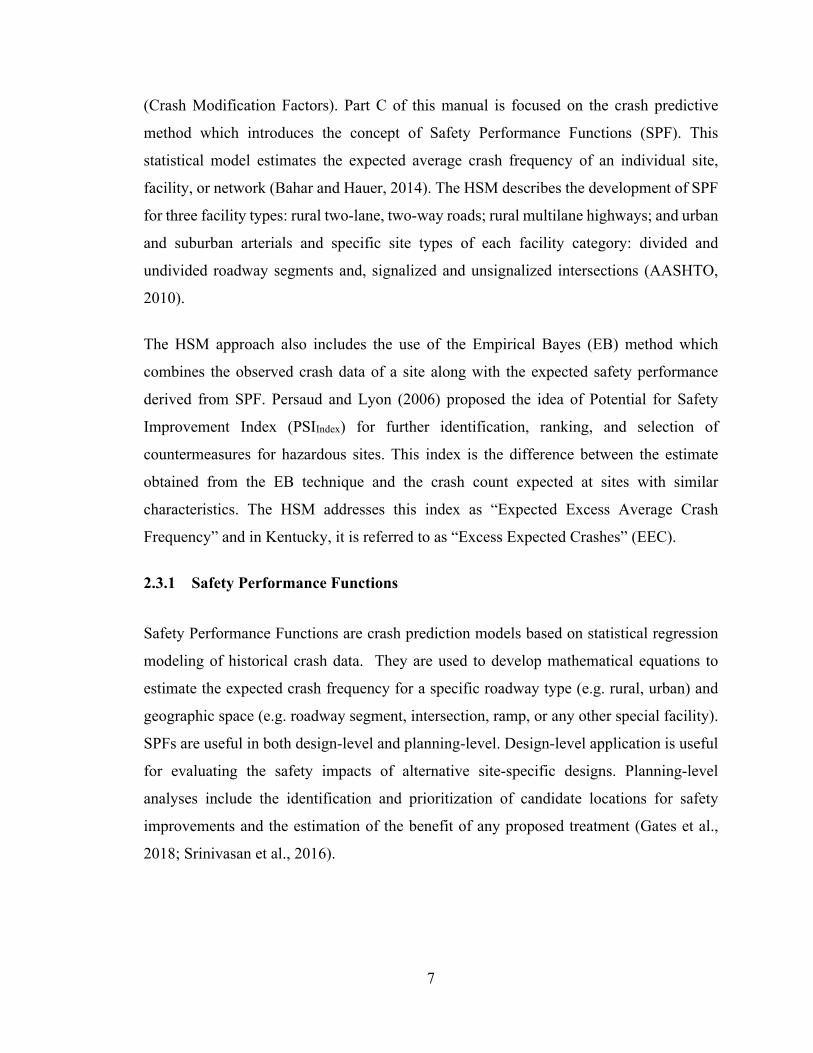
EEC is defined as the difference between EB expected crashes and SPF predicted crashes.
EEC quantifies the number of crashes occurring at a location more or less than what would
be expected (Blackden et al., 2018). The value of EEC can be both positive and negative.
Positive EEC represents that more crashes are occurring than expected at a site and
therefore, it has potential for improvements. A higher value indicates more vulnerability of
a site. On the other hand, negative EEC indicates that fewer crashes are occurring than
expected and so, those are comparatively safer sites. Figure 2-3 shows a visual
representation of the relationship between SPF predicted crashes, historic crashes, EB
expected crashes, and EEC.
Figure 2-3: Graphical representation of EEC
(-) EEC
(+) EEC

17
Chapter 3. METHODOLOGY
Chapter 2: Literature review delineated guidance on the HSM-based network screening
method by developing Safety Performance Functions and techniques to evaluate the
performance of potential models. This chapter will lay out the path this study will follow
to achieve the objectives. First of all, a brief description of the data and an overview of the
data preparation process is provided. The next section discusses the detailed process of
developing SPFs using the data along with a validation process. This is followed by several
statistical reliability assessments of the models. Finally, this chapter is concluded by
combining the observed crashes and SPF predicted crashes into EB estimate, followed by
the estimation of Excess Expected Crashes (EEC) for state-maintained rural two-lane roads
in Kentucky.
3.1 Data Preparation
Roadway data along with crash data are required for developing state-specific SPFs for any
facility type. For developing SPFs for Kentucky, the roadway geometric data and crash
data for all state-maintained rural two-lane roads have been collected. The following steps
have been followed to extract and prepare data for model development and further analysis.
3.1.1 Roadway Data
The roadway data for all state-maintained roads are available in the Roadway Centerline
Network and Highway Information System (HIS)3 database maintained by the Kentucky
Transportation Cabinet. The database contains information on traffic flow (TF), functional
classification (FS), and various roadway features (e.g. lanes, shoulders, vertical and
horizontal curves) in shapefile format. All of these shapefiles were combined into a
comprehensive database for all state-maintained roadway network in Kentucky. From the
3 https://transportation.ky.gov/Planning/Pages/Centerlines.aspx.

18
entire database, only rural two-lane data were extracted to another dataset which has been
used for developing and analyzing models for this study.
Segmentation is a vital process since the development and application of SPFs are
influenced by the organization of the dataset into distinct uniform units. Segmentation
enables the segregation of observed crashes within the bounds of a consistent mix of
roadway geometric features. A crash predictive model developed from the segments with
consistent geometric characteristics reflects the underlying pattern of the observed crashes
with more reliability and promise (Hariharan, 2015). Therefore, the rural two-lane dataset
was used to create statewide homogenous segmentation of roadways based on various
roadway features. Homogeneous segmentation is assured by fixed beginning and ending
mile points where traffic and road characteristics remain the same along the entire section.
The HSM provides guidance on which roadway attributes could be used to make the
segments homogeneous (AASHTO, 2010). The following features were used for this
segmentation:
• Average Annual Daily Traffic (AADT)
• Lane Width
• Shoulder Width
• Grade Class
• Curve Class
For rural two-lane roads, the segmentation process resulted in 277,437 uniform segments
covering around 20,000 miles of the rural two-lane road network. When multiple attributes
are used for segmentation, a lot of homogeneous segments get very short lengths. These
very short sections influence the crash rate resulting in unreliable crash prediction models
(Resende and Benekohal, 1997; Miaou, 1993). According to Hauer and Bamfo (1997), for
model development, road sections shorter than 0.1 miles should either be eliminated from
the dataset or reassembled to adjacent segments. In this study, removing such segments
would have taken away a significant number of segments which included almost half of
the total crashes of the dataset. On the other hand, aggregating shorter segments to adjacent
sections would hamper the homogeneity of the several segments. Miaou (1993) suggested

19
dropping road sections with lengths less than or equal to 0.05 miles. Therefore, the
minimum segment length was set to 0.05 miles. Moreover, any segment with zero AADT
is also removed from the database because this could also lead to bias. It was also made
sure that these segments did not include any intersection because the functional form and
required data for intersection’s SPF development are different from roadway sections.
Finally, the dataset was modified using the following three conditions.
• The minimum segment length was set to 0.05 miles.
• The AADT of any segment must be greater than zero.
• The section must not be an intersection or ramp.
Finally, 17,470 miles of rural two-lane roads were included in the database (divided into
143,554 segments). Table 3-1 presents the descriptive statistics of the explanatory variables
considered for model development and analysis.
Table 3-1: Description of the explanatory variables
Variables Unit Minimum Maximum Mean Standard Deviation
Most common attribute
AADT vehicles/day 2 19619 1223 1673 .
Segment Length miles 0.05 2.48 0.12 0.10 .
Lane Width feet 6 26 9.3 1.14 9
Shoulder Width feet 0 19 3.4 1.94 3
Grade Class4 Percentage 0-0.4
(Grade A) 8.5 or higher
(Grade F) - - B
Curve Class5 Degrees 0-3.4
(Curve A) 28 or higher (Curve F) - - A
4 Grade Class Description (Percentage): A=0-0.4; B=0.5-2.4; C=2.5-4.4; D=4.5-6.4; E=6.5-8.4; F=8.5 or higher 5 Curve Class Description (Degrees): A =0-3.4; B=3.5-5.4; C=5.5-8.4; D=8.5-13.9; E=14-27.9; F=28 or higher

20
3.1.2 Crash Data
The crash data were collected for five years (2013-2017) from the Kentucky State Police
(KSP) maintained database. The crashes (classified by severity using the KABCO scale6)
were linked to corresponding segments from the previous step. If a crash occurred between
the beginning and ending mile points of a segment, it was assigned to that segment. If a
crash occurred exactly at any start or endpoint, it was allocated to the segment with the
lower endpoint (Green, 2018). For this study, crashes of all severities were summarized
into total crashes. In total, 75,717 crashes had been linked to the 143,554 segments of rural
two-lane roads. Since the segments were quite small and crashes are rare and very random,
most of the segments (almost 70%) did not have any crashes.
3.1.3 Summary of the Final Dataset
The description of the key fields of the final dataset is summarized in Table 3-2.
Table 3-2: Description of the final dataset
Column Name Description
RT_UNIQUE
Route identifier in “WWW-XX-YYYYSS-ZZZ” format where:
WWW = County no. (e.g. 001 = Adair, 034 = Fayette)
XX = Route Prefix (e.g. KY = Kentucky, I = Interstate, CR = County road)
YYYY = Route Number
SS = Suffix (e.g. X=business, W=west, WX, west business
ZZZ = Cardinal/Noncardinal (e.g. 000 = cardinal, 010 = non-cardinal)
BEGIN_MP Beginning mile point
END_MP Ending mile point
6 K = Fatal crashes; A = Incapacitating injury; B = Non-incapacitating injury; C = Minor Injury; O = Property damage only (MMUCC, 3rd edition) K = Fatal injury; A = Suspected serious injury; B = Suspected minor injury; C = Possible injury; O = Property damage only (MMUCC, 4th edition definitions started in 2017).

21
LENGTH The difference between the ending and beginning mile points
LANEWID Lane width
SHLDWID Shoulder width
GRADECLS Vertical Curve
CURVECLS Horizontal Curve
CURVEDEG Degree of the horizontal curve
LASTCNT AADT
TOTAL Total crashes (fatal, injury crashes and property damage only)
3.2 Development of SPF
For the development of SPFs, the most widely used functional form has been used where
the segment length is used as a linear function and the traffic volume is considered to be
non-linear. The following equation has been used where a and b are regression parameters:
𝐒𝐒𝐒𝐒𝐒𝐒 𝐏𝐏𝐏𝐏𝐂𝐂𝐂𝐂𝐂𝐂 𝐏𝐏𝐂𝐂𝐏𝐏𝐏𝐏𝐞𝐞𝐂𝐂𝐏𝐏𝐏𝐏 = 𝑆𝑆𝛼𝛼 ∗ 𝐿𝐿𝑆𝑆𝑆𝑆𝑆𝑆𝑆𝑆ℎ ∗ 𝐴𝐴𝐴𝐴𝐶𝐶𝐴𝐴𝛽𝛽 𝐸𝐸𝐸𝐸. 12
Where,
α,β = Regression Parameters
Several statistical software tools such as SPSS, SAS, STATA, R, and LIMDEP can be used
to develop SPFs (Srinivasan and Bauer, 2013). Models can also be developed in Microsoft
Excel using solver or custom functions. To support the implementation of HSM predictive
techniques, the Federal Highway Administration (FHWA) has developed a software
program named the Interactive Highway Safety Design Model (IHSDM) and the National
Cooperative Highway Research Program (NCHRP) developed several spreadsheet tools
(AASHTO, 2010). Moreover, according to the CMF Clearinghouse website, thirteen states

22
have developed their state-specific SPFs and thirteen states have calibrated existing SPFs7
to their state-specific dataset. Several federal agencies have modified, expanded or
recreated the tools for developing SPFs through automation, or additional features:
Kentucky Transportation Cabinet (SPF-R), Ohio DOT (Economic Crash Analysis Tool),
Illinois DOT (HSM Crash Prediction Tool), Michigan DOT (Part C Spreadsheet) to name
a few.
In this study, “SPF-R”, a script in RStudio developed by the Kentucky Transportation
Center (KTC) has been used for SPF development. This tool estimates Negative Binomial
regression models using generalized linear modeling techniques. The open-source
automation tool is available on GitHub at http://github.com/irkgreen/SPF-R. Though
several tools can generate SPF manually, developing models is complicated and laborious
since it requires several iterations and filtering of the roadway dataset. This script is
considered to be more efficient with instant feedbacks and it is customizable to a variety
of potential uses (Blackden et al., 2018). As an input, the code requires a CSV-format file
with a specific set of attributes of roadway segments, intersections, or ramps. Since this
study dealt with segments only, the required attributes were the length of the homogeneous
segments, crashes, and traffic volume of each segment. The SPF-R tool itself must be
configured for a specific project with its own paths for input and output, as well as any
additional model specifications. An excel file with model parameters and goodness-of-fit
measures, a Cumulative Residual (CURE) plot, a scatter plot, and four box plots (length,
crashes, crashes per mile, and AADT) are the outputs of the tool.
3.2.1 Cross-Validation
Cross-validation is one of the most widely used techniques to estimate the accuracy of the
performance of a predictive model. There are several methods for performing cross-
validation, e.g. train-test split approach, K-folds cross-validation, etc. In this study, the
train-test split method has been used for evaluating the performance of the models. This
approach is based on splitting the dataset into two parts: the training set and the testing set.
The training set is the one that is used to develop models and explore relationships among
7 http://www.cmfclearinghouse.org/resources_spf.cfm
23
the explanatory variables and the response. The rest of the data is called the testing set
which is used to measure the performance of the fitted models (Kuhn and Johnson, 2019).
The size of each of the sets is random but in general, the training set is bigger than the
testing set. Ideally, the data is split into 70:30, 75:25, or 80:20 ratio (Varoquaux, 2018;
Kuhn and Johnson, 2019). This approach might not be suitable if the dataset has limited
data because some important records could be eliminated from the training dataset resulting
in a high bias. The dataset used for this study is large enough to get similar distribution in
training and testing sets. Therefore, 75% of the data was assigned to the training set using
a random number generating function, and the rest was used as the testing set. The
descriptions of the training and testing datasets are shown in Table 3-3.
Table 3-3: Description of the train-test datasets
Dataset Total segments Total length (miles) Total crashes
Training Dataset (75%) 106,922 13,061 56,516
Testing Dataset (25%) 36,632 4,409 19,201
3.2.2 Attributes used for SPF Development
In this study, 15 SPFs have been developed. The attributes used for those model
development process are described below:
3.2.2.1 Generic SPF
The first SPF was developed using the entire training dataset. This is the most generic
model which included segments with all the attributes of interest (lane width, shoulder
width, curve class, and grade class) and none of them was specified to any particular value.
In this study, this model will be referred to as the “generic model”. The “generic” model
would have omitted variable bias because the variable/s that might contribute to crash

24
prediction were not included in the model. This can also lead to overfitting of the model
and modeling noise.
3.2.2.2 SPF with Specific Attributes
Developing a more reliable SPF required filtering the dataset with various base conditions.
But the application of filters reduces the sample size. Depending on the extent of the filters,
sometimes the dataset becomes too small to execute a model (Green, 2018). According to
Srinivasan et. al (2013), the minimum sample would be 100-200 miles with at least 300
crashes per year. When a dataset for a specific set of attributes met these criteria, an SPF
was developed from that dataset. Multiple iterations were performed with various sets of
base conditions. Among the models, the most reliable SPF was chosen based on goodness-
of-fit measures. This model will be referred to as the “specific” model in this study. The
base conditions used for this model are given below:
o Lane Width = 9 feet
o Shoulder Width = 3 feet
o Curve Class = A
o Grade Class = A
3.2.2.3 SPF with Ranges of Attributes
Though reliable SPFs can be developed, in absence of appropriate AFs, they cannot be
used in the subsequent steps of network screening e.g. adjusting predicted crashes,
estimating EB crashes, and, ultimately estimation of EEC. One of the goals of this study
was to reduce the necessity of AFs as much as possible. Therefore, instead of using one
specific value for a variable, a series of models have been developed using a range of values
for that same variable. It was made sure that every range included the specific value of an
attribute that was used to develop the “specific” model and the ranges were expanded
around that value. For example, one model was developed including all roads between 7
feet to 11 feet lanes instead of using all 9 feet lanes only. This way, more segments, as well
as model miles were included in the SPFs and there were fewer segments to adjust. In total,

25
13 SPFs were developed using various ranges of attributes. Table 3-4 summarizes the base
conditions used to develop those SPFs.
Table 3-4: Ranges used to develop 13 SPFs
Model
Base Conditions
Lane
Width
Shoulder
Width Grade Curve
1 9-13 3-6 A A
2 9 0-3 A, B A
3 9 3-6 A, B A, B
4 9-10 0-3 A, B A, B
5 8-10 0-6 A, B A, B
6 8-10 2-4 A, B A, B
7 7-11 0-6 A, B A, B
8 9 3 A, B, C A
9 9-13 0-3 A A, B, C
10 9-13 3 A A, B
11 7-11 2-4 A, B A, B
12 7-13 0-6 A, B A, B
13 7-13 0-6 A, B, C A, B, C
3.2.3 Goodness-of-Fit Measures
Goodness-of-Fit (GOF) measures evaluate the reliability of a prediction model by
quantifying how well it fits the observed data. It is important to check the reliability of a
regression model because it helps to identify potential issues of the model and ways to

26
improve it. These measures can also be used to compare the performance of multiple
models and make the best choice. Some GOF measures can be used by directly comparing
the relative performances of the contending SPFs by following the existing guidelines. On
the other hand, some measures need the subjective judgment of the visual representations
since there are no acceptable thresholds (Lyon et al., 2016). In the study of SPF
development, one of the most important GOF matrices is CURE plots. It is a reflection of
the functional form of the particular explanatory variable, in this case, AADT. A CURE
plot derived from a reliable SPF should have the following qualities.
• The plot is expected to oscillate around X-axis.
• The cumulative residuals are expected to stay within two standard deviations.
• It should be free of outliers (large vertical jumps).
• It should have minimum upward or downward drifting.
There are several other GOF measures to assess the performance of SPFs. Apart from
CURE plots, Table 3-5 summarizes all the GOF measures used to evaluate the SPFs for
this study.
Table 3-5: Summary of GOF measures for SPFs
GOF Measures Preferred values
Modified R2 Higher values
Cure Deviation Percentage (CDP) Lower values (Less than 5%)
Theta (Inverse Overdispersion) Higher values
Maximum Absolute CURE Deviation
(MACD) Lower values
Root Mean Square Error (RMSE) Lower Values

27
3.3 Validation using Testing Dataset
Where the 75% data of the whole dataset was used to develop the SPFs, 25% of them were
used to validate the models. There are several statistical metrics e.g. Mean Absolute
Percent Error (MAPE), Mean Square Error (MSE), Root Mean Square Error (RMSE)
which can be used to measure the predictive capacity of a model. All of these measures
calculate error by taking the difference between observed and predicted crashes of a
segment. MAPE takes the absolute value of the error term as a percentage of the observed
crashes. Since the observed crashes are at the denominator, MAPE cannot be calculated
for the segments with zero crashes (Hariharan, 2015). In this study, around 70% of the
segments do not have any crashes. Therefore, MAPE would not be an appropriate
validation metric.
MSE is the average of the squared error term and RMSE is the square root of MSE. Since
both of these measures indicate similar interpretations, RMSE is chosen as the validation
metric for this study. When calculating the RMSE for each model on the testing data, the
dataset was filtered using the attributes used for developing that particular SPF. The RMSE
is calculated in two days:
• RMSE1: In this case, the errors were calculated by comparing the predicted crashes
to the observed crashes. Due to the randomness of crash data, it possesses
regression-to-the-mean bias which might affect the RMSE.
• RMSE2: In this case, the errors were by comparing the predicted crashes to the EB
estimate which is a function of the observed crashes. EB method accounts for the
regression-to-the-mean bias by dragging the crash counts to the mean (Hauer et al.,
2002).
3.4 Adjustment of SPF Predicted Crashes using Adjustment Factors
Apart from narrowing down the sample size, the application of filters introduces the need
for adjustment factors (AFs). AFs are required when any segment’s geometric attributes
are different from the model’s base conditions. AFs are multiplicative factors and equation
is for adjusting the model predicted crashes is shown below:

28
𝐀𝐀𝐏𝐏𝐀𝐀𝐀𝐀𝐂𝐂𝐏𝐏𝐏𝐏𝐏𝐏 𝐒𝐒𝐒𝐒𝐒𝐒 𝐂𝐂𝐏𝐏𝐂𝐂𝐂𝐂𝐂𝐂𝐏𝐏𝐂𝐂 = 𝑆𝑆𝑆𝑆𝐶𝐶 𝐶𝐶𝐼𝐼𝑉𝑉𝐼𝐼ℎ𝑆𝑆𝐼𝐼 (𝑏𝑏𝑉𝑉𝐼𝐼𝑆𝑆 𝐼𝐼𝐼𝐼𝑆𝑆𝑐𝑐𝐼𝐼𝑆𝑆𝐼𝐼𝐼𝐼𝑆𝑆) ∗ 𝐴𝐴𝐶𝐶𝐿𝐿𝐿𝐿 ∗ 𝐴𝐴𝐶𝐶𝑆𝑆𝐿𝐿 ∗ 𝐴𝐴𝐶𝐶𝐶𝐶𝐶𝐶 ∗ 𝐴𝐴𝐶𝐶𝐺𝐺𝐺𝐺
…Eq. 13
For rural two-lane roads, the adjustment factors for lane width and vertical curve are
obtained from the HSM (AASHTO, 2010) and those for shoulder width are obtained from
the CMF Clearinghouse. The adjustment factors for lane width, shoulder width, and
vertical curve are described in Table 3-6, Table 3-7, and Table 3-8 respectively.
Table 3-6: Adjustment factors for lane width (rural two-lane)
Lane Width (ft)
AF
AADT <400 AADT (400-2000) AADT>2000
9 or less (base) 1 1 1
10 0.97
1.02+.000175*(AADT-400)/ 1.05+.000281*(AADT-400) Or, 0.622776+(1302.8/(AADT+3336.65))
0.87
11 0.96
1.01+.000025*(AADT-400)/ 1.05+.000281*(AADT-400) Or, 0.088968+(3261.86/(AADT+3336.65))
0.7
12 or more 0.95 1/(1.05+.000281*(AADT-400)) Or, 3558.72/(AADT+3336.65)
0.67
Table 3-7: Adjustment factors for shoulder width (rural two-lane) [Source: CMF Clearinghouse8]
Shoulder Width
(ft) AF
0 1.145
1 1.12
2 1.03
3 1
8 http://www.cmfclearinghouse.org/study_detail.cfm?stid=338

29
4 0.975
5 0.945
6 0.93
7 0.905
8 0.875
Table 3-8: Adjustment factors for vertical curves (rural two-lane)
Vertical Curve Grade AF
0-3% 1
3-6% 1.1
>6% 1.16
The HSM provides a function for estimating AFs for horizontal curves of rural two-lane
highways. According to (Wu et al., 2017), the HSM function is not very effective because
it was developed based on outdated data and analysis techniques. This study developed an
equation to calculate the adjustment factor for horizontal curves and this function is also
recommended by the CMF Clearinghouse9. The equation is as follows:
𝐴𝐴𝐶𝐶 = 196.4 ∗ 𝐶𝐶𝑉𝑉𝑐𝑐𝐼𝐼𝑅𝑅𝐼𝐼−0.65 𝐸𝐸𝐸𝐸. 14
3.5 EB Estimates and Calculation of EEC
In the previous section, in total 15 SPFs were developed: one generic SPF, one with specific
values of each attribute (referred to as the “specific” model), and 13 SPFs with ranges of
values of each attribute. The regression parameters obtained from each model are used to
estimate the SPF crashes for every segment of the entire dataset and the predicted crashes
were adjusted using appropriate adjustment factors (described in section 3.3).
The safety of a site is best estimated when both the number of observed crashes and the
number of crashes predicted by the SPF of that site are combined. Empirical Bayes Method
9 http://www.cmfclearinghouse.org/study_detail.cfm?stid=481

30
estimates the expected crashes using a mathematical combination of the observed and
predicted crash frequencies. Equations 14 and 15 were used to calculate the EB estimates
for each segment.
𝐄𝐄𝐄𝐄 𝐄𝐄𝐄𝐄𝐄𝐄𝐏𝐏𝐏𝐏𝐏𝐏𝐏𝐏𝐏𝐏 𝐂𝐂𝐏𝐏𝐂𝐂𝐂𝐂𝐂𝐂𝐏𝐏𝐂𝐂 =
𝑤𝑤𝑆𝑆𝐼𝐼𝑆𝑆ℎ𝑆𝑆 ∗ 𝑆𝑆𝑆𝑆𝐶𝐶 𝑝𝑝𝐼𝐼𝑆𝑆𝑐𝑐𝐼𝐼𝐼𝐼𝑆𝑆𝑆𝑆𝑐𝑐 𝐼𝐼𝐼𝐼𝑉𝑉𝐼𝐼ℎ𝑆𝑆𝐼𝐼 + (1 − 𝑤𝑤𝑆𝑆𝐼𝐼𝑆𝑆ℎ𝑆𝑆) ∗ 𝐼𝐼𝑏𝑏𝐼𝐼𝑆𝑆𝐼𝐼𝑜𝑜𝑆𝑆𝑐𝑐 𝐼𝐼𝑆𝑆 𝑆𝑆ℎ𝑉𝑉𝑆𝑆 𝐼𝐼𝐼𝐼𝑆𝑆𝑆𝑆 𝐸𝐸𝐸𝐸. 14
𝒘𝒘𝒘𝒘𝒘𝒘𝒘𝒘𝒘𝒘𝒘𝒘 = 1
1 +
𝑆𝑆𝑆𝑆𝐶𝐶 𝐶𝐶𝐼𝐼𝑉𝑉𝐼𝐼ℎ𝑆𝑆𝐼𝐼𝑆𝑆𝑆𝑆𝑆𝑆𝑆𝑆𝑆𝑆𝑆𝑆𝑆𝑆 𝐿𝐿𝑆𝑆𝑆𝑆𝑆𝑆𝑆𝑆ℎ
𝜃𝜃
𝐸𝐸𝐸𝐸. 15
Where,
𝜭𝜭 = Inverse overdispersion parameter
Since crashes are random in nature, they are not normally distributed and they exhibit over-
dispersion with a variance higher than the mean. Therefore, the traditional standard
deviation formula used for normally distributed data would not reflect the correlation
properly. The standard deviation (σ) of the EB estimate is calculated by:
𝜎𝜎 = �(1 − 𝑤𝑤𝑆𝑆𝐼𝐼𝑆𝑆ℎ𝑆𝑆) ∗ 𝐸𝐸𝐸𝐸 𝐸𝐸𝐼𝐼𝑆𝑆𝐼𝐼𝑆𝑆𝑉𝑉𝑆𝑆𝑆𝑆 𝐸𝐸𝐸𝐸. 16
Excess Expected Crashes (EEC) for each segment was calculated using the crashes
predicted by SPF and the crashes adjusted by Empirical Bayes (EB) method. Equation 16
was used to calculate the EEC.
𝐄𝐄𝐄𝐄𝐂𝐂 = 𝐸𝐸𝐸𝐸 𝐸𝐸𝐼𝐼𝑆𝑆𝐼𝐼𝑆𝑆𝑉𝑉𝑆𝑆𝑆𝑆𝑐𝑐 𝐶𝐶𝐼𝐼𝑉𝑉𝐼𝐼ℎ𝑆𝑆𝐼𝐼 − 𝑆𝑆𝑆𝑆𝐶𝐶 𝑆𝑆𝐼𝐼𝑆𝑆𝑐𝑐𝐼𝐼𝐼𝐼𝑆𝑆𝑆𝑆𝑐𝑐 𝐶𝐶𝐼𝐼𝑉𝑉𝐼𝐼ℎ𝑆𝑆𝐼𝐼 𝐸𝐸𝐸𝐸. 17
3.6 Comparison of Segment Ranking
The EEC depicts how much potential a site, in this case, a segment has for improvement.
The segments with positive EEC indicate their need for improvement and the segments
with negative EEC are at a comparatively lower risk. The EEC of each segment varies
depending on the SPF used. 15 SPFs were used individually to calculate each segment’s
EEC. These segments were prioritized by their EEC value. The entire dataset was sorted

31
in descending order where the top segments have the most potential for safety
improvements.
The ranking of the segments estimated by each of the 15 models was compared among
themselves using Spearman’s rank correlation coefficient. This coefficient is used to
measure the rank correlation between the rankings of a variable (i.e. EEC) estimated by
two different models. The values vary between -1 and 1. The Spearman correlation will be
high when two models produce a similar rank (correlation will be 1 if the rank is identical).

32
Chapter 4. RESULTS AND ANALYSIS
An automation tool, SPF-R has been used to develop 15 SPFs from the training dataset
with various combinations of geometric attributes and the testing dataset was used to
validate them. The tool provided a CURE plot, scatter plot, and an excel document with
regression parameters, goodness-of-fit measures, and other details for each model. In this
section, CURE plots, GOF metrics (e.g. Modified R2, CDP, MACD, theta), and predictive
metric (e.g RMSE) were used to evaluate the SPFs and to determine which SPF will work
the best. Going forward, this chapter also compares the ranking of the segments executed
by each model.
4.1 Model Output
In this study, the sample sizes of the models varied significantly because of the variation
in base geometric conditions. Table 4-1 summarizes the total length covered, and the total
number of crashes for each model.
Table 4-1: Description of the sample used for SPF development
Model Total Length (miles)
Total Crashes
Generic 13061 56516 Specific 126 457
1 600 3935 2 457 1660 3 507 1920 4 1049 5299 5 1650 8653 6 1522 7872 7 1950 11288 8 407 1359 9 492 2933 10 327 2006 11 1744 9770 12 2025 12529 13 2889 17422

33
4.1.1 Model Parameters
The regressions parameters of the SPFs are the output from Negative Binomial regression.
The value of α ranged between -5.481 and -4.135 and, the value of β varied between 0.80
and 0.98. The inverse overdispersion parameter is also estimated along with the
coefficients of the regression parameters. The degree by which the variance in the crash
data is exceeded by mean is represented by the overdispersion parameter. SPF-R reports
this parameter as theta which is the reciprocal of the overdispersion parameter. The value
of theta varied between 1.157 and 2.615. The regression coefficients and theta for the SPFs
are presented in Table 4-2.
Table 4-2: Regression parameters and inverse overdispersion parameter
Model α β Theta
Generic -4.135 0.802 1.157 Specific -4.661 0.855 2.392
1 -4.836 0.882 1.798 2 -5.167 0.926 2.163
3 -4.987 0.898 2.209 4 -5.314 0.949 1.908 5 -4.966 0.902 1.909 6 -4.982 0.903 2.115 7 -4.799 0.876 1.964 8 -5.167 0.916 2.615 9 -5.481 0.980 1.503 10 -5.336 0.961 1.557
11 -4.906 0.891 2.100 12 -4.976 0.901 1.621 13 -4.832 0.885 1.526

34
4.1.2 CURE Plots
CURE plots are the visual representation of the model form and it helps to detect omitted
variable bias and outliers. In each CURE plot, the blue and green lines represent the upper
and lower confidence bands respectively and the red dots indicate the cumulative residuals.
The “generic” SPF was developed from the whole training dataset. The resulting CURE
plot (Figure 4-1) of the “generic” SPF has a clear downward drift which is an indication
of omitted variable bias. For a reliable model, the cumulative residuals are expected to
oscillate within the confidence band. But for this model, 85% of data have transgressed
from the bands. The model also has low modified R2 value and theta and high MACD
(Table 4-3). The CURE plot along with the other GOF measures indicates that the generic
model is quite unreliable.
Figure 4-1: CURE plot of “generic” SPF
Table 4-3: GOF measures of the “generic” SPF
GOF Metric Value
R2 0.25
CDP 85%
MACD 4192.8
Theta 1.157
The CURE plot of the “specific” model is shown in Figure 4-2 and the GOF metrics are
provided in Table 4-4. The CURE plot of this model is quite satisfactory since it oscillates
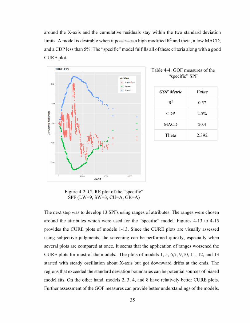
35
around the X-axis and the cumulative residuals stay within the two standard deviation
limits. A model is desirable when it possesses a high modified R2 and theta, a low MACD,
and a CDP less than 5%. The “specific” model fulfills all of these criteria along with a good
CURE plot.
Figure 4-2: CURE plot of the “specific” SPF (LW=9, SW=3, CU=A, GR=A)
Table 4-4: GOF measures of the “specific” SPF
GOF Metric Value
R2 0.57
CDP 2.5%
MACD 20.4
Theta 2.392
The next step was to develop 13 SPFs using ranges of attributes. The ranges were chosen
around the attributes which were used for the “specific” model. Figures 4-13 to 4-15
provides the CURE plots of models 1-13. Since the CURE plots are visually assessed
using subjective judgments, the screening can be performed quickly, especially when
several plots are compared at once. It seems that the application of ranges worsened the
CURE plots for most of the models. The plots of models 1, 5, 6,7, 9,10, 11, 12, and 13
started with steady oscillation about X-axis but got downward drifts at the ends. The
regions that exceeded the standard deviation boundaries can be potential sources of biased
model fits. On the other hand, models 2, 3, 4, and 8 have relatively better CURE plots.
Further assessment of the GOF measures can provide better understandings of the models.
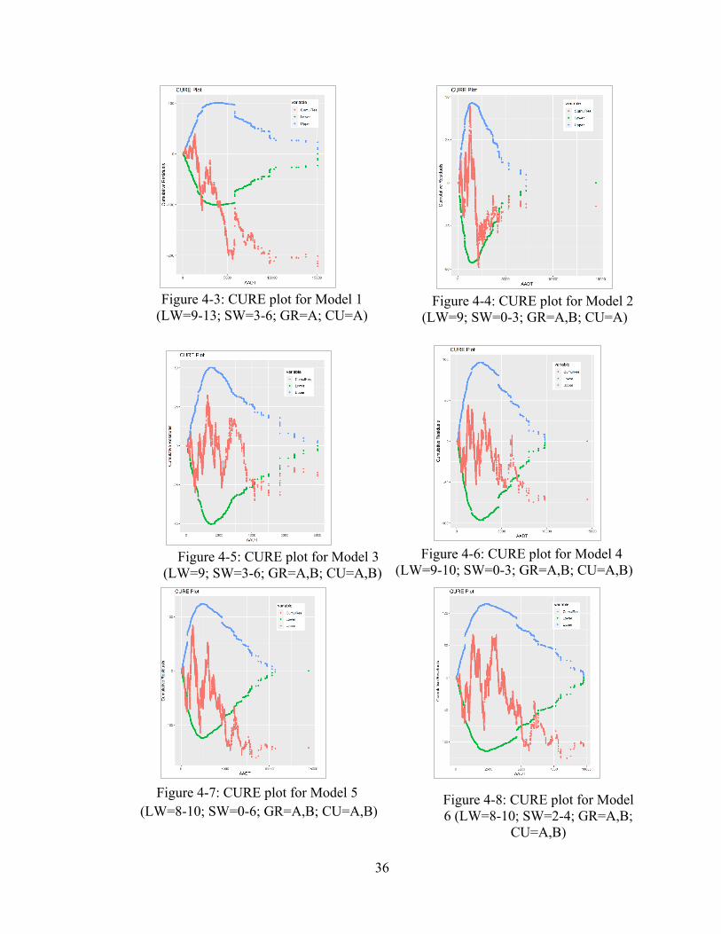
36
Figure 4-3: CURE plot for Model 1
(LW=9-13; SW=3-6; GR=A; CU=A)
Figure 4-4: CURE plot for Model 2
(LW=9; SW=0-3; GR=A,B; CU=A)
Figure 4-5: CURE plot for Model 3
(LW=9; SW=3-6; GR=A,B; CU=A,B)
Figure 4-6: CURE plot for Model 4
(LW=9-10; SW=0-3; GR=A,B; CU=A,B)
Figure 4-7: CURE plot for Model 5
(LW=8-10; SW=0-6; GR=A,B; CU=A,B)
Figure 4-8: CURE plot for Model 6 (LW=8-10; SW=2-4; GR=A,B;
CU=A,B)

37
Figure 4-9: CURE plot for Model 7
(LW=7-11; SW=0-6; GR=A,B; CU=A,B)
Figure 4-10: CURE plot for Model 8 (LW=9; SW=3; GR=A,B,C; CU=A)
Figure 4-11: CURE plot for Model 9
(LW=9-13; SW=0-3; GR=A; CU=A,B,C)
Figure 4-12: CURE plot for Model 10
(LW=9-13; SW=3; GR=A; CU=A,B)
Figure 4-13: CURE plot for Model 11
(LW=7-11; SW=2-4; GR=A,B; CU=A,B)
Figure 4-14: CURE plot for Model 12
(LW=7-13; SW=0-6; GR=A,B; CU=A,B)

38
Figure 4-15: CURE plot for Model 13 (LW=7-13; SW=0-6; GR=A,B,C;
CU=A,B,C)
4.1.3 Comparison of Goodness-of-Fit Measures
Along with CURE plots, goodness-of-fit measures are also important when multiple
models are compared. This section compares the GOF measures of all SPFs to evaluate
their performances. AIC and BIC were not included here because these parameters are
better suited when comparing models with a constant sample size (Green, 2018) and this
study evaluates models with varying sample sizes. The values of every metric are plotted
in individual bar charts to show the relative comparison among the models. In every graph,
the red bar indicates the values for the “generic” model and the green bar represents that
for the “specific” model.
• Modified R2
The R2 value of an SPF measures the potentially explainable variation of the model.
The R2 values used in this study are refined since Negative Binomial regression does
not estimate any metric that is equivalent to R2 (Green, 2018). Higher values are
preferable for this metric. The generic model has the lowest modified R2 value which
is 0.25. Modified R2 improves when attributes are specified for the SPFs. Only one SPF
(model 8) has a higher modified R2 than the “specific” model. The comparison of
modified R2 values is shown in Figure 4-16.

39
Figure 4-16: Comparison of modified R2
• CURE Deviation Percentage (CDP)
CDP represents the percentage of data that transgress outside the two standard
deviation boundaries of any SPF’s CURE plot. Values under 5% are optimal at the 95%
confidence level. The “generic” model had the poorest CURE plot with 85% of data
outside the confidence bands where the “specific” model had the best CURE plot with
only 2.5% transgressed data.
The CDP value for the other 13 models varied between 2.5% and 85%. Apart from
model 4, all the models had CDP greater than 5%. Nonetheless, models 2, 3, and 8 can
be considered as potential models along with model 4 with their relatively lower CDP
values. Figure 4-17 represents the comparison of CDP values.
0.570.33
0.570.51
0.430.41
0.450.41
0.580.35
0.340.43
0.320.31
0.25
0.00 0.10 0.20 0.30 0.40 0.50 0.60 0.70
Specific123456789
10111213
Generic
Modified R2
Mod
el
Comparison of modified R2

40
Figure 4-17: Comparison of CDP
• Maximum Absolute CURE deviation (MACD)
MACD measures the largest absolute cumulative residual in a CURE plot and smaller
values are optimal. Coherent to the CURE plots and CDP values, the “generic” model
has the highest MACD. From Figure 4-18, it is seen that all models have a larger
absolute deviation compared to the “specific” model. However, models 2, 3, and 8 can
be considered as desirable candidates based on the lower ranges of MACD values.
2.516.1
5.47.7
4.018.1
17.018.4
8.210.1
13.316.0
19.523.3
85.0
0.0 5.0 10.0 15.0 20.0 25.0 30.0 35.0 40.0
Specific
2
4
6
8
10
12
Generic
CDP (%)
Mod
el
Comparison of CDP
90.0
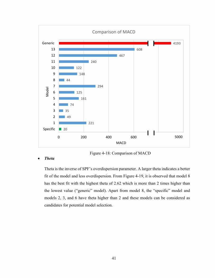
41
Figure 4-18: Comparison of MACD • Theta
Theta is the inverse of SPF’s overdispersion parameter. A larger theta indicates a better
fit of the model and less overdispersion. From Figure 4-19, it is observed that model 8
has the best fit with the highest theta of 2.62 which is more than 2 times higher than
the lowest value (“generic” model). Apart from model 8, the “specific” model and
models 2, 3, and 6 have theta higher than 2 and these models can be considered as
candidates for potential model selection.
20
221
49
35
74
161
125
294
44
148
122
240
467
608
4193
0 200 400 600 800 1000
Specific
1
2
3
4
5
6
7
8
9
10
11
12
13
Generic
MACD
Mod
el
Comparison of MACD
5000

42
Figure 4-19: Comparison of theta
4.2 Cross-validation
The entire dataset of rural two-lane roads was divided into training and testing datasets to
perform cross-validation. 75% of the were taken as the training data to develop SPFs and
the above-mentioned GOF measures are obtained from the models. In this section, the
models are validated using the 25% testing dataset. The metric used for the validation
process is Root Mean Square Error (RMSE). RMSE is calculated by taking the average of
the square of the error at each segment. Before calculating the RMSE for each model, the
dataset was filtered using the same base conditions used to develop that particular model
so that the model development and the validation dataset have the same geometric
characteristics. As mentioned in section 3.3, the RMSE is calculated in two ways: by
comparing observed and predicted crashes (RMSE1), and by comparing EB estimates and
predicted crashes (RMSE2). The resulting RMSE values are presented in Table 4-5 and
Table 4-6 respectively.
2.391.80
2.162.21
1.911.91
2.111.96
2.621.50
1.562.10
1.621.53
1.16
0.00 0.50 1.00 1.50 2.00 2.50 3.00
Specific123456789
10111213
Generic
Theta
Mod
el
Comparison of theta

43
It is desirable to obtain as low value as possible for a predictive measure based on any error
term (Hariharan, 2015). But, both the tables show that the overall RMSE values are quite
high and most of them are above or closer to one. Since RMSE was estimated by squaring
the error term, segments with large differences between predicted and observed or,
predicted and EB estimate were weighted disproportionately in comparison to other
segments that resulted in higher RMSE. For every model, RMSE2 is lower than RMSE1.
This is because RMSE2 uses EB estimate which accounts for the regression-to-the-mean
bias present in the observed crashes.
Among the 15 models, model 8 has the lowest RMSE1 and RMSE2 which indicates that
model 8 has the best predictive ability which is even significantly better than the “specific”
model.
Table 4-5: RMSE (Comparing predicted crashes with observed crashes)
Model RMSE1
Generic 1.27 Specific 0.94
1 2.52 2 0.80 3 0.94 4 0.91 5 1.00 6 1.09 7 1.17 8 0.73 9 2.27 10 2.86 11 1.15 12 1.88 13 1.69
Table 4-6: RMSE (Comparing predicted crashes with EB estimates)
Model RMSE2
Generic 1.13 Specific 0.62
1 2.20 2 0.55 3 0.70 4 0.69 5 0.78 6 0.83 7 0.94 8 0.46 9 2.05 10 2.60 11 0.92 12 1.67 13 1.49

44
4.3 Choosing the Best Model
A desirable model should possess high modified R2 and theta, low MACD and RMSE, and
CDP under 5%. The application of ranges of variables showed improvement compared to
the “specific” model in several GOF metrics. Based on the results shown in Sections 5.1.3
and 5.2, five SPFs (the “specific” model and models 2, 3, 4, and 8) are chosen to be
considered for the final assessment of the model selection process. The GOF metrics and
predictive measures of these five SPFs are summarized in Table 4-7 where darker cells
represent more optimal values.
Table 4-7: GOF and predictive measures of the final five models
Model
Base Conditions Training Data Testing Data
LW SW GR CU Mod R2
CDP (%) MACD 𝜭𝜭 RMSE1 RMSE2
Specific 9 3 A A 0.57 2.5 20 2.39 0.94 0.62
2 9-13 3-6 A A 0.57 5.4 49 2.16 0.8 0.55
3 9 3-6 A,B A,B 0.51 7.7 35 2.21 0.94 0.7
4 9-10 0-3 A,B A,B 0.43 4 74 1.91 0.91 0.69
8 9 3 A,B,C A 0.58 8.2 44 2.62 0.73 0.45
The table above indicates that model 8 has got the optimal Modified R2, theta, RMSE1, and
RMSE2 values. It also has a comparatively lower MACD value. Though the CDP value is
not under a 5% significance level, it can still be accepted considering the quality of the
CURE plot. Therefore, model 8 which was developed using 9 feet lanes, 3 feet shoulders,
A, B, and C grade horizontal curves and A grade vertical curve is chosen to be the new
best model replacing the specific model.

45
4.4 Ranking Segments with Excess Expected Crashes (EEC)
Every segment of the entire dataset was used to calculate the EEC values for all 15 models.
Nearly 24% of the segments have positive EEC which indicates more crashes are occurring
than expected in those segments. The descriptive statistics of the EEC are shown in Table
4-8. The maximum values of EEC ranged between 62.3 (model 8) and 71.7 (“generic”
model).
Table 4-8: Descriptive statistics of EEC for 15 SPFs
Model Mean EEC
Minimum EEC
Maximum EEC
Generic -0.034 -23.6 71.7
Specific -0.010 -11.3 63.1
1 -0.103 -20.7 69.2
2 -0.020 -13.4 65.3
3 0.005 -12.2 64.5
4 -0.005 -19.2 65.8
5 -0.028 -16.5 66.4
6 -0.024 -14.3 65.4
7 -0.035 -14.5 65.7
8 0.009 -11.6 62.3
9 -0.098 -29.7 70.9
10 -0.131 -28.4 70.7
11 -0.036 -13.6 65.2
12 -0.079 -21.9 69.9
13 -0.054 -21.8 70.3

46
4.4.1 Comparison of Rank of the Segments
After applying all the models on the whole dataset for EEC calculation, it was sorted in
descending order where the top segments have the most potential for safety improvements.
Each segment is assigned with a rank and the ranking obtained by the models are compared
to each other using Spearman’s rank correlation coefficient. The metrics are summarized
in Table 4-9. The value of this coefficient gets higher when ranking estimated by any two
models are similar. It is seen that the values of Spearman’s coefficient are significantly
high (mostly closer to 1) for any pair of SPFs. That means no matter what model is used,
the screening process provides an almost identical ranking of the segments.

47
Table 4-9: Spearman's Rank Correlation Matrix
Generic Mod 1
Mod 2
Mod 3
Mod 4
Mod 5
Mod 6
Mod 7
Mod 8
Mod 9
Mod 10
Mod 11
Mod 12
Mod 13
Specific
Generic 1
Mod 1 0.89 1
Mod 2 0.87 0.97 1
Mod 3 0.86 0.95 0.98 1
Mod 4 0.88 0.95 0.98 0.99 1
Mod 5 0.87 0.96 0.98 0.99 0.99 1
Mod 6 0.87 0.96 0.98 0.99 0.99 1.00 1
Mod 7 0.87 0.96 0.97 0.99 0.98 0.99 0.99 1
Mod 8 0.86 0.96 0.99 0.98 0.97 0.97 0.97 0.97 1
Mod 9 0.92 0.95 0.92 0.92 0.93 0.93 0.93 0.93 0.90 1
Mod 10 0.89 0.97 0.94 0.94 0.95 0.96 0.96 0.96 0.93 0.97 1
Mod 11 0.88 0.96 0.97 0.99 0.98 0.99 0.99 1.00 0.96 0.94 0.97 1
Mod 12 0.90 0.98 0.96 0.97 0.97 0.98 0.97 0.98 0.95 0.96 0.99 0.98 1
Mod 13 0.92 0.95 0.94 0.94 0.95 0.95 0.95 0.95 0.93 0.99 0.96 0.95 0.97 1
Specific 0.85 0.96 0.99 0.98 0.97 0.97 0.97 0.97 1.00 0.90 0.93 0.97 0.95 0.92 1
47

48
4.4.2 Comparison of the EEC Values for Top 10 Rural Two-lane Segments
After the ranks of the segments were obtained, the top 10 rural two-lane segments for each
model are taken to compare the values of EEC. The top 10 segments provided by all 15
models are identical (only for the “Generic” model, segments with rank 3 and 4 swapped
places). The route ID, beginning, and ending mile points of the segments are provided in
Table 4-10. The EEC values of these segments are plotted for relative comparison. For
better illustration, segments are divided into two groups: segments with rank 1-5 are shown
in Figure 4-20, and segments with rank 6-10 are shown in Figure 4-21. For a particular
segment’s rank, there are 15 bars which represent the EECs calculated by each of the 15
SPFs.
Table 4-10: Ranking of the top 10 segments
Rank Route ID Beginning Milepoint
Ending Milepoint
1 030-US-0431 -000 1.52 1.66
2 030-US-0431 -000 1.025 1.25
3* 049-US-0027 -000 5.08 5.97
4* 005-US-0068 -000 1.42 1.87
5 030-US-0431 -000 1.69 1.95
6 076-KY-0627 -000 0.24 0.32
7 052-KY-0153 -000 5.54 5.73
8 030-US-0431 -000 2.05 2.17
9 037-US-0060 -000 0.18 0.35
10 019-US-0027 -000 0.0 0.089
Both of the following figures show that for a specific rank, the magnitudes of the EECs are
not similar as it was for the ranks. For almost all the ranks, the “generic” model provides
the highest estimation of EEC, and model 8 provides the lowest. For the highest-ranked
segment, the “generic” model overestimated the EEC by 9 crashes than the lowest one, and
the magnitude of the overestimation reduces for the lower ranks.
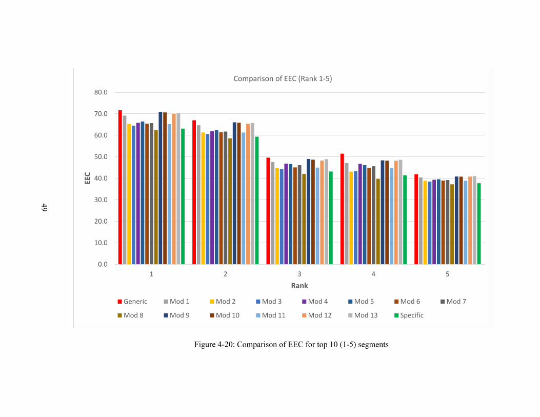
49
Figure 4-20: Comparison of EEC for top 10 (1-5) segments
0.0
10.0
20.0
30.0
40.0
50.0
60.0
70.0
80.0
1 2 3 4 5
EEC
Rank
Comparison of EEC (Rank 1-5)
Generic Mod 1 Mod 2 Mod 3 Mod 4 Mod 5 Mod 6 Mod 7
Mod 8 Mod 9 Mod 10 Mod 11 Mod 12 Mod 13 Specific
49
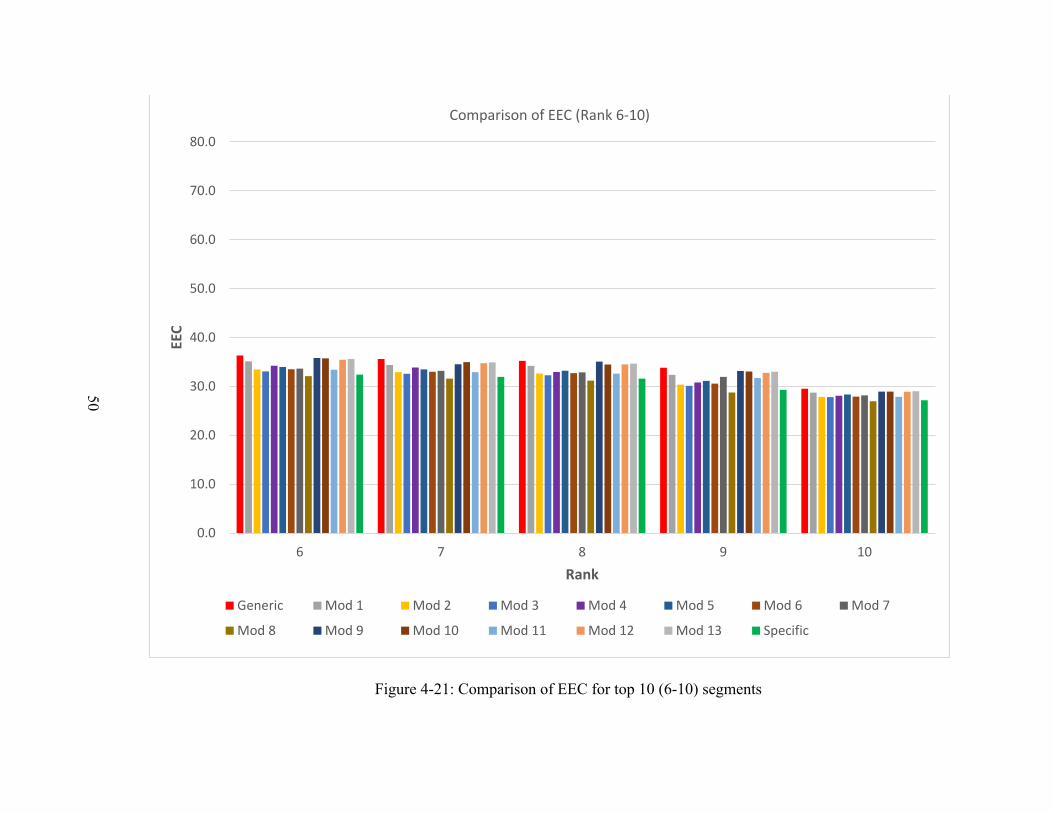
50
Figure 4-21: Comparison of EEC for top 10 (6-10) segments
0.0
10.0
20.0
30.0
40.0
50.0
60.0
70.0
80.0
6 7 8 9 10
EEC
Rank
Comparison of EEC (Rank 6-10)
Generic Mod 1 Mod 2 Mod 3 Mod 4 Mod 5 Mod 6 Mod 7
Mod 8 Mod 9 Mod 10 Mod 11 Mod 12 Mod 13 Specific
50

51
4.4.3 Comparison of Standard Error
Before drawing any conclusion from the magnitudes of EEC, the evaluation of standard
error might be useful. This is because EECs with vastly different standard deviation can
widen the ranges estimated by different models even more. The EEC of a segment is
represented by the following equation where the standard error (σ) is calculated using
equation 16.
𝐄𝐄𝐄𝐄𝐂𝐂 = (𝐸𝐸𝐸𝐸 𝐸𝐸𝐼𝐼𝑆𝑆𝐼𝐼𝑆𝑆𝑉𝑉𝑆𝑆𝑆𝑆𝑐𝑐 𝐶𝐶𝐼𝐼𝑉𝑉𝐼𝐼ℎ𝑆𝑆𝐼𝐼 − 𝑆𝑆𝑆𝑆𝐶𝐶 𝑆𝑆𝐼𝐼𝑆𝑆𝑐𝑐𝐼𝐼𝐼𝐼𝑆𝑆𝑆𝑆𝑐𝑐 𝐶𝐶𝐼𝐼𝑉𝑉𝐼𝐼ℎ𝑆𝑆𝐼𝐼) ± 𝜎𝜎
For the top 10 segments, the standard deviations are calculated. Here, the output of only
three models (i.e. “generic”, “specific” and model 8) are shown in Figure 4-22. Each bar
presents the EEC of any specific ranked segment with standard error bars. Though the
EECs are different for any particular rank, the figure below shows that the standard errors
of those segments are quite similar. For example, the standard error of the highest-ranked
site is around 7.5 and the 10th ranked segment is around 5 for all three SPFs.
Figure 4-22: Comparison of EEC with standard error
0.0
10.0
20.0
30.0
40.0
50.0
60.0
70.0
80.0
90.0
1 2 3 4 5 6 7 8 9 10
EEC
Rank
Comparison of EEC with standard error
Generic model EEC Model 8 EEC Speciifc Model

52
Chapter 5. CONCLUSION
This chapter will summarize the key findings of the study from the analysis. Following
that, it will discuss the limitations and provide recommendations to consider for future
study.
5.1 Summary
One of the advantages of using a “generic” SPF is that it does not require any adjustment
factors to adjust the predicted crashes since the entire dataset is involved to develop the
model. This is even more effective when the AFs are not available for a particular attribute
of any roadway type. But a “generic” SPF has several drawbacks too. For any roadway
type, a generic model will possibly have the worst CURE plot with poor goodness-of-fit
metrics indicating an undesirable model. On the other hand, a model developed from
specific value or ranges of base conditions with an overall better fit is very tempting to use.
But in the absence of appropriate AFs, this model will not be able to be adjusted for base
conditions. This study aimed to evaluate the trade-off between these two types of SPFs.
The major findings of this study are summarized below:
• Segment-level network screening:
Segment rank is nearly insensitive to the choice of the SPF. That means SPFs
developed from the entire dataset or any particular portion of the dataset (specified
by base conditions) produce quite similar ranked candidate lists. In such cases,
using a generic model developed from the entire dataset is usually more feasible to
use since it does not require any AFs. Developing AFs may not justify the cost of
segment-level network screening.
• Project-level analysis and others:
A generic SPF may not work as well for project-level analysis. Estimating the
benefit-cost ratio for a site, and other design-level decisions benefit from a more
accurate model.

53
Though all of the 15 SPFs developed in this thesis provided similar ranks,
the magnitude of the EECs for the segments varied model to model. For
example, using the generic model, the highest-ranked segment had an EEC
of 72 and a standard error of ±8. Using model 8 produced an EEC of 62
and a standard error of ±7.
In this study, the generic model overestimates the highest average EECs
amongst the models. Using FHWA and NHTSA numbers (6 million crashes
per year costing about $230 billion), the average cost per crash is around
$40,000. For the highest-ranked segment of rural two-lane roads in
Kentucky, the generic SPF overestimates EEC by 9 crashes compared to the
lowest model, a difference of around $360,000 in potential expected
benefits. Benefit-cost analysis is, therefore, more sensitive than network
screening/ranking to the choice of SPF.
The magnitude of the EEC is more important for project-level network
analysis. Project extents are usually described by a combination of several
segments, with project EEC being computed as the sum of the all project
segment EECs. The overestimation of the EEC values will affect the overall
project EEC.
Using ranges of values instead of a specific value for any attribute for SPF
development is suggested. Before applying the ranges, the “specific” model
seemed to the best performing model. But the ranges of attributes offered
improvements to the modeling process.
5.2 Limitations and Future Recommendations
The results from this study should be interpreted keeping the following the limitations in
mind:
• According to the HSM and several other studies (e.g. (Hauer and Bamfo, 1997;
Lord et al., 2005; Ogle et al., 2011), the minimum length of the homogenous
segments should be set to 0.1 mi. This is because shorter lengths can lead to a large
number of zero-crash segments which might affect the development of a valid SPF.

54
Any segment with a length shorter than 0.1 mi should either be removed from the
dataset or readjusted to adjacent segments. But, in this study, the minimum segment
length was taken as 0.05 mi (suggested by (Miaou, 1993)) because dropping the
segments with length less than 0.1 mi would have reduced the sample size
significantly and would have taken away almost half of the crashes. Therefore, for
future studies, segmentation and reassembly of the dataset based on the geometric
attributes might be redone considering the minimum segment length to be 0.1 mi.
• In this study, Negative Binomial (NB) method was used for regression because in
general, since crash data are counts and they do not follow a Poisson distribution.
NB regression accounts for the overdispersion of the data. The crash data used in
this thesis is significantly overdispersed with almost 70% segments with zero
crashes. In such cases, Zero Inflated Negative Binomial regression might be an
option for developing SPFs since this model can account for the predominance of
excessive zeros (Lord et al., 2005).
• The study was performed using the dataset for rural two-lane roadways in Kentucky
because important adjustment factors were available for this road type. Therefore,
it was possible to evaluate the effect of the availability and non-availability of AFs
on network screening. For additional assessments, urban highways or multilane
roads with more complex geometric characteristics can be studied using the same
methodology outlined in this work.
• In this study, SPFs were developed using all crashes (all severity levels combined
for a given location). A segment with 10 fatal and 10 injury crashes would be treated
the same as another with 2 fatal and 18 injury crashes. It is recommended that SPFs
for specific severities or perhaps even specific types of crashes be developed. In
this case, the modeler will be trading specificity and policy sensitivity against
sample size and accuracy.

55
REFERENCES
AASHTO, 2010. Highway Safety Manual, First Edition. American Association of State Highway and Transportation Officials, Washington, D.C.
Agent, K.R., O’Connell, L., Green, E.R., Kreis, D., Pigman, J.G., Tollner, N., Thompson, E.C., 2003. Development of procedures for identifying high-crash locations and prioritizing safety improvements.
Ahmed, M., Chalise, R., 2018. Calibration of the Highway Safety Manual’s Safety Performance Functions for Rural Two-Lane Highways with Regional Considerations for the Rocky Mountains and Plain Regions (No. MPC 18-344).
Bahar, G., Hauer, E., 2014. User’s Guide to Develop Highway Safety Manual Safety Performance Function Calibration Factors (No. HR 20-7(332)). NCHRP.
Blackden, C., Green, E., Souleyrette, R., Staats, W., 2018. Automating Safety Performance Function Development to Improve Regression Models.
Bornheimer, C., 2011. Finding a new safety performance function for two-way, two-lane highways in rural areas (PhD Thesis). University of Kansas.
Brimley, B.K., Saito, M., Schultz, G.G., 2012. Calibration of Highway Safety Manual Safety Performance Function: Development of New Models for Rural Two-Lane Two-Way Highways. Transp. Res. Rec. J. Transp. Res. Board 2279, 82–89. https://doi.org/10.3141/2279-10
FHWA Road Safety Audit Guidelines, 2006. . FHWA-SA-06-06 87. Gates, T., Savolainen, P., Avelar, R., Geedipally, S., Lord, D., Ingle, A., Stapleton, S.,
others, 2018. Safety Performance Functions for Rural Road Segments and Rural Intersections in Michigan (Technical Report No. SPR-1645). Michigan. Dept. of Transportation. Research Administration.
Green, E., 2018. Segmentation Strategies for Road Safety Analysis (Dissertation). University of Kentucky.
Hariharan, B., 2015. Functional Form and Heterogeneity on Safety Performance Function Estimation (Dissertation). The Pennsylvania State University.
Hauer, E., Bamfo, J., 1997. Two tools for finding what function links the dependent variable to the explanatory variables, in: Proceedings of the ICTCT 1997 Conference, Lund, Sweden.
Hauer, E., Harwood, D.W., Council, F.M., Griffith, M.S., 2002. Estimating safety by the empirical Bayes method: a tutorial. Transp. Res. Rec. 1784, 126–131.
Illinois Department of Transportation, 2014. AASHTO Highway Safety Manual Illinois User Guide with Illinois Calibration Factor and Default Values. Illinois Department of Transportation.
Jovanis, P.P., Chang, H.-L., 1986. Modeling the relationship of accidents to miles traveled. Transp. Res. Rec. 1068, 42–51.

56
Kuang, Y., Qu, X., Yan, Y., 2017. Will higher traffic flow lead to more traffic conflicts? A crash surrogate metric based analysis. PLoS One 12, e0182458.
Kuhn, M., Johnson, K., 2019. Feature engineering and selection: A practical approach for predictive models. CRC Press.
Lord, D., Washington, S.P., Ivan, J.N., 2005. Poisson, Poisson-gamma and zero-inflated regression models of motor vehicle crashes: balancing statistical fit and theory. Accid. Anal. Prev. 37, 35–46.
Lyon, C., Persaud, B., Gross, F., 2016. The Calibrator: An SPF Calibration and Assessment Tool User Guide 98.
Miaou, S.-P., 1993. The relationship between truck accidents and geometric design of road sections: Poisson versus negative binomial regressions. Oak Ridge National Lab., TN (United States).
Miaou, S.-P., Lum, H., 1993. Modeling vehicle accidents and highway geometric design relationships. Accid. Anal. Prev. 25, 689–709.
Nicholson, A., Wong, Y.-D., 1993. Are accidents poisson distributed? A statistical test. Accid. Anal. Prev. 25, 91–97.
Ogle, J.H., Alluri, P., Sarasua, W.A., 2011. Model minimum uniform crash criteria and minimum inventory roadway elements: Role of segmentation in safety analysis.
Persaud, B., Lyon, C., 2006. Safety performance assessment of freeway interchanges, ramps, and ramp terminals. Transp. Assoc. Can.
Resende, P.T.V., Benekohal, R.F., 1997. Effects of roadway section length on accident modeling, in: Traffic Congestion and Traffic Safety in the 21st Century: Challenges, Innovations, and OpportunitiesUrban Transportation Division, ASCE; Highway Division, ASCE; Federal Highway Administration, USDOT; and National Highway Traffic Safety Administration, USDOT.
Scopatz, R.A., Smith, S., 2016. Pennsylvania’s State-Specific SPFs and CMFs: Roadway Safety Data and Analysis Case Study (No. FHWA-SA-16-062). FHWA.
Souleyrette, R.R., Tanzen, R., Staats, W.N., Green, E.R., Chen, M., 2019. Safety Analysis for SHIFT Implementation.
Srinivasan, R., Bauer, K., 2013. Safety Performance Function Development Guide: Developing Juridiction-Specific SPFs (Final Report No. FHWA-SA-14-005). Federal Highway Administration Office of Safety.
Srinivasan, R., Carter, D., Bauer, K., 2013. Safety Performance Function Decision Guide: SPF Calibration versus SPF Development (No. FHWA-SA-14-004). FHWA.
Srinivasan, R., Gross, F., Lan, B., Bahar, G., 2016. Reliability of Safety Management Methods: Network Screening (Final Report No. FHWA-SA-16-037). Federal Highway Administration Office of Safety, Washington, DC.
Varoquaux, G., 2018. Cross-validation failure: small sample sizes lead to large error bars. Neuroimage 180, 68–77.

57
Wu, K.-F., Himes, S.C., Pietrucha, M.T., 2012. Evaluation of effectiveness of the federal highway safety improvement program. Transp. Res. Rec. 2318, 23–34.
Wu, L., Lord, D., Geedipally, S.R., 2017. Developing Crash Modification Factors for Horizontal Curves on Rural Two-Lane Undivided Highways Using a Cross-Sectional Study. Transp. Res. Rec. 2636, 53–61.
Wu, L., Lord, D., Zou, Y., 2015. Validation of Crash Modification Factors Derived from Cross-Sectional Studies with Regression Models. Transp. Res. Rec. J. Transp. Res. Board 2514, 88–96. https://doi.org/10.3141/2514-10
Yang, Y., 2007. Consistency of cross validation for comparing regression procedures. Ann. Stat. 35, 2450–2473. https://doi.org/10.1214/009053607000000514
Zhang, Y., Ye, Z., Lord, D., 2007. Estimating dispersion parameter of negative binomial distribution for analysis of crash data: bootstrapped maximum likelihood method. Transp. Res. Rec. 2019, 15–21.

58
VITA
RIANA TANZEN
Education
Masters of Science in Civil Engineering University of Kentucky
May 2018-Present
Bachelor of Science in Civil Engineering Bangladesh University of Engineering and Technology
April 2016
Professional Experience
Graduate Research Assistant Department of Civil Engineering, University of Kentucky
May 2018-Present
Lecturer Department of Civil Engineering, Presidency University, Bangladesh
Sep 2017 – Dec 2018
Awards
Winner of SDITE Traffic Bowl 2018 as a representative of the University of Kentucky
Publications
Souleyrette, R. R., Tanzen, R., Staats, W. N., Green, E. R., & Chen, M. (2019). Safety Analysis for SHIFT Implementation.
Tanzen, R., Souleyrette, R., Green, ER (2019). “Are the Benefits of Adjustment Factors for Safety Performance Functions Worth the Cost?”. Poster session presented at Road Safety and Simulation Conference 2019, Iowa, USA.
Tanzen, R.; Hoque, J.M., and Islam, S., (2018). “Predicting Highway Crash Frequency: A Review of Statistical Regression Models”. Journal of Modern Science and Technology Vol. 6, No. 1, pp.87-99.
Tanzen, R, Sultana, T., Islam, M.S. and Khan, A.J.; (2016) “Determination of Plastic Limit using Cone Penetrometer”. 3rd International Conference on Advances in Civil Engineering. CUET, Chittagong, Bangladesh.
Islam, M.S., Salma, U., Shuvo, M.R., and Tanzen, R.; (2016) “Study on river bank failure due to seepage”, 1st Bangladesh Civil Engineering Summit, BUET, Dhaka, Bangladesh.

59
Collegiate Activities
Member/ Vice President Institute of Transportation Engineers
May 2018-Present/Aug 2019- Present
Member/GradSWE Liaison Society of Women in Engineering
Jan 2019-Present/Sep 2019-Present
Member American Society of Civil Engineers Oct 2019-Present