NBER WORKING PAPER SERIES

THE RESPONSE OF CONSUMER SPENDING TO CHANGES IN GASOLINE PRICES

Michael GelmanYuriy Gorodnichenko

Shachar KarivDmitri Koustas

Matthew D. ShapiroDan SilvermanSteven Tadelis

Working Paper 22969http://www.nber.org/papers/w22969

NATIONAL BUREAU OF ECONOMIC RESEARCH1050 Massachusetts Avenue

Cambridge, MA 02138December 2016, Revised November 2017

This research is carried out in cooperation with a financial aggregation and bill-paying computer and smartphone application (the “app”). We are grateful to the executives and employees who have made this research possible. This research is supported by a grant from the Alfred P. Sloan Foundation. Shapiro acknowledges additional support from the Michigan node of the NSF-Census Research Network (NSF SES 1131500). Gorodnichenko thanks the NSF for financial support. We thank Arlene Wong and conference participants at NBER EFG and NBER SI (Consumption: Micro to Macro) for comments on an earlier draft of the paper. The views expressed herein are those of the authors and do not necessarily reflect the views of the National Bureau of Economic Research.

NBER working papers are circulated for discussion and comment purposes. They have not been peer-reviewed or been subject to the review by the NBER Board of Directors that accompanies official NBER publications.

© 2016 by Michael Gelman, Yuriy Gorodnichenko, Shachar Kariv, Dmitri Koustas, Matthew D. Shapiro, Dan Silverman, and Steven Tadelis. All rights reserved. Short sections of text, not to exceed two paragraphs, may be quoted without explicit permission provided that full credit, including © notice, is given to the source.

The Response of Consumer Spending to Changes in Gasoline PricesMichael Gelman, Yuriy Gorodnichenko, Shachar Kariv, Dmitri Koustas, Matthew D. Shapiro, Dan Silverman, and Steven TadelisNBER Working Paper No. 22969December 2016, Revised November 2017JEL No. E21,Q41,Q43

ABSTRACT

This paper estimates how overall consumer spending responds to changes in gasoline prices. It uses the differential impact across consumers of the sudden, large drop in gasoline prices in 2014 for identification. This estimation strategy is implemented using comprehensive, high-frequency transaction-level data for a large panel of individuals. The estimated marginal propensity to consume (MPC) out of unanticipated, permanent shocks to income is approximately one. This estimate takes into account the elasticity of demand for gasoline and potential slow adjustment to changes in prices. The high MPC implies that changes in gasoline prices have large aggregate effects.

Michael GelmanDepartment of Economics University of MichiganAnn Arbor MI 48109-1220 mgelman@umich.edu

Yuriy Gorodnichenko Department of Economics530 Evans Hall #3880 University of California, Berkeley Berkeley, CA 94720-3880and IZAand also NBERygorodni@econ.berkeley.edu

Shachar KarivDepartment of Economics University of California, Berkeley Berkeley, CA 94720kariv@berkeley.edu

Dmitri KoustasDepartment of Economics530 Evans Hall #3880 University of California, BerkeleyBerkeley, CA 94720-3880dkoustas@econ.berkeley.edu

Matthew D. ShapiroDepartment of EconomicsUniversity of Michigan611 Tappan StAnn Arbor, MI 48109-1220and NBERshapiro@umich.edu

Dan SilvermanDepartment of EconomicsW.P. Carey School of BusinessArizona State UniversityP.O. Box 879801Tempe, AZ 85287-9801and NBERDaniel.Silverman.1@asu.edu

Steven TadelisHaas School of BusinessUniversity of California, Berkeley545 Student Services BuildingBerkeley, CA 94720and NBERstadelis@haas.berkeley.edu

An online appendix is available at http://www.nber.org/data-appendix/w22969

I. Introduction

Few macroeconomic variables grab headlines as often and dramatically as do oil prices. In 2014,

policymakers, professional forecasters, consumers and businesses all wondered how the decline of

oil prices from over $100 per barrel in mid-2014 to less than $50 per barrel in January 2015 would

influence disposable incomes, employment, and inflation. A key component for understanding

macroeconomic implications of this shock is consumers’ spending from the considerable resources

freed up by lower gasoline prices (the average saving was more than $1,000, or approximately 2

percent of total spending per household).1 Estimating the quantitative impact of such changes is

central to policy decisions. Yet, because of data limitations, a definitive estimate has proved elusive.

Recently, “big data” has opened unprecedented opportunities to shed new light on the matter. This

paper uses detailed transaction-level data provided by a personal financial management service to

assess the spending response of consumers to changes in gasoline prices over the 2013-2016 period.

Specifically, we use this information to construct high-frequency measures of spending on

gasoline and on non-gasoline items for a panel of more than half a million U.S. consumers. We

use cross-consumer variation in the intensity of spending on gasoline interacted with the large,

exogenous, and permanent decline in gasoline prices to identify and estimate the partial

equilibrium marginal propensity to consume (MPC) out of savings generated by reduced gasoline

prices. Given the low elasticity of demand for gasoline and the nature of the oil price shock, one

can think of this MPC as measuring the response of spending to a permanent, unanticipated income

shock. Our baseline estimate of the MPC is approximately one. That is, consumers on average

spend all of their gasoline savings on non-gasoline items. There are lags in adjustment, so the

strength of the response builds over a period of weeks and months.

Our results are useful and informative in several dimensions. First, our estimate of the MPC

is largely consistent with the permanent income hypothesis (PIH), a theoretical framework that

became a workhorse for analyses of consumption, and that has been challenged in previous studies.

Second, our findings suggest that, ceteris paribus, falling oil prices can give a considerable boost

to the U.S. economy via increased consumer spending (although other factors can offset output

growth). Third, and also consistent with the PIH, we show that consumers’ liquidity was not

important for the strength of the consumer spending response to gasoline price shocks. Fourth, our

1 According to the U.S. Consumer Expenditure Survey, average total household spending in 2014 was $53,495 total, while the average household spending on gasoline was $2,468.

2

analysis highlights the importance of having high-frequency transaction data at the household level

for estimating consumer reactions to income and price shocks.

This paper is related to several strands of research. The first strand, surveyed in Jappelli

and Pistaferi (2010), is focused on estimating consumption responses to income changes.

Typically, studies in this area examine if and how consumers react to anticipated, transitory

income shocks and, like ours approach, provide the partial equilibrium response of household

spending to a shock, not the general equilibrium outcome for aggregates. A common finding in

this strand of research is that, in contrast to predictions of the PIH, consumers often spend only

upon the realization of an income shock, rather than upon its announcement, although the size of

this “excess sensitivity” depends on household characteristics. Baker (2016) and Kueng (2015)

document this pattern using data similar to what we study here and Gelman et al. (2016) report it

for the same data source that we use.

At the same time, estimating spending responses to unanticipated, highly persistent income

shocks has been challenging, because identifying such shocks is particularly difficult.2 Indeed, we

are not aware of an estimate of the MPC from this kind of shock. Thus, in sharp contrast to existing

literature, we possibly provide the first estimate of MPC for an unanticipated, permanent shock to

income. To this end, we exploit a particularly clear-cut source of variation in household budgets

(spending on gasoline) with a number of desirable properties. Specifically, we use a large, salient,

unanticipated, permanent (or perceived to be permanent) shock. We examine spending responses at

the weekly frequency while, due to data limitations, the vast majority of previous studies estimate

responses at much lower frequencies. As we discuss below, the high-frequency dimension allows us

to obtain crisp estimates of the MPC and thus provide a more informative input for policy making.

The second strand to which we contribute studies the effects of oil prices on the economy.

In surveys of this literature, Hamilton (2008) and Kilian (2008) emphasize that oil price shocks

can influence aggregate outcomes via multiple channels (e.g., consumer spending, changes in

2 Previous studies examined responses of consumption to highly persistent income shocks due to job displacements (e.g., Stephens 2001) or health (e.g., Gertler and Gruber 2002). However, these income shocks are likely combined with other changes in the lives of affected consumers which makes identification of MPC challenging. An alternative strategy is to use statistical decompositions in spirit of Japelli and Pistafferi (2006) but these estimates of MPC may depend on the assumptions of statistical models. Changes is taxes may provide a useful source of variation (see e.g. Neri et al. 2017) but it is often hard to identify the timing of these shocks (tax changes are typically announced well before the changes are implemented) and the persistence of shocks (tax changes could be reversed with a change in government).

3

expectations) but disruption of consumers’ (and firms’) spending on goods other than energy is

likely to be a key mechanism for amplification and propagation of the shocks. Indeed, given the

low elasticity of demand for gasoline, changes in gasoline prices can materially affect non-gasoline

spending budgets for a broad array of consumers. As a result, a decrease in gasoline prices can

generate considerable savings for consumers which could be put aside (e.g., to pay down debt or

save) or used to spend on items such as food, clothing, furniture, etc.

Despite the importance of the MPC out of gasoline savings, research on the sensitivity of

consumer non-gasoline spending to changes in the gasoline price, has been scarce. One reason for the

scarcity of research on the matter has been data limitations. Available household consumption data

tend to be low frequency, whereas consumer spending, gasoline prices, and consumer expectations

can change rapidly. For example, the interview segment of the U.S. Consumer Expenditure Survey

(CEX) asks households to recall their spending over the previous month. These data likely suffer from

recall bias and other measurement errors that could attenuate estimates of households’ sensitivity to

changes in gasoline prices (see Committee on National Statistics 2013). The diary segment of the

CEX has less recall error, but the panel dimension of the segment is short (14 days), making it difficult

to estimate the consumer response to a change in prices. Because the CEX is widely used to study

consumption, we do a detailed comparison of our approach using the app data with what can be

learned from using the CEX. We find that analysis of the CEX produces much noisier estimates.

Grocery store barcode data, such as from AC Nielsen, have become a popular source to

measure higher-frequency spending. These data, however, cover only a limited category of goods.

For example, gasoline spending by households is not collected in AC Nielsen, making it impossible

to exploit heterogeneity in gasoline consumption across households. As a result, most estimates of

MPC tend to be based on time series variation in aggregate series (see e.g. Edelstein and Kilian 2009).

There are a few notable exceptions. Using loyalty cards, Hastings and Shapiro (2013) are

able to match grocery barcode data to gasoline sold at a large grocery store retailer with gasoline

stations on site. We show that households typically visit multiple gasoline station retailers in a

month, suggesting limitations to focusing on consumer purchases at just one retailer. There is also

some recent work using household data to identify a direct channel between gasoline prices and

non-gasoline spending. Gicheva, Hastings and Villas-Boas (2010) use weekly grocery store data

to examine the substitution to sale items as well as the response of total spending. They find that

4

households are more likely to substitute towards sale items when gasoline prices are higher, but

they must focus only on a subset of goods bought in grocery stores (cereal, yogurt, chicken and

orange juice), making it difficult to extrapolate.

Perhaps the closest work to ours is a policy report produced by the J.P. Morgan Chase

Institute (2015), which also uses “big data” to examine the response of consumers to the 2014 fall

in gasoline prices, and finds an average MPC of approximately 0.6. This report differs from our

study in both its research design and its data. Most importantly, our data include a comprehensive

view of spending, across many credit cards and banks. In contrast, the Chase report covers a vast

number of consumers, but information on their spending is from Chase accounts only. If, for

example, consumers use a non-Chase credit card or checking account, any spending on that

account would be missed in the J.P. Morgan Chase Institute analysis, and measurement of

household responses may therefore be incomplete. In this paper, we confirm this by showing that

an analysis based on accounts in one financial institution leads to a significantly attenuated

estimate of the response of spending to changes in gasoline prices.

This paper proceeds as follows. Section II describes trends in gasoline prices, putting the

recent experience into historical context. In Section III, we discuss the data, Section IV describes our

empirical strategy, and Section V presents our results. Specifically, we report baseline estimates of

the MPC and the elasticity of demand for gasoline. We contrast these estimates with the comparable

estimates one can obtain from alternative data. In Section V we also explore robustness of the

baseline estimates and potential heterogeneity of responses across consumers. Section VI concludes.

II. Recent Changes in Gasoline Prices: Unanticipated, Permanent and Exogenous

In this section, we briefly review recent dynamics in the prices of oil and gasoline and corresponding

expectations of future prices. We document that the collapse of oil and gasoline prices in 2014-2015

was highly persistent, unanticipated, and exogenous to demand conditions in the United States.

These properties of the shock are important components of our identification strategy.

A. Unanticipated and Permanent

In Panel A of Figure 1, the solid black line shows the spot price of gasoline at New York Harbor,

an important import and export destination for gasoline. The New York Harbor price is on average

5

70 cents lower than average retail prices, although the two series track each other very closely.

The dashed line shows the one-year-ahead futures price for that date. The futures price tracks the

spot price closely, suggesting the market largely treats gasoline price as a random walk—i.e., the

best prediction for one-year-ahead price is simply the current price.

Panel B shows the difference between the realized and predicted spot price. The behavior

of one-year-ahead forecast errors indicates that financial markets anticipated neither the run-up

nor the collapse of gasoline prices in 2007-2009. Likewise, the dramatic decline in gasoline prices

in 2014-2015 was not anticipated.

The Michigan Survey of Consumers has asked households about their expectations for

changes in gasoline prices over the next one-year and five-year horizons. Panel C of Figure 1 plots

the mean and median consumer expectations along with the actual price and the mean one-year-

ahead prediction in the Survey of Professional Forecasters. While consumers expect a slightly

higher price relative to the present price than professional forecasters, the basic pattern is the same

as in Panel A: the current price appears to be a good summary of expected future prices. Consistent

with this observation, Anderson, Kellogg and Sallee (2012) fail to reject the null of a random walk

in consumer expectations for gasoline prices. Thus, consumers perceive changes in gasoline prices

as permanent. Also similar to the financial markets, consumers were not anticipating large price

changes in 2007-2009 or 2014-2015 (Panel D).

Figure 1 shows large movements in prices during the Great Recession (shaded). Unlike the

recent episode that is the subject of this paper, we would not use it to identify the MPC because

this fluctuation in commodity prices in the Great Recession surely represents an endogenous

response to aggregate economic conditions.

When put into historical context, the recent volatility in gasoline prices is large. Table 1

ranks the largest one-month percent changes in oil prices since 1947. When available, the change

in gasoline prices over the same period is also shown.3 The price drops in 2014-2015 are some of

the largest changes in oil and gasoline prices in the last 60 years. Note that in 1986, gasoline prices

3 Oil spot prices exist back to 1947, while the BLS maintains a gasoline price series for urban areas back to 1976. In our analysis, we use AAA daily gasoline prices retrieved from Bloomberg (3AGSREG). The series comes from a daily survey of 120,000 gasoline stations. These data almost perfectly track another series from the EIA which are point in-time estimates from a survey of 900 retail outlets as of 8am Monday.

6

and oil prices actually moved in opposite directions, indicating that the process generating gasoline

prices can sometimes differ from oil.

B. Exogenous

Why did prices of oil and oil products such as gasoline fall so much in 2014-2015? While many

factors could have contributed to the dramatic decline in the prices, the consensus view, summarized

in Baffes et al. (2015), attributes a bulk of the decline to supply-side factors. Specifically, this view

emphasizes that key forces behind the decline were, first, OPEC’s decision to abandon price support

and, second, rapid expansion of oil supply from alternative sources (shale oil in the U.S., Canadian

oil sands, etc.). Consistent with this view, other commodity prices had modest declines during this

period, which would not have happened if the decline in oil prices was driven by global demand

factors. Observers note that the collapse of oil prices in 2014-2015 is similar in many ways to the

collapse in 1985-1986, when more non-OPEC oil supply came from Mexico, the North Sea and

other sources, and OPEC also decided to abandon price support. In short, available evidence suggests

that the 2014-2015 decline in oil prices is a shock that was supply-driven and exogenous to U.S.

demand conditions. In contrast, Hamilton (2009) and others observe that the run up in oil and

gasoline prices around 2007-2009 can be largely attributed to booming demand, stagnant production,

and speculators, and the consequent decline of the prices during this period, to collapsed global

demand (e.g. the Great Recession and Global Financial Crisis).

III. Data

Our analysis uses high-frequency data on spending from a financial aggregation and bill-paying

computer and smartphone application (henceforth, the “app”).4 The app had approximately 1.4

million active users in the U.S. in 2013.5 Users can link almost any financial account to the app,

including bank accounts, credit card accounts, utility bills, and more. Each day, the app logs into

the web portals for these accounts and obtains central elements of the user's financial data including

4 These data have previously been used to study the high-frequency responses of households to shocks such as the government shutdown (Gelman et al. 2016) and anticipated income, stratified by spending, income and liquidity (Gelman et al. 2014). 5All data are de-identified prior to being made available to the project researchers. Analysis is carried out on data aggregated and normalized at the individual level. Only aggregated results are reported.

7

balances, transaction records and descriptions, the price of credit and the fraction of available credit

used. Using data for a similar service, Baker (2016) documents that over 90 percent of users link

all their checking, savings, credit card, and mortgage accounts. Given the non-intrusive automatic

data collection, attrition rates are moderate (approximately five percent per quarter).

We draw on the entire de-identified population of active users and data derived from their

records from January 2013 until February 2016. The app does not collect demographic information

directly and, thus, we ar unable to study heterogeneity in responses across demographic groups or to

use weights or similar methods to correct possible imbalances in the population of the app’s users.

However, for a subsample of users, the app employed a third-party that gathers both public and

private sources of demographics, anonymizes them, and matches them back to the de-identified

dataset. Table 1 in Gelman et al. (2014) (replicated in Appendix Table C2) compares the gender,

age, education, and geographic distributions in a subset of the sample to the distributions in the U.S.

Census American Community Survey (ACS), representative of the U.S. population in 2012. The

app’s user population is heterogeneous (including large numbers of users of different ages, education

levels, and geographic location) and, along some demographic dimensions, contains proportions

similar to those found in the US population. Consistent with this pattern, Baker (2016) observes that,

as the online industry had matured, the differences between the population of a similar app’s users

and the U.S. population became small by 2013.

A. Identifying Spending Transactions

Not every transaction reported by the app is spending. For example, a transfer of funds from one

account to another is not. To avoid double counting, we exclude transfers across accounts, as well

as credit card payments from checking accounts that are linked within the app. If an account is not

linked, but we still observe a payment, we count this as spending when the payment is made. We

identify transfers in several ways. First, we search if a payment from one account is matched to a

receipt in another account within several days. Second, we examine transaction description strings

to identify common flags like “transfer”, “tfr”, etc. To reduce the chance of double counting, we

exclude the largest single transaction that exceeds $1,000 in a given week, as this kind of transaction

is very heavily populated by transfers, credit card payments, and other non-spending payments (e.g.,

payments to the U.S. Internal Revenue Service). We include cash withdrawals from the counter and

8

ATM in our measure of spending. To ensure that accounts in the app data are reasonably linked and

active, we keep all users who were in the data for at least 8 weeks in 2013 and who did not have

breaks in their transactions for more than two weeks. More details are provided in Appendix A.

B. Using Machine Learning to Classify Type of Spending

Our analysis requires classification of spending by type of goods. To do so, we address several

challenges in using transactional data from bank accounts and credit cards. First, transactional data

are at the level of a purchase at an outlet. For many purchases, a transaction will include many

different goods. In the case of gasoline, purchases are carried out mainly at outlets that exclusively

or mainly sell gasoline. Hence, gasoline purchases are relatively easy to identify in transactional

data. Second, for the bulk of transactions in our data, we must classify the outlet from the text of

the transaction description, rather than classifications provided by financial institutions. We

therefore use a machine learning (ML) algorithm to classify spending based on transaction

descriptions. In this section, we provide an outline of the classification routine, and compare our

ML predictions in the data provided by the app with external data. As economic analysis

increasingly uses naturally-occurring transactional data to replace designed survey data,

applications of ML like the one we use will be increasingly important.

The ML algorithm constructs a set of rules for classifying the data as gasoline or non-

gasoline. This requires a training data set to build a classification model, and a testing data set not

used in the training step to validate the model predictions. Two of the account providers in the data

classify spending directly in the transaction description strings, using merchant category codes

(MCCs). MCCs are four digit codes used by credit card companies to classify spending and are

also recognized by the U.S. Internal Revenue Service for tax reporting purposes. Our main MCC

of interest is 5541, “Automated Fuel Dispensers.” Purchases of gasoline could also fall into MCC

code 5542, “Service Stations,” which in practice covers gasoline stations with convenience stores.6

We group transactions with these two codes together because distinguishing transactions as 5542

or 5541 without the MCC is nearly impossible with only the transaction descriptions.7

6 “Service Stations” do not include services such as auto repairs, motor oil change, etc. 7 E.g., a transaction string with word “Chevron” or “Exxon” could be classified as either MCC 5541 or MCC 5542.

9

A downside of this approach is that transactions at a Service Station may either be for gasoline,

for food or other items, or both. According to the National Association of Convenience Stores

(NACS), which covers gasoline stations, purchases of non-gasoline items at gasoline stations with

convenience stores (i.e. “Service Stations”) account for about 30 percent of sales at “Service Stations.”

Although the app data do not permit us to differentiate gasoline and non-gasoline items at “Service

Stations,” we can use transaction data from “Automated Fuel Dispensers” (which do not have an

associated convenience store), as well as external survey evidence to separate purchases of non-

gasoline items from purchases of gasoline. Specifically, according to the 2015 NACS Retail Fuels

Report (NACS 2015), 35 percent of gasoline purchases are associated with going inside a gasoline

station’s store. Conditional on going inside the store, the most popular activities are to “pay for

gasoline at the register” (42%), “buy a drink” (36%), “buy a snack” (33%), “buy cigarettes” (24%),

and “buy lottery tickets” (22%). The last four items are likely to be associated with relatively small

amounts of spending. This conjecture is consistent with the distribution of transactions for “Service

Stations” and “Automated Fuel Dispensers” in the data we study. In particular, approximately 60

percent of transactions at “Service Stations” are less than $10 while the corresponding share for

“Automated Fuel Dispensers” is less than 10 percent. As we discuss below, the infrequent incidence

of gasoline purchases totaling less than $10 is also consistent with other data sources. Thus, we

exclude Service Stations transactions less than $10 to filter out purchases of non-gasoline items.

Using one of the two providers with MCC information (the one with more data), we train

a Random Forest ML model to create binary classifications of transactions into those made at a

gasoline station/service station and those that were made elsewhere. Figure 2 shows an example

of decision trees used to classify transactions into gasoline and non-gasoline spending. A tree is a

series of rules that train the model to classify a purchase as gasoline or not. The rules minimize

the decrease in accuracy when a particular model “feature,” in our case transaction values and

words in the transaction strings, is removed. In the Figure 2 example, the most important single

word is “oil.” If a transaction string contains the word oil, the classification rule is to move to the

right, otherwise the rule is to move to the left. If the string does not contain the word oil, the next

most important single word is “exxonmobil.” Figure 2 also demonstrates how the decision tree

combines transaction string keywords with transaction amounts. For example, “oil” is a very strong

10

predictor of gasoline purchase but it can be further refined by the transaction amount. The tree

continues until all the data are classified.

We then use the second provider to validate the quality of our ML model.8 The ML model

is able to classify spending with approximately 90% accuracy in the testing data set, which is a

high level of precision. Both Type I and Type II error rates are low. See Appendix Table B.1.

More details on the procedure can be found in Appendix B.

We can also use the app data to investigate which gasoline stations consumers typically

visit. The top ten chains of gasoline stations in the app data account for most of gasoline spending.

On average, the app data suggest that the typical consumer does 66 percent of his or her gasoline

spending in one chain and the rest of gasoline spending is spread over other chains. Thus, while

for a given consumer there is a certain degree of concentration of gasoline purchases within a

chain, an analysis focusing on only one gasoline retailer, such as in Gicheva, Hastings and Villas-

Boas (2010) or Hastings and Shapiro (2013), particularly one not in the top ten chains, would miss

a substantial amount of gasoline spending.

C. Comparison with the Consumer Expenditure Survey

We compare our measures of gasoline and non-gasoline spending with similar measures from the

Consumer Expenditure Survey (CEX).9 We use both the CEX Diary Survey and Interview Survey.

In the diary survey, households record all spending in written diaries for 14 days. Therefore, this

survey provides an estimate of daily gasoline spending that should be comparable to the daily

totals we observe in the app. In Figure 3, we compare the distribution of spending in our data (solid

lines) and in the diary survey (dashed line). We find that the distributions are very similar, with

one notable exception: the distribution of gasoline purchases in the app data has more mass below

$10 (solid gray line) than the CEX Diary data. As we discussed above, this difference is likely to

8 Card providers use slightly different transaction strings, and one may be concerned that training the model on a random subsample of data from both card providers, and testing it on another random subsample, can provide a distorted sense of how our ML model performs on data from other card providers. Thus, using a card from one account provider to train, and testing on an entirely different account provider, helps to assure that the ML model is valid outside of the estimation sample. Classification of transactions based on ML applied to both card providers yields very similar results. 9 While the definition of the spending unit is different in the CEX (“household”) and the app (“user”), Baker (2016) shows for a similar dataset that linked accounts generally cover the whole household.

11

be due to our inability to differentiate gasoline purchases and non-gasoline purchases at “Service

Stations.” In what follows, we restrict our ML predictions to be greater than $10 (solid black line).

The CEX Diary Survey provides a limited snapshot of households’ gasoline and other

spending. In particular, since a household on average only makes 1 gasoline purchase per week in

the diary, we expect only to observe 2 gasoline purchases per household, which can be a noisy

estimate of gasoline spending at the household level. Idiosyncratic factors in gasoline consumption

that might push or pull a purchase from one week to the next could influence the measure of a

household’s gasoline purchases by 50% or more. In addition, because the survey period in the

diary is so short, household fixed effects cannot be used to control for time-invariant household

heterogeneity. Hence, while a diary survey could be a substitute for the app data in principle, the

short sample of the CEX diary makes it a poor substitute in practice.10

The CEX Interview Survey provides a more complete measure of total spending, as well

as a longer panel (4 quarters), from which we can make a comparison with estimates based on

spending reported by the app at longer horizons. Panel A of Figure 4 reports the histogram (bin

size is set to $1 intervals) of monthly spending on gasoline in the CEX Interview data for 2013-

2014.11 The distribution has clear spikes at multiples of $50 and $100 with the largest spikes at $0

and $200. In contrast, the distribution of gasoline purchases in the app data has a spike at $0 but

the rest of the distribution exhibits considerably less bunching, particularly at large values like

$200 or $400 that correspond with reporting $50 or $100 per week, respectively. In addition, the

distribution of gasoline spending has a larger mass at smaller amounts in the app data than in the

CEX Interview data. These differences are consistent with recall bias in the CEX Interview Survey

data. As argued by Binder (2015), rounding in household surveys can reflect a natural uncertainty

of households about how much they spent in this category.

Table 2 compares moments for gasoline and non-gasoline spending across the CEX and

the app data. We find that the means are similar across data sources. For example, mean (median)

biweekly gasoline spending in the CEX Diary Survey is $84.72 ($65.00), while the app counterpart

10 We have done a comparison of the CEX diary spending for January 2013 through December 2014. In a regression of log daily spending for days with positive spending on month time effects and day of week dummies, the month effects estimated in the CEX and app have a correlation of 0.77. (Finer than monthly comparison of the app and CEX is not possible because the CEX provides only the month and day of week, but not the date, of the diary entry.) 11 The CEX Interview Survey question asks households to report their “Average monthly expense for gasoline.”

12

is $87.83 ($58.03). Similarly, mean (median) non-gasoline spending is $1,283 ($790.56) in the

CEX Diary Survey and $1,561.38 ($1,084.38) in the app data. The standard deviation (interquartile

range) tends to be a bit larger in the app data than in the CEX, which reflects a thicker right tail of

spending in the app data. This pattern is consistent with top-coding and under-representation of

higher-income households in the CEX, a well-documented phenomenon (Sabelhaus et al. 2015).

The moments in the CEX Interview Survey (quarterly frequency) are even closer to the moments

in the app data. For example, mean (median) spending on gasoline is $647 ($540) in the CEX

Interview Survey data and $628 ($475) in the app data, while the standard deviations (interquartile

ranges) are $531 ($630) and $588 ($660) respectively. In each panel of Table 2, we also compare

the distribution of the ratio of gasoline spending to non-gasoline spending, a central ingredient in

our analysis. The moments for the ratio in the CEX and the app data are similar. For instance, the

mean ratio is 0.08 for the CEX Interview Survey and 0.07 for the app data, while the standard

deviation of the ratio is 0.07 for both the CEX Interview Survey and the app data.12

In summary, spending in the app data is similar to spending in the CEX data. Thus, although

participation in the app is voluntary, app users have spending patterns similar to the population. In

addition to reflecting survey recall bias and top-coding, some of the differences could reflect

consumers buying gasoline on cards that are not linked to the app (such as credit cards specific to

gasoline station chains), the ML procedure missing some gasoline stations, or gasoline spending done

in cash that we could not identify. We will address these potential issues in our robustness tests.

IV. Empirical Strategy

The discourse on potential macroeconomic effects of a fall in gasoline prices centers on the

question of how savings from the fall in gasoline prices are used by consumers. Specifically,

policymakers and academics are interested in the marginal propensity to consume (MPC) from

savings generated by reduced gasoline prices.13 Define MPC as

12 Appendix Figure C1 shows the density of the gasoline to non-gasoline spending ratio for the CEX and app data. 13 For example, Janet Yellen (Dec 2014) compared the fall in gasoline prices to a tax cut: “[The decline in oil prices] is something that is certainly good for families, for households, it’s putting more money in their pockets, having to spend less on gas and energy, so in that sense it’s like a tax cut that boosts their spending power.”

13

∗ (1)

where i and t index consumers and time, is spending of non-gasoline items, is the price of

gasoline, and is the quantity of consumed gasoline. Note that we define the MPC as an increase

in spending (measured in dollars) in response to a dollar decrease in spending on gasoline after

the price of gasoline declines.14

Equation (1) is a definition, not a behavioral relationship. Of course, , the quantity of

gasoline purchased, and overall non-gasoline spending, , are simultaneously determined, with

simultaneity being an issue at the individual as well as aggregate level. In this section, we develop

an econometric relationship that yields identification of the MPC based on the specific sources of

variation of gasoline prices discussed in the previous sections.

At the aggregate level, one important determinant of gasoline spending is aggregate

economic conditions. As discussed in Section II, the 2007-2008 collapse in gasoline prices has

been linked to the collapse in global demand due to the financial crisis—demand for gasoline fell

driving down the price at the same time that demand was falling for other goods. Individual-level

shocks are another important source of simultaneity bias and threat to identification. Consider a

family going on a road trip to Disneyland; this family will have higher gasoline spending (long

road trip) and higher total consumption in that week due to spending at the park. Yet another

example is a person who suffers an unemployment spell; this worker will have lower gasoline

spending (not driving to work) and lower other spending (a large negative income shock).

This discussion highlights that gasoline purchases and non-gasoline spending are affected by

a variety of shocks. Explicitly modelling all possible shocks, some of which are expected in advance

by households (unobservable to the econometrician), would be impossible. Fortunately, this is not

required to properly identify the policy-relevant parameter–the sensitivity of non-gasoline spending

to changes in gasoline spending induced by exogenous changes in the price of gasoline. This

parameter may be interpreted as a partial derivative of non-gasoline spending with respect to the

price of gasoline and thus could be mapped to a coefficient estimated in a regression. For this, we

only need to satisfy a weaker set of conditions. First, we need exogenous, unanticipated shocks to

14 The MPC is likely different across groups of people, but our notation and estimation refers to the average MPC.

14

gasoline prices. These shocks should be unrelated to the regression residual absorbing determinants

of non-gasoline consumption unrelated to changes in gasoline prices. Second, we need to link non-

gasoline spending to the price of gasoline (i.e., , rather than purchases of gasoline ( ).

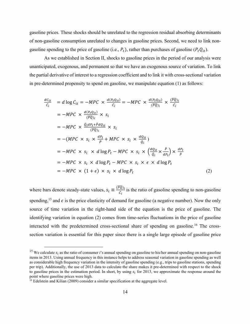
As we established in Section II, shocks to gasoline prices in the period of our analysis were

unanticipated, exogenous, and permanent so that we have an exogenous source of variation. To link

the partial derivative of interest to a regression coefficient and to link it with cross-sectional variation

in pre-determined propensity to spend on gasoline, we manipulate equation (1) as follows:

log

)

log

log log

1 log (2)

where bars denote steady-state values, ≡ is the ratio of gasoline spending to non-gasoline

spending,15 and is the price elasticity of demand for gasoline (a negative number). Now the only

source of time variation in the right-hand side of the equation is the price of gasoline. The

identifying variation in equation (2) comes from time-series fluctuations in the price of gasoline

interacted with the predetermined cross-sectional share of spending on gasoline.16 The cross-

section variation is essential for this paper since there is a single large episode of gasoline price

15 We calculate as the ratio of consumer i’s annual spending on gasoline to his/her annual spending on non-gasoline items in 2013. Using annual frequency in this instance helps to address seasonal variation in gasoline spending as well as considerable high frequency variation in the intensity of gasoline spending (e.g., trips to gasoline stations, spending per trip). Additionally, the use of 2013 data to calculate the share makes it pre-determined with respect to the shock to gasoline prices in the estimation period. In short, by using for 2013, we approximate the response around the point where gasoline prices were high. 16 Edelstein and Kilian (2009) consider a similar specification at the aggregate level.

15

movements in the sample period. One can also derive the specification from a utility maximization

problem and link the MPC to structural parameters (see Appendix D). Thus, regressing log non-

gasoline spending on the log of gasoline price multiplied by the ratio of gasoline spending to non-

gasoline spending yields an estimate of 1 .

Note that we have an estimate of −MPC scaled by 1 , but the scaling should be small if

demand is inelastic. As discussed below, there is some variation in the literature on ’s estimated using

household versus aggregate data. To ensure that a measure of is appropriate for our sample, we note:

log log log

log log 1 log 1 log . (3)

Similar to equation (2), the only source of time variation in the right-hand side of equation (3) is the

price of gasoline. Thus, a regression of log on log yields an estimate of elasticity 1 ,

which is the partial derivative of gasoline spending with respect to the price of gasoline, and the

residual in this regression absorbs determinants of gasoline purchases unrelated to the changes in the

price of gasoline.17 The estimated 1 and 1 can be combined to obtain the .

In the derivation of equations (2) and (3) we deliberately did not specify the time horizon

over which sensitivities are computed, as these may vary with the horizon. For example, with lower

prices, individuals may use their existing cars more intensively or may purchase less fuel-efficient

cars. There may be delays in adjustment to changes in prices (e.g., search for a product). It might

take time to notice the price change (Coibion and Gorodnichenko 2015). The very-short-run effects

may also depend on whether a driver’s tank is full or empty when the shock hits.

To obtain behavioral responses over different horizons, we build on the basic derivation

above and estimate a multi-period “long-differences” model, where both the MPC and the price

elasticity are allowed to vary with the horizon. Additionally, we introduce aggregate and

idiosyncratic shocks to overall spending, and idiosyncratic shocks to gasoline spending. Hence,

17 Because the dependent variable is spending on gasoline rather than volume of gasoline, elasticity ϵ estimated by this approach also includes substitution across types of gasoline (Hastings and Shapiro 2013).

16

Δ log Δ log (4)

Δ log Δ log (5)

where 1 , 1 , Δ is a k-period-difference operator,

is the time fixed effect, and and are individual-level shocks to spending.18 By varying , we

can recover the average impulse response over -periods so that we can remain agnostic about

how quickly consumers respond to a change in gasoline prices.19 Given that our specification is in

differences, we control for consumer time-invariant characteristics (gender, education, location,

etc.) as well as for the level effect of on non-gasoline spending. To minimize adverse effects of

extreme observations, we winsorize dependent variables Δ log and Δ log as well as

at the bottom and top one percent.

Because we are interested in the first-order effects of the fall in gasoline prices on consumer

spending, we include the time fixed effects in specification (4). As a result, we obtain our estimate

after controlling for common macroeconomic shocks and general equilibrium effects (e.g.,

changes in wages, labor supply, investment). Thus, consistent with the literature estimating MPC

for income shocks (e.g., Shapiro and Slemrod 2003, Johnson et al. 2006, Parker et al. 2008, Jappelli

and Pistaferi 2010), we estimate a partial equilibrium MPC.

We assume a common price of gasoline across consumers in this derivation. In fact the

comovement of gasoline prices is very strong (see Appendix Figure C2) and thus little is lost by

using aggregate gasoline prices. Furthermore, when computing we use gasoline spending rather

than gasoline prices and thus our measure of takes into account geographical differences in

levels of gasoline prices. We find nearly identical results when we use local gasoline prices.

Note that gasoline and oil prices are approximately random walks and thus Δ log can be

treated as an unanticipated, permanent shock. To the extent oil prices and, hence, gasoline prices are

18 Note that there are time effects only in equation (4). Since we have argued that changes in gasoline prices are exogenous over the time period, time effects are not needed for consistency of estimation of either (4) or (5). In (4), they may improve efficiency by absorbing aggregate shocks to overall spending. We cannot include time effects in (5) because they would completely absorb the variation in gasoline prices. But again note that the presence of an aggregate component in u does not make the estimates of δ biased under our maintained assumption that gasoline prices are exogenous to the U.S. economy in the estimation period. (The standard errors account for residual aggregate shocks.) 19 For example, if log ∑ and summarizes variation orthogonal to the shock series of interest, then the impulse response is and the long-difference regression recovers ∑ .

17

largely determined by global factors or domestic supply shocks, rather than domestic demand—

which is our maintained assumption for our sample period—OLS yields consistent estimates of

and . Formally, we assume that the idiosyncratic shocks to spending are orthogonal to these

movements in gasoline prices. Given the properties of the shock to gasoline prices in 2014-2015, the

PIH model predicts that the response of spending from the resulting change in resources should be

approximately equal to the change in resources ( 1) and take place quickly.

The approach taken in specifications (4) and (5) has several additional advantages

econometrically. First, as discussed in Griliches and Hausman (1986), using “long differences” helps

to enhance signal-to-noise ratio in panel data settings. Second, specifications (4) and (5) allow

straightforward statistical inference. Because our shock ( log ) is effectively national and we

expect serial within-user correlation in spending, we cluster standard errors on two dimensions: time

and person. This approach to constructing standard errors is much more conservative than the

common practice of clustering standard errors only by a consumer, employer, or location (e.g.,

Johnson et al. 2006, Levin et al. 2017). To make our results comparable to previous studies, we also

report standard errors clustered on user only. Third, although the variables are expressed in logs,

equation (2) shows that we estimate an rather than an elasticity and thus there is no need for

additional manipulation of the estimate. This aspect is important in practice because the distribution

of spending is highly skewed (in our data, the coefficient of skewness for weekly spending is

approximately four) and specifications estimating on levels of spending (rather than logs) are

likely sensitive to what happens in the right tail of the spending distribution. Finally, because oil and

gasoline prices change every day and the decline in the price of oil (and gasoline) was spread over

time, there is no regular placebo test on a “no change” period or before-after comparison. However,

these limitations are naturally addressed using regression analysis.

To summarize, our econometric framework identifies the from changes in gasoline

prices by interacting two sources of variation: a large, exogenous, and permanent change in

gasoline prices, with the pre-determined share of spending on gasoline. The econometric

specification also accounts for the response of spending on gasoline to lower prices by allowing a

non-zero elasticity of demand for gasoline and allowing for lagged adjustment of gasoline

spending to changes in gasoline prices.

18

V. Results

In this section, we report estimates of and for different horizons, frequencies, and

populations. We also compare estimates based on our app data to the estimates based on spending

data from the CEX.

A. Sensitivity of Expenditure to Gasoline Prices

We start our analysis with the estimates of and at weekly frequency for different response

horizons. Panel A of Figure 5 shows , and 95 percent confidence bands, for 0,… , 26 weeks.

Table 3, Row 1, gives the point estimates for selected horizons. The point estimates indicate that

the elasticity of demand for gasoline is increasing in the horizon (i.e., over time, consumers have

greater elasticity of demand): estimated elasticity changes from -0.20 at the horizon of 15 weeks

to -0.24 at the horizon of 25 weeks. When we use our preferred standard errors clustered by time

and user, confidence intervals are very wide at short horizons; estimates become quite precise at

horizons of 12 weeks and longer. In contrast, the conventional practice of clustering standard errors

by user yields tight confidence bands but these likely understate sampling uncertainty in our

estimates because there is considerable cross-panel dependence in the data.

This estimate is broadly in line with previously reported estimates. Using aggregate data, the

results in Hughes, Knittel and Sperling (2008) suggest that U.S. gasoline demand is significantly

more inelastic today compared with the 1970s. Regressing monthly data on aggregate per capita

consumption of gasoline on changes in gasoline prices, they estimate a short-run (monthly) price

elasticity of -0.034 to -0.077 for the 2001 to 2006 period, compared with -0.21 to -0.34 for the 1975-

1980 period. The Environmental Energy Institute (EIA 2014) also points to an elasticity close to

zero, and also argues this elasticity has been trending downward over time.20 In contrast to Hughes,

Knittel and Sperling (2008), our findings suggest that gasoline spending could still be quite

responsive to gasoline price changes. In general, our results lie in between the Hughes, Knittel and

Sperling’s estimates and previous estimates using household expenditure data to measure gasoline

price elasticities. Puller and Greening (1999) and Nicol (2003) both use the CEX interview survey

20 EIA (2014) reports, “The price elasticity of motor gasoline is currently estimated to be in the range of -0.02 to -0.04 in the short term, meaning it takes a 25% to 50% decrease in the price of gasoline to raise automobile travel 1%. In the mid 1990’s, the price elasticity for gasoline was higher, around -0.08.”

19

waves from the 1980s to the early 1990s to estimate the elasticity of demand. The approaches taken

across these papers are very different. Nicol’s (2003) approach is to estimate a structural demand

system. Puller and Greening (1999), on the other hand, take advantage of the CEX modules about

miles traveled that were only available in the 1980s, as well as vehicle information. Both of these

papers find higher price elasticities of demand at the quarterly level, with estimates in Nicol (2003)

ranging from -0.185 for a married couple with a mortgage and 1 child, to -0.85 for a renter with two

children, suggesting substantial heterogeneity across households. Paul and Greening’s (1999)

baseline estimates are -0.34 and -0.47, depending on the specification. A more recent paper by Levin

et al. (2017) uses city level price data and city level expenditure data obtained from Visa credit card

expenditures. They estimate the elasticity of demand for gasoline to be closer to ours, but still higher,

ranging from −0.27 to −0.35. Their data are less aggregate than the other studies, but more aggregate

than ours because we observe individual level data. Also, we observe expenditures from all linked

credit and debit cards and are not restricted only to Visa.

Panel B of Figure 5 shows the dynamics of and 95 percent confidence bands over the

same horizons with point estimates at selected horizons in the first row of Table 3. At short time

horizons (contemporaneous and up to 3 weeks), the estimates vary considerably from nearly 2 to 0.5

but the estimates are very imprecise when we use standard errors clustered by time and user. Starting

with the four-week horizon, we observe that steadily rises over time and becomes increasingly

precise. After approximately 12 weeks, stabilizes between 0.8 and 1.0 with a standard error of

0.3. The estimates suggest that, over longer horizons, consumers spend nearly all their gasoline

savings on non-gasoline items. The standard errors are somewhat smaller at monthly horizons (4-5

weeks) since the shock. While this pattern is not surprising given that and in equations (4) and

(5) at long horizons are effectively averages over many periods, we suspect this is also because the

residual variance in consumption tends to be lower at monthly frequency due to factors like frequency

of shopping, recurring spending, and bills paid, while in other weeks, the consumption process has

considerably more randomness (see Coibion, Gorodnichenko, and Koustas 2017). Similar to the case

of , confidence bands are much tighter when we use standard errors clustered only by user.

There are not many estimates of the derived from changes in gasoline prices. The

JPMorgan Institute (2015) report examines the same time period that we do using similar data. It

finds an MPC of 0.6, lower than our estimate. This finding likely arises from the use of data from

20

a single financial institution rather than our more comprehensive data. This is an important

advantage of the app data because many consumers have multiple accounts across financial

institutions. The app’s users have accounts on average in 2.6 different account providers (the

median is 2). As a result, we have a more complete record of consumer spending. To illustrate the

importance of this point, we rerun our specification focusing on a subgroup of consumers with

accounts at the top three largest providers.21 Specifically, we restrict the sample to accounts only

at a specific provider so that we can mimic the data observed by a single provider. In rows (2), (4)

and (6) of Table 3 we report estimates of and the at horizons 5, 15 and 25 weeks for the

case when we use any account at the provider. The estimates based on data observed by a

single provider are lower and have larger standard errors than the baseline, full-data estimates

reported in row (1). For example, the for Provider 1 (row 2) at the 25-week horizon is 0.515,

which is approximately half of the baseline at 0.963. The standard error clustered by time

and user for the former estimate is 0.387, so that we cannot reject equality of the estimates as well

as equality of the former estimate to zero. However, with the conventional practice of clustering

standard errors only by user, one can reject equality of the estimates.

One may be concerned that having only one account with a provider may signal incomplete

information because the user did not link all accounts with the app. To address this concern, we

restrict the sample further to consider users that have at least one checking and one credit-card

account with a given provider. In this case, one may hope that the provider is servicing “core”

activities of the user. In rows (3), (5) and (7), we re-estimate our baseline specification with this

restriction. We find estimates largely similar to the case of any account, that is, the estimated

sensitivity to changes in gasoline prices is attenuated and more imprecise relative to the baseline

where we have accounts linked across multiple providers.

These results for the single-provider data are consistent with the view that consumers can

specialize their card use. For example, one card (account) may be used for gasoline purchases

while another card (account) may be used for other purchases. In these cases, because single-

provider information systematically misses spending on other accounts, MPCs estimated on

single-provider data could be attenuated severely. We conjecture that using loyalty cards of a

21 These providers cover 49.6 percent of accounts in the data and 55.0 percent of total spending.

21

single gasoline retailer may also lead to understated estimates of MPC since loyalty cards are used

only by 18 percent of consumers (NACS 2015).

B. Robustness

While our specification has important advantages, there are nevertheless several potential

concerns. First, if in specification (4) is systematically underestimated because a part of gasoline

spending is missing from our data, for instance, due to gasoline retailer cards that are not linked to

the app, then our estimate of the MPC will be mechanically higher. Second, suppose instead that

we are misclassifying some spending, or that consumers buy a large portion of their gasoline in

cash, so that this spending shows up in our dependent variable. Misclassifying gasoline spending

as non-gasoline spending will generate a positive correlation between non-gasoline spending and

the gasoline price. Third, while a random walk may be a good approximation for the dynamics of

gasoline prices, one may be concerned that gasoline prices have a predictable component, so that

estimated reaction mixes up responses to unanticipated and predictable elements of gasoline prices.

Indeed, some changes in gasoline prices are anticipated due to seasonal factors.22

A practical implication of the first concern (i.e., cases where consumers use gasoline

retailer cards that are not linked to the app) is that consumers with poorly linked accounts should

have zero spending on gasoline. To evaluate if these cases could be quantitatively important for

our estimates of and , we estimate specifications (4) and (5) on the sample that excludes

households with zero gasoline spending in 2013 (recall that the app data have a larger spike at zero

than the counterpart in the CEX Interview Survey). Row (2) of Table 4 reports MPC estimates for

this restricted sample at horizons 5,15,25 . We find that these estimates are very close to the

baseline reported in row (1).

To address the second concern about cash spending, we note that, according to NACS (2015),

less than a quarter of consumers typically pay for gasoline in cash and approximately 80 percent of

consumers use credit and debit cards for purchases of gasoline. Furthermore, cash spending only

shows up in the dependent variable, generating a positive correlation that will cause us to

underestimate the MPC. In a robustness check, we exclude ATM and other cash withdrawals from

22 In the summer, many states require a summer blend of gasoline which is more expensive than a winter blend.

22

the dependent variable. We find (row 3) that both the MPC and elasticity of demand estimated on

these modified data are nearly identical to the baseline estimates. This finding is consistent with the

intensity of using cash as means of payment being similar for gasoline and non-gasoline spending.

For the third concern relating to expected changes in gasoline prices, we turn to data from

the futures market. In particular, we use changes in one-month-ahead futures for spot prices at New

York Harbor (relative to last week’s prediction for the month ahead) instead of the change in gasoline

prices since last week. Specifically, let denote the futures price at time for month . Then,

in lieu of Δ log in our baseline specification (4), we instead use Δ log ≡ log log for

∈ 1,… ,25 . While the focus on one-month change is arguably justified given approximate

random walk in gasoline prices, we also try the average change in the yield curves for gasoline prices

over longer horizons (two years) to have a measure of changes in gasoline prices that are perceived

as persistent: Δ log ≡ ∑ log log . In either one-month change (row 4 of Table

4) or average change over two years (row 5), the results are very similar to our baseline.

C. Comparison with MPC using CEX

To appreciate the significance of using high-quality transaction-level data for estimating the

sensitivity of consumers to income and price shocks, we estimated the sensitivity using

conventional, survey-based data sources such as the Consumer Expenditure Survey (CEX). This

survey provides comprehensive estimates of household consumption across all goods in the

household’s consumption basket and is the most commonly used household consumption survey.

In this exercise, we focus on the interview component of the survey which allows us to mimic the

econometric analysis of the app data.

In this survey, households are interviewed for 5 consecutive quarters and asked about their

spending over the previous quarter. Note that the quarters are not calendar quarters; instead,

households enter the survey in different months and are asked about their spending over the

previous three months. The BLS only makes available the data from the last 4 interviews;

therefore, we have a one-year panel of consumption data for a household. Given the panel design

of the CEX Interview Survey, we can replicate aspects of our research design described above.

Specifically, we calculate the ratio of gasoline spending to non-gasoline spending in the first

interview. We then estimate the MPC in a similar regression over the next three quarters for

23

households in the panel.23 For this specification, we use BLS urban gasoline prices which provide

a consistent series over this time period (see note for Table 1).

In the first row of Table 5, we estimate our baseline specification for the app data at the

quarterly frequency: the estimates are slightly different from the estimates based on the weekly

frequency, though much less precise. The standard errors clustered by user and time are so large

that we cannot reject the null of equality of the estimates over time or across frequencies.

Note that in estimates from the app in row 1 we continue to use complete histories of

consumer spending over 2013-2016 while the CEX tracks households only for four quarters. To

assess the importance of having a long spending series at the consumer level, we “modify” the app

data to bring it even closer to the CEX data. Specifically, for every month of our sample, we

randomly draw a cohort of app users and track this cohort for only four consecutive quarters, thus

mimicking the data structure of the CEX. Then, for a given cohort, we use the first quarter of the

data to calculate s and use the remainder of the data to estimate and . Results are reported

in row 2 of Table 5. Generally, patterns observed in row 1 are amplified in row 2. In particular,

the elasticity of demand for gasoline is even lower at shorter horizons and even greater at the longer

horizons. In a similar spirit, the estimated MPC increases more strongly in the horizon when we

track consumers for only four quarters relative to the complete 2013-2016 coverage. Also note that

by tracking users only for four quarters, the difference between standard errors clustered by time

and user and standard errors clustered by user is much smaller.

Panel B of Table 5 presents estimates based on the CEX. To maximize the precision of

CEX estimates, we apply our approach to the CEX data covering 1980-2015. The point estimates

(row 3) indicate that non-gasoline spending declines in response to decreased gasoline prices.

Standard errors are so large that we cannot reject the null of no response. The estimated elasticity

of demand for gasoline is approximately -0.4, which is a double of the estimates based on the app

data and is similar to some of the previous CEX-based estimates (e.g., Nicol, 2003).

One should be concerned that the underlying variation of gasoline prices is potentially

different across datasets. The dramatic decline in gasoline prices in 2014-2015 was largely

determined by supply-side and foreign-demand factors, but it is less clear that one may be equally

23 Our build of the CEX data follows Coibion et al. (2017).

24

confident about the dominance of this source of variation over a longer sample period. Indeed,

Barsky and Kilian (2004) and others argue that oil prices have often been demand-driven in the

past. In this case, one may find a wrong-signed or a non-existent relationship between gasoline

prices and non-gasoline spending. To address this identification challenge, we focus on instances

when changes in oil prices were arguably determined by supply-side factors.

Specifically, we follow Hamilton (2009, 2011) and consider several episodes with large

declines in oil prices: (i) the 1986 decline in oil prices (1985-1987 period); (ii) the 1990-1991 rise

and fall in oil prices (1989-1992 period); (iii) the 2014-2015 decline on oil prices. Estimated MPCs

and elasticities for each episode are reported in rows (4)-(6). The 1986 episode generates positive

MPCs but the standard errors continue to be too high to reject the null of no response. The 2014-

2015 episode generates similar, implausible large estimates of MPC, although the estimates are

more precise. The 1990-1992 episode yields negative MPCs with large standard errors.

In summary, the CEX-based point estimates are volatile and imprecise. The data are

inherently noisy. Moreover, when limited to sample periods that have credibly exogenous variation

in gasoline prices, the sample sizes are far too small to make precise, robust inferences. Furthermore,

these estimates do not appear to be particularly robust. These results are consistent with a variety of

limitations of the CEX data such as small sample size, recall bias, and under-representation of high-

income households. These results also illustrate advantages of using high-frequency (weekly) data

relative to low-frequency (quarterly) data for estimating sensitivity of consumer spending to gasoline

price shocks. The app’s comprehensive, high frequency data, combined with a natural experiment—

the collapse of oil and gasoline prices in 2014—help us resolve these issues and obtain precise, stable

estimates of MPC and elasticity of demand for gasoline.

D. Heterogeneity in Responses

Macroeconomic theory predicts that the responses of consumers to changes in income (or prices)

could be heterogeneous with important implications for macroeconomic dynamics and policy. For

example, Kaplan and Violante (2014) present a theoretical framework where “hand-to-mouth”

(HtM) consumers with liquidity constraints should exhibit a larger MPC to transitory, anticipated

income shocks than non-HtM consumers for whom these constraints are not binding. Kaplan and

Violante (2014) document empirical evidence consistent with these predictions and quantify the

25

contribution of consumer heterogeneity in terms of liquidity holdings for the 2001 Bush tax rebate.

In a similar spirit, Mian and Sufi (2014), McKay, Nakamura and Steinsson (2016), and many others

document that consumers’ liquidity and balance sheets can play a key role for aggregate outcomes.

The conventional focus in this literature is the consumption response to transitory, anticipated

income shocks because the behavior of HtM and non-HtM consumers should be particularly different

in this case. First, HtM consumers spend an income shock when it is realized rather than when it is

announced, while non-HtM consumers respond to the announcement and exhibit no change in

spending at the time the shock is realized. Second, the MPC of non-HtM consumers should be small

(this group smooths consumption by saving a big fraction of the income shock), while the MPC of

HtM consumers should be large (the income shock relaxes a spending constraint for these consumers).

This sharp difference in the responses hinges on the temporary, anticipated nature of the

shock. For other shocks, the responses may be alike across HtM and non-HtM consumers. For

example, when the shock is permanent and unanticipated, HtM and non-HtM consumers should

behave in the same way (Mankiw and Shapiro 1985): both groups should have 1 at the

time of the shock. Intuitively, non-HtM consumers have 1 because their lifetime resources

change permanently and, accordingly, these consumers adjust their consumption by the size of the

shock when the shock happens. HtM consumers have 1 because they are in a “corner

solution” and would like to spend away every dollar they receive in additional income the moment

they receive it. Thus, macroeconomic theory predicts that, in this case, the MPC should be similar

across HtM and non-HtM consumers and that the MPC should be close to one. We focus this

section on testing these two predictions.

For these tests one needs to identify HtM and non-HtM consumers. This seemingly

straightforward exercise has proved to be a challenge in applied work due to a number of data

limitations, which have made researchers use proxies for liquidity constraints. As a result,

estimated MPCs should be interpreted with caution and important caveats. For example, Kaplan

and Violante (2014) argue that identification of HtM consumers requires information on

consumers’ liquidity holdings just before they receive pay checks.24 Because the Survey of

Consumer Finances (SCF), the dataset used in Kaplan and Violante (2014), reports average

24 Intuitively, hand-to-mouth consumers do not carry liquid assets from period to period. Hence, just before receiving a pay check (an injection of liquidity), a hand-to-mouth consumer should have zero liquid wealth.

26

balances for a household as well as average monthly income, Kaplan and Violante are forced to

make assumptions about payroll frequency (also not reported in the SCF) and behavior of account

balances (e.g., constant flow of spending). Given heterogeneity in payment cycles (i.e., weekly,

biweekly, monthly) and spending patterns across consumers, this procedure can mix HtM and non-

HtM consumers and, thus, yield an attenuated estimate of MPC.

In contrast, the app data allow us to take Kaplan and Violante (2014)’s definition literally. We

identify the exact day of a consumer’s payroll income (if any), and examine bank account and credit

card balances of the consumer the day before this payment arrives. If a consumer has several pay

checks per month, we treat these as separate events. A consumer is classified as HtM in a given month

if, for any pay check events in the previous month, the consumer has virtually no liquid assets (less

than $100 in the consumer’s checking or savings accounts net of credit card debt), or the consumer is

in debt (the sum of the consumers’ liquid assets and available balance on credit cards is negative) and

is within $100 of the consumer’s credit card limits. Denote the dummy variable identifying hand-to-

mouth consumers at this frequency with ∗ . We find that, in the app data, roughly 20% of consumers

are HtM, which is similar to the estimate reported in Kaplan and Violante (2014) for a nationally

representative sample of U.S. households in the Survey of Consumer Finances.25

To allow for heterogeneity in the MPC by liquidity, we add interaction terms to the baseline

specifications (4) and (5):

Δ log Δ log Δ log

(6)

Δ log Δ log Δ log (7)

where D is a variable measuring the presence/intensity of liquidity constraints identifying HtM

consumers, and is the time fixed effect specific to HtM consumers.

We have several options for . One could use a dummy variable equal to one if a consumer

is liquidity constrained in period 1 (recall that Δ operator calculates the growth rate

between periods and ). We denote this “lagged” measure of HtM with ≡ ,∗ where

25 While the app data are close to ideal for identification of hand-to-month (i.e., low liquidity) consumers, the app data are not suitable for further disaggregation of consumers into wealthy hand-to-mouth and poor hand-to-mouth because the app does not collect information on consumer durables (e.g., vehicles), housing and other illiquid assets which are not backed by corresponding loans and mortgages.

27

∗ is a dummy variable equal to one if consumer i at time t satisfies the Kaplan-Violante HtM

criteria and zero otherwise. Alternatively, because liquidity constraints may be short-lived, one may

want to use measures that are calculated over a longer horizon to identify “serial” HtM consumers.

To this end, we construct three measures on the 2013 sample which are not used in the estimation of

and . Specifically, for each month of data available for consumer in 2013, we use three

metrics to classify consumers as HtM or not. We consider the average value of ∗ (this continuous

variable provides a sense of frequency of liquidity constraints; we denote this measure with , ),

the modal value of ,∗ (most frequent value;26 we denote this measure with , ), or the minimum

value of ,∗ during the 2013 part of the sample. The latter measure, which we denote with

, , is equal to one only if a consumer is identified as HtM in every month in 2013.

Irrespective of which measure we use, we find in results reported in Table 6 that estimated

s are very similar for HtM and non-HtM consumers. Although the point estimates for HtM

consumers tend to be larger at short horizons (e.g., 5 weeks), we generally cannot reject the null

of equal s across the groups or the null that estimated s are equal to one, which is

consistent with the PIH predictions.

VI. Conclusion

How consumers respond to changes in gasoline prices is a central question for policymakers and

researchers. We use big data from a personal financial management service to examine the

dynamics of consumer spending during the 2014-2015 period when gasoline prices plummeted by

50 percent. Given the low elasticity of demand for gasoline, this major price reduction generated

a large windfall for consumers equal to approximately 2 percent of total consumer spending.

We document that the marginal propensity to consume (MPC) out of these savings is

approximately one. Since the change in gasoline prices was unexpected and permanent, this estimate

can be interpreted as capturing MPC out of permanent income, an object that has been most difficult

to estimate with previously available data. We argue that our results are consistent with the

predictions of the permanent income hypothesis, including the prediction that both hand-to-mouth,

and non-hand-to-mouth, consumers should respond similarly to an effectively permanent change.

26 We classify a household as HtM if there is a tie.

28

While estimating the macroeconomic effects of the change in oil prices is beyond the scope

of this paper, this partial equilibrium estimate provides a first-step input for quantifying the effects

on the aggregate economy, which depend on a number of factors. The aggregate effects of changes

in gasoline prices potentially depend on general equilibrium effects and redistribution of resources

in the economy. The aggregate response to a gasoline price shock may be a function of the

sensitivity of, for example, sectoral wages and employment to energy price shocks (see Appendix

D for a model). Depending on specific assumptions about utility and production functions, general

equilibrium effects can amplify or attenuate the immediate effects that we estimate. Moreover,

there are income effects arising from the ownership of energy resources both domestically and

abroad that will have macroeconomic effects. Nevertheless, any offsetting macroeconomic

effects, e.g., from changes in oil field production or from exports to foreign, oil-rich countries, do

not obviate the interest in estimates of response of U.S. consumers to a very significant shock to

their budget sets coming from gasoline prices.

We also show why previous attempts to estimate the MPC out of gasoline savings led to

lower and/or more imprecise estimates due to data limitations (e.g., low frequency of data,

incomplete coverage of consumer spending, short panel) in earlier studies. Our analysis highlights

the substantial potential of administrative big data for enhancing national economic statistics, as

well as estimates of key, policy-relevant macroeconomic parameters.

References

Anderson, Soren T., Ryan Kellogg and James M. Sallee. 2012. “What do consumers believe about future gasoline prices?” Journal of Environmental Economics and Management 66(3): 383-403.

Baffes, John, M. Ayhan Kose, Franziska Ohnsorge, and Marc Stocker, 2015. “The Great Plunge in Oil Prices: Causes, Consequences, and Policy Responses,” World Bank Group Policy Research Note #15/01.

Baker, Scott, 2016. “Debt and the Consumption Response to Household Income Shocks,” forthcoming in Journal of Political Economy.

Barsky, Robert B., and Lutz Kilian. 2004. “Oil and the Macroeconomy Since The 1970s,” Journal of Economic Perspectives 18(4): 115-134.

29

Binder, Carola. 2015. “Measuring Uncertainty Based on Rounding: New Method and Application to Inflation Expectations.” Available at SSRN: http://ssrn.com/abstract=2576439.

Coibion, Olivier, and Yuriy Gorodnichenko. 2015. “Information Rigidity and the Expectations Formation Process: A Simple Framework and New Facts,” American Economic Review 105: 2644–2678.

Coibion, Olivier, Yuriy Gorodnichenko, Lorenz Kueng, and John Silvia. 2017. “Innocent Bystanders? Monetary Policy and Inequality in the U.S.” Journal of Monetary Economics 88: 70-89.

Coibion, Olivier, Yuriy Gorodnichenko, and Dmitri Koustas. 2017. “Consumption Inequality and the Frequency of Purchases,” NBER Working Paper 23357.

Committee on National Statistics. 2013. Measuring What We Spend: Toward a New Consumer Expenditure Survey, Don A. Dillman and Carol C. House, Editors. Washington, D.C.: National Academies Press.

Edelstein, P., and Kilian, L. (2009). “How sensitive are consumer expenditures to retail energy prices?” Journal of Monetary Economics 56(6), 766–779.

Energy Information Administration (EIA). 2014. “Gasoline prices tend to have little effect on demand for car travel.” Last accessed June 2, 2016. Available at: http://www.eia.gov/todayinenergy/detail.cfm?id=19191

Gelman, Michael, Shachar Kariv, Matthew D. Shapiro, Dan Silverman and Steven Tadelis. 2016. “How Individuals Smooth Spending: Evidence from the 2013 Government Shutdown Using Account Data.” NBER Working Paper No. 21025.

Gelman, Michael, Shachar Kariv, Matthew D. Shapiro, Dan Silverman and Steven Tadelis. 2014. “Harnessing Naturally Occurring Data to Measure the Response of Spending to Income,” Science 345(6193): 212-215.

Paul, Gertler, and Jonathan Gruber. 2002. “Insuring Consumption Against Illness.” American Economic Review 92(1): 51-70.

Gicheva, Dora, Justine Hastings and Sofia Villas-Boas. 2010. “Investigating Income Effects in Scanner Data: Do Gasoline Prices Affect Grocery Purchases?” American Economic Review: Papers & Proceedings 100: 480-484.

Griliches, Zvi, and Jerry A. Hausman. 1986. “Errors in variables in panel data,” Journal of Econometrics 31(1): 93-118.

Hamilton, James D. 1983. “Oil and the Macroeconomy since World War II.” Journal of Political Economy 91(2): 228-248.

Hamilton, James D. 2009. “Causes and Consequences of the Oil Shock of 2007-08.” Brookings Papers on Economic Activity. Spring 2009. 215-283.

30

Hamilton, James D. 2011. “Historical Oil Shocks,” in Routledge Handbook of Major Events in Economic History, pp. 239-265, edited by Randall E. Parker and Robert Whaples, New York: Routledge Taylor and Francis Group, 2013.

Hamilton, James. 2008. “Oil and the Macroeconomy,” in New Palgrave Dictionary of Economics, 2nd edition, edited by Steven Durlauf and Lawrence Blume, Palgrave McMillan Ltd.

Hastings, Justine S. and Jesse M. Shapiro. 2013. “Fungibility and Consumer Choice: Evidence from Commodity Price Shocks.” The Quarterly Journal of Economics 128(4): 1449-1498.

Hughes, Jonathan E., Christopher R. Knittel and Daniel Sperling. 2008. “Evidence of a Shift in the Short-Run Price Elasticity of Gasoline Demand” Energy Journal 29(1): 93-114.

J.P. Morgan Chase Institute. 2015. How Falling Gas Prices Fuel the Consumer: Evidence from 25 Million People. Available at https://www.jpmorganchase.com/corporate/institute/document/jpmc-institute-gas-report.pdf.

Jappelli, Tullio, and Luigi Pistaferri. 2006. “Intertemporal Choice and Consumption Mobility,” Journal of the European Economic Association 4(1): 75-115.

Jappelli, Tullio, and Luigi Pistaferri. 2010. “The Consumption Response to Income Changes,” Annual Review of Economics 2(1): 479-506.

Johnson, David S., Jonathan A. Parker and Nicholas S. Souleles. 2006. “Household Expenditure and the Income Tax Rebates of 2001.” American Economic Review 96(5): 1589-1610.

Kaplan, Greg and Giovanni L. Violante. 2014. “A Model of the Consumption Response to Fiscal Stimulus Payments.” Econometrica 82(4): 1199-1239.

Kilian, Lutz. 2008. “The Economic Effects of Energy Price Shocks.” Journal of Economic Literature, 46(4): 871-909.

Kilian, Lutz. 2009. “Not All Oil Price Shocks Are Alike: Disentangling Demand and Supply Shocks in the Crude Oil Market,” American Economic Review 99(3): 1053-69.

Kueng, Lorenz. 2015. “Revisiting the Response of Household Spending to the Alaska Permanent Fund Dividend Using CE Data.” Manuscript.

Levin, Laurence, Matthew S. Lewis and Frank A. Wolak. 2017. “High Frequency Evidence On The Demand For Gasoline,” American Economic Journal: Economic Policy 9(3): 314-47.

Mankiw, N. Gregory, and Matthew D. Shapiro. 1985. “Trends, Random Walks, and Tests of the Permanent Income Hypothesis,” Journal of Monetary Economics 16: 165-174.

McKay, Alisdair, Emi Nakamura, and Jón Steinsson, 2016. “The Power of Forward Guidance Revisited,” American Economic Review 106(10): 3133-3158.

Mian, Atif, and Amir Sufi. 2014. House of Debt: How They (and You) Caused the Great Recession, and How We Can Prevent It from Happening. Princeton University Press.

31

National Association of Convenience Stores (NACS). 2015. Retail Fuels Report. Available at http://www.nacsonline.com/YourBusiness/FuelsReports/2015/Documents/2015-NACS-Fuels-Report_full.pdf .

Neri, Andrea, Concetta Rondinelli, and Filippo Scoccianti. 2017. “Household spending out of a tax rebate: Italian “€80 tax bonus”,” Working Paper Series 2099, European Central Bank.

Nicol, C.J. 2003. “Elasticities of demand for gasoline in Canada and the United States.” Energy Economics. 25: 201-214.

Parker, Jonathan A., Nicholas S. Souleles, David S. Johnson and Robert McClelland. 2013. “Consumer Spending and the Economic Stimulus Payments of 2008.” American Economic Review 103(6): 2530-2553.

Puller, Steven and Lorna A. Greening. 1999. “Household adjustment to gasoline price change: an analysis using 9 years of US survey data.” Energy Economics 21: 37-52.

Sabelhaus, John, David Johnson, Stephen Ash, David Swanson, Thesia I. Garner, John Greenlees, and Steve Henderson. 2015. “Is the Consumer Expenditure Survey Representative by Income?” in Carroll, Crossley, and Sabelhaus, eds., Improving the Measurement of Consumer Expenditures, University of Chicago Press.

Shapiro, Matthew D., and Joel Slemrod. 2003. “Consumer Response to Tax Rebates.” American Economic Review 93(1): 381-396.

Stephens, Melvin. 2001. “The Long-Run Consumption Effects Of Earnings Shocks,” Review of Economics and Statistics 83(1): 28-36.

32

Figure 1. Gasoline prices and expectations Panel A. Current and Futures Price Panel B. Futures’ Forecast Error

Panel C. Consumer/SPF Expectations Panel D. Consumers’ Forecast Error

Notes: Panel A shows the New York Harbor spot price, as the 1 year ahead future price. Panel B shows the 1 year ahead forecast error, defined as the difference between the realization of the spot price and the forecast 1 year earlier. Panel C shows the gasoline price, and the weighted mean and median expectations from the Michigan Surveys of Consumers. See https://data.sca.isr.umich.edu/sda-public/cgi-bin/hsda?harcsda+sca. In the survey, households are asked, “About how many cents per gallon do you think gasoline prices will (increase/decrease) during the next twelve months compared to now?” We add the household response to this question to the current gasoline price. We also plot the futures used in panel A, scaled by the average difference between the spot price and retail price over the period (dotted line). Panel D shows retail gasoline prices and the consumer forecast made 12 months earlier. Shaded area is the Great Recession.

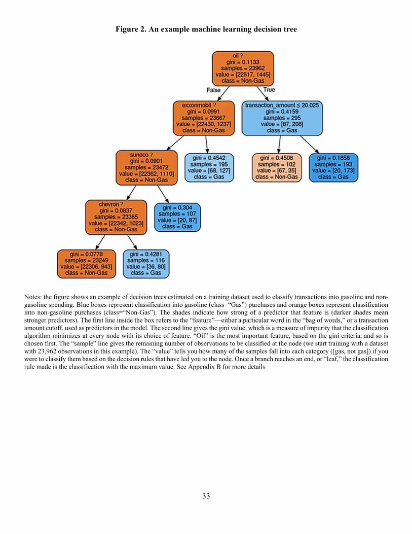
33

Figure 2. An example machine learning decision tree

Notes: the figure shows an example of decision trees estimated on a training dataset used to classify transactions into gasoline and non-gasoline spending. Blue boxes represent classification into gasoline (class=“Gas”) purchases and orange boxes represent classification into non-gasoline purchases (class=“Non-Gas”). The shades indicate how strong of a predictor that feature is (darker shades mean stronger predictors). The first line inside the box refers to the “feature”—either a particular word in the “bag of words,” or a transaction amount cutoff, used as predictors in the model. The second line gives the gini value, which is a measure of impurity that the classification algorithm minimizes at every node with its choice of feature. “Oil” is the most important feature, based on the gini criteria, and so is chosen first. The “sample” line gives the remaining number of observations to be classified at the node (we start training with a dataset with 23,962 observations in this example). The “value” tells you how many of the samples fall into each category ([gas, not gas]) if you were to classify them based on the decision rules that have led you to the node. Once a branch reaches an end, or “leaf,” the classification rule made is the classification with the maximum value. See Appendix B for more details

34

Figure 3. Distribution of log gasoline spending: CEX Diary versus App

Notes: the figure shows the distribution of daily log spending on gasoline in the Diary segment of the Consumer Expenditure Survey (CEX) and in the app data. Gasoline spending in the app data is identified using machine learning (ML). App includes all transactions that ML identifies as purchases of gasoline. App>$10 includes transactions that ML identifies as purchases of gasoline and that are greater than $10. See text for further details.

0.5

11.

5D

ensi

ty

$5$10

$15$20

$25$30

$40$50

$60$100

$200

Amount of Daily Gasoline Purchases, Dollars, Log Scale

App

App>$10

CEX Diary Survey

35

Figure 4. Reported gasoline spending (monthly) Panel A. CEX Interview Survey

Panel B. App data

Panel C. App data excluding zero spending

Notes: the figure reports monthly spending on gasoline in the Interview segment of the Consumer Expenditure Survey (CEX) and in the app data. The horizontal axis is in dollars. The size of the bin in is set to $1 in all panels.

0.0

5.1

.15

Den

sity

0 100 200 300 400 500Dollars per month

0.0

5.1

.15

.2D

en

sity

0 100 200 300 400 500Dollars per month

0.0

05

.01

.01

5D

ensi

ty

0 100 200 300 400 500Dollars per month

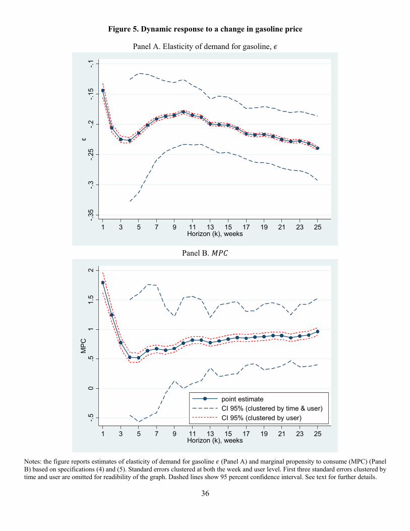
36

Figure 5. Dynamic response to a change in gasoline price

Panel A. Elasticity of demand for gasoline,

Panel B.

Notes: the figure reports estimates of elasticity of demand for gasoline (Panel A) and marginal propensity to consume (MPC) (Panel B) based on specifications (4) and (5). Standard errors clustered at both the week and user level. First three standard errors clustered by time and user are omitted for readibility of the graph. Dashed lines show 95 percent confidence interval. See text for further details.

-.35

-.3

-.25

-.2

-.15

-.1

ε

1 3 5 7 9 11 13 15 17 19 21 23 25Horizon (k), weeks

-.5

0.5

11.

52

MP

C

1 3 5 7 9 11 13 15 17 19 21 23 25Horizon (k), weeks

point estimateCI 95% (clustered by time & user)

CI 95% (clustered by user)

37

Table 1. Largest monthly changes in oil and gasoline prices

Largest Decreases Largest Increases

Date Percent Change Date Percent Change

Oil Gas Oil Gas 1986:2 -33 -6 1974:1 135 2008:12 -28 -21 1990:8 47 10 2008:10 -26 -14 1986:8 30 -5 2008:11 -25 -32 1948:1 24 2014:12 -22 -11 1990:9 23 9 2015:1 -20 -18 2009:3 23 1

Notes: Table shows the month-to-month percent change in West Texas Intermediate spot oil prices (FRED series OILPRICE and MCOILWTICO) and the corresponding change in average monthly regular gasoline prices, when available, from January 1946 – February 2016. For gasoline prices, the table use the BLS U.S. city average (BLS series APU000074714), since it is available further back in time than other available gasoline price data.

38

Table 2. Comparison of spending in the CEX and app data, 2013

Frequency and type of spending Moment

Mean St. Dev. Median Interquartile range

Panel A. Biweekly Spending on gas, dollars

CEX Diary Survey 84.72 83.42 65.00 101.44 App 87.83 98.79 58.03 130.87

Spending on non-gasoline items, dollars CEX Diary Survey 1,283.36 1,470.93 790.56 1,380.66 App 1,561.38 1,784.67 1,084.38 1,519.75

Ratio of gasoline to non-gasoline spending CEX Diary Survey 0.15 0.25 0.06 0.14 App 0.09 0.15 0.04 0.11

Panel B. Quarterly

Spending on gasoline, dollars CEX Interview Survey 646.63 530.87 540.00 630.00 App 627.94 588.24 475.33 660.18

Spending on non-gasoline items, dollars CEX Interview Survey 10,143.78 8,141.67 7,728.70 7,406.49 App 11,264.85 11,391.42 8,392.24 8,605.46

Ratio of gasoline to non-gasoline spending CEX Interview Survey 0.08 0.07 0.06 0.08 App 0.07 0.07 0.05 0.07

Notes: Means and standard deviation are from the distribution winsorized at the 1% level. The variables from the CEX use population sample weights. For Panel A, the ratio for a consumer/household is calculated as average value of the sum all gasoline spending during a biweekly period in 2013 divided by total non-gasoline spending in the corresponding biweekly period in 2013. For the app data, we mimic the design of the CEX Diary Survey by randomly drawing a two-week period for each user and discarding data for other weeks. For Panel B, the ratio for a consumer/household is calculated as the sum of all gasoline spending in a quarter, divided by total non-gasoline spending in that quarter.

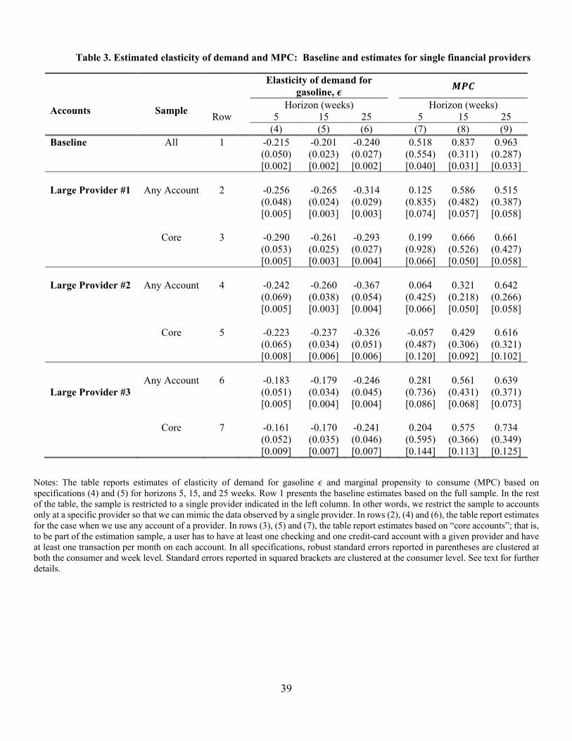
39

Table 3. Estimated elasticity of demand and MPC: Baseline and estimates for single financial providers

Accounts

Sample

Elasticity of demand for gasoline,

Horizon (weeks) Horizon (weeks) Row 5 15 25 5 15 25

(4) (5) (6) (7) (8) (9) Baseline All 1 -0.215 -0.201 -0.240 0.518 0.837 0.963 (0.050) (0.023) (0.027) (0.554) (0.311) (0.287) [0.002] [0.002] [0.002] [0.040] [0.031] [0.033] Large Provider #1 Any Account 2 -0.256 -0.265 -0.314 0.125 0.586 0.515 (0.048) (0.024) (0.029) (0.835) (0.482) (0.387) [0.005] [0.003] [0.003] [0.074] [0.057] [0.058] Core 3 -0.290 -0.261 -0.293 0.199 0.666 0.661 (0.053) (0.025) (0.027) (0.928) (0.526) (0.427) [0.005] [0.003] [0.004] [0.066] [0.050] [0.058] Large Provider #2 Any Account 4 -0.242 -0.260 -0.367 0.064 0.321 0.642 (0.069) (0.038) (0.054) (0.425) (0.218) (0.266) [0.005] [0.003] [0.004] [0.066] [0.050] [0.058] Core 5 -0.223 -0.237 -0.326 -0.057 0.429 0.616 (0.065) (0.034) (0.051) (0.487) (0.306) (0.321) [0.008] [0.006] [0.006] [0.120] [0.092] [0.102] Any Account 6 -0.183 -0.179 -0.246 0.281 0.561 0.639 Large Provider #3 (0.051) (0.034) (0.045) (0.736) (0.431) (0.371) [0.005] [0.004] [0.004] [0.086] [0.068] [0.073] Core 7 -0.161 -0.170 -0.241 0.204 0.575 0.734 (0.052) (0.035) (0.046) (0.595) (0.366) (0.349) [0.009] [0.007] [0.007] [0.144] [0.113] [0.125]

Notes: The table reports estimates of elasticity of demand for gasoline and marginal propensity to consume (MPC) based on specifications (4) and (5) for horizons 5, 15, and 25 weeks. Row 1 presents the baseline estimates based on the full sample. In the rest of the table, the sample is restricted to a single provider indicated in the left column. In other words, we restrict the sample to accounts only at a specific provider so that we can mimic the data observed by a single provider. In rows (2), (4) and (6), the table report estimates for the case when we use any account of a provider. In rows (3), (5) and (7), the table report estimates based on “core accounts”; that is, to be part of the estimation sample, a user has to have at least one checking and one credit-card account with a given provider and have at least one transaction per month on each account. In all specifications, robust standard errors reported in parentheses are clustered at both the consumer and week level. Standard errors reported in squared brackets are clustered at the consumer level. See text for further details.

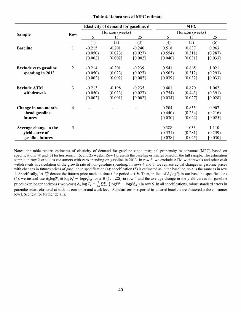
40

Table 4. Robustness of MPC estimate

Sample Row

Elasticity of demand for gasoline, Horizon (weeks) Horizon (weeks)

5 15 25 5 15 25 (1) (2) (3) (4) (5) (6)

Baseline 1 -0.215 -0.201 -0.240 0.518 0.837 0.963 (0.050) (0.023) (0.027) (0.554) (0.311) (0.287) [0.002] [0.002] [0.002] [0.040] [0.031] [0.033] Exclude zero gasoline

spending in 2013 2 -0.214 -0.201 -0.239 0.541 0.865 1.021 (0.050) (0.023) (0.027) (0.563) (0.312) (0.293)

[0.002] [0.002] [0.002] [0.039] [0.032] [0.033] Exclude ATM

withdrawals 3 -0.213

(0.050) -0.198 (0.023)

-0.235 (0.027)

0.401 (0.754)

0.870 (0.443)

1.062 (0.391)

[0.002] [0.001] [0.002] [0.034] [0.027] [0.028]

Change in one-month- ahead gasoline futures

4 - - - 0.204 0.855 0.907 (0.440) (0.234) (0.216) [0.030] [0.022] [0.025]

Average change in the

yield curve of gasoline futures

5 - - - 0.388 1.033 1.110 (0.531) (0.281) (0.259) [0.038] [0.025] [0.030]

Notes: the table reports estimates of elasticity of demand for gasoline and marginal propensity to consume (MPC) based on specifications (4) and (5) for horizons 5, 15, and 25 weeks. Row 1 presents the baseline estimates based on the full sample. The estimation sample in row 2 excludes consumers with zero spending on gasoline in 2013. In row 3, we exclude ATM withdrawals and other cash withdrawals in calculation of the growth rate of non-gasoline spending. In rows 4 and 5, we replace actual changes in gasoline prices with changes in futures prices of gasoline in specification (4); specification (5) is estimated as in the baseline, so is the same as in row 1. Specifically, let denote the futures price made at time for period . Then, in lieu of Δ log in our baseline specifications (4), we instead use Δ log ≡ log log for ∈ 1,… ,25 in row 4 and the average change in the yield curves for gasoline prices over longer horizons (two years) Δ log ≡ ∑ log log in row 5. In all specifications, robust standard errors in parentheses are clustered at both the consumer and week level. Standard errors reported in squared brackets are clustered at the consumer level. See text for further details.

41

Table 5. Elasticity of demand for gasoline and MPC: Consumer Expenditure Survey (CEX) versus App

Data and Sample Row

Elasticity of demand for gasoline,

Horizon (quarters) Horizon (quarters) 1 2 3 1 2 3 (1) (2) (3) (4) (5) (6)

Panel A: App data (quarterly)

Baseline 1 -0.084 -0.126 -0.383 1.000 1.050 2.320 (0.118) (0.110) (0.157) (0.478) (0.627) (0.797) [0.003] [0.003] [0.004] [0.030] [0.030] [0.050] CEX sample design

2 0.005 (0.073)

-0.111 (0.066)

-0.432 (0.057)

0.732 (0.548)

1.574 (0.287)

4.942 (1.017)

[0.006] [0.007] [0.011] [0.093] [0.162] [0.445]

Panel B: CEX

1980-2014 3 -0.429 -0.330 -0.352 -0.917 -0.526 -1.929 (0.041) (0.027) (0.027) (0.659) (0.638) (1.265) [0.010] [0.009] [0.012] [0.227] [0.178] [0.266]

1985-1987 4 -0.478 -0.396 -0.449 9.624 5.074 4.116 (0.168) (0.145) (0.090) (5.959) (4.057) (4.031) [0.067] [0.062] [0.064] [2.140] [1.380] [1.533] 1990-1992 5 -0.636 -0.562 -0.512 -6.420 -3.005 -4.917 (0.136) (0.142) (0.106) (4.775) (4.516) (6.450) [0.055] [0.051] [0.067] [2.210] [1.790] [2.450] 2014-2015 6 -0.431 -0.408 -0.447 1.384 2.020 6.895 (0.084) (0.043) (0.074) (1.407) (1.568) (2.306)

      [0.046] [0.042] [0.063] [1.008] [0.908] [1.487] Notes: the table reports estimates of elasticity of demand for gasoline and marginal propensity to consume (MPC) based on specifications (4) and (5) for horizons 1, 2, and 3 quarters. The CEX estimates use the ratio of gasoline spending to non-gasoline spending calculated in the first interview, and exclude this period from estimation. For the baseline estimates in Row 1, we use the same 2013 ratio of gasoline spending to non-gasoline spending as in the baseline estimates, and aggregate the spending and gasoline prices to the quarterly level. In row 2, we replicate the CEX sampling scheme, randomly selecting a start month for a user and keeping only the data for the 12 month period that follows it (if a full 12 months of data follow). We similarly use the non-gasoline consumption calculated in the first quarter, and exclude this period from the estimation. In all specifications, robust standard errors in parentheses are clustered at both the consumer and week level. Standard errors reported in squared brackets are clustered at the consumer level. See text for further details.

42

Table 6. MPC by liquidity status.

Measure of Hand-to-mouth consumers (HtM)

Elasticity of demand for gasoline,

Horizon (weeks) Horizon (weeks) 5 15 25 5 15 25

(1) (2) (3) (4) (5) (6) Panel A. Lagged HtM

Non-HtM -0.191 -0.155 -0.179 0.569 0.894 0.660 (0.057) (0.025) (0.026) (0.749) (0.438) (0.356)

[0.004] [0.003] [0.003] [0.087] [0.060] [0.058] HtM -0.239 -0.240 -0.293 0.547 1.044 0.896

(0.058) (0.030) (0.031) (0.829) (0.472) (0.471) [0.016] [0.010] [0.009] [0.297] [0.186] [0.181]

P-value (Non-HtM=HtM) 0.052 0.000 0.000 0.915 0.883 0.658 [0.003] [0.000] [0.000] [0.857] [0.779] [0.408] Panel B. Average HtM in 2013

Non-HtM -0.186 -0.164 -0.199 0.618 0.776 0.783 (0.054) (0.024) (0.027) (0.619) (0.311) (0.299) [0.003] [0.002] [0.002] [0.053] [0.043] [0.045]

HtM -0.274 -0.317 -0.373 0.742 1.336 1.383 (0.055) (0.030) (0.035) (0.838) (0.537) (0.428)

[0.007] [0.005] [0.005] [0.098] [0.088] [0.098] P-value (Non-HtM=HtM) 0.007 0.000 0.000 0.932 0.073 0.077

[0.000] [0.000] [0.000] [0.653] [0.000] [0.000] Panel C. Modal HtM in 2013

Non-HtM -0.191 -0.172 -0.209 0.597 0.899 0.893 (0.053) (0.024) (0.027) (0.651) (0.358) (0.320) [0.003] [0.002] [0.002] [0.052] [0.042] [0.044]

HtM -0.255 -0.287 -0.340 0.896 0.851 0.965 (0.053) (0.028) (0.032) (0.546) (0.270) (0.291)

[0.006] [0.004] [0.004] [0.106] [0.092] [0.099] P-value (Non-HtM=HtM) 0.012 0.000 0.000 0.579 0.410 0.641

[0.000] [0.000] [0.000] [0.007] [0.095] [0.382] Panel D. Extreme HtM in 2013

Non-HtM -0.195 -0.182 -0.221 0.613 0.924 0.933 (0.053) (0.024) (0.028) (0.639) (0.355) (0.319) [0.003] [0.002] [0.002] [0.049] [0.040] [0.042]

HtM -0.284 -0.318 -0.365 1.029 0.912 1.064 (0.056) (0.029) (0.033) (0.571) (0.297) (0.310)

[0.009] [0.006] [0.006] [0.156] [0.136] [0.146] P-value (Non-HtM=HtM) 0.002 0.000 0.000 0.470 0.472 0.753 [0.000] [0.000] [0.000] [0.001] [0.230] [0.626]

Notes: the table reports estimates of and based on equations (6)-(7) over periods, where is shown in the top row of the table. is the ratio of gasoline spending to non-gasoline spending for 2013 for consumer i. The title of each panel indicates how the presence/intensity of liquidity constraints is measured. Denote the dummy variable identifying hand-to-mouth consumers for a given month with ∗ . Panel A uses a dummy variable equal to one if a consumer is liquidity constrained in period 1 (recall that Δ operator calculates the growth rate between periods and ), i.e. ≡ ,

∗ . For other panels, we construct three measures on the 2013 sample which is not used in the estimation of and : the average value of ∗ (this continuous variable provides a sense of frequency of liquidity constraints; we denote this measure with , ), the modal value of ∗ (most frequent value; we denote this measure with , ), or the minimum value of ,

∗ during the 2013 part of the sample. The latter measure, which we denote with , and refer to as “extreme,” is equal to one only if a consumer is identified as hand-to-mouth in every month in 2013. Robust standard errors in parentheses are clustered by week and consumer. Standard errors reported in squared brackets are clustered at the consumer level. P-value (Non-HtM=HtM) is the p-value for the test of HtM and non-HtM responses being equal. See text for further details.

1

Online appendix for

THE RESPONSE OF CONSUMER SPENDING TO CHANGES IN GASOLINE PRICES*

Michael Gelmana, Yuriy Gorodnichenkob,c, Shachar Karivb, Dmitri Koustasb,

Matthew D. Shapiroc,d, Dan Silvermanc,e, and Steven Tadelisb,c

2

Appendix A: Construction of spending in the app data

This appendix discusses the data and provides details on how we prepare the data for statistical

analyses.

We received anonymized data directly from the personal financial management service

provider (app). The process by which the company acquires the data can differ across users,

account providers (e.g., Bank of America, Wells Fargo) and time. For some account providers, the

data are scraped from the website of an account provider, and in other cases a direct feed is received

from the account provider. All account numbers and other personal identifying information is

removed by the app company before we receive the data. Otherwise, we receive the data exactly

as it is received by the app. The table below summarizes the key variables in the data that are used

in our analysis: User_id - Anonymous identifier constructed by the personal

financial management service Posted_date - Date a transaction was recorded

Account_Provider_Id - An identifier for a specific account provider (e.g. Bank of America)

Account_Type - An indicator for whether an account is a checking account, savings account, credit card, or other account.

Transaction_Amount - The amount of the transaction

Is_Credit - Whether the transaction was a credit or a debit

Transaction_Description - A string variable describing the transaction.

Our cleaning processes proceeds in steps outlined below:

I. Remove likely duplicates +/- 3 days

Because the data may include pending transactions, a given spending may show up multiple times

in different transactions. For instance, if a transaction was pending on one day, and posted the

next day, we could see a duplicate recording of the same transaction in the data, which would not

reflect actual spending.

Some account providers indicate whether a transaction is pending or posted, and we first

remove all transactions that are flagged as pending, or contain the word “pending” in the

transaction string. Since many account providers do not indicate whether a transaction is pending,

and since this information also varies across time, we deal with this problem by removing

transactions that are duplicates on the dimensions of {User_Id, Account_Provider_Id,

3

Account_Type, Is_Credit, Transaction_Amount, Transaction_Description} over a 3 day window.

This removes approximately 5% of transactions. Some of these transactions could be non-

duplicates (for instance, if someone buys the exact same item every day), and so these transactions

will also be removed by this procedure. Using the data with likely duplicates removed, we next

proceed to calculate total spending and total income, which we aggregate to the weekly level.

II. Construct variables used in analysis and aggregate to weekly level

The transactions contain every single inflow and outflow from a household’s account, some of

which are not “consumption.” Two problematic types of transactions are transfers across accounts

and credit card payments. In most cases, transfers across accounts can be identified from the

transaction strings, since they are commonly flagged as “transfer,” “xfer,” “tfr,” “xfr” or “trnsfr.”

We remove all transactions with these words appearing in their description.

Credit card payments reflect lagged spending that we have already included in our measure

of total spending, since we can see the individual purchases that make up the credit card payment

on the credit card. Therefore, we wish to identify and remove these payments. We identify credit

card payments as debits appearing on a non-credit-card account that also appears as a credit to a

credit card, and remove these.

We also remove the largest transaction greater than $1,000 in a weekly window, since these

transactions appear to be predominantly credit card payments and transfers missed by our

procedure. As a caveat, this likely also removes mortgage payments (committed spending),

extremely large durables purchases (such as a down payment on a car, although we would still see

car payments), and payments on tax liabilities. To summarize, our measure of “total spending”

used in this paper is defined as:

{Total spending} = {Total Account Debits} – {Flagged Duplicates} – {Transfers} –

{Credit Card Payments} – {Largest Transaction > $1,000 (if any)}.

4

Appendix B: Machine Learning Classification of Transactions

As discussed in Appendix 1, the data we receive contain raw transaction strings. These transaction

strings differ across account providers in their context. We wish to identify spending that comes

from gasoline. Identifying to which of a set of categories an observation belongs, based on

information in the transaction descriptions, is a classic “classification” problem in machine

learning.

We seek a simple machine learning (ML) model to identify gasoline spending in the data.

For this to work, we require a “training” set of data containing observations whose category

membership is known. Fortunately, two account providers in our data categorize the transactions

into merchant category codes (MCCs) directly in the transaction strings. These two cards represent

about 3% of all transactions. As discussed in the text, it is virtually impossible to separate out our

main MCC of interest, 5541, “Automated Fuel Dispensers” from MCC code 5542, “Service

Stations,” which in practice covers gasoline stations with convenience stores.1 Because

distinguishing gasoline purchases classified as 5542 or 5541 is nearly impossible with the

information in transaction descriptions,2 we group transactions with these two codes together.

Before proceeding with the details of the machine learning model, it is useful to discuss an

alternative approach that identifies all gasoline stations in the data through string matching

techniques. To see why this is infeasible, consider that the 100 most popular gasoline station

strings cover approximately 50% of the total market share in the transactions where we know the

MCC codes. Scaling up is costly: to get 90 percent of the market share, we would need to search

for over 30,000 strings (Appendix Figure 1). Moreover, since other spending can often have similar

transaction descriptions, it is hard to know what strings minimize noise while maximizing

predictive power. The machine learning algorithm thus helps discipline the approach of what

transaction strings contain the most useful information. The machine learning procedure proceeds

in 3 steps: training, testing, and application.

Machine learning requires both a “training” data set—data actually used to fit a

classification model-—and a “testing” data set to evaluate the out of sample performance of the

model. In the training step, we build a prediction model using data with the MCC codes (i.e. data

1 To be clear, “Service Stations” do not include services such as auto repairs, motor oil change, etc. 2 E.g., a transaction string with word “Chevron” or “Exxon” could be classified as either MCC 5541 or MCC 5542.

5

where classification is known). We use the larger of the two account providers as the training data

set, and test the performance of the model on the smaller account. We explicitly set aside the

second card as the training data set because transaction strings, which we will feed into the model

to classify the data, can differ across account providers. Therefore, if we train on data from the two

accounts, we may fit our two cards extremely well, but we may have a poor “out of sample” fit of

our model.

The classification algorithm we use is known as a random forest classifier, which fits a

number of separate decision trees. A decision tree is a series of classification rules that ultimately

lead to a classification of a purchase as gasoline or not. The rules, determined by the algorithm,

minimizes the decrease in accuracy when a particular model “feature” is removed. The features

we use are the transaction values and individual words in the transaction strings (this approach is

known as “bag of words”), after some basic string cleaning. We limit the number of features to

20,000 words, and transaction amounts rounded to the nearest 50 cents. An example decision tree

is shown in Appendix Figure 2.

In this example, the most important single word is “oil.” If a transaction string contains

the word oil, the classification rule is to move to the right, otherwise the rule is to move to the left.

If the string does not contain the word oil, the next most important single word is “exxonmobil.”

The tree keeps going until all the data are classified.

Whether a transaction is classified as gasoline spending or not is simply the majority vote

over a number of decision trees. This is known as a “white box algorithm” because the model

determines optimal decision rules that we can see. We use prebuilt packages from the python

machine learning toolkit.3

The results of the model are shown in Appendix Table B.1. The model predicts

292,997/(292,997+26,553) = 92% of automated fuel dispenser and service station transactions.

The ratio of misclassfications to correct classifications is (30,080+26,553)/292,997=19%.

In summary, the ML approach is able to correctly classify over 90% of gasoline spending

in the test data. If a human were to do this, she would need to identify over 30,000 strings. In

3 Scikit-learn: Machine Learning in Python, Pedregosa et al., JMLR 12, pp. 2825-2830, 2011.

6

addition, the model correctly classifies over 99.5% of the gasoline stations that would have been

captured in an alternative approach of identifying the 100 largest gasoline stations by market share.

Appendix Figure B.1

0.2

.4.6

.81

Cum

ula

tive

Sha

re o

f A

ll A

FD

Tra

nsac

tions

0 10000 20000 30000 40000Number of gas stations, ranked by number of transactions

Cumulative Market Share

7

Appendix Table B.1. Confusion Matrix

Actual gasoline spending

No Yes

Pre

dic

ted

ga

soli

ne

spen

din

g

No 2,741,524 26,553

Yes 30,080 292,997

Notes: Table shows the four possible outcomes for our testing data set which is not used in any way to train the model, as described in the text. The rows “Predicted gasoline spending” refer to the binary prediction from the model as not gasoline, “no,” or gasoline, “yes”. Actual gasoline refers to the “truth,” which is known for the case of our testing dataset.

8

Appendix C. Additional Tables and Figures

Appendix Figure C.1. Distribution of Ratio of Gasoline to Non-Gasoline Spending, 2013Q1-2014Q4

Note: the figure shows the quarterly gasoline to non-gasoline spending distribution in the app data and the CEX interview survey (solid lines), and the same ratio calculated over all of 2013 (dashed lines).

05

1015

20D

ensi

ty

0 .1 .2 .3Share

App Gas Ratio (All) Gas Ratio (2013)

CEX Interview Survey Gas Ratio (All) Gas Ratio (2013)

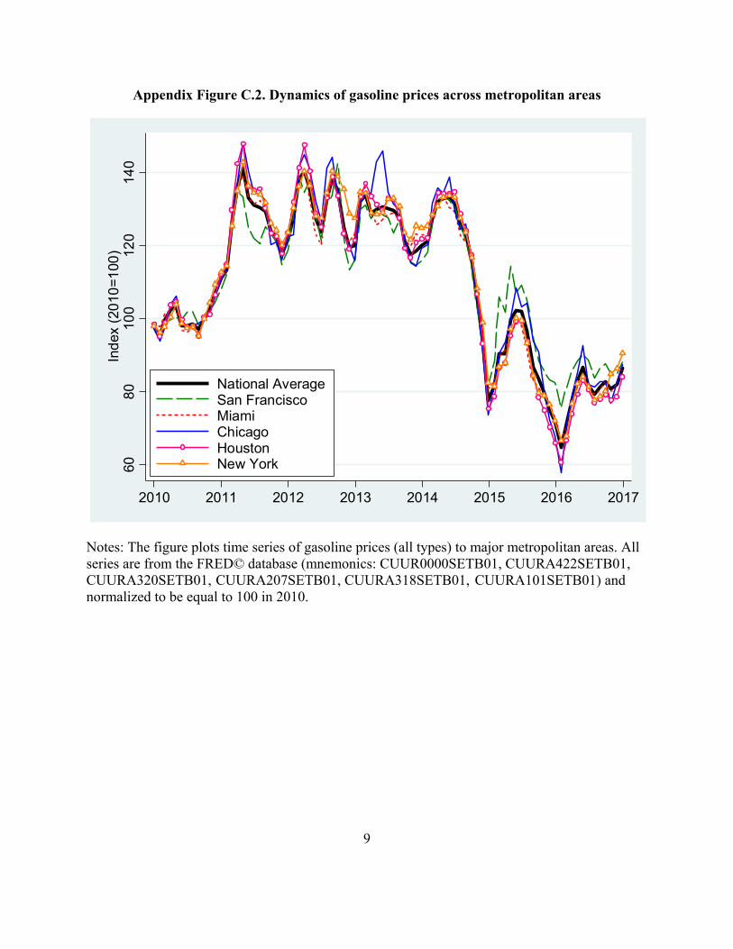
9

Appendix Figure C.2. Dynamics of gasoline prices across metropolitan areas

Notes: The figure plots time series of gasoline prices (all types) to major metropolitan areas. All series are from the FRED© database (mnemonics: CUUR0000SETB01, CUURA422SETB01, CUURA320SETB01, CUURA207SETB01, CUURA318SETB01, CUURA101SETB01) and normalized to be equal to 100 in 2010.

6080

100

120

140

Ind

ex (

2010

=1

00)

2010 2011 2012 2013 2014 2015 2016 2017

National AverageSan FranciscoMiamiChicagoHoustonNew York

10

Appendix Table C.2. Gelman et al. (2014)

Source: Gelman et al. (2014)

11

Appendix D: Marginal Propensity to Consumer in Partial Equilibrium versus General

Equilibrium Effects

In this appendix, we link the marginal propensity to consume (MPC) to structural parameters and explore how partial equilibrium MPC is potentially related to general equilibrium effect of gasoline price changes. In this exercise, we vary the price of gasoline holding everything else constant. Partial equilibrium Consumer a household that solves the following problem

max . .

where is the numeraire good (or “non-gasoline spending”; we normalize 1), is “gasoline”, is labor, is wages, and functions , , describe how the household values goods and leisure. In a popular case, so that the utility is quasi-linear. Because this is a partial equilibrium model, we take wages as given.

The first-order conditions yield:

After log-linearization of these FOCs and the budget constraint, we have (assume is fixed)

′

1

where ≡ and 1 and is the Frisch labor supply elasticity,

≡ 0 and ≡ 0. Note that the first two conditions imply that

. It follows that

1 1 1

1 1

1 1 ⇒

1

11

1

11

11 ⇒

12

1

11

11

where 1 is estimated from the regressing on . Note that this equation provides structural interpretation of our specification (2) in the paper. We know from the derivation above that

1

1

11

1

1 11

11

So that 1 0. Also note that 1 1 .

Hence, marginal propensity to consume (MPC) is equal to 1

11

1

1

11

11

1 11

1

11

0

In the case of quasi-linear utility, ∞ and 1. General equilibrium In the general equilibrium version of the model, we consider two sectors. The first sector (sector A) produces consumer goods. The second sector (sector B) produces gasoline. Gasoline is consumed by households working in both sectors. Gasoline is also a production input in the first sector. We assume that households cannot move across sectors, which is likely a reasonable approximation in the short-to-medium run. The mass of households in sector A is . The mass of households in sector B is 1 . The economy is closed. Households in sector A solve the following maximization problem:

max . .

13

where is the numeraire good (or “non-gasoline spending”; we normalize 1), is “gasoline”, is labor, is wages. After log-linearization of first-order conditions and the budget constraint, we have

′

1

where ≡ and 1 and is the Frisch labor supply

elasticity, ≡ 0 and ≡ 0. Note that the first two conditions imply that

. Households in sector B solve the following maximization problem:

max . .

After log-linearization of first-order conditions and the budget constraint, we have

′

1

where ≡ and 1 and is the Frisch labor supply

elasticity, ≡ 0 and ≡ 0. Note that the first two conditions imply that

. Production in sector A is characterized by constant return to scale and perfect competition:

⇒ 1 where is gasoline used in production of good 1. Perfect competition means . Given normalization 1, we have 1. Given the Cobb-Douglass production function, we find that 1 . This means that

1 .

14

Production in sector B is also characterized by constant return to scale (production function is linear in labor) and perfect competition:

⇒ ⇒

Market clearing in sector A:

1 ⇒ 1

Market clearing in sector B:

1 ⇒ 1

where is the total amount of oil consumed in production of good 1 (each firm in this sector consumes and is the mass of firms in the sector). Now we derive MPC for each group of households:

1 1 1 1

11

Clearly, 0.

1 1 1

1

We can generate 0 if demand for good “1” is sufficiently elastic (i.e., 1), which

seems a reasonable assumption. With utility quasi-linear , we have . The sensitivity of group A’s total spending on gasoline to the price of gasoline is

1 1

11 1

1

Hence, 1 .

The MPC we define in the paper is

15

1 1 1 1

11

1 1 1 1

11

11

11

That is,

1 1 1 1

11

11

1

1 1 11

1

1 11

1 11

1 1 11

1

11 1

11

For comparison, in the partial equilibrium model (effectively 1) we had 1

11

1

Note that the general equilibrium MPC for this group is greater than the partial equilibrium MPC because 0 and 0 (provided 1).

Doing a similar derivation for group B, we find that

1 1 1

1

Note that increases in . Employment for these agents increases in response to a shock in if their demand for good “1” is sufficiently elastic:

11

With utility quasi-linear in (i.e., ∞) , we have . Now the sensitivity of group B’s total spending on gasoline to the price of gasoline is

16

1 1 1 1

1

11

1 11

1

Hence,

1 11

1 11

11

It follows that MPC for type B is

1 11

1

1 11 1

1

The denominator is positive ( 1). The numerator is positive too ( 1). Thus, this MPC is negative and can be greater than one in absolute magnitude. For example, with infinitely elastic demand for good “1” (i.e., quasi-linear utility in ), we have

1 11

1 0

which can be less than -1 provided that the share good “2” in the consumption basket of type B agent is sufficiently small. The aggregate employment depends on the relative strength of employment responses across sectors:

1 For the case with quasi-linear utility, we have and . Output is likely to decrease in response to a hike in oil prices. First, one can proxy inelastic supply of gasoline with inelastic supply of labor, that is 0 and hence (which has a clear sign) drives aggregate employment. Second, 1 is small and, thus, it would take very large employment effects in sector 2 to drive aggregate employment. The aggregate 1 . Note that and have different signs. Depending on parameter values, partial equilibrium MPC can be greater or smaller than the aggregate .