THE REVERSIBILITY OF THE ADSORPTION OF METHANE-METHYL

MERCAPTAN MIXTURES IN NANOPOROUS CARBON

A Thesis presented to

the Faculty of the Graduate School

University of Missouri

In Partial Fulfillment

of the Requirements for the Degree

Master of Physics

by

MONIKA R. GOŁĘBIOWSKA

Dr. Carlos Wexler, Thesis Supervisor

MAY 2011

The undersigned, appointed by the Dean of the Graduate School, have examined the thesis entitled

THE REVERSIBILITY OF THE ADSORPTION OF METHANE-METHYL

MERCAPTAN MIXTURES IN NANOPOROUS CARBON

presented by Monika R. Gołębiowska

a candidate for the degree of Master of Physics, and hereby certify that in their opinion it is worthy of acceptance. ________________________________ Dr. Carlos Wexler, Thesis Supervisor Department of Physics and Astronomy, University of Missouri, Columbia ________________________________ Dr. Peter Pfeifer Department of Physics and Astronomy, University of Missouri, Columbia ________________________________ Dr. Michael Roth Department of Physics, University of Northern Iowa, Cedar Falls

ii

ACKNOWLEDGEMENTS

First, I would like to thank Carlos Wexler for enlightening discussions and lots of ideas.

His advice and contribution to my work have been very important. I would like to thank

him for allowing me to develop the kind of confidence and character traits which will

allow me to pursue a successful research career.

Second, I would like to thank Michael Roth who has always been available for help and

strongly contributed to my understanding of Molecular Dynamics simulations. I am

grateful for his patience and continuous involvement.

I would like to thank Lucyna Firlej and Bogdan Kuchta for their support throughout the

duration of the project. They strongly contributed to my intellectual upbringing in

physics.

I would like to express my gratitude to Peter Pfeifer. His kindness and support have

been invaluable through the course of my apprenticeship.

The project was supported by Grant Number 500-08-022 from California Energy

Commission.

I have also been fortunate to be surrounded by colleagues and friends from ALL-CRAFT

group. I have benefited immensely from their knowledge throughout discussions and

collaborations on various research projects, and from the friendship which sustained me

throughout the years. Special thanks to Raina Olsen for companionship and assistance in

all aspects of life.

Some people come into our lives and quickly go. Some stay for awhile and leave

footprints… Thus, I would like to thank all the others I have met and who influenced me

because without them I might not be here.

Last but not least, I would like to thank my mother for her love, understanding and her

continual support in pursuing my dreams. She encouraged me to take the road which

led to where I am now. Dziękuję Ci, Mamo.

iii

Contents

List of Figures ...................................................................................................................... iv

List of Tables ....................................................................................................................... vi

1. Introduction .................................................................................................................... 1

2. Simulation method: Molecular Dynamics ...................................................................... 5

2.1. Initialization ............................................................................................................. 6

2.2. Force calculations .................................................................................................... 7

2.3. Verlet algorithm ....................................................................................................... 8

2.5. Periodic boundary conditions .................................................................................. 9

3. Simulation setup ........................................................................................................... 11

4. Choice of force field ...................................................................................................... 14

5. Results and discussion .................................................................................................. 24

5.1. Adsorption isotherms ............................................................................................ 24

5.2. Adsorption energy: maximum value and fluctuations, mobility .......................... 26

5.3. Diffusion in adsorbed methane-methyl mercaptan mixtures ............................... 30

5.3.1. Graphene surface ............................................................................................ 30

5.3.2. 0.7 nm slit-shaped pores................................................................................. 32

5.4. Required enhancement of mercaptan concentration in natural gas .................... 38

6. Summary and Conclusions ............................................................................................ 41

References ........................................................................................................................ 43

iv

List of Figures

Figure 1. Methane storage capacity per liter of adsorbent as a function of pressure. At pressure equal 3.5 MPa nearly 100 g of natural gas can be stored in a tank filled with adsorbent such as activated carbon. The same amount of condensed natural gas (CNG) can be stored in an empty tank at pressure about 17 MPa. .............................................. 2

Figure 2. Nanoporous material for vehicular applications-from corn cob to monolith in tank. [18] ............................................................................................................................. 3

Figure 3. Two-dimentional periodic domain showing unit cell (in the center of the scheme) and its images (surrounding replicas). ............................................................... 10

Figure 4. Side view of the 14.0 x 10.0 x 21.0 nm3 simulation box containing three graphene sheets (blue circles), methane (small green circles) and methyl mercaptan (larger, blue and yellow circles). The graphene sheets are 10.0 x 10.0 nm2, leaving space for a gas phase in equilibrium with the adsorbed phase. a) the initial placement of gas molecules beyond slit volume. b) Stabilized system. Periodic boundary conditions were used in all directions. ........................................................................................................ 12

Figure 5. a) Gas distribution on the edge of a typical slit. b) Corresponding density profile of molecules in x-direction (outside the slit, x < 2 nm). ................................................... 13

Figure 6. OPLS-UA representation of methane (left) and methyl mercaptan (right). .... 16

Figure 7. a) All Atom representation of methane: tripod down, tripod up and United Atom molecule, b) Comparison of the interaction energies between three representations. ................................................................................................................ 18

Figure 8. Comparison of methane–graphite interaction energy calculated using OPLS parameters with selected data available in literature: a) AA approach, b) UA approach............................................................................................................................................ 20

Figure 9. Energy of methane interaction with 1, 2, 3, and 4 layers of graphene: a) UA representation of methane, b) AA representation of methane (tripod down configuration). .................................................................................................................. 22

Figure 10. Snapshots of methyl mercaptan-methane mixture at 195 K (below its boiling point) and molar fractions of CH3SH equal a) 0.065, b) 0.019. Aggregation of mercaptans at the higher concentration is seen. For clarity only CH3SH molecules are shown. ............................................................................................................................... 23

Figure 11. Adsorption isotherms of methane-mercaptan mixtures in 0.7 nm slits at a) 195 K, b) 298 K, c) 320K. ................................................................................................... 25

v

Figure 12. Graphene-methane interaction energy vs. time step for various representative molecules. The variations in energy correspond to migrations between slits and edges, and to the gas phase. .............................................................................. 28

Figure 13. Graphene-mercaptan interaction energy vs. time step for various representative molecules. ................................................................................................ 29

Figure 14. Trajectories of a single methyl mercaptan on graphite surface. a) T = 195 K and p = 1.2 bar, b) T = 195 K and p = 24.8 bar, c) T = 298 K and p = 3.6 bar, d) T = 298 K and p = 69.7 bar. ............................................................................................................... 31

Figure 15. Typical trajectories of single methyl mercaptan in 0.7 nm slit Left: side view, right: top view. a) At T = 195 K, p = 21.5 bar an adsorption event and limited in-plane diffusion. b) At T = 298 K, p = 167 bar the adsorption/desorption events and both in-plane diffusion and out-of-plane movement. .................................................................. 33

Figure 16. Radial distribution functions of mercaptans in 0.7 nm slit at a) 195 K, b) 298 K, c) 320 K. ............................................................................................................................. 34

Figure 17. Two-dimensional mean square displacement as a function of simulation time plots for methane and methyl mercaptan at a) 195K, b) 298 K and c) 320 K. ................. 36

Figure 18. Diffusion coefficients vs. pressure at a) 195 K, b) 298 K and c) 320 K. ........... 37

vi

List of Tables

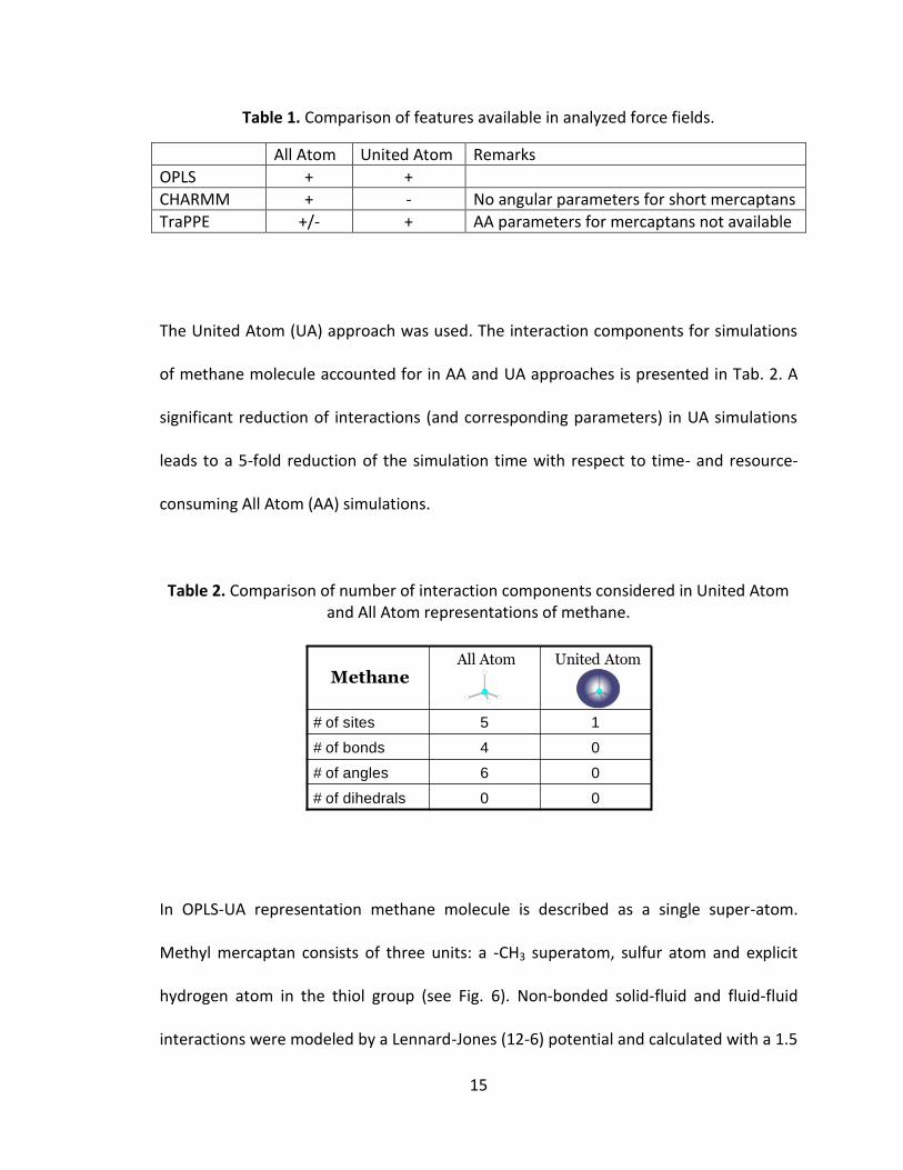
Table 1. Comparison of features available in analyzed force fields. ................................ 15

Table 2. Comparison of number of interaction components considered in United Atom and All Atom representations of methane. ...................................................................... 15

Table 3. The OPLS-UA force field non-bonded parameters in UA and AA approaches used in MD simulations. ................................................................................................... 17

Table 4. Energies of the strongest gas-substrate interactions. ....................................... 26

1

1. Introduction

Natural gas (NG) consists mainly of methane, which has hydrogen to carbon ratio higher

than any other molecule used as a primary fuel. Of all hydrocarbons NG has the highest

energy density per unit mass and the lowest carbon dioxide emission per unit energy,

making it an effective and relatively clean alternative for energy applications, especially

when considering its lower cost compared to gasoline. Unfortunately, the low density

of methane compared to liquid fuels makes its storage more difficult, requiring

compression at very high pressures (p ≥ 250 bar ≈ 3,600 psig, compressed NG, CNG) or

liquefaction at very low temperatures (T ≈ −162 °C, liquefied NG, LNG). Either

alternative increases significantly the cost of operation both in terms of production

(energy costs, equipment, safety) and storage (bulky tanks and/or cryogenics). In

particular, for the case of vehicular use, the use of CNG employs heavy bulky tanks,

significantly reducing the available cargo/passenger space.

A promising alternative is to store the fuel as adsorbed NG (ANG). This is possible

through physisorption of a gas into a suitable porous solid, designed to hold the fuel at

relatively low pressures (e.g., 35 bar ≈ 500 psig). Highly porous media have sufficient

volumetric storage ability to store NG at densities comparable to a high-pressure CNG

2

tank. The lower operational pressure allows thinner tank walls and a convenient shape

[6], resulting in potentially significant cost savings, improvements in safety and reduced

cargo volume loss. The difference between storage capacities of adsorbent filled tank

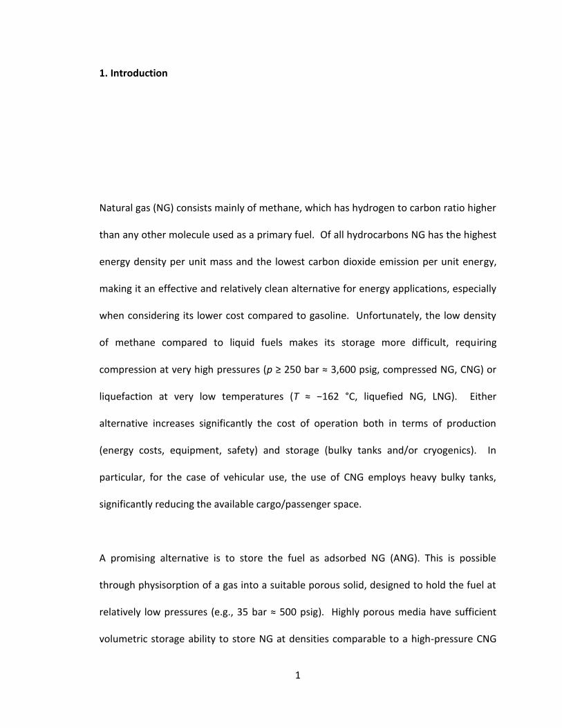
and empty tank is shown in Fig. 1.

Figure 1. Methane storage capacity per liter of adsorbent as a function of pressure. At

pressure equal 3.5 MPa nearly 100 g of natural gas can be stored in a tank filled with

adsorbent such as activated carbon. The same amount of condensed natural gas (CNG)

can be stored in an empty tank at pressure about 17 MPa.

Carbon-based nano-porous materials appear to be one of the most attractive

candidates for room temperature ANG storage for various reasons: (i) low-cost, (ii) no

toxicity, (iii) high availability; (iv) low weight; and (v) the fact that isosteric heats of

adsorption for methane in activated carbon is 18–20 kJ/mol (2,200–2,400 K) [15],[11],

very close to the “Optimum Conditions for Adsorptive Storage” of Bhatia and Myers [5].

3

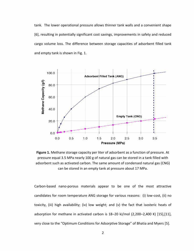
Some of the best performing carbons have been manufactured from organic wastes

such as corn cob, see Fig.2 [18], and a broad range of experimental methods have been

applied to characterize such materials (see [25] and references therein). Furthermore,

an understanding of the adsorption mechanism and kinetics at the microscopic level

comes from numerical simulations. Monte Carlo [10],[3] and Molecular Dynamics [9]

methods have been applied to analyze a wide range of aspects: isotherms of adsorption

[23], interaction energies [24],[2], methods of adsorbent structure approximations

[20],[7] and migration of gas molecules into and out of the slit volumes [17].

Figure 2. Nanoporous material for vehicular applications-from corn cob to monolith in

tank. [18]

4

Despite all the progress in understanding methane adsorption, very little has been done

to understand how other important components of NG act in an ANG setup. Since

methane (and other alkanes in NG) is flammable and potentially explosive, significant

safety considerations must be satisfied for common use. Methane is odorless therefore

it has to be odorized. Typically about 200 ppb of mercaptans are added. Such

concentration enables detection of gas in air when the concentration of NG reaches

1/5th of the lower explosive limit (5% by volume in air at 200C, see, e. g., [1]). To the

best of our knowledge there are no studies on mercaptans in the context of ANG

systems. On the contrary, most current studies of ANG systems are focused on

completely removing mercaptans from gas mixtures (e.g., by increasing mercaptan

captivation in chemically modified carbons [4]). It would seem inconceivable to us,

however, that a significant deployment of ANG could be achieved without the basic

safety mechanism of human detection of NG leaks from an ANG system. Therefore, in

this work we present a detailed computational effort of the behavior of methane-

mercaptan mixtures in nanoporous carbons. Our results indicate that although

mercaptans adsorb preferentially as compared to methane, they still are able to migrate

with relative ease within sub-nm pores, and that the adsorption is reversible. We

estimate that a modest increase in the concentration of mercaptans in NG (prior to

adsorption) will be sufficient to permit a desorbed phase to retain the amount of

mercaptans above the human detection threshold. Our conclusions further indicate

that mercaptans should not pose a major problem contaminating/clogging the

adsorbants, thus their use should be possible in ANG systems.

5

2. Simulation method: Molecular Dynamics

Molecular Dynamics (MD) simulations [21] provide a powerful tool for equilibrium

predictions of complex, multiatomic systems. Based on statistical mechanics this

computational approach gives the insight to dynamical processes which cannot be

calculated analytically and accounts for an important complementary technique to the

experimental measurements. The time-dependent evolution of the system, predicted by

MD simulations, provides outlook on the continuous motion (set of trajectories) of

molecules under investigation. Numerical data gathered during the calculations can be

used to derive macroscopic properties which can be compared to the experimental

measurements.

In order to run MD simulations there are several steps that have to be followed. First it

is required to initialize the system by setting an initial configuration (at time t = 0).

Initially, the energy of the system is minimized with respect to the molecular

coordinates; then the initial velocities are assigned and the dynamic equilibration of the

system begins. This means that the forces acting on the atoms are calculated (after

every time step) and each of the atoms follows Newton’s laws of motion. When the

energy of the system fluctuates about constant value throughout the simulations the

6

trajectories can be analyzed. The details on the main steps of MD simulations are given

in sections 2.1-2.4.

2.1. Initialization

In order to start the MD simulations it is necessary to set initial coordinates of particles,

which requires basic knowledge on molecular interactions and chemical bonding. When

the configuration is build, the program assigns the velocities to each atom so that the

total momentum equals zero, and the velocities are then rescaled to satisfy the

equipartition theorem, i.e. that the average kinetic energy per degree of freedom

follows

(1)

where v is a component of velocity of a given particle. During simulations of the system

consisting of N particles the total kinetic energy undergoes fluctuations, therefore its

average defines an instantaneous temperature:

(2)

7

In order to obtain the desired temperature at time t, the velocities are scaled by factor

[T/T(t)]1/2.

2.2. Force calculations

For each pair of atoms within a cutoff distance (dependent on the interaction potential

between them) the forces are calculated. This is the most time consuming part of the

simulations, since for system of N elements there are N*(N-1)/2 pair distances. The x-

component of the force:

(3)

If the Lennard-Jones potential is used the expression above becomes:

(4)

8

2.3. Verlet algorithm

The Verlet algorithm is used for the approximation of the positions of particles of

simulated system in the next time step. The popularity of the approach is mainly due to

its simplicity and the fact that it leads to a little long-term energy drift through the

simulations.

A Taylor expansion of the coordinate of a particle around time t:

(5)

(6)

Adding up these equation leads to:

(7)

or

(8)

The estimation of new positions thus has an error of the order Δt4, where Δt is the time

step.

9

At this point it is possible to obtain the velocities:

(9)

or

(10)

Moving the algorithm forward into the next time step, the current positions become old

ones and the new positions become current.

2.5. Periodic boundary conditions

In general, one is limited to simulation boxes of relatively small size. Unless surface

effects are of particular interest, periodic boundary conditions (PBC), in which there are

no edges, are used to better approximate the conditions in large systems. The total

energy of the computed system with PCB is calculated according to the equation (11)

(11)

10

where NM is the number of molecules at any periodic box, L is the lateral dimension of

the periodic box and stands for an arbitrary vector of 3 integer numbers, among which

the prime over the sum indicates that the term with i = j is to be excluded when = 0.

Of course, it is important to bear in mind the imposed artificial periodicity when

considering properties which are influenced by long-range correlations. Special

attention must be paid to the case where the potential range is not short: for example

for charged and dipolar systems.

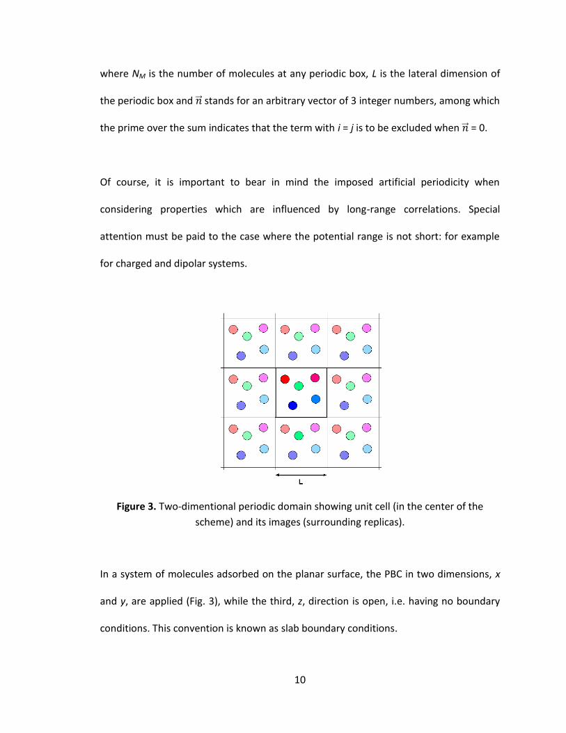
Figure 3. Two-dimentional periodic domain showing unit cell (in the center of the

scheme) and its images (surrounding replicas).

In a system of molecules adsorbed on the planar surface, the PBC in two dimensions, x

and y, are applied (Fig. 3), while the third, z, direction is open, i.e. having no boundary

conditions. This convention is known as slab boundary conditions.

11

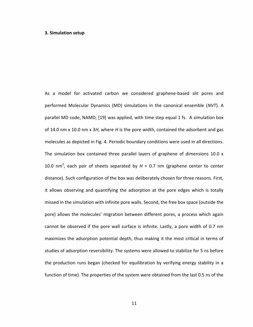
3. Simulation setup

As a model for activated carbon we considered graphene-based slit pores and

performed Molecular Dynamics (MD) simulations in the canonical ensemble (NVT). A

parallel MD code, NAMD, [19] was applied, with time step equal 1 fs. A simulation box

of 14.0 nm x 10.0 nm x 3H, where H is the pore width, contained the adsorbent and gas

molecules as depicted in Fig. 4. Periodic boundary conditions were used in all directions.

The simulation box contained three parallel layers of graphene of dimensions 10.0 x

10.0 nm2, each pair of sheets separated by H = 0.7 nm (graphene center to center

distance). Such configuration of the box was deliberately chosen for three reasons. First,

it allows observing and quantifying the adsorption at the pore edges which is totally

missed in the simulation with infinite pore walls. Second, the free box space (outside the

pore) allows the molecules’ migration between different pores, a process which again

cannot be observed if the pore wall surface is infinite. Lastly, a pore width of 0.7 nm

maximizes the adsorption potential depth, thus making it the most critical in terms of

studies of adsorption reversibility. The systems were allowed to stabilize for 5 ns before

the production runs began (checked for equilibration by verifying energy stability in a

function of time). The properties of the system were obtained from the last 0.5 ns of the

12

simulations. Since MD operates in the canonical ensemble the pressure of the gas must

be determined a posteriori for each run after equilibration is achieved.

a)

b)

Figure 4. Side view of the 14.0 x 10.0 x 21.0 nm3 simulation box containing three

graphene sheets (blue circles), methane (small green circles) and methyl mercaptan

(larger, blue and yellow circles). The graphene sheets are 10.0 x 10.0 nm2, leaving space

for a gas phase in equilibrium with the adsorbed phase. a) the initial placement of gas

molecules beyond slit volume. b) Stabilized system. Periodic boundary conditions were

used in all directions.

The simulations procedure is as follows: The initial configuration (Fig. 4. a.) consisted of

a random placement of methane and mercaptan molecules in the volume outside the

slits. Depending on pressure and temperature, the analyzed systems contained 1,836 to

2,550 (T = 195 K, dry ice temperature), 1,326 to 2,040 (T = 298 K, room temperature),

and 1,224 to 1,938 (T = 320 K) gas molecules in a constant proportion (98% methane,

2% methyl mercaptan). At energetic and conformational equilibrium (Fig. 4.b.) gas

0.0

2.1

z-d

irection

[nm

]

0.0 2.0 12.0 14.0

x-direction [nm]

0.0

2.1

z-d

irection [nm

]

0.0 2.0 12.0 14.0

x-direction [nm]

13

molecules adsorbed within slits and on the pores edges and some remained in gas

phase in the volume outside the slits. This is shown schematically in Fig. 5 (projection

along the y direction). The amount of adsorbed molecules was calculated from the

coordinates of molecules for each frame in the simulations. The adsorption isotherms

were calculated and averaged over the frames of the production runs. The analysis of

methane and mercaptan trajectories and gas-slit interaction energies were also

obtained from the last 0.5 ns of simulations. Pressures were obtained from the density

of molecules in the gas phase (i.e., x < 1 nm and x > 13 nm in Fig. 5) using the ideal gas

law.

a)

b)

Figure 5. a) Gas distribution on the edge of a typical slit. b) Corresponding density profile

of molecules in x-direction (outside the slit, x < 2 nm).

0.0 1.0 2.0

x-direction [nm]

0.0 0.5 1.0 1.5 2.0

Dis

trib

utio

n o

f C

H4 m

ole

cu

les

x-direction [nm]

14

4. Choice of force field

Several force fields (sets of interaction parameters) are available in literature. For

simulations presented in this chapter, the initial search through available

documentation focused on three most standard force fields: OPLS (Optimized Potentials

for Liquid Simulations) [12], CHARMM (Chemistry at HARvard Molecular Mechanics)[13],

and TraPPE (Transferable Potentials for Phase Equilibria)[14]. CHARMM was originally

parameterized to describe large biological systems such as proteins and lipids. The

description of small molecules, including mercaptans, is not precise and some of the

angular parameters are missing. Additionally, this force field does not provide data for

United Atom approach. TraPPE gives the United Atom parameters for most organic

compounds, but the All Atom description of heteroatomic systems has not been

developed. The OPLS force field contains all interaction parameters for both methane

and methyl mercaptan, in both AA and UA approaches; therefore it was chosen to

describe the interactions in our simulations. The schematic comparison of the

availability of interaction parameters for simulations of methane-metyl mercaptan

mixture in carbon nanopores is presented in Table 1.

15

Table 1. Comparison of features available in analyzed force fields.

All Atom United Atom Remarks

OPLS + +

CHARMM + - No angular parameters for short mercaptans

TraPPE +/- + AA parameters for mercaptans not available

The United Atom (UA) approach was used. The interaction components for simulations

of methane molecule accounted for in AA and UA approaches is presented in Tab. 2. A

significant reduction of interactions (and corresponding parameters) in UA simulations

leads to a 5-fold reduction of the simulation time with respect to time- and resource-

consuming All Atom (AA) simulations.

Table 2. Comparison of number of interaction components considered in United Atom and All Atom representations of methane.

In OPLS-UA representation methane molecule is described as a single super-atom.

Methyl mercaptan consists of three units: a -CH3 superatom, sulfur atom and explicit

hydrogen atom in the thiol group (see Fig. 6). Non-bonded solid-fluid and fluid-fluid

interactions were modeled by a Lennard-Jones (12-6) potential and calculated with a 1.5

# of sites 5 1

# of bonds 4 0

# of angles 6 0

# of dihedrals 0 0

All Atom United Atom

Methane

16

nm cutoff. Partial charges of individual atoms/superatoms were included, but

polarization was not taken into account.

Figure 6. OPLS-UA representation of methane (left) and methyl mercaptan (right).

It should be noted, that NAMD package uses the analytical form of potential functions

which is directly compatible with CHARMM and AMBER force field notation, but not

with the OPLS formalism (Eq.12). Therefore, the OPLS parameters had to be rescaled to

match the equations implemented in NAMD code (Eq. 13)

(12)

(13)

-CH3

superatom

H atomS atom

17

where dij = ij(2)1/6. The set of non-bonded parameters used in MD simulations is given

in Table 3.

Table 3. The OPLS-UA force field non-bonded parameters in UA and AA approaches used in MD simulations.

United Atom σ [nm] ε/k [K] q [e]

CH4 superatom 0.373 148.045 0.000

S (-SH) 0.335 125.889 -0.450

H (-SH) 0.000 0.000 0.270

-CH3 superatom 0.378 104.236 0.180

C (graphene) 0.340 28.000 0.000

All Atom σ [nm] ε/k [K] q [e]

C (CH4) 0.312 33.235 -0.240

H (CH4) 0.220 5.107 0.060

S (-SH) 0.355 125.889 -0.335

H (-SH) 0.000 0.000 0.155

C (-CH3) 0.350 33.235 0.000

H (-CH3) 0.250 15.107 0.060

C (graphene) 0.340 28.000 0.000

Figure 7.a shows specific ways of placing methane molecules over graphitic surface. The

two most distinct configurations of All Atom methane over the graphitic surface are: 1)

“tripod down” orientation (three hydrogen atoms are located closest to the surface),

and 2) “tripod up” (the carbon-hydrogen bond is directed perpendicular to the substrate

and three remaining hydrogen atoms placed furthest from the surface). In case of

United Atom representation the 5-atom molecule is considered as a spherical

superatom, therefore it is impossible to distinguish real molecule orientation; therefore

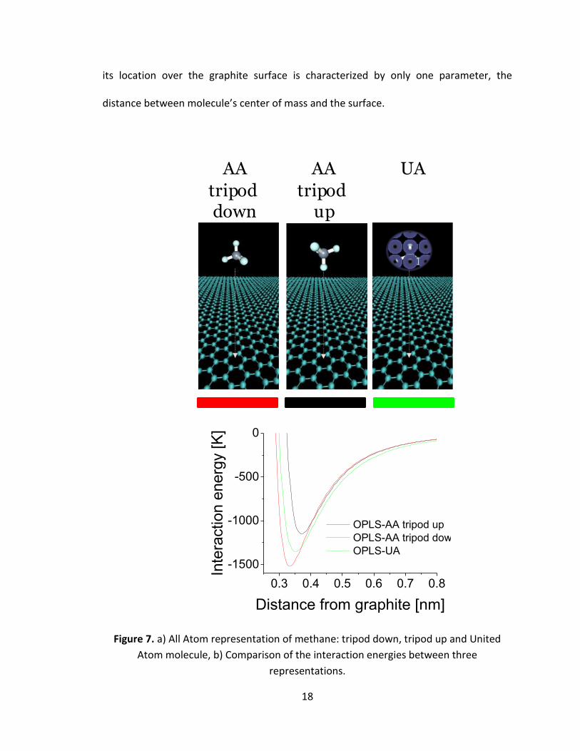
18

its location over the graphite surface is characterized by only one parameter, the

distance between molecule’s center of mass and the surface.

Figure 7. a) All Atom representation of methane: tripod down, tripod up and United

Atom molecule, b) Comparison of the interaction energies between three

representations.

AA

tripod down

AA

tripod up

UA

0.3 0.4 0.5 0.6 0.7 0.8

-1500

-1000

-500

0

OPLS-AA tripod up

OPLS-AA tripod down

OPLS-UA

Inte

raction e

nerg

y [K

]

Distance from graphite [nm]

19

Figure 7.b compares the methane-graphite interaction energies as a function of distance

of methane center of mass (central carbon atom in AA representation) from graphite, in

three configurations specified above. The Lennard-Jones 12-6 form of potential with

OPLS parameters was used, with a cutoff equal 1.5 nm. As it could be expected, the

strongest interaction with substrate is observed for the “tripod down” configuration

while in the case of the “tripod up” orientation the depth of the potential well is the

smallest. The energy minimum for UA model is placed in between the two extreme AA

situations.

Figure 8 compares the methane-graphite interaction energies calculated using OPLS

parameters with data available in the literature [3],[8],[2],[16]. Two configurations are

analyzed: “tripod down” (AA approach, Fig.8.a) and UA approximation (Fig.8.b). In both

cases the OPLS non-bonded parameters were implemented into Lennard-Jones 12-6

potential while the referenced solid-fluid parameters were inserted into the Steele 10-4-

4 potential. No significant difference between the literature data and our calculations

has been found. Strong overlapping of the plots is visible. This confirms that the OPLS-

AA and OPLS-UA parameters are consistent with force field parameters previously used

in numerical studies of methane adsorption and auto-organisation on graphite.

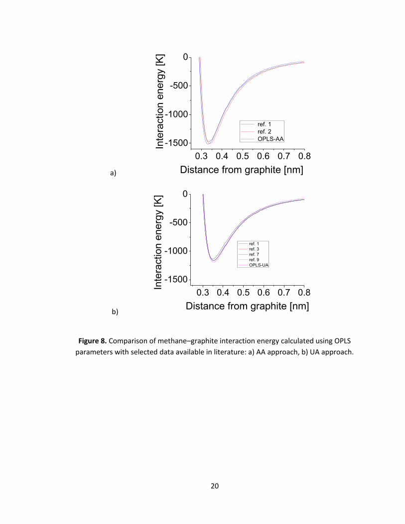
20

a)

b)

Figure 8. Comparison of methane–graphite interaction energy calculated using OPLS

parameters with selected data available in literature: a) AA approach, b) UA approach.

0.3 0.4 0.5 0.6 0.7 0.8

-1500

-1000

-500

0

Inte

raction e

nerg

y [K

]Distance from graphite [nm]

ref. 1

ref. 2

OPLS-AA

0.3 0.4 0.5 0.6 0.7 0.8

-1500

-1000

-500

0

Inte

raction e

nerg

y [K

]

Distance from graphite [nm]

ref. 1

ref. 3

ref. 7

ref. 9

OPLS-UA

21

We have also verified if the increase of the strength of methane-surface interaction with

increasing number of graphene layers forming the substrate is correctly reproduced

when OPLS parameters are used. Figure 9 shows the variation of methane-substrate

interaction in both UA and AA models when successive graphene layers are added.

There is no significant change in gas-substrate interaction energy when the substrate

contains a stack of three or more graphene sheets. This result is consistent with the

literature data showing that to simulate interactions of molecules with infinite (in

depth) graphite surface it is sufficient to model the graphite using only four layers of

graphene, at least if the cutoff of interactions is equal 1.5 nm.

22

a)

b)

Figure 9. Energy of methane interaction with 1, 2, 3, and 4 layers of graphene: a) UA

representation of methane, b) AA representation of methane (tripod down

configuration).

The simulations were carried out at 195 K (below the boiling point of methyl mercaptan,

279 K), at 298 K and 320 K. In order to verify the choice of force field parameters for

methyl mercaptan, test simulations of gas mixtures without graphene were first

conducted. Two molar fractions of thiols were chosen: 0.065 and 0.019 and systems

were equilibrated at the three chosen temperatures. At room temperature and 320 K

0.3 0.4 0.5 0.6 0.7 0.8

-1500

-1000

-500

0

Inte

raction e

nerg

y [K

]Distance from substrate [nm]

1 graphene layer

2 graphene layers

3 graphene layers

4 graphene layers

0.3 0.4 0.5 0.6 0.7 0.8

-1500

-1000

-500

0

Inte

raction e

nerg

y [K

]

Distance from substrate [nm]

1 graphene layer

2 graphene layers

3 graphene layers

4 graphene layers

23

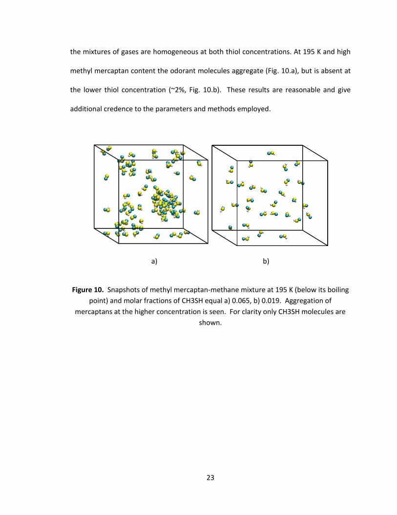
the mixtures of gases are homogeneous at both thiol concentrations. At 195 K and high

methyl mercaptan content the odorant molecules aggregate (Fig. 10.a), but is absent at

the lower thiol concentration (~2%, Fig. 10.b). These results are reasonable and give

additional credence to the parameters and methods employed.

a) b)

Figure 10. Snapshots of methyl mercaptan-methane mixture at 195 K (below its boiling

point) and molar fractions of CH3SH equal a) 0.065, b) 0.019. Aggregation of

mercaptans at the higher concentration is seen. For clarity only CH3SH molecules are

shown.

24

5. Results and discussion

5.1. Adsorption isotherms

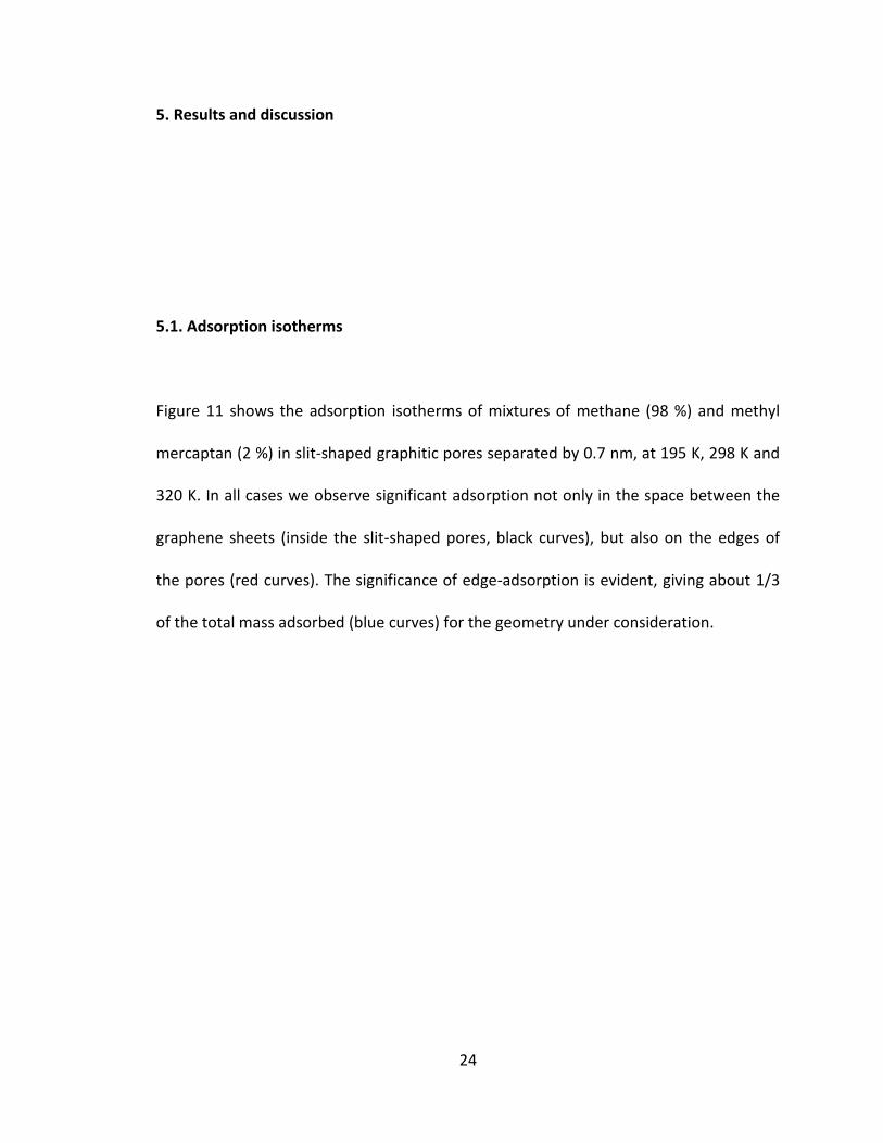
Figure 11 shows the adsorption isotherms of mixtures of methane (98 %) and methyl

mercaptan (2 %) in slit-shaped graphitic pores separated by 0.7 nm, at 195 K, 298 K and

320 K. In all cases we observe significant adsorption not only in the space between the

graphene sheets (inside the slit-shaped pores, black curves), but also on the edges of

the pores (red curves). The significance of edge-adsorption is evident, giving about 1/3

of the total mass adsorbed (blue curves) for the geometry under consideration.

25

a)

b)

c)

Figure 11. Adsorption isotherms of methane-mercaptan mixtures in 0.7 nm slits at a)

195 K, b) 298 K, c) 320K.

0 50 100 150 200 2500

50

100

150

200

250

300

Mass a

dso

rbed

[g/k

g C

]

in slit

on edges

total

p [bar]

0 50 100 150 200 2500

50

100

150

200

250

300

p [bar]

in slit

on edges

total

Mass a

dso

rbed

[g

/kg C

]

0 50 100 150 200 2500

50

100

150

200

250

300 in slit

on edges

total

p [bar]

Mass a

dso

rbed

[g

/kg C

]

26

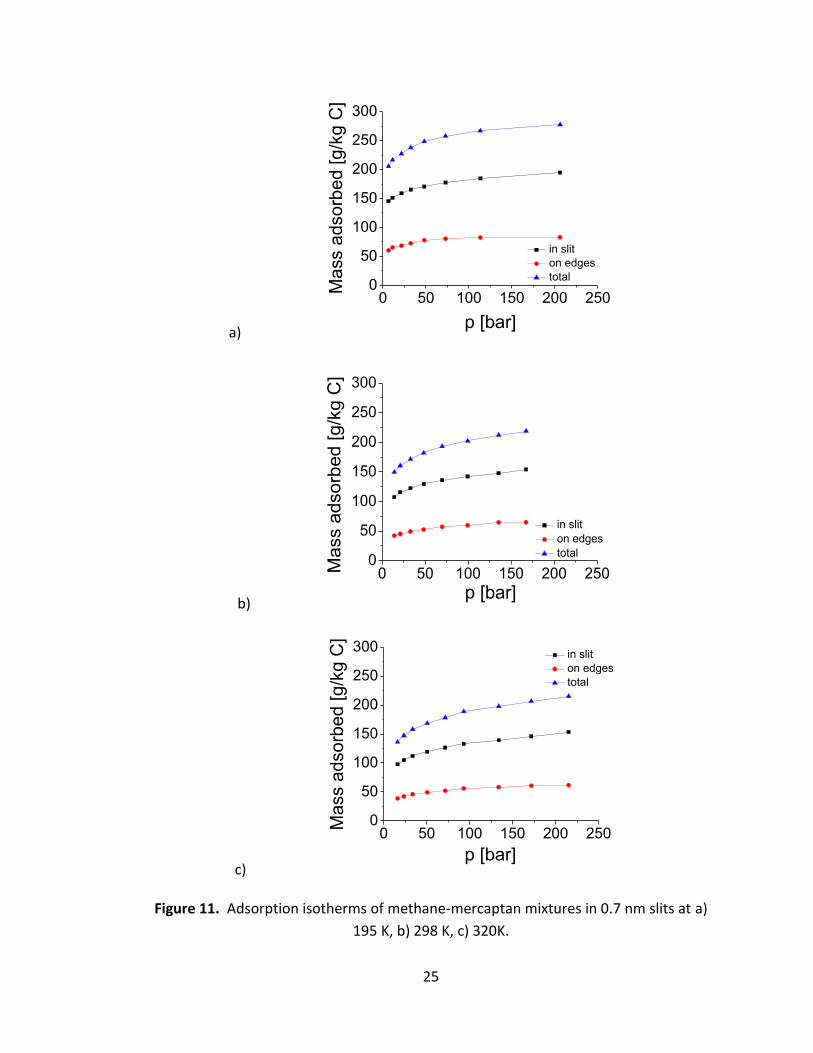
5.2. Adsorption energy: maximum value and fluctuations, mobility

In this section we present the analysis of plots of solid-fluid interaction energies as

functions of simulation frame number (1 frame = 100 fs) for methane- and methyl

mercaptan-graphene pairs separately at 195 K, 298 K and 320 K and various pressures.

For each system considered the strongest interaction energy is observed when gas

molecule is present between two graphitic sheets. The values of the strongest

interaction energies between methane-substrate and methyl mercaptan-substrate pairs

(averaged over the number of molecules) are presented in Table 4. Fluctuations of the

interaction energies are coupled with capability of both methane and mercaptan to

migrate between the gas phase and inner volume of the slit (Figs. 12 and 13).

Table 4. Energies of the strongest gas-substrate interactions.

196 K Methane Thiol 298 K Methane Thiol 320 K Methane Thiol

Pressure [bar]

Energy [K]

Energy [K]

Pressure [bar]

Energy [K]

Energy [K]

Pressure [bar]

Energy [K]

Energy [K]

6.5 -2,367 -4,056 21.0 -2,299 -4,101 16.2 -2,422 -4,147

21.5 -2,264 -4,052 48.8 -2,300 -4,096 33.7 -2,422 -4,147

48.1 -2,178 -3,993 99.5 -2,155 -4,071 71.5 -2,421 -4,147

113.0 -1,956 -3,939 167.0 -1,917 -3,982 215.0 -2,419 -4,146

27

Methyl mercaptan’s size (< 0.437 nm) could allow relatively free molecular movement in

a 0.7 nm pore. However the thiol group interacts more strongly with the graphene

(nearly 2 times stronger compared to methane-graphene), which could hinder its

motion and make the mercaptan adsorption irreversible. Given the small number of

mercaptans (and, in consequence, poor statistics for that component of the mixture), it

is difficult to obtain reliable adsorption/desorption isotherms for this component. We

thus focused on performing an energetic and dynamical analysis of the gas mixture.

Figures 12 and 13 show the time evolution of the interaction energy between

representative methane (Fig. 12) and methyl mercaptan (Fig. 13) molecules and

graphene slits at lowest and highest pressures achieved at each simulation temperature,

e.g., 6.5 bar and 206 bar at 195 K, 14.1 bar and 167 bar at 298 K, 16.2 bar and 215 bar at

320 K. In all cases methane molecules reveal dynamical behavior, and mobility increases

as the gas pressure increases due to saturation of the deepest adsorption sites.

The methyl mercaptan-substrate interaction energies also fluctuate significantly

throughout simulation time, even at temperature as low as 195 K (Fig. 13). Despite high

substrate-adsorbate interaction energy, mercaptan molecules remain mobile and

change their positions with respect to the slit. More significant energy fluctuations

appear at room and higher temperature. The mercaptan-graphene interaction energy

for some representative molecules was correlated with the changes in the center of

mass positions for the odorants in the z direction.

28

T = 195 K p = 6.5 bar

p = 206 bar

T = 298 K p = 14.1 bar

p = 167 bar

T = 320 K p = 16.2 bar

p = 215 bar

Figure 12. Graphene-methane interaction energy vs. time step for various

representative molecules. The variations in energy correspond to migrations between

slits and edges, and to the gas phase.

0 200 400 600 800 1000-2500

-2000

-1500

-1000

-500

0

En

erg

y [K

]

Time step

0 200 400 600 800 1000

-2000

-1500

-1000

-500

0

Energ

y [K

]

Time step

0 200 400 600 800 1000-2500

-2000

-1500

-1000

-500

0

Energ

y [K

]

Time step

0 200 400 600 800 1000-2500

-2000

-1500

-1000

-500

0

Energ

y [K

]

Time step

0 200 400 600 800 1000-2500

-2000

-1500

-1000

-500

0

En

erg

y [K

]

Time step

0 200 400 600 800 1000-2500

-2000

-1500

-1000

-500

0

En

erg

y [K

]

Time step

29

T = 195 K p = 6.5 bar

p = 206 bar

T = 298 K p = 14.1 bar

p = 167 bar

T = 320 K p = 16.2 bar

p = 215 bar

Figure 13. Graphene-mercaptan interaction energy vs. time step for various

representative molecules.

0 200 400 600 800 1000

-4000

-3000

-2000

-1000

0

Energ

y [K

]

Time step

0 200 400 600 800 1000

-4000

-3000

-2000

-1000

0

En

erg

y [K

]

Time step

0 200 400 600 800 1000

-4000

-3000

-2000

-1000

0

Energ

y [K

]

Time step

0 200 400 600 800 1000

-4000

-3000

-2000

-1000

0

En

erg

y [

K]

Time step

0 200 400 600 800 1000

-4000

-3000

-2000

-1000

0

Energ

y [K

]

Time step

0 200 400 600 800 1000

-4000

-3000

-2000

-1000

0

Time step

En

erg

y [

K]

30

5.3. Diffusion in adsorbed methane-methyl mercaptan mixtures

5.3.1. Graphene surface

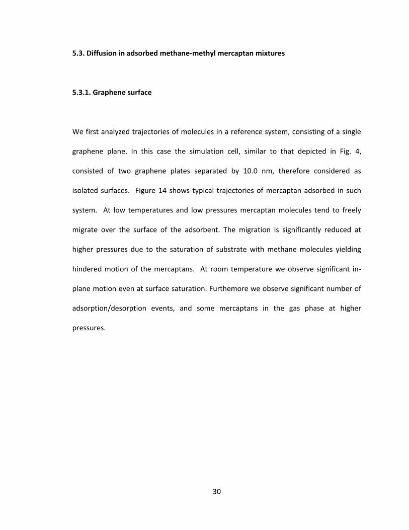
We first analyzed trajectories of molecules in a reference system, consisting of a single

graphene plane. In this case the simulation cell, similar to that depicted in Fig. 4,

consisted of two graphene plates separated by 10.0 nm, therefore considered as

isolated surfaces. Figure 14 shows typical trajectories of mercaptan adsorbed in such

system. At low temperatures and low pressures mercaptan molecules tend to freely

migrate over the surface of the adsorbent. The migration is significantly reduced at

higher pressures due to the saturation of substrate with methane molecules yielding

hindered motion of the mercaptans. At room temperature we observe significant in-

plane motion even at surface saturation. Furthemore we observe significant number of

adsorption/desorption events, and some mercaptans in the gas phase at higher

pressures.

31

a)

b)

c)

d)

Figure 14. Trajectories of a single methyl mercaptan on graphite surface. a) T = 195 K

and p = 1.2 bar, b) T = 195 K and p = 24.8 bar, c) T = 298 K and p = 3.6 bar, d) T = 298 K

and p = 69.7 bar.

z-d

ire

ctio

n [n

m]

0.0

10.0

0 0.5Time [ns]

10.00.0x-direction [nm]

0.0

10.0

y-d

ire

ctio

n [n

m]

x-direction [nm]0.5

Time [ns]

z-d

ire

ctio

n [n

m]

0.0

10.0

0 10.00.0

0.0

10.0

y-d

ire

ctio

n [n

m]

z-d

ire

ctio

n [n

m]

0.0

10.0

0 10.00.0x-direction [nm]

0.0

10.0

y-d

ire

ctio

n [n

m]

0.5Time [ns]

z-d

irection [nm

]

0.0

10.0

0 0.5Time [ns]

10.00.0x-direction [nm]

0.0

10.0

y-d

irection [nm

]

32

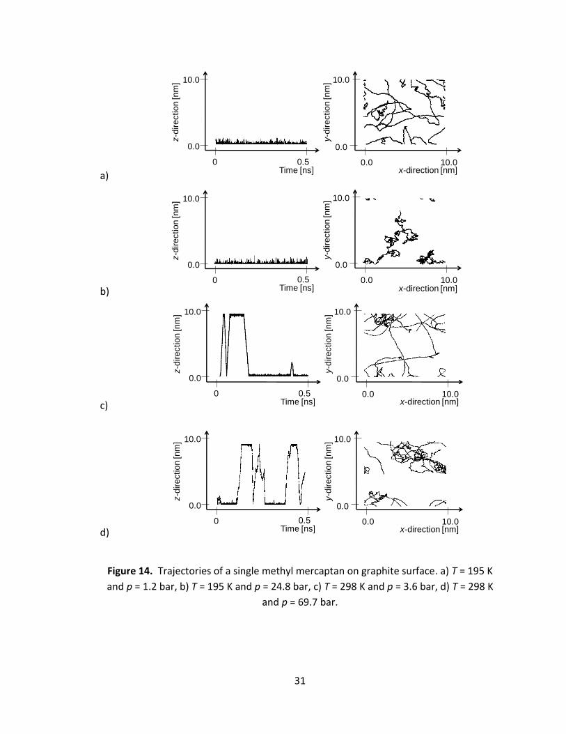
5.3.2. 0.7 nm slit-shaped pores

We now consider the mobility of methane and methyl mercaptan molecules adsorbed in

narrow, 0.7 nm wide pores. As mentioned earlier, such geometry provides the most

severe conditions (geometric and energetic) for adsorption and generates an extreme

adsorption scenario: highest adsorbed phase density and highest probability for

mercaptans to be trapped inside the pores. Figure 15 shows the trajectories of

mercaptan molecules in the simulation box, at moderate pressures and two

temperatures: 195 K and 298 K. At 195 K mercaptan molecules initially diffuse into the

pores but then their motion remains constrained to a limited fraction of the pore

volume. At 298 K mercaptan mobility is significantly higher; molecules rapidly move

inside the slit and are able to probe a wide area between the slits walls. In consequence

they can also desorb from one pore into the gas phase and then adsorb into another

one (Fig. 15, lower left panel), i.e., three-dimensional movement is possible.

33

a)

b)

Figure 15. Typical trajectories of single methyl mercaptan in 0.7 nm slit Left: side view,

right: top view. a) At T = 195 K, p = 21.5 bar an adsorption event and limited in-plane

diffusion. b) At T = 298 K, p = 167 bar the adsorption/desorption events and both in-

plane diffusion and out-of-plane movement.

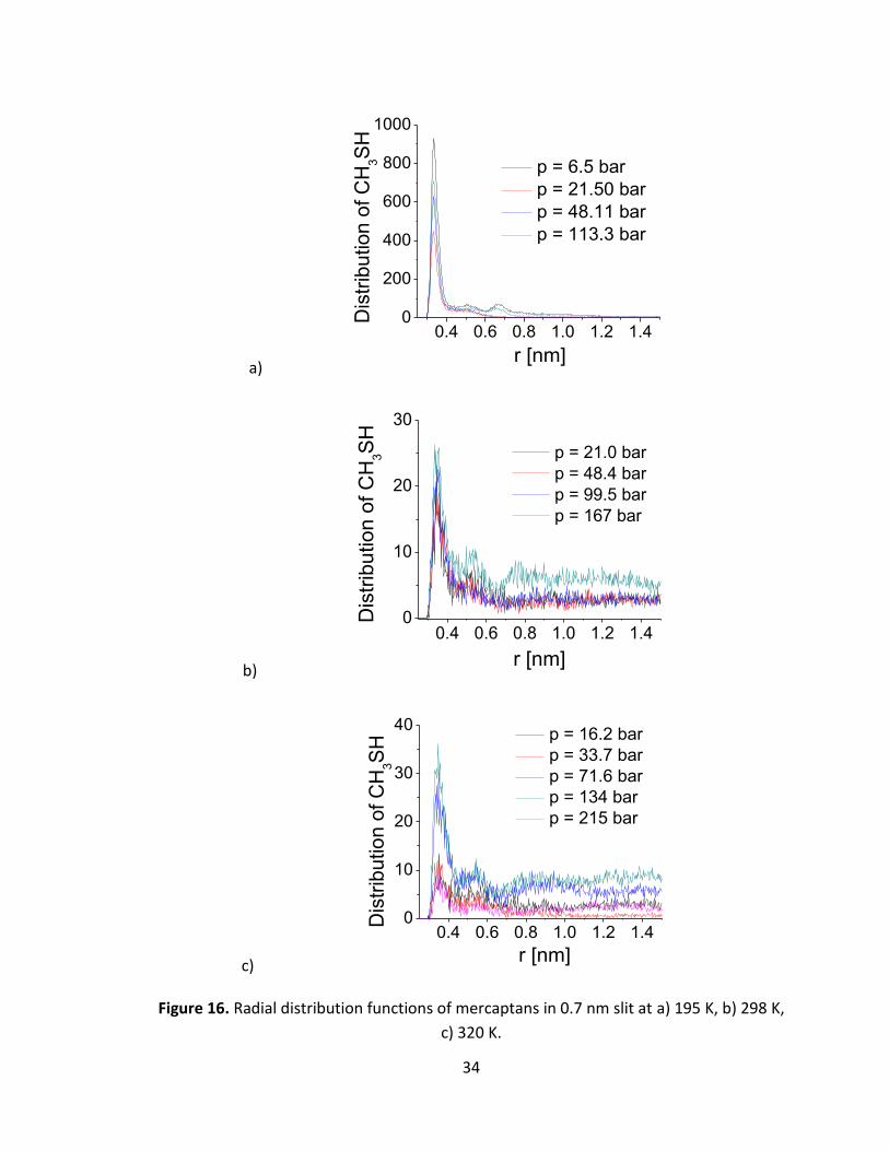
Figure 16 shows the radial distribution functions for mercaptan molecules in a 0.7 nm

slit pore at 195 K, 298 K and 320 K at various pressures. At 195 K the peaks of the

distribution function show tendency of the mercaptans to aggregate, contrary to what

happens in the 2 % methane-mercaptan mixtures in absence of the adsorbant (i.e., in

gas phase). At higher temperatures, the relatively less structured distribution function is

indicative of absence of aggregation.

! !

T=195K,p=21.5bar

! !

T=298K,p=167bar

34

a)

b)

c)

Figure 16. Radial distribution functions of mercaptans in 0.7 nm slit at a) 195 K, b) 298 K,

c) 320 K.

0.4 0.6 0.8 1.0 1.2 1.40

200

400

600

800

1000

r [nm]D

istr

ibu

tio

n o

f C

H3S

H

p = 6.5 bar

p = 21.50 bar

p = 48.11 bar

p = 113.3 bar

0.4 0.6 0.8 1.0 1.2 1.40

10

20

30

p = 21.0 bar

p = 48.4 bar

p = 99.5 bar

p = 167 bar

Dis

trib

utio

n o

f C

H3S

H

r [nm]

0.4 0.6 0.8 1.0 1.2 1.40

10

20

30

40

r [nm]

Dis

trib

utio

n o

f C

H3S

H

p = 16.2 bar

p = 33.7 bar

p = 71.6 bar

p = 134 bar

p = 215 bar

35

The dynamical behavior of methane and methyl mercaptan inside the graphitic slits was

further analyzed via the determination of the molecules’ mean square displacement

(MSD). We considered both MSDs in two dimensions (2D, the in-plane motion within a

slit), and three dimensions (3D, including migration between pores). In all cases

analyzed, MSDs grow linearly in time within the margin of error, indicating a normal

diffusion regime. Figure 17 shows in detail the 2D MSD’s for both methane and

mercaptans at various temperature and pressure values. Methane’s migration inside of

the slit volume decreases with increasing pressure. At 195 K mercaptan migration inside

the slit is the strongest at lowest gas pressure. With increasing temperature the mobility

of mercaptans depends on the amount of gas adsorbed. However, the differences

become smaller at and above the critical temperature. Finally, at 320 K no correlation is

seen between mercaptans’ mobility and the system pressure change.

Given the linear MSD vs. t observed in all cases, we calculated 2D and 3D self-diffusion

coefficients of methane and methyl mercaptan, according to the relation:

(14)

where d is the dimensionality of the problem (2 or 3) and t is the timestep. The resulting

diffusion constants are shown in Fig. 18.

36

a)

b)

c)

Figure 17. Two-dimensional mean square displacement as a function of simulation time

plots for methane and methyl mercaptan at a) 195K, b) 298 K and c) 320 K.

0.0 0.1 0.2 0.3 0.4 0.50

500

1000

1500

2000

2500

3000

Time [ns]M

SD

CH4

CH3SH

p = 6.5 bar

21.5 bar

48.1 bar

113 bar

0.0 0.1 0.2 0.3 0.4 0.50

2000

4000

6000

8000

10000

12000

Time [ns]

MS

D

CH4 CH3SH

p = 14.1 bar

33.0 bar

69.7 bar

135 bar

0.0 0.1 0.2 0.3 0.4 0.50

2000

4000

6000

8000

10000

12000

Time [ns]

MS

D

CH4 CH3SH

p = 16.2 bar

33.6 bar

74.1 bar

134 bar

215 bar

37

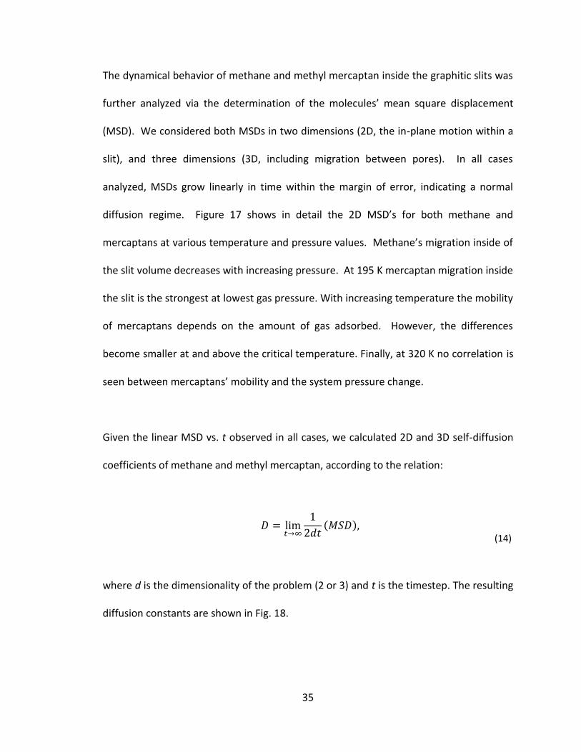
a)

b)

c)

Figure 18. Diffusion coefficients vs. pressure at a) 195 K, b) 298 K and c) 320 K.

0 50 100 150 200 2500

1

2

3

4

5

6

D [10

8 m

2/s

]

p [bar]

CH4 2D

CH4 3D

CH3SH 2D

CH3SH 3D

0 50 100 150 200 2500

5

10

15

20

25

CH4 2D

CH4 3D

CH3SH 2D

CH3SH 3D

D [10

8 m

2/s

]

p [bar]

0 50 100 150 200 2500

5

10

15

20

25

CH4 2D

CH4 3D

CH3SH 2D

CH3SH 3D

p [bar]

D [10

8 m

2/s

]

38

5.4. Required enhancement of mercaptan concentration in natural gas

In order to detect natural gas leaks, the concentration of mercaptans in the gas phase

should be above ca. 200 ppb (see discussion in Section 1). Since mercaptans bind to

graphite more strongly than methane (Table 4), it is necessary to increase their

concentration in the adsorbed phase so that any amount desorbed contains at least the

required concentration. Here we present a qualitative assessment of mercaptan

concentrations for detectability; therefore, because of important safety considerations,

experiments will inevitably have to yield quantitative detectability results. To evaluate

the required mercaptan concentration we have assumed that:

(i) Interaction between adsorbed molecules will be neglected (a decent, though

not quantitatively correct, assumption for supercritical adsorption);

(ii) Quantum mechanical effects are small (a very reasonable assumption for

relatively heavy molecules at the temperatures considered. The thermal

wavelength for methane at room temperature

much smaller than any other distance considered in the present study);

(iv) The molar volume of the adsorbed phase is much smaller than that of the gas

phase (reasonable except at pressures near saturation); and

(v) The ideal gas law applies for the gas phase.

39

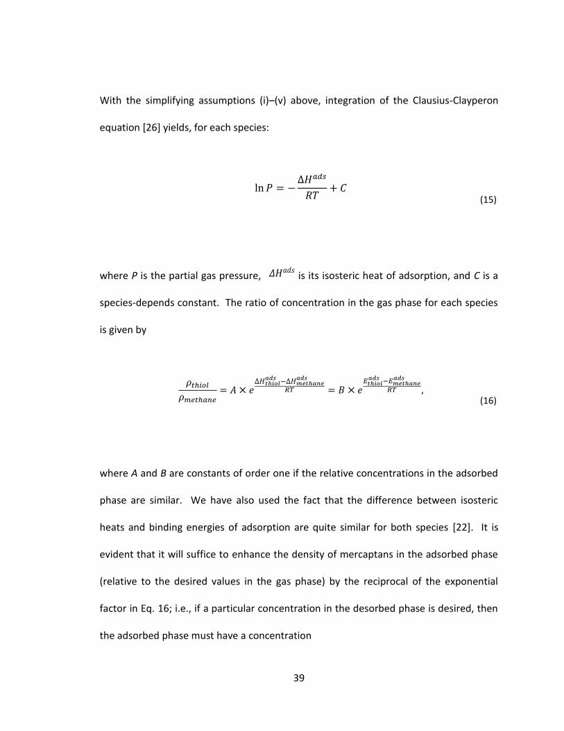
With the simplifying assumptions (i)–(v) above, integration of the Clausius-Clayperon

equation [26] yields, for each species:

(15)

where P is the partial gas pressure, is its isosteric heat of adsorption, and C is a

species-depends constant. The ratio of concentration in the gas phase for each species

is given by

(16)

where A and B are constants of order one if the relative concentrations in the adsorbed

phase are similar. We have also used the fact that the difference between isosteric

heats and binding energies of adsorption are quite similar for both species [22]. It is

evident that it will suffice to enhance the density of mercaptans in the adsorbed phase

(relative to the desired values in the gas phase) by the reciprocal of the exponential

factor in Eq. 16; i.e., if a particular concentration in the desorbed phase is desired, then

the adsorbed phase must have a concentration

𝛥 𝑎 𝑠

40

𝑎

𝑎

𝑎 𝑠 𝑎

𝑎 𝑠

(17)

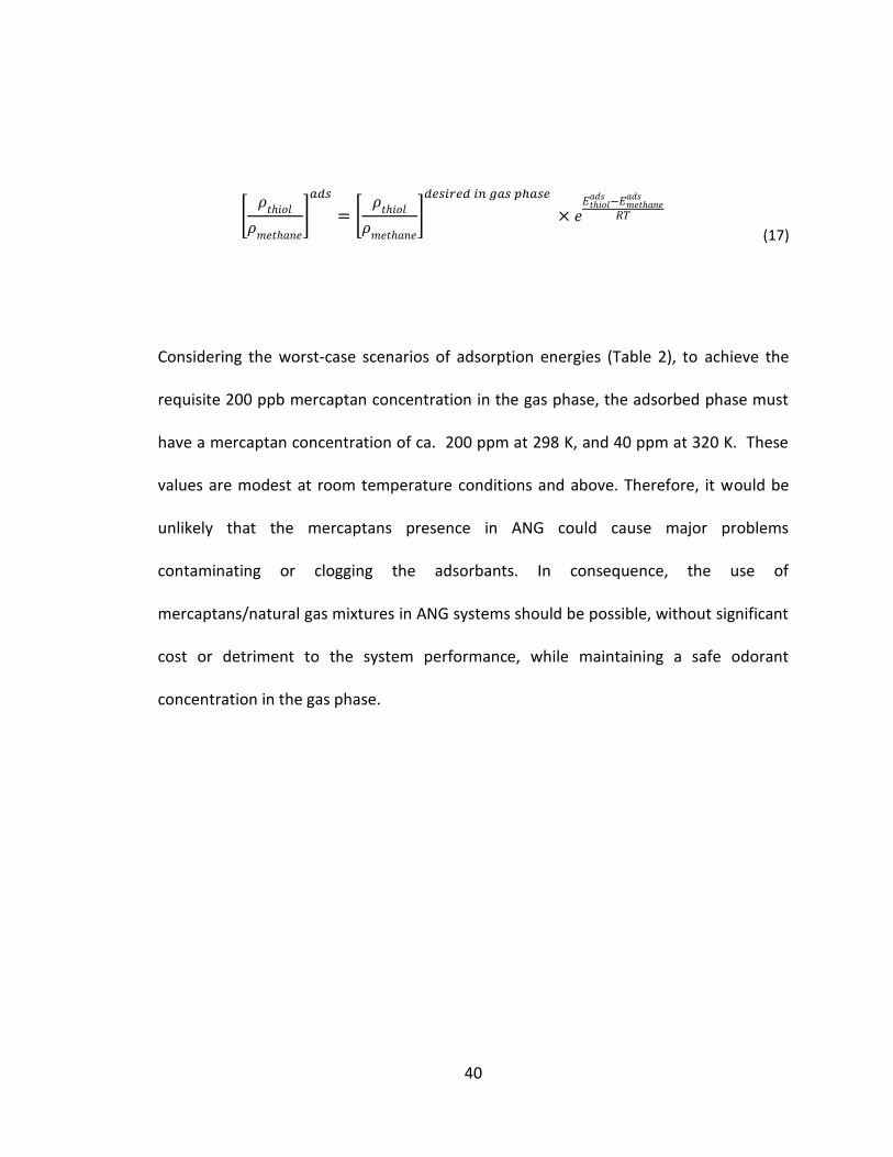
Considering the worst-case scenarios of adsorption energies (Table 2), to achieve the

requisite 200 ppb mercaptan concentration in the gas phase, the adsorbed phase must

have a mercaptan concentration of ca. 200 ppm at 298 K, and 40 ppm at 320 K. These

values are modest at room temperature conditions and above. Therefore, it would be

unlikely that the mercaptans presence in ANG could cause major problems

contaminating or clogging the adsorbants. In consequence, the use of

mercaptans/natural gas mixtures in ANG systems should be possible, without significant

cost or detriment to the system performance, while maintaining a safe odorant

concentration in the gas phase.

41

6. Summary and Conclusions

The goal of this study was to analyze the feasibility of incorporating odorant molecules

in ANG systems. We focused on adsorption of gas mixtures in semi-finite, 0.7 nm wide

pores in a wide range of pressures and temperatures of 195 K, 298 K and 320 K. The

geometry of the pore was chosen to model the extreme situation, with strongest

adsorption potentials (due to the superposition of the van der Waals contribitions from

both pore walls) and molecular motion that is strongly hindered (steric constrains in

narrow pores). We believe that this geometry represents the most irreversible

conditions for the adsorption, in particular of mercaptans, due to their strength of

binding to the substrate.

Our analysis shows that even in constrained geometries the adsorption of methane and

odorant molecules remains reversible. Methyl mercaptan is able to migrate within the

pore volume, desorb and/or migrate between pores. Even though mercaptans bind to

the adsorbent’s surface more strongly than methane, only a relatively modest increase

of mercaptan concentration in the adsorbed phase is necessary to keep its

concentration in the gas phase above human detection threshold. The estimated

concentration levels in the adsorbed phase are in the parts per million (vs. parts per

billion in the gas phase). It appears to be unlikely that at suggested odorants’

concentrations pore clogging would be significant. From this perspective, a safe ANG

42

tank should be able to operate continuously for numerous charge-discharge

(adsorption-desorption) cycles before any additional processing is needed (such as

moderate heating of the ANG tank while connected to a vacuum pump). Our studies

show that odorant molecules can be used in ANG systems for enhanced security without

major increase in cost and without adsorbent poisoning.

43

References

[1] United States Federal Register 49 CFR 192.625(a), Canadian Standards Organization Z662-99 Sect. 4.17.1

[2] Albesa A G, Llanos J L and Vicente J 2009 Comparative Study of Methane Adsorption on Graphite Langmuir 24 3836-40

[3] Ayappa K G and Ghatak C 2002 The structure of frozen phases in slit nanopores: A grand canonical Monte Carlo study J. Chem. Phys. 117 5373-83

[4] Bashkova S, Bagreev A and Bandosz T J 2002 Effect of Surface Characteristics on Adsorption of Methyl Mercaptan on Activated Carbons Ind. Eng. Chem. Res. 41 4346-52

[5] Bhatia S K and Myers A L 2006 Optimum Conditions for Adsorptive Storage Langmuir 22 1688-700

[6] Dai X D, Liu X M, Qian L, Qiao K and Yan Z F 2008 Pilot Preparation of Activated Carbon for Natural Gas Storage Energy Fuels 22 3420-3

[7] Davies G M and Seaton N A 1998 The effect of the choice of pore model on the characterization of the internal structure of microporous carbons using pore size distribution Carbon 36 1473-90

[8] Do D D and Do H D 2005 Evaluation of 1-Site and 5-Site Models of Methane on Its Adsorption on Graphite and in Graphitic Slit Pores J. Phys. Chem. B 109 19288-95

[9] El-Sheikha S M, Barakat K and Salem N M 2006 Phase transitions of methane using molecular dynamics simulations J. Chem. Phys. 124

[10] Gusev V Y and O’Brien J A 1997 A Self-Consistent Method for Characterization of Activated Carbons Using Supercritical Adsorption and Grand Canonical Monte Carlo Simulations Langmuir 13 2815-21

[11] He Y and Seaton N A 2005 Monte Carlo Simulation and Pore-Size Distribution Analysis of the Isosteric Heat of Adsorption of Methane in Activated Carbon Langmuir 21 8297–301

[12] Jorgensen W L 1998 OPLS Force Fields. vol 3 (New York: Wiley) [13] MacKerell J, A.D., Brooks B, Brooks I, C.B. , Nilsson L, Roux B, Won Y and Karplus

M 1998 CHARMM: The Energy Function and Its Parametrization with an Overview of the Program vol 1 (Chichester: Wiley & sons)

[14] Martin M G and Siepmann J I 1998 Transferable Potentials for Phase Equilibria. 1. United-Atom Description of n-Alkanes J. Phys. Chem. B 102 2469-577

[15] Matrangaa K R, Myers A L and Glandt E D 1992 Storage of natural gas by adsorption on activated carbon Chemical Engineering Science 47 1569-79

[16] Nguyen T X, Bhatia S K and Nicholson D 2002 Close packed transitions in slit-shaped pores: Density functional theory study of methane adsorption capacity in carbon J. Chem. Phys. 11 10827-36

[17] Nicholson D 1998 Simulation studies of methane transport in model graphite micropores Carbon 36 1511-23

44

[18] Pfeifer P, Burress J W, Wood M B, Lapilli C M, Barker S A, Pobst J S, Cepel R J, Wexler C, Shah P S, Gordon M J, Suppes G J, Buckley S P, Radke D J, Ilavsky J, Dillon A C, Parilla P A, Benham M, Roth M W and Savage N 2008 High-Surface-Area Biocarbons for Reversible On-Board Storage of Natural Gas and Hydrogen Mater. Res. Soc. Symp. Proc. 1041 1041-R02-02

[19] Phillips J C, Braun R, Wang W, Gumbart J, Tajkhorshid E, Villa E, Chipot C, Skeel R D, Kale L and Schulten K 2005 Scalable Molecular Dynamics with NAMD J. Comput. Chem. 26 1781-802

[20] Ravikovitch P I, Vishnyakov A, Russo R and Neimark A V 2000 Unified Approach to Pore Size Characterization of Microporous Carbonaceous Materials from N2, Ar, and CO2 Adsorption Isotherms Langmuir 16 2311-20

[21] Schlick T 2006 Molecular modeling and simulation: An interdisciplinary guide vol 21 (New York: Springer Science+Business Media, LLC)

[22] Sircar S, Mohr R, Ristic C and Rao M B 1999 Isosteric Heat of Adsorption: Theory and Experiment J. Phys. Chem. B 103

[23] Sweatman M B and Quirke N 2001 Characterization of Porous Materials by Gas Adsorption at Ambient Temperatures and High Pressure J. Phys. Chem. B 105 1403-11

[24] Sweatman M B and Quirke N 2005 Gas Adsorption in Active Carbons and the Slit-Pore Model 1: Pure Gas Adsorption J. Phys. Chem. B 109 10381-8

[25] Tafipolsky M, Amirjalayer S and Schmid R 2009 Atomistic theoretical models for nanoporous hybrid materials Microporous and Mesoporous Materials 124 110–6

[26] Wark and Kenneth (1988) [1966] Generalized Thermodynamic Relationships. (New York, NY: McGraw-Hill, Inc. )