Finance and Economics Discussion SeriesDivisions of Research & Statistics and Monetary Affairs

Federal Reserve Board, Washington, D.C.

The Risky Steady State and the Interest Rate Lower Bound

Timothy S. Hills, Taisuke Nakata, and Sebastian Schmidt

2016-009

Please cite this paper as:Hills, Timothy S., Taisuke Nakata, and Sebastian Schmidt (2016). “The Risky SteadyState and the Interest Rate Lower Bound,” Finance and Economics Discussion Se-ries 2016-009. Washington: Board of Governors of the Federal Reserve System,http://dx.doi.org/10.17016/FEDS.2016.009.

NOTE: Staff working papers in the Finance and Economics Discussion Series (FEDS) are preliminarymaterials circulated to stimulate discussion and critical comment. The analysis and conclusions set forthare those of the authors and do not indicate concurrence by other members of the research staff or theBoard of Governors. References in publications to the Finance and Economics Discussion Series (other thanacknowledgement) should be cleared with the author(s) to protect the tentative character of these papers.

The Risky Steady State and the Interest Rate Lower Bound∗

Timothy Hills†

New York University

Taisuke Nakata‡

Federal Reserve Board

Sebastian Schmidt§

European Central Bank

This Draft: January 2016

Abstract

Even when the policy rate is currently not constrained by its effective lower bound (ELB), the

possibility that the policy rate will become constrained in the future lowers today’s inflation

by creating tail risk in future inflation and thus reducing expected inflation. In an empirically

rich model calibrated to match key features of the U.S. economy, we find that the tail risk

induced by the ELB causes inflation to undershoot the target rate of 2 percent by as much

as 45 basis points at the economy’s risky steady state. Our model suggests that achieving

the inflation target may be more difficult now than before the Great Recession, if the recent

ELB experience has led households and firms to revise up their estimate of the ELB frequency.

JEL: E32, E52

Keywords: Deflationary Bias, Disinflation, Inflation Targeting, Risky Steady State, Tail Risk,

Zero Lower Bound.

∗We would like to thank Lena Boneva, Oliver de Groot, Michael Kiley, Jean-Philippe LaForte, John Robertsand seminar participants at the University of Tokyo for useful comments. Paul Yoo provided excellent researchassistance. The views expressed in this paper, and all errors and omissions, should be regarded as those solelyof the authors, and are not necessarily those of the Federal Reserve Board of Governors, the Federal ReserveSystem, or the European Central Bank.†Stern School of Business, New York University, 44 West 4th Street New York, NY 10012; Email:

hills.timoteo@gmail.com‡Division of Research and Statistics, Federal Reserve Board, 20th Street and Constitution Avenue N.W.

Washington, D.C. 20551; Email: taisuke.nakata@frb.gov§European Central Bank, Monetary Policy Research Division, 60640 Frankfurt, Germany; Email: sebas-

tian.schmidt@ecb.int.

1

1 Introduction

This paper characterizes the risky steady state in an empirically rich sticky-price model

with occasionally binding effective lower bound (ELB) constraints on nominal interest rates.

The risky steady state is the “point where agents choose to stay at a given date if they

expect future risk and if the realization of shocks is 0 at this date” (Coeurdacier, Rey, and

Winant (2011)). The risky steady state is an important object in dynamic macroeconomic

models: This is the point around which the economy fluctuates, the point where the economy

eventually converges to when all headwinds and tailwinds dissipate.

We first use a stylized New Keynesian model to illustrate how, and why, the risky steady

state differs from the deterministic steady state. We show that inflation and the policy rate

are lower, and output is higher, at the risky steady state than at the deterministic steady

state. This result obtains because the lower bound constraint on interest rates makes the

distribution of firm’s marginal costs of production asymmetric; the decline in marginal costs

caused by a large negative shock is larger than the increase caused by a positive shock of

the same magnitude. As a result, the ELB constraint reduces expected marginal costs for

forward-looking firms, leading them to lower their prices even when the policy rate is not

currently constrained. Reflecting the lower inflation rate at the risky steady state, the policy

rate is lower at the risky steady state than at the deterministic steady state. In equilibrium,

the expected real rate is lower at the risky steady than at the deterministic steady state, and

the output gap is positive as a result. These qualitative results are consistent with those in

Adam and Billi (2007) and Nakov (2008) on how the ELB risk affects the economy near the

ELB constraint under optimal discretionary policy.

We then turn to the main exercise of our paper, which is to explore the quantitative im-

portance of the wedge between the risky and deterministic steady states in an empirically rich

DSGE model calibrated to match key features of the U.S. economy. We find that the wedge

between the deterministic and risky steady states is non-trivial in our calibrated empirical

model. Inflation is about 25 basis points lower than the target inflation of 2 percent at the

risky steady state, with 18 basis points attributable to the ELB constraint as opposed to other

nonlinearities of the model. The policy rate and the output gap are 50 basis points lower and

0.3 percentage points higher, respectively, at the risky steady state than at the deterministic

steady state. The magnitude of the wedge depends importantly on the frequency of hitting

the ELB, which in turn depends importantly on the level of the long-run equilibrium policy

rate. If the policy rate at the deterministic steady state is 40 basis points lower than our

baseline of 3.75 percent, then the deflationary bias would increase to more than 50 basis

points, with the ELB risk contributing 45 basis points to the overall deflationary bias.

The observation that inflation falls below the inflation target in the policy rule at the

risky steady state is different from the well-known fact that the average inflation falls below

the target rate in the model with the ELB constraint. The decline in inflation arising from

2

a contractionary shock can be exacerbated when the policy rate is at the ELB, while the

rise in inflation arising from an expansionary shock is tempered by a corresponding increase

in the policy rate. As a result, the distribution of inflation is negatively skewed and the

average inflation falls below the median. This fact is intuitive and has been well known in

the profession for a long time (Coenen, Orphanides, and Wieland (2004) and Reifschneider

and Williams (2000)). The risky steady state inflation is different from the average inflation;

it is the rate of inflation that would prevail at the economy’s steady state when agents are

aware of risks. It is worth mentioning that the average inflation falls below the target even

in perfect-foresight models or backward-looking models where the inflation rate eventually

converges to its target. On the other hand, for the risky steady state inflation to fall below

the inflation target, it is crucial that price-setters are forward-looking and take tail risk in

future marginal costs into account in their pricing decisions.

Our result that the ELB constraint has enduring effects on the economy even after liftoff

provides a cautionary tale for policymakers aiming to overcome the problem of persistently

low inflation. In particular, according to our model, inflation at the risky steady state is

tightly linked to how frequently the policy rate will be constrained by the ELB in the future.

Thus, our model suggests that achieving the inflation target may be more difficult now than

before the Great Recession, if the recent lower bound experience, together with the recent

downward assessment of the long-run growth rate of the economy and long-run equilibrium

policy rate, have made the private sector to increase its assessment of the likelihood of hitting

the ELB in the future.

The question of how the possibility of returning to the ELB affects the economy has

remained largely unexplored. The majority of the literature adopts the assumption that the

economy will eventually return to an absorbing state where the policy rate is permanently

away from the ELB constraint, and analyzes the dynamics of the economy, and the effects

of various policies, when the policy rate is at the ELB (Eggertsson and Woodford (2003),

Christiano, Eichenbaum, and Rebelo (2011)). While an increasing number of studies have

recently departed from the assumption of an absorbing state, the focus of these studies is

mostly on how differently the economy behaves at the ELB versus away from the ELB, instead

of how the ELB risk affects the economy away from the ELB.1 With the federal funds rate

finally raised from the ELB constraint after staying there for seven years, and with the pace of

the policy tightening expected to be gradual, the question of how the possibility of returning

to the ELB affects the economy is as relevant as ever.2

Our paper builds on the work by Adam and Billi (2007) and Nakov (2008) who first

1For example, Gavin, Keen, Richter, and Throckmorton (2015) and Keen, Richter, and Throckmorton(2015) ask how differently technology and anticipated monetary policy shocks affect the economy when thepolicy rate is constrained than when it is not, respectively. Schmidt (2013) and Nakata (2013a) ask howdifferently the government should conduct fiscal policy when the policy rate is at the ELB than when it is not.

2According to a special question in the Survey of Primary Dealers on December 2015, a median respondentattached 20 percent probability to the event that the federal funds rate returns to the ELB within two yearsafter liftoff.

3

observed that the possibility of returning to the ELB has consequences for the economy even

when the policy rate is currently away from the ELB. Our work differs from these papers in

two substantive ways. First, while they pointed out the anticipation effect of returning to the

ELB on the economy when the policy rate is near the ELB and the economy is away from the

steady state, our work shows that the possibility of returning to the ELB has consequences

for the economy even when the policy rate is well above the ELB and the economy is at the

steady state. Second, while they studied the effects of the ELB risk in a highly stylized model,

we quantify the magnitude of the effects of the ELB risk in an empirically rich, calibrated

model.

Our work complements a body of work that explores the so-called deflationary steady

state in sticky price models. A seminal work of Benhabib, Schmitt-Grohe, and Uribe (2001)

shows the existence of a deflationary steady state with the policy rate stuck at the lower

bound and inflation below target in a standard sticky-price model with a Taylor rule. Some

have recently studied deflationary steady states with zero nominal interest rates in other

interesting models with a nominal friction and a Taylor rule (Benigno and Fornaro (2015);

Eggertsson and Mehrotra (2014); Schmitt-Grohe and Uribe (2013)). Bullard (2010) argues

that these deflationary steady states are relevant in understanding the Japanese economy over

the last two decades as well as what may happen in other advanced economies. The steady

state we focus on is similar to the deflationary steady state in that both entail below-target

inflation. However, unlike in the deflationary steady state, the nominal interest rate is above

the ELB in the risky steady state.

Finally, this paper is related to recent papers that have emphasized the importance of

the effect of risk on steady states in various nonlinear dynamic models. de Groot (2014)

and Gertler, Kiyotaki, and Queralto (2012) discuss how the degree of risk affects the balance

sheet conditions of financial intermediaries at the steady state. Coeurdacier, Rey, and Winant

(2011), Devereux and Sutherland (2011) and Tille and van Wincoop (2010) study optimal

portfolio choices at the risky steady state in open-economy models. Our work is similar

to theirs in analyzing the effect of risk on the steady state. However, while the wedge

between the deterministic and risky steady states is driven by the nonlinearity of smooth

differentiable functions in their models, the wedge is driven by an inequality constraint in our

model. Reflecting the difference in the types of nonlinearity involved, the solution methods

employed are different. While these authors solve their models by using local approximation

methods that take advantage of differentiability of policy functions, we use a global method

to solve the model.3

The rest of the paper is organized as follows. After a brief review of the concept of

the risky steady state in section 2, Section 3 analyzes the risky steady state in a stylized

New Keynesian economy. Section 4 quantifies the wedge between the deterministic and risky

3See de Groot (2013) and Meyer-Gohde (2015) for recent progress in computing the risky steady state innonlinear differentiable economies.

4

steady states in an empirically rich DSGE model. After putting our analysis in the context

of the current policy debate in Section 5, section 6 concludes.

2 The Risky Steady State: Definition

The risky steady state is defined generically as follows.

Let Γt and St denote vectors of endogenous and exogenous variables, respectively, in the

model under investigation. Let f(·, ·) denote a vector of policy functions mapping the values

of endogenous variables in the previous period and today’s realizations of exogenous variables

into the values of endogenous variables today.4 That is,

Γt = f(Γt−1, St) (1)

The risky steady state of the economy, ΓRSS , is given by a vector satisfying the following

condition.

ΓRSS = f(ΓRSS , SSS) (2)

where SSS denote the steady state of St.5 That is, the risky steady state is where the economy

will eventually converge as the exogenous variables settle at their steady state. In this risky

steady state, the agents are aware that shocks to the exogenous variables can occur, but the

current realizations of those shocks are zero. On the other hand, the deterministic steady

state of the economy, ΓDSS , is defined as follows:

ΓDSS = fPF (ΓDSS , SSS) (3)

where fPF (·, ·) denotes the vector of policy functions obtained under the perfect-foresight

assumption.

3 The Risky Steady State in a Stylized Model with the ELB

3.1 Model

We start by characterizing the risky steady state in a stylized New Keynesian model.

Since the model is standard, we only present its equilibrium conditions here. The details of

the model are described in the Appendix A.

C−χct = βδtRtEtC−χct+1 Π−1

t+1 (4)

4Note that the policy function does not need to depend on the entire set of the endogenous variables inthe prior period. It may not depend on any endogenous variables in the prior period at all, as in the stylizedmodel presented in the next section.

5There is no distinction between deterministic and risky steady states for St because St is exogenous.

5

wt = Nχnt Cχct (5)

YtCχct

[ϕ

(Πt

Π− 1

)Πt

Π− (1− θ)− θwt

]= βδtEt

Yt+1

Cχct+1

ϕ

(Πt+1

Π− 1

)Πt+1

Π(6)

Yt = Ct +ϕ

2

[Πt

Π− 1

]2

Yt (7)

Yt = Nt (8)

Rt = max

[RELB,

Π

β

(Πt

Π

)φπ (YtY

)φy](9)

(δt − 1) = ρδ(δt−1 − 1) + εδt (10)

C, N , Y , w, Π, and R are consumption, labor supply, output, real wage, inflation, and

the policy rate, respectively. δ is an exogenous shock to the household’s discount rate, and

follows an AR(1) process with mean one, as shown in equation 10. Equation 4 is the consump-

tion Euler equation, Equation 5 is the intratemporal optimality condition of the household,

Equation 6 is the optimality condition of the intermediate good producing firms relating to-

day’s inflation to real marginal cost today and expected inflation tomorrow (forward-looking

Phillips Curve), Equation 7 is the aggregate resource constraint capturing the resource cost

of price adjustment, and Equation 8 is the aggregate production function. Equation 9 is the

interest-rate feedback rule where Π and Y are the central bank’s objectives for inflation and

output.

A recursive equilibrium of this stylized economy is given by a set of policy functions for

{C(·), N(·), Y (·), w(·), Π(·), R(·)} satisfying the equilibrium conditions described above.

The model is solved with a global solution method described in detail in the Appendix C.

Table 1 lists the parameter values used for this exercise.

Table 1: Parameter Values for the Stylized Model

Parameter Description Parameter Value

β Discount rate 11+0.004365

χc Inverse intertemporal elasticity of substitution for Ct 1.0χn Inverse labor supply elasticity 1θ Elasticity of substitution among intermediate goods 11ϕ Price adjustment cost 200400(Π− 1) (Annualized) target rate of inflation 2.0φπ Coefficient on inflation in the Taylor rule 1.5φy Coefficient on the output gap in the Taylor rule 0RELB The effective lower bound 1ρ AR(1) coefficient for the discount factor shock 0.8σε The standard deviation of shocks to the discount factor 0.24

100*The implied prob. that the policy rate is at the lower bound 10%

6

Figure 1: Policy Functions from the Stylized Model

1 1.002 1.004 1.006 1.0080

0.5

1

1.5

2

2.5

3

3.5

4

An

nu

aliz

ed

%

δ

Nominal Interest Rate

Deterministic St.St.

Risky St.St.

1 1.002 1.004 1.006 1.008−4

−3

−2

−1

0

1

2

An

nu

aliz

ed

%

δ

Inflation

Deterministic St.St.

Risky St.St.

1 1.002 1.004 1.006 1.008−2.5

−2

−1.5

−1

−0.5

0

0.5

% D

evia

tio

n f

rom

the

De

t. S

tea

dy S

tate

δ

Output

Deterministic St.St.

Risky St.St.

1 1.002 1.004 1.006 1.008−6

−5

−4

−3

−2

−1

0

1

An

nu

aliz

ed

%

δ

Real Wage

1 1.002 1.004 1.006 1.0080

0.5

1

1.5

2

2.5

3

An

nu

aliz

ed

%

δ

Exp. Real Rate

With uncertainty

Without uncertainty

Deterministic St.St.

Risky St.St.

*The dashed black lines (“Without uncertainty” case) show policy functions obtained under the perfect-foresight as-sumption (i.e., σε = 0).

3.2 Dynamics and the risky steady state

Before analyzing the risky steady state of the model, it is useful first to look at the

dynamics of the model. Solid black lines in Figure 1 show the policy functions for the policy

rate, inflation, output, and the expected real interest rate. Dashed black lines show the

policy function of the model obtained under the assumption of perfect foresight. Under the

perfect-foresight case, the agents in the model attach zero probability to the event that the

policy rate will return to the ELB when the policy rate is currently away from the ELB.

Under both versions of the model, an increase in the discount rate makes households want to

save more for tomorrow and spend less today. Thus, as δ increases, output, inflation, and the

policy rate decline. When δ is large and the policy rate is at the ELB, an additional increase

in the discount rate leads to larger declines in inflation and output than when δ is small and

the policy rate is not at the ELB, as the adverse effects of the increase in δ are not countered

7

by a corresponding reduction in the policy rate.

When the policy rate is at the ELB, the presence of uncertainty reduces inflation and

output. This is captured by the fact that the solid lines are below the dashed lines for

inflation and output in the figure. The non-neutrality of uncertainty is driven by the ELB

constraint. If the economy is buffeted by a sufficiently large expansionary shock, then the

policy rate will adjust to offset some of the resulting increase in real wages. If the economy is

hit by a contractionary shock, regardless of the size of the shock, the policy rate will stay at

the ELB and the resulting decline in real wages will not be tempered. Due to this asymmetry,

an increase in uncertainty reduces the expected real wage, which in turn reduces inflation as

price-setters are forward-looking and thus inflation today depends on the expected real wage.

With the policy rate constrained at the ELB, a reduction in inflation leads to an increase in

the expected real rate, pushing down consumption and output today. These adverse effects

of uncertainty at the ELB are studied in detail in Nakata (2013b).

When the policy rate is away from the ELB, the presence of uncertainty reduces inflation

and the policy rate, but increases output. If the economy is hit by a sufficiently large con-

tractionary shock, the policy rate will hit the ELB and the resulting decline in real wages will

not be tempered. If the economy is hit by an expansionary shock, regardless of the size of the

shock, the policy rate will adjust to partially offset the resulting increase in real wages. Thus,

the presence of uncertainty, by generating the possibility that the policy rate will return to

the ELB, reduces the expected real wage and thus today’s inflation. When the policy rate is

away from the ELB, its movement is governed by the Taylor rule. Since the Taylor principle

is satisfied (i.e., the coefficient of inflation is larger than one), the reduction in inflation comes

with a larger reduction in the policy rate. As a result, the expected real rate is lower, and

thus consumption and output are higher, with uncertainty than without uncertainty.

Table 2: The Risky Steady State in the Stylized Model

Inflation Output∗ Policy rate

Deterministic steady state 2 0 3.75Risky steady state 1.71 0.03 3.32

(Wedge) (−0.29) (0.03) (−0.43)

Risky steady state w/o the ELB 1.99 −0.02 3.72(Wedge) (−0.01) (−0.02) (−0.03)

*Output is expresed as a percentage deviation from the determistic steady state.

While these effects are stronger the closer the policy rate is to the ELB, they remain

nontrivial even at the economy’s risky steady state. In the stylized model of this section, in

which the policy functions do not depend on any of the model’s endogenous variables from

the previous period, the risky steady state is given by the vector of the policy functions

evaluated at δ = 1. That is, inflation, output, and the policy rate at the risky steady state

are given by the intersection of the policy functions for these variables and the left vertical

axes. As shown in Table 2, inflation and output are 29 basis points lower and 0.03 percentage

8

points higher at the risky steady state than at the deterministic steady state, respectively.

The risky steady state policy rate is 43 basis point lower than its deterministic counterpart.

In our model, the ELB constraint is not the only source of nonlinearity. Our specifications

of the utility function and the price adjustment cost also make the model nonlinear, and thus

explain some of the wedge between the deterministic and risky steady states. To understand

the extent to which these other nonlinearities matter, Table 2 also reports the risky steady

state in the version of the model without the ELB constraint. Overall, the differences between

the deterministic and risky steady states would be small were it not for the ELB constraint.

Inflation and the policy rate at the risky steady state are only 1 and 3 basis points below

those at the deterministic steady state, respectively. Output at the risky steady state is about

2 basis points below that at the deterministic steady state. Thus, the majority of the overall

wedge between the deterministic and risky steady states is attributed to the nonlinearity

induced by the ELB constraint, as opposed to other nonlinearities of the model.

3.3 The risky steady state and the average

Figure 2: Unconditional Distribution of Inflation in the Stylized Model

−6 −4 −2 0 2 4 6 8

Skewness: −0.3380

ELB Binds

Inflation Target: 2RSS Inflation: 1.71Average Inflation: 1.65

1.2 1.4 1.6 1.8 2 2.2

*RSS stands for the Risky Steady State.

It is important to recognize that the risky steady state is different from the average. Let’s

take inflation as an example. The risky steady state inflation is the point around which

inflation fluctuates and coincides with the median of its unconditional distribution in the

model without any endogenous state variables like the one analyzed here. On the other

hand, the average inflation is the average of inflation in all states of the economy. Provided

that the probability of being at the ELB is sufficiently large, the unconditional distribution

of inflation is negatively skewed and therefore the risky steady state inflation is higher than

9

the average inflation, as depicted in Figure 2. The observation that the ELB constraint

pushes down the average inflation below the median by making the distribution of inflation

negatively skewed is intuitive and has been well known for a long time (Coenen, Orphanides,

and Wieland (2004) and Reifschneider and Williams (2000)). This holds true even when

price-setters form expectations in a backward-looking manner. The result that the ELB risk

lowers the median of the distribution below the target is less intuitive and requires that

price-setters are forward-looking in forming their expectations.

The magnitude of the wedge between the deterministic and risky steady states depends

importantly on the probability of being at the ELB. The blue line in the left panel of Figure 3

illustrates this point for inflation. In this figure, we vary the standard deviation of the discount

rate shock to induce changes in the probability of being at the ELB. According to the blue

line, a higher probability of being at the ELB is associated with a larger deflationary bias at

the risky steady state. In this stylized model, the risky steady state increases from 29 basis

points to 38 basis points when the probability of being at the ELB increases from 10 percent

to 12 percent. Similarly, the average inflation is lower when the probability of being at the

ELB is higher, as shown by the red line. As discussed earlier, when the ELB probability

is sufficiently high, the average inflation is below the risky steady state inflation. However,

when the ELB probability is sufficiently low, the average inflation is above the risky steady

state inflation, which reflects the fact that other nonlinear features of the model make the

unconditional distribution of inflation slightly positively skewed.

Figure 3: Conditional and Unconditional Averages of Inflation in the Stylized Model

0 2 4 6 8 10 121.5

1.6

1.7

1.8

1.9

2

2.1

Prob[Rt = 1] (in %)

Inflation (

Annualiz

ed %

)

E[Π]

E[Π|Rt > 1]

RSS Inflation

0 2 4 6 8 10 12−1.8

−1.6

−1.4

−1.2

−1

−0.8

−0.6

−0.4

Prob[Rt = 1] (in %)

Inflation (

Annualiz

ed %

)

E[Π|Rt = 1]

Figure 3 also plots the conditional averages of inflation away from the ELB (the black

10

line in the left panel) and the conditional average of inflation at the ELB (the dashed black

line in the right panel). Not surprisingly, the conditional average of inflation away from the

ELB is higher than the unconditional average of inflation, which in turn is higher than the

conditional average of inflation at the ELB. The conditional average of inflation at the ELB

monotonically declines with the probability of being at the ELB, as the risky steady state

inflation and the unconditional average inflation do.

In contrast, the conditional average of inflation away from the ELB is non-monotonic;

It increases when the ELB probability is low and declines when the probability is high. As

a result, the conditional average of inflation away from the ELB is above the target rate

of 2 percent when the ELB probability is sufficiently low. This happens because, when the

ELB probability is sufficiently low, the conditional distribution of inflation away from the

ELB excludes the lower tail of the unconditional distribution, which is centered around a

level that is only slightly below 2 percent. However, the conditional average of inflation away

from the ELB is below the target rate when the lower bound risk is sufficiently high and the

unconditional distribution of inflation is centered around a point sufficiently below 2 percent.

As described in the Appendix H, the conditional average of inflation away from the ELB is

always above the target rate of 2 percent in the perfect-foresight version of the model with the

ELB. Thus, the importance of the ELB risk manifests itself in the below-target conditional

average of inflation away from the ELB.

While the risky steady state inflation cannot be measured in the data, the conditional

average of inflation away from the ELB can be. Thus, the importance of the lower bound

risk in the data manifests itself in the extent to which the conditional average of inflation

away from the ELB falls below the target rate of inflation. We will later examine the average

inflation away from the lower bound in several advanced economies in Section 5.

3.4 The risk-adjusted Fisher relation

One way to understand the discrepancy between deterministic and risky steady states is

to examine the effect of the ELB risk on the Fisher relation. Let RDSS and ΠDSS be the

deterministic steady state policy rate and inflation. In the deterministic environment, the

consumption Euler equation evaluated at the steady state becomes

RDSS =ΠDSS

β(11)

after dropping the expectation operator from the consumption Euler equation and eliminating

the deterministic steady-state consumption from both sides of the equation. This relation is

often referred to as the Fisher relation.

In the stochastic environment, the consumption Euler equation evaluated at the (risky)

11

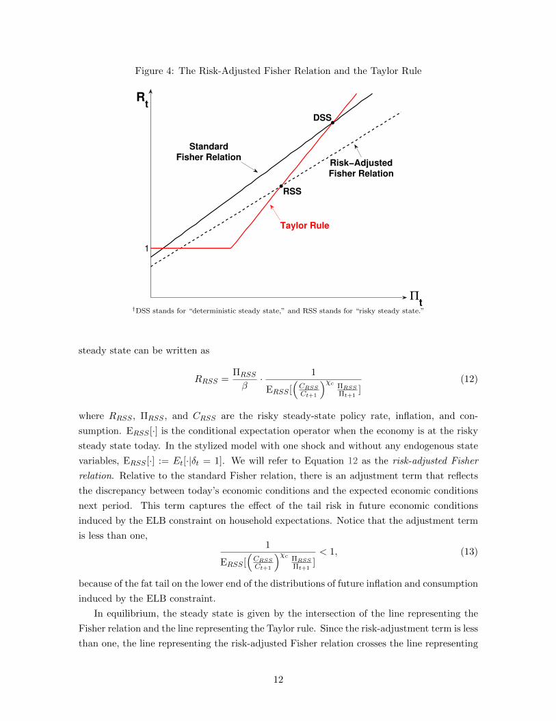
Figure 4: The Risk-Adjusted Fisher Relation and the Taylor Rule

1

RSS

DSS

Πt

Rt

Risk−AdjustedFisher Relation

StandardFisher Relation

Taylor Rule

†DSS stands for “deterministic steady state,” and RSS stands for “risky steady state.”

steady state can be written as

RRSS =ΠRSS

β· 1

ERSS [(CRSSCt+1

)χc ΠRSSΠt+1

](12)

where RRSS , ΠRSS , and CRSS are the risky steady-state policy rate, inflation, and con-

sumption. ERSS [·] is the conditional expectation operator when the economy is at the risky

steady state today. In the stylized model with one shock and without any endogenous state

variables, ERSS [·] := Et[·|δt = 1]. We will refer to Equation 12 as the risk-adjusted Fisher

relation. Relative to the standard Fisher relation, there is an adjustment term that reflects

the discrepancy between today’s economic conditions and the expected economic conditions

next period. This term captures the effect of the tail risk in future economic conditions

induced by the ELB constraint on household expectations. Notice that the adjustment term

is less than one,1

ERSS [(CRSSCt+1

)χc ΠRSSΠt+1

]< 1, (13)

because of the fat tail on the lower end of the distributions of future inflation and consumption

induced by the ELB constraint.

In equilibrium, the steady state is given by the intersection of the line representing the

Fisher relation and the line representing the Taylor rule. Since the risk-adjustment term is less

than one, the line representing the risk-adjusted Fisher relation crosses the line representing

12

the Taylor rule at a point below the line for the standard Fisher relation crosses it, as shown

in Figure 4. Thus, inflation and the policy rate are lower at the risky steady state than at

the deterministic steady state.6

4 The Risky Steady State in an Empirical Model with the

ELB

We now quantify the magnitude of the wedge between the deterministic and risky steady

states in an empirically rich model calibrated to match key features of the U.S. economy.

4.1 Model

Our empirical model adds four additional features on top of the stylized New Keynesian

model of the previous section: (i) a non-stationary productivity process, (ii) consumption

habits, (iii) sticky wages, and (iv) an interest-rate smoothing term in the interest-rate feed-

back rule. Since these features are standard, we relegate the detailed description of them to

the Appendix B and only show the equilibrium conditions of the model here. Let Yt = YtAt

,

Ct = CtAt

, wt = wtAt

, and λt = λtA−χct

be the stationary representations of output, consumption,

real wage, and marginal utility of consumption, respectively, where At is a (deterministic)

non-stationary productivity path. The stationary equilibrium is characterized by the follow-

ing system of equations:

λt =β

aχcδtRtEtλt+1

(Πpt+1

)−1(14)

λt = (Ct −ζ

aCt−1)−χc (15)

Ntwt

λ−1t

[ϕw

(Πwt

Πw− 1

)Πwt

Πw− (1− θw)− θwN

χnt

λtwt

]=

βϕwaχc−1

δtEtNt+1wt+1

λ−1t+1

(Πwt+1

Πw− 1

)Πwt+1

Πw

(16)

Πwt =

wtwt−1

Πpt (17)

Yt

λ−1t

[ϕp

(Πpt

Πp− 1

)Πpt

Πp− (1− θp)− θpwt

]=

βϕpaχc−1

δtEtYt+1

λ−1t+1

(Πpt+1

Πp− 1

)Πpt+1

Πp(18)

Yt = Ct +ϕp2

[Πpt

Πp− 1

]2

Yt +ϕw2

[Πwt

Πw− 1

]2

wtNt (19)

Yt = Nt (20)

6The other intersection of the risk-adjusted Fisher relation and the Taylor-rule equation indicates that, ina deflationary equilibrium, inflation is higher at the risky steady state than at the deterministic steady state.We have confirmed that this is indeed the case using a semi-loglinear model with a three-state discount rateshock. We will leave an in-depth examination of the risky steady state in a deflationary equilibrium to futureresearch.

13

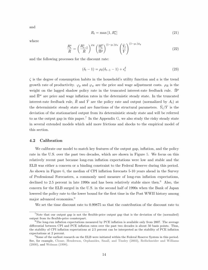
and

Rt = max [1, R∗t ] (21)

where

R∗tR

=

(R∗t−1

R

)ρR (Πpt

Πp

)(1−ρr)φπ(YtY

)(1−ρr)φy

(22)

and the following processes for the discount rate:

(δt − 1) = ρδ(δt−1 − 1) + εδt (23)

ζ is the degree of consumption habits in the household’s utility function and a is the trend

growth rate of productivity. ϕp and ϕw are the price and wage adjustment costs. ρR is the

weight on the lagged shadow policy rate in the truncated interest-rate feedback rule. Πp

and Πw are price and wage inflation rates in the determistic steady state. In the truncated

interest-rate feedback rule, R and Y are the policy rate and output (normalized by At) at

the deterministic steady state and are functions of the structural parameters. Yt/Y is the

deviation of the stationarized output from its deterministic steady state and will be referred

to as the output gap in this paper.7 In the Appendix G, we also study the risky steady state

in several extended models which add more frictions and shocks to the empirical model of

this section.

4.2 Calibration

We calibrate our model to match key features of the output gap, inflation, and the policy

rate in the U.S. over the past two decades, which are shown in Figure 5. We focus on this

relatively recent past because long-run inflation expectations were low and stable and the

ELB was either a concern or a binding constraint to the Federal Reserve during this period.

As shown in Figure 6, the median of CPI inflation forecasts 5-10 years ahead in the Survey

of Professional Forecasters, a commonly used measure of long-run inflation expectations,

declined to 2.5 percent in late 1990s and has been relatively stable since then.8 Also, the

concern for the ELB surged in the U.S. in the second half of 1990s when the Bank of Japan

lowered the policy rate to the lower bound for the first time in the Post WWII history among

major advanced economies.9

We set the time discount rate to 0.99875 so that the contribution of the discount rate to

7Note that our output gap is not the flexible-price output gap that is the deviation of the (normalied)output from its flexible-price counterpart.

8The long-run inflation expectations measured by PCE inflation is available only from 2007. The averagedifferential between CPI and PCE inflation rates over the past two decades is about 50 basis points. Thus,the stability of CPI inflation expectations at 2.5 percent can be interpreted as the stability of PCE inflationexpectations at 2 percent.

9Some of the earliest research on the ELB were initiated within the Federal Reserve System in this period.See, for example, Clouse, Henderson, Orphanides, Small, and Tinsley (2003), Reifschneider and Williams(2000), and Wolman (1998).

14

Figure 5: Output Gap, Inflation, and Policy Rate†

1995 2000 2005 2010 2015−10

−7.5

−5

−2.5

0

2.5

5Output Gap (%)

Year1995 2000 2005 2010 20150

0.5

1

1.5

2

2.5

3Inflation (Annualized %)

Year1995 2000 2005 2010 20150

1

2

3

4

5

6

7

8Policy Rate (Annualized %)

Year

†The measure of the output gap is based on the FRB/US model and is available upon request. The inflation rate iscomputed as the annualized quarterly percentage change (log difference) in the personal consumption expenditure coreprice index (St. Louis Fed’s FRED). The quarerly average of the (annualized) federal funds rate is used as the measurefor the policy rate (St. Louis Fed’s FRED). Vertical lines mark the year when ELB started binding. Horizontal linesrepresent target values for the respective variables.

Figure 6: Long-Run Inflation Expectations†

1990 1995 2000 2005 2010 20151.5

2

2.5

3

3.5

4

Year

†Calculations based on: Federal Reserve Board, Survey of Professional Forecasters, accessed November 2015,https://www.philadelphiafed.org/research-and-data/real-time-center/survey-of-professional-forecasters/.

the deterministic steady state real rate is 50 basis points. We set the target inflation in the

interest-rate feedback rule to 2 percent as this is the FOMC’s official target rate of inflation.

We set the trend growth rate of productivity to 1.25 percent so that the policy rate is 3.75

percent at the economy’s deterministic steady state.

In the household utility function, the degree of consumption habits, the inverse Frisch

labor elasticity, and the inverse intertemporal elasticity of substitution are set to 0.5, 0.5 and

1, respectively. These are all within the range of standard values found the literature.

15

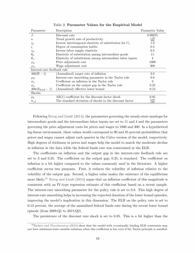
Table 3: Parameter Values for the Empirical Model

Parameter Description Parameter Value

β Discount rate 0.99875a Trend growth rate of productivity 1.25

400χc Inverse intertemporal elasticity of substitution for Ct 1.0ζ Degree of consumption habits 0.5χn Inverse labor supply elasticity 0.5θp Elasticity of substitution among intermediate goods 11θw Elasticity of substitution among intermediate labor inputs 4ϕp Price adjustment cost 1000ϕw Wage adjustment cost 300Interest-rate feedback rule400(Π− 1) (Annualized) target rate of inflation 2.0ρR Interest-rate smoothing parameter in the Taylor rule 0.8φπ Coefficient on inflation in the Taylor rule 3φy Coefficient on the output gap in the Taylor rule 0.25400(RELB − 1) (Annualized) effective lower bound 0.13Shocksρd AR(1) coefficient for the discount factor shock 0.85σε,δ The standard deviation of shocks to the discount factor 0.69

100

Following Erceg and Linde (2014), the parameters governing the steady-state markups for

intermediate goods and the intermediate labor inputs are set to 11 and 4 and the parameters

governing the price adjustment costs for prices and wages to 1000 and 300. In a hypothetical

log-linear environment, these values would correspond to 90 and 85 percent probabilities that

prices and wages cannot adjust each quarter in the Calvo version of the model, respectively.

High degrees of stickiness in prices and wages help the model to match the moderate decline

in inflation in the data while the federal funds rate was constrained at the ELB.

The coefficients on inflation and the output gap in the interest-rate feedback rule are

set to 3 and 0.25. The coefficient on the output gap, 0.25, is standard. The coefficient on

inflation is a bit higher compared to the values commonly used in the literature. A higher

coefficient serves two purposes. First, it reduces the volatility of inflation relative to the

volatility of the output gap. Second, a higher value makes the existence of the equilibrium

more likely.10 Erceg and Linde (2014) argue that an inflation coefficient of this magnitude is

consistent with an IV-type regression estimate of this coefficient based on a recent sample.

The interest-rate smoothing parameter for the policy rule is set to 0.8. This high degree of

interest-rate smoothing helps in increasing the expected duration of the lower bound episodes,

improving the model’s implication in this dimension. The ELB on the policy rate is set to

0.13 percent, the average of the annualized federal funds rate during the recent lower bound

episode (from 2009:Q1 to 2015:Q2).

The persistence of the discount rate shock is set to 0.85. This is a bit higher than the

10Richter and Throckmorton (2015) show that the model with occasionally binding ELB constraints maynot have minimum-state-variable solutions when this coefficient is low even if the Taylor-principle is satisfied.

16

common value of 0.8 used in most existing studies of models with occasionally binding lower

bound constraints.11 A higher persistence of the shock helps in increasing the expected

duration of being at the ELB, as the higher interest-rate smoothing parameter in the policy

rule does. The standard deviation of the discount rate shock is chosen so that the standard

deviation of the policy rate in the model matches with that in the data.

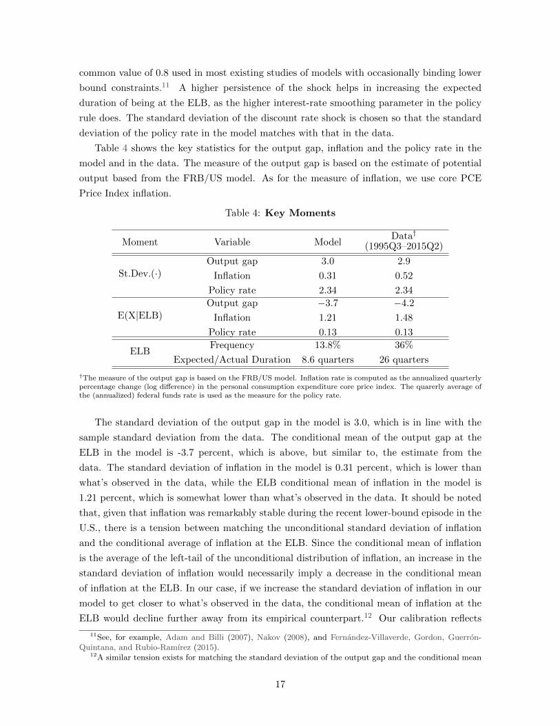
Table 4 shows the key statistics for the output gap, inflation and the policy rate in the

model and in the data. The measure of the output gap is based on the estimate of potential

output based from the FRB/US model. As for the measure of inflation, we use core PCE

Price Index inflation.

Table 4: Key Moments

Moment Variable ModelData†

(1995Q3–2015Q2)

St.Dev.(·)Output gap 3.0 2.9

Inflation 0.31 0.52

Policy rate 2.34 2.34

E(X|ELB)Output gap −3.7 −4.2

Inflation 1.21 1.48

Policy rate 0.13 0.13

ELBFrequency 13.8% 36%

Expected/Actual Duration 8.6 quarters 26 quarters

†The measure of the output gap is based on the FRB/US model. Inflation rate is computed as the annualized quarterlypercentage change (log difference) in the personal consumption expenditure core price index. The quarerly average ofthe (annualized) federal funds rate is used as the measure for the policy rate.

The standard deviation of the output gap in the model is 3.0, which is in line with the

sample standard deviation from the data. The conditional mean of the output gap at the

ELB in the model is -3.7 percent, which is above, but similar to, the estimate from the

data. The standard deviation of inflation in the model is 0.31 percent, which is lower than

what’s observed in the data, while the ELB conditional mean of inflation in the model is

1.21 percent, which is somewhat lower than what’s observed in the data. It should be noted

that, given that inflation was remarkably stable during the recent lower-bound episode in the

U.S., there is a tension between matching the unconditional standard deviation of inflation

and the conditional average of inflation at the ELB. Since the conditional mean of inflation

is the average of the left-tail of the unconditional distribution of inflation, an increase in the

standard deviation of inflation would necessarily imply a decrease in the conditional mean

of inflation at the ELB. In our case, if we increase the standard deviation of inflation in our

model to get closer to what’s observed in the data, the conditional mean of inflation at the

ELB would decline further away from its empirical counterpart.12 Our calibration reflects

11See, for example, Adam and Billi (2007), Nakov (2008), and Fernandez-Villaverde, Gordon, Guerron-Quintana, and Rubio-Ramırez (2015).

12A similar tension exists for matching the standard deviation of the output gap and the conditional mean

17

a compromise of staying reasonably close to the data in these two dimension. It is worth

noting that our estimate of the deflationary bias would be higher if we ignored the observed

stability of inflation at the ELB and adjusted our calibration to match the standard deviation

of inflation, as a lower conditional average of inflation at the ELB induces firms to lower prices

by more when away from the ELB. Thus, our estimate of the deflationary bias can be seen

as a conservative estimate.

As previously mentioned, the standard deviation of the discount rate shock was chosen

so that the standard deviation of the policy rate in the model matches with that in the

data, which is 2.34 percent. The model-implied unconditional probability of being at the

ELB and the expected ELB duration are about 14 percent and 2 years, respectively. While

these numbers are substantially higher than those in other existing models with occasionally

binding ELB constraints, they are substantially lower than the empirical counterparts over

the past two decades in the U.S. In particular, the duration of the recent ELB experience is

seen by the model as surprisingly long. Consistent with this interpretation, the data on liftoff

expectations shows that market participants have underpredicted how long the policy rate

will be kept at the ELB throughout the recent ELB episode, as described in the Appendix E.

4.3 Results

Table 5: The Risky Steady State in the Empirical Model

Inflation Output gap Policy rate

Deterministic steady state 2 0 3.75Risky steady state 1.74 0.30 3.26

(Wedge) (−0.26) (0.30) (−0.49)

Risky steady state w/o the ELB 1.92 0.05 3.56(Wedge) (−0.08) (0.05) (−0.19)

E[·|Rt > RELB] 1.78 0.85 3.85

Table 5 shows the risky and deterministic steady state values of inflation, the output

gap, and the policy rate from our empirical model. For this model, the risky steady state

is computed by simulating the model for a long period while setting the realization of the

exogenous disturbances to zero. All (stationarized) endogenous variables eventually converge

in that simulation, and that point of convergence is the risky state of the economy. By

construction, the deterministic steady state of inflation is given by the target rate of inflation

and the output gap is zero at the deterministic steady state. As explained earlier, parameter

values (β, χc and a) are chosen so that the deterministic steady state of the policy rate is

3.75 percent.

Consistent with our earlier analyses based on a stylized model, inflation and the policy rate

are lower, and the output gap is higher, at the risky steady state than at the deterministic

of the output gap at the ELB, but to a lesser extent.

18

steady state. Inflation falls 26 basis points below the target rate of inflation at the risky

steady state. This is large given the small standard deviation of inflation. The policy rate

at the risky steady state falls 49 basis points below its deterministic counterpart. While this

is a small number relative to its standard deviation, it is nevertheless significant in light of

recent discussions among economists and policymakers regarding the long-run equilibrium

policy rate.13 Finally, the output wedge between the deterministic and risky steady states is

small, with the output gap standing at 0.30 percentage point at the risky steady state.

As explained in the previous section, the discrepancy between the deterministic and risky

steady states is not only driven by the lower bound constraint on policy rates, but is also

affected by other nonlinear features of the model. To isolate the effects of the lower bound

constraint, the fourth line of Table 5 shows the risky steady state of the model without the

lower bound constraint. Inflation, the output gap, and the policy rate are 1.92, 0.05, and 3.56

percent, respectively. Thus, most of the wedge between the deterministic and risky steady

states in the model with the ELB constraint is attributed to the nonlinearity associated with

the ELB constraint, as opposed to other nonlinear features of the model. For inflation, the

ELB risk accounts for 18 basis points of the overall deflationary bias.

4.4 Sensitivity Analyses

4.4.1 Long-Run Interest Rates

There are substantial uncertainties surrounding the level of the long-run real equilib-

rium interest rate. Many economists recently have argued that various structural factors—

including a lower trend growth rate of productivity, demographic trends, and global factors—

have contributed to a persistent downward trend in the long-run equilibrium interest rate.14

A lower long-run equilibrium interest rate means that the probability of hitting the ELB is

higher, which ceteris paribus increases the magnitude of the undershooting of the inflation

target at the risky steady state.

Figure 7 shows how sensitive the risky steady state of our empirical model is to alternative

assumptions about the deterministic steady state interest rate. In this exercise, we vary the

long-run deterministic steady-state policy rate by varying the trend growth rate. As shown

in the top-left panel, the probability of the policy rate being at the ELB increases as the

deterministic steady state policy rate declines. With the deterministic steady state policy

rate at 3.35 percent, the probability of being at the ELB is approximately 25 percent. A

higher probability of being at the ELB increases the wedge between the deterministic and

risky steady states. With the deterministic steady state policy rate at 3.35 percent, the risky

steady state inflation, output, and the policy rates are 1.47 percent, 0.64 percent, and 2.39

percent.15 Since the risky steady state does not depend on the deterministic steady state

13See, for example, Hamilton, Harris, Hatzius, and West (2015) and Rachel and Smith (2015).14See, for example, the Council of Economic Advisers (2015) and IMF (2014).15Note that an increase in the output gap does not necessarily mean an increase in the level of output

19

Figure 7: Long-Run Interest Rates and the Risky Steady State†

3.35 3.5 3.75 4 4.256

10

14

18

22

26

DSS Policy Rate

Probability of being at the ELB

3.35 3.5 3.75 4 4.25

1.5

1.6

1.7

1.8

1.9

2

DSS Policy Rate

RSS Inflation

With ELB Constraint

Without ELB Constraint

3.35 3.5 3.75 4 4.250

0.1

0.2

0.3

0.4

0.5

0.6

0.7

DSS Policy Rate

RSS Output Gap

3.35 3.5 3.75 4 4.252

2.5

3

3.5

4

4.5

DSS Policy Rate

RSS Policy Rate

†DSS stands for “deterministic steady state,” and RSS stands for “risky steady state.” Vertical lines mark the DSSpolicy rate in the baseline calibration.

policy rate in the model without the ELB constraint, as shown in the dashed lines, a large

fraction of the overall wedge is explained by the ELB risk when the deterministic steady state

policy rate is lower. For inflation, the ELB risk accounts for 45 basis points of the overall

deflationary bias of 53 basis points.16

4.4.2 Policy Parameters

We have shown that, at the risky steady state, inflation falls below the target rate of 2

percent by a nontrivial amount in our empirical model. In our model where the prices and

wages are indexed to the target rate of inflation, such undershooting of the inflation target

is undesirable. A natural question to ask is what the central bank can do to mitigate the

deflationary bias.17

Figure 8 showd how the probability of being at the ELB and the risky steady-state

because output measures are stationarized by the trend growth rate.16Hamilton, Harris, Hatzius, and West (2015) argue that any value between 0 and 2 percent is a plausible

value for the long-run real rate. Thus, the long-run nominal rate of 2.39 percent—or equivalently, the long-runreal rate of 0.39 percent—in this example is within their plausible range.

17In this paper, we examine this issue only in the context of a Taylor-type rule. Under price-level targetingor nominal income targeting, which are known to mitigate the decline in inflation at the ELB, the deflationarybias is likely to be smaller than under a conventional Taylor-type rule.

20

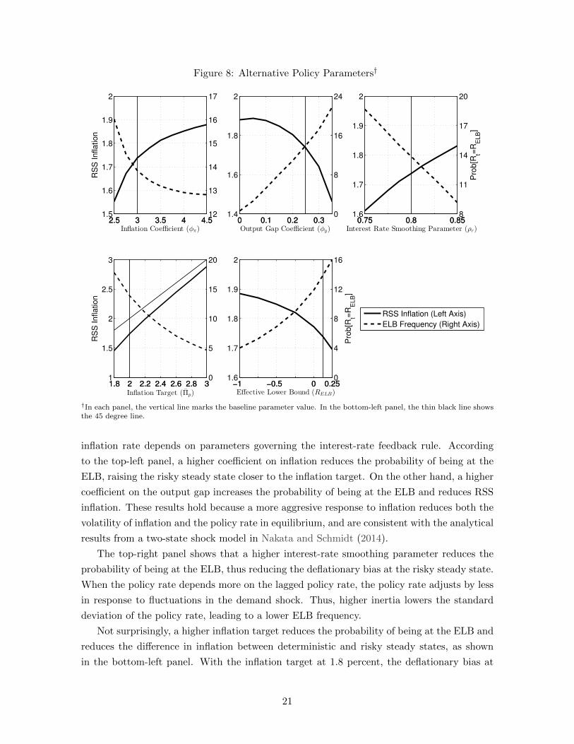
Figure 8: Alternative Policy Parameters†

2.5 3 3.5 4 4.51.5

1.6

1.7

1.8

1.9

2

Inflation Coefficient (φπ)

RS

S I

nfla

tio

n

2.5 3 3.5 4 4.512

13

14

15

16

17

RSS Inflation (Left Axis)

ELB Frequency (Right Axis)

0 0.1 0.2 0.31.4

1.6

1.8

2

Output Gap Coefficient (φy)0 0.1 0.2 0.3

0

8

16

24

0.75 0.8 0.851.6

1.7

1.8

1.9

2

Interest Rate Smoothing Parameter (ρr)0.75 0.8 0.85

8

11

14

17

20

Pro

b[R

t=R

ELB]

1.8 2 2.2 2.4 2.6 2.8 31

1.5

2

2.5

3

Inflation Target (Πp)

RS

S I

nfla

tio

n

1.8 2 2.2 2.4 2.6 2.8 30

5

10

15

20

−1 −0.5 0 0.251.6

1.7

1.8

1.9

2

Effective Lower Bound (RELB)−1 −0.5 0 0.25

0

4

8

12

16

Pro

b[R

t=R

ELB]

†In each panel, the vertical line marks the baseline parameter value. In the bottom-left panel, the thin black line showsthe 45 degree line.

inflation rate depends on parameters governing the interest-rate feedback rule. According

to the top-left panel, a higher coefficient on inflation reduces the probability of being at the

ELB, raising the risky steady state closer to the inflation target. On the other hand, a higher

coefficient on the output gap increases the probability of being at the ELB and reduces RSS

inflation. These results hold because a more aggresive response to inflation reduces both the

volatility of inflation and the policy rate in equilibrium, and are consistent with the analytical

results from a two-state shock model in Nakata and Schmidt (2014).

The top-right panel shows that a higher interest-rate smoothing parameter reduces the

probability of being at the ELB, thus reducing the deflationary bias at the risky steady state.

When the policy rate depends more on the lagged policy rate, the policy rate adjusts by less

in response to fluctuations in the demand shock. Thus, higher inertia lowers the standard

deviation of the policy rate, leading to a lower ELB frequency.

Not surprisingly, a higher inflation target reduces the probability of being at the ELB and

reduces the difference in inflation between deterministic and risky steady states, as shown

in the bottom-left panel. With the inflation target at 1.8 percent, the deflationary bias at

21

the risky steady state is about 35 basis points. With the inflation target at 3 percent, the

deflationary bias at the risky steady state is about 12 basis points. This exercise demonstrates

the importance of taking into account the lower bound risk in the cost-benefit analysis of

raising the inflation target.18 Finally, the last panel demonstrates that, if the effective lower

bound is lower, the ELB binds less often and thus the deflationary bias is lower at the risky

steady state.

5 Discussion

Why should we care about what a theoretical model has to say about the ELB risk and

the resulting deflationary bias? In this section, we argue that we should care about it for

two reasons. First, the model with the ELB risk is consistent with the undershooting of the

inflation target observed in some economies even before the policy rate became constrained

by the ELB constraint. Second, the model with the ELB risk provides a cautionary tale for

policymakers aiming to achieve their inflation objectives in the current environment of low

long-run equilibrium real interest rates.

5.1 Low inflation before the Great Recession

Figure 9 shows the conditional averages of inflation over the past two decades when

policy rates were not constrained by the ELB in four advanced economies—economies that

have recently faced the ELB constraint for the first time since WWII and target 2% inflation

symmetrically. According to the figure, the conditional averages of inflation away from the

ELB are below the target rate of 2 percent in all these economies. In the U.S and Canada,

inflation averaged about 20 and 40 basis points below 2 percent while the policy rate was

not constrained by the ELB. In the UK, the conditional average of inflation away from the

ELB is 60 basis points below 2 percent. In Sweden, the average inflation rate is below 1

percent while the policy rate was above the ELB. In the Appendix F, we show that the

undershooting of the inflation target is robust to alternative starting dates of sample and the

difference between the conditional average and the target rate is statistically significant for

all four economies.

While there are many explanations for this systematic undershooting of the inflation

targets before the ELB became a binding constraint—such as positive supply shocks from

emerging economies and persistent slack in the economies—it is interesting to note that this

undershooting is consistent with the prediction of the model with the ELB risk. As argued

earlier, one key prediction of the model with the ELB risk is that the conditional average

of inflation away from the ELB falls below the target rate of 2 percent, provided that the

probability of being at the ELB is sufficiently high. In our empirical model, the deflationary

18The computation of the optimal inflation target is often conducted under the assumption of perfect-foresight. See, for example, Williams (2009) and Coibion, Gorodnichenko, and Wieland (2012).

22

Figure 9: Conditional Averages of Inflation Away From the ELB†

0.5

1

1.5

2

UnitedStates

Canada UnitedKingdom

Sweden

† The figure shows the average of the annualied quarterly inflation rate over the past two decades (since 1995Q3) foreach country during non-ELB quarters—when the country’s policy rate was not constrained by the ELB. For the U.S,the measure of inflation is based on core PCE Price Index. For other economies, the measure of inflation is ased on coreCPI Index. ELB-binding quarters are from 2009Q1 to present in the U.S., from 2009:Q2 to 2010:Q1 in Canada, from2009:Q2 to present in UK, from 2009:Q4 to 2010:Q2 and from 2014:Q4 to present in Sweden.Data for inflation sourced from: for United States, Federal Reserve Bank of St. Louis, Personal Consumption Expendi-tures: Chain-type Price Index Less Food and Energy, accessed December 2015, https://research.stlouisfed.org/fred2/;for all other countries, OECD (2015), Inflation (Core CPI) (indicator), accessed November 2015, DOI: 10.1787/eee82e6e-en.

bias is indeed large enough to push the conditional average of inflation away from the ELB

below the inflation target, as shown in the last row of Table 5. 19

Since the risk of hitting the ELB was widely seen as unlikely before the Great Recession,

we do not think that this ELB risk is a good explanation for the target undershooting in pre-

ELB era in reality. However, we think the ability of our model to generate the undershooting

in pre-ELB era is attractive. As explained in Section 3.3 and Appendix H, a version of our

model with the ELB constraint, but without the ELB risk, does not have this feature. More

research is certainly needed to better understand the sources of low inflation in advanced

economies and what policymakers can do to address this problem.

5.2 An implication for the future

It is quite likely that the perceived probability of hitting the ELB is higher now than

before the Great Recession. The Great Recession made clear that the economy can be hit by

19Note that this undershooting of the inflation target while the policy rate is above the ELB is not consistentwith the deflationary steady state of the sticky-price economy (Benhabib, Schmitt-Grohe, and Uribe (2001)and Armenter (2014)). In the deflationary steady state, inflation is below the target, but the policy rate is atthe ELB.

23

shocks that are substantially larger than the macro shocks that hit the economy during the

Great Moderation. Moreover, several years of disappointing output growth in the aftermath

of the Great Recession have led many analysts to revise down their estimates of the trend

growth rate of productivity and long-run nominal interest rates. As shown in Section 4.4.1 a

lower long-run equilibrium interest rate would imply a higher ELB frequency.

As our earlier sensitivity analyses demonstrated, the size of the deflationary bias at the

risky steady state increases with the probability of being at the ELB. Thus, our model

provides a cautionary tale for policymakers: Achieving the target rate of inflation may have

become more difficult now than before the Great Recession if the recent ELB experience has

led the private sector to revise its assessment of the likelihood of ELB events.

6 Conclusion

In this paper, we have examined the implications of the ELB risk—the possibility that

the policy rate will be constrained by the ELB in the future—for the economy when the

policy rate is currently not constrained. Using an empirically rich DSGE model calibrated to

capture key features of the U.S. economy over the past two decades, we have shown that the

ELB risk causes inflation to fall below the target rate of 2 percent by about 20 basis points

at the risky steady state. The deflationary bias induced by the ELB risk at the risky steady

state can be as much as 45 basis points under alternative plausible assumptions about the

long-run growth rate of the economy and monetary policy parameters. Our analysis suggests

that achieving the inflation target may be more difficult now than before the Great Recession,

if the recent lower bound episode has led the private sector to increase their assessment of

the ELB risk.

References

Adam, K., and R. Billi (2007): “Discretionary Monetary Policy and the Zero Lower Bound on

Nominal Interest Rates,” Journal of Monetary Economics, 54(3), 728–752.

Armenter, R. (2014): “The perils of nominal targets,” Working Paper 14-2, Federal Reserve Bank

of Philadelphia.

Aruoba, B. S., P. Cuba-Borda, and F. Schorfheide (2014): “Macroeconomic Dynamics Near

the ZLB: a Tale of Two Countries,” Working Paper.

Benhabib, J., S. Schmitt-Grohe, and M. Uribe (2001): “The Perils of Taylor Rules,” Journal

of Economic Theory, 96(1-2), 40–69.

Benigno, G., and L. Fornaro (2015): “Stagnation Traps,” Working Paper.

Bullard, J. (2010): “Seven Faces of “The Peril”,” Federal Reserve Bank of St. Louis Review, 92(5),

339–52.

24

Christiano, L., M. Eichenbaum, and S. Rebelo (2011): “When is the Government Spending

Multiplier Large?,” Journal of Political Economy, 119(1), 78–121.

Christiano, L. J., and J. D. M. Fisher (2000): “Algorithms for solving dynamic models with

occasionally binding constraints,” Journal of Economic Dynamics and Control, 24(8), 1179–1232.

Clouse, J., D. Henderson, A. Orphanides, D. H. Small, and P. A. Tinsley (2003): “Mone-

tary Policy When the Nominal Short-Term Interest Rate is Zero,” The B.E. Journal of Macroeco-

nomics, 3(1), 1–65.

Coenen, G., A. Orphanides, and V. Wieland (2004): “Price Stability and Monetary Policy

Effectiveness when Nominal Interest Rates are Bounded at Zero,” B.E. Journal of Macroeconomics:

Advances in Macroeconomics, 4(1), 1–25.

Coeurdacier, N., H. Rey, and P. Winant (2011): “The Risky Steady State,” American Economic

Review, 101(3), 398–401.

Coibion, O., Y. Gorodnichenko, and J. Wieland (2012): “The Optimal Inflation Rate in New

Keynesian Models: Should Central Banks Raise Their Inflation Targets in Light of the ZLB?,”

Review of Economic Studies, 79(4), 1371–1406.

de Groot, O. (2013): “Computing the risky steady state of DSGE models,” Economics Letters,

120(3), 566–569.

(2014): “The Risk Channel of Monetary Policy,” International Journal of Central Banking,

10(2), 115–160.

Devereux, M. B., and A. Sutherland (2011): “Country Portfolios In Open Economy Macro-

Models,” Journal of the European Economic Association, 9(2), 337–369.

Eggertsson, G., and M. Woodford (2003): “The Zero Bound on Interest Rates and Optimal

Monetary Policy,” Brookings Papers on Economic Activity, 34(1), 139–235.

Eggertsson, G. B., and N. R. Mehrotra (2014): “A Model of Secular Stagnation,” NBER

Working Paper Series 20574, National Bureau of Economic Research.

Erceg, C. J., and J. Linde (2014): “Is There a Fiscal Free Lunch in a Liquidity Trap?,” Journal

of the European Economic Association, 12(1), 73–107.

Fernandez-Villaverde, J., G. Gordon, P. A. Guerron-Quintana, and J. Rubio-Ramırez

(2015): “Nonlinear Adventures at the Zero Lower Bound,” Journal of Economic Dynamics and

Control, 57, 182–204.

Gavin, W. T., B. D. Keen, A. W. Richter, and N. A. Throckmorton (2015): “The Zero

Lower Bound, the Dual Mandate, and Unconventional Dynamics,” Journal of Economic Dynamics

and Control, 55, 14–38.

Gertler, M., N. Kiyotaki, and A. Queralto (2012): “Financial Crises, Bank Risk Exposure

and Government Financial Policy,” Journal of Monetary Economics, 59, 17–34.

25

Gust, C., D. Lopez-Salido, and M. Smith (2012): “The Empirical Implications of the Interest-

Rate Lower Bound,” Finance and Economics Discussion Series 2012-83, Board of Governors of the

Federal Reserve System (U.S.).

Hamilton, J. D., E. Harris, J. Hatzius, and K. D. West (2015): “The Equilibrium Real Funds

Rate: Past, Present and Future,” Working Paper.

IMF (2014): “World Economic Outlook April 2014,” .

Keen, B., A. Richter, and N. A. Throckmorton (2015): “Forward Guidance and the State of

the Economy,” Working Paper.

Maliar, L., and S. Maliar (2015): “Merging Simulation and Projection Approaches to Solve High-

Dimensional Problems with an Application to a New Keynesian Model,” Quantitative Economics,

6(1), 1–47.

Meyer-Gohde, A. (2015): “Risk-Sensitive Linear Approximations,” Working Paper.

Nakata, T. (2013a): “Optimal Fiscal and Monetary Policy With Occasionally Binding Zero Bound

Constraints,” Finance and Economics Discussion Series 2013-40, Board of Governors of the Federal

Reserve System (U.S.).

(2013b): “Uncertainty at the Zero Lower Bound,” Finance and Economics Discussion Series

2013-09, Board of Governors of the Federal Reserve System (U.S.).

Nakata, T., and S. Schmidt (2014): “Conservatism and Liquidity Traps,” Finance and Economics

Discussion Series 2014-105, Board of Governors of the Federal Reserve System (U.S.).

Nakov, A. (2008): “Optimal and Simple Monetary Policy Rules with Zero Floor on the Nominal

Interest Rate,” International Journal of Central Banking, 4(2), 73–127.

Rachel, L., and T. D. Smith (2015): “Secular Drivers of the Global Real Interest Rate,” Staff

Working Paper 571, Bank of England.

Reifschneider, D., and J. C. Williams (2000): “Three Lessons for Monetary Policy in a Low-

Inflation Era,” Journal of Money, Credit and Banking, 32(4), 936–966.

Richter, A. W., and N. A. Throckmorton (2015): “The Zero Lower Bound: Frequency, Du-

ration, and Numerical Convergence,” B.E. Journal of Macroeconomics: Contributions, 15(1), 157–

182.

Schmidt, S. (2013): “Optimal Monetary and Fiscal Policy with a Zero Bound on Nominal Interest

Rates,” Journal of Money, Credit and Banking, 45(7), 1335–1350.

Schmitt-Grohe, S., and M. Uribe (2013): “The Making of a Great Contraction with a Liquidity

Trap and a Jobless Recovery,” Working Paper.

the Council of Economic Advisers (2015): “Long-Term Interest Rates: A Survey,” .

Tille, C., and E. van Wincoop (2010): “International Capital Flows,” Journal of International

Economics, 80(2), 157–175.

26

Williams, J. C. (2009): “Heeding Daedalus: Optimal Inflation and the Zero Lower Bound,” Brook-

ings Papers on Economic Activity, 2, 1–49.

Wolman, A. L. (1998): “Staggered Price Setting and the Zero Bound on Nominal Interest Rates,”

Federal Reserve Bank of Richmond Economic Quarterly, 84(4), 1–24.

27

For Online Publication: Technical Appendix

A Details of the Stylized Model

This section describes a stylized DSGE model with a representative household, a final goodproducer, a continuum of intermediate goods producers with unit measure, and governmentpolicies.

A.1 Household

The representative household chooses its consumption level, amount of labor, and bondholdings so as to maximize the expected discounted sum of utility in future periods. As iscommon in the literature, the household enjoys consumption and dislikes labor. Assumingthat period utility is separable, the household problem can be defined by

maxCt,Nt,Bt

E1

∞∑t=1

βt−1[ t−1∏s=0

δs

][C1−χct

1− χc− N1+χn

t

1 + χn

](A.1)

subject to the budget constraint

PtCt +R−1t Bt ≤WtNt +Bt−1 + PtΦt (A.2)

or equivalently

Ct +BtRtPt

≤ wtNt +Bt−1

Pt+ Φt (A.3)

where Ct is consumption, Nt is the labor supply, Pt is the price of the consumption good, Wt

(wt) is the nominal (real) wage, Φt is the profit share (dividends) of the household from theintermediate goods producers, Bt is a one-period risk free bond that pays one unit of moneyat period t+1, and R−1

t is the price of the bond.

The discount rate at time t is given by βδt where δt is the discount factor shock alteringthe weight of future utility at time t+1 relative to the period utility at time t. This shockfollows an AR(1) process:

δt − 1 = ρ(δt−1 − 1) + εt, εt ∼ N(0, σε) (A.4)

This increase in δt is a preference imposed by the household to increase the relative valuationof future utility flows, resulting in decreased consumption today (when considered in theabsence of changes in the nominal interest rate).

A.2 Firms

There is a final good producer and a continuum of intermediate goods producers indexedby i ∈ [0, 1]. The final good producer purchases the intermediate goods Yi,t at the intermedi-ate price Pi,t and aggregates them using CES technology to produce and sell the final good

28

Yt to the household and government at price Pt. Its problem is then summarized as

maxYi,t,i∈[0,1]

PtYt −∫ 1

0Pi,tYi,tdi (A.5)

subject to the CES production function

Yt =[ ∫ 1

0Y

θ−1θ

i,t di] θθ−1

. (A.6)

Intermediate goods producers use labor to produce the imperfectly substitutable intermedi-ate goods according to a linear production function (Yi,t = Ni,t) and then sell the product tothe final good producer. Each firm maximizes its expected discounted sum of future profits20

by setting the price of its own good. We can assume that each firm receives a productionsubsidy τ so that the economy is fully efficient in the steady state.21 In our baseline, however,we set τ = 0. Price changes are subject to quadratic adjustment costs.

maxPi,t

E1

∞∑t=1

βt−1[ t−1∏s=0

δs

]λt

[Pi,tYi,t − (1− τ)WtNi,t − Pt

ϕ

2[Pi,t

Pi,t−1Π− 1]

2Yt

](A.7)

such that

Yi,t =

[Pi,tPt

]−θYt.

22 (A.8)

λt is the Lagrange multiplier on the household’s budget constraint at time t and βt−1[∏t−1

s=0 δs

]λt

is the marginal value of an additional profit to the household. The positive time zero priceis the same across firms (i.e. Pi,0 = P0 > 0).

A.3 Government policies

It is assumed that the monetary authority determines nominal interest rates according toa Taylor rule

Rt = max

[1,

Π

β

(Πt

Π

)φπ (YtY

)φy](A.9)

where Πt = PtPt−1

and Y is the steady state level of output. This equation will be modified inorder to do an extensive sensitivity analysis of policy inertia and other rule specifications.

20Each period, as it is written below, is in nominal terms. However, we want each period’s profits in realterms so the profits in each period must be divided by that period’s price level Pt which we take care of furtheralong in the document.

21(θ− 1) = (1− τ)θ which implies zero profits in the zero inflation steady state. In a welfare analysis, thiswould extract any inflation bias from the second-order approximated objective welfare function. τ thereforerepresents the size of a steady state distortion (see Chapter 5 Appendix, Galı (2008)).

22This expression is derived from the profit maximizing input demand schedule when solving for the finalgood producer’s problem above. Plugging this expression back into the CES production function implies that

the final good producer will set the price of the final good Pt =[ ∫ 1

0P 1−θi,t di

] 11−θ

.

29

A.4 Market clearing conditions

The market clearing conditions for the final good, labor and government bond are givenby

Yt = Ct +

∫ 1

0

ϕ

2

[ Pi,tPi,t−1Π

− 1]2Ytdi (A.10)

Nt =

∫ 1

0Ni,tdi (A.11)

andBt = 0. (A.12)

A.5 Recursive equilibrium

Given P0 and a two-state Markov shock process establishing δt and γt, an equilibriumconsists of allocations {Ct, Nt, Ni,t, Yt, Yi,t, Gt}∞t=1, prices {Wt, Pt, Pi,t}∞t=1, and a policy in-strument {Rt}∞t=1 such that (i) given the determined prices and policies, allocations solve theproblem of the household, (ii) Pi,t solves the problem of firm i, (iii) Rt follows a specifiedrule, and (iv) all markets clear.

Combining all of the results from (i)-(v), a symmetric equilibrium can be characterizedrecursively by {Ct, Nt, Yt, wt,Πt, Rt}∞t=1 satisfying the following equilibrium conditions:

C−χct = βδtRtEtC−χct+1 Π−1

t+1 (A.13)

wt = Nχnt Cχct (A.14)

YtCχct

[ϕ

(Πt

Π− 1

)Πt

Π− (1− θ)− θ(1− τ)wt

]= βδtEt

Yt+1

Cχct+1

ϕ

(Πt+1

Π− 1

)Πt+1

Π(A.15)

Yt = Ct +ϕ

2

[Πt

Π− 1

]2

Yt (A.16)

Yt = Nt (A.17)

Rt = max

[1,

Π

β

(Πt

Π

)φπ (YtY

)φy](A.18)

Equation A.13 is the consumption Euler equation, Equation A.14 is the intratemporal op-timality condition of the household, Equation A.15 is the optimal condition of the inter-mediate good producing firms (forward-looking Phillips Curve) relating today’s inflation toreal marginal cost today and expected inflation tomorrow, Equation A.16 is the aggregateresource constraint capturing the resource cost of price adjustment, and Equation A.17 is theaggregate production function. Equation A.18 is the interest-rate feedback rule.

B Details of the Empirical Model

This section describes an extension of the stylized model with a representative household,a final good producer, a continuum of intermediate goods producers with unit measure, andthe government.

30

B.1 Household markets

B.1.1 Labor packer

The labor packer buys labor Nh,t from households at their monopolistic wage Wh,t andresells the packaged labor Nt to intermediate goods producers at Wt. The problem can bewritten as

maxNh,t,h∈[0,1]

WtNt −∫ 1

0Wh,tNh,tdf (B.1)

subject to the following CES technology

Nt =

[∫ 1

0N

θw−1θw

h,t dh

] θw

θw−1

. (B.2)

The first order condition implies a labor demand schedule

Nh,t =

[Wh,t

Wt

]−θwNt.

23 (B.3)

θw is the wage markup parameter.

B.1.2 Household

The representative household chooses its consumption level, amount of labor, and bondholdings so as to maximize the expected discounted sum of utility in future periods. As iscommon in the literature, the household enjoys consumption and dislikes labor. Assumingthat period utility is separable, the household problem can be defined by

maxCh,t,wh,t,Bh,t

E1

∞∑t=1

βt−1

[t−1∏s=0

δs

][(Ch,t − ζCat−1)1−χc

1− χc−A1−χc

t

N1+χnh,t

1 + χn

](B.4)

subject to the budget constraint

PtCh,t+R−1t Bh,t ≤Wh,tNh,t−Wt

ϕw2

[Wh,t

aWh,t−1

(Πw)1−ιw (Πw

t−1

)ιw − 1

]2

Nt+Bh,t−1+PtΦt−PtTt

(B.5)or equivalently

Ch,t+Bh,tRtPt

≤ wh,tNh,t−wtϕw2

[wh,t

awh,t−1

Πpt(

Πw)1−ιw (Πw

t−1

)ιw − 1

]2

Nt+Bh,t−1

Pt+Φt−Tt (B.6)

and subject to the labor demand schedule

Nh,t =

[Wh,t

Wt

]−θwNt. (B.7)

23This implies that the labor packer will set the wage of the packaged labor to Wt =[∫ 1

0W 1−θwh,t dh

] 11−θw

.

31

–or equivalently

Nh,t =

[wh,twt

]−θwNt. (B.8)

where Ch,t is the household’s consumption, Nh,t is the labor supplied by the household, Pt isthe price of the consumption good, Wh,t (wh,t) is the nominal (real) wage set by the house-hold, Wt (wt) is the market nominal (real) wage, Φt is the profit share (dividends) of thehousehold from the intermediate goods producers, Bh,t is a one-period risk free bond thatpays one unit of money at period t+1, Tt are lump-sum taxes or transfers, and R−1

t is theprice of the bond. Cat−1 represents the aggregate consumption level from the previous periodthat the household takes as given. The parameter 0 ≤ ζ < 1 measures how important theseexternal habits are to the household. Because we are including wage indexation, measured bythe parameter ιw, we assume the household takes as given the previous period wage inflation,Πwt−1, where Πw

t = WtaWt−1

= wtPtawt−1Pt−1

= wtawt−1

Πpt .

The discount rate at time t is given by βδt where δt is the discount factor shock alteringthe weight of future utility at time t+1 relative to the period utility at time t. δt is assumedto follow an AR(1) process

(δt − 1) = ρδ(δt−1 − 1) + εδt ∀t ≥ 2 (B.9)

and δ1 is given. The innovation εδt is normally distributed with mean zero and standard devi-ation σδ. It may therefore be interpreted that an increase in δt is a preference imposed by thehousehold to increase the relative valuation of the future utility flows, resulting in decreasedconsumption today (when considered in the absence of changes in the nominal interest rate).

At is a non-stationary total factor productivity shock that also augments labor in the utilityfunction in order to accommodate the necessary stationarization of the model later on. Seethe next section for more details on this process.

B.2 Producers

B.2.1 Final good producer

The final good producer purchases the intermediate goods Yf,t at the intermediate pricePf,t and aggregates them using CES technology to produce and sell the final good Yt to thehousehold and government at price Pt. Its problem is then summarized as

maxYf,t,f∈[0,1]

PtYt −∫ 1

0Pf,tYf,tdi (B.10)

subject to the CES production function

Yt =

[∫ 1

0Y

θp−1θp

f,t di

] θp

θp−1

. (B.11)

θp is the price markup parameter.

32

B.2.2 Intermediate goods producers

There is a continuum of intermediate goods producers indexed by f ∈ [0, 1]. Intermediategoods producers use labor to produce the imperfectly substitutable intermediate goods ac-cording to a linear production function (Yf,t = AtNf,t) and then sell the product to the finalgood producer. Each firm maximizes its expected discounted sum of future profits24 by set-ting the price of its own good. Any price changes are subject to quadratic adjustment costs.ϕp will represent an obstruction of price adjustment, the firm indexes for prices—measuredby ιp—and takes as given previous period inflation Πp

t−1, and Πp represents the monetaryauthority’s inflation target.

maxPf,t

E1

∞∑t=1

βt−1

[t−1∏s=0

δs

]λt

[Pf,tYf,t −WtNf,t − Pt

ϕp2

[Pf,t(

Πp)1−ιp (Πp

t−1

)ιp Pf,t−1

− 1]2Yt

](B.12)

such that

Yf,t =

[Pf,tPt

]−θpYt.

25 (B.13)

λt is the Lagrange multiplier on the household’s budget constraint at time t and βt−1[∏t−1

s=0 δs

]λt

is the marginal value of an additional profit to the household. The positive time zero priceis the same across firms (i.e. Pi,0 = P0 > 0).

At represents total factor productivity which follows a random walk with drift:

ln(At) = ln(a) + ln(At−1) + at. (B.14)

a is the unconditional rate of growth of productivity. at is a productivity shock following anAR(1) process:

ln(at) = ρaln(at−1) + εAt . (B.15)

where εAt is normally distributed with mean zero and standard deviation σA. This growthfactor will imply that some of the variables will acquire a unit root, meaning the model willhave to be stationarized. Monetary policy will also have to accommodate this growth factoras well.

B.3 Government policies

It is assumed that the monetary authority determines nominal interest rates according toa truncated notional inertial Taylor rule augmented by a speed limit component.

Rt = max [1, R∗t ] (B.16)

24NOTE: Each period, as it is written below, is in nominal terms. However, we want each period’s profitsin real terms so the profits in each period must be divided by that period’s price level Pt which we take careof further along in the document.

25This expression is derived from the profit maximizing input demand schedule when solving for the finalgood producer’s problem above. Plugging this expression back into the CES production function implies that

the final good producer will set the price of the final good Pt =[∫ 1

0P 1−θpf,t di

] 11−θp

.

33

whereR∗tR

=

(R∗t−1

R

)ρR (Πpt

Πp

)(1−ρr)φπ ( YtAtY

)(1−ρr)φyexp(εRt ) (B.17)

where Πpt = Pt

Pt−1is the inflation rate between periods t− 1 and t, R = Πpaχc

β (see the section

on stationarization to see why), and εRt represents white noise monetary policy shocks withmean zero and standard deviation σR.

B.4 Market clearing conditions

The market clearing conditions for the final good, labor and government bond are given by

Yt = Ct +

∫ 1

0

ϕp2

[Pf,t(

Πp)1−ιp (Πp

t−1

)ιp Pf,t−1

− 1

]2

Ytdf + ...

...+

∫ 1

0wtϕw2

[wh,t

awh,t−1

Πpt(

Πw)1−ιw (Πw

t−1

)ιw − 1

]2

Ntdh

(B.18)

Nt =

∫ 1

0Nf,tdi (B.19)

Cat = Ct =

∫ 1

0Ch,tdh (B.20)

and

Bt =

∫ 1

0Bh,tdh = 0. (B.21)

B.5 An equilibrium

Given P0 and stochastic processes for δt, an equilibrium consists of allocations {Ct, Nt,Nf,t, Yt, Yf,t, Gt}∞t=1, prices {Wt, Pt, Pf,t}∞t=1, and a policy instrument {Rt}∞t=1 such that

(i) allocations solve the problem of the household given prices and policies

∂Ch,t : (Ch,t − ζCat−1)−χc − λt = 0 (B.22)

∂wh,t : θwA1−χct

N1+χnt

wt

(wh,twt

)−θw(1+χn)−1

+(1− θw)λt

(wh,twt

)−θwNt

−λtwtϕw

(wh,t

awh,t−1

Πpt(

Πw)1−ιw (Πw

t−1

)ιw − 1

)Nt

Πpt

awh,t−1

(Πw)1−ιw (Πw

t−1

)ιw+βδtEtλt+1wt+1ϕw

(wh,t+1

awh,t

Πpt+1(

Πw)1−ιw (Πw

t )ιw− 1

)Nt+1

wh,t+1

aw2h,t

Πpt+1(

Πw)1−ιw (Πw

t )ιw= 0

(B.23)

∂Bh,t : − λtRtPt

+ βδtEtλt+1

Pt+1= 0 (B.24)

34

(ii) Pf,t solves the problem of firm i

By making the appropriate substitution (the intermediate goods producer’s constraints inplace of Yf,t and subsequently in for Nf,t) and by dividing each period’s profits by that pe-riod’s price level Pt so as to put profits in real terms (and thus make profits across periodscomparable) we get the following:

∂Pf,t : λtYtPt

[ Pt(Πp)1−ιp (Πp

t−1

)ιp Pf,t−1

ϕp

(Pf,t(

Πp)1−ιp (Πp

t−1

)ιp Pf,t−1

− 1

)− (1− θp)

(Pf,tPt

)−θp

−θpwtAt

(PtPf,t

)1+θp ]= βδtEt

λt+1Yt+1

Pt+1

[Pt+1ϕp

(Pf,t+1(

Πp)1−ιp (Πp

t )ιp Pf,t

− 1

)Pf,t+1(

Πp)1−ιp (Πp

t )ιp P 2

f,t

](B.25)

(iii) Pf,t = Pj,t ∀i 6= j

Yt

λ−1t

[ϕp

(Πpt(

Πp)1−ιp (Πp

t−1

)ιp − 1

)Πpt(

Πp)1−ιp (Πp

t−1

)ιp − (1− θp)− θpwtAt

]= ...

... = βδtEtYt+1

λ−1t+1

ϕp

(Πpt+1(

Πp)1−ιp (Πp

t )ιp− 1

)Πpt+1(

Πp)1−ιp (Πp

t )ιp

(B.26)

(iv) Rt follows a specified rule

and

(v) all markets clear.

Combining all of the results derived from the conditions and exercises in (i)-(v), a sym-metric equilibrium can be characterized recursively by {Ct, Nt, Yt, wt,Π

pt , Rt}∞t=1 satisfying

the following equilibrium conditions:

λt = βδtRtEtλt+1

(Πpt+1

)−1(B.27)

λt = (Ct − ζCt−1)−χc (B.28)

Nt

λ−1t

[ϕw

(Πwt(

Πw)1−ιw (Πw

t−1

)ιw − 1

)Πwt(

Πw)1−ιw (Πw

t−1

)ιw − (1− θw)− θwA1−χct Nχn

t

λtwt

]= ...

... = βδtEtNt+1

λ−1t+1

ϕw

(Πwt+1(

Πw)1−ιw (Πw

t )ιw− 1

)Πwt+1(

Πw)1−ιw (Πw

t )ιwwt+1

wt

(B.29)

Πwt =

wtawt−1

Πpt (B.30)

Yt

λ−1t

[ϕp

(Πpt(

Πp)1−ιp (Πp

t−1

)ιp − 1

)Πpt(

Πp)1−ιp (Πp

t−1

)ιp − (1− θp)− θpwtAt

]= ...

... = βδtEtYt+1

λ−1t+1

ϕp

(Πpt+1(

Πp)1−ιp (Πp

t )ιp− 1

)Πpt+1(

Πp)1−ιp (Πp

t )ιp

(B.31)

35

Yt = Ct +ϕp2

[Πpt(

Πp)1−ιp (Πp

t−1

)ιp − 1

]2

Yt +ϕw2

[Πwt(

Πw)1−ιw (Πw

t−1

)ιw − 1

]2

wtNt (B.32)

Yt = AtNt (B.33)

Rt = max [1, R∗t ] (B.34)

whereR∗tR

=

(R∗t−1

R

)ρR (Πpt

Πp

)(1−ρr)φπ ( YtAtY

)(1−ρr)φyexp(εRt ) (B.35)

and given the following processes (∀t ≥ 2):

(δt − 1) = ρδ(δt−1 − 1) + εδt (B.36)

andln(At) = ln(a) + ln(At−1) + at. (B.37)

ln(at) = ρaln(at−1) + εAt . (B.38)

B.6 A stationary equilibrium

Let Yt = YtAt

, Ct = CtAt

, wt = wtAt

, and λt = λtA−χct

be the stationary representations of output,

consumption, real wage, and marginal utility of consumption respectively. The stationarysymmetric equilibrium can now be characterized by the following system of equations.

λt =β

aχcδtRtEtλt+1

(Πpt+1

)−1exp(−χcεAt+1) (B.39)

λt = (Ct − ζCt−1exp(−εAt ))−χc , ζ =ζ

a(B.40)

Ntwt

λ−1t

[ϕw

(Πwt(

Πw)1−ιw (Πw

t−1

)ιw − 1

)Πwt(

Πw)1−ιw (Πw

t−1

)ιw − (1− θw)− θwNχnt

λtwt

]= ...

... =βϕwaχc−1

δtEtNt+1wt+1

λ−1t+1

(Πwt+1(

Πw)1−ιw (Πw

t )ιw− 1

)Πwt+1(

Πw)1−ιw (Πw

t )ιwexp

((1− χc) εAt+1

)(B.41)

Πwt =

wtwt−1

Πpt exp

(εAt)

(B.42)

Yt

λ−1t

[ϕp

(Πpt(

Πp)1−ιp (Πp

t−1

)ιp − 1

)Πpt(

Πp)1−ιp (Πp

t−1

)ιp − (1− θp)− θpwt

]= ...

... =βϕpaχc−1

δtEtYt+1

λ−1t+1

(Πpt+1(

Πp)1−ιp (Πp

t )ιp− 1

)Πpt+1(

Πp)1−ιp (Πp

t )ιp

exp((1− χc) εAt+1

) (B.43)

Yt = Ct +ϕp2

[Πpt(

Πp)1−ιp (Πp

t−1

)ιp − 1

]2

Yt +ϕw2

[Πwt(

Πw)1−ιw (Πw

t−1

)ιw − 1

]2

wtNt (B.44)

Yt = Nt (B.45)

36

andRt = max [1, R∗t ] (B.46)

where

R∗tR

=

(R∗t−1

R

)ρR (Πpt

Πp

)(1−ρr)φπ(YtY

)(1−ρr)φy

exp(εRt)

(B.47)

and given the following processes (∀t ≥ 2):

(δt − 1) = ρδ(δt−1 − 1) + εδt (B.48)

and

B.7 Stationary deterministic steady-state values

For each variable, Xt, we denote its corresponding stationary deterministic steady-statevalue as X. The following is a list of analytical expressions for the stationary steady statesfor each of the variables of the model.

Πp = Πp, (this parameter is set exogenously by the monetary authority)

Πw = Πp

R =aχcΠp

β

w =θp − 1

θp

C =

w (θw − 1)

θw

(1− ζ

)χc 1

χc+χn

λ =[(

1− ζ)C]−χc

N = Y = C

C Solution Method

We describe our solution method using the stylized model analyzed in the main text. Theextension of the method to the empirical model is straightforward.

The problem is to find a set of policy functions, {C(·), N(·), Y (·), w(·), Π(·), R(·)}, that

37

solves the following system of functional equations.

C(δt)−χc = βδtR(δt)EtC(δt+1)−χcΠ(δt+1)−1 (C.1)

w(δt) = N(δt)χnC(δt)

χc (C.2)

N(δt)

C(δt)χc

[ϕ(Π(δt)

Π− 1)Π(δt)

Π− (1− θ)− θw(δt)

]...

... = βδtEtN(δt+1)

C(δt+1)χcϕ(Π(δt+1)

Π− 1)Π(δt+1)

Π(C.3)

Y (δt) = C(δt) +ϕ

2

[Π(δt)

Π− 1]2Y (δt) (C.4)

Y (δt) = N(δt) (C.5)

R(δt) = max

[1,

Π

β

[Π(δt)

Π

]φπ [Y (δt)

Y

]φy](C.6)

Substituting out w(·) and N(·) using equations (C.2) and (C.5), this system can be reducedto a system of four functional equations for C(·), Y (·), Π(·), and R(·).

C(δt)−χc = βδtR(δt)EtC(δt+1)−χcΠ(δt+1)−1 (C.7)

Y (δt)

C(δt)χc

[ϕ(Π(δt)

Π− 1)Π(δt)

Π− (1− θ)− θY (δt)

χnC(δt)χc]...

... = βδtEtY (δt+1)

C(δt+1)χcϕ(Π(δt+1)

Π− 1)Π(δt+1)

Π(C.8)

Y (δt) = C(δt) +ϕ

2

[Π(δt)

Π− 1]2Y (δt) (C.9)

R(δt) = max

[1,

Π

β

[Π(δt)

Π

]φπ [Y (δt)

Y

]φy](C.10)

Following the idea of Christiano and Fisher (2000) and Gust, Lopez-Salido, and Smith(2012), I decompose these policy functions into two parts using an indicator function: Onein which the policy rate is allowed to be less than zero, and the other in which the policyrate is assumed to be zero. That is, for any variable Z,

Z(·) = 1{R(·)≥1}Zunc(·) + (1− 1{R(·)≥1})ZELB(·). (C.11)

The problem then becomes finding a set of a pair of policy functions, {[Cunc(·), CELB(·)],[Yunc(·), YELB(·)], [Πunc(·), ΠELB(·)], [Runc(·), RELB(·)]} that solves the system of functionalequations above. This method can achieve a given level of accuracy with a considerable lessnumber of grid points relative to the standard approach.26

The time-iteration method starts by specifying a guess for the values policy functionstake on a finite number of grid points. The values of the policy function that are not onany of the grid points are interpolate or extrapolated linearly. Let X(·) be a vector of policyfunctions that solves the functional equations above and let X(0) be the initial guess of suchpolicy functions.27 At the s-th iteration and at each point of the state space, we solve the

26A systematic analysis of the benefits of using the Christiano-Fisher approach is available upon request.27For all models and all variables, we use flat functions at the deterministic steady-state values as the initial

guess.

38

system of nonlinear equations given by equations (C.7)-(C.10) to find today’s consumption,output, inflation, and the policy rate, given that X(s−1)(·) is in place for the next period.In solving the system of nonlinear equations, we use Gaussian quadrature to evaluate theexpectation terms in the consumption Euler equation and the Phillips curve, and the valueof future variables not on the grid points are evaluated with linear interpolation. The systemis solved numerically by using a nonlinear equation solver, dneqnf, provided by the IMSLFortran Numerical Library. If the updated policy functions are sufficiently close to theguessed policy functions, then the algorithm ends. Otherwise, using the updated policyfunctions just obtained as the guess for the next period’s policy functions, we iterate on thisprocess until the difference between the guessed and updated policy functions is sufficientlysmall (

∥∥vec(Xs(δ)−Xs−1(δ))∥∥∞ < 1e-11 is used as the convergence criteria). The solution

method can be extended to models with multiple exogenous shocks and endogenous statevariables in a straightforward way.

For the stylized model, we used equally spaced 201 grid points on the interval between[1−4.5σδ, 1 + 4.5σδ] and 9 grid points for the Gaussian quadrature. For the empirical model,we used 27 grid points for the discount rate shock on the interval between [1−4.5σδ, 1+4.5σδ],15 grid points for the lagged consumption on the interval between -12 and 8 percent fromthe steady state (normalized) consumption, 15 grid points for the lagged real wage on theinterval between -2.5 and 2 percent from the steady state (normalized) real wage, and 15grid points on the lagged shadow policy rate on the interval between -8 and 10 annualizedpercent. For the empirical model, we use 31 grid points for the Gaussian quadrature.

D Solution Accuracy

In this section, we report the accuracy of our numerical solutions for the stylized andempirical models. Following Fernandez-Villaverde, Gordon, Guerron-Quintana, and Rubio-Ramırez (2015) and Maliar and Maliar (2015), we evaluate these residuals functions along asimulated equilibrium path. The length of the simulation is 100,000.

D.1 Stylized model

For the stylized model, there are two residual functions, one associated with the consump-tion Euler equation and the other associated with the sticky-price equilibrium condition.

R1,t =∣∣∣1− Cχct βδtRtEtC

−χct+1 Π−1

t+1

∣∣∣ (D.1)

R2,t =

∣∣∣∣(Πt

Π− 1

)Πt

Π−[(1− θ) + θ(1− τ)wt

ϕ− Cχct

YtβδtEt

Yt+1

Cχct+1

(Πt+1

Π− 1

)Πt+1

Π

]∣∣∣∣ (D.2)

With our log-utility specification, the residual R1,t measures the difference between thechosen consumption today and today’s consumption consistent with the optimization behav-ior of the household, as a percentage of the chosen consumption. The residual R2,t is givenby the difference between (Πt− Π)Πt/Π and the sum of the term involving today’s real wagesand the term involving the expectations. Given that the standard deviation of Πt is about0.0075 (∼= 31 basis points), Πt/Π is always close to one and thus the (Πt− Π)Πt/Π is roughlyequal to (Πt − Π). (Πt − Π) is the deviation of inflation from the target rate of inflation.Thus, the difference between this term and the sum of the term involving today’s real wages

39

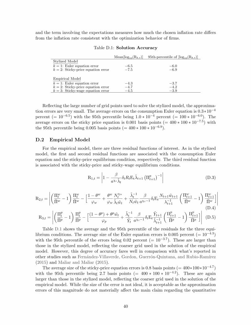
and the term involving the expectations measures how much the chosen inflation rate differsfrom the inflation rate consistent with the optimization behavior of firms.

Table D.1: Solution Accuracy

Mean[log10(Rk,t)] 95th-percentile of [log10(Rk,t)]Stylized Model

k = 1: Euler equation error −6.5 −6.0k = 2: Sticky-price equation error −7.5 −6.9

Empirical Model

k = 1: Euler equation error −4.3 −3.7k = 2: Sticky-price equation error −4.7 −4.2k = 3: Sticky-wage equation error −4.5 −3.9

Reflecting the large number of grid points used to solve the stylized model, the approxima-tion errors are very small. The average errors on the consumption Euler equation is 0.3∗10−4

percent (= 10−6.5) with the 95th percentile being 1.0 ∗ 10−4 percent (= 100 ∗ 10−6.0). Theaverage errors on the sticky price equation is 0.001 basis points (= 400 ∗ 100 ∗ 10−7.5) withthe 95th percentile being 0.005 basis points (= 400 ∗ 100 ∗ 10−6.9).

D.2 Empirical Model

For the empirical model, there are three residual functions of interest. As in the stylizedmodel, the first and second residual functions are associated with the consumption Eulerequation and the sticky-price equilibrium condition, respectively. The third residual functionis associated with the sticky-price and sticky-wage equilibrium conditions.

R1,t =

∣∣∣∣1− β

aχc λtδtRtEtλt+1

(Πpt+1

)−1∣∣∣∣ (D.3)

R2,t =

∣∣∣∣∣(

Πwt

Πw− 1

)Πwt

Πw−[1− θw

ϕw+θw

ϕw

Nχnt

λtwt+

λ−1t

Ntwt

β

aχc−1δtEt

Nt+1wt+1

λ−1t+1

(Πwt+1

Πw− 1

)Πwt+1

Πw

]∣∣∣∣∣(D.4)

R3,t =

∣∣∣∣∣(

Πpt

Πp− 1

)Πpt

Πp−[(1− θp) + θpwt

ϕp+λ−1t

Yt

β

aχc−1δtEt

Yt+1

λ−1t+1

(Πpt+1

Πp− 1

)Πpt+1

Πp

]∣∣∣∣∣ (D.5)

Table D.1 shows the average and the 95th percentile of the residuals for the three equi-librium conditions. The average size of the Euler equation errors is 0.005 percent (= 10−4.3)with the 95th percentile of the errors being 0.02 percent (= 10−3.7). These are larger thanthose in the stylized model, reflecting the coarser grid used in the solution of the empiricalmodel. However, this degree of accuracy fares well in comparison with what’s reported inother studies such as Fernandez-Villaverde, Gordon, Guerron-Quintana, and Rubio-Ramırez(2015) and Maliar and Maliar (2015).

The average size of the sticky-price equation errors is 0.8 basis points (= 400∗100∗10−4.7)with the 95th percentile being 2.7 basis points (= 400 ∗ 100 ∗ 10−4.2). These are againlarger than those in the stylized model, reflecting the coarser grid used in the solution of theempirical model. While the size of the error is not ideal, it is acceptable as the approximationerrors of this magnitude do not materially affect the main claim regarding the quantitative

40

importance of the deflationary bias. The instances of large approximation errors are onlyobserved in the area of the state space where the discount rate shock is high and the policyrate is constrained by the effective lower bound.

The sticky-wage equation errors are somewhat larger than the sticky-price equation errors.The average size is 1.3 basis points (= 400 ∗ 100 ∗ 10−4.5) with the 95th percentile being 4.9basis points (= 400 ∗ 100 ∗ 10−3.9). However, given that the standard deviation of the wageinflation is more than two times as large as that of the price inflation (66 versus 31 basispoints), the sticky-wage equation errors are smaller in relative terms than the sticky-priceequation errors. As in the sticky-price equation error, the instances of larger approximationerrors are only observed in the area of the state space where the discount rate shock is highand the policy rate is constrained by the effective lower bound.

E Expected Time Until the Liftoff

In this section, we present the survey-based measures of the expected time until the liftoffto support the claim that the market participants consistently underestimated the durationof the lower bound episode since the federal funds rate hit the lower bound in late 2008. Thesurveys we examine are (i) the Blue Chip Surveys, (ii) the Survey of Professional Forecasters,and (iii) the Primary Dealers Survey.

The evidence from all three surveys is consistent with the claim that the market partici-pants have consistently underestimated the duration of the lower bound episode. In particu-lar, for the first two years of the lower bound episode, the market participants expected thatthe federal funds rate to stay at the ELB only for additional few quarters.28

E.1 Blue Chip Surveys

The Blue Chip Surveys consists of two monthly surveys, the Blue Chip Economic Indi-cators Survey and the Blue Chip Financial Forecasts Survey. These two surveys ask theirparticipants (about 50 financial institutions for each survey) their forecast paths of variousmacroeconomic variables, including the 3-month Treasury Bill rate in the Economic Indi-cators Survey and the federal funds rate in the Financial Forecasts Survey. The near-termforecast horizon is up until the end of next calendar year and the frequency of the projectionis quarterly. Thus, the forecast path of the Treasury rate or the federal funds rate can tellus the expected time until the liftoff when the participants expect the first liftoff to occurwithin two years.

Twice a year, the surveys ask longer-run projections of certain variables in the specialquestion section (March and October for the Economic Indicators and June and Decemberfor the Financial Forecasts). The longer-run forecasts are in annual frequency for next 5 to 6years. Towards the end of the lower bound episode, the Surveys also asked the participantsto provide the expected liftoff date in the special questions section.

For each survey, we combine these various pieces of information in the following wayto construct a series for the expected period until the liftoff. First, we use the averageprobability distribution over the timing of the liftoff to compute the expected time until theliftoff whenever that information is available. Second, if the probability distribution is notavailable, we use the information from the near-term forecasts. The time of liftoff is defined

28While not shown, the expected duration of the lower bound episode based on the expected policy pathimplied by the federal funds rate futures is also consistent with this claim.

41

to be the first quarter when the median federal funds rate forecast exceeds 37.5 basis points.Finally, when the policy rate is projected to stay at the ELB until the end of the near-termforecast horizon, we use the information from the long-run projections if the Survey has thatinformation and leave the series blank when the Long-Range section is not available.

Figure E.1: Expected Time Until Liftoff†

2009 2010 2011 2012 2013 2014 2015 20160

2

4

6

8

10

12

Year

Dura

tion (

in q

uart

ers

)

Blue Chip Economic Indicators

2009 2010 2011 2012 2013 2014 2015 20160

2

4

6

8

10

12

Year

Dura

tion (

in q

uart

ers

)

Blue Chip Financial Forecasts

2009 2010 2011 2012 2013 2014 2015 20160

2

4

6

8

10

12

Year

Du

ration (

in q

uart

ers

)

Primary Dealers Survey

2009 2010 2011 2012 2013 2014 2015 20160

2

4

6

8

10

12

Year

Du

ration (

in q

uart

ers

)Survey of Professional Forecasters

† Data sourced from: Blue Chip Economic Indicators Survey (from January 2009 to August 2015); Blue Chip FinancialForecasts Survey (from January 2009 to August 2015); Federal Reserve Bank of New York, Primary Dealer Survey,accessed September 2015, https://www.newyorkfed.org/markets/primarydealer˙survey˙questions.html; Federal ReserveBoard, Survey of Professional Forecasters, accessed September 2015, https://www.philadelphiafed.org/research-and-data/real-time-center/survey-of-professional-forecasters/

The top two panels in figure E.1 show the evolutions of the expected period until liftoffbased on the Blue Chip Economic Indicators Survey and the Blue Chip Financial ForecastsSurvey. According to both panels, the market participants expected the lower bound episodeto be transitory in the early stage of the lower bound episode. The expectation shifted inthe second half of 2011, with the expectated duration of staying at the ELB exceeding 2years. Starting in late 2012 or early 2013, the survey respondents gradually reduced theirexpectation for the additional duration of the lower bound episode.

E.2 Primary Dealers Survey

The Primary Dealers Survey (the PD Survey in the remainder of the text), conducted bythe Federal Reserve Bank of New York, asks primary dealers about their policy expectationseight times a year. The survey asks its participants their probability distribution over theliftoff timing (quarter or FOMC meeting). We compute the expected time until the liftoffusing the average probability distribution over the liftoff timing. The results of the PD Survey

42

are publicly available since January 2011.The bottom-left panel of figure E.1 shows the evolution of the expected period until the

liftoff based on the PD Survey. Consistent with the measures based on the Blue Chip survey,the expected duration of the additional period of the lower bound episode increase markedlyin the second half of 2011. The expected duration hovers around 10 quarters during 2012,and has declined steadily since then.

E.3 Survey of Professional Forecasters

The Survey of Professional Forecasters (SPF) is a quarterly survey of about 40 individ-uals in academia, financial industries, and policy institutions, administered by the FederalReserve Bank of Philadelphia. Like the Blue Chip Surveys, the SPF asks its participantstheir projections of various macroeconomic variables, including the 3-month Treasury rate.For the near-term projection that extends to the end of the next calendar year, the forecastsare available in quarterly frequency. For the longer horizon, the forecast is available in annualfrequency.

The bottom-right panel of figure E.1 shows the evolution of the expected period untilliftoff based on the SPF. Consistent with the Blue Chip Surveys and the Primary DealersSurvey, the SPF shows that the market anticipated the lower bound episode to last for onlyabout one additional year until the second half of 2011. The expected duration averagesabout 9 quarters in 2012 and 2013. The expected duration started declining in the secondhalf of 2013 and has come down to 2 quarters in February 2015.

F Low inflation prior to the ELB episodes

Figure F.1 shows the evolution of inflation and policy rate past two decades in six selecteconomies (U.S., Canada, Euro Area, U.K., Sweden, and Switzerland). We exclude Japanbecause the policy rate in Japan has been at the ELB for most of the past two decades andthus the Japanese economy is better described by the deflationary equilibrium that fluctuatesaround a deflationary steady state in the context of sticky-price models.29 In all of the sixeconomies, the policy rate became constrained at the ELB during the recent global recessionfor the first time in the post WWII era and the central bank has an explicit inflation targetof 2 percent.

Figure F.2 shows the average inflation in these six economies over the period when thepolicy rate was above the ELB. Since the sample period is short, the figure shows how theconditional average depends on the starting date of the sample as well as the confidence bandfor plus/minus two standard errors.

According to the figure, inflation averaged below the inflation target while the policy ratewas away from ELB the all six countries. In the U.S. and Canada, inflation averaged about 20and 30 basis point below the 2 percent target while the ELB was not binding. The conditionalaverages in these two countries are closer to 2 percent and the confidence band includes 2percent when the starting date of the sample is around 2000. Thus, we cannot completelyrule out the possibility that the observed undershooting of the inflation target is statisticallyinsignificant. However, the figures for the U.S. and Canada demonstrate the overall tendencyfor the central banks to undershoot the long-run target by non-trivial amount in these twocountries. In the Euro Area, the United Kingdom, Sweden, and Switzerland, the conditional

29Aruoba, Cuba-Borda, and Schorfheide (2014) provide an empirical support for this view.

43

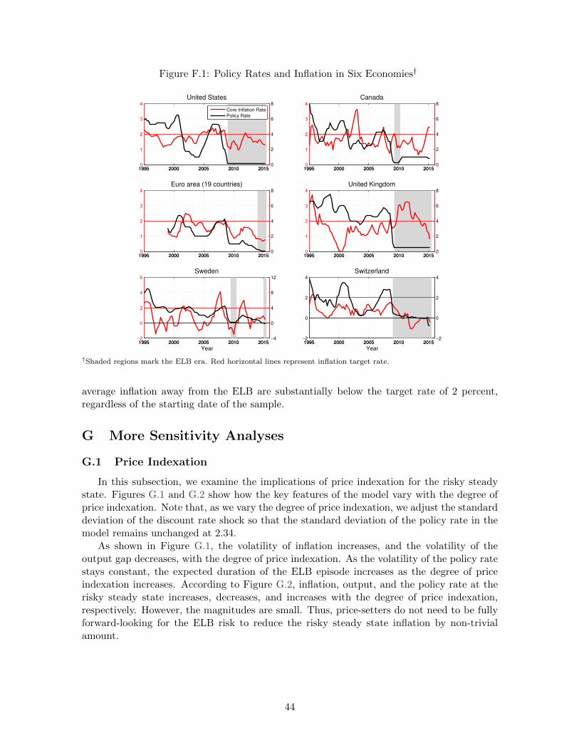
Figure F.1: Policy Rates and Inflation in Six Economies†

1995 2000 2005 2010 20150

1

2

3

4

United States

1995 2000 2005 2010 20150

2

4

6

8

Core Inflation Rate

Policy Rate

1995 2000 2005 2010 20150

1

2

3

4

Canada

1995 2000 2005 2010 20150

2

4

6

8

1995 2000 2005 2010 20150

1

2

3

4

Euro area (19 countries)

1995 2000 2005 2010 20150

2

4

6

8

1995 2000 2005 2010 20150

1

2

3

4

United Kingdom

1995 2000 2005 2010 20150

2

4

6

8

1995 2000 2005 2010 2015−2

0

2

4

6

Year

Sweden

1995 2000 2005 2010 2015−4

0

4

8

12

1995 2000 2005 2010 2015−2

0

2

4

Year

Switzerland

1995 2000 2005 2010 2015−2

0

2

4

†Shaded regions mark the ELB era. Red horizontal lines represent inflation target rate.

average inflation away from the ELB are substantially below the target rate of 2 percent,regardless of the starting date of the sample.

G More Sensitivity Analyses

G.1 Price Indexation

In this subsection, we examine the implications of price indexation for the risky steadystate. Figures G.1 and G.2 show how the key features of the model vary with the degree ofprice indexation. Note that, as we vary the degree of price indexation, we adjust the standarddeviation of the discount rate shock so that the standard deviation of the policy rate in themodel remains unchanged at 2.34.

As shown in Figure G.1, the volatility of inflation increases, and the volatility of theoutput gap decreases, with the degree of price indexation. As the volatility of the policy ratestays constant, the expected duration of the ELB episode increases as the degree of priceindexation increases. According to Figure G.2, inflation, output, and the policy rate at therisky steady state increases, decreases, and increases with the degree of price indexation,respectively. However, the magnitudes are small. Thus, price-setters do not need to be fullyforward-looking for the ELB risk to reduce the risky steady state inflation by non-trivialamount.

44

Figure F.2: Average Inflation Rates Away From the Lower Boundwith Alternative Starting Dates†

1995 1996 1997 1998 1999 2000 20011.5

1.6

1.7

1.8

1.9

2

2.1

United States

1995 1996 1997 1998 1999 2000 20011.5

1.6

1.7

1.8

1.9

2

2.1

Canada

1995 1996 1997 1998 1999 2000 20011

1.5

2

2.5

Euro area (19 countries)

1995 1996 1997 1998 1999 2000 20011

1.5

2

2.5

United Kingdom

1995 1996 1997 1998 1999 2000 20010

0.5

1

1.5

2

2.5

Start Date

Sweden

1995 1996 1997 1998 1999 2000 20010

0.5

1

1.5

2

2.5

Start Date

Switzerland

†Horizontal lines mark the inflation target rate. Dashed lines represent the 95% confidence interval (2 standard errors)of the average inflation, which is shown by the solid black lines.

Figure G.1: Moments withAlternative Degrees of Price Indexation

0 0.2 0.4 0.6 0.80.3

0.35

0.4

0.45

0.5

Price Indexation

Inflation

0 0.2 0.4 0.6 0.80.9

1

1.1

1.2

1.3

Unconditional Stdev

E[•|ELB]

0 0.2 0.4 0.6 0.82.8

2.9

3

3.1

Price Indexation

Output Gap

0 0.2 0.4 0.6 0.8−3.7

−3.5

−3.3

−3.1

0 0.2 0.4 0.6 0.82.2

2.3

2.4

Price Indexation

Policy Rate

0 0.2 0.4 0.6 0.80.12

0.13

0.14

0 0.2 0.4 0.6 0.88.8

9

9.2

9.4

9.6

Price Indexation

Quart

ers

E[ELB Duration]

45

Figure G.2: Risky Steady State withAlternative Degrees of Price Indexation

0 0.2 0.4 0.6 0.81.7

1.71

1.72

1.73

1.74

Price Indexation

RSS Inflation

0 0.2 0.4 0.6 0.80.29

0.3

0.31

0.32

0.33

0.34

Price Indexation

RSS Output Gap

0 0.2 0.4 0.6 0.83.18

3.19

3.2

3.21

3.22

3.23

3.24

3.25

Price Indexation

RSS Policy Rate

0 0.2 0.4 0.6 0.814.5

15

15.5

Price Indexation

0 0.2 0.4 0.6 0.86.4

6.7

7x 10

−3

σd

ELB Frequency

Stdev[Demand Shocks]

G.2 Wage Indexation

In this subsection, we examine the implications of wage indexation for the risky steadystate. Figures G.3 and G.4 show how the key features of the model vary with the degree ofwage indexation. Note that, as we vary the degree of wage indexation, we adjust the standarddeviation of the discount rate shock so that the standard deviation of the policy rate in themodel remains unchanged at 2.34.

As shown in Figure G.3, the volatilities of inflation, the output gap, and the policy rate aswell as the expected duration of the ELB episode increase with the degree of wage indexation.According to Figure G.2, inflation, output, and the policy rate at the risky steady statedecreases, increases, and decreases with the degree of wage indexation, respectively. Theeffects of wage indexation on the risky steady state is quantitatively large. For example,inflation is about 1.03 percentage point and the policy rate is about 2.17 percent at the riskysteady state when the degree of wage indexation is 0.4. Thus, even when wage-setters arenot fully forward-looking, the wedge between the risky and deterministic steady states canbe large.

46

Figure G.3: Moments withAlternative Degrees of Wage Indexation

0 0.1 0.2 0.3 0.40.3

0.35

0.4

0.45

0.5

Wage Indexation

Inflation

0 0.1 0.2 0.3 0.40.4

0.6

0.8

1

1.2

Unconditional Stdev

E[•|ELB]

0 0.1 0.2 0.3 0.43

3.25

3.5

3.75

4

Wage Indexation

Output Gap

0 0.1 0.2 0.3 0.4−4

−3.5

−3

−2.5

−2

0 0.1 0.2 0.3 0.42

2.2

2.4

2.6

2.8

3

Wage Indexation

Policy Rate

0 0.1 0.2 0.3 0.40

0.2

0.4

0.6

0.8

1

0 0.1 0.2 0.3 0.48

9

10

11

12

Wage Indexation

Quart

ers

E[ELB Duration]

Figure G.4: Risky Steady State withAlternative Degrees of Wage Indexation

0 0.1 0.2 0.3 0.41

1.2

1.4

1.6

1.8

2

Wage Indexation

RSS Inflation

0 0.1 0.2 0.3 0.40

0.5

1

1.5

Wage Indexation

RSS Output Gap

0 0.1 0.2 0.3 0.42

2.5

3

3.5

Wage Indexation

RSS Policy Rate

0 0.1 0.2 0.3 0.410

15

20

25

30

Wage Indexation

0 0.1 0.2 0.3 0.46

6.5

7

7.5

8x 10

−3

σd

ELB Frequency

Stdev[Discount Factor Shocks]

G.3 A Model with Monetary Policy Shocks

In this subsection, we introduce monetary policy shocks into the baseline empirical model.The standard deviation of the monetary policy shock is set to the standard deviation of theresiduals in the interest-rate feedback rule computed using the U.S. data before the federalfunds rate hit the ELB (σr = 0.14

100 ). The standard deviation of the discount rate shock isadjusted so that the standard deviation of the policy rate in the model remains unchangedat 2.34.

47

As shown in Table G.1, The moments and risky steady states of this model are similarto those of the baseline empirical model. This reflects the fact that the magnitude of themonetary policy shock is very small, accounting for only less than 5 percent of the totalvariation in the policy rate.

Table G.1: A Model with Monetary Policy Shocks

(a) Moments

Moment VariableModel Model Data

(original) (w/ MP shocks) (1995Q3–2015Q2)

St.Dev.(·)Output gap 3.0 2.9 2.9

Inflation 0.31 0.29 0.52Policy rate 2.34 2.34 2.34

E(X|ELB)Output gap −3.7 −3.3 −5.2

Inflation 1.21 1.28 1.48Policy rate 0.13 0.13 0.13

ELBFrequency 13.8% 13.5% 36%

Expected/Actual Duration 8.6 quarters 6.3 quarters 26 quarters

· 100σε,δ 0.69 0.67 ·(b) Risky Steady State†

Inflation Output Gap Policy Rate

DSS 2 0 3.75

RSS (w/ σr = 0.14100 ) 1.75 0.27 3.28

(Wedge) (−0.25) (0.27) (−0.47)

RSS (original) 1.74 0.30 3.26(Wedge) (−0.26) (0.30) (−0.49)

†DSS stands for ‘Deterministic Steady State’ while RSS stands for ‘Risky Steady State.’

G.4 A Model with TFP Shocks

In this subsection, we introduce TFP shocks into the baseline empirical model in sucha way that the standard deviations of output, inflation, and the policy rate are roughlyunchanged from the baseline empirical model. To do so, we adjust a few parameters (ϕp = 700and φπ = 3.5) and choose the size of the standard deviation of the TFP shock so that thevolatility of output explained by the TFP shock accounts for 10 percent, as opposed to 25percent, of the total output volatility. This model is used in the non-technical summary ofthis paper.

As shown in Table G.2, the moments and risky steady states of this model is broadlysimilar to those of the baseline empirical model.

48

Table G.2: A Model with TFP Shocks

(a) Moments

Moment VariableModel Model Data

(original) (w/ TFP shocks) (1995Q3–2015Q2)

St.Dev.(·)Output gap 3.0 3.1 2.9

Inflation 0.31 0.42 0.52Policy rate 2.34 2.34 2.34

E(X|ELB)Output gap −3.7 −3.4 −4.2

Inflation 1.21 1.18 1.48Policy rate 0.13 0.13 0.13

ELBFrequency 13.8% 15.9% 36%

Expected/Actual Duration 8.6 quarters 9.0 quarters 26 quarters

· 100σε,δ 0.69 0.66 ·(b) Risky Steady State†

Inflation Output Gap Policy Rate

DSS 2 0 3.75

RSS (w/ TFP shocks) 1.71 0.32 3.04(Wedge) (−0.29) (0.32) (−0.71)

RSS (original) 1.74 0.30 3.26(Wedge) (−0.26) (0.30) (−0.49)

†DSS stands for ‘Deterministic Steady State’ while RSS stands for ‘Risky Steady State.’

H Distribution of Inflation in a Perfect-Foresight Version ofthe Stylized Model

Figure H.1 shows the unconditional distribution of inflation in the perfect-foresight versionof the model. The distribution is positively skewed, reflecting the fact that the nonlinearityassociated with the ELB is dominated by the other nonlinear features of the model. Asa result, the unconditional average of inflation is slightly above 2 percent. The standarddeviation of the discount rate shock is the same as the one for the stochastic model. Withthis standard deviation, the probability of being at the ELB is x percent in the perfect-foresight model.

Figure H.2 shows how the unconditional average of inflation and the conditional averagesof inflation at and away from the ELB vary with the probability of being at the ELB in themodel with the ELB constraint solved under the assumption of perfect-foresight.

When the probability of being at the ZLB is sufficiently small, the unconditional averageof inflation is slightly positive, reflecting the positive skewness implied by other nonlinearfeatures of the model besides the ELB. However, when the probability of being at the ELBis sufficiently high, the distribution becomes negatively skewed and the average inflationbecomes below 2 percent. The conditional average of inflation away from the ELB monoton-ically increases with the probability of being at the ELB. In the perfect-foresight version ofthe model with the ELB, the median of inflation is always 2 percent. As the ELB frequencyincreases, there are more masses on the areas of the distribution where the ELB binds andthe conditional average of inflation in those areas decrease with the probability of being atthe ELB. The conditional average of inflation away from the ELB is by definition the averageinflation in the region that excludes those areas with low inflation. Thus, as the probabilityof the ELB frequency increases, the conditional average of inflation at the ELB increases.

49

Figure H.1: Unconditional Distribution of Inflationin a Perfect-Foresight Version of the Stylized Model

−6 −4 −2 0 2 4 6 8

Skewness: 0.1283

ELB Binds

Inflation Target: 2Average Inflation: 2.03

1.5 2 2.5

Figure H.2: Conditional and Unconditional Averages of Inflationin a Perfect-Foresight Version of the Stylized Model

0 2 4 6 8 10 121.9

2

2.1

2.2

2.3

2.4

2.5

Prob[Rt = 1] (in %)

Inflation (

Annualiz

ed %

)

E[Π]

E[Π|Rt > 1]

0 2 4 6 8 10 12−2

−1.8

−1.6

−1.4

−1.2

−1

−0.8

−0.6

Prob[Rt = 1] (in %)

Inflation (

Annualiz

ed %

)

E[Π|Rt = 1]

As discussed in the main text, the increase is non-monotonic in the stochastic model withthe ELB; The conditional average of inflation away from the ELB initially increases, but laterdeclines, with the ELB frequency. Unlike in the perfect-foresight version of the model, anincrease in the probability of being at the ELB shifts down the distribution of inflation, as theforward-looking price-setters take into account the ELB risk in their pricing decisions. Thisforce dominates the other force to increase the conditional average of inflation away from theELB, and lowers the conditional average of inflation away from the ELB. Provided that theELB frequency is sufficiently high, the conditional average of inflation away from the ELB isbelow 2 percent in the stochastic model where price-setters take the ELB risk into account,

50

while it is above 2 percent in the perfect-foresight version of the model that abstracts fromthe ELB risk. As a result, the fact that the conditional average fell below 2 percent whenthe policy rate is away from the ELB can be seen as the manifestation of the ELB risk, anidea that is pursued in Section 5.

51