the road to calibrating ultrasonic acoustic doppler ...the road to calibrating ultrasonic acoustic...

IGHEM-2012, June 27-30, Trondheim, Norway

1/4

The road to calibrating Ultrasonic Acoustic Doppler Current Meters

in the Swiss towing tank for hydrometric instruments

Thomas Schott

Abstract

The accredited calibration facility for hydrometric current me-ters in Ittigen, Switzerland, offers calibration services in the range from 0.02 m/s to 10 m/s for the following types of flow meters: hydrometric impellers, magneto-inductive and Acous-tic Doppler Current Meter (ultrasonic measuring instruments).

The calibration procedure of Acoustic Doppler Current Meters (ADC) is not identical to the calibration procedure for hydro-metric impellers or magneto-inductive instruments. This pre-sentation reports about the finding of a technique to be able to calibrate ADCs and gives a short description about the Cali-bration procedure.

Introduction

The Swiss calibration laboratory for hydrometric instru-ments started its work in 1896 with a tow tank of 180 m length, 1.2 m width and 1.4 m in depth (Picture above on the right).

A new tank was constructed in 1951, now with a length of 140 m but a width of 4 m and 2 m in depth. Up to 1990 only current meters had been calibrated.

In 1968 the trolley of 1951 was replaced by a new one with the current velocity range from 0.02 m/s to 10 m/s (Picture on the right).

In 1990 we started to study ways how to calibrate other instruments than impeller current meters. First we received the accreditation for magneto-inductive velocity meters.

But more popular and more often used became the Acoustic Doppler Current meters (ADC), so we wanted to be able to calibrate these instruments as well.

2/4

Finding the perfect sediment

Because the ADC use the suspended sediments in the water to detect the velocity, we had to find a way to keep small particles in suspension in the water of the tow tank, so that we can run the measuring instrument through the still water and see some reflections from the particles.

In a first test, we put some very fine sand from one of our gauging stations in the tow tank, and hoped that after stirring it up, the particles would stay long enough in suspension.

With an irrigation tube, like they are used to water the herbs in gardens, we tried to stir up the sand, by pumping air trough this tube (Pic-ture on the right).

Samuel Graf, who was the head of the calibra-tion tank from 1997 to 2008, was searching for a material that is very powdery and has the specific weight of water. He found a product from EMS Chemie called Grillamid L16. It has the specific weight of 1008 kg/m3 which is very close to water. But this powder did stick together and build clumps that settled down on the bottom.

From HSVE in Hamburg Mister Graf received the hint to use Vestosint 1111 from Degussa. This product has a specific weight of 1016kg/m3 (at 23°C) and works better be-cause it doesn’t stick together as much as the Grillamid did.

Both products are a Polyamide 12, are non-toxic and can be used in the food industry, for example for storage containers.

When a material was found that worked for the measurement, there was still the question how to mix the powder in the water, in such a way that the particles are uniformly distributed.

After the experience with the irrigation tube, we thought that the particles of our powder must be „placed“ in the water. To disperse the particles very evenly, we pumped some water from the tank in a mixer, where we mixed up the powder with the water and let it flow back somehow in the middle range of the tank. A lot of work and perhaps not necessary.

Even when Polyamide 12 doesn’t harm the environment, it’s still plastic and because man brings a lot of plastics in the biosphere, we thought it would be nice to have particles in our tow tank that are in some kind „organic“.

Our chemistry employee had the idea to use the spore of Lycopodium (Picture on the right), witch is often used for tracer measurement in the water, and we thought that it could work. So we bought a little of these spores and made tests in comparison with the Vestosint 1111.

3/4

We mixed the two products in water in two plastic tanks. With an Acoustic Doppler Current Meter we measured the dispersion and concentration of the suspended particles using the Signal to Noise ratio. We figured out that the Lycopodium stays longer in suspension than the Polyamide. So we bought 15kg of this stuff and when we changed the water in our tank we added the Lycopodium instead of the Vesto-sint.

After a few weeks, the spores of this Lycopodium were sticking on the wall of the tank and none was in suspension in the water. Now I have to mention that the tow tank is made from cement, while our test basins were made from Polyester. So here is a difference between the containers we didn’t think about.

We learned: The Lycopodium spores go in the pores of the cement while the Polyamide grains don’t.

Finding a mixing method

Again we changed the water and added our old product, the Vestosint 1111, to the water. But now we simply strew the powder in the tank when we let new water flow in. This way we used the turbulences of the water (pouring into the tank), to mix the powder up - and this worked quite well. Especially because we always stir the water up before a Doppler calibration procedure. To stir up, we use 3 special rods that we fix on the trolley and let it run a couple of times through the tank. (Picture on the right)

We do this because, we figured out, that when we calibrate over a long time only at low velocities like 1 m/s, 2 m/s, 3 m/s the particles in the water aren’t distributed evenly any more.

A question was also how many particles do we need to have a good signal response. So first there was the idea to measure the turbidity with a optical system, but then we got the pragmatic way and simply added particles to the water until we had a good signal to noise ratio (SNRdB) on the Doppler instru-ments. Typically 20 dB is a ratio where all instruments can be calibrated. Most instruments need just a little bit more than 10 dB.

Calibration procedure

While the machine can capture the pulses of current meters, measure the time and the distance auto-matically; for the ADC instruments a person has to be on the trolley and start the measurement. So this asks a little bit of experience. The person must know when the acceleration of the trolley is over, when the part of constant velocity begins and when the braking starts, so that the measuring sequence of the instrument proceeds during the part of steady velocity. Then the clocks of the Trolley and the ADC in-strument must be harmonised.

Furthermore it’s important to know how fast the measuring procedure of the instrument is, because it must have the possibility to complete a measurement but it must terminate before the braking of the trolley starts.

For example a FlowTracker of SonTek needs at least 11 seconds to finish a measuring cycle. At a speed of 2.5 m/s and a distance of 100 m of steady velocity, we have time for two measurement and 18 sec-onds for start/stop handlings, and that’s what we do.

4/4

The Calibration Laboratory for hydrometric instruments in Ittigen Switzerland is accredited according to ISO standard 17025

Since January 2011, on behalf of the Federal Office for the Environment (FOEN), the Federal Office of Metrology (METAS) is in charge of the operation of the calibration facility for hydrometric current meters:

The Federal Office of Metrology (METAS) maintains the national calibration standards of Switzerland, ensures their international recognition and disseminates them with sufficient accuracy to Switzerland's research, economy and society. METAS takes the necessary steps to ensure that the measurements required for the protection and safety of the population and the environment are made correctly and in compliance with the applicable laws and regulations.

Contact:

El.-Ing. HTL Thomas Schott

Federal Office of Metrology METAS Lindenweg 50, CH-3003 Bern-Wabern phone +41 31 324 29 33 [email protected]

www.metas.ch


1

Gravity wave effects on the calibration uncertainty of hydrometric current meters

Marc de Huu and Beat Wüthrich Federal Office of Metrology METAS, Switzerland

E-mail: [email protected]

Abstract

Hydrometric current meters are usually calibrated in tow tanks, like the calibration facility from METAS in Ittigen, Switzerland. The uncertainty budget for this installation yields a value of 0.04 % for the lowest achievable uncertainty in velocity of the towing carriage. This paper presents some results obtained from observation with Acoustic Doppler Current Meters (ADCM) on the residual currents generated from the towing of the current meters through the tank which generate surface gravity waves. Their potential impact on the calibration uncertainty is discussed and the effect of various waiting times on repeatability is shown.

1. Introduction Hydrometric current meters are used to measure the velocity distribution in open channels and are usually calibrated over a range of speeds by towing them through still water in a tow tank, following the International Standard ISO 3455 [1] for instance. Calibration of a current meter means experimental determination of the relationship between liquid velocity and either the rate of revolution of the rotating element or the velocity directly indicated by the current meter, as quoted in [1].

The uncertainty budget for the calibration facility in Ittigen, Switzerland, yields a value of 0.04 % for the velocity of the towing carriage in the range from 0.02 m/s to 10 m/s and represents the lowest achievable uncertainty assuming a perfect current meter (i.e. no contribution from the current meter) and perfectly still water. The uncertainties quoted in the calibration certificates issued by the calibration facility apply to the actual measurements of the number of revolutions per second of the impeller at a certain towing speed and can strongly vary depending on the quality of the current meter.

The successive measurements through the tank perturb the water and generate residual currents which can interfere and increase the velocity noise of the current meter or add a systematic error. To limit this noise, waiting times between successive runs are introduced to allow for the decay or the damping of these residual currents. The time needed for the water to still depends on several factors like the dimensions of the tank, the previous test velocity and the type of


2

suspension equipment immersed in the water. Damping or stilling devices can reduce the reflection of disturbances in the water by the end walls of the tank.

This paper will present results obtained from observations with Acoustic Doppler Current Meters (ADCM) on the residual currents generated from the towing of current meters through the tank and their effects on the uncertainty using mechanical hydrometric current meters. All measurements have been performed in the tow tank, which has a length L of 140 m, a width of 4 m and a depth of 2 m, of the calibration facility in Ittigen between the end of 2011 and April 2012. The water level H in the tank is around 1.7 m.

2. Water motion and surface gravity waves The assumption that water in a tow tank is perfectly still is not valid. There are always residual velocity fields from previous disturbances or other convection effects. Ref [2] quotes values of a few mm/s for typical convection velocities in an undisturbed tank and are therefore hardly an issue for mechanical current meters, which have start-up speeds of 2 cm/s at least.

Current meters are attached through rods to the towing vehicle and when dragged through the water will push on the water and generate a wake and a propagating wave. The wave motion that occurs at the free surface of the water, where gravity plays the role of the restoring force, is called a surface gravity wave and its dispersion relation (relation between frequency and wavelength) can be found in textbooks [3] and reads

� = �� tanh�� (1)

where πνω 2= is the circular frequency, g the earth’s gravitational acceleration, λπ2=k the

wavenumber, λ the wavelength and H the depth of the water. Depending on the ratio between the

wavelength λ of the wave and the depth H of the water, interesting simplifications result

�λ≪ 1�ℎ�� (2)

�λ≫ 1�� (3)

For shallow water, we can approximateλπ

λπ HH 2

)2

tanh( ≈ , which yields the following

relations for the frequency ν and the speed c of the wave

ν =

1λ�� (4)

� = ��, � = λν (5)


3

A limited body of water like a tow tank forms standing waves by reflection from the walls and a standing oscillation in such a case is called a seiche. Only certain wavelengths and frequencies are allowed by the boundary conditions from the tank and are given by

λ =

2� + 1

(6)

where L is the length of the tow tank and n denotes the mode of the wave.

A numerical application to the METAS tow tank (L = 140 m, H = 1.7 m) yields the following values:

• λ0 = 280 m for n = 0, λ1 = 140 m for n = 1, , λ2 = 93 m for n = 2

• H/λ0 = 6.1e-3 << 1, the shallow water approximation can be used

• gHc = = 4.1 m/s (with g = 10 m/s2)

• ν0 = 0.0147 Hz

• T = 1/ν0 = 67.9 s

It should be noted that in shallow water, the particle orbits due to the wave are described by ellipses with their major axis oriented along the direction of propagation of the wave. In deep water, the particle orbits are circles as can be seen in Figure 1.

Figure 1: Particle orbits of wave motion in deep, intermediate and shallow water, taken from [3].

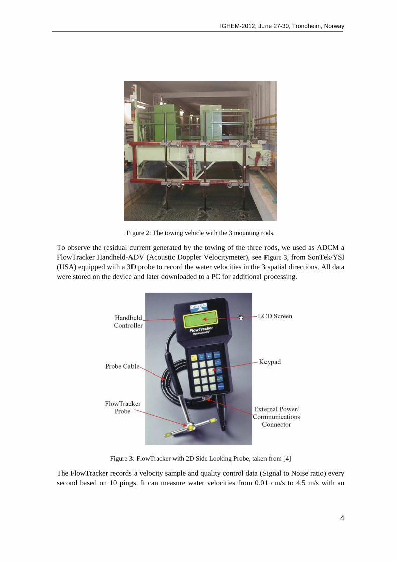
3. Water motion generation and observation method Water disturbances have been generated by towing three of our standard mounting rods of dimensions 75 mm x 35 mm through the tank, as can be seen in Figure 2 where one also recognises the seeding material in the water which is used to reflect the sound emitted by the ADCM.


4

Figure 2: The towing vehicle with the 3 mounting rods.

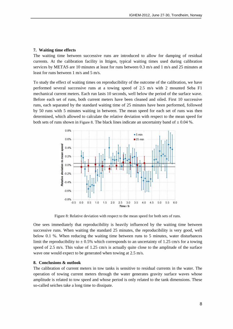
To observe the residual current generated by the towing of the three rods, we used as ADCM a FlowTracker Handheld-ADV (Acoustic Doppler Velocitymeter), see Figure 3, from SonTek/YSI (USA) equipped with a 3D probe to record the water velocities in the 3 spatial directions. All data were stored on the device and later downloaded to a PC for additional processing.

Figure 3: FlowTracker with 2D Side Looking Probe, taken from [4]

The FlowTracker records a velocity sample and quality control data (Signal to Noise ratio) every second based on 10 pings. It can measure water velocities from 0.01 cm/s to 4.5 m/s with an


5

accuracy of 1% and is especially well suited for low-flow applications [4]. The maximum recording time is limited to 1000 seconds.

Runs have been performed at towing speeds of 1 m/s, 2.5 m/s and 5 m/s. After each forward run, the towing vehicle returned to its starting position with the mounting bars retracted from the water so as to ensure maximum measurability of the wave. The standard calibration procedure from METAS asks for the mounting rods to be still immersed for the backward journey of the vehicle which occurs at a limited speed of 0.7 m/s. This situation has also been analysed and no obvious change with or without immersed rods has been observed. The FlowTracker probe was then mounted on the rod in the middle and the vehicle was moved to a position 52 m along the tank with retracted rods. At this point, the vehicle was brought to a stop and the FlowTracker probe was placed in the water at a depth of 30 cm to measure the residual water velocity. This depth corresponds to the mounting position of current meters during calibrations.

The time laps between disturbing the water, mounting and placing the FlowTracker in the water was about 3 minutes. We could only observe by eye that the generated wake decayed rapidly during this time laps.

4. Results of water motion observation The velocity of the residual current along the towing direction, after disturbing the water with a run at 1 m/s, is shown in the left part of Figure 4. The measuring time is 1000 seconds. One observes an oscillating velocity of amplitude 0.5 cm/s, consistent with the elliptical path of the particle orbits and typical for seiches, which take a long time to dissipate. The associated Fourier spectrum of this oscillation is shown in the right part of Figure 4 where one can clearly identify the 3 first modes of the surface gravity wave in excellent agreement with the numerical estimation presented in Section 2.

Figure 4: Left) Residual velocity after a run at 1 m/s. Right) Associated Fourier spectrum from the graph on the left.

Similar results have been obtained for the other towing speeds. The results for 5 m/s are shown in Figure 5.


6

Figure 5: Left) Residual velocity after a run at 5 m/s. Right) Associated Fourier spectrum from the graph on the left.

One observes the same kind of oscillations at the same frequencies. There is another visible damping, most probably due to the still present wake from the higher towing speed. The amplitude of the oscillation scales apparently with towing speed, reaching 1.2 cm/s in this case.

5. Attempt to mitigate the water motion We tried a simple and crude trick to dampen the surface wave generated by the towing rods by placing so called wave-absorbing lane lines (we called them wave-breakers) at both ends of the tow tank, like shown in Figure 6. Such devices are used in swimming pools to separate the lanes and to minimise the turbulences for the swimmers.

Figure 6: Wave-breakers mounted at both ends of the tow tank.

We spanned 3 rows of wave-breakers, on cables across the width of the tank, each separated vertically 30 cm from another, the first one being half immersed in the water. The residual velocity after disturbing the water at 1 m/s with and without wave-breakers and their associated Fourier spectra are shown in Figure 7.


7

Figure 7: Left) Residual velocity after a run at 1 m/s with and without wave-breakers. Right) Associated Fourier spectra from the graph on the left.

No clear dampening effect can be deduced from the velocity plot. The frequency spectra however indicate that the wave-breakers act like a low-pass filter and attenuate the higher order modes of the surface wave.

These results indicate that our attempt to mitigate water motion with our wave-breakers was not successful and that a more complex water-stilling device is needed. The US Hydrologic Instrumentation Facility use waste water trickling filter media placed at both ends of the tank, as well as wave-breakers placed on the side walls of the tank to attenuate the wake [5].

6. Influence on measurement uncertainty The impact of the observed surface wave on the uncertainty of the measurement has to be analysed. As can be seen in Figure 4, an oscillating velocity with amplitude 0.5 cm/s and period 67 seconds along the towing direction is still present following a run at 1 m/s after more than 15 minutes. This means that depending on when the next run starts and its duration, the current from the surface wave generate by the previous towing will be acting either along and/or against the direction of motion of the impeller during the towing and thus introducing an unknown speed contribution to the measurement.

For small towing speeds, where the current meter is towed during a time larger or similar than the oscillation period of the surface wave, the contribution from the surface wave will average over time and increase the standard deviation of the measurement. If the run lasts less than half the period of the oscillation, the contribution from the surface wave will depend on the phase relation between the start of the run and the surface wave.

At the present time, it is difficult to put hard figures on the contribution from surface waves to the measurement uncertainty because we measured the surface wave in a stationary mode while the calibration process produces a superposition between the standing surface wave and the surface wave generated by the current run. It is quite safe to say that the contribution to a 1 m/s run must be between 0 cm/s and 0.5 cm/s, depending on the phase relation between the start of the run and the surface wave. We do not have enough data at the moment. Further measurements are envisioned.


8

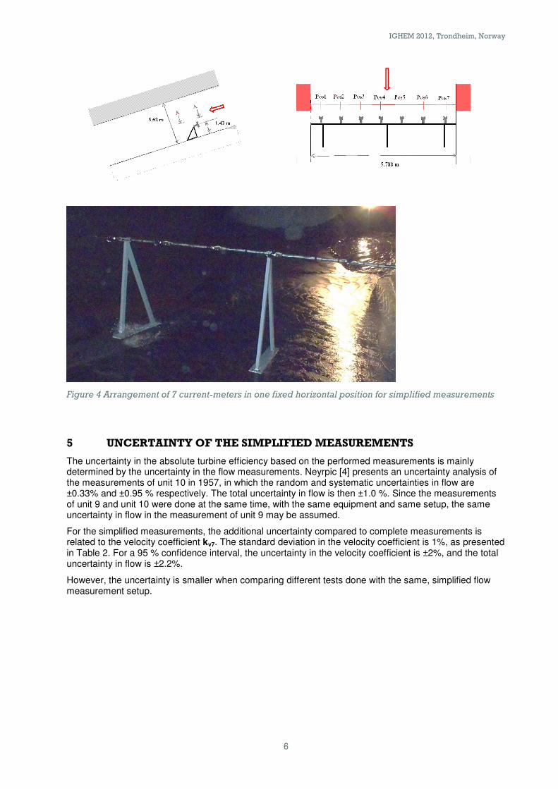
7. Waiting time effects The waiting time between successive runs are introduced to allow for damping of residual currents. At the calibration facility in Ittigen, typical waiting times used during calibration services by METAS are 10 minutes at least for runs between 0.3 m/s and 1 m/s and 25 minutes at least for runs between 1 m/s and 5 m/s.

To study the effect of waiting times on reproducibility of the outcome of the calibration, we have performed several successive runs at a towing speed of 2.5 m/s with 2 mounted Seba F1 mechanical current meters. Each run lasts 10 seconds, well below the period of the surface wave. Before each set of runs, both current meters have been cleaned and oiled. First 10 successive runs, each separated by the standard waiting time of 25 minutes have been performed, followed by 50 runs with 5 minutes waiting in between. The mean speed for each set of runs was then determined, which allowed to calculate the relative deviation with respect to the mean speed for both sets of runs shown in Figure 8. The black lines indicate an uncertainty band of ± 0.04 %.

Figure 8: Relative deviation with respect to the mean speed for both sets of runs.

One sees immediately that reproducibility is heavily influenced by the waiting time between successive runs. When waiting the standard 25 minutes, the reproducibility is very good, well below 0.1 %. When reducing the waiting time between runs to 5 minutes, water disturbances limit the reproducibility to ± 0.5% which corresponds to an uncertainty of 1.25 cm/s for a towing speed of 2.5 m/s. This value of 1.25 cm/s is actually quite close to the amplitude of the surface wave one would expect to be generated when towing at 2.5 m/s.

8. Conclusions & outlook The calibration of current meters in tow tanks is sensitive to residual currents in the water. The operation of towing current meters through the water generates gravity surface waves whose amplitude is related to tow speed and whose period is only related to the tank dimensions. These so-called seiches take a long time to dissipate.


9

The current from the surface wave introduces an unknown speed contribution to the measurement and adds a systematic uncertainty that depends on the duration of the run and the phase relation between the start of the run and the surface wave. Further measurements are needed to put numbers on the contribution from surface gravity waves.

Waiting times between successive runs allow for the water to still and their proper choices strongly influence the repeatability between measurements. An example showed that the METAS waiting times allow a good reproducibility for successive measurements.

Technical improvements to mitigate unwanted water movements in the tow tank from METAS should be introduced to further increase the accuracy of the calibration facility.

References [1] International Standard ISO 3455:2007 Hydrometry – Calibration of current meters in

straight open tanks [2] F.T. Thwaites and A.J. Williams, Use of tow tanks to study sensitive current meters,

OCEANS ’97 MTS/IEEE Conference Proceedings vol. 2 1089-1093 (1997) [3] P.K. Kundu and I.M.Cohen, Fluid mechanics 4th Edition (Academic Press, London, 2008) [4] FlowTracker Handheld ADV Technical Manual, SonTek/YSI, Inc. [5] K.G. Thibodeaux, Hydrologic Instrumentation Facility, USA, Private communication

IGHEM 2012, Trondheim, Norway

1

SIMPLIFIED CURRENT METER MEASUREMENTS USED TO VERIFY IMPROVEMENT OF TURBINE EFFICIENCY AFTER RUNNER REPLACEMENT

Erik Nilsen and Leif Parr,

Department of mechanical engineering, Norconsult AS, Norway

Jan Øystein Rafoss,

E-Co Energi AS, Norway

Petter Thorvald Krohg Østby,

Department of hydraulic design, Rainpower, Norway

SUMMARY

An 8.5 MW Francis turbine with 21 m head from 1925 has recently been equipped with a runner of new design. Complete current meter measurements were previously made in 1925 and in 1957 in the pressure conduit, with an array of 81 current meter positions. Thus, the velocity profile as a function of discharge was well known from the old report. Related to the installation of the new runner, new current meter tests have been made. It was decided to use a simplified current meter measurement, where only 7 current meters were installed on a fixed horizontal beam. The correlation between average velocity of these 7 current meters and the total discharge was found from the data in the report from the 1957 current meter measurements. Such simplified measurements were done before and after runner replacement. Even if the uncertainty in absolute efficiency is increased because of the reduced number of velocity measurements, the repeatability of the test is good. The improvement in performance of the new runner could therefore be measured with acceptable accuracy. The simplified method of measurement for verification of the guaranteed efficiency was accepted by the turbine supplier.


2

1 DESCRIPTION OF PLANT, UNITS AND HISTORY

Solbergfoss dam and power plant is located east of Oslo in Norway’s largest river, Glomma. It consists of a concrete gravity dam and two power houses with a head of about 20 m. The old power house, Solbergfoss 1, was built from 1917 to 1924, and contains 13 Francis units (12 of 8.5 MW and one of 12,5 MW) commissioned between 1924 and 1959. A new underground powerhouse, Solbergfoss 2, with one large Kaplan unit (100 MW) was commissioned in 1985.

This paper concerns unit no. 9 in the old power house. Figure 1 shows a top view of the dam and the old powerhouse. The river is lead into a forebay alongside the power house, and the discharge leaving the turbines enters a tailwater canal in the riverbed. Figure 2 shows a cross-sectional view of a unit and its water passage from intake to tailwater. About half way into the pressure conduit, guide slots for a current meter frame are arranged. All the 13 water passages are built according to the same drawing, which means that the differences are only building tolerances.

2 PREVIOUS TURBINE EFFICIENCY MEASUREMENTS

In 1997, all previous measurements at Solbergfoss I were summarized by Berdal Strømme [2]. Turbine efficiency measurements with current meters had been performed on all units during commissioning. Unit 9 was measured in 1925. Documentation of this test has not been found. The unit was measured again in 1957. This test was documented by Thoresen and Hansen [3], and contains complete tables of all flow velocities and measured values. In the same period, guarantee measurements using current meters were performed on unit 10. This test, for which the current-meter setup was identical to the test of unit 9, is reported by Neyrpic [4], and contains an evaluation of the test accuracy.

According to Thoresen and Hansen, the efficiency test of unit 9 took two days, but it is probable that the installation and deinstallation of equipment is not included. In the report of Neyrpic, the complete efficiency test of unit 10 took seven days.

3 CONDITION ASSESSMENT IN 1997

In 1997, the power company wanted to make turbine efficiency tests of the units in the old power house. The power station had so far been operated manually, but now a computerised plant control system was installed, and efficiency curves for the control system were needed. The primary goal for the measurements was to find the shape, and more specifically the peak, of the efficiency curve, in order to optimise power generation. The secondary goal was to establish an approximate absolute efficiency level. Complete current meter measurements were considered to be too expensive. Therefore, it was proposed to perform simplified current meter measurements together with Winter - Kennedy measurements on three units (no. 3, 5 and 9). As the units did not have pressure taps for Winter-Kennedy measurements, identical tap arrangements were installed in the turbine spiral cases of all of the units.

Simplified current meter measurements were made, which showed good agreement between current-meter measurements and Winter-Kennedy measurements. Therefore, Winter-Kennedy measurements were performed on the rest of the units.

The resulting efficiency curves from these measurements have since 1997 been used in the optimisation of the plant operation.


3

Figure 1 Solbergfoss I - top view. Unit 9 is marked in red. Reference: Norske kraftverker [1]

Figure 2 Cross-section of Solbergfoss I power-house. Reference: Norske kraftverker [1]

Current - meter measurement section


4

4 SIMPLIFIED CURRENT-METER SETUP

The concept of simplified current-meter measurements was concieved from an analysis of the previous current meter measurements reported by Thoresen and Nybro Hansen [3] and Neyrpic [4]. The full current meter measurements used a current meter beam with 9 current meters that were positioned in 9 levels. A total of 81 velocities were recorded to determine the turbine discharge, as seen in Figure 3. The measurements show that the velocity profile is even and symmetrical, which is due to the straight inflow conduit.

The velocity profiles at various discharges were analysed, and the 3rd

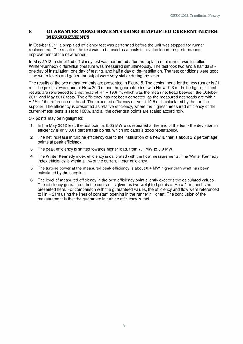
level from the bottom was selected as a reference level (marked in red in Figure 3). Table 1 shows the measured velocities in the selected level for all test points. As is shown in Table 2, the ratio between the average measured velocity of the current meters in the selected level and the flow calculated using all 81 current-meter velocities (kv9 and kv7) was almost constant. Also, it was found that not using the two current meters closest to the left and right conduit walls would not significantly affect the accuracy of the established correlation. The conclusion of these findings was that a fairly accurate discharge measurement could be made with 7 current meters installed on a fixed horizontal beam in the reference position. The simplified arrangement of the current meters is shown in Figure 4.

Table 1 Flow velocities in 3rd leel from bottom, from current-meter measurements of unit 9 in 1957 [3]

Test no. Velocity (m/s) in position number

1 2 3 4 5 6 7 8 9

I 0.960 0.950 1.009 1.061 1.001 0.990 0.992 0.948 0.848

II 1.131 1.235 1.163 1.247 1.192 1.194 1.189 1.155 0.993

III 1.256 1.290 1.302 1.388 1.297 1.296 1.309 1.209 1.103

IV 1.292 1.231 1.393 1.454 1.312 1.345 1.359 1.257 1.112

V 1.361 1.315 1.475 1.535 1.417 1.530 1.444 1.364 1.158

VI 1.340 1.372 1.533 1.555 1.462 1.483 1.491 1.427 1.216

VII 1.545 1.525 1.587 1.675 1.546 1.568 1.567 1.524 1.286

VIII 1.237 1.175 1.388 1.429 1.341 1.373 1.366 1.312 1.123

IX 1.177 1.180 1.343 1.414 1.292 1.365 1.321 1.262 1.086

Table 2 Calculated flow from current-meter measurements of unit 9 in 1956 [3], and calculated velocity

coefficients for 9 and 7 current meters respectively

9 current meters 7 current meters

Test no.

calculated flow

m

3/s

flow per area

m/s

average meas.

velocity m/s

velocity coeff. kV9 -

average meas.

velocity m/s

velocity coeff. kV7 -

I 30.55 0.953 0.973 0.979 0.993 0.959

II 36.68 1.144 1.167 0.981 1.196 0.956

III 41.00 1.279 1.272 1.005 1.299 0.985

IV 41.40 1.291 1.306 0.988 1.336 0.966

V 44.05 1.374 1.400 0.981 1.440 0.954

VI 45.75 1.427 1.431 0.997 1.475 0.967

VII 47.95 1.495 1.536 0.974 1.570 0.952

VIII 41.58 1.297 1.305 0.994 1.341 0.967

IX 40.15 1.252 1.271 0.985 1.311 0.955

Average 0.9871 0.9625

Standard deviation 0.0100 0.0102

The simplified method depends on that the velocity profile does not change between the tests. The tests in 1957 were done during winter time when the river flow typically is kept quite constant, and well below the total capacity of the power station. Thus, the velocities in the forebay were moderate. For subsequent measurements, in 1997, 2011 and 2012, similar conditions were established by regulating most of the flow through the new underground power house of Solbergfoss II.


5

Figure 3 Array of 81 positions for complete current-meter flow velocity measurements. The position used

for simplified measurements is indicated in red.


6

Figure 4 Arrangement of 7 current-meters in one fixed horizontal position for simplified measurements

5 UNCERTAINTY OF THE SIMPLIFIED MEASUREMENTS

The uncertainty in the absolute turbine efficiency based on the performed measurements is mainly determined by the uncertainty in the flow measurements. Neyrpic [4] presents an uncertainty analysis of the measurements of unit 10 in 1957, in which the random and systematic uncertainties in flow are ±0.33% and ±0.95 % respectively. The total uncertainty in flow is then ±1.0 %. Since the measurements of unit 9 and unit 10 were done at the same time, with the same equipment and same setup, the same uncertainty in flow in the measurement of unit 9 may be assumed.

For the simplified measurements, the additional uncertainty compared to complete measurements is related to the velocity coefficient kv7. The standard deviation in the velocity coefficient is 1%, as presented in Table 2. For a 95 % confidence interval, the uncertainty in the velocity coefficient is ±2%, and the total uncertainty in flow is ±2.2%.

However, the uncertainty is smaller when comparing different tests done with the same, simplified flow measurement setup.


7

6 PROCESS LEADING TO A CONTRACT ON RUNNER RENEWAL

The units are mechanically robust, and had little sign of wear. Therefore, it was the relatively poor hydraulic performance found in 1997 which was the main driver for investigating the benefits of a replacement runner with a modern design. It was found that an improvement of efficiency, and an increase in the maximum power output within the 10 MVA limit of the generator together would make a replacement runner profitable.

In addition, the Norwegian government has introduced a system of economic stimulation to power companies to increase the generation of renewable energy - either by upgrading existing facilities or by building new units. The system of economic benefits, which is labelled green certificates, was not an important issue for the replacement runner project, but will become a bonus on top of existing revenues. The green certificates were introduced in 2012 - the application for certificates for unit 9 is being written, but has not at the time of publication of this paper been sent or approved.

It was decided to replace the runners in three units, replacing one runner each year starting in 2011/2012. Unit 9 was to have the first replacement runner. A request for quotation on new runner was sent out, and the Norwegian turbine manufacturer Rainpower was awarded the contract. The contract of the two subsequent runners could be altered or cancelled based on the performance of the first runner. As a basis for the performance guarantees, Rainpower was informed of the results of the simplified turbine efficiency measurements in 1997. It was agreed between E-Co and Rainpower that simplified current-meter measurements would be used to validate the efficiency guarantees of the new runners, even though the method does not comply to IEC 60041 [5]. The main deviation from the standard is the number of measurement points - the standard requires more than 25 velocity measurement points.

7 NEW RUNNER DESIGN

Designing a new runner for the existing turbine at Solbergfoss I provided several challenges. The power plant has low head and high discharge, and is better suited for a Kaplan turbine than a Francis turbine. The turbines have a specific speed, nqrpm, above 100. The new runner was to increase the existing power output by more than 20%, and operate within a large head variation (Hmax/Hmin=2) without cavitation and with good stability behaviour. In addition, the run-away speed of the new runner was limited by the generator, and the runner had to fit into the existing turbine casing without any modifications to the surrounding parts.

Normally, the starting point when designing a new runner is a well documented and similar reference model turbine which can be used for validation and comparison. During the last few years, Rainpower has developed a new generation of medium/low head Francis turbines called Rainpower Storm. Several model turbines have been developed and tested. However, none of these models have specific speeds which are in the range of Solbergfoss I. It was therefore necessary to design the new runner relying mainly on CFD results.

The design process took about two months. More than 50 different runner designs were made and tested with CFD, before the final design was ready for production. The hub, band and blades, which were made of carbon steel, were produced in China, and were welded together and painted at Rainpower’s workshop at Sørumsand, Norway.

The new runner has a design which differs significantly from the old runner. Most noticeably is the increased thickness at the inlet of the vanes which increase the performance at low heads and ensures a cavitation-free inlet. The inlet edge has also been skewed to provide a better pressure distribution at the runner inlet. Secondly, the number of blades has been reduced from 14 to 13 to reduce friction losses. Several other design choices have also been made to ensure the performance of the new runner.


8

8 GUARANTEE MEASUREMENTS USING SIMPLIFIED CURRENT-METER

MEASUREMENTS

In October 2011 a simplified efficiency test was performed before the unit was stopped for runner replacement. The result of the test was to be used as a basis for evaluation of the performance improvement of the new runner.

In May 2012, a simplified efficiency test was performed after the replacement runner was installed. Winter-Kennedy differential pressure was measured simultaneously. The test took two and a half days - one day of installation, one day of testing, and half a day of de-installation. The test conditions were good - the water levels and generator output were very stable during the tests.

The results of the two measurements are presented in Figure 5. The design head for the new runner is 21 m. The pre-test was done at Hn = 20.0 m and the guarantee test with Hn = 19.3 m. In the figure, all test results are referenced to a net head of Hn = 19.6 m, which was the mean net head between the October 2011 and May 2012 tests. The efficiency has not been corrected, as the measured net heads are within ± 2% of the reference net head. The expected efficiency curve at 19.6 m is calculated by the turbine supplier. The efficiency is presented as relative efficiency, where the highest measured efficiency of the current-meter tests is set to 100%, and all the other test points are scaled accordingly.

Six points may be highlighted:

1. In the May 2012 test, the test point at 8.65 MW was repeated at the end of the test - the deviation in efficiency is only 0.01 percentage points, which indicates a good repeatability.

2. The net increase in turbine efficiency due to the installation of a new runner is about 3.2 percentage points at peak efficiency.

3. The peak efficiency is shifted towards higher load, from 7.1 MW to 8.9 MW.

4. The Winter Kennedy index efficiency is calibrated with the flow measurements. The Winter Kennedy index efficiency is within ± 1% of the current-meter efficiency.

5. The turbine power at the measured peak efficiency is about 0.4 MW higher than what has been calculated by the supplier.

6. The level of measured efficiency in the best efficiency point slightly exceeds the calculated values. The efficiency guaranteed in the contract is given as two weighted points at Hn = 21m, and is not presented here. For comparison with the guaranteed values, the efficiency and flow were referenced to Hn = 21m using the lines of constant opening in the runner hill chart. The conclusion of the measurement is that the guarantee in turbine efficiency is met.


9

Figure 5 Results of simplified current-meter tests of unit 9 at Solbergfoss I. The efficiency is given as

index efficiency, where the highest measured efficiency of the current-meter tests is set to 100%.

9 CONCLUSIONS

The simplified current meter measurements have been successful. The uncertainty in discharge of these simplified measurements is ±2.2%, based on an analysis of complete measurements in the same measurement section. The absolute accuracy is reduced compared to complete measurements, but the repeatability between the tests of the same setup is significantly better than ±2.2%.

The turbine supplier accepted the simplified measurements for verification of turbine efficiency of the new runner.

Installation of a new runner has increased the peak efficiency by 3.2 percentage points, and has increased the maximum power output 18% at Hn = 19.6 m head.

For the power company, the important operating range is between the efficiency peak and maximum output. The measured peak efficiency was closer to the maximum output than what was specified in the contract, but this has actually proved to be beneficial to the power company, given that there are a total of 14 units in the the Solbergfoss power stations in which to optimally distribute the load.


10

10 REFERENCES

[1] Solem, A, Heggstad, R and Raabe, N, 1954, "Norske kraftverker", Teknisk ukeblads forlag.

[2] Berdal Strømme (presently Norconsult), 1997, "Mørkfoss - Solbergfossanleggene. Solbergfoss I kraftverk. Oversikt over tidligere last- og virkningsgradsmålinger."

[3] Thoresen, H and Nybro Hansen, J (presently Norconsult), 1958, "Mørkfoss - Solbergfossanlegget. Redegjørelse for hvad det er passert med de 9 første turbiner fra igangsettingen til gjennemføringen av kraftprøver og virkningsgradsprøve i januar 1957."

[4] EB, JCf / RGL, 1957, "Oslo lysverker - vassdragsvesenet. Centrale de Solbergfossen. 1 Turbine francis rapide. 17000 CV./21m. à 125 t/min. Rapport relatif aux essais de rendements de la turbine.", ETE 205 Neyrpic Grenoble.

[5] IEC, 1991-11, "Field acceptance tests to determine the hydraulic performance of hydraulic turbines, storage pumps and pump-turbines.", IEC 60041:1991(E)

Statistic evaluation of deviation between guaranteed and measured

turbine efficiency

Petr ŠevčíkHydro Power Group Leading Engineer

OSC, a.s.Czech Republic

1. Introduction

Gibson method allows to measure discharge cost effectively and with sufficient accuracy. This method is generally accepted in form described by standard [1], where straight measuring section with constant cross-section area is required. Such field tests conditions are however seldom available. Standard [2] allows use also curved penstock with parts of different cross-section areas. Nevertheless influence of all secondary interferences is discussed during preparatory works on the new standard prepared for site acceptance tests.

Large set of Gibson measurements tests results provided on HPP with variety of different penstock dimensions and shapes is available by OSC company. Due to customer usual requirement to reduce costs for acceptance test there are only a few cases for direct comparison between Gibson method and other flow measurement methods used for turbine efficiency evaluation in real plant conditions. But recently the CFD methods and preciseturbines production enable to predict and guarantee very exactly the turbine prototype parameters. Idea of this paper is contribute to the discussion regarding influence of penstock irregularities on Gibson method results.Statistic evaluation of deviation between measured prototype efficiency and guaranteed value for sample of 47 Gibson guarantee measurements was processed. Similar sample of acceptance tests results using current meters was evaluated as a comparable data too.

2. Gibson method application

Gibson flow measurement method used by OSC can be briefly described as follows:

separate pressure records are used

almost the whole penstock length is used as measuring section

the pressure sensors used are installed in exactly defined cross sections G1 and G2

measurement with free water upper level is used only when necessary (not for guarantee measurement)

calculation principles according to standard IEC 41/1991 are used

measurement may be applied on various penstock’s layouts (straight, curved, sections with different diameters, etc.)

there are no corrections for curved penstock applied

turbine unit was always stopped by emergency shut down or by similar procedure

leakage through guide vane is evaluated by Gibson method for intake valve closing or by other exact method (e.g. level drop behind stop log)

combination of Gibson and index flow measurement is always used

3. Statistic evaluation of Gibson guarantee tests

Set of guarantee measurements provided and used for statistic evaluation is summarized in Tab. 1.

Deviation between measured efficiency and guaranteed efficiency value for each plant unit was evaluated according to following formula:

M

GM

Where M = measured efficiency

G = guaranteed efficiency

Various kinds of guarantees relevant to each particular contract (weighted, average efficiency or only one guaranteed point) were used for mentioned equation. Measured efficiency value was than evaluated in accordance with those individual rules.

No. Year HPP unit Country Penstock

1 1999 PSHP Dalešice - pump turbine TG3 - GM before refurbishment - T CZ straight, L ~ 30D

2 1999 PSHP Dalešice - pump turbine TG3 - GM after refurbishment - P CZ

3 1999 PSHP Dalešice - pump turbine TG3 - GM after refurbishment - T CZstraight, L ~ 30D

4 2000 PSHP Dalešice - pump turbine TG1 before upgrade T, GM CZ straight, L ~ 30D

5 2001 PSHP Dalešice - pump turbine TG1 after upgrade, GM - T CZ

6 2002 PSHP Dalešice - pump turbine TG1 after upgrade, GM - P CZstraight, L ~ 30D

7 2002 HPP Vranov - Francis turbine after upgrade CZ curved, L ~ 15D

8 2004 PSHP Dalešice - pump turbine TG4 after upgrade - GM - T CZ

9 2004 PSHP Dalešice - pump turbine TG4 after upgrade - GM - P CZstraight, L ~ 30D

10 2005 HPP Vydra, Francis turbine TG1 after upgrade - GM CZ

11 2006 HPP Vydra, Francis turbine TG2 after upgrade - GM CZnearly straight, 930D

12 2006 HPP Les Království, Francis turbine - GM CZ straight, L ~ 15D

13 2006 HPP Kalimanci, Francis turbine TG1 - GM MK

14 2006 HPP Kalimanci, Francis turbine TG2 - GM MKstraight, L ~ 30D

15 2006 HPP Orava, Kaplan Turbine - GM SK straight, L ~ 6.7D

16 2007 HPP Pena, Francis turbine TG2 - GM MK

17 2007 HPP Pena, Francis turbine TG1 - GM MKstraight, L ~ 63D

18 2008 HPP Patikari, Pelton turbine TG1 - GM IND

19 2008 HPP Patikari, Pelton turbine TG2 - GM INDcurved, L ~ 500D

20 2008 HPP Sapunčica, Pelton turbine TG1 - GM MK

21 2008 HPP Sapunčica, Pelton turbine TG2 - GM MK

nearly straight L = 1730 m ~ 3150D

22 2008 HPP Pesocani, Pelton turbine TG1 - GM MK

23 2008 HPP Pesocani, Pelton turbine TG2 - GM MK

nearly straight L ~ 1300D

24 2008 HPP Concepción, Francis turbine TG1 - GM PA

25 2008 HPP Concepción, Francis turbine TG2 - GM PA

CurvedL ~ 50D

26 2008 HPP Matka, Kaplan turbine TG2 - GM MK

27 2008 HPP Matka, Kaplan turbine TG1 - GM MK

2x curvedL ~ 15 / 14 D

28 2008 PSHP Dalešice - pump turbine TG2 after upgrade - GM T CZ

29 2008 PSHP Dalešice - pump turbine TG2 after upgrade - GM P CZstraight, L ~ 30D

30 2009 HPP Došnica, Pelton turbine TG1 - GM MK



curved, L ~ 380D

33 2010 HPP Soběnov, Francis turbine TG1 - GM after upgrade CZ

34 2010 HPP Soběnov, Francis turbine TG2 - GM after upgrade CZcurved, L ~ 101D

35 2010 HPP Ampelgading, Francis turbine TG1 - GM RI

36 2010 HPP Ampelgading, Francis turbine TG2 - GM RIL ~ 490 D

37 2010 HPP Penz, Zeltweg, Kaplan turbine TG1 - GM A

38 2010 HPP Penz, Zeltweg, Kaplan turbine TG2 - GM A

L = 2845 mL ~ 1224 D

39 2010 HPP Rendelstein, Bolzano - 1 Kaplan Turbine - GM I L ~ 105 D

40 2010 HPP Meziboří, Francis turbines TG1, GM after refurbishment CZ

41 2010 HPP Meziboří, Francis turbines TG2, GM after refurbishment CZcurved, L ~ 1600 D

42 2011 HPP Vír II, 1 Kaplan turbine - GM CZ straight, L ~ 12D

43 2011 HPP Colmeda, Pelton turbine TG1 - GM I

44 2011 HPP Colmeda, Pelton turbine TG2 - GM Icurved, L ~ 2040 D

45 2011 HPP Seč, Francis turbine, GM after refurbishment CZ curved, L ~ 27D

46 2011 HPP Slapy TG3, GM after upgrade CZ curved, L ~ 8D

47 2012 SHPP Agia Barabara, S turbine, GM GR curved, L ~ 15D

T = turbine mode, P = pump mode of operation

Tab. 1 - List of Gibson guarantee measurements

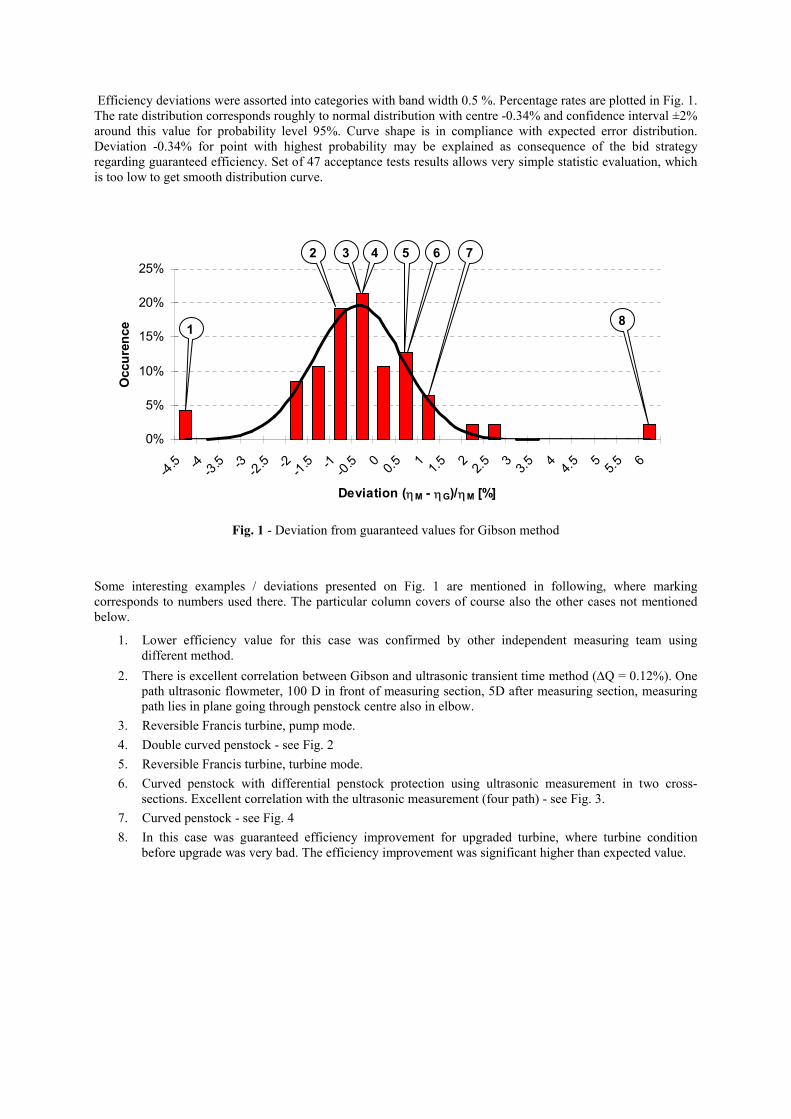
Efficiency deviations were assorted into categories with band width 0.5 %. Percentage rates are plotted in Fig. 1. The rate distribution corresponds roughly to normal distribution with centre -0.34% and confidence interval ±2% around this value for probability level 95%. Curve shape is in compliance with expected error distribution. Deviation -0.34% for point with highest probability may be explained as consequence of the bid strategyregarding guaranteed efficiency. Set of 47 acceptance tests results allows very simple statistic evaluation, whichis too low to get smooth distribution curve.

0%

5%

10%

15%

20%

25%

-4.5 -4

-3.5 -3

-2.5 -2

-1.5 -1

-0.5 0

0.5 1

1.5 2

2.5 3

3.5 4

4.5 5

5.5 6

Deviation (M - G)/M [%]

Occu

ren

ce 1

2 3 5 6

8

4 7

Fig. 1 - Deviation from guaranteed values for Gibson method

Some interesting examples / deviations presented on Fig. 1 are mentioned in following, where marking corresponds to numbers used there. The particular column covers of course also the other cases not mentioned below.

1. Lower efficiency value for this case was confirmed by other independent measuring team usingdifferent method.

2. There is excellent correlation between Gibson and ultrasonic transient time method (Q = 0.12%). One path ultrasonic flowmeter, 100 D in front of measuring section, 5D after measuring section, measuring path lies in plane going through penstock centre also in elbow.

3. Reversible Francis turbine, pump mode.

4. Double curved penstock - see Fig. 2

5. Reversible Francis turbine, turbine mode.

6. Curved penstock with differential penstock protection using ultrasonic measurement in two cross-sections. Excellent correlation with the ultrasonic measurement (four path) - see Fig. 3.

7. Curved penstock - see Fig. 4

8. In this case was guaranteed efficiency improvement for upgraded turbine, where turbine conditionbefore upgrade was very bad. The efficiency improvement was significant higher than expected value.

Fig. 2 - Double curved penstock - example 3

y = 0.99915x

R2 = 0.99980

y = 0.9961x - 0.1389

R2 = 0.9998

0

2

4

6

8

10

12

14

0 2 4 6 8 10 12 14

QG [m3/s]

QU

S [

m3/s

]

Qus1 - four paths, beginning of penstock

Qus2 - one path, end of penstock

Fig. 3 - Correlation between Gibson flow measurement and ultrasonic flow meters - example 6

Fig. 4 - Single curved penstock - example 4

Profile G1

Profile G2

Profile G1

Profile G2

4. Flow measured by current meters

Set of acceptance tests results with flow measurement using current meters (propellers) was also evaluated in similar way like discharges obtained by Gibson method. List of these measurements is presented in Tab. 2. Percentage rates are presented in Fig. 5.

No. Year HPP unit Intake Country

1 1995 HPP Slapy, Kaplan turbine - GM after reconstruction Penstock CZ

2 1996 PSHP Dlouhé stráně - pump turbine TG1, T - GM Penstock CZ

3 1996 PSHP Dlouhé stráně - pump turbine TG1, P - GM Penstock CZ

4 1996 HPP Obříství - Kaplan PIT turbine 1 - GM Low head CZ

5 1996 HPP Obříství - Kaplan PIT turbine 2 - GM Low head CZ

6 1996 HPP Veletov - Kaplan PIT turbine 1 - GM Low head CZ

7 1996 HPP Veletov - Kaplan PIT turbine 2 - GM Low head CZ

8 1997 PSHP Štěchovice - pump turbine T - GM Penstock CZ

9 1997 PSHP Štěchovice - pump turbine P - GM Penstock CZ

10 1998 HPP Libčice - Kaplan PIT turbine 1 - GM Low head CZ

11 1998 HPP Libčice - Kaplan PIT turbine 2 - GM Low head CZ

12 2000 HPP Žagań - Kaplan turbine 1 - GM Low head PL

13 2000 HPP Žagań - Kaplan turbine 2 - GM Low head PL

14 2000 HPP Žagań - Propeler turbine 3 - GM Low head PL

15 2001 HPP Ladce - Kaplan turbine after upgrade - GM Low head SK

16 2004 HPP Kisköre, Bulbturbine TG1 after upgrade - GM Low head H


18 2005 HPP Přelouč TG2, Kaplan turbine - GM Low head CZ



21 2006 HPP Vraňany, PIT turbine Low head CZ

22 2007 HPP Kroměříž, Kaplan turbine TG3 after upgrade Low head CZ

23 2008 HPP Kroměříž, Kaplan turbine TG1 after upgrade Low head CZ

24 2008 HPP Kostomlatky, Kaplan turbine TG2 after refurbishment Low head CZ

25 2009 HPP Kostomlatky, Kaplan turbine TG1 after refurbishment Low head CZ

26 2008 HPP Hradištko, Kaplan turbine TG1 after refurbishment Low head CZ

27 2008 HPP Hradištko, Kaplan turbine TG2 after refurbishment Low head CZ

28 2008 HPP Tiszalök, Kaplan turbine TG1 - after upgrade Low head H

29 2009 SHPP Lakatnik, 1 Kaplan turbine - GM Low head BG

30 2009 SHPP Svrajen, 1 Kaplan turbine - GM Low head BG

31 2009 HPP Tiszalök, Kaplan turbine - after upgrade Low head H

32 2009 SHPP Spytihněv, 2 Kaplan turbines Low head CZ

33 2010 SHPP Troja - Kaplan turbine TG1- GM Low head CZ

34 2010 HPP Tiszalök, Kaplan turbine - after upgrade Low head H

35 2011 SHHP Miřejovice - Kaplan turbine TG1 GM Low head CZ

36 2011 SHHP Miřejovice - Kaplan turbine TG2 GM Low head CZ

37 2012 SHPP Dobrohošť - 1 Kaplan turbine Low head SK

38 2012 SHPP Pardubice - 1 Kaplan turbine Low head CZ

Tab. 2 - List of propeller guarantee measurements

The rate distribution corresponds very approximately with normal distribution with centre +1.25% and confidence interval ±3%. Efficiency value obtained by flow measurement with current meters has higher dispersion of deviation from guaranteed values in comparison with Gibson method. One of the possible reasons is the fact, that approx. since 1997 no propeller flow measurement in penstock has been carried out. Current meters are applied recently only for low head power plants with rectangular intake to concrete semi spiral.Measurements with current meters installed on 6- or 8-beam spider in penstock are marked in Fig. 5. These results are closer to zero deviation in comparison with low head plants. Calculation procedure in accordance with standard [5] was used for all these tests.

0%

5%

10%

15%

20%

25%

-6-5

.5 -5-4

.5 -4-3

.5 -3-2

.5 -2-1

.5 -1-0

.5 00.

5 11.

5 22.

5 33.

5 44.

5 55.

5 6

deviation (M - G)/M [%]

Occu

rren

ce

Current meters on spider in penstock

Fig. 5 - Deviation from guaranteed values for current meters

5. Summary

The comparison of statistic evaluation between both mentioned flow measurement methods used for waterturbine efficiency evaluation is presented in Fig. 6. Reliability of Gibson method application in this case is better than method using propellers. For more serious conclusion from this comparison is necessary take in mind thatthe particular flow measurement methods weren’t used under identical conditions. Current meters flow measurements were usually carried out at low head power plants and also at the units following rehabilitation. Therefore it is not fully comparable with Gibson method, which was used for measurement under better conditions.

0%

5%

10%

15%

20%

25%

-6-5

.5 -5-4

.5 -4-3

.5 -3-2

.5 -2-1

.5 -1-0

.5 00.

5 11.

5 22.

5 33.

5 44.

5 55.

5 6

Deviation (M - G)/M [%]

Occu

rren

ce

Gibson

Current meters

Fig. 6 - Comparison between deviation distributions for Gibson method and current meters.

Percentage occurrence of deviation between measured and guaranteed efficiency values for Gibson methodcorresponds with expected normal statistic distribution. Following conclusion can be derived from this deviation distribution:

Average deviation of measured efficiency from guaranteed efficiency value -0.34% corresponds very well with expected commercial efficiency increase often used for the bid.

Deviation dispersion is done by measurement uncertainty and also by real deviation of measured efficiency against guaranteed one.

Hydraulic design based on CFD method recently used is associated with improved reliability of guaranteed parameters.

Influence of penstock layout (bends, cones etc.) on measured discharge accuracy wasn’t confirmed.

Outliers in dispersion graph (Fig. 1) were checked and fully explained.

Very good reliability of Gibson flow measurement was confirmed as well as it’s independency on penstock geometry. No any significant abnormality during all mentioned tests was noticed.

References

[1] Standard IEC 41: „Field acceptance tests to determine the hydraulic performance of hydraulic turbines, storage pumps and pump turbines“, standard issued by CEI, 1991.

[2] Standard IEC 62006, Ed. 1.0: “Hydraulic machines – Acceptance tests of small hydroelectric installations”, approved committee draft, CEI, 2007.

[3] Adamkowski A., Krzemianowski Z., Janicki W.: “Improved Discharge Measurement Using the Pressure-Time Method in a Hydropower Plant Curved Penstock”, Journal of Engineering for Gas Turbines and Power, September 2009

[4] Jonson P., Ramdal J., Cervantes M., Dahlhaug O., Nielsen T.:”The pressure-time measurement project at LTU and NTNU”, Paper for IGHEM-2010, Roorkee, India.

[5] Standard ISO 3354 “Measurement of clean water flow in closed conduits -- Velocity-area method using current-meters in full conduits and under regular flow conditions”, Czech edition, issued by ČNI 1993.

Mr. Petr Ševčík, graduated at Brno University of Technology in 1980 at Faculty of Electrical Engineering and Communication, branch Technical cybernetics. From September 1980 he worked for ORGREZ company (part of ČEZ - Czech Power Company), department of Water Power as member of site tests group. From year 1993 to 2003 he was co-owner of TS HYDRO company - services for Water Power (site acceptance tests, optimization, tests of friction losses etc.). Since year 2003 is employ os OSC company in position as Hydro Power Group Leading Engineer. He is member of the Czech national committee IEC, TC 48 – Water Turbines and member of International Group for Hydraulic Efficiency Measurement.

the road to calibrating ultrasonic acoustic doppler ...the road to calibrating ultrasonic acoustic...

Documents