GSA Data Repository 2018022

The role of asthenospheric flow during rift propagation and breakup

Luke S. Mondy1, Patrice F. Rey

1, Guillaume Duclaux

2, Louis Moresi

3

Contents

Supplemental Methods

Supplemental Figures and Tables:

Figure DR1. Temporal evolution of topography and crustal thinning along the rift of

the rotational experiment.

Figure DR2. Stress regime changes throughout the lithosphere.

Figure DR3. Mapping the evolution of gravitational potential energy (GPE) during

rotational rifting

Figure DR4. Sensitivity analyses testing the role of resolution, boundary conditions,

and partial melt.

Figure DR5. Consequences of mapping a spherical velocity field onto a Cartesian

domain.

Figure DR6. 3D view through time of the elevation of the lithosphere-asthenosphere

boundary (LAB) in both experiments.

Table DR1. Rheological parameters used.

Code and Experiment Inputs.

References

SUPPLEMENTAL METHODS

We solve the problem of conservation of mass, momentum and energy for incompressible

mantle flow and lithosphere deformation, using Underworld - an open source particle-in-cell

finite-element code (freely available at underworldcode.org), in conjunction with the

Lithospheric Modelling Recipe

(https://github.com/OlympusMonds/lithospheric_modelling_recipe), an open-source python

wrapper developed within the EarthByte group to quickly and easily setup and run

Underworld models in both 2D and 3D.

We assume a visco-plastic rheology depending on temperature, stress, strain, strain rate, and

in some experiments melt fraction (see Table DR1). The densities of all rocks depend on

temperature (see Table DR1).

Experimental setup

The experiments are run within a Cartesian box of 500 km (x-axis) by 1000 km (y-axis) and

180 km vertically (z-axis). The computational grid dimensions for solving the visco-plastic

Stokes problem is 254×512×96 (~2 km cells). A 20 km wide and 8 km deep wedge of lower

crust runs along the entire length of the experiment, to preferentially localise deformation in

the centre of the domain (Van Wijk and Blackman, 2005). A free-slip boundary condition is

imposed to the front and back walls, while a constant pressure is maintained at the bottom of

the experiment to simulate the conditions of isostatic equilibrium. The topographic surface,

which stands at sea level before rifting, evolves freely beneath a 20 km thick “sticky-air”

layer (Crameri et. al., 2012). An initial random plastic strain (up to 5%) is imposed the upper

crust to promote strain localisation near the surface.

Fundamental equations

Underworld solves the incompressible equations of continuity for momentum, energy, and

mass as below:

𝜕𝜏𝑖𝑗

𝜕𝑥𝑗−

𝜕𝜌

𝜕𝑥𝑖= −𝜌𝑔𝜆𝑖

𝜕𝑇

𝜕𝑡+ 𝑢𝑖

𝜕𝑇

𝜕𝑥𝑖=

𝜕

𝜕𝑥𝑖(𝜅

𝜕𝑇

𝜕𝑥𝑖) + 𝑄

∂𝑢𝑖

∂𝑥𝑖= 0

Where 𝑥𝑖 are the spatial coordinates, 𝑢𝑖 is the velocity, 𝑇 is temperature, 𝜌 is density, g is

gravity, 𝜆𝑖 is the unit vector in the direction of gravity, t is time, 𝜅 is thermal diffusivity, and

Q is a source term for the energy equation. Summation on repeated indices is assumed.

Additional terms can be incorporated into the above equations. In the experiments presented,

only radiogenic heating is added, unless explicitly mentioned otherwise - however, an

additional experiment was run with partial melting, and so the associated terms and values

are described below.

Both radiogenic heating and the thermal aspects of partial melting are incorporated into the

energy equations as:

𝑄radiogenic = 𝐴

𝜌𝐶𝑝

𝑄partial melt = −1 ×𝐿𝑓

𝐶𝑝

𝛿𝑀𝑓

𝛿𝑡

Where A is the rate of radiogenic heat production, 𝐶𝑝is heat capacity, 𝐿𝑓 is latent heat of

fusion, and 𝑀𝑓is the melt fraction.

The density of a material is defined via a function that depends on temperature and the melt

fraction:

𝜌 = 𝜌𝑟 × (1 − 𝛼(𝑇 − 𝑇𝑟) − (𝑀𝑓 × 𝑀𝛥𝜌𝑟))

Where 𝜌𝑟is reference density, 𝛼is thermal expansivity, 𝑇𝑟is reference temperature, and 𝑀𝛥𝜌𝑟is

the fraction of density change when melted.

The melt fraction is calculated dynamically as part of the experiment, by using the super-

solidus formula given by McKenzie and Bickle (1988):

𝑆𝑆 =(𝑇 − 𝑇𝑠)

(𝑇𝑙 − 𝑇𝑠)− 0.5

𝑀𝑓 = 0.5 + 𝑆𝑆 + (𝑆𝑆2 − 0.25) × (0.4256 + 2.988 × 𝑆𝑆)

Where SS is the normalised super-solidus temperature, Ts is the solidus, and Tl is the liquidus.

The solidus and liquidus are defined as:

𝑇𝑠 = 𝑡1 + 𝑡2𝑃 + 𝑡3𝑃2

Where P is pressure, t1, t2, and t3 are defined Table DR1.

The constitutive behaviour is assumed to be visco-plastic rheologies. For the viscous

component, flow is computed using dislocation creep (Hirth and Kohlstedt, 2003):

휀disc = 𝐴𝜎𝑛𝑑−𝑝𝑓𝐻2O𝑟 exp (−

𝐸 + 𝑃𝑉

𝑛𝑅𝑇)

Where 휀 is the effective strain-rate, A is the pre-exponential factor, n is the stress exponent, d

is the grain-size, p is the grain-size exponent, fH2O is the water fugacity, r is the water fugacity

exponent, E is the activation energy, P is the pressure, V is the activation volume, R is the gas

constant, and T is the temperature.

For the plastic component, failure is determined using the Drucker-Prager model:

√𝐽2 = 𝐴𝑝 + 𝐵

Where √𝐽2 is the second invariant of the deviatoric stress tensor, p is the pressure, and A and

B are defined as:

𝐴 =2𝑠𝑖𝑛𝜙

√3(3 − 𝑠𝑖𝑛𝜙)

𝐵 =6𝐶𝑐𝑜𝑠𝜙

√3(3 − 𝑠𝑖𝑛𝜙)

Where C is the cohesion, and 𝜙 is the friction coefficient.

A linear strain-softening function is applied to the plastic component. As strain is

accumulated from 0 to 20%, the material linearly weakens from its original cohesion and

friction coefficient to their softened equivalents (defined in see Table DR1). Once fully

weakened, the cohesion and friction coefficient remain constant at the softened values.

A stress limiter is applied to all rheologies, to limit the total strength of the lithosphere. The

stress limiter is based on the work flow from Watremez et al. (2013), where a Von Mises

criterion is applied, where:

√𝐽2 = 𝐶

All materials are limited to 300 MPa in strength via this method, to account from pseudo-

plastic processes, such as Peierls creep, and to ensure the lithosphere does not become

artificially strong (Demouchy et. al., 2013; Zhong and Watts, 2013). To ensure numerical

stability, all rock materials also have a minimum and maximum viscosity range of 1e19 Pa.s

to 5e23 Pa.s.

Partial melting has a mechanical effect, whereby material undergoing melt will reduce in

viscosity, within a given melt fraction range (defined in Table DR1), based on the following

model:

𝜂𝑚𝑒𝑙𝑡𝑒𝑑 = 𝜂 × (1 × 𝑀𝑓% + 𝜂𝑓𝑎𝑐𝑡𝑜𝑟 × (1 − 𝑀𝑓%)

Where 𝜂𝑚𝑒𝑙𝑡𝑒𝑑 is the viscosity after melting, 𝜂 is the viscosity calculated from the flow law,

𝑀𝑓% is a normalised linear interpolation of the melt fraction between the lower and upper

limits of the melt fraction range, and 𝜂𝑓𝑎𝑐𝑡𝑜𝑟 is the melt viscous softening factor the material

undergoes once fully melted.

Time stepping

Time stepping in Underworld uses the Courant-Friedrichs-Lewy (CFL) condition to ensure

stable convergence. The CFL is a function of grid size, absolute maximum velocity, and

maximum diffusivity. On top of this, to ensure a numerically efficient and temporally stable

model run, the computed CFL timestep is multiplied by a factor of 0.33.

Rheologies

The rheologies used are based on published work: the upper crust flow law is a wet quartzite

from Paterson and Luan (1990); the lower crust flow law is a mafic granulite from Wang et.

al (2012); and the lithospheric mantle flow law is a wet olivine from Hirth and Kohlstedt

(2003). Viscous flow laws that use 0 for the water fugacity exponent typically have this effect

incorporated into the pre-exponential factor. Radiogenic heat production values are from

Hasterok and Chapman (2011). Melt and other parameters derived from Rey and Müller,

2010. The air material uses an isoviscous 1e18 Pa.s flow law, with a density of 1 kg m-3

,

thermal expansivity of 0 K-1

m, and a heat capacity of 1000 J K-1

. See Table DR1 for detailed

parameters values.

Boundary conditions

Kinematic boundary conditions

At the time of writing, Underworld1 is only capable of modelling Cartesian domains, which

therefore imposes that it cannot natively model the natural system of rifting near a pole of

rotation on a sphere. To apply a velocity boundary condition only to the walls of the domain,

and allow the internal geodynamics to react freely, the mesh must be projected from spherical

to Cartesian as shown in Figure DR5. The stereographic projection of the mesh shows that

divergent velocity increases as a linear function of distance from the Euler pole, and small

circles have constant divergent velocity along their length. Imposed velocities applied at the

boundary of the model are parallel to the small circles. When the mesh is projected into the

Cartesian coordinates in Underworld, these properties are preserved - divergent velocities

increase as a function of distance from the pole, and are parallel to small circles. Note that the

approximation of a linear increase of velocity from the pole is valid when close to the Euler

pole - over the model domain, the linear gradient deviates from the Euler pole derived

velocity by less than 2%.

Other Cartesian numerical experiments featuring nearby Euler poles of rotation, e.g., Ellis et.

al., 2011, differ from our method by instead applying boundary conditions with a velocity

component along the y axis (that is, the imposed velocities have an x and y component),

consistent with flattening the small circle onto a 2D plane. We did not take this approach,

since it both enforces a flow towards the Euler pole of rotation to maintain the same amount

of volume in the model domain, and does not necessarily impose velocities parallel to the

small circles. Our approach avoids these issues, but instead suffers from implicit mesh

distortion nearer to the Euler pole (as shown in the Figure DR5B stereographic projection).

Therefore, we ignore the results shown overly distorted cells, shown in faded blue.

Another issue caused by this approximation is an induced shear velocity component that

comes from the stretching of the boundary over time (Figure DR5A). This stretching is

minimal, accounting for less than 1% of stretching during the experiment runtime. Additional

experiments run further away from the Euler pole (see section “Experiment Sensitivity and

Robustness”, experiment AE5) suffer even less from this distortion and observer the same

behaviours, and so the effect is ignored.

Top-surface boundary condition

To emulate a free surface, the models all use an air layer. The air material cannot be modelled

at natural values of viscosity or thermal expansivity, since it would be numerically very

expensive and unstable. A common substitute is to use a “sticky-air” layer, which has

unrealistically high viscosity, but is low enough to not interfere with underlying

geodynamics. The isostatic criterion formula from Crameri et. al, 2012 (eq 12) gives a

criterion for determining the thickness and viscosity of a good sticky-air layer. Based on this,

our experiments use an air-layer with a viscosity of 1e18 Pa.s, and a thickness of 20 km.

Thermal model setup

The top wall of the model domain is held constant at 293.15 K (20°C), and the bottom wall is

held at 1623.15 K (1350°C). The model is then thermally equilibrated for ~1 billion years to

achieve a steady state geotherm. The experiments use a sticky-air layer to allow the

topographic surface to evolve freely. The thermal diffusivity of the air is 2.2e-5 m2

s-1

, versus

1e-6 m2

s-1

for rock materials. The high thermal diffusivity of air limits the energy solver time

stepping as follows:

𝛥𝑡 < 𝐶(𝛥𝑥)2

𝐾,

where 𝛥𝑡 is the timestep in seconds, C is the courant factor, 𝛥𝑥 is the minimum width of an

element, and K is the maximum value of the thermal diffusivity. This implies that using a

thermal diffusivity of 2.2e-5 m2s

-1 for the air would impose a 𝛥𝑡 of 4.5% the potential

maximum if the air material was not present. Since this approach imposes a large

computational cost, we instead allow the air material to have a thermal diffusivity of 1e-6 m2

s-1

, and then impose an internal thermal boundary condition of 293.15 K in the initial shape of

the air material. This approach has been validated with 2D experiments of rifting under

similar conditions and has a negligible effect on model results.

Experiment Sensitivity and Robustness

To ensure the results presented are robust, a number of additional experiments were run. The

experiments presented in the main body are very computationally demanding, with each

experiment taking ~50,000 CPU hours. Therefore, to enable more rapid exploration of the

parameter space, most of the additional experiments were run at 4 km grid cell resolution

(half that of the original experiment). To be able to compare the lower resolution experiments

to those in the main body (shown on Figure DR4 as O1), a 4 km grid cell version of the

experiment (AE1) was run to confirm that the processes presented are not a function of

numerical resolution. All experiments are shown in Figure DR4.

AE2 - Testing the basal boundary condition (4 km resolution): Underworld models isostasy

via a function that calculates the local Pratt isostasy at each grid node along the bottom

boundary, and applies the appropriate velocity to maintain a constant pressure. To ensure that

the boundary condition is not overwhelming the internal geodynamics, an experiment with a

60 km deeper domain (originally 160 km extended to 220 km) was run, with the assumption

that the hot, weak asthenosphere will act as a buffer to the basal boundary condition. The

thermal initial condition is modified so that additional asthenosphere included in the domain

is set to 1623.15°K.

AE3 - With partial melting (4 km resolution): To ensure the thermo-mechanical effects of

partial melt (density change, viscosity change, and latent heat of fusion) were not a critical

controlling factor, the partial melt functions were enabled in this experiment.

AE4 - No-slip velocity on kinematic walls (4 km resolution): To identify the significance of

the velocity boundary conditions on the kinematically driven walls, an experiment where no

shear motion along the kinematically driven boundaries was allowed was run.

AE5/AE6 - Halving/Doubling the angular velocity of the Euler pole (2 km resolution): To

test if this effect is robust between different velocities, the O1 experiment was modified by

halving and doubling the angular rate of extension – functionally increasing or decreasing the

distance to the Euler pole. The linear velocities are 0.25 to 2.5 cm/yr for AE5, and 1.0 to 10.0

cm/yr for AE6. The results presented on Figure DR4 are scaled in time so that each timestep

displays the same amount of kinematic extension, so they are comparable to other

experiments.

To verify the basal boundary condition was behaving appropriately, two post-processing tests

were done. The first test was to ensure the pressure across the bottom surface of the domain

remained constant, given the Pratt isostasy condition. To check this, the variation of pressure

of the bottom surface of the model domain was computed through time. The result was a

maximum variation of total lithostatic pressure of 0.4% through the model evolution, which

we deemed acceptable. The second test was to ensure that the same amount of material

entering the model domain from the basal isostasy condition was equivalent to the amount of

material leaving the domain from the kinematic boundary conditions. If any deviation exists,

it may imply that the basal boundary condition is forcing some aspect of the geodynamics,

rather than reacting to them. The result was a deviation less than 0.063% over the experiment

lifetime, once the topographic evolution was taken into account, which we deemed

acceptable.

Earthquake Focal mechanisms

Earthquake focal mechanisms displayed on Figure 4 were extracted from the Global CMT

Catalogue (http://www.globalcmt.org/CMTsearch.html) (Dziewonski et. al., 1981; Ekström

et. al., 2012). We selected events with a magnitude larger than 5.0 between 1976 and 2017.

We did subset the catalog records using the tension and null axis plunge search fields. Thrust

faults (in red) have large plunge (> 45) of tension axis, strike-slip faults (green) have large

plunge of null axis, and normal faults (blue) have small plunge (< 45) for both tension and

null axes.

Figure DR1. Temporal evolution of topography and crustal thinning along the rift of the

rotational experiment. The elevation along the rift axis shows the formation and migration of

a “Deep”, a localized topographic dip ahead of the rift tip. The formation of the deep begins

when the lithospheric thickness is reduced by half, and tends to follow this point up the

margin (towards y = 0 km). Once break-up has occurred (where 1/Beta is ~0), the elevation

stabilises around 3.6 km depth. The deep ahead of the rift tip is similar to the Hess Deep

described by Floyd et al., 2002 in the Galapagos Rise.

Figure DR2. Stress regime changes throughout the lithosphere. Mapping of Andersonian-like

stress regimes (i.e. the plunge of one of the principal stress axes is > 60º) on cross-sections

perpendicular to rift axis at y = 500 km. The orthogonal experiment shows that extensional

stress regime (in blue) largely dominates the lithosphere in the early stages of the experiment

(A1), with only the surficial part of the axial rift graben and the very base of the lithosphere,

directly above the upwelling asthenospheric dome, under compression. As the lithosphere

continues to thin and reaches breakup (A2) the stress regime becomes strongly partitioned.

Compression (in red) dominates in the lithospheric mantle, whereas extension dominates in

the crust, though some compression persists along the continental margins. The rotational

experiment (B1 and B2) shows similar lithospheric structure, but instead with large areas

dominated by strike-slip stress regime.

Figure DR3. Mapping the evolution of gravitational potential energy (GPE) during rotational

rifting. As lithospheric thinning occurs, an excess of GPE within the rift centre builds as

heavier mantle material displaces the lighter crust. Since the rifting occurs much faster further

from the Euler pole, it produces a gradient of GPE along the x and y axes away from the

forming asthenospheric dome. Only half the domain is shown (X = 0 to X = 250 km), since it

is symmetrical. GPE was calculated by vertical integration of the lithostatic pressure. Black

triangles represent the rift tip, where 1/β < 0.2 (see Fig. DR1).

Figure DR4. Sensitivity analyses testing the role of resolution, boundary conditions, and

partial melt. The profiles show the velocity component parallel to the rift-axis at the LAB

(similar to Figure 4C) of additional experiments run to explore the robustness of experiment

setup (see Supplemental Methods for details of each experiment). The additional experiments

are all able to reproduce the results from the main text. All models show a similar pattern of

initial flow away from the Euler pole, followed by a switch in direction when the

asthenosphere approaches its peak height near y = 1000 km. This implies that the large scale

mantle dynamics within the models are not dependent on resolution, the boundary conditions,

or melt processes. Experiments AE5 (imposed velocities halved) and AE6 (imposed

velocities doubled) in particular reinforce the conclusion from the main body of the text. The

pattern of initial flow towards the fast end of the model is driven by tectonics (Van Wijk et.

al., 2005; Koopmann et. al., 2014): AE5 shows reduced velocities; AE6 shows increased

velocities. However, once the asthenosphere has reached its peak, the return flow velocity of

both AE5 and AE6 are relatively consistent with all other experiments, since it is driven by

the difference in gravitational potential energy along the rift axis. The larger return flow for

AE6 compared to AE5 can be attributed to thermal effects, where the faster rifting leads to

weaker asthenospheric material, and hence easier flow, and vice versa. Note that AE5 and

AE6 have had their times scaled to match the amount of kinematic extension in each panel.

Figure DR5. Consequences of mapping a spherical velocity field onto a Cartesian domain.

A, Map view of the model domain at t = 0 Myr, (A1), and after 5 Myr of extension (A2), The

north-south walls are stretched from 1000 to 1006.3 km. B, The blue mesh shows the model

domain projected in Cartesian (as Underworld models it), and the spherical equivalent (as

would be on Earth) shown in a stereographic projection. The red point shows the location of

the Euler pole. Black arrows representing the velocity boundary conditions are only shown

for the right wall. Notably, in both cases, the applied velocity boundary conditions are

parallel to the small circles, as rotation around an Euler pole enforces. The mesh distortion

near the Euler pole is evident in the stereographic projection, hence its exclusion from

analysis. The Y axis has been adjusted so the Euler pole is at y = 0 km for this figure.

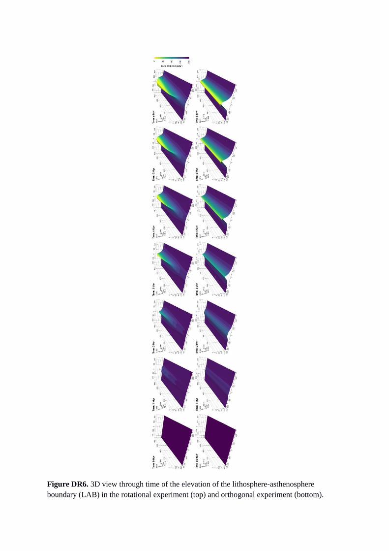
Figure DR6. 3D view through time of the elevation of the lithosphere-asthenosphere

boundary (LAB) in the rotational experiment (top) and orthogonal experiment (bottom).

Table DR1

Parameter Upper Crust Lower Crust Mantle

Reference density, 𝜌𝑟(kg m-3

) at 293.15 K 2800 2900 3300

Thermal expansivity, 𝛼 (K-1

) 3e-5 3e-5 3e-5

Heat capacity, 𝐶𝑝(J K-1

kg-1

) 1000 1000 1000

Thermal diffusivity, 𝛼(m2 s

-1) 1e-6 1e-6 1e-6

Latent heat of fusion, 𝐿𝑓(kJ kg-1

) 300 300 300

Radiogenic heat production, A (W m-3

) 1.2e-6 0.6e-6 0.02e-6

Melt density change fraction, 𝑀𝛥𝜌𝑟 0.13 0.13 0.13

Liquidus term 1, t1 (K) 1493 1493 2013

Liquidus term 2, t2 (K Pa-1

) -1.2e-7 -1.2e-7 6.15e-8

Liquidus term 3, t3 (K Pa-2

) 1.6e-16 1.6e-16 3.12e-18

Solidus term 1, t1 (K) 993 993 1393.661

Solidus term 2, t2 (K Pa-1

) -1.2e-7 -1.2e-7 1.32899e-7

Solidus term 3, t3 (K Pa-2

) 1.2e-16 1.2e-16 -5.104e-18

Friction coefficient 0.577 0.577 0.577

Softened friction coefficient 0.1154 0.1154 0.1154

Cohesion, C (MPa) 10 20 10

Softened cohesion, C (MPa) 2 4 2

Pre-exponential factor, A (MPa-n

s-1

) 6.60693e-8 10e-2 1600

Stress exponent, n 3.1 3.2 3.5

Activation energy, E (kJ mol-1

) 135 244 520

Activation volume, V (m3 mol

-1) 0 0 23e-6

Water fugacity 0 0 1000

Water fugacity exponent 0 0 1.2

Melt viscous softening factor 1e-3 1e-3 1e-1

Melt fraction range for viscous softening 0.2 - 0.3 0.2 - 0.3 0 - 0.02

Code and Experiment Inputs

Numerical code used

The version of Underworld used can be found at:

https://github.com/OlympusMonds/EarthByte_Underworld

This version of Underworld is a fork of Underworld 1.8, with some extras plugins to work

more smoothly with the Lithospheric Modelling Recipe.

We recommend new users of Underworld should use Underworld 2.0, found here:

https://github.com/underworldcode/underworld2

Experiment Inputs

The experiments were designed based off the Lithospheric Modelling Recipe (the LMR),

which is a set of pre-defined Underworld input files and a script framework to help run them.

The LMR can be found here:

https://github.com/OlympusMonds/lithospheric_modelling_recipe

The input files used in this experiment can be found here:

https://github.com/OlympusMonds/lmondy-et-al-3D-Rifting-Experiments

References Crameri, F., Schmeling, H., Golabek, G., Duretz, T., Orendt, R., Buiter, S., May, D., Kaus,

B., Gerya, T., and Tackley, P., 2012, A comparison of numerical surface topography

calculations in geodynamic modelling: an evaluation of the ‘sticky air’method:

Geophysical Journal International, v. 189, no. 1, p. 38-54.

Demouchy, S., Tommasi, A., Ballaran, T. B., and Cordier, P., 2013, Low strength of Earth’s

uppermost mantle inferred from tri-axial deformation experiments on dry olivine

crystals: Physics of the Earth and Planetary Interiors, v. 220, p. 37-49.

Dziewonski, A., Chou, T. A., and Woodhouse, J., 1981, Determination of earthquake source

parameters from waveform data for studies of global and regional seismicity: Journal

of Geophysical Research: Solid Earth, v. 86, no. B4, p. 2825-2852.

Ekström, G., Nettles, M., and Dziewoński, A., 2012, The global CMT project 2004–2010:

Centroid-moment tensors for 13,017 earthquakes: Physics of the Earth and Planetary

Interiors, v. 200, p. 1-9.

Ellis, S. M., Little, T. A., Wallace, L. M., Hacker, B. R., and Buiter, S. J. H., 2011, Feedback

between rifting and diapirism can exhume ultrahigh-pressure rocks: Earth and

Planetary Science Letters, v. 311, no. 3-4, p. 427-438.

Floyd, J. S., Tolstoy, M., Mutter, J. C., and Scholz, C. H., 2002, Seismotectonics of mid-

ocean ridge propagation in Hess Deep: Science, v. 298, no. 5599, p. 1765-1768.

Hasterok, D., and Chapman, D., 2011, Heat production and geotherms for the continental

lithosphere: Earth and Planetary Science Letters, v. 307, no. 1, p. 59-70.

Hirth, G., and Kohlstedt, D., 2003, Rheology of the upper mantle and the mantle wedge: A

view from the experimentalists: Inside the subduction Factory, p. 83-105.

Koopmann, H., Brune, S., Franke, D., and Breuer, S., 2014, Linking rift propagation barriers

to excess magmatism at volcanic rifted margins: Geology, v. 42, no. 12, p. 1071-1074.

McKenzie, D., and Bickle, M., 1988, The volume and composition of melt generated by

extension of the lithosphere: Journal of petrology, v. 29, no. 3, p. 625-679.

Paterson, M., and Luan, F., 1990, Quartzite rheology under geological conditions: Geological

Society, London, Special Publications, v. 54, no. 1, p. 299-307.

Rey, P., and Müller, R., 2010, Fragmentation of active continental plate margins owing to the

buoyancy of the mantle wedge: Nature Geoscience, v. 3, no. 4, p. 257-261.

Van Wijk, J. W., and Blackman, D. K., 2005, Dynamics of continental rift propagation: the

end-member modes: Earth and Planetary Science Letters, v. 229, no. 3-4, p. 247-258.

Wang, Y., Zhang, J., Jin, Z., and Green, H., 2012, Mafic granulite rheology: Implications for

a weak continental lower crust: Earth and Planetary Science Letters, v. 353, p. 99-107.

Watremez, L., Burov, E., d'Acremont, E., Leroy, S., Huet, B., Pourhiet, L., and Bellahsen, N.,

2013, Buoyancy and localizing properties of continental mantle lithosphere: Insights

from thermomechanical models of the eastern Gulf of Aden: Geochemistry,

Geophysics, Geosystems, v. 14, no. 8, p. 2800-2817.

Zhong, S., and Watts, A., 2013, Lithospheric deformation induced by loading of the

Hawaiian Islands and its implications for mantle rheology: Journal of Geophysical

Research: Solid Earth, v. 118, no. 11, p. 6025-6048.