1

The Role of Costs for Postal Regulation

John C. Panzar

University of Auckland and Northwestern University

1. Introduction and Summary

The purpose of this White Paper is to analyze the Cost and Revenue Analysis (CRA)

costing framework developed by the Postal Service and its regulators over the past several

decades with the objective of carefully explaining how various Postal Service cost measures can

be used to guide the Postal Rate Commission (PRC) in fulfilling its pricing responsibilities, as

specified in 39 U.S.C. 3622(c)(2) and 39 U.S.C. 3633(a). Essentially, these statutory provisions

require that prices be set so that:

(i) Each market dominant product bears the costs “attributable” to it through

“reliably identified causal relationships.”

(ii) The market-dominant products of the Postal Service do not subsidize its

competitive products.

(iii) The competitive products, taken together, cover an “appropriate share of the

institutional costs of the Postal Service.”

Meeting this goal requires us to carefully explain how Postal Service cost concepts such as

volume variable costs, infra-marginal costs and institutional costs are related to established

economic cost concepts such as marginal costs, incremental costs, fixed costs and variable costs.

Perhaps most importantly, we must determine the economic meaning of the statutory term

2

“attributable” and relate it to the concept of attributable costs as defined by the Postal Service in

the CRA.

The paper presents a thorough discussion of the relevant multiproduct economic cost

concepts, cost causality, and the workings of the CRA. However, the results of our analysis can

be succinctly stated as follows:

(1) The statutory use of “attributable” clearly specifies that there be a causal relationship

between the product provided and the costs attributed to it. Identifying the relevant

economic cost condition is equally straightforward: the costs caused by a product (or

group of products) are, by definition, the incremental costs of that product (or group

of products). Therefore, statutory attributable costs should be interpreted as

economic incremental costs. Thus, the PRC should use estimates of product

incremental costs in order to meet the pricing responsibilities discussed above.

(2) The CRA methodology defines attributable costs in a way that only partially aligns

with the economic definition of incremental costs. In general, CRA attributable costs

understate economic incremental costs.

(3) Fortunately, the accounting data generated by the CRA can be used to calculate the

economic incremental costs of Postal Service products.

Our conclusions are based upon more than two decades of economic research on postal

costing methodology. Postal Service costing is designed to deal with the multiservice nature of

postal operations. That is, it attempts to trace the impacts of specified service levels (volumes)

on the levels of “cost drivers” required to meet them. It does so by specifying for each service a

relationship between service volumes and driver activity for each of several cost components.

Bradley, Colvin and Smith (1993) first explained the relationship between Postal Service costing

relationships and economic concepts such as marginal cost. Subsequent work by Bradley,

3

Colvin and Panzar [(1997), (1999)] further explained how Postal Service cost accounts can be

used to calculate the incremental cost of various services. This White Paper builds on this earlier

work.

The remainder of this White Paper proceeds as follows. Section 2 provides a review of

the economic multiproduct cost concepts required for our analysis.1 Particular emphasis is

placed upon the concept of incremental cost and its connection to cost causality. Section 3

presents a brief outline of the CRA costing methodology used by the Postal Service. Section 4

briefly reviews the cost concepts required to implement the pricing responsibilities of the PRC.

In Section 5 we develop a simple example to illustrate the workings of the CRA. This

framework allows us to clearly explain the relationships between postal constructs such as

volume variable costs and attributable costs to standard economic cost measures. We further

develop our example to illustrate how the data generated by the CRA can be used to inform

economic policy issues related to pricing and cross-subsidization. Our final section offers a brief

Conclusion.

2. Multiproduct Cost Functions and Cost Causality

To an economist, there is a causal relationship between the quantities of various

economic goods and services provided and the expenditures incurred by the entity producing

those goods and services. In economic textbooks, this relationship is usually defined as the

solution to an explicit optimization problem: i.e., it is assumed that the amount of inputs chosen

by the firm, x = (x1, x2, …, xm), are chosen so as to minimize the total expenditures required to

1 The reader is referred to Baumol, Panzar and Willig (1988) and Panzar (1989) for more detailed discussions.

4

produce a vector of specified output levels, Q = (Q1, Q2, …, Qn).2 However, for purposes of the

present discussion, it is only necessary that there exists a relatively stable relationship between

inputs, outputs and factor prices so that one can assume that there exists a multiproduct Postal

Service behavioral cost function,

relating the levels of services provided

and input prices to the resulting amount of costs incurred.3 In what follows, we will assume that

the factor prices facing the Postal Service are exogenously fixed, so that the relationships of

interest can be summarized by the function C(Q). We also assume that the cost relationships

under discussion are (what economists refer to as) long-run costs.4

We will make extensive use of the following standard economic cost concepts and basic

definitions:

Definition E1: TOTAL COSTS. The function C(Q) measures the total costs caused by the

production of the specified quantities of all products produced by the firm. Total Costs are

causally related to the output vector Q, because they would all vanish if Q did.

2 More formally, let the vectors

and , respectively, denote output levels of the various goods and

services offered by the firm and the quantities of the inputs used to produce them and let denote the vector

of positive input prices facing the firm. Then, the solution to the firm’s cost minimization problem defines the

minimum cost function ̃

as ̃( ) . See, for

example, the treatments in an advanced microeconomic textbook such as Mas-Colell, Whinston and Green (1995).

3 In testimony before the Commission, Panzar (1997) has described in some detail how such a behavioral cost

function can be viewed as the result of the implementation by the Postal Service of a well-specified (although not

necessarily cost-minimizing) Operating Plan.

4 Long-run costs are sometimes referred to as “drawing board costs.” They are the expenditures that would be

incurred to provide the specified vector of output quantities if the firm were able to “start from scratch,” not

burdened by legacy facilities or labor contracts.

5

This cost function is assumed to be defined for any nonnegative output vector Q > 0. However,

it is customary to use a special terminology for the costs associated with output vectors in which

one or more output levels are equal to zero. A bit of additional notation is needed to define total

costs for proper subsets of products. Given any reference output vector Q > 0 in which all n

products are produced in strictly positive quantity, let QS denote that vector whose ith component

is equal to that of the reference vector Q for iS and equal to 0 for iS. Thus, Q = QS + QN/S,

where the set N/S {iN | iS} is the complement of S in N. We are now able to state:

Definition E2. STAND ALONE COSTS. The stand alone costs of any product set SN and its

complement N/S are given by C(QS) and C(QN/S), respectively. Stand alone costs are jointly

caused by all of the products in the subset in question.

The important economic implications of C are contained in a complete description of

how costs change in response to a change in the levels of the services provided. Economists

refer to these cost changes as:

Definition E3. INCREMENTAL COSTS. The incremental costs of any vector of changes in

output levels or volumes, Q = (Q1, Q2, …, Qn), relative to a base vector Q0 of total output

is the amount of costs that would be avoided if Q were no longer produced. That is, IC(Q0;Q)

= C(Q0) – C(Q

0–Q). Incremental costs are jointly caused by all of the changes in all of the

products involved in Q.

Other familiar cost concepts can be constructed from this definition through artful

choices of the increment, Q. (Unless otherwise specified, the base vector, Q0, is taken to be the

total output vector Q.) For example, the marginal cost of service i, MCi(Q), results from

choosing the increment Q = (0, 0, …, Qi, …, 0) and taking the limit of IC/Qi as Qi goes to

zero. The incremental cost of a particular product or service, say service i, ICi, is obtained by

choosing the increment to be all units of that service (and only that service). In that case, we

assume that Q = (0, 0, Qi, …, 0) so that ICi = C(Q) – C(QN/i) . Similarly, the incremental cost

6

of a set of services SN results from choosing the increment Q = QS. Thus, ICS(Q) = C(Q) –

C(QN/S) = C(QS+QN/S) – C(QN/S).

The economic concept of incremental costs is central to any notion of cost causality. To

say that service (or group of services) X causes an expenditure Y is equivalent to saying that Y is

the Incremental Cost of X. Regulatory statues do not always explicitly refer to the above,

economic definition, of Incremental Cost. However, most statutes are explicitly concerned with

the concept of cost causality, using the term much as an economist would. One of the clearest

(and most succinct) definitions we have come across is due to the Illinois Commerce

Commission

(Title 83, Section 791.30, Cost Causation Principle):

Costs shall be attributed to individual services or groups of services based on the

following cost causation principle. Costs are recognized as being caused by a

service or group of services if:

a) The costs are brought into existence as a direct result of providing the

service or group of services; or

b) The costs are avoided if the service or group of services is not provided.

The parallel emphasis on the concept of avoided cost is particularly important as a guide to

intuition. Since costs are frequently “brought into existence” by a number of different products

or services, it is possible to get caught up in a “chicken and egg” confusion based upon

hypothetical scenarios concerning the order in which products were introduced into the firm’s

portfolio. Indeed, the costs of adding a particular product (or group of products) will differ

depending upon the mix of products already present. However, it is unambiguously clear that

the only added costs that are equal to avoided cost are those that result when the product (or

group of products) in question is added last. And, that is precisely the cost measured by the

economic definition of Incremental Costs, as presented in Definition E3.

Finally, economists often find it necessary to distinguish between variable costs that vary

continuously with volume and fixed costs that do not. To make this distinction it is useful to

assume that our basic cost function C(Q) can be rewritten as follows:

7

( ) ( ) (1)

Here, the function is usually assumed to be increasing and twice continuously

differentiable, with V(0) = 0. Let the set SN denote that subset of services that are produced in

strictly positive quantities. That is, . Define the “fixed cost function”

to have the following intuitive properties. First, long-run fixed costs are zero when

there are no services provided: i.e., . Second, the level of fixed costs increases as the

set of services offered includes more and more products: i.e., for

. We can now formally state the following definitions:

Definition E4. VARIABLE COSTS. The function V(Q) measures the variable costs of the firm:

i.e., those costs that vary continuously with volume.

Definition E5. FIXED COSTS. The fixed costs of the firm are those that must be

(discontinuously) incurred as any positive amount of output is produced. (That is why fixed

costs are sometimes referred to as “start up costs.”) The function F{S} allows the amount of the

start-up costs to vary with the set SN of products introduced.

The division of costs into “fixed” and “variable” categories can be carried over to any of

the cost concepts defined above. For example, the fixed portion of the Incremental Cost of

product i is given by F{N} – F{N/i}, the difference between the amount of fixed costs that arise

when all products are produced and the amount of fixed costs that remain when the production of

product i is discontinued. The variable portion of the Incremental Cost of product i is similarly

defined using the variable cost function: i.e., V(Q) – V(QN/i).5 Thus, the basic formula for the

total incremental cost of product i can always be rewritten as the sum of its fixed and variable

portions:

5 The expressions for the fixed and variable portions of the incremental costs associated with subsets of products are

similar. These are, respectively, given by and ( ) ( ).

8

[ ( )] [ ( )] [ ] [ ( ) ( )] (2)

A brief digression on the nature of the fixed costs discussed in our analysis is necessary.

As noted earlier, our discussion is devoted entirely to the case of long-run costs. Yet, some

readers may recall (perhaps from a course in Introductory Economics) seeing the maxim: “Fixed

costs are zero in the long-run.” That maxim reflects the fact that, when all input levels can be

freely adjusted (i.e., the economist’s long-run), the cost of producing nothing must, by definition,

be nothing. That is, C(0) = 0. Nothing here contradicts that basic tautology. The fixed costs

considered here could perhaps more descriptively be referred to as “start-up costs” that measure

the size of “jump discontinuities at the origin.” These are the significant levels of costs that must

be incurred in order to produce even a vanishingly small level of output.6

3. Brief Review of Postal Service Costing (CRA)

The Postal Service employs a product costing methodology to generate cost information,

both for internal decision making and to satisfying the cost reporting requirements of the PRC.

This costing system is referred to as Cost and Revenue Analysis (CRA).7 The CRA models total

costs by dividing the incurred expenses of the enterprise into some number of cost components,

indexed by j = 1, …, J. The expenditures associated with the jth cost component, , are

6 Think of a railroad-building project at the “drawing board stage.” The planned costs to produce zero output –

walking away from the project – would indeed be zero. However, if the plans called for the production of a very,

very small level of output, say one-ton mile of A to B transportation, the planned costs would not be “close” to zero.

They would include millions of dollars to purchase the right of way, prepare the roadbed, lay the track, etc. This is

the kind of situation economists have in mind when referring to the presence of “fixed costs” in the “long-run.”

7 See Bradley, Colvin and Smith (1993) and RARC (2012a) for a detailed description of Postal Service costing

methodology, as reflected in its Cost and Revenue Analysis (CRA) reports. Here, we present only a basic

description of the CRA in order to illustrate the issues at hand.

9

assumed to be caused by the level of the cost driver, , associated with that activity: that is,

( ). Let denote the marginal cost of component j, the increase in

component cost caused by a marginal increase in component driver activity. The level of the

cost driver is determined by the volumes of individual mail products ( ).

Thus, the CRA analyzes Postal Service cost by characterizing the behavior of component

costs with respect to their cost drivers and then distributing the resulting cost pools to individual

products based upon their impacts on the level of driver activity. For example, one important

component of postal costs is transportation costs. On a particular route, transportation costs are

primarily determined by the total volume, in cubic inches, of all mail products transported. The

component costs are then specified as a function of the number of cubic inches transported.

Thus, for transportation costs, the number of cubic inches is the level of cost driver activity. The

total number of cubic inches required for transportation is determined by the number of cubic

inches per piece of each type of mail product and the number of pieces of each type transported.

3.1 Volume Variability of Cost Components

The CRA analysis begins by determining the proportion of component costs that are

“volume variable” with respect to the level of the cost driver. In postal parlance, this is done by

applying a “variability factor” to total component costs. In economic terms, this variability

factor is simply the elasticity, ( ), of total component costs with respect to component driver

activity. This elasticity is defined as the percentage change in total component costs divided by

the percentage change in driver activity:

( )

(3)

10

The volume variable costs of component j, , are then obtained by multiplying total

component costs by the variability factor:

[

] ( ) (4)

This process is essentially a method of reflecting the economies of scale associated with a

particular cost component. If component costs rise less than proportionately with driver activity

( ), an economist would say that the component was characterized by increasing returns to

scale. A postal analyst would say that the component’s volume variability was less than 100%.

Definition P1: COMPONENT VOLUME VARIABLE COSTS. The volume variable costs

associated with a cost component are equal to the elasticity of component cost with respect to

driver activity multiplied by total component costs.

It is important to emphasize that volume variable costs are not equivalent to the economic

concept of variable costs, defined above. In order to clarify this issue, it is useful to rewrite total

component costs as the sum of its fixed and variable components:

( ) ( ) (5)

Here, component fixed costs, Fj, and component variable costs, ( ), correspond exactly to

the economic concepts presented in Definitions E4 and E5. Component fixed costs are “start-

up” costs that must be incurred to provide even an arbitrarily small level of driver activity.

Component variable costs consist of those component expenditures that vary continuously with

the level of driver activity. Differentiating equation (5) with respect to yields ,

the condition that marginal component cost equals marginal variable component costs. This

allows us to rewrite equation (2) as

( ) ( ) (6)

11

Therefore, the difference between postal component volume variable costs and the economic

concept of component variable costs is given by ( ) ( ). Only in the case of

constant component marginal costs will this difference be zero. Component volume variable

costs will always be less than component variable costs whenever component average variable

costs are decreasing (and, hence, greater than component marginal cost).

As we shall see, defining volume variable costs at the component level is a very useful

step toward obtaining estimates of marginal cost from cost accounting data. However, it creates

another category of costs, i.e., component infra-marginal costs, , requiring specialized

postal terminology:

Definition P2: COMPONENT INFRA-MARGINAL COSTS. The infra-marginal costs associated

with a cost component are equal to component variable costs minus component volume variable

costs. That is, ( ) ( ) ( ) ( ) ( ).

Infra-marginal costs are not a standard economic cost concept. Essentially, they are defined by

what they are not: i.e., they are variable costs that are not volume variable costs.

3.2 Distribution of Component Costs to Individual Postal Products

After the component volume variable costs are determined, they are assigned, or

distributed, to individual products based upon a specified relationship between product volumes

and the level of component driver activity. The level of the cost driver is assumed to be

determined by the volumes of individual mail products; i.e., Dj = D

j(Q). Cost drivers are

typically defined in such a way that the functions Dj are linearly homogeneous, so that a

proportional increase in all volumes leads to an increase of driver activity of the same

proportion: i.e., Dj(tQ) = tD

j(Q) for any constant t > 0. Often, the relationship is assumed to be

linear, so that Dj(Q) = mQ = imiQi for some vector of product weights m = (m1, …, mn). For

12

example, suppose that cubic inches are recognized as the cost driver for the transportation cost

component and that there are two services “letters” and “parcels.” If each letter occupies ml

cubic inches and each parcel mp cubic inches, the total amount of the cubic inches cost driver is

given by: Dcube

= mlQl + mpQp.

The next step is to determine each product’s share, ( ), of the cost driver activity of

component j. When possible, this share is simply the estimated elasticity of component j driver

activity with respect to the volume of product i. That is,

( )

(7)

(By Euler’s Theorem, the linear homogeneity of Dj(Q) ensures that these shares sum to one.) In

practice, most of the driver relationships are assumed to be linear. The result is that each

product’s share is simply its (weighted) contribution to a (weighted) sum of outputs:

( )

∑ (8)

The determination of driver shares for a cost component makes it possible to distribute

any portion of the component’s cost to individual services.8 In the CRA, only a component’s

volume variable costs are distributed to individual products.9 The amount of component j

volume variable cost distributed to product i is given by:

8 Indeed, the vector of driver shares is sometimes referred to as a distribution key.

9 However, in principle, the same driver shares can be used to distribute any category of component costs: e.g., fixed

costs, variable costs and infra-marginal costs.

13

[

] [

]

(9)

However, it is important to avoid the temptation to view the volume variable costs distributed to

a particular product as being caused by that product. The variable costs of a component are

jointly caused by all the volumes of all the products that utilize that component. These costs

may be distributed to individual products based on that product’s share of driver activity.

However, unless component marginal cost is constant, the resulting cost distribution to product i

is not the amount of cost that would be avoided if product i were to be discontinued: i.e., it is not

the incremental cost of product i.

The total amount of volume variable cost attributed to any product i is determined by

summing its component volume variable costs distributions over all cost components:

∑

∑

(10)

The CRA expresses the volume variable costs distributed to service i on a per unit basis by

dividing VVCi by the volume of service i. That is,

( )

∑

[∑ [ ( ) ]

( ) (11)

The well-known10

outcome of the CRA’s volume variability analysis is the surprising result that

the unit volume variable cost of a service is equal to the marginal cost of that service.

The end result of the CRA process is the determination of the attributable costs, Ai, of

each individual postal product. This is obtained by adding any specific-fixed costs,11

Fi,

10

See, for example, Bradley, Colvin and Smith (1993) and Bradley, Colvin and Panzar (1999).

14

associated with the product to the product’s volume variable costs. This gives rise to another

specialized postal cost term:

Definition P3: ATTRIBUTABLE COSTS. The attributable costs of product i are equal to the sum

of that product’s specific-fixed costs and its volume variable costs: i.e., Ai = Fi + VVCi.

4. Economic Cost Concepts, “Postal” Cost Concepts and the Pricing Responsibilities of the Postal Regulatory Commission.

From an economic policy perspective, the primary purpose of a firm’s costing system is

to provide estimates of the marginal and incremental costs of the products sold by the firm.

4.1 Unit Volume Variable Costs are designed to measure Economic Marginal Costs

Marginal costs are an essential ingredient in the pursuit of any policy objective for the

firm. Regardless of the objective of the firm or its regulator, appropriate pricing policy must be

based upon reliable estimates of each product’s marginal cost. 12

Fortunately, the costing

methodology developed in the CRA is exceptionally well designed to provide the Commission

11

Interestingly, this is one case in which postal cost terminology coincides with standard economic usage.

Compare, for example, Bradley, Colvin and Smith (1993) and Panzar (1989). Specific-fixed costs are start-up costs

that arise when any positive amount of the service is provided. And, of course, these costs are avoided if the service

is discontinued. Specific-fixed costs do not vary with the product volume or the level of driver activity of any

component. The CRA typically assumes that specific-fixed costs are independent and additive. Thus, in terms of

equation (1) and Definition E5, we adopted the notation that Fi = F{i} and F{S} = FS = iS Fi.

12 The efficiencies associated with marginal cost pricing are a major topic of modern microeconomic theory, and

need no elaboration here. Of course, marginal cost pricing would result in losses for enterprises operating under

increasing returns to scale (such as the Postal Service). However, even in these cases, economically rational pricing

policies must utilize information on marginal costs. See, for example, the discussions in Viscusi, Harrington and

Vernon (2005) and Braeutigam (1989).

15

with accurate and detailed estimates of the marginal costs of Postal Service products. As

explained in the previous section, the CRA magnitude, unit volume variable cost, corresponds

exactly to the economic definition of marginal costs. Thus, the CRA’s “volume variability

approach” to costing provides accurate measures of marginal cost on a product by product basis.

In addition, this framework is especially useful for evaluating the profitability of product

offerings, such as Negotiated Service Agreements, that involve only small percentage changes in

Postal Service volumes.13

4.2 Product-level CRA Attributable Costs are not designed to measure product level Incremental Costs.

For the economist, the second role of cost analysis is to make it possible for prices to be

evaluated for cross-subsidization. It is now standard in the regulatory economics literature that

avoiding cross-subsidization means that the customers of each product (or group of products)

pay more to the firm in revenues than the incremental cost of said product (or group of

products).14

However, even today, not all regulatory statutes address cross-subsidy concerns

through explicit reference to the above-mentioned “incremental cost test.” Rather, they may use

language to the effect that revenues obtained from a product are such that

“ … each class of mail or type of mail service bear the direct and indirect postal costs

attributable to each class or type of mail service through reliably identified causal

relationships …”

13

See the analysis in RARC (2012b).

14 Again, see Viscusi, Harrington and Vernon (2005) or Braeutigam (1989).

16

The term “attributable” is commonly used in regulatory statues, but it has no precise economic

definition. However, as explained in Section 2, costs resulting from “causal relationships” can

only be measured as incremental costs.

Unfortunately, the attributable cost of a product, as developed by the CRA does not

adequately measure that product’s incremental cost. One portion of attributable cost, specific-

fixed cost, makes up precisely the fixed part of a product’s incremental cost. These are clearly

causal, since they would be avoided if the product were not produced. The difficulty is with the

notion of product-level volume variable costs. These are, in general, not equal to the variable

portion of a product’s economic incremental costs. The reason that a product’s CRA volume

variable costs are not generally equal to the costs that would be avoided if the product were

eliminated is quite intuitive. Essentially, the reason is that the CRA’s volume variability

approach takes the product’s economic marginal cost – which is, indeed, the avoided cost of the

last unit of output – and applies that amount to all the units of the product provided. But, these

infra-marginal units will not have the same amount of avoided costs associated with them unless

marginal costs are constant. The analysis of the next section explains this point in detail.

5. Volume Variable Costs, Incremental Costs and Infra-Marginal Costs in the CRA: an Illustrative Example.

In this section we explain the distinction between volume variable costs, incremental

costs and infra-marginal costs using a simplified CRA – type model in which there are n

services, , and only one cost component. This example generally reflects the

CRA framework, but greatly simplifies the discussion (and mathematical notation). Treating the

case of a single cost component is, surprisingly, not particularly restrictive because most CRA

analysis and computations takes place at the component level. The results are then aggregated.

17

The empirical analysis in our Task 2 Report applies the insights developed here to the products

and cost components used by the Postal Service.

The expenses incurred by any cost component are caused by the level of driver activity,

D, according to the formula:

( ) ( ) (12)

Here, v(D) denotes component variable costs, that portion of component costs that varies directly

with the level of cost driver activity. F denotes the level of any component fixed costs. These

are component costs that do not vary with the amount of driver activity (or with the volumes of

individual services). Our stylized CRA formulation also allows for the possibility that there may

be specific-fixed costs Fi. These costs do not vary with service volumes (or the level of driver

activity). However, they would disappear if the service in question were to be discontinued. The

level of driver activity, itself, determined by service level volumes, Qi. As discussed in the

previous section, the relationship D(Q) is usually assumed to be linear. For notational

simplicity, we will assume that the units in which service volumes are measured are chosen so

that all the weights mi are equal to one and D = Q1 + Q2 + … + Qn = Q.

It is now possible to express the costs of our stylized postal operator in terms of the

standard multiproduct cost function used by economists:

( ) ( ) ( ) ∑ ( ) (13)

As usual, total costs can be divided into two categories. Fixed costs are the sum of component

fixed cost and the various specific-fixed costs: F + F1 + F2 + … + Fn. In this example, the only

costs that vary with volume are the component variable costs, v.

18

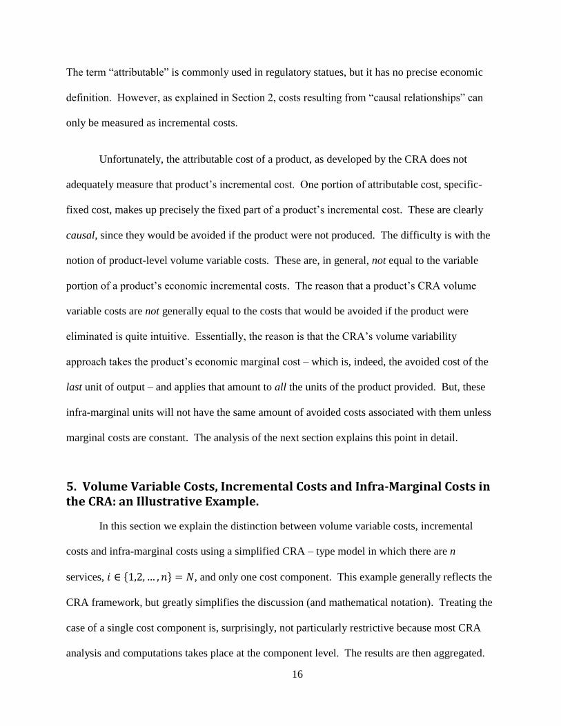
It is also possible to derive formulae for the standard economic cost concepts of (product)

marginal costs and (product) incremental costs for this example:

( )

( ) (14)

( ) ( ) ( ) ( ) ∫ ( )

(15)

It may also be necessary to consider the incremental costs associated with groups of products:

i.e., the product subsets SN. These are given by the following formula:

∑ ( ∑ ) ( ) (16)

These are all the cost measures an economist would need to set prices and test for cross-

subsidization. Notice that terms commonly used in postal costing discussions, such as

attributable costs, volume variable costs, and infra-marginal costs do not arise.

Next, we apply CRA costing methodology to our example. The central feature of the

CRA approach is the concept of volume variable cost, VVC. Again, it is important to point out

that, despite its name, VVC is not equivalent to the economic concept of variable costs. Rather,

the volume variable costs of a component are determined by applying a variability factor, , to

total component costs. This factor is obtained by estimating (econometrically or otherwise) the

elasticity of total component costs with respect to the level of cost driver activity. For the

present example, we have:

( )

( )

( )

( )

( ) (17)

and

19

( ) ( ) ( ) ( ) (18)

The nature of these postal cost concepts is illustrated in Figure 1, adapted from Bradley,

Colvin, and Smith (1993). The quantity of the cost driver is measured on the horizontal axis and

total component cost is measured on the vertical axis. Total component cost associated with

quantity 0D of the cost driver is given by the distance 0E. The distance 0A represents the

component's fixed cost. Constructing the tangent to the cost function at D, and extending it to

the vertical axis at point B, provides a measure of volume variable costs for this component.

These are given by the distance BE, which is equal to marginal component cost times the

quantity of the cost driver. Whenever marginal costs are a declining function of the level of the

cost driver, a component's volume variable costs will be less than its total variable costs (AE).

20

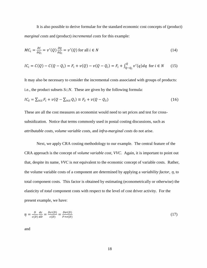
As explained above, “infra-marginal cost” is not a standard term in economic analysis. In

the postal costing literature,15

infra-marginal costs have ended up being defined in terms of what

they are not: i.e., volume variable costs. Thus, infra-marginal costs are that portion of

component variable costs that are not volume variable costs. In Figure 1, infra-marginal costs

for this component are given by the distance AB. That is, the difference between total

component variable costs AE and component Volume Variable Costs BE.

Of course prices are set for products, not cost drivers. Thus it is necessary to distribute

the total expenses of each cost component to the individual products of the enterprise. As

described above, this requires a specification of the relationship between the levels of service

volumes and the level of cost driver activity. In practice, this specification is often linear. In our

illustrative example the weights are equal to one, so that the level of driver activity is equal to the

simple sum of the service volumes: i.e., D = Q1 + Q2 + … + Qn = Q. Then, the portion of

volume variable costs that the CRA would distribute to each product is given by:

( ) (19)

As noted earlier, at the product level, per unit volume variable cost is precisely equal to marginal

cost:

( )

( ) ( ) (20)

15

See, for example, Bradley, Colvin and Panzar (1999).

21

Unfortunately, the postal costing process does not fully exploit this equivalence. Instead,

the CRA proceeds by adding a product’s specific fixed cost to its (distributed) volume variable

cost to obtain the product’s total attributable cost:

(21)

Dividing by service volume yields a measure of per unit attributable cost:

( )

( )

(22)

As is clear from the above discussion, ai differs from an economically valid measure of marginal

cost because it averages specific-fixed costs over service volume. Thus it is not a suitable

substitute for marginal cost for policy purposes. (Fortunately, the routinely calculated unit

volume variable cost is an accurate measure of marginal cost.)

Next, we explain why attributable cost is not an appropriate substitute for incremental

cost, the primary tool for determining whether prices are free of cross-subsidization. To see this,

subtract the above expression for attributable cost from that for the incremental cost of product i:

[ ( ) ( )] [ ( )] ∫ [ ( ) ( )]

(21)

The inequality follows from the fact that marginal component cost is decreasing. This means

that ( ) ( ) for all q < Q. Perhaps a more useful way to look at this result is as follows:

[ ( ) ( )] ( ) ∫ [ ( ) ( )]

(22)

The result can be seen more easily using Figure 2. Again, the level of driver activity is

measured along the horizontal axis. Now, the vertical axis measures the level of marginal

22

component cost . Two driver levels and the associated marginal costs are of interest: (i) the

level of marginal cost, ( ), evaluated at the total level of component driver activity when all

products are provided; and (ii) the level of marginal cost, ( ), that would result if service

i and its driver activity Qi were no longer provided. To simplify notation in the diagram, denote

the total amount of component driver activity that would occur without that caused by service i

by Q-i = Q – Qi.

Recall that the volume variable cost for service i are given by ( ) . This is the

rectangular area Q-i.QFE. The variable portion of the incremental cost of service i is the

difference between the total variable cost v(Q) less the variable cost v(Q-i) that would be incurred

if service i were not produced. Total variable component cost is, by definition, the area under the

component marginal cost curve up to Q, the level of total driver activity. Total variable

component cost without product i is the area under the component marginal cost up to Q-i, the

level of driver activity that would pertain without that due to product i. The variable portion of

incremental cost of product i for the component is the difference between the two: i.e., the area

Q-i.QFB under the component marginal cost curve between Q-i and Q. Finally, since the fixed

portions of attributable costs and incremental costs are identical (and equal to Fi), they cancel

out. The area BEF is difference between the variable portion of product i’s incremental cost and

its volume variable cost.

23

However, for plausible parameter values, it turns out that this difference is not large. In

the case in which component variable costs take on the constant elasticity form, the difference

between incremental costs and attributable costs is given by:

[ ( ) ] [ ( )

] (23)

or,

[ ( ) ] [ ( )

] (24)

Here, si is the share of total driver activity accounted for by service i. Table 1 presents values for

this difference as a percentage of component variable cost, i.e., the term in square brackets, for

various values of the cost elasticity and the driver share of service i.

24

share\elast 0 0.1 0.2 0.3 0.4 0.5 0.6 0.7 0.8 0.9

0 0.00% 0.00% 0.00% 0.00% 0.00% 0.00% 0.00% 0.00% 0.00% 0.00%

0.1 0.00% 0.05% 0.09% 0.11% 0.13% 0.13% 0.13% 0.11% 0.08% 0.05%

0.2 0.00% 0.21% 0.36% 0.48% 0.54% 0.56% 0.53% 0.46% 0.35% 0.19%

0.3 0.00% 0.50% 0.89% 1.15% 1.30% 1.33% 1.27% 1.09% 0.82% 0.46%

0.4 0.00% 0.98% 1.71% 2.21% 2.48% 2.54% 2.40% 2.06% 1.55% 0.86%

0.5 0.00% 1.70% 2.94% 3.77% 4.21% 4.29% 4.02% 3.44% 2.57% 1.41%

0.6 0.00% 2.76% 4.74% 6.03% 6.69% 6.75% 6.29% 5.34% 3.96% 2.16%

0.7 0.00% 4.34% 7.40% 9.32% 10.22% 10.23% 9.44% 7.95% 5.83% 3.16%

0.8 0.00% 6.87% 11.52% 14.30% 15.47% 15.28% 13.93% 11.59% 8.41% 4.51%

0.9 0.00% 11.57% 18.90% 22.88% 24.19% 23.38% 20.88% 17.05% 12.15% 6.41%

1 #NUM! 90.00% 80.00% 70.00% 60.00% 50.00% 40.00% 30.00% 20.00% 10.00%

Table 1

Difference between Incremental Costs and Attributable Costs as a function of Driver Share and

Component Cost Elasticity. (As a percentage of Component Variable Costs)

In Table 1, the rows indicate the fractional share of driver activity caused by the service

in question. Thus, a service that accounts for 30% of driver activity has a share of 0.3 in Table 1.

The columns indicate the elasticity of variable cost, for the cost component involved. The

items in the Table are expressed in percentage terms. Consider, for example, a product that

accounted for a 40% share of cost driver activity in a cost component with a cost elasticity of 0.8.

Its actual incremental cost would exceed its measured attributable cost by an amount equal to

1.55% of total component variable cost.

Table 1 reveals that the Postal Service measure of component attributable cost

understates the value of a product’s true incremental cost by only a small percentage amount.

For relevant parameter values (i.e., cost elasticity values greater than 0.5), this percentage

understatement decreases with the level of cost elasticity and increases with the product’s share

of driver activity. However, this understatement is less than 3% of component variable cost,

even in the case in which the cost elasticity is a very low 0.5 and the share of driver activity is a

very high 0.4. In any event, “correcting” Postal Service attributable costs to accurately measure

25

a product’s incremental cost should be a straightforward “spreadsheet calculation” based upon

available component cost information. Then, the PRC would have the information upon which

to base pricing policy (i.e., unit volume variable costs) and test for cross-subsidization at the

product level (i.e., incremental costs).

Indeed, an even more useful and surprising result is available for the important special

case in which component variable costs exhibit a constant elasticity: the closeness of the

approximation of attributable costs and incremental costs “aggregates” in a simple and intuitive

manner. This is an important result. It is well known that a complete test for subsidy free prices

is that revenues cover incremental costs not only for every individual product, but also for all

possible proper subsets of products. This is, in general, a daunting task because the number of

possible subsets of products increases with the factorial of the number of products.16

However,

the task is greatly simplified in the case of a constant elasticity component variable cost function

due to the additive structure of attributable costs.

The analysis is essentially the same as that above, however some additional notation is

useful. First, let denote the (proper) subset of postal products under

consideration. Next, let ∑ denote the total amount of component cost driver activity

accounted for by the product set in question. Finally, let ∑ denote the total share of

16

For example, for a firm with a product set consisting of 2 products, {1,2} there are only two

proper subsets to consider: {1} and {2}. However, for a firm with only 3 products there are six

proper subsets to consider: {1}, {2}, {3}, {1,2}, {1,3} and {2,3}. There 24 such subsets to

consider for a firm producing 4 products.

26

component driver activity accounted for by the products in S. Then the above equation relating

incremental costs and attributable costs for any product set S can be rewritten as:

∑ ∑ [ ( ) ] ∑ [ ]

[ ( ) ] (27)

or,

∑ [ ( ) ] (28)

Now, it is possible to use Table 1 to address most important pricing policy question facing the

Commission. That is, given information on how much volume variable cost has been attributed

and distributed to each product at the component level, it is straightforward to calculate an

estimate of the economically relevant incremental cost for each product and for any group of

products.

6. Conclusions

Attributable Costs as measured by the CRA have a serious shortcoming: they understate

incremental costs – the economically relevant standard for testing rates for cross-subsidization.

However, the CRA provides the necessary information to correct this shortcoming, allowing

incremental costs to be readily calculated.

27

REFERENCES

Baumol, William; John Panzar and Robert Willig (1988), Contestable Markets and the Theory of Industry

Structure, 2nd

Edition, Harcourt: New York.

Braetuigam, Ronald; “Optimal Policies toward Natural Monopolies,” (1989) Chapter 30 in Richard

Schmalensee and Robert Willig eds., Handbook of Industrial Organization Volume 2. Elsevier.

Bradley, Michael, Colvin, Jeff, John Panzar (1997), “Issues in Measuring Incremental Cost in a

Multi-Function Enterprise.” In M. Crew and P. Kleindorfer, eds., Managing Change in the

Postal and Delivery Industries, Kluwer.

Bradley, Michael; Jeff Colvin and John Panzar (1999), “On Setting Prices and Testing Cross-Subsidy

Using Accounting Data,” Journal of Regulatory Economics, 16: 83 – 100.

Bradley, Michael; Jeff Colvin and Mark Smith (1993), “Measuring Product Costs for Ratemaking: The

United States Postal Service.” In M. A. Crew and P. R. Kleindorfer eds., Regulation and the Nature of

Postal and Delivery Services. Kluwer Academic Publishers.

Office of the Inspector General, United States Postal Service, “A Primer on Postal Costing Issues,”

(2012a) RARC-WP-12-008.

Office of the Inspector General, United States Postal Service, “Costs for Better Management

Decisions: CRA Versus Fully Distributed Costs,” (2012b) RARC-WP-12-016.

Mas-Colell, Andreu; Michael Whinston and Jerry Green (1995), Microeconomic Theory.

Panzar, John; “Theoretical Determinants of Firm and Industry Structure.” Chapter 1 in Schmalensee and

Willig eds., The Handbook of Industrial Organization. Elsevier 1989.

Panzar, John (1997); Direct Testimony of John C. Panzar in Docket No. R97-1.

Viscusi, W. Kip; Joseph Harrington and John Vernon, (2005) Economics of Regulation and Antitrust,

MIT Press, 4th Edition.

28

Glossary of Terms and Mathematical Functions

Basic Notation

N = {1, 2, …, n} – denotes the set of all postal products

– denotes a particular subset of postal products

i – this subscript refers to quantities associated with a particular postal product

j – this superscript refers to quantities associated with a particular postal cost component

Qi – denotes the quantity provided of product i

– denotes the quantity of cost driver used in cost component j

Q = (Q1, Q2, …, Qn) – denotes the vector (list) of quantities of all postal products

QS = denotes a partial list of product quantities with arguments equal to Qi for iS and 0 for

iN/S.

Postal Cost Terms (and Associated Notation)

Variable Costs, ( ) – component costs that vary continuously with the level of cost driver

activity.

Variability Factor, ( ) – the percentage change in component j costs divided by the

percentage change in component driver activity.

Volume Variable Costs, – equal to Variable Costs multiplied by the elasticity of

component costs with respect to cost driver activity.

Fixed Costs, , – those component costs that do not vary with the level of driver activity.

Specific-fixed costs, , – costs that do not vary with the level of product volume or cost driver

activity, but would be avoided if the product were discontinued.

Attributable Costs (Product), Ai, – Specific-fixed costs plus Volume Variable Costs distributed to

the product based on its share of cost driver activity.

Infra-marginal Costs (Component), –Variable Costs minus Volume Variable Costs

Institutional Costs – Component Fixed Costs plus Infra-marginal Costs = Total Cost minus

Volume Variable Cost

29

Economic Cost Terms (and Associated Notation)

Total Cost, C(Q), – all the expenditures required to produce the specified levels of all of the

firm’s products

Incremental Costs, ICS(Q) – the costs that would be avoided if a product (or group of products)

were no longer produced = Variable Incremental Cost plus Product-Specific Cost

Stand Alone Cost, C(QS) – the costs of producing a subset of the firm’s products in isolation

Marginal Cost, MCi(Q) – the cost of producing an additional unit of product i

Variable Costs, V(Q) – those costs that vary continuously with the level of output

Marginal Variable Cost, MVi(Q) = MCi(Q) – the marginal variable cost of producing an

additional unit of product i. This always equals the marginal cost of product i.

Variable Incremental Costs – the variable costs that would be avoided if a product (or group of

products) were no longer produced

Elasticity of Variable Costs, – this parameter is the key cost parameter in the constant elasticity

example of Section 5.

Fixed Costs, F{S} – those costs that do not vary with the level of output