the role of high frequency intra-daily data, daily range ...period var forecasting using the s&p...
TRANSCRIPT

Munich Personal RePEc Archive
The role of high frequency intra-daily
data, daily range and implied volatility in
multi-period Value-at-Risk forecasting
Louzis, Dimitrios P. and Xanthopoulos-Sisinis, Spyros and
Refenes, Apostolos P.
Athens University for Economics and Business, BANK OF
GREECE, ATHENS
29 October 2011
Online at https://mpra.ub.uni-muenchen.de/35252/
MPRA Paper No. 35252, posted 07 Dec 2011 16:33 UTC
1
The role of high frequency intra-daily data, daily range and implied volatility in multi-
period Value-at-Risk forecasting
Dimitrios P. Louzisa,b,*, Spyros Xanthopoulos-Sisinisa and Apostolos P. Refenesa
Abstract
In this paper, we assess the informational content of daily range, realized variance, realized
bipower variation, two time scale realized variance, realized range and implied volatility in daily,
weekly, biweekly and monthly out-of-sample Value-at-Risk (VaR) predictions. We use the
recently proposed Realized GARCH model combined with the skewed student distribution for
the innovations process and a Monte Carlo simulation approach in order to produce the multi-
period VaR estimates. The VaR forecasts are evaluated in terms of statistical and regulatory
accuracy as well as capital efficiency. Our empirical findings, based on the S&P 500 stock index,
indicate that almost all realized and implied volatility measures can produce statistically and
regulatory precise VaR forecasts across forecasting horizons, with the implied volatility being
especially accurate in monthly VaR forecasts. The daily range produces inferior forecasting
results in terms of regulatory accuracy and Basel II compliance. However, robust realized
volatility measures such as the adjusted realized range and the realized bipower variation, which
are immune against microstructure noise bias and price jumps respectively, generate superior
VaR estimates in terms of capital efficiency, as they minimize the opportunity cost of capital and
the Basel II regulatory capital. Our results highlight the importance of robust high frequency
intra-daily data based volatility estimators in a multi-step VaR forecasting context as they
balance between statistical or regulatory accuracy and capital efficiency.
Jel Classification: C13; C53; C58; G17; G21; G32
Keywords: Realized GARCH; Value-at-Risk; multiple forecasting horizons; alternative volatility
measures; microstructure noise; price jumps.
a Financial Engineering Research Unit, Department of Management Science and Technology, Athens University of
Economics and Business, 47A Evelpidon Str., 11362 Athens, Greece.
b Bank of Greece, Financial Stability Department, 3 Amerikis Str., 105 64, Athens, Greece.
∗ Corresponding Author: E-mail address: [email protected]; [email protected]

2
1. Introduction
Precise assessment of financial risks plays a crucial role for the viability of the financial
institutions and the stability of the financial system as a whole. It helps minimizing the
probability of extensive periods of financial distress which may be triggered by the failure of
systemically important financial institutions. Obviously, the importance of accurate risk
measurement and assessment is augmented during highly volatile periods, such as the recent
2007-2009 financial crisis, for which there is a widespread risk of global financial instability
(Drakos et al., 2010).
This study concentrates on market risk which is defined as “the risk to a financial portfolio
from movements in market prices such as equity prices, foreign exchange rates, interest rates,
and commodity prices” (Christoffersen, 2003). The most popular market risk management tool in
the financial services industry is the so called Value-at-Risk (VaR), which reflects an asset’s
market value loss not be exceeded over a specified holding period, with a specified confidence
level (Alexander, 2008b). According to Giot and Laurent (2003b), the popularity of the VaR as a
market risk measure can be attributed mainly to three reasons. First, VaR is relative simple to
estimate – statistically, the α% VaR is α-th quantile of the conditional returns distribution.
Second, VaR is easy to communicate to higher level management as it encapsulates in a single
quantity, either percentage or nominal amount, the potential portfolio losses. Third, the 1996
market risk amendment to the Basel Capital Accord and the Basel II regulatory framework,
allows financial institutions to use their own internal VaR models for the calculation of market
risk capital requirements (see also subsection 3.3) (BCBS, 1996a, 2006). Thus, the extant
regulatory framework establishes the VaR as the benchmark method for market risk estimation.
The recent 2007-2009 global financial crisis and its subsequent widespread consequences in
the real economy highlighted once again the key role of financial volatility in financial assets’
risk management. During this turbulent period, characterized by extreme asset price movements
and high volatility in financial markets, the majority of financial institutions failed to comply
with the Basel Committee on Banking Supervision (BCBS) mandates regarding the accuracy of
their VaR estimates (Campel and Chen, 2008). This example from the near past financial history
underlines the need for accurate volatility measurement and forecasting and justifies the

3
intensive research efforts on measuring, modeling and forecasting financial volatility during the
last three decades .
In this study, we fill the gaps in the VaR related literature (see section 2) and we investigate
the informational content of three alternative classes of volatility measures in terms of multi-
period VaR forecasting using the S&P 500 stock index. The three volatility classes are: (i)
Range-based volatility estimators that employ the daily range, i.e. the difference between the
highest and lowest logarithmic prices within the trading day, and particularly the range estimator
of Parkison (1980). (ii) Realized volatility estimators, that utilize high frequency intra-daily
returns. In this category we use the realized variance (Andersen and Bollerslev, 1998; Andersen
et al., 2001a), the realized bipower variation which is robust against price jumps (Barndorff-
Nielsen and Shephard, 2004), the two time scale realized variance of Zhang et al. (2005) which
accounts for the microstructure noise bias in the price process and the realized range of and
Christensen and Podolskij (2007) and Martens and van Dijk (2007). (iii) Implied volatility as
measured by the VIX implied volatility index (Giot, 2005; Giot and Laurent, 2007). Each of the
abovementioned volatility estimators is based on different assumptions and informational sets
and differs in terms of efficiency, consistency and probably the ability to forecast the unobserved
volatility (Brownless and Gallo, 2010).
Here, we differentiate from previous works (see Section 2 for the related literature) and we
concentrate solely on the ability of the alternative volatility measures to deliver accurate and
efficient multi-step VaR forecasts. This practical approach for the evaluation of the informational
content of the various volatility measures requires the use of analogous evaluation metrics. Thus,
we do not restrict ourselves to only statistical accuracy evaluation of the VaR forecasts, i.e. via
the (un)conditional coverage tests of Christoffersen (1998), but we also use metrics that account
for the regulatory accuracy (Lopez, 1999) and the capital efficiency (Sharma et al., 2003) of the
VaR estimates. Finally, we also evaluate the alternative volatility measures in a real-world
setting utilizing the formula for the market risk capital requirements prescribed by the BCBS
(1996a, 2006).
Modeling the alternative volatility measures is another important issue of concern. The most
common approach is to use these volatility measures as lagged explanatory variables in a
GARCH model (Bollerslev, 1986) i.e. a GARCH-X model (e.g. Engle, 2002; Blair et al., 2001;
Giot, 2005; Fuertes et al., 2009; Corrado and Truong, 2007). However, the GARCH-X model

4
poses important limitations on our analysis as it can only produce day-ahead volatility or VaR
forecasts. Therefore, we use the novel Realized GARCH model proposed by Hansen et al.
(2011) and implemented in day-ahead VaR forecasts by Watanabe (2011), which is capable of
generating multi-period forecasts (see subsection 3.1). The Realized GARCH model is a relative
simple to estimate model that has the unique feature of joint modeling of realized volatility and
conditional volatility of returns, through a bivariate equation approach. Thus, the Realized
GARCH model eliminates the need for the two-step procedure usually implemented in the
realized volatility – VaR studies (Giot and Laurent, 2004; Brownless and Gallo, 2010). The
name of the model reflects its structure, which is similar to a GARCH model, and the fact that
incorporates realized volatility measures. Of course the model can be easily extended to allow
for alternative volatility measures.
Moreover, we follow Watanabe (2011) and we combine the Realized GARCH model with
the skewed student distribution for the innovations process which captures both the fat tails and
the asymmetry properties of the financial assets returns distribution (Fernadez and Steel, 1998;
Lambert and Laurent, 2001). These attractive characteristics and the good empirical performance
have popularized its use in day-ahead VaR applications (e.g. see Giot and Laurent, 2003a; Giot
and Laurent, 2003b; Giot and Laurent, 2004 and Giot, 2005 among others). However, forecasting
VaR at multi-period horizons is much more challenging than the day-ahead forecasts. The reason
is that we are not aware of the analytical form of the multiple horizons returns density
(Christoffersen, 2003). Hence, we utilize the numerical Monte Carlo simulation method in order
to estimate the multi-period VaR forecasts (Christoffersen, 2003; Andersen et al., 2006)
The rest of the paper is organized as follows. In Section 2 we provide the related literature,
while in Section 3 we describe the econometric methodology and the VaR evaluation metrics
used in this study. Section 4 presents the estimation results for the Realized GARCH model and
the VaR forecasting evaluation results. Section 5 summarizes and concludes this paper.
2. Related literature
A plethora of volatility measures and models have been used and tested in VaR estimation
and forecasting. The seminal Autoregressive Conditional Heteroscedasticity (ARCH) model of
Engle (1982), which uses the past squared daily returns in order to model the conditional

5
heteroscedasticity of financial assets returns, and its numerous extensions (e.g. see “Glossary to
ARCH (GARCH)” by Bollerslev, 2010) have been widely used in the VaR literature (e.g. see
Brooks and Persand, 2003; Angelidis et al., 2004; Kuester et al., 2006, Drakos et al., 2010
amongst others).
Nonetheless, since the introduction of the ARCH-type models, many alternative volatility
measures and models have been proposed for forecasting volatility and VaR. In particular, daily
range volatility estimators (e.g. see Parkison, 1980; Garman and Klass, 1983; Rogers and
Satchell, 1991) have also been employed in volatility (Chou, 2005; Li and Hong, 2011) and VaR
(Brownless and Gallo, 2010) forecasting studies. In these studies the range-based volatility
models outperform their GARCH counterparts. The intuition behind this result is that intraday
price ranges contain more information than the squared returns, since the latter are computed
from two arbitrary points in time, i.e. the closing prices (Chou et al., 2010). In Corrado and
Truong (2007), the authors find that the daily range and the implied volatility, as measured by
the VIX, VXO, VXN and VXD implied volatility indices, have similar volatility forecasting
performance. Chou et al., (2010) provide a good review on range-based volatility estimators,
models and their financial applications.
In the seminal papers of Andersen and Bollerslev (1998), Andersen et al. (2001a), Andersen
et al. (2001b) and Barndorff-Nielsen and Shephard (2002) the authors propose the sum of
squared intra-daily returns, the so called realized volatility, as an efficient and consistent
estimator of the latent volatility and they establish its asymptotic properties. The strong
theoretical foundations combined with the availability of high frequency intra-daily data initiated
a frenzy of research on realized volatility modeling and forecasting. In most of the volatility
or/and VaR forecasting empirical studies, the authors compare the ARCH-type to the realized
volatility models, or in other words, they examine if there is incremental information in high
frequency intra-daily returns compared to the daily squared returns.
In volatility forecasting studies the results are unequivocal; realized volatility models clearly
outperform their ARCH-type counterparts (e.g. see Andersen et al., 2003; Koopman et al., 2005;
Martens et al., 2009; Martens, 2002 amongst others). In VaR forecasting studies the results are
somewhat mixed with some authors providing evidence in favor of the realized volatility models
(Beltratti and Morana, 2005; Shao et al., 2009; Brownless and Gallo, 2010; Watanabe, 2011;

6
Louzis et al., 2011) and others reporting results in support of the ARCH-type models (Giot and
Laurent, 2004; Angelidis and Degiannakis, 2008; Martens et al., 2009).
Brownless and Gallo (2010) are the first to emphasize on the ability of alternative realized
volatility estimators to produce accurate day-ahead VaR forecasts. Using a P-spline
multiplicative error model (MEM) (for MEM models see Engle, 2002; Engle and Gallo, 2006),
the authors compare the predictive ability of realized variance, realized bipower variation, two
time scale realized variance, realized kernels (Barndorff-Nielsen et al., 2008) and daily range for
three NYSE stocks. Their results indicate that daily range and realized volatility estimators have
comparable forecasting behavior with volatility estimators that are robust against microstructure
noise performing relatively better. Moreover, Shao et al. (2009) provide evidence in favor of the
realized range compared to the realized volatility estimators in daily VaR forecasts. Watanabe
(2011) also report that the microstructure noise does not affect the accuracy of daily VaR
forecasts for the S&P 500 stock index. Alternative volatility estimators have also been used in a
volatility forecasting context. The majority of these studies favour the use of realized variation
measures that employ absolute intraday returns and, thus, can mitigate the effect of price jumps
(Forsberg and Ghysels, 2007; Ghysels et al., 2006; Ghysels and Sinko, 2006; Liu and Maheu,
2009; Fuertes et al., 2009; Louzis et al., 2012).
Another vigorously researched area in financial economics is concerned with the
informational content of implied volatility, which is deduced from options prices (see Alexander,
2008a). The majority of the studies in this area compare the volatility forecasts delivered by
models utilizing implied volatility measures with the forecasts generated by models employing
either daily range/squared returns or realized volatility estimators (e.g. see Blair et al., 2001;
Christensen and Prabhala, 1998; Corrado and Miller, 2005; Corrado and Truong, 2007; Giot and
Laurent, 2007 amongst others). Overall, implied volatility measures tend to outperform their
historical volatility counterparts in terms of volatility forecasting (Poon and Granger, 2003; Giot,
2005). However, despite its good forecasting performance, implied volatility measures have not
been broadly examined in risk management applications. The only exception is Giot (2005) who
is the first to investigate the predictive ability of implied volatility indices (the old VIX, VXO
and VXD corresponding to the S&P 500, S&P 100 and Nasdaq stock indices) in daily VaR
forecasts. His empirical analysis shows that implied volatility indices can provide accurate day-
ahead VaR forecasts when combined with the skewed student distribution.

7
Against this background, our work complements and extends previous empirical studies (e.g.
Brownless and Gallo, 2010; Giot, 2005; Watanabe, 2011; Shao et al., 2009) for several aspects.
First, this the first study that examines simultaneously the informational content of realized
volatility, daily range and implied volatility measures in a VaR forecasting context. Second, with
the exception Beltratti and Morana (2005), all other studies focus on day-ahead VaR forecasts.
Here, we also investigate the predictive ability of the alternative volatility measures at weekly,
biweekly and monthly horizons. Multi-step VaR estimates are quite important for both
regulatory, as Basel II framework requires the computation of 1% VaR for a ten-days holding
period, and internal risk management purposes. Third, we estimate the Realized GARCH using
volatility measures other than the realized volatility. Particularly, we extend the Realized
GARCH model in order to incorporate the realized bipower variation, the realized range, the
daily range and the implied volatility measures. Fourth, we propose the use of a Monte Carlo
simulation technique in conjunction with the Realized GARCH model in order to obtain the
multiple horizon returns density. Finally, we investigate the out-of-sample VaR forecasting
ability of the alternative volatility measures using eight years of the S&P 500 stock index which
include the challenging 2007-2009 crisis period. The empirical results concerning this period are
quite limited.
3. Volatility measures
In this section we briefly describe the three distinct categories of volatility measures
employed in this study. The first category comprises the daily range volatility estimator of
Parkison (1980) given by ( )1/ 4 log 2tRNG = ( )2log logt tH L− , where tH and tL are the high
and low daily prices respectively. Range-based volatility estimators have certain appealing
features in real-world applications. They are simple to estimate, more efficient than the squared
returns volatility proxy and robust against the microstructure noise bias (e.g. see Parkison, 1980;
Garman and Class, 1980; Alizadeh et al., 2002; Shu and Zhang, 2006).1
In the second category we examine volatility estimators that utilize ultra high frequency
intra-daily data. The most popular estimator in this category is the realized variance (RV)
1 Microstructure noise may take the form of bid-ask bounce, screen fighting, price discreteness and irregular trading (Fuertes et al., 2009).

8
(Andersen and Bollerslev, 1998; Andersen et al., 2001a; Barndorff-Nielsen and Shephard, 2002)
calculated as ( )∑ == M
j jtt rRV1
2, , where M is the total number of intraday returns for each day t
and ,t jr is the jth intraday return of day t . Under certain semi-martingale assumptions and for
∞→M , RV converges in probability to the quadratic variation of the price proces i.e.
p
t tRV QV→ 2 2
11
( ) ( )t
tt s t
s ds sσ κ−
− < ≤
= + ∑∫ , where the first part of the summation is the continuous
path component, or integrated variance ( tIV ) and the second part is the sum of squared jumps.
The realized bipower variation (RBV) of Barndorff-Nielsen and Shephard (2004) is a robust
estimator against price jumps and is given by ∑ += −= M
kj kjtjtt rrRBV1 ,,)2/(π , where 1=k . The
authors show that the RBV converges in probability to the continuous component of the
quadratic variation of the price process, i.e. 2
1( )
p t
t tt
RV IV s dsσ−
→ = ∫ and thus prove its immunity
to price jumps.
The two time scale realized variance (TTS-RV) estimator of Zhang et al., (2005) utilizes
both high and low frequency intra-daily data combined with sub-sampling in order to eliminate
the microstructure noise bias. Their estimator is - tTTS RV = ( ),(1/ )t
RV λλ
ΛΛ −∑ ,( / )f f f tM M RV ,
where ( ) tRV ,λ is the low frequency realized variance estimator for the subsample λ , given that
the full gird of the high frequency returns is partitioned into Λ= ,...,1λ , non-overlapping sub-
grids (e.g. 5=Λ if the low frequency is 5 minutes), tfRV , is the high frequency realized
variance estimator using the full grid, ( ) Λ+Λ−= /)1( λMM f is the average number of
observations in the subsamples and ( )λM is the total number of intraday observations in each
subsample set λ . The rationale behind the TTS-RV estimator is that since the microstructure
noise induced bias of the low frequency estimates is a function of the noise variance in the return
processes, which is in turn consistently estimated by the high frequency realized variance
estimator, we can use the latter in order to eliminate the low frequency estimator bias.
The realized range (RR) of Christensen and Podolskij (2007) and Martens and van Dijk
(2007) is the ‘realized version’ of Parkison’s range volatility estimator and is calculated as
( ) ( )2
, ,11/ 4 log 2 log log
M
t t j t jjRR h l
== −∑ , where jth , and jtl , are the high and low prices of the

9
jth time interval respectively. In Martens & van Dijk (2007), the authors propose the use of a
scaling factor in order to adjust the RR estimator for the microstructure noise bias. The scaling
factor is a ratio of the average value of daily range, tRNG , and the average value of RR and the
adjusted RR is given by ( )66 66
1 1t t k t k tk kRR RNG RR RR− −= =
= ∑ ∑ . Martens and van Dijk (2007)
show that the scaled RR outperforms the TTS-RV estimator in terms of efficiency.
Finally, in the third category, we assess the informational content of the implied volatility
(IV) measure which is deduced from options prices. We follow Giot (2005), Giot and Laurent
(2007) and Becker et al. (2009) and we use the VIX index, provided by the Chicago Board of
Options Exchange (CBOE), as a model-free IV measure. The VIX index is computed from a
number of put and call options on the S&P 500 index over a wide range of strike prices and is
designed to provide market’s expectation for the level of the S&P 500 volatility over the next 30
(22) calendar (trading) days(CBOE, 2003).2 Since VIX is reported in an annualized standard
deviation form, the daily IV measure is given by tIV = ( )2(1/ 365) tVIX (Giot, 2005; Giot and
Laurent, 2007).
4. Econometric methodology
4.1. The Realized GARCH model
The VaR forecasts are generated using the recently proposed Realized GARCH of Hansen et
al. (2011). Assuming that ( )1log /t t tr P P−= are the daily logarithmic returns, where tP is the
closing price of day t, the AR(1)- logarithmic Realized GARCH(1,1) is defined as:
1 1t t t tr c r h zφ −= + + , with tz ~ i.i.d skst(0,1,ξ,ν) (1)
1 1t t th h xω β γ− −= + + (2)
( )2
1 2 1t t t t tx h z zκ π τ τ ε= + + + − + , with tε ~ i.i.d N(0, 2
εσ ) (3)
2 We use the new VIX index of CBOE released on September 22, 2003. For technical details for the construction of the VIX index see CBOE White Paper (2003).

10
where tz are distributed as a standardized skewed student (skst) distribution with 2ν > and
0ξ > being the degrees of freedom and the asymmetry parameter respectively (Fernadez and
Steel, 1998; Lambert and Laurent, 2001), log( )t th h= and log( )t tx x= with
, , , - , or t t t t t t tx RNG RV RBV TTS RV RR IV= being the volatility measures presented in section 2.
The parameter 1τ captures the asymmetric impact of negative shocks on volatility process, i.e.
the leverage effects, and is expected to be negative, while 2τ captures the size effects or
volatility clustering i.e. the fact that large shocks tend to be followed by large shocks, and is
expected to be positive. Finally, the errors in equation (3), tε , are normally distributed and
mutually independent with tz .
We chose to model the conditional mean in equation (1), i.e. ( )1 1 1t t tE r c rF φ− −= + , as an
AR(1) process in order to account for any autocorrelation in the returns series while we follow
Watanabe (2011) and we assume the skewed student distribution for the innovations distribution,
which captures both the fat tails and the asymmetry properties of the financial assets returns
density. Moreover, the use of the logarithms ensures the positivity of the conditional volatility
estimates and retains the ARMA structure of the ‘GARCH equation’ or equation (2).
Nevertheless, the key feature of the Realized GARCH model is equation (3) or ‘measurement
equation’. It relates the volatility measures, tx , with the latent conditional variance,
( )1t t th Var r F−= , and enables the joint modelling of volatility measures and returns, which is a
very important aspect for empirical VaR applications. Moreover, in contrast with the GARCH-X
model, the Realized GARCH model can produce multi-period volatility – and consequently VaR
– forecasts via the measurement equation. For example, assume that we want to forecast the log
conditional variance for 2t+ i.e. 2 1 1 t t th h xω β γ+ + += + + . Hence, we need a forecast for 1th +
which is easily given by 1t t th h xω β γ+ = + + and a forecast for 1tx + which is given by the
measurement equation as follows: 1tx + = 1thκ π ++ + 1 1tzτ + ( )2
2 1 1tzτ ++ − 1tε ++ =
( )t th xκ π ω β γ+ + + + ( )2
1 1 2 1 11t t tz zτ τ ε+ + ++ − + . Finally, the measurement equation accounts for
possible biases of the alternative volatility measures. In general, we expect that an unbiased

11
estimator of the true daily volatility will produce estimates of κ close to zero and of π close to
one (see also the discussion in subsection 4.1).
All three equations’ parameters are estimated simultaneously by maximizing the joint log
likelihood of the Realized GARCH model, i.e.:
( ) ( ) ( )1 1
1
log , ; log ; log , ;skst n
t t t t t t t
t
r x f r x f x x rΤ
− −=
= +∑θ θ θL (4)
( )
( ) ( ) ( )
11
2
2
22
2
1 2 log log 0.5log 2 log
2 2
log( ) 0.5 log exp 1 log 12
0.5 log(2 ) log( )
t
t
Indt
t
t
sz ms h
εε
ν ν π νξ ξ
ν ξν
επ σσ
Τ
−=
−
⎛ ⎞+⎛ ⎞ ⎛ ⎞= Γ − Γ − − +⎡ ⎤⎜ ⎟ ⎜ ⎟ ⎜ ⎟⎣ ⎦ +⎝ ⎠ ⎝ ⎠ ⎝ ⎠⎧ ⎫⎡ ⎤+⎪ ⎪⎡ ⎤+ − + + +⎢ ⎥⎨ ⎬⎣ ⎦ −⎢ ⎥⎪ ⎪⎣ ⎦⎩ ⎭
⎡ ⎤− + +⎢ ⎥
⎣ ⎦
∑
where ( )1 1 2, , , , , , , , , , ,c εφ ω β γ κ π τ τ σ ν ξ ′=θ is the parameters vector, ( )1;skst
t tf r x − θ and
( )1, ;n
t t tf x x r− θ is the skst and the normal density function respectively, ( ).Γ is the gamma
function, ( )
( ) ( )1
2
2
21m
ν
ν
νξπ
ξ+Γ −
Γ= − and ( )2
2 21 1s mξ
ξ= + − − are the mean and the standard
deviation of the non-standardized skst distribution respectively and tInd equals 1 if smzt /−≥
and -1 otherwise.
We maximize the log likelihood function in equation (4) using the numerical optimization
routines of OxMetrics 6. In particular, we implement the MaxSQPF maximization routine which
utilizes the feasible sequential quadratic programming algorithm of Lawrence and Tits (2001).
The standard errors of the parameters estimates, i.e. θ̂ , are approximated by
12
ˆ
( )ˆ( )se diag
−
=
⎡ ⎤⎛ ⎞∂⎢ ⎥≅ −⎜ ⎟⎜ ⎟′∂ ∂⎢ ⎥⎝ ⎠⎣ ⎦θ θ
θθθ θL
, where the second derivative matrix of the log likelihood is
also calculated numerically (Hamilton, 1994). However, note that for the case of normally
distributed innovations, tz , Hansen et al. (2011) provide closed form solutions for the hessian
matrix.

12
4.2. Value-at-Risk forecasting methodology
VaR reflects the asset’s market value loss over the time horizon h, that is not expected to be
exceeded with probability 1 α− , i.e. ( )( )1:Pr 1t t h tr VaR t h tα α+ + ≤ + = −F , where 1:t t hr + + is the
cumulative asset’s return over the period h and α is the significance or coverage level. Hence,
α% VaR is the α-th quantile of the conditional returns distribution defined as:
( ) ( )1 t h tVaR t h t Fα α−++ = F , where 1F − is the returns inverse cumulative distribution function.
Assuming that the returns process is described in equations (1)-(3), the α% next day’s ( 1=h )
VaR is given by: ( ) ( ) ˆ1 ˆ, ,ˆ ˆˆ ˆˆ1 exp skst
t t tVaR t t c r h x cαα ν ξ
φ ω β γ+ = + + + + , with:
( )( ){ }( )( ){ }
2 2ˆ,
, ,2 2
ˆ,
ˆ ˆ ˆˆ(1/ ) / 2 1 /s if 1/(1 )
ˆ ˆ ˆˆ(1 ) / 2 1 /s if 1/(1 )
st
skst
st
c m
c
c m
α ν
α ν ξ
α ν
ξ α ξ α ξ
ξ α ξ α ξ−
⎧ ⎡ ⎤+ − < +⎣ ⎦⎪= ⎨
⎡ ⎤⎪ − − + − ≥ +⎣ ⎦⎩
(5)
where ^ denotes the maximum likelihood estimates obtained from maximizing (4) and ,
stcα ν
denotes the quantile function of the standardized Student-t density function (see Lambert and
Laurent, 2001 and Giot and Laurent, 2003a).
In the absence of a closed form solution for the multi-period returns density, we rely on a
Monte Carlo (MC) simulation approach for the multiple horizons VaR forecasts ( 1>h ). The
process is described in the following steps (Christoferssen, 2003, Andersen et al., 2006):
1. Set h = 1.
2. Produce the conditional variance forecasts for ht + : ( )1 1ˆ ˆˆ ˆexpt h t h t hh h xω β γ+ + − + −= + + . If h = 1
these forecasts are readily available, otherwise are obtained from step 7 below.
3. Generate ,i hα , 1,2,...,1,000i = random draws from the uniform distribution.
4. Replace α with ,i hα in equation (5) and use the estimates v̂ and ξ̂ to generate ,i hz drawn
from the ˆˆ(0,1, , )skst v ξ distribution.

13
5. Create the hypothetical returns for ht + as: , 1 1 ,ˆˆˆ
i t h t h t h i t hr c r h zφ+ + − + += + + .
6. Create the volatility measures forecasts for ht + as: ( )2
, 1 , 2 ,ˆ ˆ 1i t h t h i h i hx h z zκ π τ τ+ += + + + − .
7. Create the conditional variance forecasts for 1++ ht as: , 1 ,ˆˆ ˆ
i t h t h i t hh h xω β γ+ + + += + + . These
forecasts are inputs for the next step, i.e. step 2, while the volatility measures forecasts,
,i t hx + , are available from the previous step.
8. Set 1h h= + and repeat steps 1 to 7 until h = 20.
Thus, for each i, 1,2,...,1,000i = , we generate 20,...,2,1=h MC simulation paths of
hypothetical returns from which we calculate the h-day cumulative hypothetical returns as
∑ = +++ = h
l ltihtti rr1 ,:1, , where h = 5, 10 and 20 for the weekly, biweekly and monthly forecast
horizons. In this way we generate a hypothetical distribution of h-day returns generated by the
process described in equations (1)-(3). Next, we calculate the h-day VaR as:
( ) { }{ }1,000
, 1: 1,i t t h i
VaR t h t Quantile rα α+ + =+ = .
4.3. VaR evaluation measures
The VaR evaluation measures implemented here build on the “failure process” described by
the following indicator function ( ){ }1:
at t h
t r VaR t h tI I
+ + < += , which takes the value of 1 if
1:t t hr + + < ( )VaR t h tα + and zero otherwise. We expect that an accurate VaR model will generate a
failure rate (FR) i.e. 1ˆ /n nα = , where 1n and n are the number of exceptions and the sample size
respectively, close to the predetermined coverage level, α .
Christoffersen’s (1998) unconditional coverage test examines statistically if α̂ α= . Under
the null hypothesis of accurate unconditional coverage, i.e. ( )tE I α= and given the assumption
of independence between the exceptions, the likelihood ratio (LR) test is:
ucLR = ( ) ( )( )0 01 1ˆ ˆ2 log 1 / 1n nn nα α α α− − ~ ( )2 1χ (6)

14
The complementary conditional coverage test proposed by Christoffersen (1998) is a joint test of
correct unconditional coverage and first order independence of the failure process against a first
order Markov failure. The corresponding LR test is:
ccLR ( ) ( ) ( )( )00 10 001 11 1
01 01 11 11ˆ ˆ ˆ ˆ= 2 log 1 1 / 1
n n nn n np p p p α α− − − ~ ( )2 2χ (7)
where ijp = ( )1Pr t tI i I j−= = estimated as 1
0ˆ /ij ij ijjp n n
== ∑ , with , 0,1i j = and ijn is the
number of transitions from state i to state j. Note that, for both tests, the null hypothesis is
rejected if the VaR model generates too many or too few exceptions while for the conditional
coverage a VaR model may also be rejected if it generates too clustered exceptions.
For the h-step ahead forecasts, we follow Diebold et al. (1998) and Beltratti and Morana
(2005) and we employ a test based on Bonferroni bounds. In particular, the series of exceptions
in multi-step forecasts are inherently correlated and thus the coverage tests cannot be applied
directly. Hence, we subsample the full series of exceptions in order to produce identically and
independently distributed subseries of the form { },...,,, 2111 hh III ++ , { },...,,, 2222 hh III ++ , …,
{ },...,,, 32 hhh III . Then, the (un)conditional coverage test with size bounded by q is applied on
each of the h subseries with size q/h i.e. we perform h tests with size q/h. A VaR model is
rejected if it produces a p-value smaller than the q/h significance level for any of the subseries.
The statistical accuracy of a VaR model is prerequisite for a functional risk management
system but it does not reassure the efficiency or the regulatory accuracy of the VaR estimates.
Hence, we also employ a complementary set of evaluation statistics that reflect both regulators
and risk managers’ preferences.
Specifically, adhering to the Basel Committee’s guidelines, supervisors are not only
concerned with the number of failures of a VaR model, but also with the magnitude of these
failures (BCBS, 1996a, 1996b). Thus, we use the regulatory loss function (RLF) of Lopez (1999)
which considers both the number of exceptions and their magnitude and is given by:
( ){ } ( ){ }1:
2
1:1t t h
t t t h r VaR t h tRLF r VaR t h t α
α
+ ++ + < +
⎡ ⎤= + − +⎣ ⎦ I .
In the firm loss function (FLF) the non-exception days are penalized according to the
opportunity cost of capital held by the firm for risk management purposes: tFLF =

15
( ){ } ( ){ }1:
2
1:1t t h
t t h r VaR t h tr VaR t h t α
α
+ ++ + < +
⎡ ⎤+ − +⎣ ⎦ I ( ) ( ){ }1:t t hr VaR t h tcVaR t h t α
α
+ + > +− + I , where c is the
firm’s opportunity cost of capital (Sarma et al., 2003). Thus, an otherwise accurate model
producing a limited number of small magnitude violations may be highly inefficient as high VaR
estimates entail additional opportunity costs.
Finally, we adopt a real-world evaluation metric which is prescribed by the BCBS in the
Basel II regulatory framework and it refers to the calculation of the market risk capital (MRC)
requirements (BCBS, 2006, 718, LXXVI). The formula for the MRC requirements is a widely
accepted method for evaluating alternative VaR models (e.g. see Ferreira and Lopez, 2005;
Lopez, 1999; Sajjad et al., 2008 and the discussion therein) and is given by:
( ) ( )600.01 0.01
1 1max $ 10 1 , $ 10
60t t i
kMRC VaR t t VaR t t i− =
⎡ ⎤= + − + −⎢ ⎥⎣ ⎦∑ (8)
where ( ) ( )( )0.01 0.01
1$ 10 1 1 exp 10 1tVaR t t P VaR t t−⎡ ⎤+ − = − + −⎣ ⎦ is the 1% VaR in dollars for a ten
days holding period (Ferreira and Lopez, 2005), k is a multiplier set by the BCBS’s traffic light
system. Specifically, the value of k is based on the number of 1% daily VaR exceptions over the
previous 250 trading days. If the model produces 4 or less violations, then it is considered
sufficiently accurate and the multiplier k takes its minimum value of 3 (green zone or green
light models). If the model generates between 5 and 9 violations over the previous trading year
then it is placed in the yellow zone. It is also considered acceptable for regulatory purposes, with
k being set to 3.4, 3.5, 3.65, 3.75 or 3.85, for the corresponding exceptions in the interval [ ]5,9 .
A red zone or red light model is one which generates 10 or more exceptions and then k takes its
maximum value of 4. In this case, the regulators can reject the VaR model and put a request to
the financial institution to revise their risk management systems.
The predictive ability of the alternative volatility measures in terms of the QLF, the FLF and
the MRC is also assessed via Hansen’s (2005) Superior Predictive Ability (SPA) test which
examines whether the null hypothesis that the benchmark model is not outperformed by any of
its competitors is rejected or not. The forecasting performance of the benchmark model, model
0 , with respect to model k is deduced from the loss function differential: , 0, ,t k t k tf l l= − , where

16
1...k j= is the total number of competing counterparts. Under the null hypothesis and assuming
stationarity for ,t kf , we expect that on average the forecasting loss function of the benchmark
model will be smaller, or at least equal to that of model k . Thus, the null hypothesis can be
stated as: ( )0 ,1...
: max 0k t kk l
H E fμ=
= ≤ and is tested through the following test statistic:
( )var1... max k
k
n fSPA
nn fk l
T=
= , where ( ) 1 ,1/ n
tk t kf n f== ∑ and ( )var kn f is the variance of kn f . Both
( )var kn f and the test statistic p-values are consistently estimated via stationary bootstrapping.
5. Empirical analysis
5.1. The data set and estimation results
The (intra-)daily data set was obtained from Tick Data and consists of previous tick
interpolated prices for the S&P 500 stock index over an approximately thirteen year period, from
1.1.1997 to 09.30.2009 ( 3,196T = trading days). For all realized volatility measures we use the
standard five minutes sampling frequency (e.g. see Andersen et al., 2001a) while for the TTS-
RV estimator we use both one (high) and five (low) minutes sampling frequencies. All realized
volatility estimators are based on six and a half (6.5) trading hours per day, from 08:30 to 15:00,
which are interpreted as 78 (390)M = intraday returns for the five (one) minutes sampling
frequency. The daily VIX index was downloaded from the CBOE site.
Table 1 reports the daily returns and volatility measures distributional properties. The return
series exhibits negative skewness and fat tails, as expected, justifying the use of the skst
distribution in equation (1). The average values of all volatility measures are relatively close
fluctuating between 1.128 and 1.623. The RBV is the least noisy estimator among realized and
range-based volatility estimators followed by the TTS-RV and RR estimators. All volatility
measures are in line with the lognormality assumption since their logarithms (not shown here)
are approximately normal. Figure 1 displays the daily prices, returns and volatility measures of
the S&P 500 index.
[Insert Table 1 about here]

17
[Insert Figure 1 about here]
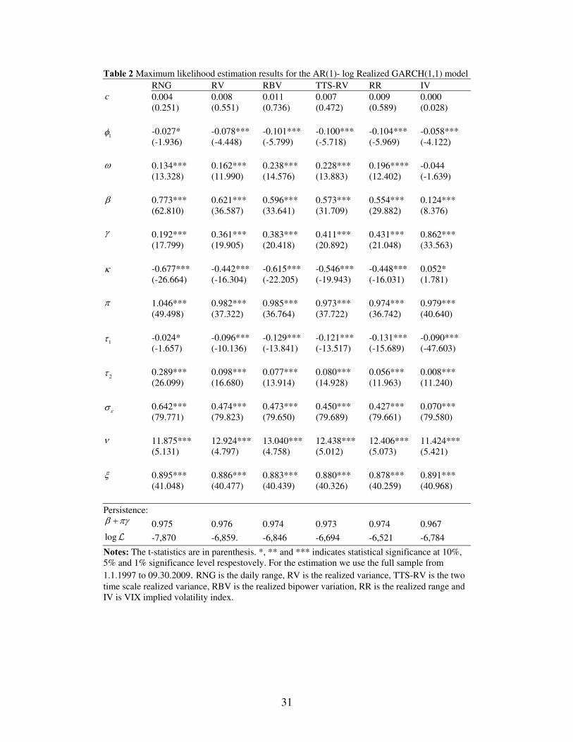
In Table 2, we present the Realized GARCH model maximum likelihood estimation results
for the full sample, i.e. from 1.1.1997 to 09.30.2009. Overall, almost all coefficients estimates
are statistically significant and their sign and magnitude are in accordance with the theoretical
assumptions and the previously reported estimation results of Hansen et al. (2011) and Watanabe
(2011). Starting form the conditional mean specification, we see that the autoregressive
parameter, 1φ̂ , is negative and statistically significant implying a negative autocorrelation in the
returns series. The skst distribution parameters estimates ˆˆ( , )ν ξ indicate fat tails and negative
skewness ( ˆ 1ξ < ) for the z’s density, while their estimates do not change significantly with use of
alternative volatility measures. The estimates of 1τ and 2τ in the measurement equation align
with the theory of leverage effects and volatility clustering.
Nonetheless, the most interesting results emerge from the estimation of κ and π parameters
in the measurement equation. Specifically, across volatility measures the estimates of π are
close to 1, ˆ 1π ≈ , which is an expected result since all volatility measures are ‘roughly’
proportional to the unobserved conditional variance (Hansen et al., 2011). However, for all
realized and range-based volatility measures the estimates of κ are much lower than zero
indicating that volatility estimators that utilize intraday data are biased. This result can be simply
explained from the fact that these measures are computed employing only the 6.5 active trading
hours (08:30-15:00 in our case) of day t, whereas the conditional variance, th , refers to a 24
hours time period which spans from the closing time (15:00) of day 1t − to the closing time
(15:00) of day t, since daily returns, tr , are calculated using close-to-close prices (see Hansen et
al., 2011 for a related discussion). Moreover, the RNG and the RBV estimators have the lowest
estimates of κ . One possible explanation is that the theoretical foundation of Parkison’s RNG
estimator is based on the restrictive assumption of zero drift geometric Brownian motion which
may result in biased estimates in real-world settings. Indeed, the authors in Alizadeh et al.
(2002), Brand and Diebold (2003) and Shu and Zang (2006), based on simulation results, find
evidence of downward bias for the RNG estimator. Furthermore, the RBV estimator is robust
against jumps implying that on average is lower or equal to the quadratic variation of the price

18
process as estimated by the RV (see section 3). Consequently, the κ estimates for the RBV are
expected to be lower compared to those of the RV estimator. On the contrary, when we use the
IV as a volatility proxy the estimation of κ is very close to zero ( ˆ 0.052κ = ) and marginally
statistically significant at a 10% significance level. This evidence indicates that the IV is almost
an unbiased estimator of the daily conditional volatility. From the GARCH equation results it is
also obvious that the IV measure has the greatest impact on future volatility ( ˆ 0.862γ = )
compared to its realized/range counterparts while the persistence is also high with the persistence
parameter being approximately 0.97 across volatility measures and very close to the estimation
results reported by Hansen et al. (2011).
In Figure 2, we illustrate the Monte Carlo simulated returns using the RR volatility estimator
for the last day of our sample i.e. 09/30/2009. The graph compares the simulated returns with the
normal density of equal variance. For all four forecasting horizons the simulated returns are
negatively skewed and possess fat tails relative to the normal density implying the
inappropriateness of Gaussian assumption for the VaR applications.
[Insert Table 2 about here]
[Insert Figure 2 about here]
5.2. VaR forecasting evaluation results
We use a rolling window of approximately five years or 1,250 trading days in order to
produce the out-of-sample VaR forecasts from 12.20.2000 to 09.30.2009.3 Table 3 presents the
FR and the p-values for the (un)conditional coverage tests for a 5% and 1% coverage level. We
follow Beltratti and Morana (2005) and we report the lowest p-value obtained by the h
(un)conditional coverage tests performed for each of the h subseries of exceptions. We reject the
null hypothesis at a 0.05 significance level if the tests produce a p-value lower than 0.05/h. For
instance, for the monthly forecasts, i.e. for h = 20, the null hypothesis of correct (un)conditional
coverage is rejected if the LR test generates p-value lower than 0.0025.
3 For this period we generate 1,946 daily, 1,941 weekly, 1936 biweekly and 1926 monthly out-of-sample VaR forecasts.
19
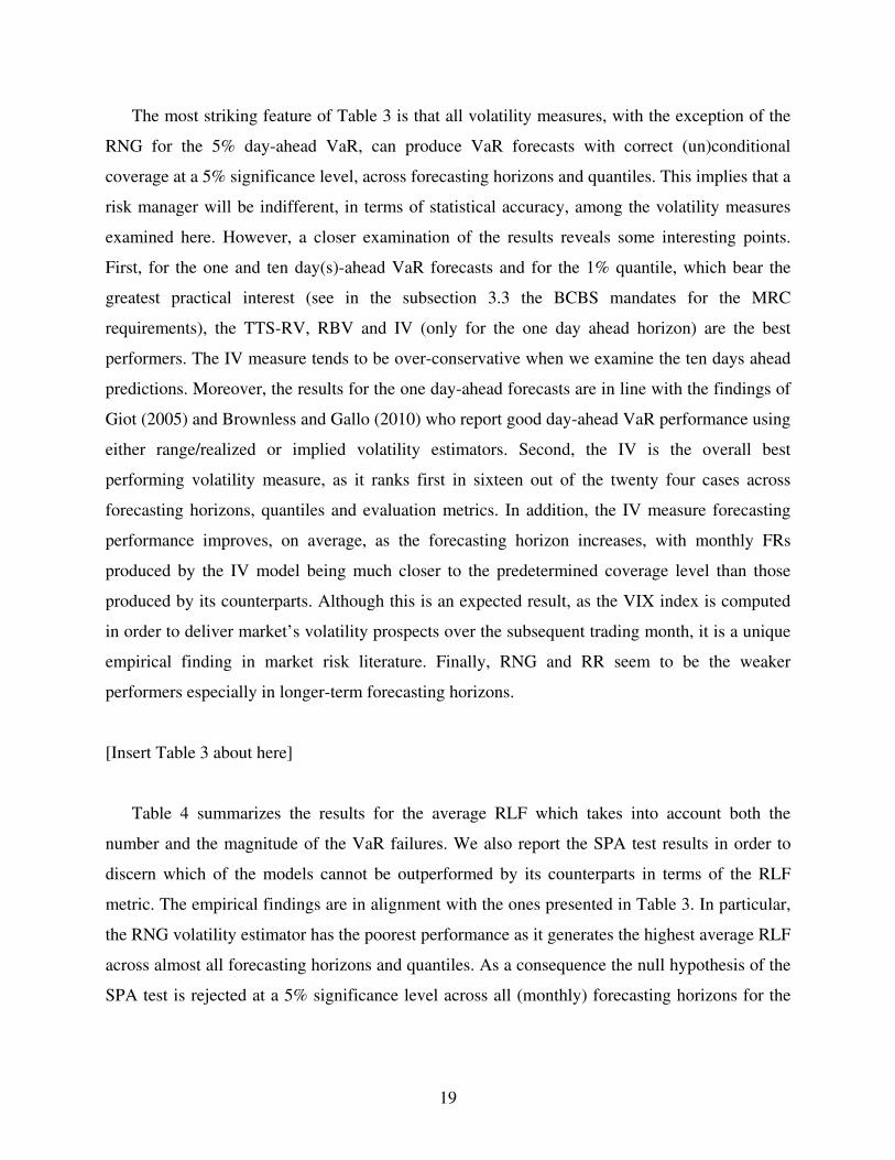
The most striking feature of Table 3 is that all volatility measures, with the exception of the
RNG for the 5% day-ahead VaR, can produce VaR forecasts with correct (un)conditional
coverage at a 5% significance level, across forecasting horizons and quantiles. This implies that a
risk manager will be indifferent, in terms of statistical accuracy, among the volatility measures
examined here. However, a closer examination of the results reveals some interesting points.
First, for the one and ten day(s)-ahead VaR forecasts and for the 1% quantile, which bear the
greatest practical interest (see in the subsection 3.3 the BCBS mandates for the MRC
requirements), the TTS-RV, RBV and IV (only for the one day ahead horizon) are the best
performers. The IV measure tends to be over-conservative when we examine the ten days ahead
predictions. Moreover, the results for the one day-ahead forecasts are in line with the findings of
Giot (2005) and Brownless and Gallo (2010) who report good day-ahead VaR performance using
either range/realized or implied volatility estimators. Second, the IV is the overall best
performing volatility measure, as it ranks first in sixteen out of the twenty four cases across
forecasting horizons, quantiles and evaluation metrics. In addition, the IV measure forecasting
performance improves, on average, as the forecasting horizon increases, with monthly FRs
produced by the IV model being much closer to the predetermined coverage level than those
produced by its counterparts. Although this is an expected result, as the VIX index is computed
in order to deliver market’s volatility prospects over the subsequent trading month, it is a unique
empirical finding in market risk literature. Finally, RNG and RR seem to be the weaker
performers especially in longer-term forecasting horizons.
[Insert Table 3 about here]
Table 4 summarizes the results for the average RLF which takes into account both the
number and the magnitude of the VaR failures. We also report the SPA test results in order to
discern which of the models cannot be outperformed by its counterparts in terms of the RLF
metric. The empirical findings are in alignment with the ones presented in Table 3. In particular,
the RNG volatility estimator has the poorest performance as it generates the highest average RLF
across almost all forecasting horizons and quantiles. As a consequence the null hypothesis of the
SPA test is rejected at a 5% significance level across all (monthly) forecasting horizons for the

20
5% (1%) quantile.4 On the other hand, IV model seems to have an adequate performance across
forecasting horizons as it does not reject the SPA test hypothesis, but for the 5% day-ahead VaR
predictions. The IV is again the best performing measure for the longest (monthly) forecasting
horizon since it minimizes the RLF for both coverage levels. With the exception of the RR and
the RBV for the 5% bi-weekly and monthly VaR forecasts respectively, in all other cases the
realized volatility measures behave quite well as they are not outperformed by any of their
counterparts. Nonetheless, the RV model has the most consistent behaviour as it ranks first for
the one, five and ten-days ahead forecasts irrespective of the quantile used.
[Insert Table 4 about here]
The picture is different regarding the efficiency of the VaR forecasts as measured by the
average FLF. The empirical findings, presented in Table 5, suggest that when we account for the
opportunity cost of capital, the IV and the RV measures are the worst performers. They generate
the overall highest average FLF and reject the SPA test hypothesis irrespective of the horizon
examined, with the only exception being the 5% day-ahead and monthly VaR forecasts for the
IV and the RV measure respectively. On the contrary, RNG, TTS-RV, RBV and RR models
produce the most efficient weekly, biweekly and monthly VaR forecasts as they are not
outperformed by any other volatility measure according to the SPA test results (the only
exception is the RR model for the 5% biweekly VaR forecasts). For the 5% and 1% day-ahead
VaR forecasts RR and RNG respectively are the only historical volatility measures that do not
reject the null hypothesis of the SPA test. A possible explanation is that these volatility
estimators are robust against either the microstructure noise bias or the price jumps and thus,
they can mitigate extreme or noisy price movements. Consequently, the models incorporating
these volatility measures produce moderate VaR estimates that help minimize the opportunity
cost of capital.
[Insert Table 5 about here]
4 In the spirit of Sarma et al. (2003) for the 5% quantile we do not include the RNG model in the SPA test as it does not pass the unconditional coverage tests (see Table 3)

21
The results for the MRC requirements, presented in Table 6, confirm the aforementioned
findings. The RNG volatility estimator is the worst performer in terms of regulatory accuracy as
it is the only volatility measure that produces red light days. All other volatility proxies comply
with the regulators accuracy rules. In terms of efficiency, the RR and RBV volatility measures
generate the lowest regulatory capital with the other two realized volatility estimators lagging
closely behind. The highest regulatory capital is generated by the IV measure indicating its
relative inefficiency. The SPA test results also confirm these findings. Figure 3 shows the market
risk capital requirements estimates for the six alternative volatility measures. The graph reveals
that the capital requirements increase considerably during the 2007-2009 crisis and that the IV
measure generates the highest regulatory capital reserves especially from 2003 to 2007 and after
the end of 2009.
[Insert Table 6 about here]
[Insert Figure 3 about here]
Table 7 summarizes the average performance of the alternative volatility measures across
forecasting horizons and quantiles. Overall, the best performing volatility measures are the RR
and the RBV as they manage to combine statistical accuracy, regulatory compliance and capital
efficiency, while the TTS-RV is also a good alternate. The IV measure behaves very well in
terms of accuracy (both statistical and regulatory), especially in long term forecasts, but it tends
to produce inefficient VaR estimates. The RV measure has similar behavior with the IV measure,
while the RNG volatility estimator demonstrates inferior forecasting performance.
[Insert Table 7 about here]
6. Conclusions
We complement and extend the previous VaR literature by examining the informational
content of daily range, realized variance, realized bipower variation, two time scale realized
variance, realized range and implied volatility in a multi-step VaR forecasting context. In our

22
analysis we use the recently proposed Realized GARCH model of Hansen et al. (2011) which
allows for the joint modelling of alternative volatility measures and returns. The Realized
GARCH model is combined with the skewed student distribution, which captures the fat tails
and the asymmetry of returns distribution, and a Monte Carlo simulation methodology for the
multi-step VaR forecasts.
Based on the S&P 500 stock index and on an approximately eight years of out-of-sample
forecasts, including the turbulent period 2007-2009, we find that almost all volatility measures
can produce statistically accurate multi-step VaR forecasts. The only exception is the daily range
for the 5% day-ahead VaR forecasts. Our empirical findings are in accordance with Giot (2005)
and indicate that the implied volatility measure is a good alternative volatility estimator for
market risk applications, especially for longer term (monthly) VaR predictions.
The results for a loss function that reflects regulators’ preferences are in alignment with the
statistical accuracy results. However, when we employ a loss function that considers the
opportunity cost of capital the results are slightly different. Now, daily range and high frequency
data volatility estimators that are robust against either the microstructure noise bias or the price
jumps generate the most efficient VaR estimates that minimize the opportunity cost of capital.
A real-world application based on Basel II regulatory framework confirms the above
mentioned findings. In particular, all volatility measures, except for the daily range, comply with
the regulators’ mandates regarding the number of exceptions during the previous trading year.
Moreover, the adjusted realized range (Martens and van Dijk, 2007) and the realized bipower
variation (Barndorff-Nielsen and Shephard, 2004), which are robust against microstructure noise
and price jumps respectively, minimize the market risk capital requirements and thus, the
released idle capital can be used in more efficient and productive ways.
Therefore, a risk manager or a regulator who emphasizes on statistical and regulatory
precision of the VaR estimates will be indifferent among the realized or the implied volatility
measures examined here and perhaps he will choose the implied volatility for the monthly
forecasting horizons. Nonetheless, a risk manager who is more concerned with efficiency issues,
without disregarding the importance of statistical accuracy and regulatory compliance, he will
concentrate on realized range and realized bipower variation measures.
Our empirical results give evidence in favour of robust high frequency intra-daily data
volatility estimators since they balance between statistical or regulatory accuracy and capital

23
efficiency. However, further research is required in order to gain more insights on the
informational content of alternative volatility measures in multi-period VaR forecasting using
other stock indices or asset classes such as stocks, bonds, currencies or commodities.

24
References
Alexander C. 2008a. Market Risk Analysis: Pricing, Hedging and Trading Financial
Instruments, vol III. Wiley: New York.
Alexander C. 2008b. Market Risk Analysis: Value-at-Risk Models, vol IV. Wiley: New York.
Alizadeh S, Brandt M, Diebold F. 2002. Range-based estimation of stochastic volatility models.
Journal of Finance 57: 1047-1091.
Andersen TG, Bollerslev T. 1998. Answering the skeptics: Yes, standard volatility models do
provide accurate forecasts. International Economic Review 39: 885-905.
Andersen TG, Bollerslev T, Diebold FX, Ebens H. 2001a. The distribution of realized stock
returns volatility. Journal of Financial Economics 6: 43-76.
Andersen TG, Bollerslev T, Diebold FX, Labys P. 2001b. The distribution of realized exchange
rate volatility. Journal of the American Statistical Association 96: 42-55.
Andersen TG, Bollerslev T, Diebold FX, Labys P. 2003. Modeling and forecasting realized
volatility. Econometrica 71: 579-625.
Andersen TG, Bollerslev T, Christoffersen PF, Diebold FX. 2006. Volatility and correlation
forecasting. In: Elliott, G., et al. (Eds.), Handbook of Economic Forecasting: Vol. I, North-
Holland.
Angelidis T, Degiannakis S. 2008. Volatility forecasting: Intra-day versus Inter-day models.
Journal of International Financial Markets, Institutions and Money 18: 449-465.
Angelidis T, Benos A, Degiannakis S. 2004. The use of GARCH models in VaR estimation.
Statisitcal Methodology 1: 105-128.
Barndorff-Nielsen OE, Shephard N. 2002. Econometric analysis of realized volatility and its use
in estimating stochastic volatility models. Journal of the Royal Statistical Society. B 64: 253-
280.
Barndorff-Nielsen OE, Shephard N. 2004. Power and bipower variation with stochastic volatility
and jumps. Journal of Financial Econometrics 2: 1-48.
Barndorff-Nielsen OE, Hansen PR, Lunde A,. Shephard N. 2008. Designing realized kernels to
measure the ex post variation of equity prices in the presence of noise. Econometrica
76: 1481-1536.
Basel Committee on Banking Supervision. 1996a. Amendment to the Capital Accord to
incorporate market risks. Bank for International Settlements: Basel.

25
Basle Committee on Banking Supervision 1996b. Supervisory framework for the use of
backtesting in conjunction with the internal models approach to market risk capital
requirements. Bank for International Settlements, Publication No. 22.
Basel Committee on Banking Supervision. 2006. International convergence of capital
measurement and capital standards. Bank for International Settlements: Basel.’
Becker R, Clements AE, McClelland A. 2009. The jump component of S&P 500 volatility and
the VIX index. Journal of Banking and Finance 33: 1033-1038.
Beltratti A., Morana C. 2005. Statistical Benefits of Value-at-risk with long memory. Journal of
Risk 7: 21-45.
Blair BJ, Poon S, Taylor SJ. 2001. Forecasting S&P 100 volatility: The incremental information
content of implied volatility and high frequency index returns. Journal of Econometrics 105:
5-26.
Bollerslev T. 1986. Generalized autoregressive heteroskedasticity. Journal of Econometrics 31:
307-327.
Bollerslev T. 2010. Glossary to ARCH (GARCH). In: Bollerslev, T., et al. (Eds.), Volatility and
time series econometrics: Essays in honor of Robert F. Engle. Oxford University Press.
Brandt MW, Diebold FX. 2003. A vp-arbitrage approach to range-based estimation of return
covariances and correlations. NBER Working Paper No. 9664.
Brooks C, Persand G. 2003. Volatility forecasting for risk management. Journal of forecasting
22: 1-22.
Brownless CT, Gallo GM. 2010. Comparison of volatility measures: A risk management
perspective. Journal of Financial Econometrics 8: 29-56.
Campel A., Chen XL. 2008. The year of living riskily. Risk July 2008: 28-32.
Chicago Board of Options Exchange. 2003. White Paper, VIX CBOE Volatility Index.
Accessible from: http://www.cboe.com/micro/vix/introduction.aspx.
Christensen PJ, Prabhala NR. 1998. The relation of between implied and realized volatility.
Journal of Financial Economics 50: 125-150.
Christensen K, Podolskij M. 2007. Realized range-based estimation of integrated variance.
Journal of Econometrics 141: 323-349.
Christoffersen P. 1998. Evaluating interval forecasts. International Economic Review 39: 841-
862.

26
Christoffersen PF. 2003. Elements of Financial Risk Management. Academic Press: San Diego.
Chou R. 2005. Forecasting financial volatilities with extreme values: The conditional
autoregressive range (CARR) model. Journal of Money Credit and Banking 37: 561-582.
Chou RY, Chou H, Liu N. 2010. Range volatility models and their applications in finance. ). In:
Lee C-F, et al. (Eds.), Handbook of Quantitative Finance and Risk Management. Springer.
Corrado C, Miller TW. 2005. The forecast quality of CBOE implied volatility indexes. Journal
of Futures Markets 25: 339-373.
Corrado C, Truong C. 2007. Forecasting stock index volatility: Comparing implied volatility and
the intraday high-low price range. The Journal of Financial Research XXX: 201-207.
Diebold FX, Gunther TA, Tay AS. 1998. Evaluating density forecasts. International Economic
Review 39: 863-883.
Drakos AA, Kouretas GP, Zarangas LP. 2010. Forecasting financial volatility of the Athens
stock exchange daily returns: An application of the asymmetric normal mixture GARCH
model. International Journal of Finance and Economics 15: 331-350.
Engle RF. 1982. Autoregressive conditional heteroskedasticity with estimates of the variance of
United Kingdom inflation. Econometrica 50: 987-1007.
Engle RF. 2002. New frontiers for ARCH models. Journal of Applied Econometrics 17: 425-
446.
Engle RF, Gallo JP. 2006. A multiple indicator model for volatility using intra daily data.
Journal of Econometrics 131: 3-27.
Fernandez C, Steel M. 1998. On Bayesian modeling of fat tails and skeweness. Journal of the
American Statistical Association 93: 359-371.
Ferreira MA., Lopez JA. 2005. Evaluating interest rate covariance models within a Value-at-Risk
framework. Journal of Financial Econometrics 3: 126-168.
Forsberg L, Ghysels E. 2007. Why do absolute returns predict volatility so well? Journal of
Financial Econometrics 5: 31-67.
Fuertes AM, Izzeldin M, Kalotychou E. 2009. On forecasting daily stock volatility: The role of
intraday information and market conditions. International Journal of Forecasting 25: 259-
281.
27
Garman M, Klass M. 1980. On the estimation of security price volatilities from historical data.
Journal of Business 53: 67-78.
Ghysels E, Sinko A.. 2006. Comment on Hansen and Lunde JBES paper. Journal of Business
and Economic Forecasting 26:192-194.
Ghysels E, Santa-Clara P, Valkanov R. 2006. Predicting volatility: How to get most out of
returns data sampled at different frequencies. Journal of Econometrics 131: 59-95.
Giot P, Laurent S. 2003a. Value-at-risk for long and short trading positions. Journal of Applied
Econometrics 6: 641-663.
Giot P, Laurent S. 2003b. Market risk in commodity markets: A VaR approach. Energy
Economics 25: 435-457.
Giot P, Laurent S. 2004. Modeling daily value-at-risk using realized volatility and ARCH type
models. Journal of Empirical Finance 11: 379-398.
Giot P, Laurent S. 2007. The information content of implied volatility in the light of
jump/continuous decomposition of realized volatility. The Journal of Future Markets 27:
337-359.
Giot P. 2005. Implied volatility indexes and daily Value at Risk models. The Journal of
derivatives 12: 54-64.
Hamilton JD. 1994. Time Series Analysis. Princeton University Press: Princeton.
Hansen PR. 2005. A test for superior predictive ability. Journal of Business and Economic
Statistics 23: 365-380.
Hansen PR, Huang Z, Shek HH. 2011. Realized GARCH: a joint model for returns and realized
measures of volatility. Journal of Applied Econometrics. doi: 10.1002/jae.1234.
Koopman SJ, Jungbacker B, Hol E. 2005. Forecasting daily variability of the S&P100 stock
index using historical, realised and implied volatility measurements. Journal of Empirical
Finance 12: 445-475.
Kuester K, Mittnik S, Paolella MS. 2006. Value-at-Risk prediction: A comparison of alternative
strategies. Journal of Financial Econometrics 4: 53-89.
Lambert P, Laurent S. 2001. Modelling financial time series using GARCH-type models and
skewed Student density. Mimeo, Universite de Liege.

28
Lawerence CT, Tits AL. 2001. A computationally efficient feasible sequential quadratic
programming algorithm. SIAM Journal on Optimization 11:1092-1118.
Li H, Hong H. 2011. Financial volatility forecasting with range-based autoregressive volatility
model. Financial Research Letters 8: 69-76.
Liu C, Maheu JM. 2009. Forecasting realized volatility: A Bayesian model-averaging approach.
Journal of Applied Econometrics 24: 709-733.
Lopez JA. 1999. Methods for evaluating Value-at-Risk estimates. Federal Reserve Bank of San
Francisco Economic Review 2: 3-17.
Louzis DP, Xanthopoulos-Sisinis S, Refenes AP. 2011. Are realized volatility models good
candidates for alternative Value-at-Risk prediction strategies? MPRA Working Paper.
Louzis DP, Xanthopoulos-Sisinis S, Refenes AP. 2012. Stock index realized volatility
forecasting in the presence of heterogeneous leverage effects and long range dependence in
the volatility of realized volatility. Applied Economics 44: 3533-3550.
Martens M. 2002. Measuring and forecasting S&P 500 index-futures volatility using high-
frequency data. Journal of Futures Markets 22: 497-518.
Martens M, van Dijk D. 2007. Measuring volatility with realized range. Journal of Econometrics
138: 181-207.
Martens M, van Dijk D, Pooter M. 2009. Forecasting S&P 500 volatility: Long memory, level
shifts, leverage effects, day of the week seasonality and macroeconomic announcements.
International Journal of Forecasting 25: 282-303.
Parkison M. 1980. The extreme value method for estimating the variance of the rate of return.
Journal of Business. 53: 61-65.
Poon S, Granger C. 2003. Forecasting volatility in financial markets: A review. Journal of
Economic Literature 41: 478-539.
Rogers L, Satchell S. 1991. Estimating variance from high, low and closing prices. Annals of
Applied Probability 1: 504-512.
Sajjad R, Coakley J, Nankervis JC. 2008. Markov-Switching GARCH modeling of Value-at-
Risk. Studies in Nonlinear dynamics and Econometrics 12: Article 7.
Sarma M, Thomas S, Shah A. 2003. Selection of Value-at-Risk models. Journal of Forecasting
22: 337-358.
29
Shao XD, Lian YJ, Yin LQ, 2009. Forecasting Value-at-Risk using high frequency data: The
realized range model. Global Finance Journal 20, 128-136.
Shu JH, Zhang JE. 2006. Testing range estimators of historical volatility. Journal of Future
Markets 26: 297-313.
Watanabe T. 2011. Quintile forecasts of financial returns using Realized GARCH models. Hi-
Stat Discussion Paper, Hitotsubashi University.
Zhang L, Mykland PA, Aït-Sahalia Y. 2005. A tale of two time scales: Determining integrated
volatility with noisy high-frequency data. Journal of the American Statistical Association
100: 1394-1411.

30
Table 1 Distributional properties of daily returns and alternative volatility measures of the S&P 500 stock index
Mean St.Dev Skewness Kurtosis Max Min
Daily returns (%) 0.011 1.344 -0.089 6.770 10.714 -9.789
RNG 1.277 2.769 8.153 88.455 42.807 0.021
RV 1.335 2.718 10.857 208.011 75.364 0.053
RBV 1.128 2.288 9.337 133.231 51.707 0.047
TTS-RV 1.181 2.531 14.940 396.058 84.474 0.049
RR 1.286 2.612 11.394 215.305 71.759 0.058
IV 1.623 1.619 4.160 25.068 17.913 0.268
Notes: RNG is the daily range, RV is the realized variance, TTS-RV is the two time scale realized variance, RBV is the realized bipower variation, RR is the realized range and IV is VIX implied volatility index.
31
Table 2 Maximum likelihood estimation results for the AR(1)- log Realized GARCH(1,1) model
RNG RV RBV TTS-RV RR IV c 0.004
(0.251) 0.008 (0.551)
0.011 (0.736)
0.007 (0.472)
0.009 (0.589)
0.000 (0.028)
1φ -0.027* (-1.936)
-0.078*** (-4.448)
-0.101*** (-5.799)
-0.100*** (-5.718)
-0.104*** (-5.969)
-0.058*** (-4.122)
ω 0.134*** (13.328)
0.162*** (11.990)
0.238*** (14.576)
0.228*** (13.883)
0.196**** (12.402)
-0.044 (-1.639)
β 0.773*** (62.810)
0.621*** (36.587)
0.596*** (33.641)
0.573*** (31.709)
0.554*** (29.882)
0.124*** (8.376)
γ 0.192*** (17.799)
0.361*** (19.905)
0.383*** (20.418)
0.411*** (20.892)
0.431*** (21.048)
0.862*** (33.563)
κ -0.677*** (-26.664)
-0.442*** (-16.304)
-0.615*** (-22.205)
-0.546*** (-19.943)
-0.448*** (-16.031)
0.052* (1.781)
π 1.046*** (49.498)
0.982*** (37.322)
0.985*** (36.764)
0.973*** (37.722)
0.974*** (36.742)
0.979*** (40.640)
1τ -0.024* (-1.657)
-0.096*** (-10.136)
-0.129*** (-13.841)
-0.121*** (-13.517)
-0.131*** (-15.689)
-0.090*** (-47.603)
2τ 0.289*** (26.099)
0.098*** (16.680)
0.077*** (13.914)
0.080*** (14.928)
0.056*** (11.963)
0.008*** (11.240)
εσ 0.642*** (79.771)
0.474*** (79.823)
0.473*** (79.650)
0.450*** (79.689)
0.427*** (79.661)
0.070*** (79.580)
ν 11.875*** (5.131)
12.924*** (4.797)
13.040*** (4.758)
12.438*** (5.012)
12.406*** (5.073)
11.424*** (5.421)
ξ 0.895*** (41.048)
0.886*** (40.477)
0.883*** (40.439)
0.880*** (40.326)
0.878*** (40.259)
0.891*** (40.968)
Persistence: β πγ+ 0.975 0.976 0.974 0.973 0.974 0.967
logL -7,870 -6,859. -6,846 -6,694 -6,521 -6,784
Notes: The t-statistics are in parenthesis. *, ** and *** indicates statistical significance at 10%, 5% and 1% significance level respestovely. For the estimation we use the full sample from
1.1.1997 to 09.30.2009. RNG is the daily range, RV is the realized variance, TTS-RV is the two
time scale realized variance, RBV is the realized bipower variation, RR is the realized range and IV is VIX implied volatility index.

32
Table 3 Failure rates and Christoffersen’s (un)conditional coverage tests results
5% Coverage level
Volatility Daily (h = 1) Weekly (h = 5) Bi-weekly (h = 10) Monthly (h = 20)
measures FR(%) UC CC FR(%) UC CC FR(%) UC CC FR(%) UC CC
RNG 6.22 0.017 0.058 5.92 0.096 0.190 5.66 0.177 0.134 7.16 0.078 0.196
RV 4.98* 0.975* 0.996 5.77 0.096 0.190 4.12 0.089 0.206 7.21 0.035 0.100
TTS-RV 5.09 0.860 0.894 6.08 0.096 0.190 4.27 0.089 0.206 7.36 0.078 0.100
RBV 5.04 0.942 0.997* 6.13 0.061 0.122 4.07 0.196 0.358* 7.31 0.078 0.123
RR 5.19 0.702 0.877 5.82 0.096 0.190 5.36* 0.292* 0.224 7.16 0.035 0.107
IV 5.65 0.195 0.232 4.84* 0.114* 0.214* 3.45 0.034 0.097 5.97* 0.170* 0.125*
1% Coverage level
RNG 1.13 0.571 0.662 1.49 0.153 0.120 1.65 0.018 0.051 1.96 0.020 0.041*
RV 0.82 0.416 0.629 1.44 0.153 0.316* 0.77 0.455* 0.738* 2.16 0.020 0.041*
TTS-RV 0.98* 0.916* 0.402 1.49 0.066 0.117 0.98* 0.455* 0.738* 2.27 0.003 0.007
RBV 1.03 0.903 0.437 1.54 0.066 0.156 0.93 0.455* 0.742* 2.42 0.003 0.007
RR 0.82 0.416 0.629 1.65 0.066 0.120 1.80 0.018 0.051 2.37 0.003 0.007
IV 0.98* 0.916* 0.825* 1.08* 0.317* 0.083 0.72 0.455* 0.738* 1.65* 0.094* 0.041*
Notes: All forecasts are generated by the Realized GARCH model. RNG is the daily range, RV is the realized variance, TTS-RV is the two time scale realized variance, RBV is the realized bipower variation, RR is the realized range and IV is VIX implied volatility index. FR denotes the failure rate in percentage points, UC and CC are the p-values for the Christoffersen’s unconditional and conditional coverage tests respectively. The bold faced figures indicate rejection of the null at 0.05/h significance level. The table reports the lowest p-value across the h sub-series of exceptions. The asterisk (*) indicates the best performing model i.e. the model with the closest FR to the prespecified coverage level (α) and the highest p-value.

33
Table 4 Average regulatory loss function (RLF) and superior predictive Ability (SPA) test results
5% Coverage level
Volatility Daily (h = 1) Weekly (h = 5) Bi-weekly (h = 10) Monthly (h = 20)
measures RLF SPA-test RLF SPA-test RLF SPA-test RLF SPA-test
RNG 0.116 - 0.444 0.046 1.143 0.024 2.865 0.013
RV 0.082* 0.783* 0.383* 0.958* 0.658* 0.960* 2.492 0.325
TTS-RV 0.084 0.320 0.415 0.051 0.704 0.116 2.578 0.063
RBV 0.082 0.646 0.400 0.118 0.671 0.498 2.595 0.010
RR 0.084 0.284 0.391 0.493 1.089 0.009 2.609 0.104
IV 0.117 0.013 0.426 0.184 0.726 0.173 2.321* 0.858*
1% Coverage level
RNG 0.019 0.066 0.082 0.141 0.405 0.100 1.152 0.049
RV 0.013* 0.974* 0.068* 0.977* 0.178* 0.917* 0.806 0.645
TTS-RV 0.015 0.232 0.076 0.115 0.195 0.314 0.816 0.602
RBV 0.015 0.226 0.068 0.311 0.178 0.803 0.810 0.734
RR 0.013 0.651 0.065 0.116 0.382 0.055 0.822 0.512
IV 0.018 0.168 0.126 0.132 0.244 0.087 0.744* 0.836*
Notes: All forecasts are generated by the Realized GARCH model. RNG is the daily range, RV is the realized variance, TTS-RV is the two time scale realized variance, RBV is the realized bipower variation, RR is the realized range and IV is VIX implied volatility index. For the SPA test we show the p-values. The bold faced figures indicate rejection of the null at a 0.05 significance level. The asterisk indicates the best performing model i.e. the model with the lowest RLF and the highest SPA p-value.

34
Table 5 Average firm loss function (FLF) and superior predictive Ability (SPA) test results
5% Coverage level
Volatility Daily (h = 1) Weekly (h = 5) Bi-weekly (h = 10) Monthly (h = 20)
measures FLF SPA-test FLF SPA-test FLF SPA-test FLF SPA-test
RNG 2.684 - 5.965 0.346 8.825 0.072 13.499 0.141
RV 2.829 0.006 6.024 0.000 8.591 0.001 13.364 0.072
TTS-RV 2.818 0.022 5.948 0.424 8.481* 0.725* 13.278* 0.957*
RBV 2.821 0.030 5.933 0.802 8.499 0.473 13.300 0.690
RR 2.818 0.052 5.932* 0.803* 8.837 0.028 13.289 0.795
IV 2.745* 0.571* 6.315 0.000 9.242 0.000 14.391 0.000
1% Coverage level
RNG 4.178* 0.616* 8.800* 0.615 12.509 0.373 17.943 0.080
RV 4.380 0.000 8.913 0.000 12.534 0.000 17.864 0.000
TTS-RV 4.371 0.000 8.832 0.150 12.405 0.510 17.726 0.106
RBV 4.364 0.000 8.803 0.794* 12.381* 0.924* 17.666 0.771
RR 4.375 0.001 8.806 0.695 12.526 0.252 17.658* 0.858*
IV 4.437 0.000 9.484 0.000 13.714 0.000 20.276 0.000
Notes: All forecasts are generated by the Realized GARCH model. RNG is the daily range, RV is the realized variance, TTS-RV is the two time scale realized variance, RBV is the realized bipower variation, RR is the realized range and IV is VIX implied volatility index. For the SPA test we show the p-vlaues. The bold faced figures indicate rejection of the null at a 0.05 significance level. The asterisk indicates the best performing model i.e. the model with the lowest FLF and the highest SPA p-value.

35
Table 6 Basel II market risk capital requirements
Volatility Basel II zones Basel II Capital requirements
measures Green (%) Yellow (%) Red (%) Mean SPA test
RNG 69.104 28.597 2.300
268.800 -
RV 81.250 18.750 0.000
263.968 0.000
TTS-RV 75.531 24.469 0.000
265.351 0.000
RBV 80.483 19.517 0.000
263.412* 0.515*
RR 75.531 24.469 0.000
263.567 0.479
IV 84.375 15.625 0.000
294.383 0.000
Notes: RNG is the daily range, RV is the realized variance, TTS-RV is the two time scale realized variance, RBV is the realized bipower variation, RR is the realized range and IV is the VIX implied volatility index. The table presents the percentage of days during the out of sample forecasting period that the model is placed in the green, yellow and red zone according to the Basel traffic light system, the average daily capital requirements and Superior Predictive Ability (SPA) test p-values. The bold faced figures indicate rejection of the null at a 0.05 significance level.

36
Table 7 Summary of the empirical results
Basel II market risk regulatory capital
Volatility measures
Statistical Accuracy (Coverage tests)
Regulatory Accuracy (RLF)
Capital Efficiency (FLF)
Accuracy (Number of exceptions during
the previous trading year)
Efficiency (Minimization of the regulatory capital)
RNG Yes No Yes No No
RV Yes Yes No Yes No
TTS-RV Yes Yes Yes Yes No
RBV Yes Yes Yes Yes Yes
RR Yes Yes Yes Yes Yes
IV Yes Yes No Yes No
Notes: RNG is the daily range, RV is the realized variance, TTS-RV is the two time scale realized variance, RBV is the realized bipower variation, RR is the realized range and IV is the VIX implied volatility index. The table shows the average performance of the volatility measures across forecasting horizons and quantiles. A volatility measure is considered as inadequate (No) if it fails in 4 or more out of the total 8 forecasting schemes examined here, i.e. 4 forecasting horizons and 2 quantiles. For the Basel II market risk regulatory capital the results are based solely on Table 6.

37

38

39