the role of knowledge extraction in computer go
TRANSCRIPT

The Role of Knowledge Extraction in Computer Go
Simon Viennot
Japan Advanced Institute of Science and Technology
December 15th, 2014

Japan, Kanazawa
Japan
Kanazawa, Sea of Japan
Snow during winter

Japan, Kanazawa
Japan
Kanazawa, Sea of Japan
Snow during winter

Japan, Kanazawa
Japan
Kanazawa, Sea of Japan
Snow during winter

JAIST
Japan Advanced Institute of Science and Technology (JAIST)
Master and doctor courses
Information ScienceKnowledge ScienceMaterial Science
Information Science > Artificial Intelligence > GamesAssistant professor (since 2013)

JAIST
Japan Advanced Institute of Science and Technology (JAIST)
Master and doctor courses
Information ScienceKnowledge ScienceMaterial Science
Information Science > Artificial Intelligence > GamesAssistant professor (since 2013)

JAIST
Japan Advanced Institute of Science and Technology (JAIST)
Master and doctor courses
Information ScienceKnowledge ScienceMaterial Science
Information Science > Artificial Intelligence > GamesAssistant professor (since 2013)

Past and current work
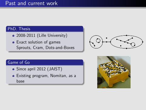
PhD. Thesis
2008-2011 (Lille University)
Exact solution of gamesSprouts, Cram, Dots-and-Boxes
Game of Go
Since april 2012 (JAIST)
Existing program, Nomitan, as abase
Past and current work
PhD. Thesis
2008-2011 (Lille University)
Exact solution of gamesSprouts, Cram, Dots-and-Boxes
Game of Go
Since april 2012 (JAIST)
Existing program, Nomitan, as abase

Section 1
Game of Go

The success of Computer Chess
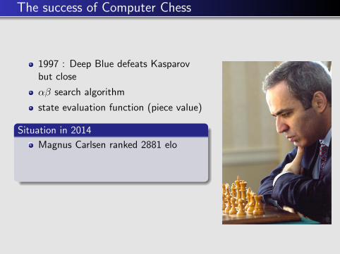
1997 : Deep Blue defeats Kasparovbut close
αβ search algorithm
state evaluation function (piece value)
Situation in 2014
Magnus Carlsen ranked 2881 elo
Top program ranked 3270 eloon a standard 4-core pc (Houdini)
⇒ Winning probability = 91%

The success of Computer Chess
1997 : Deep Blue defeats Kasparovbut close
αβ search algorithm
state evaluation function (piece value)
Situation in 2014
Magnus Carlsen ranked 2881 elo
Top program ranked 3270 eloon a standard 4-core pc (Houdini)
⇒ Winning probability = 91%

The success of Computer Chess
1997 : Deep Blue defeats Kasparovbut close
αβ search algorithm
state evaluation function (piece value)
Situation in 2014
Magnus Carlsen ranked 2881 elo
Top program ranked 3270 eloon a standard 4-core pc (Houdini)
⇒ Winning probability = 91%

The success of Computer Chess
1997 : Deep Blue defeats Kasparovbut close
αβ search algorithm
state evaluation function (piece value)
Situation in 2014
Magnus Carlsen ranked 2881 elo
Top program ranked 3270 eloon a standard 4-core pc (Houdini)
⇒ Winning probability = 91%
The success of Computer Chess
1997 : Deep Blue defeats Kasparovbut close
αβ search algorithm
state evaluation function (piece value)
Situation in 2014
Magnus Carlsen ranked 2881 elo
Top program ranked 3270 eloon a standard 4-core pc (Houdini)
⇒ Winning probability = 91%

The success of Computer Chess
1997 : Deep Blue defeats Kasparovbut close
αβ search algorithm
state evaluation function (piece value)
Situation in 2014
Magnus Carlsen ranked 2881 elo
Top program ranked 3270 eloon a standard 4-core pc (Houdini)
⇒ Winning probability = 91%

The success of Computer Chess
1997 : Deep Blue defeats Kasparovbut close
αβ search algorithm
state evaluation function (piece value)
Situation in 2014
Magnus Carlsen ranked 2881 elo
Top program ranked 3270 eloon a standard 4-core pc (Houdini)
⇒ Winning probability = 91%

Comparison of Chess and Go
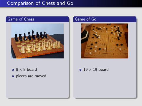
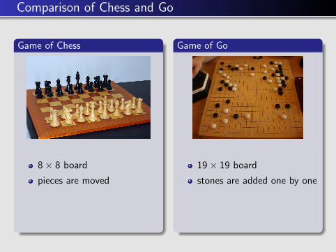
Game of Chess
8× 8 board
pieces are moved
300-500 (India)
600 millions players(spread worldwide)
Game of Go
19× 19 board
stones are added one by one
400 BC (China)
60 millions players(China, Japan, Korea)

Comparison of Chess and Go
Game of Chess
8× 8 board
pieces are moved
300-500 (India)
600 millions players(spread worldwide)
Game of Go
19× 19 board
stones are added one by one
400 BC (China)
60 millions players(China, Japan, Korea)

Comparison of Chess and Go
Game of Chess
8× 8 board
pieces are moved
300-500 (India)
600 millions players(spread worldwide)
Game of Go
19× 19 board
stones are added one by one
400 BC (China)
60 millions players(China, Japan, Korea)

Comparison of Chess and Go
Game of Chess
8× 8 board
pieces are moved
300-500 (India)
600 millions players(spread worldwide)
Game of Go
19× 19 board
stones are added one by one
400 BC (China)
60 millions players(China, Japan, Korea)
Comparison of Chess and Go
Game of Chess
8× 8 board
pieces are moved
300-500 (India)
600 millions players(spread worldwide)
Game of Go
19× 19 board
stones are added one by one
400 BC (China)
60 millions players(China, Japan, Korea)
Comparison of Chess and Go
Game of Chess
8× 8 board
pieces are moved
300-500 (India)
600 millions players(spread worldwide)
Game of Go
19× 19 board
stones are added one by one
400 BC (China)
60 millions players(China, Japan, Korea)

Comparison of Chess and Go
Game of Chess
8× 8 board
pieces are moved
300-500 (India)
600 millions players(spread worldwide)
Game of Go
19× 19 board
stones are added one by one
400 BC (China)
60 millions players(China, Japan, Korea)

Comparison of Chess and Go
Game of Chess
8× 8 board
pieces are moved
300-500 (India)
600 millions players(spread worldwide)
Game of Go
19× 19 board
stones are added one by one
400 BC (China)
60 millions players(China, Japan, Korea)

Comparison of Chess and Go
Game of Chess
8× 8 board
pieces are moved
300-500 (India)
600 millions players(spread worldwide)
Game of Go
19× 19 board
stones are added one by one
400 BC (China)
60 millions players(China, Japan, Korea)

Comparison of Chess and Go
Game of Chess
8× 8 board
pieces are moved
300-500 (India)
600 millions players(spread worldwide)
Game of Go
19× 19 board
stones are added one by one
400 BC (China)
60 millions players(China, Japan, Korea)

Rules of the game of Go
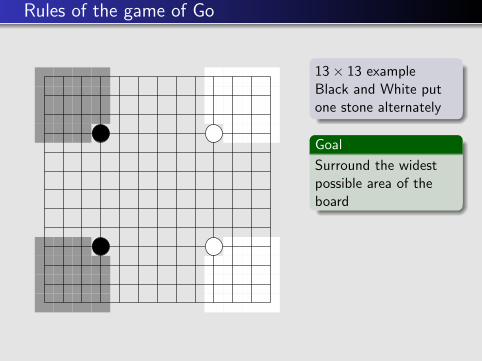
13× 13 exampleBlack and White putone stone alternately
Goal
Surround the widestpossible area of theboard
End of the game
25 Black points
26 White points
⇒ White wins

Rules of the game of Go
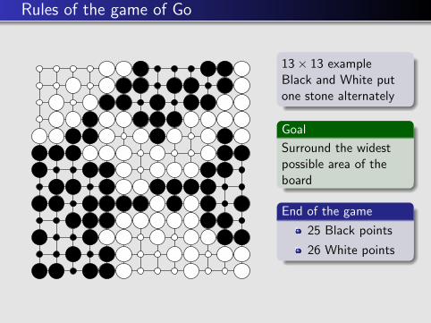
13× 13 exampleBlack and White putone stone alternately
Goal
Surround the widestpossible area of theboard
End of the game
25 Black points
26 White points
⇒ White wins

Rules of the game of Go
13× 13 exampleBlack and White putone stone alternately
Goal
Surround the widestpossible area of theboard
End of the game
25 Black points
26 White points
⇒ White wins

Rules of the game of Go
13× 13 exampleBlack and White putone stone alternately
Goal
Surround the widestpossible area of theboard
End of the game
25 Black points
26 White points
⇒ White wins
Rules of the game of Go
13× 13 exampleBlack and White putone stone alternately
Goal
Surround the widestpossible area of theboard
End of the game
25 Black points
26 White points
⇒ White wins

Rules of the game of Go
13× 13 exampleBlack and White putone stone alternately
Goal
Surround the widestpossible area of theboard
End of the game
25 Black points
26 White points
⇒ White wins

Rules of the game of Go
13× 13 exampleBlack and White putone stone alternately
Goal
Surround the widestpossible area of theboard
End of the game
25 Black points
26 White points
⇒ White wins

Rules of the game of Go
13× 13 exampleBlack and White putone stone alternately
Goal
Surround the widestpossible area of theboard
End of the game
25 Black points
26 White points
⇒ White wins

Rules of the game of Go
13× 13 exampleBlack and White putone stone alternately
Goal
Surround the widestpossible area of theboard
End of the game
25 Black points
26 White points
⇒ White wins
Rules of the game of Go
13× 13 exampleBlack and White putone stone alternately
Goal
Surround the widestpossible area of theboard
End of the game
25 Black points
26 White points
⇒ White wins

Rules of the game of Go
13× 13 exampleBlack and White putone stone alternately
Goal
Surround the widestpossible area of theboard
End of the game
25 Black points
26 White points
⇒ White wins
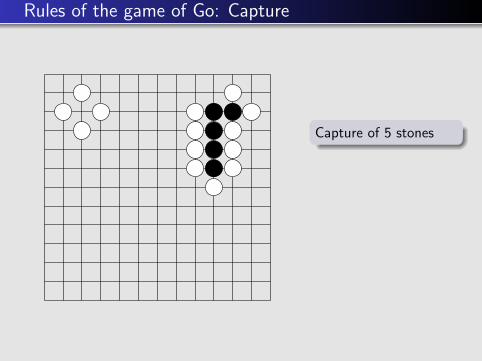
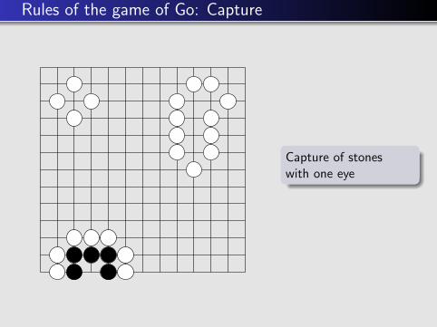
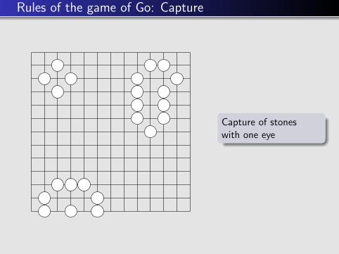
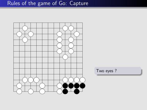
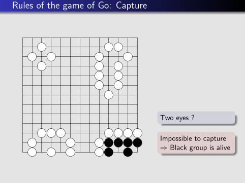
Rules of the game of Go: Capture
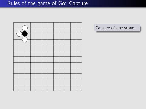
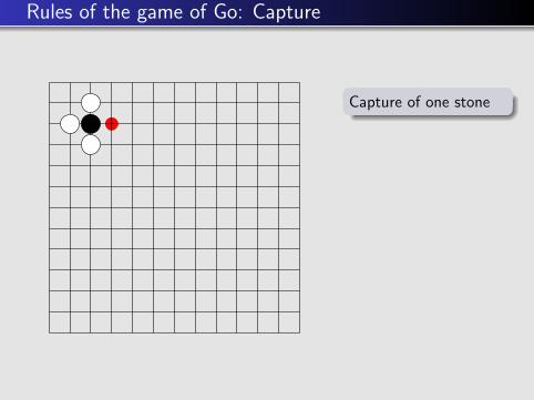
Capture of one stone
Capture of 5 stones
Capture of stoneswith one eye
Two eyes ?
Impossible to capture⇒ Black group is alive
Rules of the game of Go: Capture
Capture of one stone
Capture of 5 stones
Capture of stoneswith one eye
Two eyes ?
Impossible to capture⇒ Black group is alive

Rules of the game of Go: Capture
Capture of one stone
Capture of 5 stones
Capture of stoneswith one eye
Two eyes ?
Impossible to capture⇒ Black group is alive
Rules of the game of Go: Capture
Capture of one stone
Capture of 5 stones
Capture of stoneswith one eye
Two eyes ?
Impossible to capture⇒ Black group is alive

Rules of the game of Go: Capture
Capture of one stone
Capture of 5 stones
Capture of stoneswith one eye
Two eyes ?
Impossible to capture⇒ Black group is alive

Rules of the game of Go: Capture
Capture of one stone
Capture of 5 stones
Capture of stoneswith one eye
Two eyes ?
Impossible to capture⇒ Black group is alive
Rules of the game of Go: Capture
Capture of one stone
Capture of 5 stones
Capture of stoneswith one eye
Two eyes ?
Impossible to capture⇒ Black group is alive

Rules of the game of Go: Capture
Capture of one stone
Capture of 5 stones
Capture of stoneswith one eye
Two eyes ?
Impossible to capture⇒ Black group is alive
Rules of the game of Go: Capture
Capture of one stone
Capture of 5 stones
Capture of stoneswith one eye
Two eyes ?
Impossible to capture⇒ Black group is alive
Rules of the game of Go: Capture
Capture of one stone
Capture of 5 stones
Capture of stoneswith one eye
Two eyes ?
Impossible to capture⇒ Black group is alive
Rules of the game of Go: Capture
Capture of one stone
Capture of 5 stones
Capture of stoneswith one eye
Two eyes ?
Impossible to capture⇒ Black group is alive
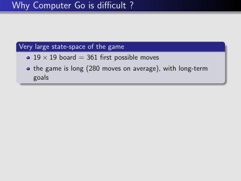
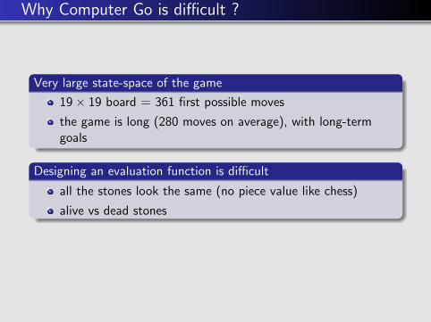
Why Computer Go is difficult ?
Very large state-space of the game
19× 19 board = 361 first possible moves
the game is long (280 moves on average), with long-termgoals
Designing an evaluation function is difficult
all the stones look the same (no piece value like chess)
alive vs dead stones
⇒ αβ search does not work well
Section 2
Current level
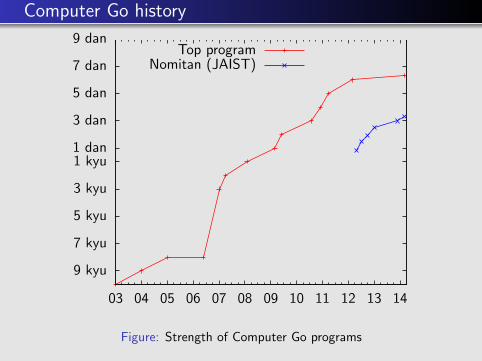
Computer Go history
9 kyu
7 kyu
5 kyu
3 kyu
1 kyu1 dan
3 dan
5 dan
7 dan
9 dan
03 04 05 06 07 08 09 10 11 12 13 14
Top programNomitan (JAIST)
Figure: Strength of Computer Go programs

UEC-cup competition
UEC-cup
University of Electro-Communications (Tokyo)
Currently biggest Computer Go competition
around 20 participants each year

UEC-cup 2013, 2014
Rank 2013 2014
1 Crazy Stone ≈ 6d Zen ≈ 6d
2 Zen ≈ 6d Crazy Stone ≈ 6d
3 Aya ≈ 4d Aya ≈ 4d
4 Pachi ≈ 2d Hirabot ≈ 2d
5 MP-Fuego ? Nomitan ≈ 3d
6 Nomitan ≈ 2d Gogataki < 1d
7 The Many Faces of Go ≈ 3d LeafQuest < 1d
2012 2013 2014
Nomitan rank 13th 6th 5th

Computer power
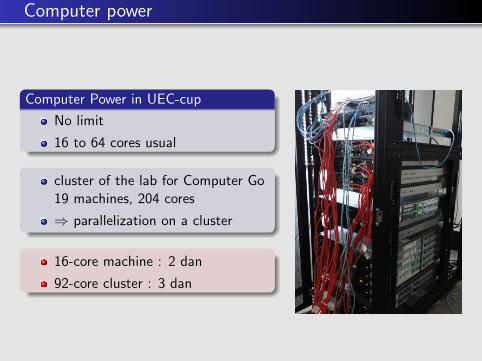
Computer Power in UEC-cup
No limit
16 to 64 cores usual
cluster of the lab for Computer Go19 machines, 204 cores
⇒ parallelization on a cluster
16-core machine : 2 dan
92-core cluster : 3 dan

Computer power
Computer Power in UEC-cup
No limit
16 to 64 cores usual
cluster of the lab for Computer Go19 machines, 204 cores
⇒ parallelization on a cluster
16-core machine : 2 dan
92-core cluster : 3 dan
Computer power
Computer Power in UEC-cup
No limit
16 to 64 cores usual
cluster of the lab for Computer Go19 machines, 204 cores
⇒ parallelization on a cluster
16-core machine : 2 dan
92-core cluster : 3 dan

Section 3
Monte-Carlo Tree Search

Monte-Carlo Tree Search Breakthrough
SelectionTree policy
Expansion
SimulationSimulation policy
Backpropagation

Monte-Carlo Tree Search Breakthrough
SelectionTree policy
Expansion
SimulationSimulation policy
Backpropagation

Monte-Carlo Tree Search Breakthrough
SelectionTree policy
Expansion
SimulationSimulation policy
Backpropagation

Monte-Carlo Tree Search Breakthrough
SelectionTree policy
Expansion
SimulationSimulation policy
Backpropagation

Monte-Carlo Tree Search Breakthrough
SelectionTree policy
Expansion
SimulationSimulation policy
Backpropagation

Monte-Carlo Tree Search Breakthrough
Win/Loss
SelectionTree policy
Expansion
SimulationSimulation policy
Backpropagation

Monte-Carlo Tree Search Breakthrough
Win/Loss
SelectionTree policy
Expansion
SimulationSimulation policy
Backpropagation

Monte-Carlo Tree Search Breakthrough
Win/Loss
SelectionTree policy
Expansion
SimulationSimulation policy
Backpropagation

Monte-Carlo Tree Search Breakthrough
Win/Loss
SelectionTree policy
Expansion
SimulationSimulation policy
Backpropagation

Monte-Carlo Tree Search Breakthrough
Win/Loss
SelectionTree policy
Expansion
SimulationSimulation policy
Backpropagation

Upper Confidence Tree: Definition
For which candidate move should we run the next simulation ?
2002 Auer et al : Upper Confidence Bound (UCB) formula
2006, Kocsis, Szepesvari : UCB formula as the tree policy
wi number of wins of the node
ni number of visits of the node
n number of visits of the parentnode
UCB formula:
µi =wi
ni+ C ·
√ln n
ni
At each step of the selection step in Monte-Carlo Tree Search,choose the node that maximizes µi

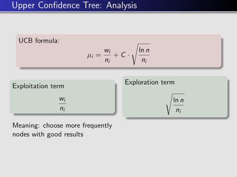
Upper Confidence Tree: Analysis
UCB formula:
µi =wi
ni+ C ·
√ln n
ni
Exploitation term
wi
ni
Exploration term√ln n
ni
Meaning: choose more frequentlynodes with good results
Meaning: choose more frequentlynodes not well explored
C is a parameter to balance the two terms

Upper Confidence Tree: Analysis
UCB formula:
µi =wi
ni+ C ·
√ln n
ni
Exploitation term
wi
ni
Exploration term√ln n
ni
Meaning: choose more frequentlynodes with good results
Meaning: choose more frequentlynodes not well explored
C is a parameter to balance the two terms

Upper Confidence Tree: Analysis
UCB formula:
µi =wi
ni+ C ·
√ln n
ni
Exploitation term
wi
ni
Exploration term√ln n
ni
Meaning: choose more frequentlynodes with good results
Meaning: choose more frequentlynodes not well explored
C is a parameter to balance the two terms
Upper Confidence Tree: Analysis
UCB formula:
µi =wi
ni+ C ·
√ln n
ni
Exploitation term
wi
ni
Exploration term√ln n
ni
Meaning: choose more frequentlynodes with good results
Meaning: choose more frequentlynodes not well explored
C is a parameter to balance the two terms

Upper Confidence Tree: Analysis
UCB formula:
µi =wi
ni+ C ·
√ln n
ni
Exploitation term
wi
ni
Exploration term√ln n
ni
Meaning: choose more frequentlynodes with good results
Meaning: choose more frequentlynodes not well explored
C is a parameter to balance the two terms

Upper Confidence Tree: Analysis
UCB formula:
µi =wi
ni+ C ·
√ln n
ni
Exploitation term
wi
ni
Exploration term√ln n
ni
Meaning: choose more frequentlynodes with good results
Meaning: choose more frequentlynodes not well explored
C is a parameter to balance the two terms

Asymmetric Tree Growth
Asymmetric growth of the tree developed by MCTS(Finnsonn PhD Thesis, 2012)

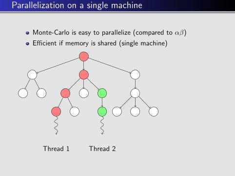
Parallelization on a single machine
Monte-Carlo is easy to parallelize (compared to αβ)
Efficient if memory is shared (single machine)
Thread 1
Parallelization on a single machine
Monte-Carlo is easy to parallelize (compared to αβ)
Efficient if memory is shared (single machine)
Thread 1 Thread 2

Parallelization on a single machine
Monte-Carlo is easy to parallelize (compared to αβ)
Efficient if memory is shared (single machine)
Thread 1 Thread 2 Thread 3

Section 4
Offline Knowledge

Machine learning : Principle
Offline knowledge
Knowledge is useful in Chess as an “evaluation function”
No such evaluation function for Go
But can we use some knowledge ?
800 professional Go players
⇒ Machine learning fromprofessional game records

Machine learning : Principle
Offline knowledge
Knowledge is useful in Chess as an “evaluation function”
No such evaluation function for Go
But can we use some knowledge ?
800 professional Go players
⇒ Machine learning fromprofessional game records

Machine learning : Principle
Offline knowledge
Knowledge is useful in Chess as an “evaluation function”
No such evaluation function for Go
But can we use some knowledge ?
800 professional Go players
⇒ Machine learning fromprofessional game records

Machine learning : Principle
Offline knowledge
Knowledge is useful in Chess as an “evaluation function”
No such evaluation function for Go
But can we use some knowledge ?
800 professional Go players
⇒ Machine learning fromprofessional game records

Machine learning : Principle
Offline knowledge
Knowledge is useful in Chess as an “evaluation function”
No such evaluation function for Go
But can we use some knowledge ?
800 professional Go players
⇒ Machine learning fromprofessional game records
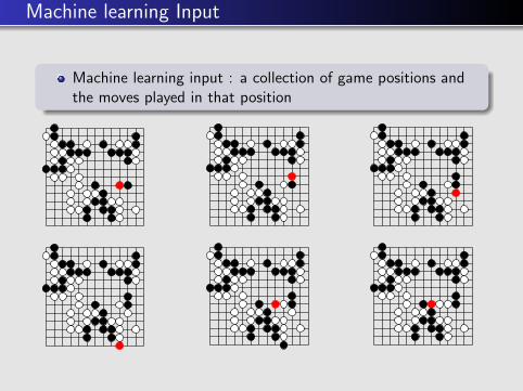
Machine learning Input
Machine learning input : a collection of game positions andthe moves played in that position
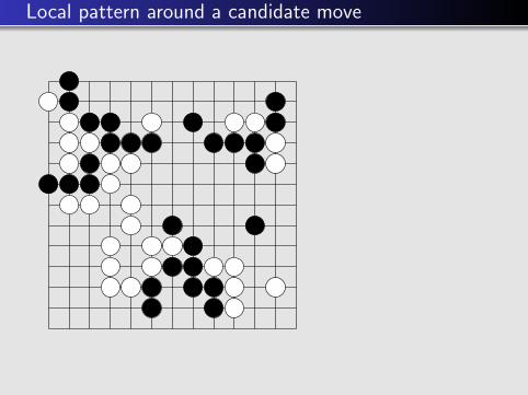
Local pattern around a candidate move
Red cell =candidate move
3x3 pattern aroundthe candidate move
Bigger pattern aroundthe candidate move

Local pattern around a candidate move
Red cell =candidate move
3x3 pattern aroundthe candidate move
Bigger pattern aroundthe candidate move

Local pattern around a candidate move
Red cell =candidate move
3x3 pattern aroundthe candidate move
Bigger pattern aroundthe candidate move

Local pattern around a candidate move
Red cell =candidate move
3x3 pattern aroundthe candidate move
Bigger pattern aroundthe candidate move

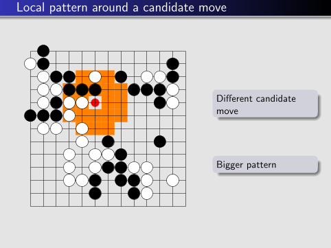
Local pattern around a candidate move
Different candidatemove
3x3 pattern
Bigger pattern

Local pattern around a candidate move
Different candidatemove
3x3 pattern
Bigger pattern
Local pattern around a candidate move
Different candidatemove
3x3 pattern
Bigger pattern

Machine learning
Machine learning idea
Compare the local patterns and learn evaluation weights
Local patterns of played moves better than local patterns ofnot-played moves

Machine learning
Machine learning idea
Compare the local patterns and learn evaluation weights
Local patterns of played moves better than local patterns ofnot-played moves

Machine learning features
Features
Local patterns are not sufficient
Generalization of patterns is called “features”
Examples of features
pattern shape
distance to the previous move
escape from immediate capture
... (secret ?)
Remi Coulom, Computing elo ratings of move patterns in the gameof go, 2007, ICGA Journal

Usage of Learned Knowledge
How can we include the learned knowledge?
Replace “Random simulations” by “realistic” simulations
Progressive Widening: limit the number of searched moves
Progressive Bias: search more some moves

Usage of Learned Knowledge
How can we include the learned knowledge?
Replace “Random simulations” by “realistic” simulations
Progressive Widening: limit the number of searched moves
Progressive Bias: search more some moves

Usage of Learned Knowledge
How can we include the learned knowledge?
Replace “Random simulations” by “realistic” simulations
Progressive Widening: limit the number of searched moves
Progressive Bias: search more some moves

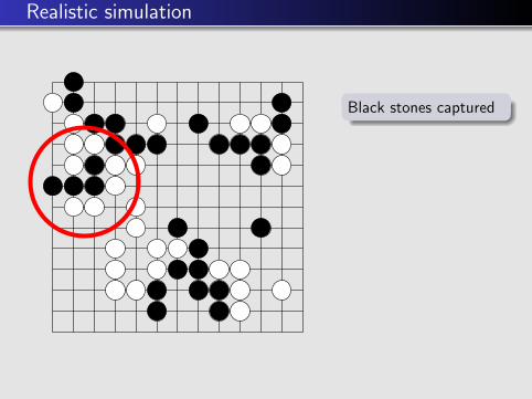
Realistic simulation
Black stones captured
⇒ should be capturedin all simulations
Random simulations:captured only in 50%of the simulations
Realistic simulations:almost always captured
Realistic simulation
Black stones captured
⇒ should be capturedin all simulations
Random simulations:captured only in 50%of the simulations
Realistic simulations:almost always captured

Realistic simulation
Black stones captured
⇒ should be capturedin all simulations
Random simulations:captured only in 50%of the simulations
Realistic simulations:almost always captured

Realistic simulation
Black stones captured
⇒ should be capturedin all simulations
Random simulations:captured only in 50%of the simulations
Realistic simulations:almost always captured

Realistic simulation
Black stones captured
⇒ should be capturedin all simulations
Random simulations:captured only in 50%of the simulations
Realistic simulations:almost always captured

Progressive Widening
Search only good candidates considering the learnedknowledge
Typically in 13× 13, only 15 moves searched

Progressive Widening
Search only good candidates considering the learnedknowledge
Typically in 13× 13, only 15 moves searched

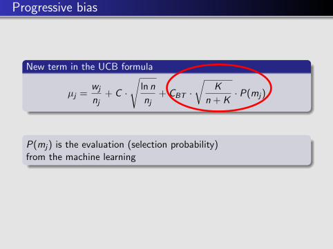
Progressive bias
New term in the UCB formula
µj =wj
nj+ C ·
√ln n
nj+ CBT ·
√K
n + K· P(mj)
P(mj) is the evaluation (selection probability)from the machine learning
⇒ Moves frequently played by professionals will be searched more

Progressive bias
New term in the UCB formula
µj =wj
nj+ C ·
√ln n
nj+ CBT ·
√K
n + K· P(mj)
P(mj) is the evaluation (selection probability)from the machine learning
⇒ Moves frequently played by professionals will be searched more
Progressive bias
New term in the UCB formula
µj =wj
nj+ C ·
√ln n
nj+ CBT ·
√K
n + K· P(mj)
P(mj) is the evaluation (selection probability)from the machine learning
⇒ Moves frequently played by professionals will be searched more

Progressive bias
New term in the UCB formula
µj =wj
nj+ C ·
√ln n
nj+ CBT ·
√K
n + K· P(mj)
P(mj) is the evaluation (selection probability)from the machine learning
⇒ Moves frequently played by professionals will be searched more

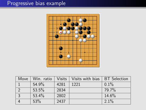
Progressive bias example
Move Win. ratio Visits Visits with bias BT Selection
1 54.9% 4281
1221 0.1%
2 53.5% 2834
15683 79.7%
3 53.4% 2802
1449 14.6%
4 53% 2437
365 2.1%

Progressive bias example
Move Win. ratio Visits Visits with bias BT Selection
1 54.9% 4281
1221 0.1%
2 53.5% 2834
15683 79.7%
3 53.4% 2802
1449 14.6%
4 53% 2437
365 2.1%

Progressive bias example
Move Win. ratio Visits Visits with bias BT Selection
1 54.9% 4281
1221
0.1%
2 53.5% 2834
15683
79.7%
3 53.4% 2802
1449
14.6%
4 53% 2437
365
2.1%
Progressive bias example
Move Win. ratio Visits Visits with bias BT Selection
1 54.9% 4281 1221 0.1%
2 53.5% 2834
15683
79.7%
3 53.4% 2802
1449
14.6%
4 53% 2437
365
2.1%

Progressive bias example
Move Win. ratio Visits Visits with bias BT Selection
1 54.9% 4281 1221 0.1%
2 53.5% 2834
15683
79.7%
3 53.4% 2802 1449 14.6%
4 53% 2437 365 2.1%
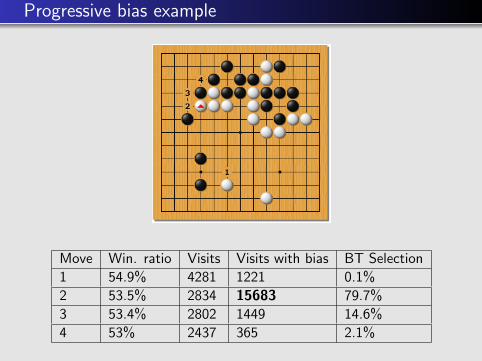
Progressive bias example
Move Win. ratio Visits Visits with bias BT Selection
1 54.9% 4281 1221 0.1%
2 53.5% 2834 15683 79.7%
3 53.4% 2802 1449 14.6%
4 53% 2437 365 2.1%

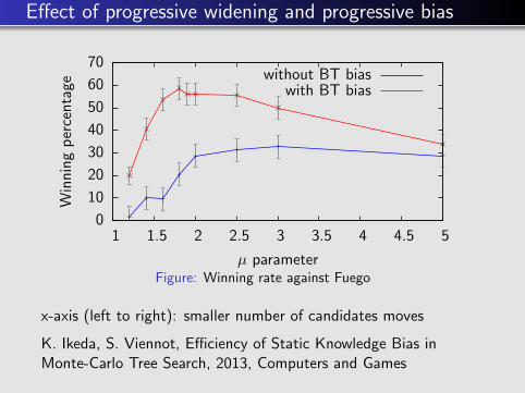
Effect of progressive widening and progressive bias
0
10
20
30
40
50
60
70
1 1.5 2 2.5 3 3.5 4 4.5 5
Win
nin
gp
erce
nta
ge
µ parameter
without BT bias
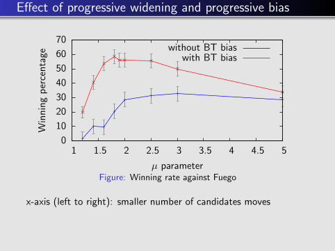
Figure: Winning rate against Fuego
x-axis (left to right): smaller number of candidates moves
K. Ikeda, S. Viennot, Efficiency of Static Knowledge Bias inMonte-Carlo Tree Search, 2013, Computers and Games
Effect of progressive widening and progressive bias
0
10
20
30
40
50
60
70
1 1.5 2 2.5 3 3.5 4 4.5 5
Win
nin
gp
erce
nta
ge
µ parameter
without BT biaswith BT bias
Figure: Winning rate against Fuego
x-axis (left to right): smaller number of candidates moves
K. Ikeda, S. Viennot, Efficiency of Static Knowledge Bias inMonte-Carlo Tree Search, 2013, Computers and Games

Section 5
Online Knowledge

Information extraction from the simulations
In MCTS, we collect the “winning ratio” information from therandom simulations
Simulations contain more information
Extracting this information can improve the search
Example of other information
Ownership
Criticality

Information extraction from the simulations
In MCTS, we collect the “winning ratio” information from therandom simulations
Simulations contain more information
Extracting this information can improve the search
Example of other information
Ownership
Criticality

Information extraction from the simulations
In MCTS, we collect the “winning ratio” information from therandom simulations
Simulations contain more information
Extracting this information can improve the search
Example of other information
Ownership
Criticality

Information extraction from the simulations
In MCTS, we collect the “winning ratio” information from therandom simulations
Simulations contain more information
Extracting this information can improve the search
Example of other information
Ownership
Criticality
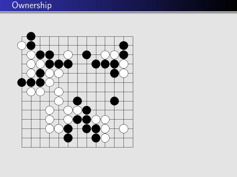
Ownership
Ownership =probability of“controlling an area”
Ownership boundary ≈territory boundary
(possible) usage
Search more the movesin the boundary

Ownership
Ownership =probability of“controlling an area”
Ownership boundary ≈territory boundary
(possible) usage
Search more the movesin the boundary

Ownership
Ownership =probability of“controlling an area”
Ownership boundary ≈territory boundary
(possible) usage
Search more the movesin the boundary

Ownership
Ownership =probability of“controlling an area”
Ownership boundary ≈territory boundary
(possible) usage
Search more the movesin the boundary

Criticality
Criticality =correlation between“controlling an area”and “winning”
Usage 1
Add moves from thecritical area to thesearch candidates
Usage 2
Search more thecritical moves

Criticality
Criticality =correlation between“controlling an area”and “winning”
Usage 1
Add moves from thecritical area to thesearch candidates
Usage 2
Search more thecritical moves

Criticality
Criticality =correlation between“controlling an area”and “winning”
Usage 1
Add moves from thecritical area to thesearch candidates
Usage 2
Search more thecritical moves

Criticality
Criticality =correlation between“controlling an area”and “winning”
Usage 1
Add moves from thecritical area to thesearch candidates
Usage 2
Search more thecritical moves
Section 6
Examples of current problems

Problem 1

Problem 2
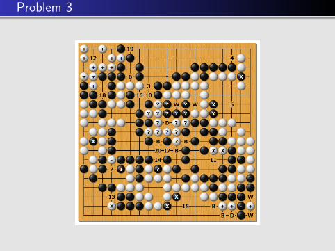
Problem 3
Section 7
Conclusion

Conclusion
Knowledge extraction
from professional game records with machine learning
from the simulations
included both in the simulations and in the search algorithm
⇒ strong programs
How far are we from professionals ?

Conclusion
Knowledge extraction
from professional game records with machine learning
from the simulations
included both in the simulations and in the search algorithm
⇒ strong programs
How far are we from professionals ?
Conclusion
Knowledge extraction
from professional game records with machine learning
from the simulations
included both in the simulations and in the search algorithm
⇒ strong programs
How far are we from professionals ?

Conclusion
Knowledge extraction
from professional game records with machine learning
from the simulations
included both in the simulations and in the search algorithm
⇒ strong programs
How far are we from professionals ?

Conclusion
Knowledge extraction
from professional game records with machine learning
from the simulations
included both in the simulations and in the search algorithm
⇒ strong programs
How far are we from professionals ?

Conclusion
Knowledge extraction
from professional game records with machine learning
from the simulations
included both in the simulations and in the search algorithm
⇒ strong programs
How far are we from professionals ?

Denseisen
Computer-Human match
Top 2 programs of UEC-cup
Against top professionals
With handicap
4-stone handicap games
2013 and 2014 : Crazystone wins, Zen loses
article in Wired “The Mystery of Go”

Denseisen
Computer-Human match
Top 2 programs of UEC-cup
Against top professionals
With handicap
4-stone handicap games
2013 and 2014 : Crazystone wins, Zen loses
article in Wired “The Mystery of Go”

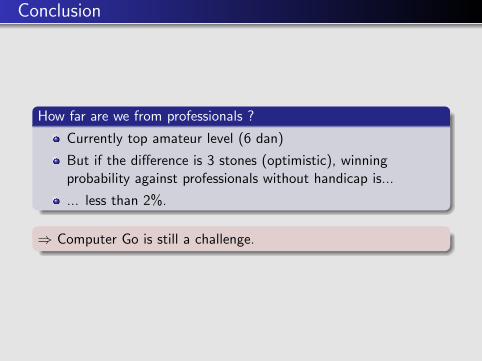
Conclusion
How far are we from professionals ?
Currently top amateur level (6 dan)
But if the difference is 3 stones (optimistic), winningprobability against professionals without handicap is...
... less than 2%.
⇒ Computer Go is still a challenge.

Conclusion
How far are we from professionals ?
Currently top amateur level (6 dan)
But if the difference is 3 stones (optimistic), winningprobability against professionals without handicap is...
... less than 2%.
⇒ Computer Go is still a challenge.

Conclusion
How far are we from professionals ?
Currently top amateur level (6 dan)
But if the difference is 3 stones (optimistic), winningprobability against professionals without handicap is...
... less than 2%.
⇒ Computer Go is still a challenge.

Conclusion
How far are we from professionals ?
Currently top amateur level (6 dan)
But if the difference is 3 stones (optimistic), winningprobability against professionals without handicap is...
... less than 2%.
⇒ Computer Go is still a challenge.
Conclusion
How far are we from professionals ?
Currently top amateur level (6 dan)
But if the difference is 3 stones (optimistic), winningprobability against professionals without handicap is...
... less than 2%.
⇒ Computer Go is still a challenge.

Conclusion
Thank you for listening.Any questions ?

References
1993, Brugmann, Monte-Carlo Go
2003, Bouzy, Helmstetter, Monte-Carlo Go developments
2006, Kocsis, Szepesvari, Bandit based Monte-Carlo planning
2006, Gelly, Teytaud et al, Modification of UCT with patternsin Monte-Carlo Go
2007, Coulom, Computing ELO ratings of move patterns inthe game of Go
2007, Gelly, Silver, Combining online and offline knowledge inUCT
2009, Coulom, Criticality - a Monte-Carlo heuristic for Goprograms
2011, Petr Baudis, Master thesis, MCTS with informationsharing
2012, Browne et al, A Survey of Monte Carlo Tree SearchMethods