the role of lithological layering and pore pressure on

The role of lithological layering and pore pressureon fluid-induced microseismicityV. Roche1 and M. van der Baan1

1Department of Physics, CCIS, University of Alberta, Edmonton, Alberta, Canada

Abstract The success of hydraulic fracturing treatments is often judged by the shape and size of theresulting microseismic cloud. However, it is challenging to predict the anticipated microseismic cloud priorto treatment. We use geomechanical modeling to predict the distribution of the microseismicity prior to thehydraulic fracture treatment. We analyze the likelihood of tensile and shear failure due to 1-D variations inlocal stresses and rock strengths, induced by layering and pore pressure, for two field cases. The deviation inthe local stresses from the regional stress field is induced by vertical variations in stiffness. This promotesfailure of the stronger layers instead of the weaker ones since the stronger layers can become essentially loadbearing. The simulations and field studies show that (1) microseismic events tend to locate preferentiallywhere layers reach tensile failure due to fluid injection, and the number of events tends to decrease in layersthat do not reach tensile failure; (2) shear initiation can occur in different layers from those failing in tension,thereby creating additional fluid migration paths; and (3) reactivation of preexisting fractures may occur dueto fluid migration, even if their orientations are unfavorable. Numerical modeling is a significant aid inunderstanding the interplay of regional and local stresses and associated in situ failure due to variations inrock strength, pore pressure, and stiffnesses. In a wider perspective, it gives fundamental insights into theunderstanding of earthquakes and fault localization, the mechanisms of fracture development, and the roleof fractures on fluid circulation and on the in situ stress field.

1. Introduction

The successful development of the shale-gas and shale-oil plays in North America has radically changed itsenergy landscape. This has been achieved in part due to technological innovations in combining directionaldrilling and hydraulic fracturing. This process involves forced fluid injection into hydrocarbon reservoirs toincrease the rock permeability through the opening of fractures due to brittle failure and slip within the hostrock [Pearson, 1981; King, 2010]. It is also applied to extract geothermal energy [Majer et al., 2007; Yoon et al.,2014] or to facilitate underground block caving in mines [Kaiser et al., 2011; Preisig et al., 2014]. A cloud oflow-magnitude microseismic events (i.e., M< 0) develops during the fluid injection, and its analysis givesinsights into the location, shape, time dependence, and failure mechanism of the developing fractures withinthe reservoir rock [Pearson, 1981; Phillips et al., 2002; Davies et al., 2012]. The temporal and spatial developmentof the microseismic cloud as well as the failure mechanisms of the individual events permit assessment ofthe performance of the hydraulic fracturing process, cap rock integrities, and provide pertinent information onfluid leak off and the presence of triggered earthquakes [Cipolla et al., 2009; King, 2010;Davies et al., 2012; Shuklaet al., 2010; Van der Baan et al., 2013].

The size and shape of the microseismic cloud has, however, proven difficult to predict prior to the hydraulicfracturing treatment [Fisher and Warpinski, 2011; Davies et al., 2012; Eaton et al., 2014b]. In this paper we analyzeits vertical variability. It often exhibits correlation to the layering: in some cases the microseismicity is constrainedto specific horizontal layers despite that hydraulic fracturing treatment also occurs in intermediate layers andthe amount of microseismicity may decrease or increase vertically reflecting lithological layering [Phillips et al.,1998; Rutledge and Phillips, 2003; Fischer et al., 2008; Pettitt et al., 2009]. In other scenarios out-of-zonegrowth occurs, where the microseismic cloud spreads out beyond the reservoir layer and the immediatetreatment zone [Fisher and Warpinski, 2011; Eaton et al., 2014b]. Out-of-zone growth is generally unwantedsince it implies fluid containment challenges [Fisher and Warpinski, 2011; Davies et al., 2012].

Several methodology based on well log data may be used in order to investigate the influence of layeredsedimentary structures. This includes analysis of a brittleness index [Rickman et al., 2008; Mullen et al., 2007;

ROCHE AND VAN DER BAAN ©2015. American Geophysical Union. All Rights Reserved. 923

PUBLICATIONSJournal of Geophysical Research: Solid Earth

RESEARCH ARTICLE10.1002/2014JB011606

Key Points:• The role of lithological layering onfluid-induced fractures andmicroseismicity

• Two field cases• Effects of natural layered sequenceson in situ local stresses and failures

Correspondence to:V. Roche,[email protected]

Citation:Roche, V., and M. van der Baan (2015),The role of lithological layering and porepressure on fluid-inducedmicroseismicity,J. Geophys. Res. Solid Earth, 120, 923–943,doi:10.1002/2014JB011606.

Received 12 SEP 2014Accepted 29 DEC 2014Accepted article online 7 JAN 2015Published online 3 FEB 2015

http://publications.agu.org/journals/

http://onlinelibrary.wiley.com/journal/10.1002/(ISSN)2169-9356

http://dx.doi.org/10.1002/2014JB011606

http://dx.doi.org/10.1002/2014JB011606

Cho and Perez, 2014] and in situ stress calculation [Blanton and Olson, 1999; Beaudoin et al., 2011; Song andHareland, 2012]. In this paper we analyze the role of vertical strength variations, the in situ local stress state,and the pore pressure. These parameters are critical in fracture development [Teufel and Clark, 1984; Bourne,2003; Roche et al., 2013] and earthquake localization, triggering, and their magnitudes [Sibson, 1982;Zakharova and Goldberg, 2014; Langenbruch and Shapiro, 2014]. For simplicity we ignore many of theindividual treatment parameters, such as the type of fracturing fluid and its viscosity, the presence ofproppant, the exact injection strategy including the number of stages along a borehole and the injectionpressure fluctuations in the individual stages, whether wells are stimulated sequentially or simultaneouslyusing a zip pattern in case of treatment of multiple horizontal wells. All these variations have beenobserved to affect the resulting microseismic cloud [Warpinski et al., 2004; Cipolla et al., 2009; Calò et al.,2011]. In addition, we will also ignore fluid leak-off effects into the rock matrix and the type ofhydrocarbons in the reservoir (gas and oil) such that we can treat the medium as elastic.

As a base hypothesis we postulate that the shape of the microseismic cloud is foremost determined by themechanical properties of the medium and the in situ effective stresses, whereas fluid diffusion effects andtreatment parameters are paramount for explaining and forecasting the behavior of the individual eventsand thus the fine detail of the spatial and temporal evolution of the microseismic cloud. This hypothesisallows us to appeal to similar numerical modeling methods also invoked to study fault nucleation,propagation, and termination [Teufel and Clark, 1984; Bourne, 2003; Roche et al., 2013], without the need toincorporate many of the more challenging effects into our modeling strategy due to inherent complexities inthe hydraulic fracturing treatments. Conversely, it extends beyond previous fault modeling from Roche et al.[2013] by explicitly incorporating the effect of the in situ pore pressure on fracture and failure development.

Such an elastic approach allows us to compute the most likely microseismic locations based on informationavailable prior to hydraulic fracturing. It provides a first prediction of anticipated microseismicity, therebyallowing for a better interpretation of the actual recorded microseismicity. In a wider perspective, it yieldsenhanced insights into the role of fluids on earthquakes and faulting, and complements other studiesfocusing on explaining the spatial distribution of recorded seismicity given the local geology and stress state[Segall and Pollard, 1980; Sibson, 1982; Zakharova and Goldberg, 2014; Langenbruch and Shapiro, 2014].

In this paper, we use a numerical modeling approach similar to Roche et al. [2013]. We model the effect oflithological layering on the in situ stress and its effect on the likelihood of tensile and shear failure in eachlayer. The analysis takes into account the overburden, the pore pressure, and tectonic solicitation. In themodel the tectonic effects are assumed stress driven instead of strain driven [Blanton and Olson, 1999;Beaudoin et al., 2011; Song and Hareland, 2012]. We compare the results with the vertical distribution of themicroseismic event clouds produced during two hydraulic fracturing treatments in two different stressregimes, namely, strike slip and normal faulting. The first case history has microseismic events constrained tospecific horizontal layers, whereas the second case deals with out-of-zone growth. In addition, the two casestudies illustrate the role of depletion and in situ pore pressures on the resulting microseismic distributions.

First we describe the geologic settings of both case histories and the recorded microseismicity. Next, wedetail the modeling strategy, and then we analyze the numerical results in terms of the effects of lithologicallayering and vertical strength variations on differential stress concentrations, likelihood of shear and tensilefailure, and the resulting anticipated microseismic clouds.

2. Two Studied Natural Cases2.1. Geological Settings of the Two Studied Sites

Two naturally layered field examples are investigated. The first one is called Case 1 for confidentiality. It islocated in the Western Canadian sedimentary basin that is a northeast-southwest trending clastic wedge(central Alberta, Canada) [Mossop and Shetsen, 1994]. In the studied stratigraphic sequence, the reservoir rockis tight sandstone from the Glauconitic formation of the Lower Cretaceous Mannville group (Figure 1) [Hayeset al., 1994]. It is part of the Hoadley barrier complex and overlying the Ostracod formation limestone. TheMedicine River coal, the Manville shale, the Joli Fou shale, and the Viking sandstone formations compose theoverlying stratigraphic column investigated here (Figure 1). The basin is within a strike-slip stress regime witha maximum horizontal stress oriented N060 in the studied area [Bell and Bachu, 2003; Ristau et al., 2007]. The

Journal of Geophysical Research: Solid Earth 10.1002/2014JB011606


reservoir is partially underpressurized. As a result, the hydraulic pressure gradient k ranges from 10 kPam�1

to 5 kPam�1 with a mean of 6 kPam�1 [Woodland and Bell, 1998].

The second field is the Carthage Cotton Valley field, called Case 2. The formation is within the northern Gulf ofMexico basin (east Texas, USA) (Figure 1). It comprises several low-permeability reservoir sands within aninterbedded sequence of sands and shales of the Jurassic Cotton Valley formation (Figure 1). The CarthageCotton Valley field is a structural province of gently dipping beds, open periclinal folds, and normal faultsattributed to diapiric movement of salt [Rutledge and Phillips, 2003]. The area is believed to be within anormal-faulting stress regime with minimum horizontal stress oriented north-northwest with azimuthapproximately N010 [Zoback and Zoback, 1980; Gough and Bell, 1982; Rutledge and Phillips, 2003]. Thehydraulic gradient k ranges from 9.7 kPam�1 to 12 kPam�1 [Dyman and Condon, 2006], which is close to thehydrostatic pore pressure condition (i.e., k equals 10 kPam�1).

2.2. Vertical Distribution of the Microseismic Events

In Case 1, a multistage hydraulic fracture treatment program is performed in two horizontal wells.Microseismic data are acquired by real-time microseismic monitoring using a 12 sensor downhole array of

Figure 1. Distribution of the microseismic events and layering of the two field examples. (a–c) Data for Case 1; (d–f ) related to the Carthage Cotton Valley Field.Figures 1a and 1d show the distribution of the microseismic events along major axis of the microseismic cloud (direction of longest elongation). Figures 1b and1e show depth distribution of the microseismic events. The perforation zones are indicated (white bars). Figures 1c and 1f show stratigraphic section for the twostudied areas indicating the lithological sequence used in the modeling. Figures 1d and 1e from Rutledge and Phillips [2003].



triaxial geophones. The geophone pods are deployed from 1605m to 1835m depth in a vertical monitor welllocated between the two treatment wells and usemagnets to achieve coupling with the steel wellbore casing[Eaton et al., 2014a]. One thousand six hundred sixty events are used with location accuracies around 20mwith a standard deviation of 15m (Figures 1a and 1b).

Case 2 has also multiple fracturing stages, but within a single vertical borehole. We use the verticaldistribution of microseismic events from the stage 3 completion described by Rutledge and Phillips [2003].Details on the instrumentation design and installation are presented in Walker [1997]. Six hundred eventshave been recorded during the stage. Figures 1d and 1e show the along-strike cross section and the depthdistribution of the microseismic events.

In both cases, the number of events is always high around the injection depths. It reaches 9% (153 events)within a 6m interval in Case 1. In case 2, 53% of events occur within a total of 22m of injection, ranging from1% to 21% for the individual injection depths. Away from the injections in Cases 1 and 2, respectively,91% and 47% of the events occur in different layers. Significant out-of-zone growth occurs in Case 1. Thefarthest events are recorded around 100m above and 60m below the injection point for Case 1 and around15m vertically from the injection points for Case 2.

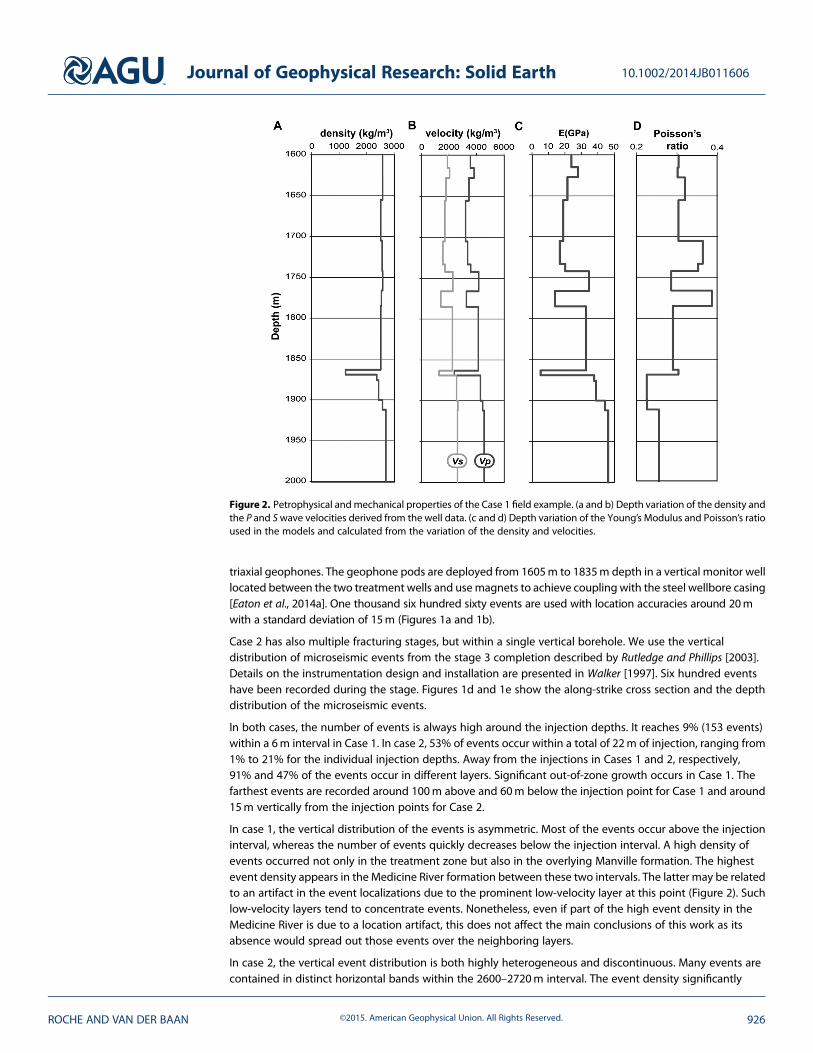
In case 1, the vertical distribution of the events is asymmetric. Most of the events occur above the injectioninterval, whereas the number of events quickly decreases below the injection interval. A high density ofevents occurred not only in the treatment zone but also in the overlying Manville formation. The highestevent density appears in the Medicine River formation between these two intervals. The latter may be relatedto an artifact in the event localizations due to the prominent low-velocity layer at this point (Figure 2). Suchlow-velocity layers tend to concentrate events. Nonetheless, even if part of the high event density in theMedicine River is due to a location artifact, this does not affect the main conclusions of this work as itsabsence would spread out those events over the neighboring layers.

In case 2, the vertical event distribution is both highly heterogeneous and discontinuous. Many events arecontained in distinct horizontal bands within the 2600–2720m interval. The event density significantly

Figure 2. Petrophysical andmechanical properties of the Case 1 field example. (a and b) Depth variation of the density andthe P and Swave velocities derived from the well data. (c and d) Depth variation of the Young’s Modulus and Poisson’s ratioused in the models and calculated from the variation of the density and velocities.



decreases in some intermediate intervals and events are even completely absent in some layers, despiteproximity to the injection perforations.

In both cases, there is no clear link between event distribution and the strength of a layer. Events concentrateboth in some weak shales and coal layers as well as some strong sandstones and limestones. Likewise thevertical distributions of microseismic events deviate significantly from what we would expect in homogeneousisotropic nonfractured rocks where the number of events decreases monotonically with vertical distance fromthe injection points. We investigate if observed vertical variations in microseismic distributions are caused bythe initial regional stress state, in situ stress concentrations due to local changes in rock stiffnesses, lithologicalstrength variations, and/or the hydraulic pressure gradient.

3. Modeling Design and Input3.1. Modeling Strategy

We use a discrete-element method to calculate the stresses and strains inside discontinuous media [Cundall,1992]. We simulate the in situ local stress field due to one-dimensional variations in elastic properties imposedby the lithological layers [Teufel and Clark, 1984; Bourne, 2003; Roche et al., 2013]. The elastic behaviors aredetermined by the Young’s moduli and Poisson’s ratios calculated using well logs. The one-dimensional elasticmodel is then submitted to boundary conditions that reflect the appropriate regional horizontal and vertical

Figure 3. (a–d) Petrophysical and mechanical properties of the Carthage Cotton Valley Field. Same legend as Figure 2. Theblocked continuous lines in Figures 3c and 3d show the 1-D variations in the Young’s modulus and Poisson’s ratio used inthe discrete-element model.



stresses and estimates for the in situpore pressure prior to fluid injection asderived from the hydraulic gradient.The numerical models provide theexpected in situ local stresses as afunction of depth. We examine theeffect of dry rocks (i.e., zero porepressure), underpressured rocks, andhydrostatic pore pressures todemonstrate the effect of pore pressureprior to injection on the expectedeffective stress distributions.

Next we invoke the Mohr-Coulomband Griffith’s failure criteria to computethe likelihood of, respectively, shearand tensile failure as a function ofdepth using appropriate estimatesof the tensile strength and cohesionof the local lithologies. We add theinjection pressure to the entire sectionto obtain an upper bound on theshape of the expected microseismic

cloud. We then compare these failure predictions with the recorded microseismicity. The various steps of thismodeling strategy are detailed in the next subsections.

3.2. Elastic Layered Sections

The depth dependence of the dynamic elastic parameters, Young’s modulus E, and Poisson’s ratio ν arecalculated from the density ρ, the compressional and shear wave velocities, Vp and Vs, respectively, asobtained from blocked well data (Figures 2 and 3), with the following equations:

G ¼ ρVS2; λ ¼ ρVP

2 � 2G; E ¼ G 3λþ 2Gð ÞGþ λð Þ ; ν ¼ λ

2 Gþ λð Þ ; (1)

where G and λ are the shear modulus and Lame’s first parameter, respectively. The wave velocities Vp and Vscorrespond to the vertical velocities and we assume that Vp, Vs, E, and v are isotropic. Justification for variousassumptions implied in the use of equation (1) such as using dynamic instead of static elastic propertiesare postponed to the discussion section.

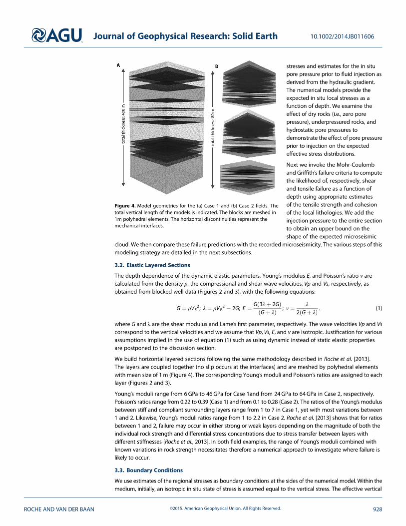
We build horizontal layered sections following the same methodology described in Roche et al. [2013].The layers are coupled together (no slip occurs at the interfaces) and are meshed by polyhedral elementswith mean size of 1m (Figure 4). The corresponding Young’s moduli and Poisson’s ratios are assigned to eachlayer (Figures 2 and 3).

Young’s moduli range from 6GPa to 46GPa for Case 1and from 24GPa to 64GPa in Case 2, respectively.Poisson’s ratios range from 0.22 to 0.39 (Case 1) and from 0.1 to 0.28 (Case 2). The ratios of the Young’s modulusbetween stiff and compliant surrounding layers range from 1 to 7 in Case 1, yet with most variations between1 and 2. Likewise, Young’s moduli ratios range from 1 to 2.2 in Case 2. Roche et al. [2013] shows that for ratiosbetween 1 and 2, failure may occur in either strong or weak layers depending on the magnitude of both theindividual rock strength and differential stress concentrations due to stress transfer between layers withdifferent stiffnesses [Roche et al., 2013]. In both field examples, the range of Young’s moduli combined withknown variations in rock strength necessitates therefore a numerical approach to investigate where failure islikely to occur.

3.3. Boundary Conditions

We use estimates of the regional stresses as boundary conditions at the sides of the numerical model. Within themedium, initially, an isotropic in situ state of stress is assumed equal to the vertical stress. The effective vertical

Figure 4. Model geometries for the (a) Case 1 and (b) Case 2 fields. Thetotal vertical length of the models is indicated. The blocks are meshed in1m polyhedral elements. The horizontal discontinuities represent themechanical interfaces.



stress σv′ is obtained by integratingthe density logs and subtracting thein situ pore pressure before hydraulicfracturing. For simplicity we assumean average density in both Case 1 andCase 2; that is,

σv ’ zð Þ ¼ ρgz � P0 zð Þ: (2)

The in situ pore pressure P0 dependson the predefined pressure gradient kand the depth z:

P0 zð Þ ¼ zk; (3)

The next step involves setting the ratiosof the effective remote regional stressesσ1r,0, σ2r,0, σ3r,0. They are computedrelative to the effective vertical stress σv′assuming a critical, frictional andcohesionless state of stress of the brittlecrust [Sibson, 1974; Brudy et al., 1997;Zoback, 2007] with the followingsystem of equations:

σ1r;0 � σ3r;0� �

2

� � ffiffiffiffiffiffiffiffiffiffiffiffiffiffiffiffiffi1þ μ²ð Þ

q

�μσ1r;0 þ σ3r;0� �

2

� �¼ 0;

σ1r;0 þ σ3r;0� �

2¼ σ2r;0

(4)

where σ1r,0 and σ2r,0 equals σv′ forextension and strike-slip regimes,respectively. The internal coefficient offriction μ is set to 0.7. For notationalconvenience we have dropped thesuperscript ’ to indicate that we areusing the effective stresses. Figure 5ashows a theoretical Mohr-Coulombcircle corresponding to the imposedregional boundary conditions for a

normal stress regime. In our notation for stress, the first index (1, 2, 3) indicates, respectively, the maximum,intermediate, or minimum principal stress; the second index (r or l) specifies whether this is a regional or localstress; and the third index (0 or i) if this is a preinjection or postinjection stress. The depth-dependent localstresses are defined as those computed by the discrete-element model at the central surface location afterapplication of the boundary stresses.

We analyze various pore pressure scenarios for both Case 1 and Case 2 since the actual pore pressures at the timeof the hydraulic fracturing treatment are not always well known. A total of five models are considered withdifferent preinjection pore pressure gradients k (Table 1). For both cases, we use a first set of models with gradientk set to null. This condition simulates the case of no fluidswithin the rocks before injection. A second set ofmodelsassumes a hydrostatic pore pressure (i.e., k=10kPam�1). This model is likely to reproduce the in situ condition forCase 2. Both sets of models are considered end members to address variations in the effective stresses due toexisting pore pressures prior to injection. The effective stresses are equal to the absolute ones for k=0kPam�1

but significantly reduced when k=10kPam�1. Finally, for Case 1, we consider a model with gradient k equal to6 kPam�1 that likely reproduces the actual in situ conditions for a underpressurized reservoir. We do not consider

Figure 5. Mohr-Coulomb circles illustrating the stress evolution for anormal stress regime. (a) Critical initial remote state of stress used asboundary condition. (b) Modification in the local stresses at the center ofthe model due to lithological layering. (c) Stress modifications due to fluidinjection. In Figures 5b and 5c the dark and light grey circles representthe state of stress in compliant and stiff layers, respectively. The σv′ is thevertical stress. The σ1r,0, σ2r,0, and σ3r,0 are the boundary remote stressesapplied on the face of the models. The σ1l,0, σ2l,0, and σ3l,0 are the localstate of stress perturbed by the layering and before fluid injection. The σ1l,i,σ2l,i, and σ3l,i are the local effective stresses after the fluid injection. P0 andΔP are the in situ pore pressure and fluid pressure perturbation due toinjection. The white and grey arrows represent stress modifications due tofluid effects and layering, respectively.



overpressured reservoirs as these are lesslikely for the two field examples. Theboundary stresses applied on themodelsare shown in Figure 6.

3.4. Fluid Injection

The discrete-element methodcomputes the effective local stressesσ1l,0, σ2l,0, and σ3l,0 affected by stresstransfer, given the imposed regionalstress field, pore pressure gradients,and mechanical properties for eachcase study (Figure 5b). In order toassess the likelihood of tensile and

shear failure, we also take themechanical effect of the injection pressure into account. We use a single valueof the bottomhole fluid pressure Pi averaged over all stages. It equals 28MPa and 40MPa for Cases 1 and 2,respectively. In Case 1, the bottomhole pressure ranges from 62MPA to 21MPA with a standard deviation of3MPA (29,000 data points). In Case 2, it ranges from 42MPA to 33MPA with a large part comprised between38 and 42MPA [Rutledge and Phillips, 2003].

The bottomhole pressure represents the sum of all the pressures exerted at the bottom of the hole, includingthe preinjection in situ pore pressure but also viscous drag and friction involved in creating fluid leak off intothe rock. The effective maximum increase in the pore pressure due to the fluid injection (ΔP) is thus

ΔP ¼ Pi � P0 zð Þ; (5)

where P0(z) is computed using equation (2). In Case 2, fluid injections occur at various depths, and we use theaveraged depth of the sequence to compute a single pore pressure perturbation ΔP. The effective increase inpore pressure depends on the preinjection pore pressure. It is therefore equal to the bottomhole pressure for thedry model (k=0kPam�1) but significantly reduced when the rock is filled with fluids (k=6 or 10 kPam�1).

Table 1. General Characteristic of the Five Models Considered

Study CaseStressRegime

DepthInterval (m)

In Situ PorePressurea

Case 1 strike slip 1600–2000 dry: k = 0 kPam�1

depletion:k = 6 kPam�1

hydrostatic:k = 10 kPam�1

Case 2 normal fault slip 2600–2720 dry: k = 0 kPam�1

hydrostatic:k = 10 kPam�1

aData in bold likely reflect best the in situ conditions.

Figure 6. Boundary conditions applied on the model sides. (a and d) The boundary conditions (regional stresses) for the models without in situ fluids (i.e., k = 0), forCase 1 and 2, respectively. (b) The conditions for Case 1 anticipating partial depletion (i.e., k = 6 kPam�1). (c and e) The effective regional stresses assuminghydrostatic pore pressures (i.e., k = 10 kPam�1), for the Case 1 and 2, respectively. The light grey triangles, the medium grey dots, and the dark grey squares are themaximum, intermediate, and minimum effective boundary stresses, σ1r,0, σ2r,0, and σ3r,0, respectively.



The pressure perturbation ΔP due to fluid injection is then subtracted from the computed local stresses toobtain an upper bound on the area where failure is expected. The new local effective stresses after the injectionσ1l,i, σ2l,i, and σ3l,i are thus obtained from the preinjection effective local principal stresses (σ1l,0, σ2l,0, and σ3l,0)and the increase in pore pressure ΔP due to injection (Figure 5c) using

σ1 l:i ¼ σ1 l;0 � ΔP; σ2 l;i ¼ σ2 l;0 � ΔP; andσ3 l;i ¼ σ3 l ;0 � ΔP: (6)

We assume that ΔP is constant everywhere to calculate the local effective stresses. This assumes porepressure diffusion of the injected fluids throughout the medium.

3.5. Failure Criteria

We use the Coulomb failure criterion Cc and the simplified Griffith criterion Gc to estimate the likelihood oflocal shear and tensile failure, respectively, given all considered pore pressure scenarios (dry,underpressurized, and hydrostatic pressures). Failure occurs if Cc and Gc satisfy either of the two followingconditions [Jaeger et al., 2007]:

σ1 l;i � σ3 l;i� �

2

� � ffiffiffiffiffiffiffiffiffiffiffiffiffiffiffiffiffi1þ μ²ð Þ

q� μ

σ1 l;i þ σ3 l;i� �

2

� �� S ¼ Cc ¼ 0; σ3 l;i � T ¼ Gc ¼ 0; (7)

where σ1l,i and σ3l,i are the local effective stresses after fluid injection. We analyze the likelihood of failure as afunction of depth to determine where microseismic events are most likely to occur. We postulate that thelikelihood of failure increases with increasing positive values of criteria Cc and Gc.

Failure criteria Cc andGc depend on the internal coefficient of friction μ, cohesion S,, and tensile strengthTwhichcharacterize the rock strength properties. We use representative values from the literature (Table 2) andevaluate robustness of predictions by considering minimum, average, and maximum rock strengths. Thelithological sections are shown in Figures 1c and 1f. They are constrained from the literature and the well data.

4. Local Stress State Before Injection4.1. Effect of Lithological Layering

Figure 7 shows the computed local stresses before fluid injection as a function of depth and the preinjectionpore pressures for each site. The trends in the local stresses due to the lithological layering are similar for allpore pressure conditions. On the other hand, the effective local stresses obviously decrease with increasingpore pressures. In Case 1, the magnitude of the simulated minimum principal stress ranges from 9MPa to17MPa in the Glauconite formation, depending on the pore pressure. These values are lower than thepublished 20.5MPa magnitude for the minimum horizontal stress derived from well measurements [Bell andBachu, 2003]. In Case 2, the magnitude of the simulated minimum principal stresses ranges from 20MPa to39MPa and from 20MPa to 34MPa at 2640 and 2690m depth, respectively, which is close to the publishedvalues derived from well measurements being 33MPa and 35MPa, respectively [Mayerhofer et al., 2000].For both cases the published horizontal minimum stress values are close to the simulated local stresses fordry rocks but they are underestimated for the fluid scenarios.

The local vertical principal stresses σ2l,0 and σ1l,0, for the strike-slip (Case 1) and extension (Case 2) regimes,respectively, remain largely unchanged from the imposed regional vertical stresses (compare Figure 6 andFigure 7). Conversely, the horizontal stresses change due to the layering. This is caused by the stiffness contrastthat produces stress transfer from one layer to the other, thereby affecting the local horizontal stresses.

Table 2. The Strength Properties of the Rocks Used in the Layered Sections

Rock Internal Frictiona Cohesionb, S (MPa) Tensileb, T (MPa)

Sandstones 0.7 (0.45–1) 45 (30–70) 6 (4–10)Shales 0.45 (0.15–1.4) 35 (25–55) 2 (1–10)Coal 0.45 (0.15–1.4) 20 (15–25) 1 (1–3)Limestones 0.7 (0.35–1) 45 (25–70) 12 (4–18)

aThe values in brackets represent lower and upper bounds derived from representative rock samples from Einstein andDowding [1981].

bThe values in brackets represent lower and upper bounds derived from representative rock samples from Lockner [1995].



For the strike-slip regime, the horizontal stress σ3l,0 (Figure 7a) increases in the compliant layers due to anadditional layer-parallel compressive stress which restrains these layers from further elongation. In return,σ3l,0 decreases in the stiffer layers because of the introduction of an additional layer-parallel tensile stress dueto the elongation imposed by the softer layer. Conversely, horizontal stress σ1l,0 increases in the compliantlayers and decreases in the stiff layers. This is due to additional layer-parallel compressive and tensile stressescaused by the difference in shortening between the compliant and stiff layers.

For the extension regime, the horizontal stresses (i.e., σ3l,0 and σ2l,0) increase locally in the compliant layersbecause of the creation of an additional layer-parallel compressive stress which restrains these layers fromfurther elongation. In return, the stiffer layers acquire locally an additional layer-parallel tensile stress due tothe elongation imposed by the softer layers and horizontal stresses decrease in such layers (Figure 7b).Such variations are in agreement with observations obtained on a pile of coupled layers [Teufel and Clark,1984; Mandl, 1988; Evans et al., 1989; Cornet and Burlet, 1992; Bourne, 2003; Gunzburger and Cornet, 2007;Welch et al., 2009].

4.2. Magnitude of the Stress Concentrations

In all models, the variation in the local stresses does not result in stress permutation within any layer and thelocal stress regime stays similar to the regional one. The magnitude of the change in principal stresses due tothe layering depends on the contrast in the Young’s moduli between surrounding layers. For instance, thestress change is largest in a stiff layer surrounded by two highly compliant layers, or in a compliant layersurrounded by two highly stiff layers. As a consequence, the range in stress changes increases with thestiffness contrast between compliant and stiff layers within the layered media. In addition, the change instress also depends on the thickness of the layers [Roche et al., 2013].

Figure 7. Variation in the local stresses with depth, extracted from the center of the model. (a and b) The results for Cases 1 and 2, respectively. The σ1l,0, σ2l,0, andσ3l,0 are the maximum, intermediate, and minimum principal stresses before fluid injection. The various greys correspond to the different pore pressureconditions. Dark grey: no fluids in the rocks (k = 0); medium grey: underpressurized conditions (k = 6 kPam�1); light grey: hydrostatic pore pressure conditions(k = 10 kPam�1). The black stars indicate measurements of the minimum horizontal principal stress obtained from well data from Bell and Bachu [2003] andMayerhofer et al. [2000].



In the entire Case 1 sequence, σ1l,0 ranges from 50MPa to 80MPa for the dry case (Figure 7a). For the modelwith hydrostatic in situ pore pressure, σ1l,0 is lower and ranges from 30MPa to 49MPa. Similar ranges areobserved for σ3l,0 that ranges from 5MPa to 42MPa and from 3MPa to 25MPa for the dry and hydrostatic insitu pore pressures cases, respectively. The Case 2 sequence displays similar tendency (Figure 7b). The σ3l,0ranges from 1MPa to 38MPa and from 1MPa to 23MPa for the dry and hydrostatic in situ pore pressurescases, respectively. The σ2l,0 ranges from 31MPa to 54MPa and from 19MPa to 32MPa for the dry andhydrostatic in situ pore pressures cases, respectively. The depth variation in horizontal stresses is partlyassociated with both an increase in the overburden stresses and the variations in the stiffness contrasts. Inorder to analyze the local variation from layer to layer and to compare them to the literature, we calculate alocal change in percentage (see Table 3).

The maximum variation of the effective maximum horizontal stress σH corresponds to a change of 20% inCase 1 and Case 2, respectively. Such a change is close to published values (Table 3). The change inthe minimum effective horizontal stress σh reaches 44% and 90% in Case 1 and Case 2, respectively,irrespective of the pore pressure conditions. Observed variations in other areas reach up to 49%(Table 3).

The ratios between the effective regional to local stresses are unchanged by the pore pressures. Thisindicates that the magnitudes of the stress perturbations depends on the in situ pore pressure andhorizontal stresses σH and σh, which decrease by 40% when increasing the in situ pore pressure from thedry to the hydrostatic pore pressure conditions. A 20% decrease occurs when increasing the in situ porepressure from the underpressurized to the hydrostatic conditions.

The lithological layering leads to increased variations in the local differential stresses from the imposedregional ones. This may induce more shear failure in the stronger, stiffer layers instead of the weaker, morecompliant layers. Likewise tensile failure is promoted in the stiffer layers due to a local decrease in theeffect minimum principal stress. However, the effect of the layering is greater in the case of the strike-slipregime (Case 1) because it is caused by the superposed variations of horizontal stresses σ1l and σ3l,whereas in the case of an extension (Case 2) the failure is affected only by the change in horizontal stressσ3l since the vertical stress σ1,l is here largely identical to the regional stress σ1,r. These items are examinedin more detail in the next section.

Table 3. Review of the Change in Stressa

Sequences σHb σh

b

Simulation This study Case 1 21% 44%

Case 2 23% 94%

Sandstones/sandstonesc - 12–49%

Natural data Salt depositd - 11%

Limestone/argilitee - 20%

Shale/sandstonef 21% 16–20%

Shale/sandstoneg - 21%

Shalesg - 12%

Tuffh 50%

aThe values are calculated as the variation in percentage between the stress in the compliant layer and the averagestress between the compliant and stiff layers.

bThe σH and σh are the maximum and minimum horizontal stresses, respectively.cTeufel and Clark [1984].dCornet and Burlet [1992].eGunzburger and Cornet [2007].fEvans et al. [1989].gVoegele et al. [1983].hWarpinski and Teufel [1991].



5. Variation of the Failure Criteria and Distribution of Events5.1. Failure Criteria

The depth-dependent local state of stress and the strength properties imply that the likelihood of failure alsovaries with depth. For easy comprehension, the failure criteria are plotted so that high and low values of thecriteria indicate favorable and unfavorable failure conditions in Figures 8–11. In the computation of the failurecriteria (equations (7)), we assume a constant pore pressure increase ΔP in equation (6), due to injectionwithin all layers, instead of solely inside the injection layer to obtain an upper bound for the likelihood of localfailure and thus the presence of microseismic events.

Variations of the in situ pore pressure only affect the effective stresses and thus the magnitudes of the failurecriteria but not their trends. In Case 1 the layers that reach the tensile failure criterion are predominantlythe same for both the dry and underpressured scenarios. This is due to the large pore pressure increase ΔPduring injection (Figures 8a and 8b). Tensile failure is promoted in the Mannville formation (u1) due to the lowtensile strength of the shale layer and the locally enhanced differential stresses since this formation issandwiched between two compliant layers (with low Young’s moduli). Tensile failure is also promoted in partof the Glauconite formation (u4), which is the injection layer. Failure here is consistent with observations sincethis is the target layer, and fluid injection pressures are specifically calibrated to cause failure in the treatmentzone. In the top part of the layered sequence, tensile failure is also predicted in the Second White Specksand Viking formations for the dry and possibly underpressurized cases. No microseismic events are recordedhere (Figures 1b, 1c, and 8f), confirming that both the assumptions of a fully dry rock and injected fluidsflowing to the topmost rocks are not realistic.

Other layers do not fail in tension despite our assumption that the pore pressure increase ΔP is constantwithin all layers, beyond the injection zone. For instance, the upper Medicine River formation (u2) does not failsince it is more compliant than the neighboring units causing an increase in the minimum principal stress.

Figure 8. Modeling predictions for tensile failure in Case 1. (a–e) Depth variation in the Griffith failure criteria. (f ) Depth distribution of the number of observedevents. Figure 8a shows dry case (k = 0); Figures 8b, 8d, and 8e show underpressurized rocks (k = 6 kPam�1); the vertical dashed lines represent the uncertaintyin pore pressure injection; Figure 8c shows hydrostatic pore pressures (k = 10 kPam�1). Figures 8a–8c are the results for average rock strengths. Figures 8d and 8eassume underpressurized rocks and show results for low and high strength values, respectively. Failure criteria are shown such that positive values indicate failure.Light, medium, and dark grey bands are the layers that fail in tension for underpressured rocks and, respectively, low, average and high rock strengths. Grey star:layers that may fail in shearing (see Figure 9). Symbols u1 to u5 correspond to the Mannville, upper Medicine River, lower Medicine River, Glauconite, and Ostracodformations, respectively.



Conversely, unit u5 (Ostracod formation) is so strong that it does not fail, despite the relatively favorabledifferential stress state. No microseismic activity due to fracture nucleation should therefore occur in unitsu2 and u5; rather, they should act as barriers to the propagation of tensile fractures.

The layers that reach tensile failure are very similar if we assume the lower bounds for the rock strengths citedin Table 2. The only significant difference occurs in the upper part of the Ostracod formation that may fail inthis case (Figure 8d, light grey bands). Conversely, few layers reach failure if the upper bounds for the rockstrengths in Table 2 are used (Figure 8e, dark grey bands). These layers are thus expected to have a highprobability to fail in all strength scenarios.

Shear failure on the other hand only occurs in the dry model (assuming average strengths) and in theunderpressurized model with the lowest strength properties (Figures 9a and 9b). This only happens for theMedicine River Formation (u3) due to its weak shear strength (i.e., low cohesion) coupled with the highdifferential stress in the lower portion of this formation. Given the regional stress regime, the rake and strikeof the resulting failure is then likely to mimic a strike-slip fault.

In Case 2, the entire layered sequence reaches tensile failure for the dry case and average rock strengths(Figure 10a). For the more realistic hydrostatic background pore pressure model, only some layers fail, whereasothers do no fail despite of the fluid injection (Figure 10b). These layers are thus likely to act as barriers to fluidpropagation in particular since we assumed injected fluids reach all layers. A reduction in pore pressure inthese layers will enforce their resistance to tensile failure. The number of layers that reach tensile failure is verysimilar assuming the lower bounds for the rock strengths (Figure 10c). If we assume the upper bounds for thestrengths (Table 2), only a few layers reach failure (Figure 10d). No layer exceeds the Mohr-Coulomb criterion,but we can identify some layers that are very close to shear failure for the dry model (Figures 11).

Simulations therefore indicated that in both studied cases there is alternation between layers promotingand inhibiting failure as a function of the mechanical layering. The location of these layers dependsstrongly on the preinjection pore pressure and less significantly on the assumed rock strengths. In the nextsections, we compare the predicted failure trends with observed microseismicity in order to confirmwhether the microseismicity is restricted to layers that are more likely to fail and inhibited in all other layers.

Figure 9. Depth variation in the Coulomb failure criteria in Case 1. (a) Dry case (k = 0); (b) underpressurized rocks(k = 6 kPam�1); (c) hydrostatic pore pressures (k = 10 kPam�1). Black lines: average rock strengths; light and mediumgrey lines: low and high rock strengths, respectively. Failure criteria are shown such that positive values indicate failure.Dark grey star: layers that may fail in shearing.



5.2. Location of Microseismic Events and Tensile Failure

In Figures 9f and 10e, we compare the depth variation of the failure criteria Cc to the vertical distribution of themicroseismic events. High event densities are concentrated in the units that are likely to fail in tension accordingto the simulations. In Case 1, 76% of the total events are recorded in units 1 and 4 (Mannville and Glauconiteformations) that fail according to the dry and underpressurized scenarios (Figures 9a, 9b, and 9f). Thiscorresponds to 74% of the events originating from noninjection layers and to an average density of 20 eventsper meter. The lower Glauconite formation is the target where injection occurs. The large percentage of eventsoccurring above the injection level into other formations thus implies that out-of-zone growth is a significantchallenge here. However, the hydrostatic pore pressure model indicates that no fracturing should occurduring the fluid injection. It does not explain the distribution of microseismic events, whereas both the dry andunderpressurized scenarios imply that significant failure is likely in these layers. This field is underpressurizeddue to production and at least locally at the reservoir level pore pressures less than the hydrostatic pressure areto be expected. A large concentration of events locates in the lower Medicine River (unit u3) that has a highprobability to fail even if the upper bounds for the rock strengths are considered (dark grey bands, Figure 8f).

In Case 2, 64% of the events originate from noninjection layers occur in layers predicted to fail for the scenariowith initial hydrostatic pore pressures (Figure 10e). In this case, we do not notice any correlations betweenincrease in event concentrations and layersmost likely to fail (dark grey bands) except possibly around injectionpoint E (Figure 10e). In Case 2 all layers are predicted to fail in tension for the dry scenario, indicating that thisscenario is not realistic.

Figure 10. Modeling predictions for tensile failure in Case 2. (a–d) Depth variation in the Griffith failure criteria. (e) Depth distribution of the number of observedevents. Figure 10a shows dry case (k = 0); Figures 10b–10d show hydrostatic pore pressures (k = 10 kPam�1), the vertical dashed lines represent the uncertaintyin pore pressure injection. Figures 10a–10c are the results for average rock strengths. Figures 10d and 10e assume underpressurized rocks and show results for lowand high strength values, respectively. Failure criteria are shown such that positive values indicate failure. Light, medium, and dark grey bands are the layers that failin tension for underpressured rocks and, respectively, low, average, and high rock strengths. Grey star: layers that may fail in shearing (see Figure 11). The eventdistribution shown in Figures 10f is from Rutledge and Phillips [2003].



In both studied cases, some eventsare recorded in the layers that shouldnot fail in tension according to thesimulations yet are close to theinjection points. Such layers are thuslikely to act as mechanical barriers,and indeed, the number of eventsdecreases through these layers. Forexample, the number of eventsdecreases slowly in units 2 and 5 inCase 1 (upper Medicine River andOstracod formations in Figure 8).Twenty-three percent of events arerecorded in these layers with anaverage density of six events permeter, corresponding to 26% of theevents recorded at noninjectionlayers. However, the event density inthese layers is very heterogeneous.A very low density of four eventsper meter in the lower Ostrocodformation is recorded, indicatingthat this layer has a strong restrictivecapacity, thereby preventingdownward growth of themicroseismic cloud. Some of theseevents may also be due to asomewhat smaller than modeledaverage rock strength (Table 2).Conversely, the density of events is ashigh as 25 events per meter in the

Medicine River Formation, implying that it does not act as an overlying mechanical barrier, therebyfacilitating upward out-of-zone growth.

The number of events also decreases in most of the mechanical barriers in Case 2 or at least the decreaseoccurs close to the mechanical barriers. Concerning the events in noninjection layers, a similar percentageof events occur in layers that are predicted to fail (53%) or not to fail (47%) for the hydrostatic model.But the density of events is higher in layers that are predicted to fail (eight events per meter instead of fourevents per meter. Some of these events may be due to shear failure or fracture reactivation rather thantensile failure. This point will be discussed in more detail in the next subsections.

5.3. Location of Microseismic Events and Shear Failure

In Case 1, the number of events may also be enhanced due to predicted shear failure in the lower MedicineRiver formation (u3). The maximum number of events (300) occurs in this unit which is predicted to fail inboth strike slip and tension for the dry model, tensile failure for the underpressurized model, and is close toshear failure for the underpressurized model as well (Figures 9a and 9b).

In Case 2, a higher event density occurs at the perforation zone E (24 events per meter), where the formation isclose to shear failure, than around perforation D (nine events per meter), where the layers are unlikely to failin shearing, according to the dry model (Figures 11a and 10e). Conversely, in the upper part, two intervalssurrounding perforation zone B are close to shear failure but are not associated with a large number of events(22 and 12). It is therefore difficult to ascertain that shear failure initiation controls the event distribution in Case 2.

5.4. Fracture Reactivation

Some events may also result from strike-slip reactivation of natural, vertical, fracture populations that havebeen identified in both case studies. They strike within N040-080 and N020-NS in the Case 1 and Case 2 areas,

Figure 11. (a–c) Depth variation in the Coulomb failure criteria in Case 2.Figure 11a shows dry case (k = 0); Figure 11b shows hydrostatic porepressures (k = 10 kPam�1). Black lines: average rock strengths; light andmedium grey lines: low and high rock strengths, respectively. Failure criteriaare shown such that positive values indicate failure. Dark grey star: layers thatmay fail in shearing.



respectively [Bell and Bachu, 2003; Rutledge and Phillips, 2003]. These fractures are almost parallel to thehorizontal maximum principal stress (i.e., N060 and N010, in Case 1 and 2, respectively). The angle betweenthe direction of maximum compression and the fracture planmust be comprised in average between 15° and45° to allow reactivation; else initiation of new factures is more efficient than reactivation [Paterson andWong,2005; Jaeger et al., 2007]. In the study case, the angles are 10–20°. For such a range reactivation may bedifficult but yet occurs.

Reactivation also requires a suitable stress state. This may be assessed using the Mohr-Coulomb failurecriterion, equation (6), by setting the cohesion to zero and using the horizontal maximum and minimumstresses that control strike slip. In Case 1, the minimum and maximum horizontal stresses are the minimumand maximum principal stresses. In this case, the occurrence of reactivation is explicitly implied becausethese stresses have been obtained with the assumption of a critical state of stress as boundary condition,which is the state of stress satisfying reactivation.

Conversely, in Case 2, the minimum and maximum horizontal stresses correspond to the minimum andintermediate principal stresses. In this case, we can therefore analyze whether or not the stress concentrationas well as the fluid injection may promote reactivation. Figure 11c shows that the reactivation criterion isreached for the entire layered sequence, and therefore, fracture reactivation is likely to occur where naturalfractures are connected hydraulically to the fluid injection. Reactivation still occurs in most layers for a highercoefficient of friction μ of 0.85, characterizing frictional sliding at low normal stress [Byerlee, 1978].

The vertical distribution of the preexisting fractures is likely heterogeneous. We may even expect thepreexisting fractures to be preferentially located in the same layers as where fractures initiate and thusmicroseismic events occur. In that case, even if reactivation of hydraulically connected preexistingfractures likely involves some microseismicity, it may not fully explain the occurrence of events inpredicted mechanical barriers.

5.5. Mechanical Insights Into the Distribution of Microseismic Events

Our simulations give mechanical insights into the recorded distribution of microseismicity for both studycases. In Case 1, the asymmetric upward movement of events is likely related to the combination of severalprocesses. The large number of events in the upper Manville is likely associated to the propensity of this layerto fail in tension. But failure in this layer may only occur if the injected fluid reaches this formation. This maybe achieved through fluid flow via shear plane initiated in the Medicine River formation. Such strike-slipfailures are also likely responsible for the number of events in the Medicine River formation. Unfortunately, noinformation about the fracture mechanisms exists for this study case to confirm this hypothesis.

Some events are also recorded in the Ostracod formation below the injection point that is not predicted tofail in Case 1. The downward decrease in events is coherent with the inhibition of failure predicted for thisformation. The uncertainty in the event locations may cause some events to be moved away from theirtrue locations into possibly nonfailing layers. However, the uncertainty in events location is generally around10m, and therefore, it does not explain the events recorded 50m deeper within this formation. These eventsmay also be initiated due to a lower than modeled average rock strength in this formation (Table 2). Likewiselow-velocity layers such as the Medicine River formation tend to produce concentrated event densities inlocation algorithms. Nonetheless, part of the Medicine River formation has a tendency to fail both in tensionand shear, thereby facilitating out-of-zone growth of the microseismic cloud.

In Case 2, the layers are thin and some events are certainly located in incorrect layers in Figure 10 due to thelocation uncertainty. Still the fluctuation in the number of events reflects the mechanical tendency for somelayers to fail in tension and other to act as mechanical barriers. This is coherent to tensile crack mechanismsdescribed by Šílený et al. [2009]. In addition, the event distribution is likely also enhanced by reactivationof preexisting fractures in strike slip. These results provide a mechanical explanation as to why shearingmechanisms has been identified in the events recorded in Case 2 with strike-slip faulting rather than normalfaulting [Rutledge and Phillips, 2003].

In the next section, we discuss the assumptions inherent to the modeling strategy and the wider implicationsof the numerical simulations.



6. Discussion6.1. Rock Behavior and Estimated Rock Properties

The various assumptions inherent to the modeling strategy used in this paper are important because theydirectly impact the simulated effect of the layering and the resulting local stress redistributions. First of all weignore any plastic and viscous behaviors of the rocks. We assume that all the layers have a perfectly linearstress/strain curves constrained by the Young’s modulus, thereby ignoring any nonlinear stress/strainbehavior. Plastic behavior of rocks is not uncommon especially for shales and coal-rich layers but less so forlimestones and sandstones [Paterson and Wong, 2005; Jaeger et al., 2007]. The amount of plastic strain canreach 50% of the total strain at the point of failure at low confining pressure in shales and coal-rich layers[Donath, 1970; Chiarelli et al., 2003]; hence, we expect that the peak stress Young’s modulus is likely half theelastic linear Young’s modulus. The modeling tends therefore to overestimate the Young’s moduli in theselayers and as a consequence the resulting local stress fluctuations are probably underestimated [Roche et al.,2013]. This would lead to enhanced tensile and shear failure in the Mannville and Medicine River formations(units u1 and u3) for Case 1 (Figures 2c and 9b), thereby facilitating out-of-zone growth here. Also, rocks mayexhibit long-term viscous deformation due to creeping in low-viscosity rocks such as shale [Fabre, 2007] andpressure/dissolution in carbonatic rocks [Gunzburger, 2010; Benedicto and Schultz, 2010]. This deformationmay reach at least 50% in shale and 20% in carbonatic rocks. Thus, the contrast between the long-termparameters is likely greater in the layered sections that involve alternation of sandstone and shale, like in theupper section in Case 1 and the entire section in Case 2, due to long-term deformation in shale. Thiscertainly changes the magnitude of the stress, but we do not anticipate significant changes in layers thatare predicted to fail because the sandstone layers are already predicted to fail and they are more likely tofail by increasing stiffness contrast. Conversely, most of the shale were barriers and therefore will remainbarriers by increasing stiffness contrast. The lower section in Case 1 involves carbonitic rock and sandstone.In that case, the contrast of Young’s modulus may be affected in the opposite direction due to long-termpressure/dissolution in the Ostracod formation. As a consequence stress magnitudes may be increased.Despite the importance of long-term plastic and/or viscous behavior of rocks, in practice stress predictionsare generally done using elastic parameters since these are conveniently derived from logs [Blanton andOlson, 1999; Beaudoin et al., 2011; Song and Hareland, 2012].

In our simulations, we use the dynamic Young’s moduli as derived from the well logs, instead of the staticYoung’s moduli. The dynamic Young’s moduli can be 10–50% higher than the static ones due to the effect ofporosity [Simmons and Brace, 1965;Walsh and Brace, 1972; Christensen and Wang, 1985]. The Young’s modulihave thus been structurally overestimated. On the other hand, it is plausible that the ratios of the Young’smoduli between adjacent layers are still correct. The stress transfer effect due to variations in stiffness withdepth, creating increased differential stresses in adjacent compliant and stiff rocks, is thus maintained. Inother words, the use of dynamic instead of static moduli may affect the individual values of the failure criteriabut not necessarily their trends with depth. Therefore, we assume that the general predictions as to whichlayers are more likely to fail remain unchanged. For tight hydrocarbon sands, coals, and shales, the ratio ofdynamic to static Young’s modulus can be characterized as a function of the porosity [Mullen et al., 2007].If the porosity is known it then becomes feasible to make educated guesses about the static moduli given thewell logs. Unfortunately, detailed porosity information is not available for our cases.

Finally, we assume isotropic behavior of the rocks. In particular shales and coals may exhibit anisotropy due apreferred orientation of minerals or preexisting fracturing [Thomsen, 1986; Sarout et al., 2007; Tsvankin et al.,2010]. The bedding-parallel Young’s modulus may be up to 4 times the bedding-normal one [Thury, 2002;Sarout et al., 2007; Roche et al., 2014]. As a consequence, anisotropic Young’s moduli tend to reverse the effectof plasticity strain, thus decreasing the likelihood of failure in the shales and coals.

6.2. Fluid Injection and Pore Pressures

The modeling strategy incorporates two fluid effects: local preinjection pore pressures and pore pressureincrease due to fluid injection. To assess the effect of the local preinjection pore pressure, we simulate variousscenarios including dry conditions, underpressurized conditions, or hydrostatic conditions. We assume thatthe regional effective stresses that take into account the preinjection pore pressures can be used as boundaryconditions instead of the regional absolute stresses. Increasing pore pressures obviously decrease themagnitudes not only of the local effective stresses but also the predicted local differential stresses; yet the



ratio between the effective regional over local stresses remains unchanged by the in situ pore pressureconditions (Figure 7).

The local preinjection pore pressure is computed using a constant hydrostatic gradient. In reality, depletionmay only reduce pore pressures within the reservoir, whereas other layers are likely to be at hydrostaticpressures. Figures 7–11 demonstrate that the preinjection pore pressures have a significant influence on thefailure predictions and thus the shape of the anticipated microseismic cloud. Information on the in situ porepressures is not always available, yet the empirical methods of Eaton [1975] and Bowers [1995] permitprediction of the pore pressures from well log data.

In our simulations, we assume pore pressure diffusion of the injected fluids throughout the medium bysubtracting the pore pressure increase ΔP due to injection from the local effective stresses in all layers, toobtain an upper bound of the areas likely to fail and thus the vertical extent of the microseismic cloud.Obviously, this is unlikely to happen in practice. For instance, the top most layer (Second White Specks) inCase 1 is predicted to fail for both the dry and underpressurized scenarios; yet no microseismic events arerecorded here confirming that both the assumptions of a fully dry rock and pore pressure perturbations due toinjected fluids reaching the topmost rocks are not realistic. The fluid pressures may also display spatialvariations, e.g., due to lateral and vertical variations in the porosity, as well as leak off and pore pressurediffusion away from the injection point. The latter two effects introduce a time dependence which is ignored inour analysis. Yet treating the medium as elastic instead of poroelastic permits the examination of plausibleshapes of the microseismic cloud, while ignoring individual events and thus the fine detail of the spatial andtemporal evolution of the microseismic cloud.

6.3. Failure Criteria and Fracture Mechanics

In order to assess the likelihood of microseismic events, we use the Mohr-Coulomb and Griffith’s failurecriteria. Given the local stresses and rock strengths, these criteria have been widely used to assess thelikelihood of failure initiation, propagation and reactivation [Crider and Pollard, 1992; d’Alessio and Martel,2004; Soliva et al., 2006], and the resulting localization of seismic activity [Sibson, 1982; Stein, 1999; Freed, 2005;Langenbruch and Shapiro, 2014; Zakharova and Goldberg, 2014]. We opt, however, for a static instead ofdynamic analysis by ignoring the details of the hydraulic fracturing treatment.

For instance, the viscosity of the injection fluid affects the resulting microseismicity, due to impeded fluidflow within the developing hydraulic fracture and reduced leak off into the rock matrix with increasingviscosity [Warpinski et al., 2004; Cipolla et al., 2009]. Likewise, we ignore hydraulic fracture propagation andinteraction between various hydraulic fractures at different stages. In particular, each individual hydraulicfracture casts a stress shadow. As a consequence, the order and spacing between individual fracturing stagesalso impacts the local stress perturbations and thus the resulting microseismicity. Furthermore, we ignoreinteraction of hydraulic fractures with natural and incipient fractures. Finally, we exclude effects such as theprogressive weakening of rocks due to repeated failure or fracture reactivation, thereby reducing rock strengthsand rock mass stiffness or conversely redistributing local stresses over time. These effects are undeniably ofparamount importance for understanding the spatial and temporal evolution of the microseismic cloud, as wellas the individual failure mechanisms; yet our simplifications allow us to investigate where failure and thusmicroseismicity is most likely prior to the hydraulic fracturing treatment, thereby providing a first referenceframe for interpretation of the actual recorded seismicity.

6.4. In Situ State of Stress

Though of primary importance, estimating the magnitude of the minimum horizontal stress from boreholebreakouts, leak-off tests, or analytic solutions still remains subject to a lot of uncertainty [Abou-Sayed et al.,1978; Voegele et al., 1983; Zoback et al., 1985; Hopkins, 1997; Rickman et al., 2008; Zakharova and Goldberg,2014]. In our simulations, the magnitudes of the two principal horizontal stresses can vary greatly fromlithology to lithology. This is due to themechanism of stress transfer [Teufel and Clark, 1984; Bourne, 2003; Rocheet al., 2013]. The simulations imply that taking an already uncertain minimum horizontal stress measurementand assuming it represents the minimum horizontal stress in other lithologies and stratigraphies throughouta region is likely to be an invalid assumption unless the area is essentially homogeneous both horizontallyand vertically. Moreover, due to the mechanical effect of stress coupling, horizontal stress perturbations inidentical layered rocks will depend on the type of stress regime (i.e., strike slip and normal or reverse faulting).



Nonetheless, for a given site, our results also show that the type of stress regime is unlikely to change verticallydue to variations in mechanical properties of sedimentary layers. A known exception occurs, however, atshallow depths when the vertical stress changes from the minimum to the intermediate principal stress due tothe increasing weight of the overburden [Zoback, 2007]. Our simulations also confirm that the inferred stressorientations from breakouts or leak-off tests can be assumed to be constant within stratified lithologies,although this obviously no longer holds true when significant structural variations occur (e.g., faults, folds,intrusions, and irregular salt bodies) as these are known to create major deviations in stress orientations.

7. Conclusions

Microseismicity observed during hydraulic fracture treatments provides pertinent clues on the in situ stressfield both prior to and during treatment. Both the preinjection local pore pressures and the injectionpressures play a dominant role on the shape of the microseismic cloud and thus locations where failure islikely to occur. In both studied case histories, the microseismic event density is correlated to the amount ofdifferential stress concentrations occurring in stiffer rocks due to local stress transfer; yet tensile or shearfailures may occur in either the stronger or weaker layers. Events are often also bound bymechanical barriers,either due to their strength, decreases in differential and absolute local stresses due to their compliances, orabsence of sufficiently high pore pressures.

The magnitude of the local stresses can be very different from the regional stress state due to lithologicallayering. A heterogeneous rock mass causes local increases in differential stresses and a reduction in the localminimum stress as stronger layers may become load bearing. Simplistic analyses based on the assumption thatlocal stresses are equal to the regional ones will thus erroneously predict that the weakest layers will fail first,whereas in reality failure may initiate in the stronger layers if sandwiched between two compliant layers.When contrasts in Young’s moduli between strong and compliant rocks ranges between 1 and 2, thecombination of stress concentration and variation in rock properties may result in tensile or shear failuresmay occur first in either the stronger or weaker layers. In situ pore pressures also modify the magnitude ofthe local stress concentration but do not change the ratios between local and regional effective stresses.

As a final conclusion, the significant increase in recorded microseismicity during fluid injection provides apowerful source of data and promises considerable improvements in understanding fracturing processes in acomplementary way to analyses of outcrops or other geological analogues.

ReferencesAbou-Sayed, A. S., C. E. Brechtel, and R. J. Clifton (1978), In situ stress determination by hydrofracturing: a fracture mechanics approach,

J. Geophys. Res., 83(B6), 2851–2862, doi:10.1029/JB083iB06p02851.Beaudoin, W. P., S. Khalid, J. Allison, and K. Faurschou (2011), Horn River Basin: A study of the behaviour of frac barriers in a thick shale

package using the integration of microseismic geomechanics and log analysis, in Canadian Unconventional Resources Conference,SPE-147510-MS, Soc. of Pet. Eng., Alberta, Canada.

Bell, J. S., and S. Bachu (2003), In situ stress magnitude and orientation estimates for Cretaceous coal-bearing strata beneath the plains areaof central and southern Alberta, Bull. Can. Pet. Geol., 51, 1–28.

Benedicto, A., and R. A. Schultz (2010), Stylolites in limestone: Magnitude of contractional strain accommodated and scaling relationships,J. Struct. Geol., 32(9), 1250–1256.

Blanton, T. L., and J. E. Olson (1999), Stress magnitudes from logs: Effects of tectonic strains and temperature, SPE Reservoir Eval. Eng.,2(01), 62–68.

Bourne, S. J. (2003), Contrast of elastic properties between rock layers as a mechanism for the initiation and orientation of tensile failureunder uniform remote compression, J. Geophys. Res., 108(B8), 2395, doi:10.1029/2001JB001725.

Bowers, G. L. (1995), Pore pressure estimation from velocity data: Accounting for pore pressure mechanisms besides undercompaction, SPEDrill. Completion, 10, 89–95.

Brudy, M., M. D. Zoback, K. Fuchs, F. Rummel, and J. Baumgartner (1997), Estimation of the complete stress tensor to 8 km depth in the KTBscientific drill holes: Implications for crustal strength, J. Geophys. Res., 102(B8), 18,453–18, 475, doi:10.1029/96JB02942.

Byerlee, J. (1978), Friction of rocks, Pure Appl. Geophys., 116(4–5), 615–626.Calò, M., C. Dorbath, F. H. Cornet, and N. Cuenot (2011), Large-scale aseismic motion identified through 4-D P-wave tomography, Geophys.

J. Int., 186(3), 1295–1314.Chiarelli, A. S., J. F. Shao, and N. Hoteit (2003), Modeling of elastoplastic damage behavior of a claystone, Int. J. Plast., 19(1), 23–45.Cho, D., and M. Perez (2014), Brittleness revisited, in Geoconvention 2014 Conference, Can. Soc. of Pet. Eng., Denver, Colo.Christensen, N. I., and H. F. Wang (1985), The influence of pore pressure and confining pressure on dynamic elastic properties of Berea,

Geophysics, 50, 207–213.Cipolla, C. L., E. P. Lolon, J. C. Erlde, and V. Tathed (2009), Modeling well performance in shale-gas reservoirs, in SPE/EAGE Reservoir

Characterization and Simulation Conference, pp. 1–16, SPE 125532, Soc. of Pet. Eng., Abu Dhabi, UAE.Cornet, F. H., and D. Burlet (1992), Stress field determinations in France by hydraulic tests in boreholes, J. Geophys. Res., 97(B8), 11,829–11,849,

doi:10.1029/90JB02638.

AcknowledgmentsThe authors would like to thank ConocoPhilips Canada and Jim Rutledge, Itasca,and the sponsors of the MicroseismicIndustry Consortium for financialsupport. We thank anonymous reviewersfor theirmany comments and suggestions.We also thank N. Warpinski for his helpfulcomments. The microseismic data forCase 1 were acquired as part of ajoint-industry project and are currentlyproprietary. However, the project partnerswill consider requests for data access. Thelogs for the Cotton Valley data (Case 2)were kindly provided to us by JimRutledge. Itasca provided softwarelicenses to 3DEC.



http://dx.doi.org/10.1029/JB083iB06p02851

http://dx.doi.org/10.1029/2001JB001725

http://dx.doi.org/10.1029/96JB02942


Crider, J. G., and D. D. Pollard (1992), Fault linkage: Three-dimensional mechanical interaction between echelon normal faults, J. Geophys.Res., 103(B10), 24,373–24,391, doi:10.1029/98JB01353.

Cundall, P. A. (1992), Formulation of a three-dimensional distinct element model-Part I. A scheme to detect and represent contacts in asystem composed of many polyhedral blocks, Int. J. Rock Mech. Min. Sci. Geomech. Abstr., 25, 107–116.

d’Alessio, M. A., and S. J. Martel (2004), Fault terminations and barriers to fault growth, J. Struct. Geol., 26, 1885–1896.Davies, R. J., S. A. Mathias, J. Moss, S. Hustoft, and L. Newport (2012), Hydraulic fractures: How far can they go?, Mar. Pet. Geol., 37, 1–6.Donath, F. A. (1970), Some information squeezed out of a rock, Am. Sci., 58, 54–72.Dyman, T. S., and S. M. Condon (2006), Assessment of undiscovered conventional oil and gas resources-Upper Jurassic-Lower Cretaceous

Cotton Valley Group: Jurassic Smackover interior salt basins total petroleum system, in The East Texas Basin and Louisiana-Mississippi SaltBasins Provinces, U.S. Geol. Surv., Digital Data Ser., DDS-69-E, 48 p., Reston, Va.

Eaton, B. A. (1975), The equation for geopressure prediction from well logs: SPE 5544.Eaton, D., E. Caffagni, A. Rafiq, M. Van der Baan, V. Roche, and L. Matthews (2014a), Passive seismic monitoring and integrated geomechanical

analysis of a tight-sand reservoir during hydraulic-fracture treatment, Flowback and Production, Unconventional Resources TechnologyConference (URTEC).

Eaton, D. W., M. van der Baan, B. Birkelo, and J.-B. Tary (2014b), Scaling relations and spectral characteristics of tensile microseisms: Evidencefor opening/closing cracks during hydraulic fracturing, Geophys. J. Int., 196(3), 1844–1857.

Einstein, H. H., and C. H. Dowding (1981), Shearing resistance and deformability of rock joints, in Shearing Resistance and Deformability of RockJoints, pp. 177–220, McGraw-Hill, New York.

Evans, K. F., G. Oertel, and T. Engelder (1989), Appalachian Stress Study: 2. Analysis of Devonian shale core: Some implications for thenature of contemporary stress variations and Alleghanian Deformation in Devonian rocks, J. Geophys. Res., 94(B6), 7155–7170,doi:10.1029/JB094iB06p07155.

Fabre, G. (2007). Fluage et endommagement des roches argileuses (Doctoral dissertation, Atelier national de reproduction des thèses).Fischer, T., S. Hainzl, L. Eisner, S. A. Shapiro, and J. Le Calvez (2008), Microseismic signatures of hydraulic fracture growth in sediment

formations: Observations and modeling, J. Geophys. Res., 113, B02307, doi:10.1029/2007JB005070.Fisher, K., and N. Warpinski (2011), Hydraulic fracture-height growth: Real data, SPE. 145949.Freed, A. M. (2005), Earthquake triggering by static, dynamic, and postseismic stress transfer, Annu. Rev. Earth Planet. Sci., 33, 335–367.Gough, D. I., and J. S. Bell (1982), Stress orientations from borehole wall fractures with examples from Colorado, east Texas, and northern

Canada, Can. J. Earth Sci., 19, 1358–1370.Gunzburger, Y. (2010), Stress state interpretation in light of pressure-solution creep: Numerical modelling of limestone in the Eastern Paris

Basin, France, Tectonophysics, 483(3), 377–389.Gunzburger, Y., and F. H. Cornet (2007), Rheological characterization of a sedimentary formation from a stress profile inversion, Geophys.

J. Int., 168, 402–418.Hayes, B. J. R., J. E. Christopher, L. Rosenthal, G. Los, B. McKercher, D. Minken, and D. G. Smith (1994), Cretaceous Mannville Group of the

Western Canada Sedimentary Basin, in Geological Atlas of the Western Canada Sedimentary Basin, edited by G. D. Mossop and I. Shetsen,pp. 317–334, Can. Soc. of Pet. Geol. and Alberta Res. Counc., Alberta, Canada.

Hopkins, C. W. (1997), The importance of in-situ-stress profiles in hydraulic-fracturing applications, J. Pet. Technol., 49(9), 944–948.Jaeger, J. C., N. G. Cook, and R. Zimmerman (2007), Fundamentals of Rock Mechanics, 3rd, ed., Chapman Hall, London.Kaiser, P. K., B. Kim, R. P. Bewick, and B. Valley (2011), Rock mass strength at depth and implications for pillar design, Min. Technol.,

120(3), 170–179.King, G. (2010), Thirty years of gas shale fracturing: What have we learned?, in SPE Annual Technical Conference and Exhibition, 133456, pp.

19–22, Soc. of Pet. Eng., Florence, Italy.Langenbruch, C., and S. A. Shapiro (2014), Gutenberg-Richter relation originates from Coulomb stress fluctuations caused by elastic rock

heterogeneity, J. Geophys. Res. Solid Earth, 119, 1220–1234, doi:10.1002/2013JB010282.Lockner, D. A. (1995), Rock failure, AGU Ref. Shelf, 3, 127–147.Majer, E. L., R. Baria, M. Stark, S. Oates, J. Bommer, B. Smith, and H. Asanuma (2007), Induced seismicity associated with enhanced geothermal

systems, Geothermics, 36(3), 185–222.Mandl, G. (1988), Mechanics of Tectonic Faulting: Models and Basic Concepts, pp. 407, Elsevier, Amsterdam.Mayerhofer, M., N. W. Ray, U. Ted, and J. T. Rutledge (2000), East Texas hydraulic fracture imaging project: Measuring hydraulic fracture

growth of conventional sandfracs and waterfracs, in SPE Annual Technical Conference and Exhibition, SPE 63034-MS, Soc. of Pet. Eng.,Dallas, Tex.

Mossop, G. D., and I. Shetsen (1994), Geological Atlas of the Western Canada Sedimentary Basin, pp. 317–335, Can. Soc. of Pet. Geol. andAlberta Res. Counc., Calgary, Alberta, Canada.

Mullen, M. J., R. Roundtree, and G. A. Turk (2007), A composite determination of mechanical rock properties for stimulation design (what todo when you don’t have a sonic log), in Rocky Mountain Oil & Gas Technology Symposium, SPE-108139-MS, Soc. of Pet. Eng., Denver, Colo.

Paterson, M. S., and T. F. Wong (2005), Experimental Rock Deformation-the Brittle Field, Springer, New York.Pearson, C. (1981), The relationship between microseismicity and high pore pressures during hydraulic stimulation experiments in low

permeability granitic rocks, J. Geophys. Res., 86(B9), 7855–7864, doi:10.1029/JB086iB09p07855.Pettitt, W. S., J. M. Reyes-Montes, B. Hemmings, E. M. Hughes, and R. P. Young (2009), Using continuous microseismic records for

hydrofracture diagnostics and mechanics, In Society of Exploration Geophysicists Annual Meeting, Houston.Phillips, W. S., T. D. Fairbanks, J. T. Rutledge, and D. W. Anderson (1998), Induced microearthquake patterns and oil-producing fracture

systems in the Austin chalk, Tectonophysics, 289, 153–169.Phillips, W. S., J. T. Rutledge, L. S. House, and M. C. Fehler (2002), Induced microearthquake patterns in hydrocarbon and geothermal reservoirs:

Six case studies, in The Mechanism of Induced Seismicity, pp. 345–369, Springer, Birkhäuser Basel, Switzerland.Preisig, G., E. Eberhardt, V. Gischig, V. Roche, M. van der Baan, B. Valley, P. K. Kaiser, D. Duff, and R. Lowther (2014), Development of connected rock

mass permeability through hydraulic fracture propagation and shearing accompanying fluid injection, Geofluids, 15, doi:10.1111/gfl.12097.Rickman, R., M. J. Mullen, J. E. Petre, W. V. Grieser, and D. Kundert (2008), A practical use of shale petrophysics for stimulation design

optimization: All shale plays are not clones of the Barnett Shale, in SPE Annual Technical Conference and Exhibition, SPE-115258-MS,Soc. of Pet. Eng., Denver, Colo.

Ristau, J., G. C. Rogers, and J. F. Cassidy (2007), Stress in western Canada from regional moment tensor analysis, Can. J. Earth Sci., 44, 127–148.Roche, V., C. Homberg, and M. Rocher (2013), Fault nucleation, restriction, and aspect ratio in layered sections: Quantification of the strength

and stiffness roles using numerical modeling, J. Geophys. Res. Solid Earth, 118, 4446–4460, doi:10.1002/jgrb.50279.Roche, V., C. Homberg, and M. Rocher (2014), Normal faults, layering and elastic properties of rocks, Tectonophysics, 622, 96–109.





http://dx.doi.org/10.1029/2007JB005070

http://dx.doi.org/10.1002/2013JB010282


http://dx.doi.org/10.1111/gfl.12097

http://dx.doi.org/10.1002/jgrb.50279

Rutledge, J. T., and W. S. Phillips (2003), Hydraulic stimulation of natural fractures as revealed by inducedmicroearthquakes, Carthage CottonValley gas field, east Texas, Geophysics, 68, 441–452.

Sarout, J., L. Molez, Y. Gueguen, and N. Hoteit (2007), Shale dynamic properties and anisotropy under triaxial loading: Experimental andtheoretical investigations, Phys. Chem. Earth, 32, 896–906.

Segall, P., and D. D. Pollard (1980), Mechanics of discontinuous faults, J. Geophys. Res., 85(B8), 4337–4350, doi:10.1029/JB085iB08p04337.Shukla, R., P. Ranjith, A. Haque, and X. Choi (2010), A review of studies on CO2 sequestration and caprock integrity, Fuel, 89, 2651–2664.Sibson, R. H. (1974), Frictional constraints on thrust, wrench and normal faults, Nature, 249, 542–544.Sibson, R. H. (1982), Fault zonemodels, heat flow, and the depth distribution of earthquakes in the continental crust of the United States, Bull.

Seismol. Soc. Am., 72(1), 151–163.Šílený, J., D. P. Hill, L. Eisner, and F. H. Cornet (2009), Non–double-couple mechanisms of microearthquakes induced by hydraulic fracturing,

J. Geophys. Res., 114, B08307, doi:10.1029/2008JB005987.Simmons, G., and W. F. Brace (1965), Comparison of static and dynamic measurements of compressibility of rocks, J. Geophys. Res., 70(22),

5649–5656, doi:10.1029/JZ070i022p05649.Soliva, R., A. Benedicto, and L. Maerten (2006), Spacing and linkage of confined normal faults: Importance of mechanical thickness,

J. Geophys. Res., 111, B01402, doi:10.1029/2004JB003507.Song, L., and G. Hareland (2012), Minimum horizontal stress profile from logging data for Montney Formation of North East British Columbia,

in SPE Canadian Unconventional Resources Conference, SPE-162233-MS, Soc. of Pet. Eng., Calgary, Alberta, Canada.Stein, R. S. (1999), The role of stress transfer in earthquake occurrence, Nature, 402(6762), 605–609.Teufel, L., and J. Clark (1984), Hydraulic fracture propagation in layered rock: Experimental studies of fracture containment, Old SPE J., 24, 19–32.Thomsen, L. (1986), Weak elastic anisotropy, Geophysics, 51, 1954–1966.Thury, M. (2002), The characteristics of the Opalinus Clay investigated in the Mont Terri underground rock laboratory in Switzerland, C. R.

Phys., 3, 923–933.Tsvankin, I., J. Gaiser, V. Grechka, M. van der Baan, and L. Thomsen (2010), Seismic anisotropy in exploration and reservoir characterization: An

overview, Geophysics, 5, 75A15–75A29.van der Baan, M., D. Eaton, and M. Dusseault (2013), Microseismic monitoring developments in hydraulic fracture stimulation, in Effective and

Sustainable Hydraulic Fracturing, edited by A. P. Bunger, J. McLennan, and R. Jeffrey, pp. 439–466, Intech, Rijeka, Croatia.Voegele, M. D., A. S. Abou-Sayed, and A. H. Jones (1983), Optimization of stimulation design through the use of in-situ stress determination,

J. Pet. Technol., 35, 1071–1081.Walker, R., Jr., (1997), Cotton Valley hydraulic fracture imaging project, in SPE Annual Technical Conference and Exhibition, 38577, pp., 131–145,

Soc. of Pet. Eng., San Antonio, Tex.Walsh, J. B., and W. F. Brace (1972), Elasticity of rock in uniaxial strain, Int. J. Rock Mech. Min. Sci. Geomech. Abstr., 1, 7–15.Warpinski, N. R., and L. W. Teufel (1991), In situ stress measurements at Rainier Mesa, Nevada test site—Influence of topography and

lithology on the stress state in tuff, Int. J. Rock Mech. Min. Sci. Geomech. Abstr., 28(2), 143–161.Warpinski, N., S. L. Wolhart, and C. A. Wright (2004), Analysis and prediction of microseismicity induced by hydraulic fracturing, SPE Journal,

paper SPE 87673.Welch, M. J., R. K. Davies, R. J. Knipe, and C. Tueckmantel (2009), A dynamic model for fault nucleation and propagation in a mechanically

layered section, Tectonophysics, 474, 473–492.Woodland, D., and J. Bell (1998), In situ stress magnitudes from mini-frac records in Western Canada, J. Can. Petrol. Technol., 28, 22–31.Yoon, J. S., A. Zang, and O. Stephansson (2014), Numerical investigation on optimized stimulation of intact and naturally fractured deep

geothermal reservoirs using hydro-mechanical coupled discrete particles joints model, Geothermics, 52, 165–184.Zakharova, N. V., and D. S. Goldberg (2014), In situ stress analysis in the northern Newark Basin: Implications for induced seismicity from CO2

injection, J. Geophys. Res. Solid Earth, 119, 2362–2374, doi:10.1002/2013JB010492.Zoback, M. D. (2007), Reservoir Geomechanics, Cambridge Univ. Press, Cambridge.Zoback, M. D., D. Moos, L. Mastin, and R. N. Anderson (1985), Well bore breakouts and in situ stress, J. Geophys. Res., 90(B7), 5523–5530,

doi:10.1029/JB090iB07p05523.Zoback, M. L., and M. Zoback (1980), State of stress in the conterminous United States, J. Geophys. Res., 85(B11), 6113–6156, doi:10.1029/

JB085iB11p06113.




http://dx.doi.org/10.1029/2008JB005987

http://dx.doi.org/10.1029/JZ070i022p05649

http://dx.doi.org/10.1029/2004JB003507

http://dx.doi.org/10.1002/2013JB010492




the role of lithological layering and pore pressure on

Documents