Electronic copy available at: http://ssrn.com/abstract=2734884

The Role of Technical Analysis in Retail InvestorTrading∗

Felix Fritz†

Karlsruhe Institute of TechnologyChristof Weinhardt‡

Karlsruhe Institute of Technology

This version: 12.12.2015

Abstract

Technical Analysis (TA) is a security analysis methodology based on thestudy of past market data. Although it has been criticized by academics andthe profitability of many related strategies has been statistically rejected, TAremains highly popular among practitioners and retail investors, in particular.We analyze the role of TA for retail investors trading structured productson Stuttgart Stock Exchange. We find a 35% increase in trading activity ondays of chart pattern trading signals and an 11% increase for moving averagesignals. The increase in activity typically reverses on the following tradingdays. Furthermore, we identify trading characteristics of round-trip tradesand find that trades associated with TA trading signals differ. First, we findsignificantly higher raw returns in TA-related trades while leverage levels atpurchase as well as holding duration appear to be lower. Second, the shapeof the realized return distribution of trades in accordance to TA signals isdistinct from their peer groups. Specifically, realized returns are significantlyless left-skewed (more right-skewed). In this regard, retail investors using TAmethods might be less prone to the disposition effect due to the system-basedtrading approach. If we assume a general gambling intention with respect tothe considered products, then TA-related trades tend to reach this goal moreeffectively.

JEL Classification: G02, G11, G14

Keywords: Technical Analysis, Retail Investors, Investment Decisions, BehavioralFinance, Structured Products

∗Financial support from Boerse Stuttgart is gratefully acknowledged. The Stuttgart Stock Exchange(Boerse Stuttgart) kindly provided us with databases. The views expressed here are those of the authorsand do not necessarily represent the views of the Boerse Stuttgart Group.†E-mail: felix.fritz2@kit.edu; Karlsruhe Institute of Technology, Research Group Financial

Market Innovation, Englerstrasse 14, 76131 Karlsruhe, Germany.‡E-mail: weinhardt@kit.edu; Karlsruhe Institute of Technology, Institute of Information System &

Marketing, Englerstrasse 14, 76131 Karlsruhe, Germany.

Electronic copy available at: http://ssrn.com/abstract=2734884

1 Introduction

Technical Analysis (TA) has a long history in security analysis and its roots date back to

the invention of the Dow Theory in the late 19th century which is often considered as the

foundation of TA. The main idea of most TA methodologies is to analyze historical price

and volume data regarding regularities and other ’typical’ developments that can be used

to infer signals about future prices. Many TA concepts base on the idea that markets and

prices behave cyclically or move in trends. In fact, the set of TA methodologies is vast and

ranges from simple moving price averages to complex chart patterns or transformations

of price and volume data. Although TA has been highly criticized by academics and the

profitability of many related strategies has been statistically rejected1, it remains highly

popular among practitioners and retail investors. While in the pre-computer era TA

was mostly applied by professionals who had the resources to systematically access and

process data and draw charts by hand, the introduction of computer-based trading as well

as brokerage accounts and information providers gave retail investors (RI) full-scale access

to basically any historical market data at almost no cost. On the other hand, professional

investment advice, for instance from bank advisers or wealth managers, is quite costly -

especially for small accounts. From this point of view, trading recommendations from TA

seem cheap and easy to use for any investor, while being complex enough to suggest a

potential validity of the considered investment, compared to a purely random approach,

for example. In addition, TA is also popular among professional investors like fund

managers as the survey by Menkhoff and Taylor (2007) confirms.

To imitate (allegedly) successful investors seems to be a natural way to solve the

”investment problem” of RIs. Furthermore, the ongoing development in the broker and

financial (online) media industry is likely to amplify the relevance of TA related methods

for RI. Almost any brokerage trading tool and financial website excessively promotes their

visualization and charts as well as the availability of (historical) market data. Many of

those sites and tools also offer complex charting tools or even automatic systems like

pattern recognition to generate trading signals which is promoted as valuable investment

research.

Based on the above considerations, the question arises how RI trading and TA is

related. In particular, we want to access how two most popular TA methods, i.e. moving

averages and chart patterns, and RI trading activity is related and whether trades which

can be related to TA show different characteristics. Therefore, we analyze trading at

Stuttgart Stock Exchange which is a German stock exchange predominately addressing

1Cf. Bajgrowicz and Scaillet (2012),Neuhierl and Schlusche (2011), as well as citations in Park andIrwin (2007)

1

the trading needs of RIs. Major business segments for Stuttgart Stock Exchange are

listing of and trading services for structured products (so-called ’investment certificates’).

These products are issued by banks and legally are bearer bonds with option-like or other

payoff schemes. There exists a huge universe of structured products of which we focus

on two popular types: knock-outs and warrants2 having the German DAX index or its

constituents as underlying. Our approach algorithmically identifies trading signals from

TA and relates trades in the considered instruments to these signals. Our first main

finding is that trading activity highly increases on days of TA signals. On average, a

pattern signal can be associated with a 35% increase in excess turnover whereas MA

signals lead to an increase of 11%. Applying regression models, we confirm and refine this

finding and show that Head-and-Shoulders pattern and Double Tops & Bottoms have a

particularly large impact. The second main finding is that trades in accordance to TA

signal tend to have quite different trade characteristics than trades on non-signal days.

We show that these trades usually have higher returns and are less left-skewed than their

peers. This suggests that TA traders could be less prone to the disposition effect due to

a systematic trading approach and (or) effectively use TA to realize return distributions

with stronger gambling characteristics, i.e. more right-skewed returns.

Our study is closely related to a series of papers. Bender et al. (2013) find evidence in

US stocks that a typical Head-and-Shoulders chart pattern is associated with increased

trading and decreased spreads. Hoffmann and Shefrin (2014) combine brokerage data

from retail clients and a corresponding survey about the usage of TA. They find that TA

users tend to trade more frequently, earn lower returns, and choose higher non-systematic

risk. Moreover, current working papers by Etheber (2014) and Etheber et al. (2014)

address aspects of TA-based trading. The former relates MA trading signals to trading

activity on Xetra3 and finds increased trading turnover of up to 55% while the latter

relates MAs and trading activity in client accounts of a German discount broker. They

document a 30% increase in trading turnover and show that about 10% of the accounts

can be classified as MA users whose trading activities can be explained to a large extent

by MA signals.

Our paper contributes to the literature on TA-related trading by showing that TA is

also highly related to trading activity on a RI-dedicated market in speculative structured

products. The advantage of our sample is that the vast majority of orders is submitted by

2Basically, knock-outs are securitized barrier options (down-and-out calls and up-and-out puts) andwarrants are securitized plain vanilla options which due to the legal implementation contain a counterpartyrisk for the investor since no CCP exists.

3Xetra is the largest German trading platform hosted by Deutsche Borse which predominantly isaddressing institutional investors, for instance by offering customized high-performance accesses and co-locations.

2

RIs. Due to the properties of the structured products market, we are able to reconstruct

round-trip trades for many orders and thus can evaluate how trades of market participants

perform and which characteristics these trades have. Furthermore, we consider and

compare a broader range of TA methods - namely three4 typical chart patterns and

different types of moving averages. By showing that RI trading activity is likely to be

driven by TA signals, we provide evidence that unprofitable (noise) trading systems like

TA can alter the trading behavior and results of those investors.

The remainder of the paper is organized as follows. In Section 2 we present previous

results on RI trading and the role of TA. Based on the literature, we formulate our research

hypotheses in Section 3. Section 4 describes the employed data sets and Section 5 our

methodological approach. The results on trading activity is presented in Section 6. In

Section 7 we consider the performance of trades and their characteristics in relation to

TA. Eventually, Section 8 concludes.

2 Literature

2.1 Retail Investor Trading Behavior

The fact that despite the overwhelming empirical evidence of systematic under-performance

over many decades the irrational trading behavior among retail investors still persists,

is a long-standing puzzle. Numerous empirical studies document that investment ac-

counts of retail investors exhibit bad performance, are under-diversified, tend to pick bad

stocks and suffer from high trading costs. The reasons for irrational trading or investing

typically mentioned are behavioral or psychological shortcomings like limited attention,

overconfidence, bounded-rationality, greed, or a lack of education. The sensation seeking

and gambling aspect of trading might compensate retail investors for the realized under-

performance. Extensive overviews on retail investor trading and behavioral finance are

provided by Subrahmanyam (2008) and Barber and Odean (2011), among others.

Empirical studies have found various patterns in RIs’ trading and corresponding

realized returns. Although different trading behavior of RI between socio-demographic

groups (Goetzmann and Kumar, 2008) and personal capabilities (Grinblatt et al., 2012)

has been documented, the population of retail investors tends to herd, i.e. they act

similarly and simultaneously (Kumar and Lee, 2006). Similar information, e.g. media

(Engelberg et al. (2011),Barber and Odean (2007)) or other attention grabbing events

(Seasholes and Wu, 2007), (stock) familiarity biases (Keloharju et al., 2012), investor

sentiment (Kumar and Lee, 2006) or related trading techniques like a focus on dividend

4Each having a long and a short version which generate buy and sell signals, respectively.

3

stocks (Graham and Kumar, 2006) are common explanations. The high turnover in RI

portfolios is often linked to overconfidence (Daniel et al. (1998),Grinblatt and Keloharju

(2009)) which has also been confirmed for German retail investors by (Glaser and Weber,

2004). Overconfidence causes RIs to misinterpret signals as information (Odean, 1998b),

to overestimate the precision of their return forecasts (Glaser et al., 2007), or, in general,

to believe being able to beat the market. This trait could also promote the use of TA

if traders are overconfident regarding the profitability of TA related trading techniques.

As a result of excessive and correlated turnover, RI trading can have an impact on the

overall market which means excess turnover and momentum. RI trading imbalances have

also been found to predict long-run returns (Barber et al., 2008). However, results on

the actual positioning of retail investors are mixed. Both, contrarian behavior (Barber

and Odean, 2000) and trend-following behavior (Dhar and Kumar, 2001), i.e. momentum

trading, has been attributed to retail investors. This contradiction might be caused by

opposed trading behaviors over different time horizons.

Another characteristic of retail investors is the so-called disposition effect, i.e. the

tendency to ride loosing trades long and to sell winning positions early (Shefrin and

Statman, 1985), which has been documented in several empirical studies (Odean (1998a),

Grinblatt and Keloharju (2000), Dhar and Zhu (2006)) and is also a driver of correlated

trading of RI (Barber et al. (2009). Entertainment and gambling as a motivation for many

RI to trade has been documented in several studies (Dorn and Sengmueller (2009),among

others) and implies a preference for assets providing right-skewed payoffs (Han and Kumar,

2013). Hence, TA could be an appealing method for sensation seeking traders to place

their bets. Since most studies mentioned above use broker data from the 90’s and early

2000’s, the role of computer trading tools has been proliferated in recent years. In fact,

Benamar (2013) shows that an alternative (updated) trading user interface can alter

trading behavior, e.g. increasing trade frequency or changing the usage of different order

types. Considering that today almost every finance website and broker account provides

price charts and many also (automated) TA functionality like trend-lines or chart pattern

recognition, it is likely that these tools also influence the decision making process of RI

in some way.

Several studies have empirically analyzed German RIs and particularly trading in

structured products5 in Germany. Structured products contain substantial inner costs

(premia) which depending on product type, issuing bank, and valuation model were found

to be about 1% to 6% p.a. of the invested capital (see Wilkens et al. (2003), Stoimenov

5There exists a large universe of bank-issued structured product types, e.g. discount certificates, bonuscertificates, knock-out warrants, (standard) warrants, and index certificates to name some of the mostpopular ones. For each type there are several sub-types having alternated pay-off schemes and otherproduct characteristics.

4

and Wilkens (2005), Fritz and Meyer (2012), among others). Due to these costs (inter

alia), RI trading structured products typically are found to realize bad returns on their

investments. Entrop et al. (2014) find that, on average, RIs lose almost 2% in (standard)

warrants and more than 5% in knock-out warrants per round-trip trade. Nevertheless, a

relevant share of trading activity in RI portfolios at German discount brokers is in bank-

issued structured products and Bauer et al. (2009) (among others) show that investors

engaged in trading derivatives or other option-like instruments trade more frequently.

Thus the pay-off structure of these products might be particularly appealing to RI to

compensate for the drawbacks of structured products compared to a direct investment

in the underlying, for example. Gambling and lottery aspects of (option-like) structured

products have been put forward as an explanation (Dorn and Sengmueller, 2009). In

fact, many types of structured products feature lottery-like payoffs with large leverage

while (portfolio) hedging seems to play no central role for the excessive use of structured

products (Schmitz and Weber, 2012). Analyses of trading patterns in structured products

find typical characteristics of RI trading behavior, too. Schmitz and Weber (2012) find

that RI exhibit contrarian trading behavior, i.e. buying calls (selling put) after price

drops in the underlying and vice versa. Furthermore, the disposition effect has been

verified for investors in structured products by several papers. Attention-grabbing events

like news (Meyer et al., 2014) or earnings announcements (Schroff et al., 2013) can be

associated with excess turnover in structured products while both studies indicate that

RIs as a population have no superior private information, on average. However, Bauer

et al. (2009) show on a subject level that a small group of traders is able to earn persistent

excess returns6. This fact might motivate others to trade in hope of earning excess returns

or, at least, to figure out if they are able to beat the market.

2.2 Technical Analysis

Financial economists have studied technical analysis over many decades. As a direct

contradiction to Fama’s efficient market theory, TA related strategies have been used

to test the efficiency of financial markets. In the 1960’s and 1970’s a number of papers

analyzed different strategies with mixed results (e.g. James (1968), Jensen and Benington

(1970), among others). In 1990’s, Brock et al. (1992) applied sampling methodologies to

verify the profitability of moving average trading rules and found consistent excess returns

in the considered strategies. Blume et al. (1994) develop a theoretical model to analyze the

role of volume for TA and show that traders using market data information can do better

6Correspondingly, Barber et al. (2014) find that a small group (less than 1%) of Taiwanese tradersearn persistent excess returns on their portfolios.

5

than others. Lo et al. (2000) find that chart patterns like head-and-shoulders contain

information about the future return distribution. Savin et al. (2006) use an adapted

definition of head-and-shoulder patterns and provide evidence for risk-adjusted excess

returns for strategies based on these patterns. The literature review on the profitability

of TA by Park and Irwin (2007) provides a detailed discussion of the topic and emphasizes

the often contradictory results while questioning the robustness of these findings. By using

a refined data snooping detection measure, Bajgrowicz and Scaillet (2012) present further

evidence that TA rules are not able to earn consistent excess returns after transaction

costs.

For our study it does not play a crucial role whether TA is actually profitable or not. It

seems unlikely that the average retail investor really determines the best performing rules

and calibration, but might use TA because she believes it is useful for her trading activities

or because she thinks other successful investor use it. In this respect, behaviouristically

motivated papers on the usage of TA find a high popularity of TA-related methods among

professional investors. For example Flanegin and Rudd (2005), Menkhoff and Taylor

(2007), and Menkhoff (2010) show that fund managers and professional traders believe

that TA has some relevance in financial markets. The survey replies from fund managers

in Menkhoff (2010) show that for 87% TA plays a role in their investment process and

for 18% it is the preferred way of information processing. Using a large sample of Dutch

discount brokerage clients and a corresponding survey, Hoffmann and Shefrin (2014) find

that 32% use TA to some extent while for 9% it is the exclusive trading strategy. By

matching the survey responses to the investor’s accounts, they show that TA is highly

detrimental to investors’ wealth causing a marginal cost of about 50 basis point per

month. Furthermore investors using TA trade more frequently and hold more concentrated

portfolios with higher non-systematic risk exposure. Interestingly, the share of TA users

is even higher than reported by Lease et al. (1974) in the 1970’s which might be due

to increased availability of TA tools typically provided by financial websites and online

brokerages today. Hoffmann and Shefrin (2014) also show that TA investors trade lottery-

like instruments with right-skewed return distributions, but negative risk-adjusted returns.

Ebert and Hilpert (2013) sample return distributions of moving-average strategies and

argue that the increasing right-skewness compared to a buy-and-hold strategy might be

particularly appealing to investors having prospect theory preferences. The triggering

of TA trading signals might just generate attention in a particular stock and thereby

addresses the search problem of RI (Barber et al., 2008) resulting in increased turnover

due to an attention effect.

In fact, previous research has shown that TA-based trading also affects trading on

a market-wide level. Osler (2000) and Osler (2003) finds that currency exchange rates

6

tend to stop moving (or reverse) more often at support and resistance levels announced

by professional TA trading firms. Kavajecz and Odders-White (2004) analyze order flow

at the NYSE around moving average crossovers. These technical levels coincide with

increased depth on the limit order book and thus seem to be able to detect liquidity.

Similar, Bender et al. (2013) find liquidity effects when head-and-shoulder patterns are

triggered. They argue that the increased uninformed technical trading leads to decreased

bid-ask spread, probably due to smaller adverse-selection risks for liquidity suppliers

during periods of increased noise trading.

3 Hypotheses

Previous research indicates that technical analysis plays a role in security markets. Ongo-

ing developments in the broker industry and financial media promote the use of IT tools

for RIs. Most trading accounts and financial websites provide massive chart tools and

automatic TA signal detection which presumably influence RI trading decisions. However,

the actual effects on trading are opaque. In this paper we want to develop a methodology

to access TA related strategies algorithmically to identify ”TA events” in the German

DAX index and its constituents. Having identified those events which potentially might

be used by retail investors, we want to access two main research questions. The first

research question considers the aggregated market-level, namely

RQ1: How do TA-based strategies and the corresponding trading signals influence

trading activity in structured products on an RI-dedicated market?

Based on previous literature presented above, we assume that retail investors rely on TA-

driven trading strategies which results in the following hypotheses regarding RQ1 which

we will address in section 6.

H1a: Trading activity in speculative (structured) products is abnormally high on TA

event days, i.e. on days of a TA buy or sell signal.

H1b: TA buy (sell) signals lead to a positive (negative) net positioning of RI.

The second question considers TA and trading on a trade-based level, i.e. round-trip

trades completed at the Stuttgart stock exchange.

RQ2: Which are the characteristics of trades that have been initiated in accordance to

TA trading signals and how do these trades differ from others?

7

The previous section has shown that RI, in general, and particularly when trading

structured products (or other derivatives) consistently under-perform, probably due to

informational and cognitive shortcomings. Since TA trading techniques can be considered

as an algorithmic modification of the realized return distribution (cf. Ebert and Hilpert

(2013)) - if followed strictly and if transaction costs are ignored - the sample of TA-

related trades has different characteristics than typical RI trades. Potentially alternated

characteristics might be trade (under-)performance due to (bias-induced) unfavorable

market timing, disposition effect (i.e. left-skewed realized return distributions), or leverage

and realized volatility of a trade. The leads to following hypotheses regarding RQ2:

H2a: Trades in accordance with TA trading signals earn higher raw returns and risk-

adjusted returns.

H2b: The realized return distributions of trades which are in accordance to TA trading

signals are less left-skewed than the realized return distributions of comparable trades.

In particular, hypothesis H2b can be interpreted as a weaker propensity of TA-based

traders to the disposition effect. In this sense, TA could be an effective tool for RI to

realize a return distribution which is (more) in accordance with their actual (pre-trade)

preferences.

4 Data

In this paper, we focus on TA signals in the German blue chip index DAX and its

30 constituents based on the index composition7 at end of 2013 (henceforth DAX30

stocks). Minutely and end-of-day price data as well as corporate action data ranging

from 01/01/2009 to 12/31/2013 are obtained from Thomson Reuters Tick History through

the Securities Industry Research Center of Asia Pacific8 (SIRCA). To detect TA signals,

daily closing prices are adjusted for dividend payments and stock splits which chartists

consider as not meaningful for chart patterns (Kirkpatrick II and Dahlquist, 2012, p.367).

In Section 7 minutely (closing) prices are used to calculate returns in the underlying which

are used as benchmark for the trade performance of retail investors trading structured

products on these underlyings.

To analyze retail investor trading behavior, we focus on leveraged (structured) prod-

ucts. In particular, we use warrants and knock-out products with limited time to ma-

7There were four changes of the index composition in 2009 and two in 2012. However, all new stockshave been Xetra listed before the DAX entry and complete trading data is available.

8We thank SIRCA for providing access to the data.

8

turity9. Boerse Stuttgart10 provides us master and transaction data from 04/01/2009 to

12/31/2013. Master data contain information about product name, underlying, option

type, first and last trading day, expiration date, knockout barrier, strike level, and

subscription ratio. We only use instruments for which complete master data information

is available. Transaction data observations contain a timestamp, product identifier, trade

direction, trade price, trade size, and routing information. We delete trades below EUR

0.1 as these prices usually imply extremely high leverage. Furthermore we delete all

trades in the upper 1 percent turnover and volume quantiles (based on each underlying

and product class) since these trades are unlikely to be on behalf of retail investors. The

sample contains 266,783 traded instruments, about 3.7 million trades, and a total turnover

of EUR 15.2bn. Table 1 shows a detailed compilation of each product and option type.

For the analyses in the later sections, we use April 2009 as pre-period and December 2013

as post-period which both are not considered for the statistical evaluation in section 6 &

7. The post-period is also necessary with respect to the matched sample since towards

the end of the sample matching orders is often not possible anymore.

Insert Table 1 here.

Based on the transaction data sample we construct a matched sample which includes

completed round-trip trades. We believe that retail investors who are buying structured

products at Stuttgart Stock Exchange are also likely to sell there as well. Therefore we use

a matching algorithm which was also used by Meyer et al. (2014) to analyze the trading

skill of retail investors. The algorithm matches buys in an instrument with subsequent

sells having the same size and routing information given a first-in, first-out principle. Due

to the huge number of instruments there are usually only few trades in each instrument

making the trade characteristics quite unambiguous. Thus the chance of mismatches is

relatively low. If no matching sell order is found, we check whether there are sells in the

instrument having the same routing information. If this is the case we leave the buy order

unmatched; if not, we check whether the product has been knock-out or has expired and

assume that the corresponding final value of the instrument has been realized11. Note

that we use the unfiltered transaction data, i.e. all potentially matchable sell orders are

considered. In section 6 we show that most trades typically are completed within one

month. Overall, we are able to match 72.0% of knock-out buys and 48.6% of warrant

buys, respectively. Again, we delete round-trip trades with buy prices below EUR 0.1,

9There are also many open-end knock-out products which therefore have a rolling knock-out barrier.However, we have no historical data of the daily strike updates and thus we delete these instruments fromthe sample.

10We thank Boerse Stuttgart for providing the data for this research paper.11Knocked-out or expired instruments do not have to be sold by the investor as they are automatically

cleared from the trading account by the broker and the issuing bank, respectively.

9

delete trades in the upper 1% volume and turnover quantile, and trades completed in less

than two minutes or more than one year. The final matched sample contains 1,085,349

round-trip trades.

5 Methodology

The foundation for the analysis of technical analysis based trading is to define correspond-

ing trading techniques, i.e. to generate trading signals. This involves three tasks: First,

methods to (algorithmically) identify chart structures in price series. Second, the selection

and explicit definition of the technical analysis techniques. Third, we must calibrate

these techniques as they usually include several parameters which describe the visual

appearance of a pattern, for example. For this study we focus on two different classes of

TA techniques - chart patterns and moving averages. We keep the set of pattern types and

moving averages small and specific in their calibration in order to obtain a relatively small

number of trading signals. Due to the great fuzziness of the recognition and definition of

technical analysis techniques, we try to use popular techniques to capture as many traders

as possible. In the following, we describe the employed algorithms to detect trading signals

from technical analysis.

Chart pattern recognition. The main idea of our pattern recognition is based on

the seminal paper by Lo et al. (2000) who use smoothing techniques to identify chart

patterns. Chart patterns are defined by a sequence of highs and lows and a trigger price

condition. The smoothing tries to capture the eye-balling identification of ’significant’

local highs and lows (also called peaks and troughs) in the price chart. Analogously to

Lo et al. (2000) and Savin et al. (2006), we use kernel regressions to reduce the noise in

some price series Pt, t = 1, ..., n, i.e. we apply the Nadaraya-Watson estimator to obtain

the smoothed series

(1) mt =

∑nj=1 Pj ×Kh(j − t)∑n

j=1Kh(j − t),

where Kh(·) is the Gaussian Kernel

Kh(x) =1

h√

2πexp−x2/2h2

,

with bandwidth parameter h. Then, we search for local extrema in the smoothed series

mt, t = 1, ..., n, i.e. all k ∈ {2, ..., n − 1}, satisfying mk−1 < mk and mk > mk+1 as a

precondition for a local high and vice versa for a local low. The actual local extremum is

10

defined at the maximum (minimum) of the actual prices Pk−1, Pk, Pk+1 around k which

results in a sequence of extrema Ei. Note that the procedure ensures that the sequence

Ei, i = 1, 2, ... always consists of alternating highs and lows.

The above procedure is not carried out on the complete time series of (closing) prices

from our sample, but on (moving) windows of fixed length. To some extent, the window

length restricts the duration over which patterns can evolve. The length is only of

subordinated importance for the number of patterns found. We use windows of 84

(trading) days which represents about 4 months. This seems to be sufficient since we

assume traders using daily price observations usually are not looking for patterns of much

longer duration. Furthermore the types of instruments we consider for this study are

typically used for short-term trading. Note that it is not necessary to use a window

length which a trader would use (and which would probably be longer in case of daily

data) since it is only relevant for the maximum possible length of a single pattern, i.e. the

distance between the first and last price involved in the pattern. We require that within a

window the last extremum of a pattern is the 75th observation12 which ensures that each

occurrence of a pattern is only found once.

The most influencing factor in the above procedure is the bandwidth h, i.e. the

degree of smoothing. A large value of h results in fewer detected extrema and thus fewer

patterns found. It also influences the duration of patterns since more extrema in a fixed

time window allow patterns to evolve over a shorter period of time. Lo et al. (2000)

and related papers use cross-validation13 to determine the value of h. However, our tests

applying cross-validation seem sto produce undesirable calibrations for the purpose of

detecting chart patterns. First, h becomes relatively small which is why other studies

(Savin et al., 2006) use multiples of h to increase the degree of smoothing14. Secondly, the

value of h varies quite much from window to window which we believe is not practical as

we do not expect that traders change their (visual or algorithmic) recognition calibration

when a new observation updates the price chart. Furthermore, strongly varying h can

lead to the situation where a detected pattern is not detected in the next window which

we believe would be inconsistent to some extent (although we exclude repeating patterns).

Nevertheless, we assume that traders might change the ’cognitive’ degree of smoothing

12This leaves 9 observations subsequent to the trigger point which ensures that there are enoughobservations for the kernel regression in order to avoid boundary effects on smoothed prices in the rangeof the pattern.

13Cross-validation determines h by minimizing the (overall) squared error when using the model to(sequentially) predict an observation by all others (n predictions) which is the so-called leave-one-outmethod.

14That the procedure results in small h values seems not surprising since if we assume the price series tobe close to random walks, the best place to look for the left-out price observation for the cross-validationwould be between the adjacent observations. Therefore, most of the weight is given to these observations,i.e. the bandwidth h becomes very small.

11

they apply to a chart, for example when prices are more volatile. Thus, for each window

i we define hi = 1 + 8σi, where σi denotes the standard deviation of the price differences

in window i. This definition results in similar average h as in the cross-validation case

with multiplier 3.0, but with much less and smoother variation between windows.

Chart pattern definitions. We consider three types of chart patterns each including

a long (buy signal) and a short (sell signal) version: (inverse) head-and-shoulders, double

top & bottom, and rectangle top & bottom. The pattern definitions are similar to those in

previous literature and all include ’neckline-conditions’ which Kirkpatrick II and Dahlquist

(2012) describe as an important aspect for the pattern validity.

The head-and-shoulders pattern requires a sequence of extrema E1, ..., E6 such that

• E1 is a maximum

• E3 > E1 and E3 > E5 (head above shoulders)

• |Ei − E| ≤ 0.015 × E, for i = 1, 5,where E = (E1 + E5)/2 (shoulders have similar

height)

• |Ei − E| ≤ 0.015 × E, for i = 2, 4,where E = (E1 + E5)/2 (points are in similar

range)

If the above conditions are satisfied, we check if the price crosses the so-called neckline,

which is defined as a line through E2 and E4. The sell signal (if any) is generated at the

first price between E5 and E6 below the neckline.

Analogously, the inverse head-and-shoulder pattern is defined as

• E1 is a minimum

• E3 < E1 and E3 < E5 (head below shoulders)

• |Ei − E| ≤ 0.015 × E, for i = 1, 5,where E = (E1 + E5)/2 (shoulders have similar

height)

• |Ei − E| ≤ 0.015 × E, for i = 2, 4,where E = (E1 + E5)/2 (neck points are in

similar range)

If the above conditions are satisfied, we check if the price crosses the neckline, which here

is defined as the line through E2 and E4. The buy signal (if any) is generated at the first

price between E5 and E6 above the neckline.

Let the function d(·)return the position of a observation within the window. Double

tops are characterized by (not necessarily consecutive) extrema E1, E2, E3 satisfying

12

• E3, E1 are maxima

• d(E3)− d(E1) ≥ 10,

• |Ei − E| ≤ 0.015× E, for i = 1, 3,where E = (E1 + E3)/2

• E2 = mini

(Ei : d(E1) < d(Ei) < d(E3))

• Ej > maxi

(Ei : d(E1) < d(Ei) < d(E3)), j = 1, 3

If the above conditions are satisfied, we check if the price crosses the neckline which here

is defined as the line through E2 and E4. The sell signal (if any) is generated at the first

price after E3 below the neckline. Double Bottoms are defined as inverted Double Tops

and generate a buy signal.

Rectangle Tops consist of five consecutive extrema E1, ..., E5 satisfying the following

conditions:

• E1 is maximum

• 1/1.01 < Ei/E < 1.01, for i = 1, 3, 5, where E = (E1 + E3 + E5)/3

• 1/1.01 < Ej/E < 1.01, for j = 2, 4, where E = (E2 + E4)/2

• Ej < Ei, for i = 1, 3, 5, j = 2, 4

If the above conditions are satisfied, we check if the price crosses the neckline, which is

defined as the line through E2 and E4. The sell signal (if any) is generated at the first

price between E5 and E6 below the neckline.

Rectangle Bottoms are defined as inverted Rectangle Tops and generate a buy signal.

Note that in technical analysis handbooks (e.g. Bulkowski (2011) and Kirkpatrick II and

Dahlquist (2012)) Rectangle Tops and Bottoms are often defined as both, reversal and

continuation patterns, depending on the direction of the breakout (i.e. upwards for buy

signals and downwards for sell signals). We only use the reversal types to restrict the

patterns to generate either buy or sell signals.

Insert Table 2 here.

For our final sample of 31 instruments and the parameter calibration specified above, we

find 529 patterns of which 52.17% are buy signals. Table 2 shows detailed numbers on each

type of pattern. To assess the consistency of the smoothing parameter h, Table 3 presents

pattern detection results based on different ways of calibrating h. We consider h = 1

constant, h = 1.5 constant, and h determined by cross-validation multiplied by 3. Larger

h-values lead to fewer detected signals, but the set of signals remains relatively consistent,

13

i.e. the signals detected under stronger smoothing are a subset of the signals detected

under less smoothing. In the presented alternative calibrations the share of signals in

accordance to our final calibration used for the remainder of this study is between 49%

and 95%.

Insert Table 3 here.

Moving Averages. Another popular technical analysis technique are moving averages.

Although their implementation is very simple compared to chart patterns, the fuzziness

regarding the selection of a moving average type (simple, exponentially-weighted, trun-

cated, filtered, etc.) and calibration of parameters is of similar magnitude. We use three

types of moving averages: 200-day simple moving average with 0.1% filter bands, 20-

day/100-day dual (simple) moving average crossover, and 50-day/200-day dual (simple)

moving average crossover.

The 200-day simple moving average with 0.1%−filter generates a buy signal on day t if

MA200t−1 > Pt−1 and Pt > 1.001×MA200

t , and a sell signal if MA200t−1 < Pt−1 and 1.001×Pt <

MA200t , where MA200

t denotes the arithmetic mean of Pt, ..., Pt−199. The filter bands reduce

the number of so-called ’whipsaw’ signals when prices are moving closely around the

moving average.

Dual moving average crossover generate buy (sell) signals when the shorter MA crosses

the longer from below (above). That is, a buy signal of a 20-day/100-day dual MA occurs

if MA100t−1 > MA20

t−1 and MA20t > MA100

t , and a sell signal if MA100t−1 < MA20

t−1 and MA20t <

MA100t .

Based on these three rules, we find 1709 trading signals in our sample. Table 2 shows

details on each type of moving average under consideration.

Regarding the calibration of MA strategies basically the same considerations as for

chart patterns apply. Shorter MAs and larger filter bands generate fewer signals. Fur-

thermore, using a large number of different MAs (e.g. 5, 10, 20, 50 day SMA or DSMA

combinations thereof) seems to be not helpful for the analyses because we might run into

data snooping issues. For a large set of strategies producing trading signals, the chance

is high that we find some result for some of the strategies just by chance, so we prefer to

stick with those few we assume to be as most ambiguous and most popular in financial

media as well as in academic literature - in particular the SMA200.

Excess trading turnover. To capture retail investor trading activity, we use two

measures of trading intensity based on our (unmatched) transaction sample. Because

of the large number of knock-out and warrants from distinct issuers that typically have

different product characteristics, we adjust the actual trade turnover for subscription

14

ratio and leverage of the traded product. Otherwise, our measure would not reflect the

net position size of RIs, i.e. the capital (turnover) that would have been necessary to build

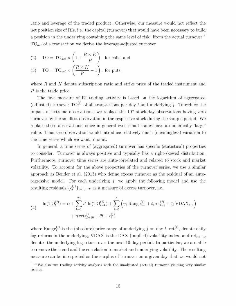
a position in the underlying containing the same level of risk. From the actual turnover15

TOact of a transaction we derive the leverage-adjusted turnover

TO = TOact ×(

1 +R×KP

), for calls, and(2)

TO = TOact ×(R×KP

− 1

), for puts,(3)

where R and K denote subscription ratio and strike price of the traded instrument and

P is the trade price.

The first measure of RI trading activity is based on the logarithm of aggregated

(adjusted) turnover TO(j)t of all transactions per day t and underlying j. To reduce the

impact of extreme observations, we replace the 197 stock-day observations having zero

turnover by the smallest observation in the respective stock during the sample period. We

replace these observations, since in general even small trades have a numerically ’large’

value. Thus zero-observation would introduce relatively much (meaningless) variation to

the time series which we want to omit.

In general, a time series of (aggregated) turnover has specific (statistical) properties

to consider. Turnover is always positive and typically has a right-skewed distribution.

Furthermore, turnover time series are auto-correlated and related to stock and market

volatility. To account for the above properties of the turnover series, we use a similar

approach as Bender et al. (2013) who define excess turnover as the residual of an auto-

regressive model. For each underlying j, we apply the following model and use the

resulting residuals {ε(j)t }t=1,...,T as a measure of excess turnover, i.e.

(4)ln(TO

(j)t ) = α +

20∑k=1

β ln(TO(j)t−k) +

5∑i=0

(γi Range

(j)t−i + δiret

(j)t−i + ζi VDAXt−i

)+ η ret

(j)t,t+10 + θt+ ε

(j)t ,

where Range(j)t is the (absolute) price range of underlying j on day t, ret

(j)t , denote daily

log-returns in the underlying, VDAX is the DAX (implied) volatility index, and rett,t+10

denotes the underlying log-return over the next 10 day period. In particular, we are able

to remove the trend and the correlation to market and underlying volatility. The resulting

measure can be interpreted as the surplus of turnover on a given day that we would not

15We also run trading activity analyses with the unadjusted (actual) turnover yielding very similarresults.

15

have expected based on the model.

Since we want to analyze the positioning (long or short) of RIs in relation to the

direction of TA trading signals, we define a second measure of directional trading activity.

Therefore, we apply the same adjustment as in the first case, but we only aggregate

purchases of calls as long turnover, and purchases of puts as short turnover, respectively.

This means we exclude sell transactions for this consideration because of several reasons.

First, due to the market structure of structured products always requires buying a product

before it can be sold. Thus, the initialization of a long or short trade always requires the

purchase of a call or a put. Second, selling a previously bought instrument can have

several other reasons (e.g. liquidity needs). Even if traders use TA for their trading

decision, they might have to close their position because the original TA signal does not

work as anticipated, although there is no new opposed signal16 Third, because it is also

possible to sell an instrument on another exchange or directly to the issuer, missing sells

could introduce some bias regarding long or short positioning, e.g. investors could prefer

selling calls directly to the issuer. For the directional measure of excess turnover, we use

an adopted vector auto-regression model as follows. Let L(j)t the aggregated turnover of

knock-out calls and call warrants on underlying j bought on day t and analogously S(j)t

put purchases. We define X(j)t = (L

(j)t , S

(j)t )ᵀ and the VAR equation

(5)X

(j)t = α +

5∑k=1

β ln(X(j)t−k) +

5∑i=0

(γi Range

(j)t−i + δiret

(j)t−i + ζi VDAXt−i

)+ η ret

(j)t,t+10 + θt+ ε

(j)t ,

where the variables are in accordance to equation 4, but expanded to two-dimensional

vectors with identical entries. We consider the resulting two-dimensional residuals ε(j)t as

excess long and short turnover and the difference δjt = (1,−1) · ε(j)t of its entries as excess

turnover imbalance which will be used to analyze the positioning of retail investors.

6 Trading Activity

Overall trading activity. To test hypothesis H1a, we consider the overall trading

activity in warrants and knock-outs at Stuttgart stock exchange. Therefore, we employ

the excess turnover time series obtained as the residual of the turnover model (4). In

16For instance, we do not consider pattern confirmations or failures like so-called pull-backs in case ofhead-and-shoulders pattern. Furthermore, we do not check whether a triggered signal is negated whichis usually the case when price break the trigger price levels (e.g. the neckline) in the opposite direction(cf. Bulkowski, 2011). In general, when trading on TA patterns it is not necessarily intended to close aposition only when a signal in the opposite direction occurs, but after a given time or a given price targethas been reached, for example.

16

a first step, we compare the average excess volume on TA signal days and non-signal

days. Additionally we analyze the 3 trading days before and 5 trading days after a signal.

Figure 1 and Table 4 show the differences of (lagged) signal days and non-signal days

to which we apply a t-test (Sattertwaith). Panel A shows the results for pattern signals

and Panel B for moving average signals, respectively. In both cases, we find large excess

turnover on signal days which are significantly different from non-signal days. In case of

pattern signals, this means that on signal days there is about 35% more turnover than

we would have expected. For MA signals this value is about 11%. The smaller impact

of MA signals could indicate a preference for patterns over a long-term MA or that the

clientele for structured products prefers shorter MAs (considered patterns evolve mostly

over less than two months) as their trading activities tend to have a shorter horizon.

Insert Figure 1 here.

Insert Table 4 here.

Considering the days before and after a signal, we find negative differences, i.e. negative

excess turnover two days before a pattern signal. This could indicate that RI using TA

wait for the triggering of a pattern after the last relevant extremum has emerged. Note

that this difference is only significant on the 5% level due to the relatively large deviation.

Similarly, MA signals exhibit a reversal in excess volume two days after a signal occurred

as well as positive excess turnover 4 days after the signal which is of smaller magnitude

than on the signal day, however. This might also be a result of the combination of MAs

which often have slightly shifted trigger days or varying individual filter criteria applied

in practice. Assuming that not all RIs are day traders or are trading each day, the lagged

observation17 of a TA signal could result in increased excess volume multiple days after

an event.

In a second step, we apply a panel regression analysis to confirm the descriptive

evidence. Therefore, we estimate the following regression for the excess turnover, i.e.

the residuals ε(j)t obtained from model (4).

ε(j)t = α + β ∗ Psig(j)t + γ ∗MAsig

(j)t + ξ

(j)t ,(6)

where Psig(j)t and MAsig

(j)t equal 1 if a TA and MA signal occurred in underlying j

on day t or are zero, else. Note that, we do not include firm dummies since the input

excess turnover series was estimated per firm and the resulting residuals have zero mean.

Consequently the intercept is not significant. However, the variance of those models

17Lo et al. (2000, p.1719) use a 3-day lag to ”control for the fact that in practice we do not observe arealization [...] as soon as it has completed”.

17

estimated per stock can differ in general. Thus we use Thompson (2011) clustered

standard errors which cluster in time (day) and stock as well as in the intersection.

Estimation results are shown in Table 5, column (1). Confirming the descriptive test,

both signal types have a significant and positive effect on excess turnover at Stuttgart

stock exchange. Naturally, R-squares are very low for these regressions as most of the

explainable variation is already absorbed by the preceding models (4) or (5). Furthermore,

signals are in general a quite rare event (about 6% of stock days) and can therefore not

explain much of the overall variation. Despite that, the model confirms the large impact

of a triggered trading signal on excess turnover. When we extend equation (4) by an

additional interaction term of MA and pattern signal indicators, Column (2) shows that

this effect is not significant. In general this is an extremely rare event18 in our data.

Insert Table 5 here.

Alternatively to the two-step approach, we could also combine models (4) and (6) to esti-

mate the normalization and TA signal effects simultaneously. Although the interpretation

regarding the parameters used for the validation of hypothesis H1 remain unchanged, we

prefer the two-step approach as the statistically more sound way to obtain this results.

This is basically because we allow the impacts of variables used in model (4) to be

stock specific and independent of potential effects from TA signals. Indeed, we do not

account for cross-sectional effects or industry effects and only account for market volatility

measured by VDAX index. The estimation results from the full model add no further

insights19 and are less consistent to analyze the hypothesized effect (H1a) since the two-

step approach measures the effect with respect to the turnover that would have been

expected from contemporaneous and lagged trading variables.

To differentiate between the considered pattern and moving average types, we adapt

the regression model by including dummies for each considered pattern and MA type.

Estimation results are reported in Table 5, column (3). Double Tops and Bottoms and

(Inverse) Head and Shoulder patterns have the largest impact on excess turnover while

both are statistically significant. The estimated effect of rectangle tops and bottoms

is positive but not significant. This could indicate a more ambiguous definition of this

pattern type or that the pattern is not as popular as the two previous ones. For moving

average type signals similar results emerge. The SMA200 (with 0,1% filter) can be

associated with a 20% increase in excess turnover which is highly significant on a 0.1%

confidence level. However, both crossover MA types show values close to zero. This might

be due to the more subjective implementation of double moving averages. While the 200-

day SMA is quite unique, the shorter MA of the dual MA strategy could be applied with

18Only on 36 stock-days a pattern and MA signal is triggered simultaneously.19Thus, results are not printed but can be made available on request.

18

basically any length. This could dilute the time of observation we consider and could also

mean that the turnover based on these strategies is distributed over multiple days. We

also tested DSMA10/100 and DSMA20/200 with very similar regression results. Hence,

we drop the dual DSMA signals for the remainder of this paper.

Positioning. With respect to hypothesis H1b, we consider the excess turnover long-

short imbalance obtained from regression (5). We apply two regression models similar

to model (6). In the first model we use two dummy variables which equal one if any

buy (sell) signal in an underlying occurred on day t. For the second model, we use

all long and short signal of head and shoulder, double top and bottom, and rectangle

top & bottom pattern, as well as the 200-day simple moving average, i.e. eight signal

dummy variables in total. Results are reported in Table 6. Both models do not support

hypothesis H1b. For the first model, reported in column (1), estimated coefficients of buy

signal and sell signal dummies are not significant and close to zero but the signs are in the

expected direction. The second model, reported in column (2), shows that the estimates

for individual trading signals neither have a significant impact on turnover imbalances on

a 10 % level. Note that, we only consider call buys and put buys, respectively, i.e. there

are no direct reversal effects from selling positions which could be considered as long or

short positioning and thus might affect the model results in any direction. A possible

explanations for the results on excess turnover imbalances could be that only a subgroup

of RI use TA while another group acts in the opposite direction. Since TA signals always

appear after a price movement in the same direction20 of the signal, contrarian trading

usually is opposed to TA based trading. Overall, hypothesis H1b must be rejected in the

sense that TA signals cannot reliably predict (net) positioning of RIs measured by daily

(excess) trading imbalances.

Insert Table 6 here.

7 Trading Characteristics

In addition to the aggregated trading activity in structured products at Stuttgart Stock

Exchange, we now focus on trade characteristics of round-trip trades. Therefore, we use

the sample of matched trades described in Section 4. For each round-trip trade i we

calculate three return measures, i.e. log-return ri, risk-adjusted return radji , and risk-

20I.e. price increase for a buy signal and price decrease for a sell signal, respectively.

19

adjusted excess return radjexi defined as

ri = 100 ∗ log

(Psell

Pbuy

)radji = 100 ∗ log

(P selli

P buyi

)/ (L ∗ σi))

radjexi =

100 ∗(

log(

P selli

P buyi

)− log

(Uselli

Ubuyi

))/ (Li ∗ σi) , for calls

100 ∗(

log(

P selli

P buyi

)+ log

(Uselli

Ubuyi

))/ (Li ∗ σi) , for puts

where P buy (P sell) denotes the buying (selling21) price, U buyi (U sell

i ) the price of the under-

lying at purchase (sale), Li is the leverage of the traded product at purchase as defined in

equation (2), and σi denotes the annualized 20-day volatility of the underlying. We use the

historical volatility to account for the risk involved since realized volatility calculated over

the holding period often behaves erratically, in particular for very short trading horizons

like a couple of hours.

Insert Figure 2 here.

Figure 2 depicts the empirical distributions of leverage, holding period, and log-returns

of the whole sample. The high leverage ratio incorporated in the traded instruments

highlights the highly speculative character of these trades. Since the population of RI

are considered to be uninformed noise traders (cf. Meyer et al., 2014), gambling and

entertainment seem to be a major incentive for trading KOs and warrants. The holding

duration supports the consideration of this trades (and products) as short-term bets.

The median holding period is less than two days, i.e. most trades are completed within

one or two days22. The numbers regarding earned returns are quite devastating for RI

trading KOs and warrants. On average, a trade loses about 4% of the invested capital.

Interestingly, the median log-return is positive, i.e. the log-return distribution is highly

skewed to the left. RI realize profits more often, but also realize extreme losses which

in many cases means the total invested capital. Approximately 7.48% of the trades

considered are knocked-out or expire worthless. These descriptive facts are an indication

for the presence of the disposition effect for RI trading structured products which confirms

several existing studies on RIs (see Section 2.1).

21As described in Section 5, we use a selling price of 1 cent if a product is knocked-out and the innervalue of the product if it expires.

22Note that the histogram is cut off after 30 days, although the maximum trade duration consideredis one year. Generally there are also long-term trades which the much larger mean (about 14 days) incomparison to the median indicates.

20

To assess research question RQ2, we analyze whether there are differences between

trades that have been entered on days of a TA trading signal. To achieve this, we

use trading signals generated by the three pattern types and the SMA200. We define

the dummy variables buysigi and sellsigi which equal one if a buy signal and a sell

signal, respectively, occurred on the day on which round-trip trade i was entered. To test

whether there are significant drivers of round-trip trade returns, we estimate the following

linear regression with double-clustered standard errors (Thompson (2011), Cameron et al.

(2011)).

ri =β1 ∗ buysigi ∗ ci + β2 ∗ buysigi ∗ pi + γ1 ∗ sellsigi ∗ ci + γ2 ∗ sellsigi ∗ pi(7)

+ δ1 ∗ holdingi ∗ ci + δ2 ∗ holdingi ∗ pi + η ∗marketi + ζ ∗ koi + controls+ εi,

where ci and pi are dummy variables for call and put, holdingi denotes the duration of

trade i in days, marketi is a dummy for market buy order, and koi indicates trades in

knock-out products. The term controls is defined as∑

j

(ul

(j)i ∗ ci + ul

(j)i ∗ pi

), where

dummy ul(j)i equals 1 if the underlying of tradei is j. This means we have fixed effects

for each underlying and trade direction (i.e. long or short trades) in terms of call or put

products. Thus we evaluate whether trade performance varies within the peer group of

products on the same underlying and of the same option type but assume that the effects

regarding TA trading signals are related across all groups. This is necessary because puts

and calls on the same underlying generally behave diametrically23. Since the expected

effects of trading signals on performance are opposed for puts and calls, we use separate

dummies for buy signals and sell signals, respectively.

Insert Table 7 here.

For the three return measures defined above we report the estimation results in Table 7.

The model indicates that round-trip trades which are entered on days of TA buy signals

and are in accordance to those signals, i.e. call products, earn higher (raw) log-returns,

while put trades earn lower returns (see column 1) on these signal days. Parameter β1 and

β2 show that these trades have 8.27% higher resp. 13.99% lower (log-) returns and both

estimates are significant on a 1% level. Note that the abnormal returns estimated by the

parameter coefficients are with respect to other trades on the same underlying and option

type. This does not mean that these trades must have been profitable at all, but at least

23In case the underlying price does not change while the underlying volatility increases or timeprogresses, both, put and call prices could increase or decrease. However, due to the large numberof trades and the long observation period such special cases can be neglected here. Alternatively, wecould estimate the model for puts and calls separately but then it is not possible to distinguish whetherall trades were profitable on buy (sell) signal days or just calls (puts).

21

have been less unprofitable than comparable trades. Analogously, trades entered on sell

signal days tend to have better performance for puts and weaker performance for calls.

The estimates indicate an impact on log-returns of 5.23% for puts and -3.23% for calls,

thus the effect is of smaller magnitude than in the buy signal case, but still significant on

a 1% level.

Considering risk-adjusted returns, we observe the same effect in case of buy signals.

Naturally, the parameter estimates are smaller since dividing by leverage and volatility

dampens the return values. If a call trade is entered on a buy signal, there is a positive

effect on performance of 1.11% while puts earn 1.97% less. For sell signals the estimates

differ from the non-adjusted case. While calls do not earn significantly differing risk-

adjusted returns compared to the remaining trades, puts even show worse performance

than puts on non-signal trades and on the same underlying. This could mean that puts

on signal days buy the extra return from increased risk. So it might be the case that

the results regarding raw returns of puts bought on sell signal days are driven by some

very successful trades which use very high leverage. For risk-adjusted excess returns we

basically get a similar result as for risk-adjusted returns. Here, estimates are very small as

most variation is absorbed by the standardization. Since the return of a KO or warrant

is (to a large extend) a function of the return of the underlying and the incorporated

leverage, the standardized excess return mainly consists of time-dependent and non-linear

components of the price and mispricing which includes product premia and other costs,

for example. The estimates indicate that for this remaining part of the return, effects are

close to the risk-adjusted case, i.e. a significant positive (negative) effect for calls (puts)

on buy signal days, and no effect in case of sell signals.

Other trade characteristics affecting the performance of a round-trip trade turn out

to be as expected. A longer holding duration has a negative impact on returns, likely

due to the inner costs of structured products. Not surprisingly, market orders also imply

lower returns since RI have to pay the spread24 in this case. If we do not adjust for

leverage, there is no significant difference between knock-outs and warrants. In case of

risk-adjustment, knock-outs earn higher (risk-adjusted) returns since these trades show

less leverage. On the other hand, price changes are more affected by leverage in case of

knock-outs compared to warrants25.

To check whether differences in realized returns can also be found in other trade

characteristics, we consider the (log) leverage at purchase and the holding period of a

24Our return measures always include spread costs (if applicable) and do not consider exchange fees orother costs. Spreads are usually fixed by the market maker and issuing bank on a specific level (typicallyEUR 0.01) which can have a major impact on returns for low-price products.

25Since the option delta of warrants is smaller than one, prices do not change as much if the leverageof both products is equal.

22

trade. We run a regression model similar to (7) where we only use variables which are

known at the time of the independent variable observation. Thus terms containing the

holding period are not regressed on leverage (at purchase). We also add terms for the

underlying’s volatility (at purchase). In case of holding duration, we only control for

underlying and use a single call product dummy instead of one for each underlying. The

estimation results are reported in Table 8.

Insert Table 8 here.

General effects on the leverage of the product at purchase tend to be as expected. Higher

underlying volatility leads to less leverage in the selected product as the underlying itself

tends to be more risky. With respect to TA signals, the results confirm the interpretations

regarding regression model (7) applied to risk-adjusted returns. Call round-trip trades

on buy-signal days do not incorporate higher leverage which could explain the positive

effect on performance, but even tend to involve less leverage. An analogous interpretation

holds in case of puts. That is, in those trades which are in accordance to TA signals, RIs

have chosen less leverage compared to trades on the same underlying and option type on

non-signal days.

For the duration of round-trip trades we find that call trades initiated on buy signal

days and put trades on sell signal days tend to be sold sooner compared to their benchmark

group. Although a longer holding period is generally costly due to the inner costs of a

structured product and therefore does influence the performance of a trade (for which

we control in model (7)), the favorable (unfavorable) performance of trades probably

influences the holding duration when RI are affected by the disposition effect. Since we

have no subject-level information it is impossible to disentangle the inter-dependencies

between (current) performance of the trade, holding duration (i.e. the decision to close a

position), and the disposition effect of a RI.

Insert Figure 3 here.

In the above models, we considered the trading performance (and other characteristics)

of round-trip trades, i.e. purchases of puts and calls on days of a TA buy and sell

signal, respectively, and on days when no signal occurred. The regression models show

that there are differences in the means of the considered groups of trades. Now we also

want to investigate potential differences in the total return distribution. Figure 3 shows

the (de-meaned) empirical distributions of round-trip trades in calls and puts on signal,

and no-signal days, respectively. For the upper plot buy signals are considered and for

the bottom plot sell signals, respectively. In case of buy signals, we see quite different

shapes of the empirical distribution. Call trades, which would be in line with TA-based

23

trading, show less extreme and more symmetric returns around the mean compared to

call trades on non-signal days. In case of puts the difference is even more evident. Put

trades entered on buy signal days have a very long left tail and generally more extreme

returns compared to put trades on non-buy-signal days. To assess the differences in the

shape and the higher moments of the return distributions we run two tests. First, we use

a two-sample Kolmogorov-Smirnov test on the standardized26 (by mean and standard-

deviation) return distributions and compare call (put) trades on buy (sell) signal days

compared to the other groups. The test results shown in column 3 of Table 9 confirm

that the considered return distributions are significantly different on a 0.1% level. This

means the return distributions have statistically significant differences in their higher

moments. Since we are particularly interested in the skewness of the realized returns, we

calculate the Bowley coefficient sB and Groeneveld and Meeden (1984) skewness measure

sGM . For a random variable X with mean µX , median νX , and quartiles Qi, i = 1, 2, 3,

these measures are defined by

sB =Q3 +Q1 − 2Q2

Q3 −Q1

sGM =µX − νX

E|X − νX |.

We do not use the standard sample skewness since it is not robust to outliers and fat-tailed

distributions which here is the case (cf. Groeneveld and Meeden, 1984). To test whether

the skewness measures can be (statistically) distinguished between two sets of round-trip

trades, we construct confidence levels from a resampling procedure. Therefore, we pool the

observation from both samples and randomly draw two new sets having the same size as

the original ones. For the sampled sets we calculate the absolute difference of the skewness

measures. We run 100,000 repetitions to obtain the distribution of this difference from

which we derive the 0.1% confidence levels. Panel A of Table 9 shows the results for buy

signals while for Panel B presents results for sell signals. The corresponding confidence

levels for the absolute difference of the skewness measures are reported in parentheses.

For buy signals (Panel A), we find that the return distribution of calls bought on signal

days is less left-skewed (sB = −0.1049, sGM = 0.1993) than the return distributions of

other groups which is significant on a 0.1% level in all cases. Puts bought on buy signal

days (i.e. opposed to trade direction of the TA signal) exhibit the most left-skewed return

distribution (sB = −0.4482, sGM = −0.3825). A reason for this might be that signal

triggers are associated with short-term momentum since the signals require a (preceding)

26We also run Kolmogorov-Smirnov tests on the original and centered distribution, both resulting inrejection of the null in all pairwise comparisons.

24

price movement in the direction of the signal. The opposite trade could then suffer from

this short-term momentum, but the high leverage and the risk to be knocked-out can

quickly lead to an undesirable situation for the investor where she must sell the position

with a big loss. If we assume that traders prefer right-skewed returns, then traders who

follow TA signals in our sample actually achieve this. The latter is in accordance to the

simulation result of Ebert and Hilpert (2013). Furthermore the tendency to realize less

left-skewed returns indicates that RI who use TA-based strategies are less prone to the

disposition effect. Using a static rule or another systematic approach might reduce the

risk to be influenced by behavioral biases as the decision of closing a trading position is

given by the applied TA strategy or some other trading rule.

Insert Table 9 here.

For sell signals (Panel B) it turns out that call trades exhibit less left-skewed returns

than trades in put products. A reason might be the generally worse performance of

put round-trip trades which to a large extent is due to the strong market recovery

during the observation period27. Thus, a randomly entered put trade was usually an

unfavorable bet with a high chance that the investor’s position falls below the purchase

price. Consequently, these trades are more often faced with a big loss which traders who

are prone to the disposition effect are reluctant to realize, but eventually the trade ended

up even worse. Comparing put trades entered on sell signal and non-signal days, shows

that the skewness measure are sB − 0.1092 (sGM = −0.3035) for the signal group and

sB − 0.2739 (sGM = −0.3628) for the non-signal which is significantly different on 0.1%

level. So for both, buy signals and sell signals, we can confirm hypothesis H2b, i.e. trades

in accordance to the respective trading signals are less (left-)skewed than trades in the

same direction on non-signal days. In this sense, TA traders could be more disciplined in

their trading effort and realize losses sooner.

8 Conclusion

In this study, we have explored the relation between TA and trading on a RI-dedicated

market. Based on a set of trading signals from typical TA techniques, chart patterns and

moving averages, we have addressed two main research questions regarding the influence of

TA on trading (cf. Section 3). How do TA-based strategies and the corresponding trading

signals influence trading activity[...] (RQ1) and which are the characteristics of trades

that have been initiated in accordance to TA trading signals[...] (RQ2). With respect to

27The DAX rose from 4075 on April 1, 2009 to 9552 at the end of 2013, that is an increase of about134% in less than five years.

25

RQ1, we find that overall trading activity is substantially increased on TA signal days. A

pattern signal from the three considered pattern types is associated with a 35% increase in

excess turnover, on average. Regression results show that Head & Shoulders and Double

Tops & Bottoms have a particularly strong impact on market activity. For MA signals

an increase of 11% is observed. This means, trading activity in speculative structured

products is related to TA signals. However, our analysis of (long-short) excess trading

imbalances of RI reveals that there is no significant (positive or negative) relation between

trading signal direction and the positioning of RI. This might be due to other attention

effects which influence RIs and their trading behavior. For example, on an intraday level

the increased turnover could initially induce attention and thereby attract more traders

who tend to trade in a contrarian way, i.e. opposed to the TA signal. Then, we would

find increased excess turnover on this day, but no reliable explanation for the exposure

in the direction of the TA signal. Unfortunately, the sparsity of RI trading activity in

products on a specific stock and the generally fuzzy observation of TA signals does not

allow for a higher time granularity on a reasonable basis.

Regarding RQ2 we find that the trade characteristics of round-trip trades which

were initiated in accordance to the direction of TA trading signals (i.e. long or short)

do remarkably differ from round-trip trades on the same underlying and in the same

direction. In terms of raw returns, these trades tend to perform significantly better than

comparable trades on non-signal days. Based on our analyses it is hardly possible to

infer the origin of the improved performance. We share the view of previous studies that

TA as a systematic trading strategy is not able to earn consistent above-market returns

(net of transaction costs). Yet, the exploitation of short-term momentum (maybe even

induced by the increased attention itself) might play a role and could lead to increased

returns for a limited period of time. Furthermore we find that the return distribution of

trades in accordance to TA trading signals differ in the shape of their return distribution.

Round-trip trades in calls on buy signal days, and puts on sell signal days, respectively,

are less left-skewed than their peers. Using a resampling methodology, these differences

turn out to be not by chance (on a 0.1% level). This can be interpreted as a reduced

propensity to the disposition effect, i.e. realizing gains earlier than losses which would

result in a left-skewed return distribution. Another interpretation of this result is that

TA addresses the gambling and entertainment aspects of trading and is used by traders to

place their bets. Indeed, the effect of TA strategies to skew the realized return distribution

to the right has been found theoretically (Ebert and Hilpert, 2013) and is confirmed in

our study empirically based on the distribution of realized returns of the considered trades

on Stuttgart Stock Exchange. In addition to performance, other trade characteristics are

found to differ for TA-related round-trip trades. They tend to be of shorter duration and

26

contain less leverage at the time of purchase. Both findings confirm the view that TA

changes typical trade characteristics of RIs.

Our results are limited with respect to the assumptions made. We apply a relatively

narrow set of TA strategies which we assume to be relevant based on the literature and

our view on practice, for example in financial media, TA handbooks or trading blogs. The

calibration of the patterns and MAs is somewhat subjective, however the consideration

of daily observations might offset some of the fuzziness regarding the exact triggering of

a signal. It is also possible that the relative narrow set of MAs and the fixed pattern

calibration do not include the most typical calibration of MA and patterns which RI

trading structured products are using. Yet we believe that searching (fitting) the TA

method yielding the ”highest” result would not have been a sensible approach in our

case. With respect to the trading data from Stuttgart Stock Exchange, we are limited

by the fact that we can observe trading only on a population level, i.e. no individual

trading information is available. Therefore, we cannot conclude that the observed effects

are consistent in the sense that some trader who trades on a signal actually has traded

on that signal and also will do so on a future signal of that (and only that) kind. A

complementary survey28 among trading participants could be an interesting extension to

shed light on the trading incentives of RI trading at Stuttgart Stock Exchange.

If we conclude that RI use TA, like our study is indicating, the question arises why

people actually use TA. Does the use of TA and the related trading just entertain investors

- hence it had a value in itself - or does the lack of investment knowledge and the demand

for a guiding system for making (profitable) investment decisions play a dominant role?

If the latter is true, many offers by brokers and information providers excessively praising

chart and TA tools should be considered critically. Therefore, the way TA, charts, and

other related methods influence trading decisions of investors is an important question

which we leave for future research.

28Similar to the approach of Hoffmann and Shefrin (2014) who use a survey to identify the investmentstyle of broker clients.

27

References

Bajgrowicz, P. and O. Scaillet (2012): “Technical trading revisited: False

discoveries, persistence tests, and transaction costs,” Journal of Financial Economics.

Barber, B. M., Y.-T. Lee, Y.-J. Liu, and T. Odean (2014): “The cross-section of

speculator skill: Evidence from day trading,” Journal of Financial Markets, 18, 1–24.

Barber, B. M. and T. Odean (2000): “Trading is Hazardous to Your Wealth:

The Common Stock Investment Performance of Individual Investors,” The Journal

of Finance, 55, 773–806.

——— (2007): “All That Glitters: The Effect of Attention and News on the Buying

Behavior of Individual and Institutional Investors,” Review of Financial Studies, 21,

785–818.

——— (2011): “The behavior of individual investors,” Available at SSRN 1872211.

Barber, B. M., T. Odean, and N. Zhu (2008): “Do Retail Trades Move Markets?”

Review of Financial Studies, 22, 151–186.

——— (2009): “Systematic noise,” Journal of Financial Markets, 12, 547–569.

Bauer, R., M. Cosemans, and P. Eichholtz (2009): “Option trading and individual

investor performance,” Journal of Banking and Finance, 33, 731–746.

Benamar, H. (2013): “To See is To Know: Efficient Display of Market Data for Retail

Investors,” eurofidai.org.

Bender, J. C., C. L. Osler, and D. Simon (2013): “Noise Trading and Illusory

Correlations in US Equity Markets,” Review of Finance, 17, 625–652.

Blume, L., D. Easley, and M. O’hara (1994): “Market statistics and technical

analysis: The role of volume,” The Journal of Finance, 49, 153–181.

Brock, W., J. Lakonishok, and B. LeBaron (1992): “Simple technical trading rules

and the stochastic properties of stock returns,” The Journal of Finance, 47, 1731–1764.

Bulkowski, T. N. (2011): Encyclopedia of chart patterns, vol. 225, John Wiley & Sons.

Cameron, a. C., J. B. Gelbach, and D. L. Miller (2011): “Robust Inference With

Multiway Clustering,” Journal of Business & Economic Statistics, 29, 238–249.

28

Daniel, K., K. Daniel, D. Hirshleifer, D. Hirshleifer, A. Subrahmanyam,

and A. Subrahmanyam (1998): “Investor psychology and investor security market

under-and overreactions,” Journal of Finance, 53, 1839–1886.

Dhar, R. and A. Kumar (2001): “A non-random walk down the main street: Impact

of price trends on trading decisions of individual investors,” Yale International Center

for Finance. Working Paper.

Dhar, R. and N. Zhu (2006): “Up Close and Personal: Investor Sophistication and

the Disposition Effect,” 52, 726–740.

Dorn, D. and P. Sengmueller (2009): “Trading as Entertainment?” Management

Science, 55, 591–603.

Ebert, S. and C. Hilpert (2013): “The Trend is Your (Imaginary) Friend: A

Behavioral Perspective on Technical Analysis,” Available at SSRN 2354962, 31.

Engelberg, J., C. Sasseville, and J. Williams (2011): “Market Madness? The

Case of Mad Money,” Management Science, 58, 351–364.

Entrop, O., M. McKenzie, M. Wilkens, and C. Winkler (2014): “The

performance of individual investors in structured financial products,” Review of

Quantitative Finance and Accounting.

Etheber, T. (2014): “Trading Volume Effects of Moving Average Heuristics,” Available

at SSRN 2517005.

Etheber, T., A. Hackethal, and S. Meyer (2014): “Trading on Noise: Moving

Average Trading Heuristics and Private Investors,” Available at SSRN 2520346, 49.

Flanegin, F. and D. Rudd (2005): “Should investments professors join the crowd,”

Managerial Finance, 31.

Fritz, F. and S. Meyer (2012): “Pricing of Bank-Issued Investment Products-

Premium Shifts and Investor Wealth,” Available at SSRN 2153723.

Glaser, M., T. Langer, and M. Weber (2007): “On the Trend Recognition and

Forecasting Ability of Professional Traders,” Decision Analysis, 4, 176–193.

Glaser, M. and M. Weber (2004): “Overconfidence and Trading Volume,” M.

Goetzmann, W. N. and A. Kumar (2008): “Equity portfolio diversification,” Review

of Finance, 12, 433–463.

29

Graham, J. R. and A. Kumar (2006): “Do dividend clienteles exist? Evidence on

dividend preferences of retail investors,” Journal of Finance, 61, 1305–1336.

Grinblatt, M. and M. Keloharju (2000): “The investment behavior and perfor-

mance of various investor types : a study of Finland ’ s unique data set,” Journal of

Financial Economics, 55, 43–67.

——— (2009): “Sensation seeking, overconfidence, and trading activity,” Journal of

Finance, 64, 549–578.

Grinblatt, M., M. Keloharju, and J. T. Linnainmaa (2012): “IQ, trading

behavior, and performance,” Journal of Financial Economics, 104, 339–362.

Groeneveld, R. a. and G. Meeden (1984): “Measuring skewness and kurtosis,”

Journal of the Royal Statistical Society. Series D (The Statistician), 33, 391–399.

Han, B. and A. Kumar (2013): “Speculative Retail Trading and Asset Prices,” Journal

of Financial and Quantitative Analysis, 48, 377–404.

Hoffmann, A. O. and H. Shefrin (2014): “Technical analysis and individual

investors,” Journal of Economic Behavior & Organization.

James, F. E. (1968): “Monthly Moving AveragesAn Effective Investment Tool?” Journal

of Financial and Quantitative Analysis, 3, 315–326.

Jensen, M. and G. Benington (1970): “Random walks and technical theories: Some

additional evidence,” The Journal of Finance, 25, 469–482.

Kavajecz, K. a. and E. Odders-White (2004): “Technical Analysis and Liquidity

Provision,” Review of Financial Studies, 17, 1043–1071.

Keloharju, M., S. Knupfer, and J. Linnainmaa (2012): “Do Investors Buy What

They Know? Product Market Choices and Investment Decisions,” Review of Financial

Studies, 25, 2921–2958.

Kirkpatrick II, C. D. and J. Dahlquist (2012): Technical analysis: the complete

resource for financial market technicians, FT press.

Kumar, A. and C. Lee (2006): “Retail investor sentiment and return comovements,”

The Journal of Finance, 61, 2451–2486.

Lease, R. C., W. G. Lewellen, and G. G. Schlarbaum (1974): “The individual

investor: attributes and attitudes.” The Journal of Finance, 29, 413–433.

30

Lo, A., H. Mamaysky, and J. Wang (2000): “Foundations of technical analysis:

Computational algorithms, statistical inference, and empirical implementation,” The

Journal of Finance, 55.

Menkhoff, L. (2010): “The use of technical analysis by fund managers: International

evidence,” Journal of Banking & Finance, 34, 2573–2586.

Menkhoff, L. and M. Taylor (2007): “The obstinate passion of foreign exchange

professionals: technical analysis,” Journal of Economic Literature, 45, 936–972.

Meyer, S., S. Schroff, and C. Weinhardt (2014): “(Un)skilled leveraged trading

of retail investors,” Financial Markets and Portfolio Management, 28, 111–138.

Neuhierl, A. and B. Schlusche (2011): “Data snooping and market-timing rule

performance,” Journal of Financial Econometrics, 9, 550–587.

Odean, T. (1998a): “Are Investors Reluctant to Realise their Losses?” The Journal of

Finance, 53, 1775–1798.

——— (1998b): “Volume , Volatility , Price , and Profit When All Traders Are Above

Average,” The Journal of Finance, 53, 1887–1934.

Osler, C. (2003): “Currency orders and exchange rate dynamics: an explanation for the

predictive success of technical analysis,” The Journal of Finance, LVIII, 1791–1819.

Osler, C. L. (2000): “Support for resistance: technical analysis and intraday exchange

rates,” Economic Policy Review, 53–68.

Park, C.-H. and S. H. Irwin (2007): “What Do We Know About the Profitability of

Technical Analysis?” Journal of Economic Surveys, 21, 786–826.

Savin, G., P. Weller, and J. Zvingelis (2006): “The Predictive Power of ”Head-

and-Shoulders” Price Patterns in the U.S. Stock Market,” Journal of Financial

Econometrics, 5, 243–265.

Schmitz, P. and M. Weber (2012): “Buying and selling behavior of individual

investors in option-like securities,” DBW-Die Betriebswirtschaft.

Schroff, S., S. Meyer, and H. Burghof (2013): “Individual Investor Trading in

Leverage Products-Risk Appetite and Positioning Around Earnings Announcements,”

Available at SSRN 2223957.

31

Seasholes, M. S. and G. Wu (2007): “Predictable behavior, profits, and attention,”

Journal of Empirical Finance, 14, 590–610.

Shefrin, H. and M. Statman (1985): “The Disposition to Sell Winners Too Early and

Ride Losers Too Long: Theory and Evidence,” The Journal of Finance, 40, 777–790.

Stoimenov, P. a. and S. Wilkens (2005): “Are structured products fairly priced?

An analysis of the German market for equity-linked instruments,” Journal of Banking

& Finance, 29, 2971–2993.

Subrahmanyam, A. (2008): “Behavioural finance: A review and synthesis,” European

Financial Management, 14, 12–29.

Thompson, S. B. (2011): “Simple formulas for standard errors that cluster by both firm

and time,” Journal of Financial Economics, 99, 1–10.

Wilkens, S., C. Erner, and K. Roder (2003): “The Pricing of Structured Products

in Germany,” 11, 55–69.

32

Tables and Figures

Figure 1: Excess trading on TA signal days.

The figures depict excess turnover in structured product at Stuttgart Stock Exchange from three daysbefore to 5 days after a TA signal occurred in the respective underlying. The top and bottom plot arebased on signals by chart patterns signals and moving average signals, respectively.

33

Table 1:Descriptive Statistics of Trading Data from Stuttgart Stock Exchange.

Key facts of trade data from Stuttgart Stock Exchange. The sample contains all trades in DAX andDAX30 warrants and knock-outs from 2009/04/01 to 2013/12/31. The matching rate refers to the shareof buy transactions that can be matched by the algorithm described in section 5. From the resultingsample of round-trip trades, trades below EUR 0.1 or completed in less than two minutes are deleted.

Overall Knock-Outs WarrantsCalls Puts Calls Puts

# Instruments 266,783 62,408 47,466 96,827 60,082# Trades (mn) 3.6950 0.7647 0.9292 1.2330 0.7680# Buys (mn) 1.9761 0.3753 0.4611 0.6974 0.4424# Sells (mn) 1.7189 0.3894 0.4681 0.5357 0.3256Total Turnover (mnEUR) 15.2376 2.1885 2.5711 6.7007 3.7773Buy Turnover (mnEUR) 7.6444 1.0264 1.2414 3.3844 1.9922Sell Turnover (mnEUR) 7.5932 1.1621 1.3297 3.3163 1.7851Avg. Trade Size (EUR) 3,995 2,862 2,767 5,434 4,918Avg. Time to maturity (d), buys only 129 60 92 234 131Matching rate 58.1% 72.1% 71.9% 47.8% 49.8%Round-trip trades (mn) 1.0853

Table 2: Technical analysis trading signals in DAX and DAX30 stocks.

Trading Signals in DAX and DAX30 stocks from May 2009 to November 2013 (1209 trading days)generated by the technical analysis algorithms introduced in section 5

.Event type Overall signals Signals per stock/day Buy signals Sell signals

(Inverse) Head-and-Shoulders 327 0.87% 172 155Double Top & Bottom 100 0.27% 48 52Rectangle Top & Bottom 102 0.27% 56 46SMA 200 (0.1% filter) 979 2.61% 499 480Dual SMA-20-100 522 1.39% 265 257Dual SMA-50-200 208 0.55% 117 91

Overall 2238 5.97% 1157 1081

Table 3: Comparison of pattern recognition calibration.

This table compares TA signal generated from different calibrations of the smoothing factor h of theKernel regression. The first block contains recognition results from h determined by cross-validation withmultiplier 3. The second and third block show results from constant h = 1.0, and h = 1.5, respectively.Row (1), (2), and (3) show details on the recognition of (Inverse) Head-and-Shoulders, Double Top &Bottom, and Rectangle Top & Bottom, respectively. For each calibration the total number of signalsfound and the absolute and relative number of signals matching the signals of the main calibration(h = 1 + 8σi, where σi denotes the standard deviation of the price differences in window i) are reported.

cross-validation, h-multiplier=3.0 constant h=1.0 constant h=1.5

matches matches matches# signals abs. rel. # signals abs. rel. # signals abs. rel.

(1) 277 160 57.76% 361 281 85.93% 178 127 71.35%(2) 89 58 65.17% 97 92 94.85% 116 77 77.00%(3) 99 49 49.49% 128 96 94.12% 51 43 84.31%

34

Table 4: Excess trading turnover on TA signal days.

Trading Signals in DAX and DAX30 stocks from May 2009 to November 2013 (1209 trading days)generated by the technical analysis algorithms introduced in section 5

Panel A: Pattern signal

Lag No signal Signal Diff Ttstat p-value-3 0.0018 -0.0272 -0.0290 -0.63 0.5260-2 0.0037 -0.1327 -0.1364 -2.50 0.0125-1 0.0010 0.0098 0.0088 0.18 0.85690 -0.0050 0.3018 0.3068 7.19 0.00011 0.0031 -0.0816 -0.0847 0.65 0.51752 0.0006 0.0236 0.0230 0.15 0.87783 0.0019 -0.0435 -0.0454 -0.90 0.36794 0.0006 0.0080 0.0074 0.46 0.64305 0.0004 0.0307 0.0303 -1.66 0.0982

Panel B: Moving Average Signal

Lag No signal Signal Diff Ttstat p-value-3 -0.0011 0.0382 0.0393 1.21 0.2253-2 0.0001 0.0003 0.0002 0.01 0.9946-1 0.0016 -0.0300 -0.0316 -0.94 0.34990 -0.0039 0.1082 0.1121 3.91 0.00011 0.0009 0.0056 0.0047 -0.27 0.78832 0.0045 -0.0862 -0.0907 1.99 0.04633 0.0021 -0.0252 -0.0273 -0.86 0.39254 -0.0014 0.0580 0.0594 -2.61 0.00915 0.0009 -0.0085 -0.0093 0.14 0.8895

35

Table 5: Excess trading turnover regressed on TA signal indicators.

Column (1) presents estimation results from the regression ε(j)t = α+ β ∗ Psig(j)t + γ ∗MAsig

(j)t + ξ

(j)t ,

where ε(j)t is the excess turnover in stock j on day t, Psig

(j)t and MAsig

(j)t equal 1 if a TA and MA signal

occurred in underlying j on day t or are zero, else. We use Thompson (2011) (double) clustered standarderrors. In column (2) the model contains an interaction term of pattern and MA-event indicators and forcolumn (3) each pattern and MA-type is used as a separate dummy. *, **, and *** denote significanceon the 5%, 1%, and 0.1% level, respectively.

Excess Turnover(1) (2) (3)

Estimate Std. Error Estimate Std. Error Estimate Std. Error

Intercept -0.0101 0.0070 -0.0103 0.0070 -0.007 0.0071Pattern signal 0.3012*** 0.0443 0.3106*** 0.0466MA signal 0.1191*** 0.0285 0.1232*** 0.0286Pattern * MA signal -0.1937 0.1575Double Top & Bottom 0.2607*** 0.1291(Inverse) Head & Shoulders 0.2164*** 0.0623Rectangle Top & Bottom 0.1824 0.1497SMA200 signal 0.1774*** 0.0336DSMA20/100 signal 0.0329 0.0427DSMA50/200 signal 0.008 0.0628

Number of Observations 36301 36301 36301R-Square 0.0015 0.0016 0.0010

36

Figure 2: Characteristics of round-trip trades.

The figures shows the distribution of log-returns, holding duration, and leverage (at purchase) of RI’sround-trip trades in KO products and warrants.

37

Figure 3: Skewness of realized returns.

The figures shows kernel density of the empirical log-return distributions of call and put round-trip tradeson signal and non-signal days, respectively. The upper plot depicts the trade classification based on buysignals and the bottom plot on sell signals. For each group the mean is subtracted to improve thecomparability between the density graphs.

38

Table 6: Excess trading long-short imbalance on TA signal days.

We regress the excess trading long-short imbalance on trading signals applying the following regression

specification: δ(j)t = α + β ∗ Psig(j)t + γ ∗MAsig

(j)t + ξ

(j)t , where ε

(j)t is the excess turnover in stock j

on day t, Psig(j)t and MAsig

(j)t equal 1 if a TA and MA signal occurred in underlying j on day t or are

zero, else. Column (1) shows a regression specification using aggregated TA signals. In column (2) eachTA signal type is used separately, coded as a dummy variable which is 1 if a trading signal occured. Forboth regressions we apply Thompson (2011) clustered standard errors. *, **, and *** denote significanceon the 5%, 1%, and 0.1% level.

Excess long short imbalance(1) (2)

Estimate Std. Error Estimate Std. Error

Intercept -0.0161 0.0119 -0.0164 0.0119Buy signal 0.1072 0.1193Sell signal -0.0737 0.1301Head and shoulders -0.1162 0.2555Inv. Head and shoulders 0.3694 0.2964Double top 0.2334 0.5287Double bottom 0.0443 0.3116Rectangle top -0.3375 0.4019Rectangle bottom -0.0173 0.3077SMA200 long 0.0738 0.4019SMA200 short -0.0698 0.3077

Number of observations 36301 36301R-Square 0.0001 0.0001

39

Table 7: Trading performance of round-trip trades.

This table presents estimation results from regression model (7) which is defined as ri = β1 ∗buysigi ∗ci +β2 ∗ buysigi ∗pi +γ1 ∗sellsigi ∗ ci +γ2 ∗sellsigi ∗pi +δ1 ∗holdingi ∗ ci +δ2 ∗holdingi ∗pi +η ∗marketi + ζ ∗koi + controls+ εi, where ci and pi are dummy variables for call and put, holdingi denotes the durationof trade i in days, marketi is a dummy for market buy order, and koi indicates trades in knock-out

products. The term controls is defined as∑

j

(ul

(j)i ∗ ci + ul

(j)i ∗ pi

), where dummy ul

(j)i equals 1 if the

underlying of tradei is j. We regress three return measures, i.e. raw log-return, risk-adjusted return, andexcess return, which are reported in column (1), (2), and (3), respectively. For each regressions we applyThompson (2011) clustered standard errors. *, **, and *** denote significance on the 5%, 1%, and 0.1%level.

Round-trip trade performancelog-return risk-adjusted return risk-adj. excess return

Estimate Std. Error Estimate Std. Error Estimate Std. Error

Buy signal * call 8.2668** 2.7153 1.1130** 0.4115 0.0528* 0.0284Buy signal * put -13.986*** 1.2242 -1.9780*** 0.2201 -0.0652*** 0.0187Sell signal * call -3.2263** 1.2234 -0.1654 0.2305 -0.0096 0.0203Sell signal * put 5.2310*** 0.9175 -1.0733*** 0.2573 -0.0348 0.0257Holding * call -0.2450*** 0.0356 -0.0628*** 0.0092 -0.0074** 0.0025Holding * put -0.6815*** 0.0323 -0.2502*** 0.0114 -0.0151*** 0.0026market order -0.6821*** 0.2116 -0.1781*** 0.0463 -0.0141** 0.0049knock-out product 0.5163 0.7381 2.1506*** 0.0664 -0.0792*** 0.0254

Controlsunderlying*put, underlying*put, underlying*put,underlying*call underlying*call underlying*call

Number of Obs. 1085349 1085349 1085349R-Square 0.0785 0.1499 0.1188

40

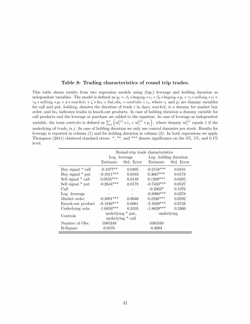
Table 8: Trading characteristics of round trip trades.

This table shows results from two regression models using (log-) leverage and holding duration asindependent variables. The model is defined as yi = β1 ∗ buysigi ∗ ci +β2 ∗ buysigi ∗pi +γ1 ∗ sellsigi ∗ ci +γ2 ∗ sellsigi ∗ pi + η ∗marketi + ζ ∗ koi + δulvolai + controls+ εi, where ci and pi are dummy variablesfor call and put, holdingi denotes the duration of trade i in days, marketi is a dummy for market buyorder, and koi indicates trades in knock-out products. In case of holding duration a dummy variable forcall products and the leverage at purchase are added to the equation. In case of leverage as independent

variable, the term controls is defined as∑

j

(ul

(j)i ∗ ci + ul

(j)i ∗ pi

), where dummy ul

(j)i equals 1 if the

underlying of tradei is j. In case of holding duration we only use control dummies per stock. Results forleverage is reported in column (1) and for holding duration in column (2). In both regressions we applyThompson (2011) clustered standard errors. *, **, and *** denote significance on the 5%, 1%, and 0.1%level.

Round-trip trade characteristicsLog. leverage Log. holding duration

Estimate Std. Error Estimate Std. Error

Buy signal * call -0.1077** 0.0405 -0.2158*** 0.0181Buy signal * put -0.1011*** 0.0163 0.3667*** 0.0178Sell signal * call 0.0525*** 0.0148 0.1269*** 0.0285Sell signal * put -0.2644*** 0.0178 -0.7433*** 0.0527Call - - -0.2063* 0.1076Log. leverage - - -0.8990*** 0.0378Market order -0.2091*** 0.0046 0.2236*** 0.0592Knock-out product -0.1840*** 0.0061 -2.1629*** 0.0748Underlying vola. -1.6850*** 0.3105 -1.8639*** 0.3360

Controlsunderlying * put, underlyingunderlying * call

Number of Obs. 1085349 1085349R-Square 0.9476 0.3093

41

Table 9: Skewness of realized returns.

The table reports robust skewness measures of log-return distributions grouped by TA signal eventsand option type. Panel A reports buy signals and analogues Panel B sell signals. Cloumn 2 and 3show Groeneveld/Meeden skewness measure and Bowley coefficient, respectively. Absolute diff.s betweenthe call bought on buy signal group and the other groups are validated by bootstrapping from theoverall sample (one-sided). 99.9 % confidence internals are reported in parentheses. Column 4 showstwo-sample Kolmogorov-Smirnov test statistics and p-value based on the standardized (by mean andstandard deviation) empirical return distributions of buy signal call (panel A) and sell signal put groupcompared to the particular other groups.

Panel A - Buy Signals

# trades GM skewness Bowley skewness Kolmogorov-SmirnovEstimate Abs. diff. Estimate Abs. diff. KS statistic p-value

Signal, Call 9407 -0.1048 - 0.1993 - - -No Signal, Call 564528 -0.2403 0.1356 -0.0456 0.2449 0.1115 <0.0001

(0.0444) (0.0606)Signal, Put 16286 -0.4482 0.3434 -0.3825 0.5819 0.2080 <0.0001

(0.0470) (0.0648)No Signal, Put 495128 -0.3560 0.2512 -0.2615 0.4608 0.1776 <0.0001

(0.0378) (0.0556)

Panel B - Sell Signals

# trades GM skewness Bowley skewness Kolmogorov-SmirnovEstimate Abs. diff. Estimate Abs. diff. KS statistic p-value

Signal, Put 8498 -0.3035 - -0.1092 - - -No Signal, Put 502916 -0.3628 0.0593 -0.2739 0.1647 0.054128 <0.0001

(0.0391) (0.0575)Signal, Call 22157 -0.2453 0.0582 -0.1666 0.0574 0.056365 <0.0001

(0.0506) (0.0717)No Signal, Call 551778 -0.2374 0.0661 -0.0363 0.0728 0.171503 <0.0001

(0.0478) (0.0652)

42