the role of visual saliency in the automation of seismic ... role of visual saliency in the...

The Role of Visual Saliency in the Automation

of Seismic Interpretation

Muhammad Amir Shafiq *, Tariq Alshawi, Zhiling Long, and Ghassan

AlRegib.

Center for Energy and Geo Processing (CeGP) Georgia Institute of Technology, Atlanta, GA, U.S.A

* Corresponding Author: [email protected]

ABSTRACT

In this paper, we propose a workflow based on SalSi for the detection and delineation of

geological structures such as salt domes. SalSi is a seismic attribute designed based on the

modeling of human visual system that detects the salient features and captures the spatial

correlation within seismic volumes for delineating seismic structures. Using SalSi, we can

not only highlight the neighboring regions of salt domes to assist a seismic interpreter but

also delineate such structures using a region growing method and post-processing. The

proposed delineation workflow detects the salt-dome boundary with very good precision and

accuracy. Experimental results show the e↵ectiveness of the proposed workflow on a real

seismic dataset acquired from the North Sea, F3 block. For the subjective evaluation of

the results of di↵erent salt-dome delineation algorithms, we have used a reference salt-dome

boundary interpreted by a geophysicist. For the objective evaluation of results, we have used

five di↵erent metrics based on pixels, shape, and curvedness to establish the e↵ectiveness of

the proposed workflow. The proposed workflow is not only fast but also yields better results

as compared to other salt-dome delineation algorithms and shows a promising potential in

seismic interpretation.

Keywords— Saliency, SalSi, Seismic attribute, Salt dome delineation, Seismic interpreta-

tion, Data processing, Signal processing.

INTRODUCTION

The evaporation of water from a basin causes the deposition of salt evaporites. Over a long

periods of time, these evaporites, because of their low density, break through sediment layers

often composed of limestone and shale to form diapir-shaped structures called salt domes.

Salt domes may span over several kilometers in the Earth’s subsurface and form stratigraphic

traps for petroleum and gas reservoirs because of their impermeability. Therefore, accurate

localization and delineation of the salt domes in a migrated seismic volume is one of the

key steps in the exploration of oil and petroleum reservoirs. Experienced interpreters can

manually label the boundaries of salt domes by observing and analyzing seismic reflections.

However, with the dramatically increasing size of seismic data, manual labeling is becoming

extremely time consuming and labor intensive. In recent decades, to improve interpretation

e�ciency, researchers have used intelligent computer-aided algorithms to assist the inter-

pretation process. Interpreters beginning with an initial solution can interactively fix the

erroneously detected boundary sections and fine tune the algorithm’s parameters to accu-

rately segment seismic volumes. Therefore, fully- and semi-automated algorithms for seismic

interpretation under the supervision of interpreters have proved their worth both in industry

and academia.

Over the last few decades, researchers have proposed several subsurface structure detection

methods. In particular, there are several works on the detection of salt domes such as edge-

based methods by Zhou et al. (2007); Aqrawi, Boe and Barros (2011); and Amin and Deriche

(2015b), texture-based methods by Berthelot, Solberg and Gelius (2013); Wang et al. (2015);

and Shafiq et al. (2015b), graph-theory-based method by Shi and Malik (2000), active-

contours-based detection by Lewis, Starr and Vigh (2012); Haukas et al. (2013); and Shafiq,

Wang and AlRegib (2015a), machine learning-based methods by Guillen et al. (2015b); Amin

and Deriche (2015a); Guillen et al. (2015a); Larrazabal, Guillen and Gonzalez (2015); and

Amin and Deriche (2016), and di↵erent image processing techniques by Lomask, Biondi and

Shragge (2004); Lomask, Clapp and Biondi (2007); Halpert, Clapp and Biondi (2009); Qi

et al. (2016); Ramirez, Larrazabal and Gonzalez (2016); and Wu (2016). One of the rarely

explored aspect for seismic interpretation is saliency.

Saliency detection attempts to predict areas in images and videos that are interesting to

humans typically called salient regions by relying on low level features that attracts the

human visual system (HVS) (Borji and Itti 2013). As a great deal of research in compu-

tational cognitive science suggest, HVS has evolved to reduce the size of the sensory data

information gathering stage, also known as the task-free visual search, by focusing on the

perceptually salient segments of visual data that convey the most useful information about

the scene (Borji 2015). Features like color contrast, intensity contrast, flicker, and motion

all have been identified as prominent features that help HVS to focus processing resources

on important elements in the surrounding environment. It is commonly believed that HVS

is attracted to localized outliers and novel elements in the environment, which is formulated

as center-surround model by Gao, Mahadevan and Vasconcelos (2008). The center-surround

model compares regions in the visual input to its local surrounding and predicts its saliency.

Several features and detection algorithms for saliency have been proposed in the literature by

Borji and Itti (2013) and Borji (2015). More recently, a 3D FFT-based saliency detection al-

gorithm for videos has been proposed by Long and AlRegib (2015). This algorithm uses a 3D

FFT of a non-overlapping window in the spatial and temporal domains of a video sequence

to compute the spectral energy of the window and compare it with its surrounding regions to

construct the saliency map. The algorithm is e�cient computationally, requires little tuning

of model parameters as compared to other visual saliency algorithms, and provides reliable

results as shown in Long and AlRegib (2015).

In seismic interpretation, visual saliency is important to predict the human interpreters

attention and highlight the areas of interest in seismic sections. Drissi, Chonavel and Boucher

(2008) proposed an algorithm for horizon picking by detecting the salient texture features

in seismic sections by computing entropy at each pixel using two entropy measures: the

Shannon entropy and the generalized cumulative residual entropy. After saliency detection,

Drissi et al. (2008) used active contour for tracking horizons in seismic volume. On the

other hand, Shafiq et al. (2016b) proposed a seismic attribute for salt dome detection based

on visual saliency, SalSi. SalSi highlights the salient areas of a seismic image, i.e. the

neighborhood of salt-dome boundaries, by comparing local spectral features based on 3D

fast Fourier transform (FFT) according to Long and AlRegib (2015). However, to the best

of our knowledge, saliency has not been proposed for salt dome delineation.

In this paper, we propose a workflow based on SalSi for salt dome delineation, which is

a continuation of our previous work (Shafiq et al. 2016a,b), where we proposed SalSi for

seismic interpretation. Using the proposed workflow, we can process seismic volumes in real-

time and perform complex processing procedures more precisely. The rest of the paper is

organized as follows. The proposed workflow for salt dome delineation is presented in section

2. Experimental results on a 3D field data are given in section 3 followed by conclusions in

section 4.

PROPOSED WORKFLOW FOR SALT DOME DELINEATION

The block diagram of the proposed workflow for salt dome delineation is shown in Figure 1.

The migrated 3D seismic data, V, is of size M ⇥ N ⇥K, where M represents the number

of samples of time or depth axis, N represents the number of crosslines, and K represents

the number of inlines. There are four main steps of the proposed workflow as explained in

detail below.

Saliency Detection

We, first, compute saliency using the 3D FFT-based algorithm as proposed in Long and

AlRegib (2015). The 3D FFT-based saliency algorithm obtains saliency maps with ad-

justable resolution, which allows better segmentation of salient objects. The 3D FFT-based

algorithm is computationally inexpensive and requires little tuning of model parameters as

compared to other visual saliency algorithms, which make it advantageous for seismic appli-

cations. The block diagram of 3D FFT-based saliency detection algorithm is also shown in

Figure 1. To obtain the saliency map S, we calculate the 3D FFT spectrum F in a local area

using equation (1), and decompose F into a temporal-change-related component Ft

and a

spatial-change-related component Fs

as

F[µ, ⌫,!] =1

L3

L�1X

m=0

L�1X

n=0

L�1X

k=0

f [m,n, k]e�2⇡i(mµ+n⌫+k!)/L, (1)

Ft

[µ, ⌫,!] = F[µ, ⌫,!]⇥ !pµ2 + ⌫2 + !2

, (2)

Fs

[µ, ⌫,!] = F[µ, ⌫,!]⇥pµ2 + ⌫2p

µ2 + ⌫2 + !2, (3)

where [m,n, k] and [µ, ⌫,!] represent the coordinates in the spatial and frequency domains,

respectively, L defines the size of local data cube, and f [m,n, k] is the seismic image or

section. Subsequently, the spectral energies Et

and Es

are calculated as features based on

absolute mean of temporal- and spatial-change-related components as

Ex

[m,n, k] =1

L3

X

i,j,k

|Fx

|, x 2 (t, s), (4)

where Fx

represents the local spectral volume centered around a voxel [m,n, k]. Applying

the center-surround model, two saliency maps St

and Ss

can be constructed using Et

and

Es

as

Sx

[m,n, k] =1

Q

X

i0,j0,r0

|Ex

[m,n, k]� Ex

[m+ i0, n+ j0, k + r0]|, (5)

where i0, j0, r0 are chosen such that point [m + i0, n + j0, k + r0] is in the immediate

neighborhood of point [m,n, k], such as within a 3⇥ 3⇥ 3 window centered at [m,n, k]. Sx

represents St

or Ss

, Ex

represents Et

or Es

, and Q represents the total number of points

included in the summation in equation 5. The final saliency map S is obtained by averaging

St

and Ss

, and is of same size as of V.

S[m,n, k] = 0.5⇥ St

[m,n, k] + 0.5⇥ Ss

[m,n, k]. (6)

A typical seismic inline section and its normalized saliency map S are shown in Figures 2

and 3, respectively. It can be observed from the Figure 3 that it highlights the boundary of

salt dome, which can be extracted using the following steps of the proposed workflow.

Thresholding

For the application under consideration, the most salient part of a seismic image is the salt-

dome boundary as seen in the saliency map S. The second step of the proposed workflow is

to threshold the saliency map to obtain a binary volume B, which highlights the salt-dome

boundaries.

B[m,n, k] =

8><

>:

1 S[m,n, k] � T

0 Otherwise, (7)

where T represents the threshold. In contrast to the non-salt regions, salt-dome boundaries

have higher S values. Therefore, we assume that the histogram of the volume S follows a

bi-modal distribution. The threshold T can be determined by minimizing the intra-class

variance by optimally dividing all points into two classes. Mathematically, it can be written

as

T = argminT

(�21(T )

T�1X

i=0

p(i) + �22(T )

HX

i=T

p(i)

), (8)

whereH is the number of the quantized gray-levels of S, and p(i), i = 0, · · · , H�1, represents

the probability of points with gray value i. In addition, �21 and �2

2 define the individual class

variances, which can be calculated as follows:

8>>>>><

>>>>>:

�21 =

T�1X

i=0

"i�

T�1X

i=0

ip(i)

p1

#2p(i)

p1, p1 =

T�1X

i=0

p(i)

�22 =

H�1X

i=T

"i�

H�1X

i=T

ip(i)

p2

#2p(i)

p2, p2 =

H�1X

i=T

p(i)

. (9)

Therefore, we can adaptively identify threshold T by exhaustively searching between 0 and

H � 1. Otsu’s method attempts to find a value T by iteratively searching over the possible

probability values such that the interclass variance are maximized. Otsu shows in Otsu (1979)

that the optimum threshold T can be obtained by maximizing the inter-class variance which

is equivalent to minimizing the intra-class variance. Mathematically, it is represented as

T = argmaxT

( T�1X

i=0

p(i)

!(µ1(T )� µ2(T ))

), (10)

where µ1(T ) and µ2(T ) are the mean values of the first and second classes, respectively, at

a threshold T . In the quest of complete automation, Otsu’s method adaptively calculates

the optimum threshold by maximizing the inter-class variance. However, an interpreter can

also interactively fine tune the adaptive threshold to highlight the regions around salt body,

which results in better delineation of salt domes. The output of thresholding is shown in

Figure 4, which highlights the regions around salt-dome boundary i.e. the most salient area

in the saliency map.

Region Growing

Thresholding yields a volume B, same size as that of the 3D seismic volume, V, which

contains noisy and disconnected regions as evident in a seismic inline shown in Figure 4. In

order to extract a salt body from binary volume B, we apply 3D region growing method

as a third step to obtain a closed salt body. In region growing, we randomly select either

one or multiple seed points inside salt dome and keep adding to each seed point a set of

neighboring voxels until they hit the salt boundary. Adams and Bischof (1994) proposed

a robust, rapid, and free-of-parameter-tuning region growing method for the segmentation

of intensity images. In region growing, we select multiple seed points ps1, ps2, ps3, ... psr

and keep adding to each seed point a set of neighboring voxels until a stopping criterion is

met. Voxels that meet a certain criterion form regions R1, R2, R3, ... Rr and are labeled

as allocated voxels. In contrast, voxels in the variant regions that do not meet selected

criteria are labeled as unallocated. We define U as the set of all unallocated voxels in the

neighborhood of labeled regions or salt body, which can be mathematically expressed as

U =

(v

�� v /2r[

i=1

Ri

�� N(v) \r[

i=1

Ri 6= �

), (11)

where a voxel at point [m,n, k] is represented as v for simplification, � represents the empty

set, and N(v) is the neighborhood of voxel v in the 3D volume. In equation (11), we compute

the intersection of neighboring voxels, N(v), and the union of all allocated regions, Ri. If

this intersection is not an empty set, then U contains all the voxels that do not lie inside

allocated regions union. For unlabeled voxels v 2 U , the N(v) falls within just one of the

labeled regions Ri. We define (v) 2 {1, 2, ..., r} as the indexes of neighboring voxels such

that N(v) \ (v) 6= �. In intensity-based region growing, voxels are assigned to particular

regions, Ri, based on their intensity values, I(v). �(v) define the intensity di↵erence at voxel

v and its adjacent labeled region Ri as

�(v) = |I(v)�meann2Ri(I(n))|, (12)

where I(v) defines the intensity values at the voxels v. If N(v) is close to more than one Ri,

then (v) takes the value of v such that �(v) at Ri is minimized.

(v) = minv2U

{�(v)}. (13)

In region growing, we select an initial seed point, ps, randomly inside the salt body and it

continues to grow into a region until it hits the highlighted boundary (labeled as ones in

B). The seeded region growing continues until all the voxels are allocated to region Ri. This

process can be mathematically expressed as follows:

SD =

8<

:[

pg2B

R|N(pg) 6= 1

9=

; , (14)

where N(pg) is the neighboring region of the area starting from the seed point ps and SD is

the salt-dome body detected after region growing. In the nutshell, we apply region growing on

the binarized volume, B, obtained by thresholding saliency map, S, to yield a salt-dome body,

SD, with a seed point selected randomly inside salt body. If we want to segment multiple

disconnected salt bodies then we can select multiple seed points that will independently grow

into salt dome. Our dataset (details are given in experimental results section) has only one

salt dome and we have randomly selected only one seed point for whole volume to initiate

3D region growing. The output of 3D region growing with an initial seed point highlighted

in red is shown in Figure 5.

Seed Point Selection

The seed point, ps, for region growing can be selected either automatically by computer algo-

rithms or manually by the seismic interpreter. The automatic seed point selection methods

for 2D and 3D data, based on directionality and tensor decomposition, are given in Wang

et al. (2015) and Shafiq et al. (2017), respectively. However, automatic seed point selection

methods are computationally expensive and may fail in the presence of noise and chaotic

horizons. Automatic seed point selection methods under such circumstances may result in

the considerable loss of time and computation e↵ort. In manual seed point selection, the

seismic interpreter can interactively choose any arbitrarily random point inside volume as

long as it is inside salt body. The interpreter can also choose multiple seed points to speed

up the region growing. The time required by geophysicist interpreter to manually select ps

is insignificant as compared to automatic ps selection. Therefore, in this paper, we have

manually selected a seed point inside salt body.

Post-Processing

To bridge the gaps between the output of region growing and the salt-dome boundary,

we apply morphological operations, which includes dilation and perimeter extraction. By

expanding the detected salt body, the dilation operation matches the detected salt-dome

boundary with the reference as closely as possible and alleviate the e↵ects of window sizes

in the calculation of the saliency. The dilated salt body is mathematically given as

SDD = SD �HD, (15)

where � represents dilation and HD represents the structural element of dilation (Gonza-

lez and Woods 2008). The final step of the proposed workflow is to detect boundary by

extracting the perimeter of the salt body, which can be mathematically expressed as

SDB = {v 2 SDD|N26[v]� SDD 6= �} , (16)

where SDB is the detected salt-dome boundary and N26[v] defines the 26 neighboring voxels

of v in a 3D space. The dilated salt-dome and the output of post-processing are shown in

Figures 6 and 7, respectively.

EXPERIMENTAL RESULTS

In this section, we demonstrate the e↵ectiveness of the proposed workflow for salt dome

delineation. We have used the real seismic dataset acquired from the Netherlands o↵shore,

F3 block in the North Sea whose size is 24 x 16 km2 (dGB Earth Sciences B.V. 1987).

The seismic volume that contains the salt-dome structure has an inline number ranging

from 151 to 501, a crossline number ranging from 701 to 981, and a time direction starting

from 1, 300ms sampled every 4ms. The bin size across the inline and crossline directions

is 25 meters. In this paper, we use a non-overlapping cube of size 3 ⇥ 3 ⇥ 3 for saliency

calculation. The size of structuring element in the post-processing operations is equal to

the side length of the cube i.e. 3. The output of the proposed workflow and the results of

di↵erent algorithms for salt dome delineation on seismic inline sections 360, 372, 390, and

408 are shown in Figure 8, with the reference boundary manually labeled by a geophysicist

in green. The cyan, blue, yellow, magenta, black, and red lines represent the boundaries

detected by Wang et al. (2015), Shafiq et al. (2015b), Berthelot et al. (2013), Aqrawi et al.

(2011), Amin and Deriche (2016), and the proposed workflow, respectively.

The output of di↵erent state-of-the-art algorithms have significant di↵erences from the ref-

erence boundary as observed in the Figure 8. The output of the texture-based method by

Berthelot et al. (2013) and learning-based method by Amin and Deriche (2016) extends

beyond the salt-dome boundary as seen in the bottom left corner of Figure 8a-b. The edge-

based method by Aqrawi et al. (2011) deviates from the reference in the absence of strong

seismic reflections as observed in the bottom right section of salt dome in Figure 8c. Fur-

thermore, edge-based method by Aqrawi et al. (2011) and texture-based method by Wang

et al. (2015) detects only the right side of salt dome and is not able to detect the associated

event on the left side as observed in Figure 8a-b. The output of texture-based methods

presented in Wang et al. (2015) and Shafiq et al. (2015b) degrades in the absence of strong

texture as seen in Figure 8c. The proposed method captures the salient areas in the volume

and attempt to highlight the variations of salt dome across seismic volume. However, this

method yields less accurate results in the areas where the variations in salt-dome boundary

are comparatively less as compared to their neighboring seismic inlines. As shown in Fig-

ure 8a-c, the proposed method diverges from the reference boundary in the bottom left areas

of salt dome. Subjectively, it can be argued that the boundaries detected by all aforemen-

tioned algorithms lie close to the reference boundary. However, due to tortuous salt-dome

boundaries, it is di�cult to deduce which method outperforms other methods in terms of

its delineation precision and accuracy. Therefore, we have used five di↵erent metrics to

objectively evaluate the results of di↵erent salt-dome delineation algorithms.

To investigate the results of delineation algorithms per pixel, we have used accuracy, preci-

sion, and F-score (Powers 2011), which are usually used as an objective evaluation metrics

in binary classification. True positives (TP) and true negatives (TN) measures, at each

seismic inline, the number of pixels that belong to the salt-dome and are correctly identified

as such and vice versa. On the other hand, false positives (FP) and false negatives (FN)

measures, at each seismic inline, the number of non-salt pixels classified as salt pixels and

salt pixels classified as non-salt pixels, respectively. Accuracy, precision, and F-score are

then calculated using

Accuracy =TP + TN

TP + FN + FP + TN, (17)

Precision =TP

TP + FP, (18)

Recall =TP

TP + FN, (19)

F-score = 2 · Precision ·Recall

Precision+Recall. (20)

The accuracy and precision of various delineation algorithms for fifty seven consecutive

seismic inlines are shown in Figures 9a and 9b, respectively. The accuracy and precision

values of the proposed method are closer to one that not only support that it is more

accurate but also more precise in delineating salt-domes within seismic inlines. F-score,

which measures the test accuracy, is the harmonic mean of precision and recall. F-scores

of various delineation algorithms for fifty seven consecutive seismic inlines are shown in

Figure 9c, which demonstrates that the proposed workflow, on most inlines, surpass other

methods of salt dome delineation. The mean and standard deviation (S.D) of accuracy,

precision, and F-scores of various salt-dome delineation algorithms for the plots shown in

Figure 9 are presented in Table 1, with the best scores highlighted in boldface. It can be

observed that the proposed workflow outperforms other salt-dome delineation algorithms in

terms of mean and standard deviation, except the standard deviation of F-score, which is

slightly less than the texture-based method by Shafiq et al. (2015b).

Accuracy, precision, and F-scores provided the statistical evaluation of results in terms of

pixels. To evaluate the results of di↵erent salt-dome delineation algorithms based on their

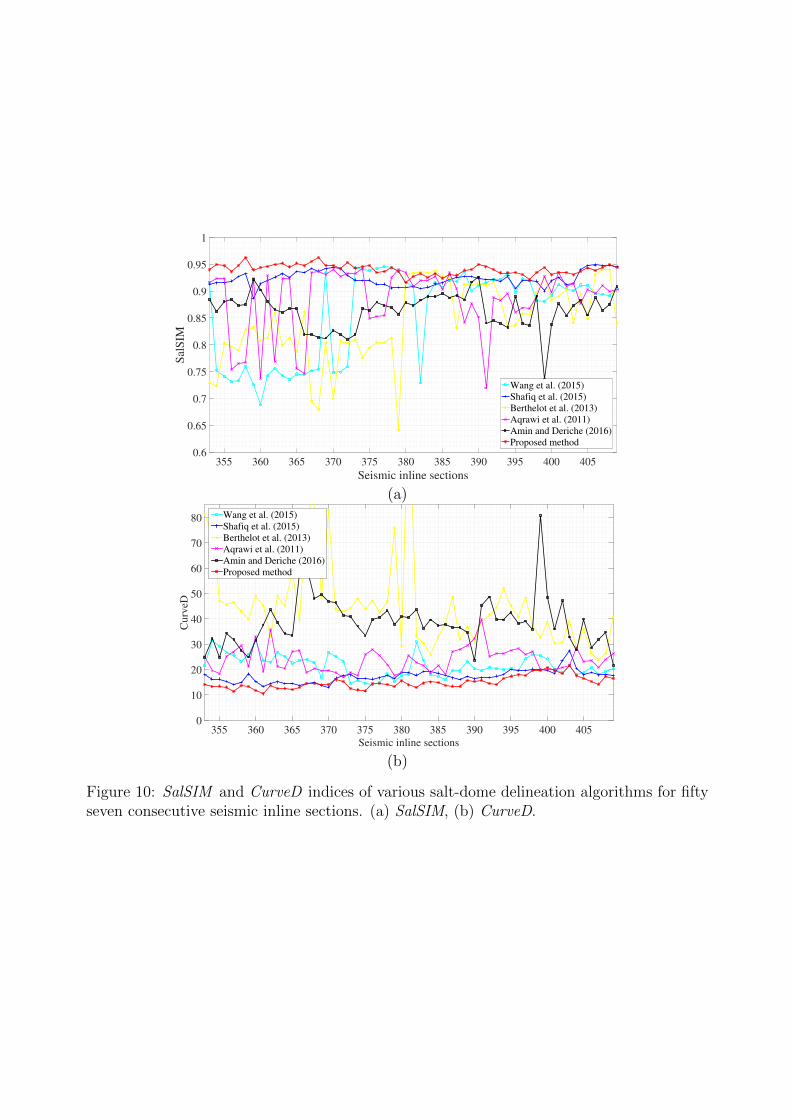
shape and curvature, we have used two di↵erent evaluation metrics. First, SalSIM, pro-

posed by Wang et al. (2015), measures the similarity between the reference and the detected

salt-dome boundary using the Frechet distance-based similarity index. The SalSIM index

ranges between 0 to 1, with a higher value indicating a greater similarity between the two

boundaries under comparison. Second, CurveD, proposed by Shafiq et al. (2017), computes

the distance between the reference and the detected salt-dome boundary based on their

shape and curvedness. If two curves are similar in shape and curvature then the CurveD

index is closer to zero and vice versa. The SalSIM and CurveD indices of various salt-dome

delineation algorithms for fifty seven consecutive seismic inlines are shown in Figures 10a

and 10b, respectively. Furthermore, the mean and standard deviation (S.D.) of SalSIM and

CurveD indices, illustrated in Figure 10, are given in Table 2, with the best scores highlighted

in boldface. Figure 10 and Table 2 illustrate that the best results are obtained using the

proposed method, which outperforms the state-of-the-art methods for salt dome delineation.

We also calculate the time required by each algorithm for delineation and results are summa-

rized in Table 2. It can be observed that the proposed workflow is not only computationally

very e�cient but also the fastest among all aforementioned algorithms. Finally, the detected

3D salt body is displayed in Figure 11, which illustrates that the proposed method not only

outlines the major structure of the salt body but also highlight the details of local structures

e↵ectively to show the formation of salt dome. Experimental results presented in this sec-

tion show that the proposed workflow can be a useful addition to the interpreters toolbox

for delineating important geological structures.

CONCLUSION

A seismic attribute based on visual saliency, SalSi, has many applications in seismic inter-

pretation such as salt dome delineation, tracking salt domes in a seismic volume, algorithms

initialization, reducing time computation, seismic retrieval, and labeling, etc. In this paper,

we proposed a workflow based on SalSi for salt dome delineation within migrated seismic

volumes. The experimental results on a real seismic dataset from the North Sea, F3 block

show the e↵ectiveness of the proposed workflow. The subjective and objective evaluation of

the results show that the proposed workflow is very fast and outperforms the state-of-the-art

algorithms for salt dome delineation. The results presented in this paper show a promising

future of the proposed workflow for salt dome delineation and excellent potential in seismic

interpretation that can not only automate but can e↵ectively reduce the time as well. This

workflow can also be easily modified to highlight chaotic horizons and faults within seismic

volumes, which requires further investigation.

ACKNOWLEDGMENTS

This work is supported by the Center for Energy and Geo Processing (CeGP) at the Georgia

Tech and KFUPM. We would like to thank dGB Earth Sciences for making the F3 seismic

data available publicly.

REFERENCES

Adams R. and Bischof L. 1994. Seeded region growing. IEEE Transactions on Pattern

Analysis And Machine Intelligence 16, 641–647.

Amin A. and Deriche M. 2015a. A hybrid approach for salt dome detection in 2D and 3D

seismic data. IEEE International Conference on Image Processing (ICIP), 1–5.

——– 2015b. A new approach for salt dome detection using a 3D multidirectional edge

detector. Applied Geophysics 12, 334–342.

——– 2016. Salt-dome detection using a codebook-based learning model. IEEE Geoscience

and Remote Sensing Letters 13, 1636–1640.

Aqrawi A. A., Boe T. H. and Barros S. 2011. Detecting salt domes using a dip guided

3D Sobel seismic attribute. 81st SEG Annual Meeting, San Antonio, Texas, Expanded

Abstracts, 1014–1018.

Berthelot A., Solberg A. H. and Gelius L. J. 2013. Texture attributes for detection of salt.

Journal of Applied Geophysics 88, 52–69.

Borji A. 2015. What is a salient object? A dataset and a baseline model for salient object

detection. IEEE Transactions on Image Processing 24, 742–756.

Borji A. and Itti L. 2013. State-of-the-art in visual attention modeling. IEEE Transactions

on Pattern Analysis and Machine Intelligence 35, 185–207.

dGB Earth Sciences B.V. 1987. The Netherlands

O↵shore, The North Sea, F3 Block - Complete.

https://opendtect.org/osr/pmwiki.php/Main/Netherlands/O↵shoreF3BlockComplete4GB.

Drissi N., Chonavel T. and Boucher J. 2008. Salient features in seismic images. OCEANS

2008 - MTS/IEEE Kobe Techno-Ocean, 1–4.

Gao D., Mahadevan V. and Vasconcelos N. 2008. On the plausibility of the discriminant

center-surround hypothesis for visual saliency. Journal of Vision 8, 1–18.

Gonzalez R. and Woods R. 2008. Digital image processing. Pearson/Prentice Hall,

ISBN:9780131687288.

Guillen P., Larrazabal G., Gonzalez G., Boumber D. and Vilalta R. 2015a. Supervised learn-

ing to detect salt body. 85th SEG Annual Meeting, New Orleans, Louisiana, Expanded


Guillen P., Larrazabal G., Gonzalez G. and Sineva D. 2015b. Detecting salt body using

texture classification. 14th International Congress of the Brazilian Geophysical Society &

EXPOGEF, Rio de Janeiro, Brazil, Expanded Abstracts, 3-6 August, 1155–1159.

Halpert A. D., Clapp R. G. and Biondi B. 2009. Seismic image segmentation with multiple

attributes. 79th SEG Annual Meeting, Houston, Texas, Expanded Abstracts, 3700–3704.

Haukas J., Ravndal O. R., Fotland B. H., Bounaim A. and Sonneland L. 2013. Automated

salt body extraction from seismic data using level set method. First Break 31, (4), 35–42.

Larrazabal G., Guillen P. and Gonzalez G. 2015. A novel salt body detection workflow. 77th

EAGE Conference and Exhibition, Madrid, Spain, Expanded Abstracts, Tu G107 05.

Lewis W., Starr B. and Vigh D. 2012. A level set approach to salt geometry inversion in full-

waveform inversion. 82nd SEG Annual Meeting, Las Vegas, Nevada, Expanded Abstracts,

1–5.

Lomask J., Biondi B. and Shragge J. 2004. Image segmentation for tracking salt boundaries.

74th SEG Annual Meeting, Houston, Texas, Expanded Abstracts, 2443–2446.

Lomask J., Clapp R. G. and Biondi B. 2007. Application of image segmentation to tracking

3D salt boundaries. Geophysics 72, (4), P47–P56.

Long Z. and AlRegib G. 2015. Saliency detection for videos using 3D FFT local spectra.

Proceedings of SPIE 9394, 93941G–6.

Otsu N. 1979. A threshold selection method from gray-level histograms. IEEE Transactions

on Systems, Man and Cybernetics 9, 62–66.

Powers D. M. W. 2011. Evaluation: From Precision, Recall and F-Measure to ROC, In-

formedness, Markedness & Correlation. Journal of Machine Learning Technologies 2, (1),

37–63.

Qi J., Lin T., Zhao T., Li F. and Marfurt K. 2016. Semisupervised multiattribute seismic

facies analysis. Interpretation 4, (1), SB91–SB106.

Ramirez C., Larrazabal G. and Gonzalez G. 2016. Salt body detection from seismic data via

sparse representation. Geophysical Prospecting 64, 335–347.

Shafiq M., Wang Z., AlRegib G., Amin A. and Deriche M. 2017. A texture-based interpreta-

tion workflow with application to delineating salt domes. Interpretation 5, (3), SJ1–SJ19.

Shafiq M. A., Alshawi T., Long Z. and AlRegib G. 2016a. The role of visual saliency in

seismic interpretation with an application to salt dome delineation. SIAM conference on

Imaging Science, New Mexico, USA, May 23-26.

——– 2016b. SalSi: A new seismic attribute for salt dome detection. IEEE International

Conference on Acoustics, Speech and Signal Processing (ICASSP), Shanghai, China, 20-25

March, 1876–1880.

Shafiq M. A., Wang Z. and AlRegib G. 2015a. Seismic interpretation of migrated data using

edge-based geodesic active contours. IEEE Global Conference on Signal and Information

Processing (GlobalSIP), Orlando, Florida, Dec. 14-16.

Shafiq M. A., Wang Z., Amin A., Hegazy T., Deriche M. and AlRegib G. 2015b. Detection

of salt-dome boundary surfaces in migrated seismic volumes using gradient of textures.

85th SEG Annual Meeting, New Orleans, Louisiana, Expanded Abstracts, 1811–1815.

Shi J. and Malik J. 2000. Normalized cuts and image segmentation. IEEE Transactions on

Pattern Analysis and Machine Intelligence 22, 888–905.

Wang Z., Hegazy T., Long Z. and AlRegib G. 2015. Noise-robust detection and tracking

of salt domes in postmigrated volumes using texture, tensors, and subspace learning.

Geophysics 80, (6), WD101–WD116.

Wu X. 2016. Methods to compute salt likelihoods and extract salt boundaries from 3D

seismic images. Geophysics 81, (6), IM119–IM126.

Zhou J., Zhang Y., Chen Z. and Li J. 2007. Detecting boundary of salt dome in seismic data

with edge detection technique. 85th SEG Annual Meeting, San Antonio, Texas, Expanded


LIST OF FIGURES

1 The block diagram of the proposed workflow.

2 A typical seismic inline containing salt dome.

3 The saliency map of a seismic inline.

4 The binary map of a seismic inline.

5 The output of 3D region growing with a seed point highlighted in red.

6 Dilated salt dome.

7 The green line depicts the output of post-processing.

8 The experimental results of salt dome delineation on di↵erent seismic inline sec-

tions. Green: Reference boundary manually interpreted by a geophysicist, Cyan: Wang

et al. (2015), Blue: Shafiq et al. (2015b), Yellow: Berthelot et al. (2013), Magenta: Aqrawi

et al. (2011), Black: Amin and Deriche (2016), Red: Proposed Workflow. (a) Seismic inline

section 360, (b) Seismic inline section 372, (c) Seismic inline section 390, (d) Seismic inline

section 408.

9 Accuracy, precision, and F-scores of various salt-dome delineation algorithms for

fifty seven consecutive seismic inline sections. (a) Accuracy, (b) Precision, (c) F-score.

10 SalSIM and CurveD indices of various salt-dome delineation algorithms for fifty

seven consecutive seismic inline sections. (a) SalSIM, (b) CurveD.

11 The detected 3D salt body.

LIST OF TABLES

1 Mean and standard deviation of accuracy, precision, and F-scores for various salt-

dome delineation algorithms.

2 Mean and standard deviation of SalSIM and CurveD indices, and time required by

various salt-dome delineation algorithms.

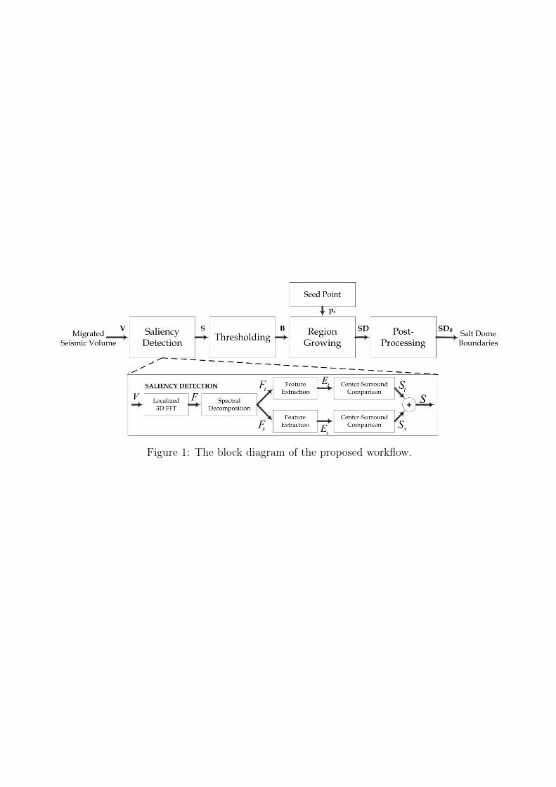
Figure 1: The block diagram of the proposed workflow.

Figure 2: A typical seismic inline containing salt dome.

Crosslines749 799 849 899 949

Tim

e (m

s)

1380

1460

1540

1620

1700

0.1

0.2

0.3

0.4

0.5

0.6

Figure 3: The saliency map of a seismic inline.

Figure 4: The binary map of a seismic inline.

Figure 5: The output of 3D region growing with a seed point highlighted in red.

Figure 6: Dilated salt dome.

Figure 7: The green line depicts the output of post-processing.

(a)

(b)

(c)

(d)

Figure 8: The experimental results of salt dome delineation on di↵erent seismic inline sec-tions. Green: Reference boundary manually interpreted by a geophysicist, Cyan: Wang et al.(2015), Blue: Shafiq et al. (2015b), Yellow: Berthelot et al. (2013), Magenta: Aqrawi et al.(2011), Black: Amin and Deriche (2016), Red: Proposed Workflow. (a) Seismic inline section360, (b) Seismic inline section 372, (c) Seismic inline section 390, (d) Seismic inline section408.

Seismic inline sections355 360 365 370 375 380 385 390 395 400 405

Acc

ura

cy

0.85

0.9

0.95

1

Wang et al. (2015)Shafiq et al. (2015)Berthelot et al. (2013)Aqrawi et al. (2011)Amin and Deriche (2016)Proposed method

(a)


Pre

cisi

on

0.75

0.8

0.85

0.9

0.95

1


(b)


F-s

core

0.85

0.9

0.95

1


(c)

Figure 9: Accuracy, precision, and F-scores of various salt-dome delineation algorithms forfifty seven consecutive seismic inline sections. (a) Accuracy, (b) Precision, (c) F-score.

355 360 365 370 375 380 385 390 395 400 405

Seismic inline sections

0.6

0.65

0.7

0.75

0.8

0.85

0.9

0.95

1

Sal

SIM


(a)


Curv

eD

0

10

20

30

40

50

60

70

80 Wang et al. (2015)Shafiq et al. (2015)Berthelot et al. (2013)Aqrawi et al. (2011)Amin and Deriche (2016)Proposed method

(b)

Figure 10: SalSIM and CurveD indices of various salt-dome delineation algorithms for fiftyseven consecutive seismic inline sections. (a) SalSIM, (b) CurveD.

Figure 11: The detected 3D salt body.

Table 1: Mean and standard deviation of accuracy, precision, and F-scores for various salt-dome delineation algorithms.

MethodsAccuracy (%) Precision (%) F-scoreMean S.D. Mean S.D. Mean S.D.

Wang et al. (2015) 96.32 1.30 96.40 1.85 0.9403 0.0232Shafiq et al. (2015b) 97.35 0.50 94.86 2.59 0.9591 0.0070Berthelot et al. (2013) 95.84 4.75 96.26 1.77 0.9239 0.1085Aqrawi et al. (2011) 95.72 1.22 89.79 3.20 0.9361 0.0176Amin and Deriche (2016) 96.69 2.23 95.26 3.24 0.9470 0.0447Proposed Workflow 97.59 0.45 97.76 1.19 0.9616 0.0072

Table 2: Mean and standard deviation of SalSIM and CurveD indices, and time required byvarious salt-dome delineation algorithms.

MethodsSalSIM CurveD

Time(s)Mean S.D. Mean S.D.

Wang et al. (2015) 0.8573 0.0844 21.5004 4.2859 11.4895Shafiq et al. (2015b) 0.9232 0.0136 17.3355 2.4872 63.3162Berthelot et al. (2013) 0.8439 0.0730 45.9306 19.7698 33.5447Aqrawi et al. (2011) 0.8845 0.0605 23.8682 4.8281 0.98110Amin and Deriche (2016) 0.8643 0.0333 38.7502 9.6533 0.68480Proposed Workflow 0.9405 0.0095 14.8835 2.4268 0.39520

the role of visual saliency in the automation of seismic ... role of visual saliency in the...

Documents