the same bond at different prices: identifying search ...feldhutter.com/search.pdf · the same bond...
TRANSCRIPT

The Same Bond at Different Prices:Identifying Search Frictions andSelling Pressures
Peter FeldhutterLondon Business School
I propose a new measure that identifies when the market price of an over-the-counter tradedasset is below its fundamental value due to selling pressure. The measure is the differencebetween prices paid by small traders and those paid by large traders. In a model for over-the-counter trading with search frictions and periods with selling pressures, I show that thismeasure identifies liquidity crises (i.e., high number of forced sellers). Using a structuralestimation, the model is able to identify liquidity crises in the U.S. corporate bond marketbased on the relative prices paid by small and large traders. New light is shed on two crises,the downgrade of General Motors and Ford in 2005 and the subprime crisis (JELD4, D83,G01, G12).
1. Introduction
We know that asset prices can temporarily decrease below their fundamentalvalue when there is selling pressure—i.e., when many investors seek to sellthe asset at the same time.Duffie (2010) reviews recent evidence in his2010 Presidential Address to the American Finance Association. Identifyingwhen this occurs is difficult. This is because the event that causes sellingpressure typically reveals new information about the fundamental value of theasset. Disentangling selling pressure effects from information effects is at bestchallenging.
The main contribution of this article is to propose a measure that identifieswhen there is selling pressure in over-the-counter markets. Selling pressure is
I am very grateful to David Lando and Lasse Heje Pedersen for many helpful comments and discussions andto Jens Dick-Nielsen for discussions regarding the TRACE database. I thank Viral Acharya, Darrell Duffie,Rene Garcia, Soren Hvidkjær, Jesper Rangvid, Norman Schurhoff, Carsten Sorensen, and seminar participantsat the Second International Financial Research Forum in Paris, Second Erasmus Liquidity Conference inRotterdam, 2009 MTS Conference on Financial Markets in London, Doctoral Course at the University ofLausanne, 2009 European Finance Association meeting in Bergen, Nykredit Symposium 2009, D-Caf meetingin Helsingor 2010, Danish Central Bank, Aarhus School of Business, University of Copenhagen, CopenhagenBusiness School, London Business School, New York Fed, University of Toronto, HEC Paris, Boston College,University of Chicago, Rochester, Boston University, University of Lausanne, Goethe-Universitat Frankfurt,Manchester Business School, and University of Cologne for useful suggestions. I thank the Danish SocialScience Research Council for financial support. I also thank the editor, Matthew Spiegel, and an anonymousreferee for many valuable suggestions. Send correspondence to Peter Feldhutter, London Business School,Regent’s Park, London NW1 4SA, United Kingdom; telephone: +44 (0) 20 7000 8277; fax: +44 (0)20 70007001. E-mail:[email protected].
c© The Author 2011. Published by Oxford University Press on behalf of The Society for Financial Studies.All rights reserved. For Permissions, please e-mail: [email protected]:10.1093/rfs/hhr093 Advance Access publication October 7, 2011
by guest on March 20, 2012
http://rfs.oxfordjournals.org/D
ownloaded from

TheReview of Financial Studies / v 25 n 4 2012
definedas times when the number of sellers relative to the number of buyers isunusually high. In over-the-counter markets, an asset simultaneously trades atdifferent prices because prices are negotiated bilaterally. The price differencebetween small trades and large trades at a given point in time identifies sellingpressure. If large traders trade at unusually low prices relative to small traders,there is selling pressure.
In contrast to the existing literature, the measure does not rely on realizedreturns. There are two approaches in the current literature. One approachis to look at asset returns around an event that is unlikely to contain newinformation about asset value. If cumulative returns are negative around theevent and rebound fully or partially during a period after, there has been sellingpressure. Examples of this approach includeCoval and Stafford(2007) andChen, Noronha, and Singhal(2004). This approach is limited to information-free events. Another approach is to control for new information and see ifabnormal returns are negative around the event and subsequently rebound.Mitchell, Pedersen, and Pulvino(2007) andNewman and Rierson(2004)take this approach. If the event reveals new information about fundamentalasset value, it can be challenging to adjust abnormal returns correctly. Forexample,Ellul, Jotikasthira, and Lundblad(2011) andAmbrose, Cai, andHelwege(2009) both study selling pressure in U.S. corporate bonds arounddowngrades. They use similar datasets and reach conflicting conclusionsregarding the importance of selling pressure. Clearly a downgrade containsinformation about firm quality, and it is difficult to control for the impactof this information. In this article, selling pressure is identified throughdifferences in prices occurring simultaneously. Changes in fundamental valueare automatically controlled for since the information effect is the same forboth small and large trades. Furthermore, selling pressure can be identified in“real-time.” Previous approaches identify selling pressure ex post through thesubsequent reversal of returns after an event.
In a theoretical model, I find support for the small trade minus large trademeasure as an identifier of selling pressure. My model is a variant of thesearch model inDuffie, Garleanu, and Pedersen(2005). Empirically, I studythe corporate bond market, so the model is adapted to the structure of thismarket. There is a corporate bond traded in the model. Investors switchrandomly between needing liquidity or not. Investors trade through a dealerwhom they find at random with different search intensities. A high searchintensity implies that the investor finds a counterparty fast. I interpret such aninvestor as a sophisticated/large one. An investor with a low search intensityis interpreted as an unsophisticated/small investor. Once an investor meetsa dealer, they bargain, and the resulting price reflects their alternatives toimmediate trade. One alternative is to cut off negotiations and search for a newcounterparty. This alternative is particularly strong for large investors who findcounterparties fast. Therefore, large investors negotiate tighter bid-ask spreads.The alternative of searching for a new counterparty is also strong for buyers in
1156
by guest on March 20, 2012
http://rfs.oxfordjournals.org/D
ownloaded from

TheSame Bond at Different Prices: Identifying Search Frictions and Selling Pressures
a market in which there is selling pressure. This is because there are currentlymany sellers. The combined advantages of being a large buyer and a buyerin a market experiencing selling pressure lead to significant price discounts.These price discounts are larger than for a small buyer in a market with sellingpressure, because the “threat” of looking for another seller is less forceful fora small buyer.
In equity markets, it is well known that block trades sell at a discount.This is documented byKraus and Stoll(1972) and supported by information-based models such asKyle’s (1985) model. The predictions in my search-basedmodel are different from predictions in information-based models. In a marketwhere the numbers of sellers and buyers are balanced, large traders in a search-based model transact at better prices. The reason is that they negotiate tighterbid-ask spreads due to their stronger outside options. In information-basedmodels, large traders sell at lower prices than small traders. This is becausethey are likely to have private information about asset value. In addition,asset price dynamics under selling pressure are different in the two models. Ininformation-based models, a block trade occurs at a discount and subsequentsmall trades also occur at (slightly smaller) discounts. In the search modelhere, the pattern is different: At times when there is selling pressure, smalltraders trade at high prices and large traders trade at low prices; the timeordering of trades does not matter. This is because, compared with smallbuyers, large buyers can more quickly “shop around” among numerous sellers.As a consequence, they negotiate larger price discounts.
Another contribution to the literature is that I propose and carry out amaximum likelihood approach to estimate parameters of the model. I usetransaction data from the TRACE database for the period from October 2004to June 2009. The TRACE database contains practically all corporate bondtransactions even though trading occurs over the counter. There is a growingliterature on search models, but to my knowledge no one has structurallyestimated a model before. The estimation approach allows me to empiricallyidentify periods of selling pressure.
A third contribution to the literature is that I shed new light on recent selling-pressure episodes in the U.S. corporate bond market. There are two majorincidents of selling pressure according to the empirical results. In May 2005,S&P downgraded General Motors (GM) and Ford to speculative grade, causingstrong selling pressure in their bonds. In the preceding months, selling pressureintensified as a downgrade became more likely, consistent with findings inAcharya, Schaefer, and Zhang(2008). My results show that selling pressurewas largely isolated to GM and Ford bonds. The time pattern of selling pressurein GM bonds was different from that in Ford bonds. Selling pressure in GMbonds peaked in May because GM was downgraded by both S&P and Fitchand dropped out of the important Lehman investment-grade index. In contrast,selling pressure in Ford bonds decreased in May because Ford was downgradedonly by S&P and remained in the Lehman index. The second period with
1157
by guest on March 20, 2012
http://rfs.oxfordjournals.org/D
ownloaded from
The Review of Financial Studies / v 25 n 4 2012
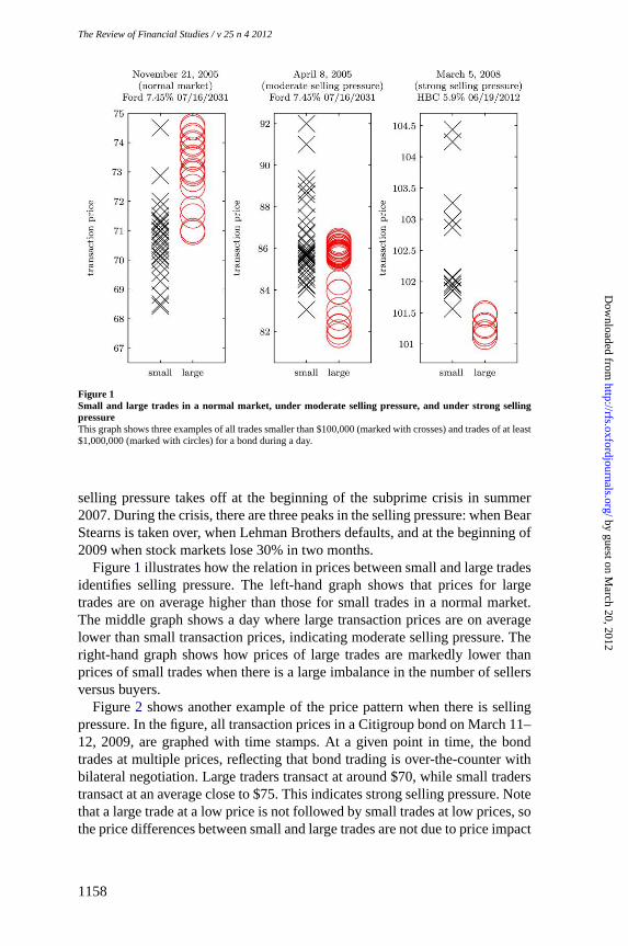
Figure 1Small and large trades in a normal market, under moderate selling pressure, and under strong sellingpressureThis graph shows three examples of all trades smaller than$100,000 (marked with crosses) and trades of at least$1,000,000 (marked with circles) for a bond during a day.
selling pressure takes off at the beginning of the subprime crisis in summer2007. During the crisis, there are three peaks in the selling pressure: when BearStearns is taken over, when Lehman Brothers defaults, and at the beginning of2009 when stock markets lose 30% in two months.
Figure1 illustrates how the relation in prices between small and large tradesidentifies selling pressure. The left-hand graph shows that prices for largetrades are on average higher than those for small trades in a normal market.The middle graph shows a day where large transaction prices are on averagelower than small transaction prices, indicating moderate selling pressure. Theright-hand graph shows how prices of large trades are markedly lower thanprices of small trades when there is a large imbalance in the number of sellersversus buyers.
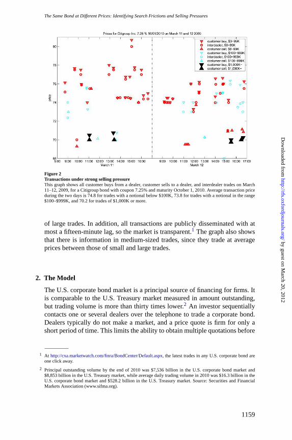
Figure2 shows another example of the price pattern when there is sellingpressure. In the figure, all transaction prices in a Citigroup bond on March 11–12, 2009, are graphed with time stamps. At a given point in time, the bondtrades at multiple prices, reflecting that bond trading is over-the-counter withbilateral negotiation. Large traders transact at around $70, while small traderstransact at an average close to $75. This indicates strong selling pressure. Notethat a large trade at a low price is not followed by small trades at low prices, sothe price differences between small and large trades are not due to price impact
1158
by guest on March 20, 2012
http://rfs.oxfordjournals.org/D
ownloaded from
The Same Bond at Different Prices: Identifying Search Frictions and Selling Pressures
Figure 2Transactions under strong selling pressureThis graph shows all customer buys from a dealer, customer sells to a dealer, and interdealer trades on March11–12, 2009, for a Citigroup bond with coupon 7.25% and maturity October 1, 2010. Average transaction priceduring the two days is 74.8 for trades with a notional below$100K, 73.8 for trades with a notional in the range$100–$999K, and 70.2 for trades of$1,000K or more.
of large trades. In addition, all transactions are publicly disseminated with atmost a fifteen-minute lag, so the market is transparent.1 The graph also showsthat there is information in medium-sized trades, since they trade at averageprices between those of small and large trades.
2. The Model
The U.S. corporate bond market is a principal source of financing for firms. Itis comparable to the U.S. Treasury market measured in amount outstanding,but trading volume is more than thirty times lower.2 An investor sequentiallycontacts one or several dealers over the telephone to trade a corporate bond.Dealers typically do not make a market, and a price quote is firm for only ashort period of time. This limits the ability to obtain multiple quotations before
1 At http://cxa.marketwatch.com/finra/BondCenter/Default.aspx, the latest trades in any U.S. corporate bond areone click away.
2 Principal outstanding volume by the end of 2010 was$7,536 billion in the U.S. corporate bond market and$8,853 billion in the U.S. Treasury market, while average daily trading volume in 2010 was$16.3 billion in theU.S. corporate bond market and$528.2 billion in the U.S. Treasury market. Source: Securities and FinancialMarkets Association (www.sifma.org).
1159
by guest on March 20, 2012
http://rfs.oxfordjournals.org/D
ownloaded from

TheReview of Financial Studies / v 25 n 4 2012
committing to a trade.3 Hence,prices are outcomes of a bargaining game,determined in part by the ease with which investors find counterparties andthe relative number of investors currently looking to buy or sell. The followingmodel captures these important features of the market.
The economy is populated by two kinds of agents, investors and dealers,who are risk-neutral and infinitely lived. They consume a nonstorable con-sumption good used as numeraire, and their time preferences are given by thediscount rater > 0. Time is continuous, starts att = 0, and goes on forever.
Investors have access to a risk-free bank account paying interest rater . Thebank account can be viewed as a liquid security that can be traded instantly. Torule out Ponzi schemes, the valueWt of an investor’s bank account is boundedfrom below. In addition, investors have access to an over-the-counter corporatebond market for a credit-risky bond. There is a continuum of credit-risky firmsthat issue these bonds. If a firm defaults, it is replaced by an identical newfirm. The bond pays coupons at the constant rate of C units of consumptionper year. The bond has expected maturityT and face valueF , meaning thatit matures randomly according to a Poisson process with intensityλT = 1/TandpaysF at maturity. The bond defaults with intensityλD andpays a fraction(1− f )F of face value in default. The total amount outstanding of the bond attime 0 isA where 0< A < 1. When bonds mature or default, firms issue newbonds to replace them, so the total issue intensity is(λD + λT )A. This impliesthat the amount outstanding of bonds at any point in time isA. When bondsare issued, they are sold through the dealers. I do not model the interactionbetween dealers and firms, so the issued bonds appear as extra bonds dealerssell. A bond trade occurs when an investor finds a dealer in a search processthat will be described in a moment.
Investors hold at most one unit of the bond and cannot short-sell. Becauseagents are risk-neutral, investors hold either zero or one unit of the bond inequilibrium. An investor is of type “high” or “low.” The “high” type has noholding cost when owning the asset, while the “low” type has a holding costof δ > 0 per time unit. The holding cost can be interpreted as a fundingliquidity shock that hits the investor. Each investor receives a preference shockwith Poisson arrival rateλ. Conditional on the shock, the probability that theinvestor will become type “high” is 1− π , while it is π to become a “low”type. The switching processes are for all investors pairwise independent.
I assume that there is a unit mass of independent nonatomic dealers whomaximize profits. An investor with level of sophisticationi, i ∈ {1,2, ..., N}meets a dealer with intensityρ i , which can be interpreted as the sum of theintensity of dealers’ search for investors and investors’ search for dealers.This captures that a sophisticated investor quickly finds a trading partner,while an unsophisticated investor spends considerable time finding someoneto trade with. The search intensity is observable to everyone. When I refer to a
3 SeeBessembinderand Maxwell(2008) for further details about the U.S. corporate bond market.
1160
by guest on March 20, 2012
http://rfs.oxfordjournals.org/D
ownloaded from
TheSame Bond at Different Prices: Identifying Search Frictions and Selling Pressures
large/sophisticated investor, this means an investor with a high search intensityρ j . Likewise, a small/unsophisticated investor refers to an investor with asmall search intensityρ j . Without loss of generality, assume thatρ i < ρ j
when i < j . This assumption implies that investors with intensityρ1 arethemost unsophisticated and those with intensityρN arethe most sophisticated.There is a mass of1N investors with search intensityρi , so the total mass ofinvestors is 1. When an investor and a dealer meet, they bargain over the termsof trade. Dealers have a fraction,z ∈ [0, 1], of the bargaining power whenfacing an investor. I assume that dealers immediately unload their positions inan interdealer market, so they have no inventory.
In the Appendix, I show that if bond supplyA is low, unsophisticatedinvestors never own any bonds in steady state. If bond supply is high,unsophisticated investors—no matter if they are liquidity-shocked or not—always buy in steady state. To ensure that we in steady state see both buyand sell prices for investors with search intensityρ i for any i , I assume that
the bond supply is given asA = 1−πN
(∑Nj =2
ρ j
ρ j +λT +λD+ (1− ω) ρ1
ρ1+λT +λD
)
for smallω. The assumption is not important for how prices react to a liquidityshock, which is the mechanism through which selling pressure is identified.However, it does provide simple pricing formulas.4 The following theoremstates equilibrium bid and ask prices in the economy, and a proof is given inthe Appendix.
Theorem 2.1. Prices in steady state. In steady state, the bidB j andaskAj
pricesfor investors with search intensityρ j aregiven as
Ajss = Ψ − δ
λπ
(1 + (1 − z)ρ1 + λ)1
− δzλπ(1 − z)(ρ j − ρ1)
(1 + (1 − z)ρ j )(1 + (1 − z)ρ j + λ)(1 + (1 − z)ρ1 + λ)
B jss = Aj
ss −δz
1 + (1 − z)ρ j + λ,
where
Ψ =C + λD(1 − f )F + λT F
r + λD + λT
1 = r + λT + λD.
The last part of the expression for the ask price,
δ zλπ(1−z)(ρ j −ρ1)(1+(1−z)ρ j )(1+(1−z)ρ j +λ)(1+(1−z)ρ1+λ)
, shows how ask prices vary with
4 While the assumption is not important for how prices react to a liquidity shock, it does influence the relationbetween prices paid by small and larger traders in steady state. See Appendix A.5 for a discussion.
1161
by guest on March 20, 2012
http://rfs.oxfordjournals.org/D
ownloaded from

TheReview of Financial Studies / v 25 n 4 2012
searchintensityρ j . Relative to the most unsophisticated investor with searchintensityρ1, more sophisticated investors have lower ask prices. How muchlower depends, among other things, on two important parametersδ and π .A higher δ implies higher differences because a liquidity shock is “moreexpensive.” A higherπ has the same effect because it makes liquidity shocksmore frequent. As an obvious consequence of the theorem, we have thefollowing corollary:
Corollary 2.1. Bid-ask spreads. The bid-ask spread for investors withsearch intensityρ j is given as
Ajss − B j
ss =zδ
λ + ρ j (1 − z) + r + λT + λD. (1)
We see that sophisticated investors trade at tighter bid-ask spreads thanunsophisticated investors because bid-ask spreads decrease inρ. The pricesbuyers and sellers negotiate with dealers reflect their alternatives to immediatetrade. An alternative is to cut off negotiations and find a new dealer. Sincesophisticated investors find a new dealer more easily, their alternative to trade isstronger and they negotiate better bid and ask prices (see alsoDuffie, Garleanu,and Pedersen 2005).
We also see that bid-ask spreads increase in the maturity of the bond 1/λT .A seller can let a bond mature instead of selling, giving him a strong alternativeto trade in case of a short-maturity bond. A buyer is aware that a short-maturitybond will mature soon and that he will receive coupons only for a short period.Thus, neither buyer nor seller is willing to give large price concessions to thedealer, leading to tight bid-ask spreads.
Next, a liquidity shock to investors is defined. I assume that the model isin steady state and a sudden liquidity shock occurs. If a shock of size 0≤s ≤ 1 occurs, a “high” investor (no liquidity need) becomes a “low” investor(liquidity need) with probabilitys:
Definition 2.1. Liquidity shock. When a liquidity shock of size 0< s ≤ 1occurs, any high investor becomes a low investor with probabilitys.
Goldstein, Hotchkiss, and Sirri(2007) find that dealers do not split tradesand perform a matching/brokerage function in illiquid bonds. According tomarket participants, risk limits often prohibit dealers from taking bonds onthe book and splitting trades when there is a liquidity shock.5 To capture
5 According to conversations with market participants, a corporate bond trade is often carried out as follows,especially during a crisis. If an investor wants to sell a significant amount of a corporate bond, he contacts asalesperson from a given bank. The salesperson asks the marketmaker in the bank if he wants to buy it. Often, andin particular during a crisis, the marketmaker cannot take the bond on the book due to the risk. The salespersontherefore searches directly for a buyer, and once there is a match, the transaction is carried out. Typically,
1162
by guest on March 20, 2012
http://rfs.oxfordjournals.org/D
ownloaded from

TheSame Bond at Different Prices: Identifying Search Frictions and Selling Pressures
this, I assume that markets are segmented for a while after a shock. Thismeans that after a liquidity shock, an investor with search intensityρ i tradesonly (through the dealer) with investors with the same search intensity. Morespecifically, assume that if a liquidity shock larger thanω occurs, marketsbecome segmented until the shock size has diminished toω. While markets aresegmented, I assume that the proportion of new bond issues that investorswith search intensityρ i buy is the same proportion as in steady state.Prices following a liquidity shock are given in the following theorem. A proofis in the Appendix.
Theorem 2.2. Prices after a liquidity shock.Assume that the economy isin steady state and a liquidity shock of size 0< s ≤ 1 occurs. Then,
B j (s) = B jss, s ≤ ω
ρ1
∑Nj =1 ρ j
B j (s) = B jss − V(s) + zSj (s), ω ≥ s > ω
ρ1
∑Nj =1 ρ j
B j (s) = e−1t2(s)(
B j (ω) + (1 − z)[R + Sj (ω) −δ
λ + ρ j (1 − z) + 1])
+(1 − e−1t2(s))P jshock, s > ω,
while
Aj (s) = B j (s) +zδ
λ + ρ j (1 − z) + 1,
where
V(s) = δ1 + ρ1(1 − z)
(1 − e−1t1(s)
)
(ρ1(1 − z) + λ + 1)1
Sj (s) = δρ1(1 − z) + 1 + (ρ j − ρ1)(1 − z)e−(ρ j (1−z)+1)t1(s)
(ρ1(1 − z) + λ + 1)(ρ j (1 − z) + 1)
R= δ(1 − z)(ρ j − ρ1)πλ
(1 + λ + (1 − z)ρ1)(1 + (1 − z)ρ j )(1 + λ + (1 − z)ρ j
P jshock=
C + λD(1 − f )F + λT F
1− δ
ρ j (1 − z) + πλ + 1
1(ρ j (1 − z) + λ + 1)
t1(s) = log(s
ω
∑Nj =1 ρ j
ρ1)/λ
the bid-ask fee is collected by the salesperson, not the marketmaker. Consistent with this,Bessembinder andMaxwell (2008) note, ”In interviews, numerous corporate bond market participants. . . told that, post-TRACE,bond dealers no longer hold large inventories of bonds for some of the most active issues; for less-active bonds,they now serve only as brokers.”
1163
by guest on March 20, 2012
http://rfs.oxfordjournals.org/D
ownloaded from
TheReview of Financial Studies / v 25 n 4 2012
t2(s) = log(s
ω)/λ
1 = r + λT + λD.
Pricesdecrease because low-type sellers arriving at dealers outnumber high-type buyers arriving at dealers for a while. During this period, some low-typeinvestors are buying such that bond demand equals bond supply. To makemarkets clear, they buy at their reservation price, the price at which theyare indifferent between buying or not. The termB j
shock is the reservation priceof a low-type investor with search intensityρ j in a situation in which thereare more sellers than buyers permanently. The weight onB j
shock dependsonthe time low-type sellers outnumber high-type buyers. The larger the shocks is, the longer the period is, and the lower the prices following the shockare. The period is determined through the fractions
ω . For this reason, I referto s
ω asselling pressure in the empirical analysis rather than the shock sizesitself.
Without the assumption of segmented markets, both high- and low-typeunsophisticated investors buy bonds following a liquidity shock, as AppendixA shows. Furthermore, high-type sophisticated investors buy bonds, while low-type sophisticated investors sell bonds. That is, there would be no sell tradesby investors with low search intensities. As the next theorem shows, bid andask prices facing sophisticated investors decrease more than bid and ask pricesfacing unsophisticated investors.
Theorem 2.3. Relation between prices after a liquidity shock. Assumethat the economy is in steady state and a liquidity shock of sizeω < s ≤ 1 oc-curs. Assume thatρ i (1−z) + r + λT + λD > 1+ e−(r +λD+λT +ρ1(1−z))t1(ω)−1.For ρi < ρ j , prices immediately after the shock satisfy thatMi (s) − M j (s) isincreasingin s, whereM can be either the bid or ask price.
The theorem shows that the difference between the price paid by unsophisti-cated investors and the price paid by sophisticated investors is a monotonicallyincreasing function of the shock size. The price can be either the bid orask. The reason is that prices are outcomes of bargaining, and they reflectinvestors’ alternatives to immediate trade. Buying investors have the alternativeto search for a new counterparty, and this alternative is strong for sophisticatedinvestors since they find new counterparties quickly. Therefore, they cannegotiate higher price discounts. One might think that sophisticated sellershave an equally strong outside option. However, because sellers temporarilyoutnumber buyers, they sell at their reservation value and their outside optionsare irrelevant while the shock lasts. The conditionρ i (1− z) + r + λT + λD >
1 + e−(r +λD+λT +ρ1(1−z))t1(ω)−1 is a sufficient condition for the theorem tohold, not a necessary condition.
1164
by guest on March 20, 2012
http://rfs.oxfordjournals.org/D
ownloaded from

TheSame Bond at Different Prices: Identifying Search Frictions and Selling Pressures
3. Data
Corporate bond transaction data only recently became available on a largescale through TRACE. TRACE covers all trades in the secondary over-the-counter market for corporate bonds and accounts for more than 99% of thetotal secondary trading volume in corporate bonds. The public disseminationstarts in July 1, 2002, with dissemination of a small subset of trades, and fromOctober 1, 2004, almost all trades are disseminated.
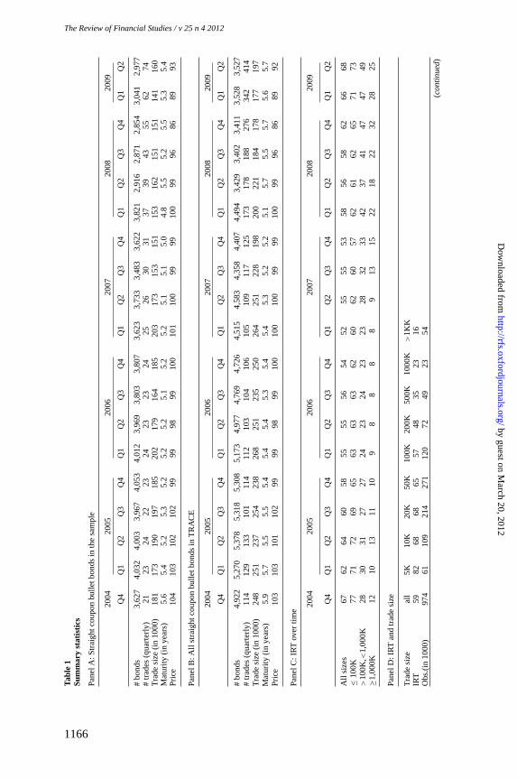
I use a sample of noncallable, nonconvertible, straight coupon bullet bondswith maturity less than thirty years. I collect information for each bondfrom Bloomberg.6 Their trading history is collected from TRACE coveringthe period from October 1, 2004, to June 30, 2009, and after filtering outerroneous trades, 10,050,090 trades are left. Error trades are filtered out usingthe approach inDick-Nielsen(2009). Summary statistics are given in PanelB in Table1. An average bond has a maturity of around five years and tradesaround 140 times each quarter, and each trade has a size of around $225,000.Trade sizes are downward-biased because trade sizes in TRACE are capped at$5,000,000 for investment-grade bonds and $1,000,000 for speculative-gradebonds. Also, while the average bond trades around 140 times each quarter, themedian bond trades only 18 times each quarter, so a small number of bondstrade often while the majority of bonds trade infrequently.
To estimate the search model outlined in the previous section, an estimateof round-trip costs in the dealer market is needed. The round-trip cost is thedifference between the price at which a dealer sells a bond to a customer andthe price at which a dealer buys a bond from a customer. Two main approachesto estimate round-trip costs exist in the literature. The first is on a given day tosubtract average buy prices from average sell prices (Hong and Warga 2000;Chakravarty and Sarkar 2003). The second is a regression-based methodologyin which each transaction price is regressed on a benchmark price and abuy/sell indicator (Schultz 2001; Bessembinder, Maxwell, and Venkataraman2006; Goldstein, Hotchkiss, and Sirri 2007; Edwards, Harris, and Piwowar2007). However, both approaches require a buy/sell indicator for each trade,which is not publicly available for the period up to October 2008. I estimatebid-ask spreads by a different procedure, which I describe below.
The methodology for estimating round-trip costs in this article is based onwhat I denoteimputed roundtrip trades(IRT). IRTs are based on a situationthat occurs with some regularity: A bond that does not trade for hours ordays suddenly has two or three trades with the same volume within, say, fiveminutes. Such trades are likely part of a pre-matched arrangement in which adealer has matched a buyer and seller. Once there is a match, a trade betweenthe seller and the dealer and a trade between the buyer and the dealer are carried
6 Moreprecisely, I require for each bond a “no” in the fields “callable” and “convertible” and a “yes” in the fields“fixed” and “bullet.” Approximately 5% of all bonds are convertible, 50% callable,80% fixed, and 50% bullet.
1165
by guest on March 20, 2012
http://rfs.oxfordjournals.org/D
ownloaded from
TheReview of Financial Studies / v 25 n 4 2012
Tabl
e1
Sum
mar
yst
atis
tics
Pan
elA
:Str
aigh
tcou
pon
bulle
tbon
dsin
the
sam
ple
2004
2005
2006
2007
2008
2009
Q4
Q1
Q2
Q3
Q4
Q1
Q2
Q3
Q4
Q1
Q2
Q3
Q4
Q1
Q2
Q3
Q4
Q1
Q2
#bo
nds
3,62
74,
032
4,00
33,
967
4,05
34,
012
3,96
93,
803
3,80
73,
623
3,73
33,
483
3,62
23,
821
2,91
62,
871
2,85
43,
041
2,97
7#
trad
es(q
uart
erly
)21
2324
2223
2423
2324
2526
3031
3739
4355
6274
Tra
desi
ze(in
1000
)18
117
319
019
718
520
217
916
418
520
317
315
315
115
316
215
115
114
116
0M
atur
ity(in
year
s)5.
65.
45.
25.
35.
25.
25.
25.
15.
25.
25.
15.
15.
04.
85.
55.
25.
55.
35.
4P
rice
104
103
102
102
9999
9899
100
101
100
9999
100
9996
8689
93
P ane
lB:A
llst
raig
htco
upon
bulle
tbon
dsin
TR
ACE
2004
2005
2006
2007
2008
2009
Q4
Q1
Q2
Q3
Q4
Q1
Q2
Q3
Q4
Q1
Q2
Q3
Q4
Q1
Q2
Q3
Q4
Q1
Q2
#bo
nds
4,92
25,
270
5,37
85,
318
5,30
85,
173
4,97
74,
769
4,72
64,
515
4,58
34,
358
4,40
74,
494
3,42
93,
402
3,41
13,
528
3,52
7#
trad
es(q
uart
erly
)11
412
913
310
111
411
210
310
410
610
510
911
712
517
317
818
827
634
241
4T
rade
size
(in10
00)
248
251
237
254
238
268
251
235
250
264
251
228
198
200
221
184
178
177
197
Mat
urity
(inye
ars)
5.9
5.7
5.5
5.5
5.4
5.4
5.4
5.3
5.4
5.4
5.3
5.2
5.2
5.1
5.7
5.5
5.7
5.6
5.7
Pric
e10
310
310
110
299
9998
9910
010
010
099
9910
099
9686
8992
P ane
lC:I
RT
over
time
2004
2005
2006
2007
2008
2009
Q4
Q1
Q2
Q3
Q4
Q1
Q2
Q3
Q4
Q1
Q2
Q3
Q4
Q1
Q2
Q3
Q4
Q1
Q2
All
size
s67
6264
6058
5555
5654
5255
5553
5856
5862
6668
≤10
0K77
7172
6965
6363
6362
6062
6057
6261
6265
7173
>10
0K, <
1,00
0K28
3031
2727
2423
2423
2328
3233
4237
4147
4749
≥1,
000K
1210
1311
109
88
88
913
1522
1822
3228
25
Pane
lD:I
RT
and
trad
e siz
e
Tra
desi
zeal
l5K
10K
20K
50K
100K
200K
500K
1000
K>
1KK
IRT
5982
6868
6557
4835
2316
Obs
.(in
1000
)97
461
109
214
271
120
7249
2354
(co
ntin
ue
d)
1166
by guest on March 20, 2012
http://rfs.oxfordjournals.org/D
ownloaded from
TheSame Bond at Different Prices: Identifying Search Frictions and Selling Pressures
Tabl
e1
Con
tinue
d
Pan
elE
:IR
Tan
dmat
urity
Mat
urity
all
0–0.
5y0.
5–1y
1–2y
2–3y
3–4y
4–5y
5–7y
7–10
y10
–30y
IRT
5926
3444
4857
5768
7210
3O
bs.(
in10
00)
974
3777
145
126
126
114
118
120
110
Pane
lF:n
umbe
rof
IRT
trad
esou
toft
otal
num
ber
of trad
es
#tr
ades
all
12
34
5–6
7–8
9–10
11–1
516
–20
21–3
031
–40
41–5
051
–100>
100
%IR
T22
046
4333
3229
2724
2118
1513
116
Bon
dda
ys(in
1000
)14
3734
130
217
511
514
184
5784
4442
2011
166
Pane
lG:v
olum
eof
IRT
trad
esou
toft
otal
vol
ume
#tr
ades
all
12
34
5–6
7–8
9–10
11–1
516
–20
21–3
031
–40
41–5
051
–100>
100
%IR
T13
019
1414
1414
1413
1313
1312
1212
Bon
dda
ys(in
1000
)14
3734
130
217
511
514
184
5784
4442
2011
166
Pane
lAsh
ows
sum
mar
yst
atis
tics
for
the
bond
sin
the
sam
ple.
Pan
elB
show
ssu
mm
ary
stat
istic
sfo
ral
lstr
aigh
tco
upon
bulle
tbo
nds
inT
RA
CE
.P
anel
Csh
ows
aver
age
roun
d-tr
ipco
sts
(mea
sure
dby
IRT
)in
cent
sov
ertim
e.P
anel
Dsh
ows
aver
age
roun
d-tr
ipco
sts
ince
nts
asa
func
tion
oftr
ade
size
.P
anel
Esh
ows
aver
age
IRT
ince
nts
asa
func
tion
ofbo
ndm
atur
ity.
InP
anel
sF
and
G,a
bond
day
isde
fined
asa
day
for
abo
ndw
here
ther
eis
atle
asto
netr
ade,
and
the
bond
days
are
sort
edac
cord
ing
toth
enu
mbe
rof
trad
esoc
curr
ing
onth
atda
y.O
utof
the
tota
lnum
ber
ofbo
ndtr
ades
ona
bond
day,
Pan
elF
show
sth
efr
actio
nof
trad
esth
atar
epa
rtof
anIR
T.F
orex
ampl
e,th
ere
are
302,
000
obse
rvat
ions
ofa
bond
trad
ing
two
times
ina
day,
and
outo
fthe
604,
000
tran
sact
ions46
%ar
epa
rtof
anIR
T.P
anel
Gsh
ows
the
frac
tion
ofvo
lum
eth
atis
part
ofan
IRT.
For
exam
ple,
ther
ear
e30
2,00
0ob
serv
atio
nsof
abo
ndtr
adin
gtw
otim
esin
ada
y,an
dou
toft
heto
talv
olum
eof
the
604,
000
tran
sact
ions
,19
%is
part
ofan
IRT.
The
sam
ple
bond
sar
est
raig
htco
upon
bulle
tbon
ds,a
ndth
esa
mpl
epe
riod
isO
ctob
er1,
2004
,to
June
30,2
009.
1167
by guest on March 20, 2012
http://rfs.oxfordjournals.org/D
ownloaded from

TheReview of Financial Studies / v 25 n 4 2012
out. If a second dealer is involved in the pre-matching, there is also a tradebetween the two dealers. Therefore, for a given bond on a given day, if thereare exactly two or three trades for a given volume and they occur within fifteenminutes, I define these trades to be part of an IRT. In an IRT, the highest priceis assumed to be an investor buying from a dealer, the lowest price assumedto be an investor selling to a dealer, and the investor round-trip cost to be thehighest minus the lowest price. I delete IRTs with a zero round-trip cost fromthe sample.7 Beginning in November 2008, buy/sell indicators are available,which allows me to check the accuracy of IRTs for this subsample (shownin Appendix C). Appendix C shows that although IRTs tend to underestimateround-trip costs, the empirical results are robust to this bias.
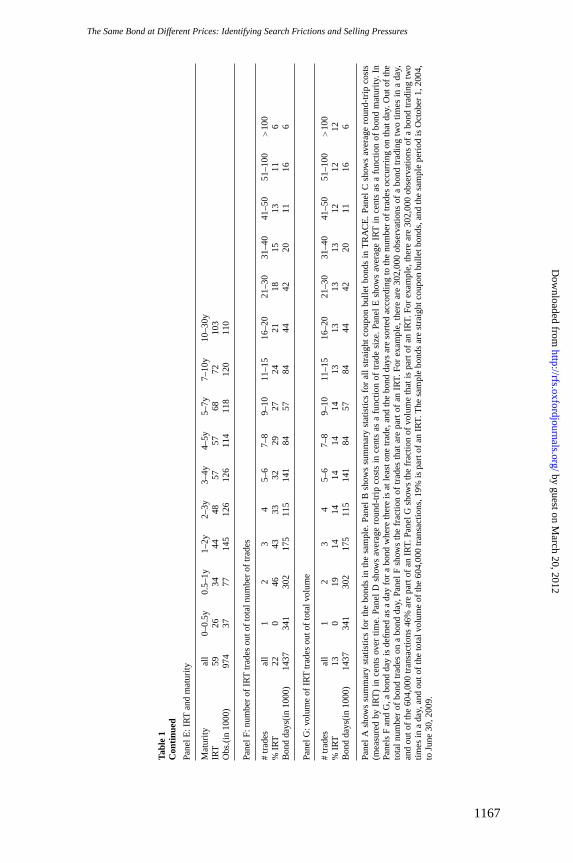
Of the 10,050,090 trades in the full sample, 2,159,447 are part of IRTs,resulting in a total of 973,600 IRTs. Panel A in Table1 shows summarystatistics for the subsample of data consisting of IRTs. We see that averagetrade sizes are slightly lower compared with the full sample, average maturityis roughly the same, and the number of quarterly trades decreases from anaverage of around 140 to around 30. Approximately 20% of the bonds dropout of the sample. Panels F and G address whether IRTs occur mostly in theliquid or illiquid segment of the corporate bond market. Panel F shows thatmost of the IRT trades are in bonds that have few trades each day. However,Panel G shows that the total fraction of trade volume that is captured by IRTsis almost the same across bonds that trade frequently and infrequently. Thus,IRTs capture transaction costs for both liquid and illiquid bonds.
Summary statistics of trading costs using IRTs are given in Table1, PanelsC–E. Panel D shows that the average transaction cost is 59 cents and isdecreasing as a function of trade size. This is consistent with findings inSchultz (2001), Chakravarty and Sarkar(2003), andEdwards, Harris, andPiwowar (2007). Transaction costs are increasing in maturity, as Panel Eshows. Costs are around four times as large for long maturities comparedwith short maturities. Finally, Panel C shows that average transaction costsdecrease from 2004 to 2006 and increase during the subprime crisis 2007–2009. There are significant differences in the time-series pattern for large andsmall trades. Transaction costs for small trades are relatively stable during thesample period. Costs for large trades increase with a factor of 4 from the firstquarter in 2007 to the fourth quarter in 2008.
The main point in this article is that price differences between small andlarge trades identify periods of selling pressure, and this is so for both buyand sell prices. The onset of the subprime crisis caused liquidity in the U.S.corporate bond market to dry up (Bao, Pan, and Wang 2011; Dick-Nielsen,Feldhutter, and Lando forthcoming), and Table2 shows summary statistics for
7 IRTs are closely related toGreen, Hollifield, and Schurhoff’s (2007) “immediate matches.” An “immediatematch” is a pair of trades where a buy from a customer is followed by a sale to a customer in the same bondfor the same par amount on the same day with no intervening trades in that bond. However, since there is noinformation about the sides in the transactions in the TRACE database, “immediate trades” cannot be calculated.
1168
by guest on March 20, 2012
http://rfs.oxfordjournals.org/D
ownloaded from
TheSame Bond at Different Prices: Identifying Search Frictions and Selling Pressures
Table 2Differences in prices for small and large trades
Panel A: Small buy – large buy(early)
0–2y 2–5y 5–7y 7–30y Average
0–100K 0 0 0 0 0100K–250K −1 7 13 11 8250K–500K 3 15 26 26 17500–1,000K 2 22 36 35 24>1,000K 8 33 35 52 32
Average 3 19 28 31
Panel B: Small sell – large sell(early)
0–2y 2–5y 5–7y 7–30y Average
0–100K 0 0 0 0 0100K–250K −15 −16 −18 −31 −20250K–500K −17 −22 −23 −39 −25500–1,000K −23 −22 −20 −42 −27>1,000K −21 −12 −21 −21 −19
Average −19 −18 −20 −33
Panel C: Buy-diff(early) – buy-diff(late)
0–2y 2–5y 5–7y 7–30y Average
0–100K 0 0 0 0 0100K–250K −7 −13 −7 −16 −11250K–500K −19 −23 −28 −32 −25500–1,000K −33 −30 −33 −46 −36>1,000K −29 −31 −46 −58 −41
Average −22 −24 −29 −40
Panel D: Sell-diff(early) – sell-diff(late)
0–2y 2–5y 5–7y 7–30y Average
0–100K 0 0 0 0 0100K–250K −17 −23 −22 −34 −24250K–500K −30 −36 −41 −51 −40500–1,000K −44 −40 −47 −64 −49>1,000K −40 −37 −47 −65 −47
Average −33 −34 −39 −54
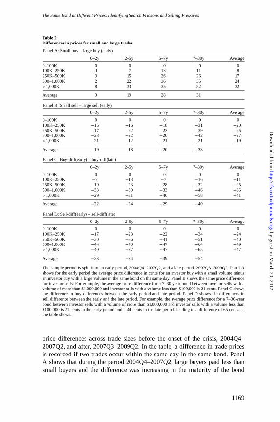
Thesample period is split into an early period, 2004Q4–2007Q2, and a late period, 2007Q3–2009Q2. Panel Ashows for the early period the average price difference in cents for an investor buy with a small volume minusan investor buy with a large volume in the same bond on the same day. Panel B shows the same price differencefor investor sells. For example, the average price difference for a 7–30-year bond between investor sells with avolume of more than$1,000,000and investor sells with a volume less than$100,000is 21 cents. Panel C showsthe difference in buy differences between the early period and late period. Panel D shows the differences insell difference between the early and the late period. For example, the average price difference for a 7–30-yearbond between investor sells with a volume of more than$1,000,000and investor sells with a volume less than$100,000is 21 cents in the early period and−44 cents in the late period, leading to a difference of 65 cents, asthe table shows.
price differences across trade sizes before the onset of the crisis, 2004Q4–2007Q2, and after, 2007Q3–2009Q2. In the table, a difference in trade pricesis recorded if two trades occur within the same day in the same bond. PanelA shows that during the period 2004Q4–2007Q2, large buyers paid less thansmall buyers and the difference was increasing in the maturity of the bond
1169
by guest on March 20, 2012
http://rfs.oxfordjournals.org/D
ownloaded from
TheReview of Financial Studies / v 25 n 4 2012
and trade size. For example, the selling price for a long-maturity bond wason average 52 cents higher for a trade of at least $1,000,000 compared with atrade of $100,000 or less. Similarly, Panel B shows that large investors sold athigher prices than small investors, and we see that the difference increased inbond maturity and trade size, although the pattern is less pronounced than forinvestor buy transactions.
The results in Panels A and B of Table2 are not surprising given that transac-tion costs increase in bond maturity and decrease in trade size. More strikingly,Panels C and D show how price differences across trade sizes changed after theonset of the subprime crisis. While the average selling price of a long-maturitybond was 21 cents higher in a large trade compared with a small trade beforethe subprime crisis, Panel D shows that this decreased by 65 cents after theonset of the crisis, such that the average selling price in large trades was now 44cents lower than in a small trade. We see from Panels C and D that the impactof the subprime crisis on price differences is increasing in bond maturity andtrade size. In addition, the impact is similar in buys and sells.8
Overall, Panels C and D show that price differences change systematicallyduring the subprime crisis and the size of the change depends on both bondmaturity and trade size.
4. Estimation Methodology
Liquidity risk and credit risk are hard to empirically disentangle, sinceprices decrease in response to an increase in either of them. Assuming thatlarge traders are more sophisticated than small traders, the model in thisarticle predicts that prices of large traders react stronger to selling pressure thanthose of small traders. Therefore, a liquidity shock can be identified throughthe relation of small trades versus large trades.
A simple approach to identify liquidity shocks would be to calculate pricedifferences between small and large trades, where the cutoff between smalland large is some chosen dollar value. This approach is problematic for severalreasons. First, information in trades of different sizes is ignored. For example,if the cutoff is $500,000, then any price differences between trades in the sizerange $250,000–500,000 and $0–100,000 are not used in inferring liquidityshocks. As Panels C and D in Table2 show, there is a significant amount ofinformation in those price differences. Second, maturity effects are ignored.When following the same bond over time, the maturity of the bond shortens,and this has an effect on the impact of liquidity shocks on price differences,as Panels C and D show. Third, many bonds trade infrequently, so whenconstructing the measure, there are many missing observations over time.
8 Althoughnot shown, the pattern for median price differences is very similar and in some cases more pronouncedcompared with the pattern for mean price differences, so the results are not due to a small number of extremeobservations.
1170
by guest on March 20, 2012
http://rfs.oxfordjournals.org/D
ownloaded from

TheSame Bond at Different Prices: Identifying Search Frictions and Selling Pressures
To overcome the limitations of the simple approach, I structurally estimatethe search model in Section2. In the structural approach, information isextracted from the whole cross-section of trade sizes. The longer maturity abond has, the stronger is the price reaction to selling pressure. In the structuralapproach, this is taken into account when extracting information from bondtrades. And missing observations are easy to handle.
In the estimation, I fit the model to demeaned prices. By demeaning, effectsdue to credit risk or other fundamental effects are “filtered out,” while cross-sectional differences in trade prices identify liquidity effects. Any bid or askprices for a given bond on a given day are demeaned with the average of allbid and ask prices for this bond on this day. All prices refer to trades that arepart of IRTs. That is, if there areNtb IRTs on bondb on dayt , and Atbi isthe i th ask price andBtbi thecorresponding bid price, the demeaned ask priceis defined asAtbi − ABtb and demeaned bid price asBtbi − ABtb, whereABtb = 1
2Ntb
∑Ntbi =1(Atbi + Btbi ).
Let Θ be a vector with the parameters of the model, ands be a shocksize between 0 and 1 defined in Definition2.1. For dayt and bondb, alldemeaned bid and ask prices are denotedP1
tb, P2tb, ..., P2Ntb−1
tb , P2Ntbtb (the
sortingdoes not matter). With a shock size ofs on dayt , the demeaned fittedpricesP1
tb(Θ, st ), P2tb(Θ, st ), . . ., P2Ntb−1
tb (Θ, st ), P2Ntbtb (Θ, st ) arecalculated
using Theorem2.2. I assume that fitting errors are independent and normallydistributed with zero mean and a standard deviation that depends on thematurity of the bond
Pitb − Pi
tb(Θ, st ) ∼ N(0,wtbσ2),
wtb = max(1,Ttb),
whereTtb is the maturity of bondb on dayt . The choice ofwtb is motivated bythe fact that pricing errors tend to increase with maturity, while at the same timeexcessive influence of prices for bonds with maturity close to zero is avoided.With this error specification, we have that
ε itb(Θ, st ) =
Pitb − Pi
tb(Θ, st )√
wtb∼ N(0,σ 2).
Thelikelihood function is given as
− 2 logL(Θ|Y) =1
σ 2
T∑
t=1
Nb∑
b=1
2Ntb∑
i =1
ε itb(Θ, st (Θ))2
+T∑
t=1
Nb∑
b=1
2Ntb∑
i =1
[log(σ 2) + 2π], (2)
whereNb is the number of bonds in the sample andst (Θ) is defined as
1171
by guest on March 20, 2012
http://rfs.oxfordjournals.org/D
ownloaded from

TheReview of Financial Studies / v 25 n 4 2012
st (Θ) = arg minξ
∑
all daysu thatbelongto samemonth as dayt
Nb∑
b=1
2Nub∑
i =1
ε iub(Θ, ξ)2. (3)
Thatis, I assume that all days in a month experience the same liquidity shock,and for a given parameter vectorΘ this shock is found to be minimizing thesum of squared pricing errors for that month’s prices. The approach is similarto that ofJarrow, Li, and Zhao(2007), and a more detailed discussion aboutthe estimation procedure can be found there. The estimation jointly estimatesthe parameter vectorΘ and a time series of monthly liquidity shocks.
I use trade size as a proxy for investor sophistication. Specifically, there aresix investor classes that differ in their search intensityρ, and they trade in parvalues of $0–10,000, $10,000–50,000, $50,000–100,000, $100,000–500,000,$500,000–1,000,000, and more than $1,000,000.9 Goldstein,Hotchkiss, andSirri (2007) andBessembinder, Kahle, Maxwell, and Xu(2009) find that tradessmaller than $100,000 are mainly retail trades and trades bigger than $100,000are predominantly institutional trades. So, one interpretation of a small trader isthat of an unsophisticated retail investor, while a large trader is a sophisticatedinstitutional investor.Lagos and Rocheteau(2009) andGarleanu(2009) easethe restriction that asset holdings are zero or one. They find that there is apositive relationship between trade size and sophistication, as measured bysearch intensity. The restriction on asset holdings does not allow for such apositive relationship here, but I control for this empirically by using tradesize as a proxy for investor sophistication. For future research, it would beinteresting to exploit trade size information in the estimation even more byallowing for arbitrary asset holdings.
There are a number of parameters in the model for which historical estimatesare available. The riskless rate is set tor = 0.05, which is close to the averageten-year swap rate of 4.94% in the estimation period. The bond coupon is set toseven, close to the average coupon rate in the sample period, and face value toF = 100. The default intensity is set toλD = 0.012,and the recovery rate onthe bond in case of default is set to 42% such thatf = 0.58. The last two areaverages for the period 1994–2008 (see Exhibit 26 and 45 inMoody’s 2009). Icould let the riskless rate be time-varying in the estimation, allow for differentdefault intensities across rating, and let the bond coupon reflect each bond’sactual coupon. Since the effect on the estimation results of doing so is smallbecause I fit to demeaned prices and not to price levels, I choose the moreparsimonious approach. Finally, I setω = 0.0001. The parameters to estimateareΘ = (δ, λ, π, z, ρ1, ρ2, ρ3, ρ4, ρ5, ρ6).
9 Table1 shows that average trade size decreases from$180,000to 200,000 to approximately$150,000duringthe subprime crisis (see Dick-Nielsen, Feldhutter, and Lando forthcoming for a further discussion). This mightinfluence the results, but the effect is likely to be small because the differences in the trade size of investor classesare large.
1172
by guest on March 20, 2012
http://rfs.oxfordjournals.org/D
ownloaded from

TheSame Bond at Different Prices: Identifying Search Frictions and Selling Pressures
5. Empirical Results
5.1 Parameter estimates and model fitTable3 shows the parameter estimates. We see that search intensities increaseas trade size increases, so more sophisticated investors trade in larger sizes.The most unsophisticated investors (trading in sizes between 0 and $5,000)have a search intensity of 40. This implies that they need around a week onaverage before they find a dealer with whom to trade with. This can be viewedas the time it takes a nonprofessional to learn how to trade in the corporatebond market, keep up to date about information relevant for trading, and findan alternative dealer in case his preferred one gives him uncompetitive prices.The most sophisticated investors (trading sizes of more than $1,000,000)have a search intensity of 372, implying that it takes half a day to completetrades of large size. The productλπ = 0.33 implies that, without aggregateliquidity shocks, it is a rare event for a corporate bond investor to be hit bya liquidity shock; it occurs on average once every three years. A liquidity-shocked investor remains shocked for about three months sinceλ = 3.58. Theestimated bargaining power of dealers ofz = 0.97 shows that dealers are in astrong bargaining position relative to investors.
Panel A of Table4 shows fitted round-trip costs. The model underestimatesround-trip costs for the smallest trades, while round-trip costs for large tradesare matched well. In particular, the strong negative relation between trade sizeand trading costs is captured. In Panel B, we see that the model replicatesthe positive relation between round-trip costs and bond maturity although costsare underestimated for long-maturity bonds.Chakravarty and Sarkar(2003)point to increased interest rate risk as a possible explanation for the positiverelation between trading costs and maturity. This analysis shows that to alarge extent the relation can be explained by better outside options of investorstrading short maturity bonds.
Panels C and D of Table4 show the change in price differences betweensmall and large trades after the onset of the subprime crisis. Remember thatthese differences identify selling pressure in the model. Compared with actualchanges in Panels C and D of Table2, we see that the model largely capturesthe size of the change for both buy and sell transactions. Also, the modelcaptures the relation between price difference changes and bond maturity and
Table 3Parameterestimates
δ λ π z ρ1 ρ2 ρ3 ρ4 ρ5 ρ6
2.911(0.003)
3.580(0.090)
0.092(0.013)
0.970(0.001)
40(1.1)
38(1.0)
50(0.9)
101(1.7)
278(23.7)
372(8.5)
This table shows estimated parameters of the search model. Model parameters are estimated by maximumlikelihood, and standard errors are calculated using the outer product of gradients estimator. Corporate bonddata used in estimation are transactions from TRACE for the period October 1, 2004, to June 30, 2009.
1173
by guest on March 20, 2012
http://rfs.oxfordjournals.org/D
ownloaded from

TheReview of Financial Studies / v 25 n 4 2012
Table 4Estimated round-trip costs and price differences
Panel A: Trade size [Panel D in Table1]
0–10K 11–50K 51–100K 101–500K 501–1000K >1000K
54 54 47 38 21 19
Panel B: Maturity [Panel E in Table1]
0–2m 2m–4m 4–6m 6m–1y 1–5y 5–30y18 30 37 43 50 52
Panel C: Buy-diff(early) - buy-diff(late) [Panel C in Table2]
0–2y 2–5y 5–7y 7–30y Average
0–100K 0 0 0 0 0100K–250K −15 −22 −22 −24 −21250K–500K −21 −28 −27 −29 −27500–1,000K −32 −43 −42 −46 −41>1,000K −33 −43 −44 −46 −42
Average −26 −34 −34 −36
Panel D: Sell-diff(early) - sell-diff(late) [Panel D in Table2]
0–2y 2–5y 5–7y 7–30y Average
0–100K 0 0 0 0 0100K–250K −15 −22 −22 −24 −21250K–500K −20 −29 −28 −31 −27500–1,000K −32 −44 −43 −46 −41>1,000K −33 −43 −44 −46 −42
Average −25 −34 −34 −37
This table reports model-fitted round-trip costs and price differences. Panel A compares with Panel D in Table1, Panel B compares with Panel E in Table1, Panel C compares with Panel C in Table2, and Panel D compareswith Panel D in Table2.
tradesize. Thus, the model captures how price differences change along bondmaturity and trade size, and it does so for both buy and sell prices.
The following calculations provide an estimate of the additional cost due tosearch that investors in the corporate bond market incur compared with that ofthe Treasury market. The average maturity in the data sample is 5.5 years, soa five-year bond is the most representative bond for the corporate market. Anestimate of the average bid-ask spread as a percentage of par value of a five-year bond in the Treasury market is 0.012% according toFleming(2003). Foran average investor, i.e. an investor with an average search intensity, the corre-sponding estimate for a five-year bond in the corporate bond market is 0.343%according to the parameter estimates and Equation (1). Thus, an estimate of thecost of search on a trade in the corporate bond market relative to the Treasurymarket is half the round-trip cost, 0.166%. The yearly trading volume in thecorporate bond market was $4,284 billion in 2009.10 So, an estimate of the
10 Average daily volume in the U.S. corporate bond market was$16.8 billion according to the Securities andFinancial Markets Association (www.sifma.org), so yearly was 255*$16.8billion.
1174
by guest on March 20, 2012
http://rfs.oxfordjournals.org/D
ownloaded from

TheSame Bond at Different Prices: Identifying Search Frictions and Selling Pressures
additionalyearly costs investors bear in the corporate bond market comparedwith the Treasury market is $4,284 billion∗0.166%= $7.1 billion.
5.2 Selling pressureIn response to a liquidity shock, prices decrease and slowly return to theirequilibrium level as time passes. In previous literature, selling pressure is iden-tified through this pattern. However, it is difficult to disentangle price effectsdue to a liquidity shock from price effects due to changes in fundamentals.For example, a downgrade might lead to selling pressure, but there is also aninformational effect of the downgrade.
In this article, selling pressure is identified by the cross-sectional variation inprices. For example, assume that the difference in bid prices in a bond betweenlarge trades and small trades in steady state is 20 cents. If this decreases to10 cents one month, there is a liquidity shock that month. If it decreases to,say,−10 cents, there is an even larger liquidity shock. The same pattern inask prices identifies liquidity shocks, and the estimation procedure uses theinformation in both bid and ask prices. Note that the shock size is identifiedonly through multiple observations of bid and ask prices in a bond on agiven day for investors with different search intensities. If investors were notsorted according to sophistication and there instead was a single representativeinvestor, shocks could not be identified.
Figure3 graphs the estimated selling pressure. A 95% confidence intervalis bootstrapped according toBradley(1981).11 In the first part of the sampleperiod, there is one modest shock occurring. GM and Ford were downgradedto junk bond status in May 2005, causing a test for the corporate bond marketbecause of the amount of GM/Ford debt outstanding. To examine the effect ofthe downgrade on the corporate bond market more closely, Figure4 shows theselling pressure for Ford bonds, GM bonds, and the rest of the corporate bondmarket around this period.
In late 2004, S&P downgraded GM to BBB–, the last rating notch before ajunk rating, and the graph shows some selling pressure in this period consistentwith evidence inAcharya, Schaefer, and Zhang(2008). Many bond investorsand asset managers are restricted to invest in only investment-grade bonds,so they started to sell off GM bonds, anticipating the future downgrade tojunk. BIS (2005) write, “The downgrade had long been anticipated and soasset managers had ample opportunity to adjust their portfolios. Since mid-2003, the automakers’ spreads had been trading closer to speculative-gradeissuers than those on other BBB-rated issuers.” As it became increasinglylikely that especially GM would be downgraded, selling pressure increased inthe beginning of 2005. Interestingly, selling pressure temporarily decreasedin February 2005. On January 24, 2005, Lehman announced that it would
11 For each month, the bootstrapped standard errors are based on 500 simulated datasets.
1175
by guest on March 20, 2012
http://rfs.oxfordjournals.org/D
ownloaded from
The Review of Financial Studies / v 25 n 4 2012
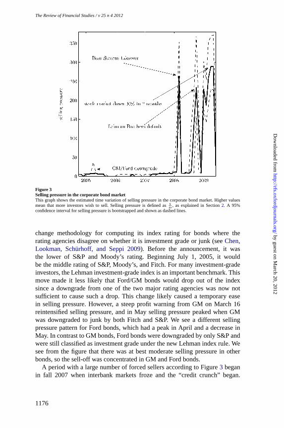
Figure 3Selling pressure in the corporate bond marketThis graph shows the estimated time variation of selling pressure in the corporate bond market. Higher valuesmean that more investors wish to sell. Selling pressure is defined ass
ω , as explained in Section2. A 95%confidence interval for selling pressure is bootstrapped and shown as dashed lines.
change methodology for computing its index rating for bonds where therating agencies disagree on whether it is investment grade or junk (seeChen,Lookman, Schurhoff, and Seppi 2009). Before the announcement, it wasthe lower of S&P and Moody’s rating. Beginning July 1, 2005, it wouldbe the middle rating of S&P, Moody’s, and Fitch. For many investment-gradeinvestors, the Lehman investment-grade index is an important benchmark. Thismove made it less likely that Ford/GM bonds would drop out of the indexsince a downgrade from one of the two major rating agencies was now notsufficient to cause such a drop. This change likely caused a temporary easein selling pressure. However, a steep profit warning from GM on March 16reintensified selling pressure, and in May selling pressure peaked when GMwas downgraded to junk by both Fitch and S&P. We see a different sellingpressure pattern for Ford bonds, which had a peak in April and a decrease inMay. In contrast to GM bonds, Ford bonds were downgraded by only S&P andwere still classified as investment grade under the new Lehman index rule. Wesee from the figure that there was at best moderate selling pressure in otherbonds, so the sell-off was concentrated in GM and Ford bonds.
A period with a large number of forced sellers according to Figure3 beganin fall 2007 when interbank markets froze and the “credit crunch” began.
1176
by guest on March 20, 2012
http://rfs.oxfordjournals.org/D
ownloaded from

The Same Bond at Different Prices: Identifying Search Frictions and Selling Pressures
Figure 4Selling pressure in GM and Ford bonds around their downgrade to junkThis graph shows the time variation in selling pressure in GM bonds, Ford bonds, and the rest of the corporatebond market around the downgrade of GM and Ford to junk in 2005. They-axis shows selling pressure, andhigher values correspond to more sellers.
However, the first signs of selling pressure appeared already in April 2007when the subprime mortgage crisis spilled over into the corporate bond market(Brunnermeier 2009). Figure3 shows a large shock in March 2008.BIS (2008)write, “Turmoil in credit markets deepened in early March...tightening repohaircuts caused a number of hedge funds and other leveraged investors tounwind existing positions. As a result, concerns about a cascade of margincalls and forced asset sales accelerated the ongoing investor withdrawal fromvarious financial markets. In the process, spreads on even the most highly ratedassets reached unusually wide levels, with market liquidity disappearing acrossmost fixed income markets.” A liquidity squeeze on Bear Stearns caused atakeover by JPMorgan on March 17. The Federal Reserve cut the policy rateby 75 basis points, and “(t)hese developments appeared to herald a turningpoint in the market...with investors increasingly adopting the view that variouscentral bank initiatives aimed at reliquifying previously dysfunctional marketswere gradually gaining traction” (BIS 2008). The selling pressure in May 2008is very low compared with a few months earlier. According toBIS (2008), “By
1177
by guest on March 20, 2012
http://rfs.oxfordjournals.org/D
ownloaded from

TheReview of Financial Studies / v 25 n 4 2012
the end of the period in late May, the process of disorderly deleveraging hadcome to a halt, giving way to more orderly credit market conditions. Marketliquidity had improved and risk appetite increased, luring investors back intothe market.” However, this rebound of the corporate bond market was short-lived, and the model-implied liquidity shocks peaked again in September andOctober 2008. Lehman Brothers filed for bankruptcy on September 2008, oneof the biggest credit events in history, triggering a new and intensified stageof the credit crisis. At the end of 2008, there was a brief halt in sellingpressure, but in the first three months of 2009, selling pressure intensifiedagain. In this period, stock markets lost more than 30% in value. This losslikely worsened funding conditions, leading to a loss in liquidity across assetclasses as predicted byBrunnermeier and Pedersen(2009). Finally, the secondquarter of 2009 saw a decrease in the selling pressure consistent with creditspreads tightening in the period.
5.3 The credit spread puzzleOne of the most widely employed frameworks of credit risk, structural models,was developed in the seminal work ofMerton (1974). Structural models takeas given the dynamics of the value of a firm and value corporate bonds ascontingent claims on the firm value. In structural models, the spread betweenthe yield on a corporate bond and the riskless rate goes to zero as maturityshortens. However, yield spreads are typically positive, also at very shortmaturities. This has given rise to the “credit spread puzzle,” namely thatcorporate yield spreads are too high to be explained by the corporate bondissuer’s default risk (see, for example,Huang and Huang 2003; Chen, Collin-Dufresne, and Goldstein 2009). The puzzle is particularly severe at very shortmaturities. Consistent with this evidence, among others,Longstaff (2004),Longstaff, Mithal, and Neis(2005), andFeldhutter and Lando(2008) find alarge non-default component. In this section, I examine to what extent searchfrictions and selling pressures can explain this non-default component.12
I define the search premium for an investor as the midyield paid by thisinvestor in steady state minus the yield in steady state of an investor whocan instantly find a trading partner (ρ = ∞).13 This mimics a trade inthe corporate bond market versus a trade in the liquid Treasury market. Ido this for an “average” corporate bond investor, where the search intensity
12 The model in this article is related to reduced-form models of credit risk, where there is an intensity processgoverning the risk of default. Thus, it does not predict a near-zero contribution of default risk to spreads atvery short maturities as structural models. Nevertheless, the implications of search costs can be examined in themodel.
13 It is easy to show that the discounted present value of the promised payments of a bond using discount ratey is
E(∫ τT0 Ce−yt dt + e−yτT F) =
C+λT Fy+λT
whereτT is the (stochastic) maturity. Therefore the yieldy on a bond
with price P is y =C+λT F
P − λT , which is the formula used to convert prices to yields.
1178
by guest on March 20, 2012
http://rfs.oxfordjournals.org/D
ownloaded from
TheSame Bond at Different Prices: Identifying Search Frictions and Selling Pressures
is the average of all the estimated search intensities in Table3.14 For thesame “average” investor, I define the selling pressure premium as the averageestimated midyield across all months minus the average midyield across allmonths where all liquidity shocks are set to zero.
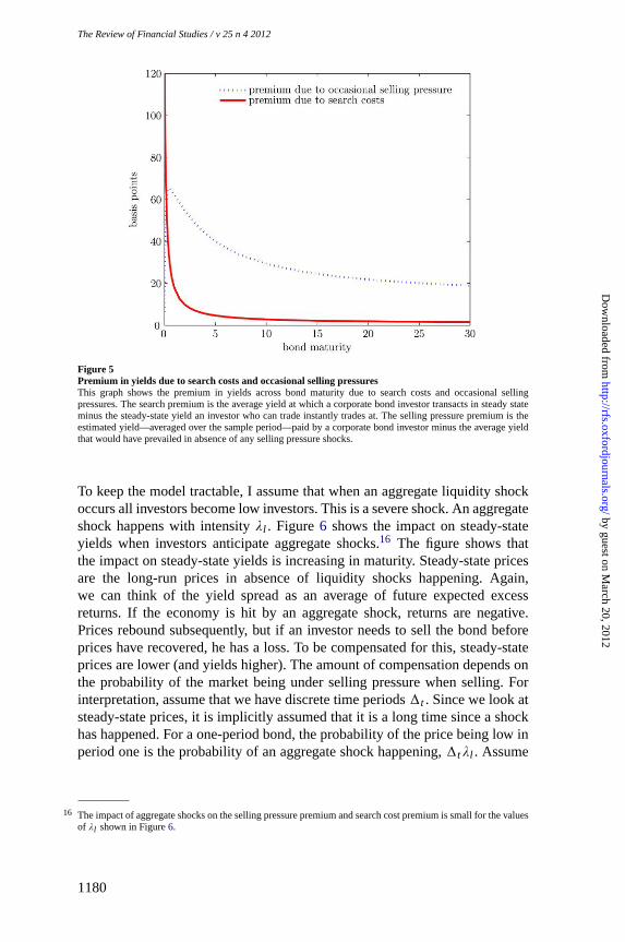
Figure 5 graphs the term structure of search premia and selling pressurepremia. The figure shows that search costs affect primarily the short end of theyield curve. The premium is more than 100 basis points for bonds with veryshort maturities (less than three weeks). For bonds with maturities of more thantwo years, the effect of search costs is in the single-digit range. There are tworeasons for the downward-sloping costs of search. First, if a liquidity-shockedinvestor owns a short-maturity bond, he is likely to be liquidity-shocked duringthe life of the bond. This means that he values the bond almost as a bond payingC − δ in coupons. So, the yield cost of holding the bond isδ. If a liquidity-shocked investor owns a long-maturity bond, he values it higher than a bondpaying couponsC − δ because he will likely switch type during the life ofthe bond. Therefore, the average yield cost of holding the bond is less thanδ. Second, if an investor owns a short-maturity bond, he has fewer tradingopportunities during the life of the bond. So, for a short-maturity bond, thealternative to trade is essentially to let the bond mature. For a long-maturitybond, the additional alternative is to look for another counterparty.
Turning to the impact of selling pressure, Figure5 shows that the averageeffect decreases as a function of maturity. The yield spread due to sellingpressure at a given maturity can be viewed as the average of future expectedexcess returns. The initial returns at the beginning of a liquidity shock are high,so for short maturity bonds all future expected excess returns are high. For longmaturity bonds, the average is over initial high returns and subsequent lowerreturns when the economy has fully recovered. Therefore, the effect is strongerfor short maturity bonds.15
For a five-year bond, the selling pressure effect is 40 basis points.Huang andHuang(2003) andLongstaff, Mithal, and Neis(2005) find the average non-default component of the five-year AAA-Treasury spread to be 50–55 basispoints. The combined effect of selling pressure and search costs is 45 basispoints in my data sample. Such comparisons should be interpreted with caredue to differences in sample periods, but the comparison does suggest that theestimated premium is close to but underestimates that reported in the literature.One reason might be that investors in the model do not recognize the possibilityof a future liquidity shock. To examine this, I solve the model in the casewhere investors anticipate future liquidity shocks. This is done in Appendix B.
14 Specifically, when I calculate the yields for an “average” investor, I setρ4 to 147 instead of 101 and look atyields for investor 4. When I calculate yields for an investor withρ = ∞, I setρ6 = ∞ insteadof 372 and lookat yields for investor 6.
15 Thepremium due to selling pressure is hump-shaped at very short maturities. This is because the rate of priceincreases for a while is higher when markets become integrated compared with immediately after the shock.
1179
by guest on March 20, 2012
http://rfs.oxfordjournals.org/D
ownloaded from
The Review of Financial Studies / v 25 n 4 2012
Figure 5Premium in yields due to search costs and occasional selling pressuresThis graph shows the premium in yields across bond maturity due to search costs and occasional sellingpressures. The search premium is the average yield at which a corporate bond investor transacts in steady stateminus the steady-state yield an investor who can trade instantly trades at. The selling pressure premium is theestimated yield—averaged over the sample period—paid by a corporate bond investor minus the average yieldthat would have prevailed in absence of any selling pressure shocks.
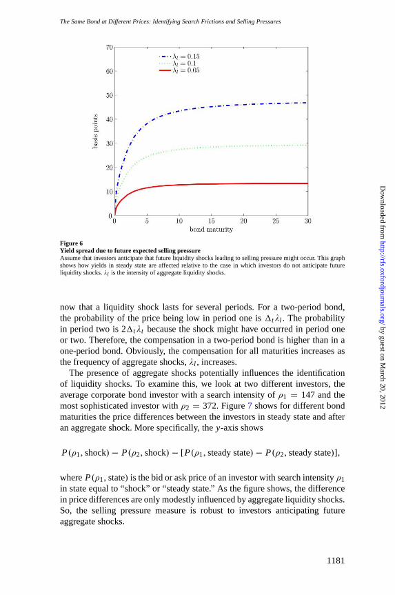
To keep the model tractable, I assume that when an aggregate liquidity shockoccurs all investors become low investors. This is a severe shock. An aggregateshock happens with intensityλl . Figure6 shows the impact on steady-stateyields when investors anticipate aggregate shocks.16 The figure shows thatthe impact on steady-state yields is increasing in maturity. Steady-state pricesare the long-run prices in absence of liquidity shocks happening. Again,we can think of the yield spread as an average of future expected excessreturns. If the economy is hit by an aggregate shock, returns are negative.Prices rebound subsequently, but if an investor needs to sell the bond beforeprices have recovered, he has a loss. To be compensated for this, steady-stateprices are lower (and yields higher). The amount of compensation depends onthe probability of the market being under selling pressure when selling. Forinterpretation, assume that we have discrete time periods1t . Since we look atsteady-state prices, it is implicitly assumed that it is a long time since a shockhas happened. For a one-period bond, the probability of the price being low inperiod one is the probability of an aggregate shock happening,1tλl . Assume
16 The impact of aggregate shocks on the selling pressure premium and search cost premium is small for the valuesof λl shown in Figure6.
1180
by guest on March 20, 2012
http://rfs.oxfordjournals.org/D
ownloaded from
The Same Bond at Different Prices: Identifying Search Frictions and Selling Pressures
Figure 6Yield spread due to future expected selling pressureAssume that investors anticipate that future liquidity shocks leading to selling pressure might occur. This graphshows how yields in steady state are affected relative to the case in which investors do not anticipate futureliquidity shocks.λl is the intensity of aggregate liquidity shocks.
now that a liquidity shock lasts for several periods. For a two-period bond,the probability of the price being low in period one is1tλl . The probabilityin period two is 21tλt because the shock might have occurred in period oneor two. Therefore, the compensation in a two-period bond is higher than in aone-period bond. Obviously, the compensation for all maturities increases asthe frequency of aggregate shocks,λl , increases.
The presence of aggregate shocks potentially influences the identificationof liquidity shocks. To examine this, we look at two different investors, theaverage corporate bond investor with a search intensity ofρ1 = 147 and themost sophisticated investor withρ2 = 372. Figure7 shows for different bondmaturities the price differences between the investors in steady state and afteran aggregate shock. More specifically, they-axis shows
P(ρ1, shock)− P(ρ2, shock)− [ P(ρ1, steady state) − P(ρ2, steady state)],
whereP(ρ1, state)is the bid or ask price of an investor with search intensityρ1in state equal to “shock” or “steady state.” As the figure shows, the differencein price differences are only modestly influenced by aggregate liquidity shocks.So, the selling pressure measure is robust to investors anticipating futureaggregate shocks.
1181
by guest on March 20, 2012
http://rfs.oxfordjournals.org/D
ownloaded from

The Review of Financial Studies / v 25 n 4 2012
Figure 7Identification of selling pressure in presence of aggregate liquidity shocksThis graph shows how selling pressure can still be identified in presence of aggregate liquidity shocks. Pricedifferences are graphed for an average corporate bond investor (search intensityρ1 = 147) and the mostsophisticated investor in the sample (ρ2 = 372). On they-axis, we have the price difference between the twoinvestors after a shock minus the price difference in steady state.λl is the intensity of aggregate liquidity shocks.
6. Conclusion
For over-the-counter traded assets, I propose a measure that identifies whenasset prices are affected by selling pressure—namely, the price differencebetween small and large trades. In a model capturing the search-and-bargainingfeatures in over-the-counter markets, the connection between the measure andselling pressure is derived. I structurally estimate the model using U.S. cor-porate bond transaction data from October 2004 to June 2009. The estimationprovides new insights into two periods of selling pressure: the downgradeof GM/Ford and the subprime crisis. Also, the effect of trading frictions andselling pressures on the term structure of corporate bond illiquidity premia isexamined.
The analysis raises a number of questions. Here, the U.S. corporate bondmarket is examined on an aggregate level. An extension is to understand thecross-sectional variation in selling pressure across bonds. The U.S. municipalbond market is another illiquid over-the-counter market with transaction dataavailable, and the nature of its illiquidity can be studied using the approach inthis article. Even in highly liquid markets, search frictions matter, asAshcraftand Duffie(2007) show for the federal funds market, and the Treasury marketcan be viewed through the lens of a search model. In late 2008 and early 2009,there was selling pressure in the corporate bond market, while short-term
1182
by guest on March 20, 2012
http://rfs.oxfordjournals.org/D
ownloaded from

TheSame Bond at Different Prices: Identifying Search Frictions and Selling Pressures
yields in the Treasury market were close to and on a few occasions belowzero, indicating strong demand. My model addresses selling pressure, but witha few modifications it can be used to examine buying pressure in the Treasurymarket.
Appendix A: Equilibrium Allocations and Prices
In this Appendix, the results in the text are derived. To solve the model, I adopt the analyticalmethods developed inLagos and Rocheteau(2009),Lagos and Rocheteau(2007), andLagos,Rocheteau, and Weill(2009). These articles contain more intuition with respect to the derivations.All Poisson processes are independent.
A.1 Investor’s value function
Let U ji (a, t, Wt ) be the maximum expected discounted utility attainable by an investor who
has preference typei , search intensityρ j , and wealthWt , and who holdsa of the bond. Thepreference type is 1 for “high” or 2 for “low.” The bond holdinga is 1 or 0, andt indicates time.Each investor’s utility for future consumption depends on his current type, search intensity, assetholding, and wealthWt in his bank account. More specifically,
U ji (a, t, Wt ) = sup
ζ,θEt
∫ ∞
0e−r sdζt+s, (4)
subjectto
dWt = r Wt dt − dζt + θt (C − δ1{k(t)=2})dt − P jt dθt , (5)
whereζ is a cumulative consumption process,θt ∈ {0,1} is a feasible holding process,k is thepreference type process, and at the time of a possible holding change,P j is the “trade price.”
The trade priceP jt ∈ {Aj
t , B jt , F, (1 − f )F} can be the bid or ask price paid in a transaction, the
face value if the bond matures, or the fraction of face value if the bond defaults. From (4) and (5),
we have that lifetime utility isW(t) + V ji (a, t), where
V ji (a, t) = sup
θEt [∫ ∞
te−r (t−s)θs(C − δ1{k(s)=2})ds − e−r (s−t) P j
s dθs].
Let TM bethe time the asset matures,TD thenext time the asset defaults,T jρ thenext time a dealer
is met, andT jρM D = min(TM , TD, T j
ρ ). Then, the value function satisfies
V ji (0, t) = Ei
[e−r (T j
ρ −t){V j
k(T jρ )
(ak(T j
ρ )(T j
ρ ), T jρ ) − p j (T j
ρ )ak(T j
ρ )(T j
ρ )
−φj
k(T jρ )
(0,T jρ )}
](6)
V ji (1, t) = Ei
[ ∫ T jρM D
te−r (s−t)(C − δ1{k(s)=2})ds (7)
+ 1{T j
ρM D=T jρ }
e−r (T jρ −t){V j
k(T jρ )
(ak(T j
ρ )(T j
ρ ), T jρ )
1183
by guest on March 20, 2012
http://rfs.oxfordjournals.org/D
ownloaded from
TheReview of Financial Studies / v 25 n 4 2012
−p j (T jρ )(a
k(T jρ )
(T jρ ) − 1) − φ
j
k(T jρ )
(1,T jρ )}
+ 1{T j
ρM D=TD}e−r (TD−t){V j
k(TD)(0,TD) + (1 − f )F}
+ 1{T j
ρM D=TM }e−r (TM −t){V j
k(TM )(0,TM ) + F}],
wherethe expectation is with respect toT jρ , TD , TM , andk(s). The expectation is indexed byi
to indicate that it is conditional onk(t) = i . When the investor meets a dealer at timeT jρ , he
chooses bond holdingak(T j
ρ )(T j
ρ ) andthe holding depends on his preference typek at this time.
The bid and ask prices are decomposed into the price at which the dealer unloads the bond in
the interdealer market,p j , and the intermediation fee that the investor pays the dealer,φji . The
intermediation feeφ ji (a, t) at time t depends on the investor’s preference typei , search intensity
ρ j , and bond holdinga before the possible trade. There is a superscriptj on the interdealer pricebecause interdealer markets in a liquidity crisis are assumed to be segmented according to investorsophistication, as will be explained later. Without the segmentation assumption, there would beone interdealer price at any timet and no need for thej -superscript.
Consider a meeting at timet between an investor and a dealer. The investor holdsa of the bondbefore the meeting anda′ afterthe meeting (wherea anda′ are0 or 1). Ifa′ is different froma, theinvestor traded and the dealer gains an intermediation feeφ. Let the pair(a′, φ) be the outcomecorresponding to the Nash solution to a bargaining problem with the dealer having bargaining
powerz ∈ [0, 1]. If the investor trades, his utility isV ji (a′, t)− p j (t)(a′−a)−φ, and it isV j
i (a, t)
otherwise.His utility gain from trading is thereforeV ji (a′, t)− V j
i (a, t)− p j (t)(a′ −a)−φ. Thebargaining outcome is
[a ji (t), φ j
i (a, t)] = arg max(a′,φ)
[V ji (a′, t) − V j
i (a, t) − p j (t)(a′ − a) − φ]1−zφz,
wherea′ ∈ {0,1}. The solution can be written as
a ji (t) = arg max
a′∈{0,1}[V j
i (a′, t) − p j (t)a′] (8)
φji (a, t) = z
(V j
i (a ji (t), t) − V j
i (a, t) − p j (t)[a ji (t) − a]
). (9)
Substituting(8) and (9) into (6) and (7) yields
V ji (0, t) = Ei
[e−r (T j
ρ −t){(1 − z) maxa′∈{0,1}
[V j
k(T jρ )
(a′, T jρ ) − p j (T j
ρ )a′] (10)
+ zV j
k(T jρ )
(0,T jρ )}
]
V ji (1, t) = Ei
[ ∫ T jρM D
te−r (s−t)(C − δ1{k(s)=2})ds (11)
+ 1{T j
ρM D=T jρ }
e−r (T jρ −t){(1 − z) max
a′∈{0,1}[V j
k(T jρ )
(a′, T jρ ) − p j (T j
ρ )(a′ − 1)]
+ zV j
k(T jρ )
(0,T jρ )}
1184
by guest on March 20, 2012
http://rfs.oxfordjournals.org/D
ownloaded from

TheSame Bond at Different Prices: Identifying Search Frictions and Selling Pressures
+ 1{T j
ρM D=TD }e−r (TD−t){V j
k(TD)(0,TD) + (1 − f )F}
+ 1{T j
ρM D=TM }e−r (TM −t){V j
k(TM )(0, TM ) + F}].
From the investor’s standpoint, (10) and (11) show that the stochastic trading process and thebargaining solution are payoff-equivalent to an alternative trading arrangement in which he has all
bargaining power but meets only dealers with rateκ j = ρ j (1 − z). Let T jκ bethe next time the
investor meets a dealer in this economy. We can rewrite (10) and (11) as
V ji (0, t) = Ei
[e−r (T j
κ −t) maxa′∈{0,1}
[V j
k(T jκ )
(a′, T jκ ) − p j (T j
κ )a′]]
(12)
V ji (1, t) = Ei
[ ∫ T jκM D
te−r (s−t)(C − δ1{k(s)=2})ds (13)
+1{T j
κM D=T jκ }
e−r (T jκ −t) max
a′∈{0,1}[V j
k(T jκ )
(a′, T jκ ) − p j (T j
κ )(a′ − 1)]
+1{T j
κM D=TD }e−r (TD−t){V j
k(TD)(0,TD) + (1 − f )F}
+1{T j
κM D=TM }e−r (TM −t){V j
k(TM )(0,TM ) + F}],
whereT jκM D = min(T j
κ , TD, TM ). ForTx , x = D, M , we can use the law of iterated expectationsto show that
Ei
[1{T j
κM D=Tx}e−r (Tx−t)V j
k(Tx)(0,Tx)]
= Ei
[1{T j
κM D=Tx}e−r (Tx−t)Ek(Tx)
[e−r (T j
κ −Tx) maxa′∈{0,1}
[V j
k(T jκ )
(a′, T jκ ) − p j (T j
κ )a′]]]
= Ei
[1{T j
κM D=Tx}e−r (T j
κ −t) maxa′∈{0,1}
[V j
k(T jκ )
(a′, T jκ ) − p j (T j
κ )a′]]. (14)
Furthermore,
Ei [1{T
jκM D=TD }
e−r (TD−t)] =∫ ∞
t
∫ ∞
t1{x<y}e
−r (x−t)λDe−λD (x−t)(λT + κ j )e−(λT +κ j )(y−t)dydx
=∫ ∞
tλDe−(r +λD )(x−t)
∫ ∞
x(λT + κ j )e−(λT +κ j )(y−t)dydx
=∫ ∞
tλDe−(r +λD )(x−t)e−(λT +κ j )(x−t)dx
=λD
r + λD + λT + κ j, (15)
andthe same calculations show that
Ei [1{T jκM D=TM }
e−r (TM −t)] =λT
r + λD + λT + κ j. (16)
Substituting(14), (15), and (16) into (13) yields
V ji (1, t) = Ei
[ ∫ Tj
κM D
te−r (s−t)(C − δ1{k(s)=2})ds
1185
by guest on March 20, 2012
http://rfs.oxfordjournals.org/D
ownloaded from

TheReview of Financial Studies / v 25 n 4 2012
+ 1{T
jκM D=T
jκ }
e−r (Tj
κ −t) maxa′∈{0,1}
[V j
k(Tj
κ )(a′, T j
κ ) − p j (T jκ )a′] + 1
{Tj
κM D=Tj
κ }e−r (T
jκ −t) p j (T j
κ )
+ 1{T
jκM D=TD }
e−r (Tj
κ −t) maxa′∈{0,1}
[V j
k(Tj
κ )(a′, T j
κ ) − p j (T jκ )a′] +
λD(1 − f )F
r + λD + λT + κ j
+ 1{T
jκM D=TM }
e−r (Tj
κ −t) maxa′∈{0,1}
[V j
k(Tj
κ )(a′, T j
κ ) − p j (T jκ )a′] +
λT F
r + λD + λT + κ j
]
= Ei
[ ∫ Tj
κM D
te−r (s−t)(C − δ1{k(s)=2})ds
]+ Ei
[1{T
jκM D=T
jκ }
e−r (Tj
κ −t) p j (T jκ )]
+ Ei
[e−r (T
jκ −t) max
a′∈{0,1}[V j
k(Tj
κ )(a′, T j
κ ) − p j (T jκ )a′]
]+
λD(1 − f )F + λT F
r + λD + λT + κ j, (17)
whereI have used 1{T j
κM D=TM }+ 1
{T jκM D=TD}
+ 1{T j
κM D=T jκ }
= 1. Rewriting (12) and (17)
gives
V ji (a, t) = U
ji (a) + Ei
[e−r (T j
κ −t) maxa′∈{0,1}
[V j
k(T jκ )
(a′, T jκ ) − p j (T j
κ )a′]]
+a
{Ei
[1{T j
κM D=T jκ }
e−r (T jκ −t) p j (T j
κ )]
+λD(1 − f )F + λT F
r + λD + λT + κ j
}(18)
Uji (a) = aEi
[ ∫ T jκM D
te−r (s−t)(C − δ1{k(s)=2})ds
].
A.2 Prices
By combining (8) and (18), the problem of an investor who meets a dealer at timet is found to be
maxa′∈{0,1}
[U
ji (a′) − {p j (t) − Ei
[1{T j
κM D=T jκ }
e−r (T jκ −t) p j (T j
κ )]
−λD(1 − f )F + λT F
r + λD + λT + κ j}a′]. (19)
Next, the twotermsUji (a′) andEi
[1{T j
κM D=T jκ }
e−r (T jκ −t) p j (T j
κ )]
in (19) are rewritten. LetTλ
be the next time the investor is hit by a preference shock, and letT jλκ = min(Tλ, T j
κ ), TM D =
min(TM , TD), and T jλκM D = min(T j
λκ , TM D). Obviously, we havethat Uji (0) = 0. Further-
more,
Uji (1) = Ei
[ ∫ T jκM D
te−r (s−t)(C − δ1{k(s)=2})ds
]
= Ei
[ ∫ T jλκM D
te−r (s−t)(C − δ1{k(s)=2})ds
+1{T j
λκ<TM D }1{Tλ<T j
κ }e−r (Tλ−t)U
jk(Tλ)(1) + 1
{T jλκ>TM D }
e−r (TM D−t)Uji (0)
]
= Ei
[ ∫ T jλκM D
te−r (s−t)(C − δ1{i =2})ds + 1
{T jλκ<TM D }
1{Tλ<T j
κ }e−r (Tλ−t)U
jk(Tλ)(1)
].
(20)
We have that
Ei
[ ∫ T jλκM D
te−r (s−t)(C − δ1{i =2})ds
1186
by guest on March 20, 2012
http://rfs.oxfordjournals.org/D
ownloaded from
TheSame Bond at Different Prices: Identifying Search Frictions and Selling Pressures
= (C − δ1{i =2})
∫ ∞
t
[ ∫ x
te−r (s−t)ds
](λ + κ j + λD + λT )e−(λ+κ j +λD+λT )(x−t)dx
=C − δ1{i =2}
r + κ j + λ + λD + λT. (21)
Let us denoteπ1 = (1 − π) andπ2 = π . Then,
Ei
[1{T j
λκ<TM D }1{Tλ<T j
κ }e−r (Tλ−t)U
jk(Tλ)(1)
]
=∫ ∞
0
∫ ∞
0
∫ ∞
01{τλ<τM D}1{τλ<τ
jκ }
e−r τλ[ 2∑
k=1
πkUjk(1)
]
× λe−λτλκ j e−κ j τjκ (λD + λT )e−(λD+λT )τDM dτλdτ
jκ dτDM
=[ 2∑
k=1
πkUjk(1)
] ∫ ∞
0
∫ τDM
0
∫ ∞
τλ
e−r τλ
× κ j e−κ j τjκ λe−λτλ (λD + λT )e−(λD+λT )τDM dτ
jκ dτλdτDM
=λ[∑2
k=1 πkUjk(1)
]
r + λD + λT + λ + κ j. (22)
Inserting(21) and (22) into (20) gives
Uji (1) =
C − δ1{i =2} + λ[∑2
k=1 πkUjk(1)
]
r + κ j + λ + λD + λT. (23)
Multiply (23) byπi , add overi , solve for∑2
i =1 Ui (a)πi , and substitute this expression back into(23) to obtain
Uji (1) =
1
r + κ j + λ + λD + λT
[C − δ1{i =2} +
(C − δπ2)λ
r + κ j + λD + λT
]. (24)
Theterm Ei
[1{T j
κM D=T jκ }
e−r (T jκ −t) p j (T j
κ )]
in (19) can be simplified as
Ei
[1{T j
κM D=T jκ }
e−r (T jκ −t) p j (T j
κ )]
=∫ ∞
t
∫ ∞
se−r (s−t) p j (s)(λT + λD)
× e−(λT +λD)(y−t)κ j e−κ j (s−t)dyds
= κ j∫ ∞
0e−(r +κ j +λT +λD)s p j (t + s)ds. (25)
If we substitute (24) and (25) into (19), the problem of an investor who meets a dealer at timet is
maxa′∈{0,1}
[U
ji (a′) − q j (t)a′
], (26)
where
Uji (a) =
a
r + κ j + λ + λD + λT
[C − δ1{i =2} +
(C − δπ2)λ
r + κ j + λD + λT
]
q j (t) = p j (t) − κ j∫ ∞
0e−(r +κ j +λT +λD)s p j (t + s)ds −
λD(1 − f )F + λT F
r + λD + λT + κ j. (27)
1187
by guest on March 20, 2012
http://rfs.oxfordjournals.org/D
ownloaded from
TheReview of Financial Studies / v 25 n 4 2012
To obtain the relationship betweenq j (t) and p j (t), we rewrite
p j (t) − q j (t) = κ j e(r +κ j +λT +λD)t∫ ∞
te−(r +κ j +λT +λD)s p j (s)ds +
λD(1 − f )F + λT F
r + λD + λT + κ j.
This is useful becausef (t) := p j (t)−q j (t) is continuous, as seen from Equation (27), so we candifferentiate with respect tot and obtain
κ j q j (t) + (λD(1 − f ) + λT )F = (r + λD + λT ) f (t) −�f (t).
Integrating this forward yields
p j (t) = q j (t) +∫ ∞
te−(r +λD+λT )(s−t)[κ j q j (s) + (λD(1 − f ) + λT )F ]ds. (28)
A.3 Asset Holdings
Next, we find the clearing condition in the asset market. Irrespective of asset holding, investorswith search intensityρ j have the same probability of meeting a dealer. LetAj (t) be the totalamount of the asset held by these investors, so the total amount of bonds outstanding at timet isA(t) =
∑Nj =1 Aj (t). According to the law of large numbers, the instantaneous quantity of assets
supplied in the interdealer market by these investors isρ j A j (t).17 The supplied quantity by all
investors is∑N
j =1 ρ j A j (t). Because firms issue new bonds at intensity(λT + λD)A(t), the totalsupplied quantity is
(λT + λD)A(t) +N∑
j =1
ρ j A j (t).
Let n ji (t) bethe measure of investors with preference typei and search intensityρ j at time t . The
process for preference shocks implies that
n ji (t) = e−λt n j
i (0) + (1 − e−λt )πi
N, (29)
sincethe total mass of investors with search intensityρ j is 1N . The instantaneous quantity of
investors with search intensityρ j and preference statei who meet a dealer isρ j n ji (t). Let
ρ j n ji (t)a j
i (t) be their equilibrium demand.a ji (t) is equal toa j
i (t) except if the investor is
indifferent between buying or selling. In thiscase,a ji (t) is the number between zero and one
such that the following clearing condition for the asset market is satisfied:
(λT + λD)A(t) +N∑
j =1
ρ j A j (t) =N∑
j =1
2∑
i =1
ρ j n ji (t)a j
i (t). (30)
We now find the distribution of investors’ states. LetH jt (a, i ) bethe time-t measure of investors
with search intensityρ j andpreference typei , and whose asset holding isa. Let n0, jki (a, t) bethe
17 Over a short time perioddt , the measure of bond-owning investors who meet with a dealer isρ j A j (t)dt , ofwhich a fraction1 − (λM + λD)dt donot have their bond maturing or defaulting during the same period. Thus,
l imdt→0
ρ j A j (t)dt[1−(λM +λD )dt]dt = ρ j A j (t).
1188
by guest on March 20, 2012
http://rfs.oxfordjournals.org/D
ownloaded from

TheSame Bond at Different Prices: Identifying Search Frictions and Selling Pressures
time-t measureof investors with search intensityρ j whostarted off with preference typek, whosepreference type isi and asset holding isa at timet and who have never met a dealer. The measureof investors with asset holdinga who started as typei and who have never met a dealer is for
a = 1 equal toe−(ρ j +λT +λD)t H j0 (1, i ), while for a = 0 it is (1−e−(λT +λD)t )e−ρ j t H j
0 (1, i )+
e−ρ j t H j0 (0, i ). The fraction of investors who were of preference typej at time 0 and are of type
i at timet is (1 − e−λt )πi + e−λt 1{ j =i }. Thus,
n0, jki (1, t) = [(1 − e−λt )πi + e−λt 1{ j =i }]e
−(ρ j +λT +λD)t H j0 (1, i ) (31)
n0, jki (0, t) = [(1 − e−λt )πi + e−λt 1{ j =i }](1 − e−(λT +λD)t )e−ρ j t H j
0 (1, i ) + e−ρ j t H j0 (0, i ).
Let n jki (at , at−τ , τ, t) be the time-t density of investors with search intensityρ j , who have bond
holdingat andpreference typei at timet , and whose last time they met a dealer was at timet − τ
when their preference type wask and they chose to holdat−τ of the bond. The density measure
of investors who last met a dealer at timet − τ is ρ j e−ρ j τ . Fora jk (t − τ) = 1, they still hold the
bond if it does not mature/default betweent − τ andt . The bond does not default/mature betweent − τ andt with probabilitye−τ(λT +λD), so
n jki (1,1,τ, t) = ρ j e−ρ j τ e−τ(λT +λD)
[(1 − e−λτ )πi + e−λτ 1{k=i }
]n j
k(t − τ )a jk(t − τ)
n jki (0,1,τ, t) = ρ j e−ρ j τ (1 − e−τ(λT +λD))
[(1 − e−λτ )πi + e−λτ 1{k=i }
]n j
k(t − τ )a jk(t − τ)
n jki (a, 0,τ, t) = 1{a=0}ρ
j e−ρ j τ[(1 − e−λτ )πi + e−λτ 1{k=i }
]n j
k(t − τ)[1 − a jk(t − τ)].
Now we have
H jt (a, i ) =
2∑
k=1
[n0, j
ki (a, t) +∫ t
0n j
ki (a, 1,τ, t) + n jki (a, 0,τ, t)dτ
]. (32)
The first term∑2
k=1 n0, jki (a, t) are thoseρ j -investors with preferencei and bond holdinga at
time t who have never met a dealer. The time-t measure ofρ j -investors with preferencei andasset holdinga who chose to hold the bond at the last time they met with a dealer, given that their
preference type at that time wask, is∫ t0 n j
ki (a, 1,τ, t)dτ . The time-t measure ofρ j -investors withpreferencei and asset holdinga who chose not to hold the bond at the last time they met with a
dealer, given that their preference type at that time wask, is∫ t0 n j
ki (a, 0,τ, t)dτ .
A.4 Proof of Theorem2.1
We now find the prices prevailing in steady state. In the notation, dependence on time is ignored
because we are looking at steady-state quantities. We have thatlimt→∞n ji (t) = πi
N accordingto(29). In steady state, the interdealer price is constant and the same for all investors, so (27) givesus
q j =( r + λT + λD
r + κ j + λT + λD
)pss −
λD(1 − f )F + λT F
r + λD + λT + κ j. (33)
1189
by guest on March 20, 2012
http://rfs.oxfordjournals.org/D
ownloaded from
TheReview of Financial Studies / v 25 n 4 2012
Using(24), we have
Uji (1) − q j =
1
r + κ j + λ + λD + λT
[C − δ1{i =2} +
(C − δπ2)λ
r + κ j + λD + λT
]
−( r + λT + λD
r + κ j + λT + λD
)pss +
λD(1 − f )F + λT F
r + λD + λT + κ j
=C + λD(1 − f )F + λT F
r + λD + λT + κ j−( r + λT + λD
r + κ j + λT + λD
)pss
−δ
r + κ j + λ + λD + λT
[1{i =2} +
π2λ
r + κ j + λD + λT
]. (34)
Accordingto (26), if Uji (1) − q j < 0 thena j
i = 0 (selling), whilea ji = 1 (buying) if U
ji (1)
− q j > 0. The bond market clearing condition (30) implies that there is at least one class ofinvestors with preferencem and search intensityκn who have 0< an
m < 1 and are indifferentbetween buying or selling.18 For this class, we haveU
nm(1)− qn = 0, and the interdealer price is
given as
pss =C + λD(1 − f )F + λT F
r + λD + λT− δ
[ 1{m=2}(r + κn + λD + λT ) + λπ2
(r + κn + λ + λD + λT )(r + λD + λT )
]. (35)
Combining(34) and (35), weget
Uji (1) − q j =
δ
r + κ j + λT + λD
[1{m=2}(r + κn + λT + λD) + λπ2
r + κn + λ + λT + λD
−1{i =2}(r + κ j + λT + λD) + λπ2
r + κ j + λ + λT + λD
]
= C1
[(κ j − κn)λπ2 + λ(1{m=2}κ
n − 1{i =2}κj ) + (1{m=2} − 1{i =2})C2
],
whereC1 = δ(r +κ j +λT +λD)(r +κ j +λ+λT +λD)(r +κn+λ+λT +λD)
andC2 = λ(r +λT +λD)+(r +
κn +λT +λD)(r +κ j +λT +λD) arepositive for any parameter values. Assume thatm = 1. This
implies that the marginal buyer is a high type. Fori = 1, we haveUj1(1)−q j = (κ j −κn)C1λπ2.
Thus,high types with lower search intensities than the marginal buyer sell, while high types with
higher search intensities buy. Fori = 2, we haveUj2(1)−q j = −C1[λκ j (1−π2)+λπ2κn+C2] <
0. SinceUj2(1) − q j < 0, low types sell. Assume now thatm = 2. For i = 2, we have U
j2(1) −
q j = (κn − κ j )C1λ(1 − π2). So, when the marginal buyer is a low type, investors with lowersearch intensities than the marginal buyer buy while those with higher search intensities sell. For
i = 1, we haveUj1(1)−q j = C1[κ j λπ2+(1−π2)λκn +C2] > 0,so all high-type investors buy.
The above shows that when bond supply is low the marginal buyer is a high type, and lowtypes and more unsophisticated high types are sellers. When bond supply is high, the marginalbuyer is a low type and more sophisticated low types are sellers while all other investors arebuyers. In particular, when the most unsophisticated investors are marginal buyers, we see bothbuys and sells from more sophisticated investors (investors with higher search intensities). If themost unsophisticated investors are not marginal buyers, then unsophisticated investors always buyor never trade in steady state.
We can now calculate the intermediation fee. If we plug (18) into (9), we can calculate the fee:
φji (a) = z[U
ji (a′) − U
ji (a) − q j (a′ − a)], (36)
18 Exceptin the knife-edge case, where the clearing condition is satisfied with alla’s being 0 or 1. In this case, theprice is not uniquely identified.
1190
by guest on March 20, 2012
http://rfs.oxfordjournals.org/D
ownloaded from

TheSame Bond at Different Prices: Identifying Search Frictions and Selling Pressures
wherea′ is the solution to (26) anda is the old bond holding. Any investor class with searchintensityκ j wherethe investors both buy and sell must have that high types buy and low types
sell. According to (36), the ask price ispss+z(Uj1(1)−q j ), the bid price ispss+z(U
j2(1)−q j ),
andthe bid-ask spread is given as
φj1(0) − φ
j2(1) = z[U
j1(1) − U
j2(1)] =
δz
r + κ j + λ + λD + λT.
A.5 Bond Supply
We saw in the previous section that when the most unsophisticated investors are marginal buyersin steady state, there are both buy and sell transactions by investors with search intensityρ j forj = 1, ..., N. If the most unsophisticated investors are not marginal buyers in steady state, thisis not the case. To find the bond supply for which the investors with the lowest search intensity
are marginal buyers, we note again that (29) gives thatn ji (t) = πi
N . Also, from (31), n0, jki = 0.
Equation(32) gives us the measure ofρ j -investors who own bonds in steady state as
Aj =2∑
i =1
H j (1, i ) =2∑
i =1
2∑
k=1
a jkρ j πk
N
(πi
ρ j + λT + λD+
1{k=i } − πi
λ + ρ j + λT + λD
)
=1
Nρ j
2∑
i =1
πi [∑2
k=1 a jkπk]
ρ j + λT + λD+
a ji πi − [
∑2k=1 a j
kπk]πi
λ + ρ j + λT + λD
=1
Nρ j
[∑2
k=1 a jkπk]
ρ j + λT + λD+
[∑2
k=1 a jkπk] − [
∑2k=1 a j
kπk]
λ + ρ j + λT + λD
=1
N
ρ j
ρ j + λT + λD
2∑
k=1
a jkπk
.
Theclearing condition (30) gives
(λT + λD)A +1
N
N∑
j =1
ρ j
ρ j [
∑2k=1 a j
kπk]
ρ j + λT + λD
=N∑
j =1
2∑
i =1
ρ j πi
Na j
i
so
1
N
N∑
j =1
ρ j
ρ j + λT + λD
2∑
k=1
a jkπk = A. (37)
Assumethat investors with lowest search intensity are marginal buyers. This is particularlyconvenient because this is the only case where we see trades by investors with search intensity
ρ j for all j . We have a j1 = 1 for j > 1 because high investors with higher search intensities
always buy. We also have a j2 = 0 for j > 1 because low investors with higher search
intensities always sell. The bond supply is, according to (37), betweenπ1N∑N
j =2ρ j
ρ j +λT +λDand
π1N∑N
j =2ρ j
ρ j +λT +λD+ 1
Nρ1
ρ1+λT +λD. If we assumethata1
1 = 1 − ω anda12 = 0 such that a
high investor with the lowest search intensity is the marginal buyer, the bond supply is
π1
N
N∑
j =2
ρ j
ρ j + λT + λD+ (1 − ω)
ρ1
ρ1 + λT + λD
. (38)
1191
by guest on March 20, 2012
http://rfs.oxfordjournals.org/D
ownloaded from

TheReview of Financial Studies / v 25 n 4 2012
Whenhigh investors are marginal buyers, the midprice—the average price of a buy and sell—of investors with high search intensities is higher than the midprice of investors with low searchintensities. This case essentially corresponds to Condition 1 inDuffie, Garleanu, and Pedersen(2005). The reverse is the case if low investors are marginal buyers. Because the empirical sectionshows that the midprice of large trades is higher than the midprice of small trades, I assume thathigh investors are marginal buyers in steady state.
A.6 Proof of Theorem2.2
Whena liquidity shock of sizes occurs, a high investor becomes a low investor with probabilitys. In steady state, the mass of high investors with search intensityρ j is π1
N , so immediately after
the liquidity shock it is(1−s)π1N . Denote the time the shock occurs as time 0 and the mass of high
investors asn1(0) (we can ignore a superscriptj becausen1(0) is the same for allj ). There is asubscripts on variables to indicate that they at a given time depend on the size of the shock, butoccasionally I drop the subscript. We have that
n1(0) = (1 − s)π1
N,
andaccording to (29),
n1(t) =π1
N
(1 − se−λt
).
Assumealso that the bond supply is as in (38) and that markets are segmented until the timet ,wheren1(t) = π1
N (1 − ω). If n2(0) ≥ π1N (1 − ω) markets never become segmented, and this is
the case ifs ≤ ω. According to (28), we have that∫ ∞
te−(r +λD+λT )s[κ j q j
s (u) + (λD(1 − f ) + λT )F ]du = e−(r +λD+λT )t [ ps(t) − q js (t)],
while∫ t
0e−(r +λD+λT )u[κ j q j
s (u) + (λD(1 − f ) + λT )F ]du
=(1 − e−(r +λD+λT )t
)(
κ j q js (0) + (λD(1 − f ) + λT )F
r + λD + λT
)
,
so
p js (0) = q j (0) + e−(r +λD+λT )t [ p(t) − q j (t)] +
(1 − e−(r +λD+λT )t )
×
(κ j q j (0) + (λD(1 − f ) + λT )F
r + λD + λT
)
= e−(r +λD+λT )t [ p(t) + q j (0) − q j (t)] +(1 − e−(r +λD+λT )t
)
×
(r + κ j + λD + λT
r + λD + λTq j (0) +
(λD(1 − f ) + λT )F
r + λD + λT
)
. (39)
Assumefirst that thes ≤ ω so that markets do not become segmented. Immediately after theliquidity shock, the clearing condition is, according to (30),
(λT + λD)A(t) +N∑
j =1
ρ j A j (t) =N∑
j =1
2∑
i =1
ρ j n ji (t)a j
i (t). (40)
1192
by guest on March 20, 2012
http://rfs.oxfordjournals.org/D
ownloaded from

TheSame Bond at Different Prices: Identifying Search Frictions and Selling Pressures
BecauseAj = 1N
ρ j π1ρ j +λT +λD
, j = 2, ..., N and A1 = 1N
(1−ω)π1ρ1
ρ1+λT +λD, in steady state the left-
hand side of (40) immediately after the shock isπ1N (∑N
j =2 ρ j + (1−ω)ρ1). If the marginal buyer
after the shock is still a (ρ1)-high investor, there is no price reaction and prices are equal to steadystate prices. This is the case if in (40) we have
(λT + λD)A(t) +N∑
j =1
ρ j A j (t) ≤N∑
j =1
ρ j n j1(t). (41)
Becausethe left-hand side immediately after the shock isπ1N (∑N
j =2 ρ j + (1 − ω)ρ1), we have
π1
N
N∑
j =2
ρ j + (1 − ω)ρ1
≤N∑
j =1
ρ j (1 − s)π1
N, (42)
so for s ≤ ω ρ1∑N
j =1 ρithereis no price reaction. Calculations as before (nowwith a1
2 = 1) show
that for ρ1(1−π1)+ωρ1
π1∑N
j =2 ρ j≥ s > ω ρ1
∑Nj =1 ρi
themarginal buyer is a low investor with search intensity
ρ1. Assume that
ω ≤ρ1(1 − π1)
π1∑N
j =2 ρ j. (43)
Becausemarkets are integrated whens ≤ ω, (43) implies that the marginal buyer is a lowρ1-
investor forω ≥ s > ω ρ1∑N
j =1 ρi. In this case, according to (29), the marginal buyer becomes a
highρ1-investor and prices return to steady-state prices at timet1(s), wheret1 solves
e−λt1(1 − s)π1
N+ (1 − e−λt1)
π1
N=
1 − ωρ1
∑Nj =1 ρi
π1
N.
Rearranging,we gett1(s) = log(
sω
∑Nj =1 ρ j
ρ1
)/λ. For ω ≥ s > ω ρ1
∑Nj =1 ρi
, we can calculate
prices for any 0≤ t < t1(s). Beforet1(s), the marginal buyer is a lowρ1-investor, soq1s (0) =
U12(1). At t1(s), the marginal buyer becomes a highρ1-investor, soq1
s (t1(s)) = U11(1). Insert
q1s (t1(s)) andq1
s (0) in (39) to get
ps(t) = pss − V(t1(s) − t) (44)
V(t) = δr + λD + λT + κ1
(1 − e−(r +λD+λT )t
)
(r + κ1 + λ + λD + λT )(r + λD + λT ), (45)
wherepss is the steady-state price in (35). According to (27),
q js (t) = ps(t) − κ j
∫ ∞
0e−(r +κ j +λT +λD )u ps(t + u)du −
λD(1 − f )F + λT F
r + λD + λT + κ j
= ps(t) − κ j∫ t1(s)−t
0e−(r +κ j +λT +λD )u ps(t + u)du − κ j
∫ ∞
t1(s)−te−(r +κ j +λT +λD )u pssdu
−λD(1 − f )F + λT F
r + λD + λT + κ j.
1193
by guest on March 20, 2012
http://rfs.oxfordjournals.org/D
ownloaded from

TheReview of Financial Studies / v 25 n 4 2012
Because
∫ t1(s)−t
0e−(r +κ j +λT +λD )ue−(r +λD+λT )(t1(s)−t−u)du =
e−(r +λD+λT )(t1(s)−t) − e−(r +κ j +λT +λD )(t1(s)−t)
κ j,
calculationsshow that
q js (t) =
r + λT + λD
r + κ j + λT + λDpss − δ
1
(r + κ1 + λ + λT + λD)(r + κ j + λT + λD)×
[r + κ1 + λT + λD + e−(r +κ j +λT +λD )(t1(s)−t)(κ j − κ1)
]−
λD(1 − f )F + λT F
r + λD + λT + κ j
=1
r + κ j + λT + λD
[C − δ
r + κ1 + λπ2 + λT + λD + e−(r +κ j +λT +λD )(t1(s)−t)(κ j − κ1)
r + κ1 + λ + λD + λT
],
and the ask price isps(t) + z(Uj1(1) − q j
s (t)), while the bid price is the ask price minusδz
r +κ j +λ+λD+λT. As shown in (33), the steady-state value ofq is q j
ss = r +λT +λDr +κ j +λT +λD
pss −
λD(1− f )F+λT Fr +λD+λT +κ j , so
q js (t) = q j
ss − δr + κ1 + λT + λD + e−(r +κ j +λT +λD)(t1(s)−t)(κ j − κ1)
(r + κ1 + λ + λT + λD)(r + κ j + λT + λD).
Therefore,we havethatUj1(1) − q j
s (t) = Rj + Sj (t1(s) − t), where
Rj = Uj1(1) − q j
ss = δ(κ j − κ1)π2λ
(r + κ1 + λ + λT + λD)(r + κ j + λT + λD)(r + κ j + λ + λT + λD)
(46)
Sj (t) = δr + κ1 + λT + λD + e−(r +κ j +λT +λD )t (κ j − κ1)
(r + κ1 + λ + λT + λD)(r + κ j + λT + λD). (47)
Combiningthis result with (44), we find the ask price to be
Ajs(t) = ps(t) + z[U
j1(1) − q j
s (t)]
= pss − V(t1(s) − t) + z[Uj1(1) − q j
ss + Sj (t1(s) − t)]
= Ajss − V(t1(s) − t) + zSj (t1(s) − t). (48)
Now we find the price for a liquidity shock of sizes > ω. In this case, the market is segmentedfor a time period oft2(s) = l og( s
ω )/λ after the shock (t2 is found in the same way ast1).Assumethat while markets are segmented, newly issued bonds are sold in the same proportion todifferent investors as in steady state. (If firms issue bonds with intensityε to ρ j -investors in steadystate, they issue bonds with the same intensity toρ j -investors while markets are segmented.) Forinvestor j , the clearing condition while markets are segmented is
(ρ j + λT + λD)Aj =2∑
i =1
ρ j ni (t)aji (t),
so
N(ρ j + λT + λD)
ρ jA j = [1 − π2 − s(1 − π2)e−λt ]a j
1(t) + [π2 + s(1 − π2)e−λt ]a j2(t).
1194
by guest on March 20, 2012
http://rfs.oxfordjournals.org/D
ownloaded from

TheSame Bond at Different Prices: Identifying Search Frictions and Selling Pressures
In steady state,Aj = 1N
ρ j
ρ j +λT +λD[∑2
k=1 πka j,ssk ], so the clearing condition implies that
(1 − π2)(a j1(t) − a j,ss
1 ) + π2(a j2(t) − a j,ss
2 ) = s(1 − π2)e−λt [a j1(t) − a j
2(t)]. (49)
Becausea j1(t) − a j
2(t) ≥ 0 (high types always buy before low types), we have that
(1 − π2)(a j1(t) − a j,ss
1 ) + π2(a j2(t) − a j,ss
2 ) ≥ 0. (50)
If a j,ss1 = 1, thena j
1(t) = 1 (for a j1(t) < 1 wouldimply a j
2(t) = 0 and then (50) cannot be true).
Furthermore,a j2(t) > 0 (else (49) is not true) and low types are marginal buyers. In the proof of
Theorem2.1, we showedthata j,ss1 = 1 for j ≥ 2, so the marginal buyer forj ≥ 2 is a low type
for t < t2(s) afterthe shockbecausea j2(t) > 0, as just shown. For investors with search intensity
ρ1, we need to check whether high investors are marginal buyers at some point while marketsare segmented. The clearing condition (49) gives us that after a liquidity shock, the marginalρ1-
buyer is a low investor until timet = log(s/ω)λ . This is precisely the time when markets become
integrated, so the marginal buyer forρ1-investors is also a low type while markets are segmented.Thus, for anyj ,
q js (t) = U
j2(1) =
1
r + κ j + λ + λD + λT
[C − δ +
(C − δπ2)λ
r + κ j + λD + λT
]
=C
r + κ j + λD + λT− δ
r + κ j + π2λ + λD + λT
(r + κ j + λ + λD + λT )(r + κ j + λD + λT )
for 0 ≤ t ≤ t2(s), and the price immediately after a shock of sizes is, according to (39),
p js (0) = e−(r +λD+λT )t2(s)[ p j
s (t2(s)) + U j2 (1) − q j
s (t2(s))]
+(1 − e−(r +λD+λT )t2(s))(C + (λD(1 − f ) + λT )F
r + λD + λT− δ
r + κ j + π2λ + λD + λT
(r + κ j + λ + λD + λT )(r + λD + λT )
).
Becausemarkets become integrated at timet2(s), we have thatp js (t2(s)) = pω(t1(ω)) and
q js (t2(s)) = q j
ω(t1(ω)). Therefore,
pjs (t2(s)) + U j
2 (1) − q js (t2(s)) = pω(t1(ω)) + U j
2 (1) − q jω(t1(ω))
= B jω(t1(ω)) + (1 − z)[U j
2 (1) − q jω(t1(ω))]
= B jω(t1(ω)) + (1 − z)
[U j
1 (1) − q jω(t1(ω)) −
δ
r + κ j + λ + λT + λD
]
= B jω(t1(ω)) + (1 − z)
[R + Sj (t1(ω)) −
δ
r + κ j + λ + λT + λD
],
whereR andSj aregiven in (46) and (47). Since the bid price isB js (0) = p j
s (0) while the ask
price isAjs(0) = p j
s (0) + δzr +κ j +λ+λD+λT
, we have
B js (0) = e−(r +λD+λT )t2(s)
(B j
ω(t1(ω)) + (1 − z)
[R + Sj (t1(ω)) −
δ
r + κ j + λ + λT + λD
] )
+ (1 − e−(r +λD+λT )t2(s))(C + (λD(1 − f ) + λT )F
r + λD + λT− δ
r + κ j + π2λ + λD + λT
(r + κ j + λ + λD + λT )(r + λD + λT )
)
+δz
r + κ j + λ + λD + λT
andthe ask price isAjs(0) = B j
s (0) + δzr +κ j +λ+λD+λT
.
1195
by guest on March 20, 2012
http://rfs.oxfordjournals.org/D
ownloaded from

TheReview of Financial Studies / v 25 n 4 2012
A.7 Proof of Theorem2.3
To prove Theorem2.3for s > ω, we rewrite the expression forp js (0)
p js (0) = U j
2 (1) − q jω(t1(ω)) + e−(r +λD+λT )t2(s) pω(t1(ω)) + (1 − e−(r +λD+λT )t2(s))
×(q jω(t1(ω)) − U j
2 (1) +C + (λD(1 − f ) + λT )F
r + λD + λT− δ
r + κ j + π2λ + λD + λT
(r + κ j + λ + λD + λT )(r + λD + λT )
).
To prove the theorem, we need to show that∂[ pi
s(0)−p js (0)]
∂s > 0 for anyκ i < κ j , and this amounts
to showing ∂2 p js (0)
∂s∂κ j < 0.19 SinceU j2 (1) andq j
ω(t1(ω)) do not depend ons, e−(r +λD+λT )t2(s)
and pω(t1(ω)) do not depend onκ j , and ∂(1−e−(r +λD+λT )t2(s))∂s > 0 since ∂t2(s)
∂s > 0, we haveto show that
∂
∂κ j
[δ
r + κ j + π2λ + λD + λT
(r + κ j + λ + λD + λT )(r + λD + λT )+ U j
2 (1) − q jω(t1(ω))
]> 0.
If we define1 = r + λD + λT , calculations show that
δκ j + π2λ + 1
(κ j + λ + 1)1+ U j
2 (1) − q jω(t1(ω))
=δ
κ j + 1
( (κ j + π2λ + 1)κ j
(κ j + λ + 1)1+
κ1 + λπ2 + 1 + e−(κ j +1)t1(ω)(κ j − κ1)
κ1 + λ + 1
).
Since
∂
∂κ j
( (κ j + π2λ + 1)κ j
κ j + λ + 1
)=
(1 − π2)λκ j
(κ j + λ + 1)2+
κ j + π2λ + 1
κ j + λ + 1,
wehave that
∂
∂κ j
[ 1
κ j + 1
( (κ j + π2λ + 1)κ j
(κ j + λ + 1)1+
κ1 + λπ2 + 1 + e−(κ j +1)t1(ω)(κ j − κ1)
κ1 + λ + 1
)]
= −1
(κ j + 1)2
( (κ j + π2λ + 1)κ j
(κ j + λ + 1)1+
κ1 + λπ2 + 1 + e−(κ j +1)t1(ω)(κ j − κ1)
κ1 + λ + 1
)
+1
κ j + 1
( (1 − π2)λκ j
(κ j + λ + 1)21+
κ j + π2λ + 1
(κ j + λ + 1)1+
1 − t1(ω)(κ j − κ1)
κ1 + λ + 1e−(κ j +1)t1(ω)
)
=κ j + π2λ + 1
(κ j + λ + 1)(κ j + 1)+
1e−(1+κ j )t1(ω)
(κ1 + λ + 1)(κ j + 1)+
κ1e−(1+κ j )t1(ω)
(κ1 + λ + 1)(κ j + 1)2
−t1(ω)(κ j − κ1)e−(1+κ j )t1(ω)
(κ1 + λ + 1)(κ j + 1)−
κ1 + π2λ + 1
(κ1 + λ + 1)(κ j + 1)2+
(1 − π2)λκ j
(κ j + λ + 1)2(κ j + 1)1
≥κ j + π2λ + 1
(κ j + λ + 1)(κ j + 1)+
1e−(1+κ j )t1(ω)
(κ1 + λ + 1)(κ j + 1)+
κ1e−(1+κ j )t1(ω)
(κ1 + λ + 1)(κ j + 1)2
−e−(1+κ1)t1(ω)−1
(κ1 + λ + 1)(κ j + 1)−
κ1 + π2λ + 1
(κ1 + λ + 1)(κ j + 1)2+
(1 − π2)λκ j
(κ j + λ + 1)2(κ j + 1)1
19 Thisstatement is strictly correct when assuming∂t1(s)
∂κ j = 0. I assume this in the following.
1196
by guest on March 20, 2012
http://rfs.oxfordjournals.org/D
ownloaded from
TheSame Bond at Different Prices: Identifying Search Frictions and Selling Pressures
=(1 − π2)λκ j
(κ j + λ + 1)2(κ j + 1)1+
[1(κ j + 1) + κ1]e−(1+κ j )t1(ω)
(κ1 + λ + 1)(κ j + 1)2
+(κ j + 1)(κ j + π2λ + 1) − (κ j + 1)e−(1+κ1)t1(ω)−1 − (κ1 + π2λ + 1)
(κ1 + λ + 1)(κ j + 1)2,
whereI have used that the maximum off (κ j ) = t1(ω)(κ j − κ1)e−(1+κ j )t1(ω) is κ j = 1t1(ω) +
κ1. Since
(κ j + 1)(κ j + π2λ + 1) − (κ j + 1)e−(1+κ1)t1(ω)−1 − (κ1 + π2λ + 1)
≥ (κ j + 1)(κ j + π2λ + 1) − (κ j + 1)e−(1+κ1)t1(ω)−1 − (κ j + π2λ + 1)
= π2λ(κ j + 1 − 1) + (κ j + 1)(κ j + 1 − 1 − e−(1+κ1)t1(ω)−1),
asufficient condition for∂2 p j (0)
∂s∂κ j < 0 is thatκ j + 1 > 1 + e−(1+κ1)t1(ω)−1.
Appendix B: Aggregate liquidity shocks
In this section, I derive prices when investors anticipate that aggregate liquidity shocks might occurin the future. The derivations follow those in the previous section, so they are less detailed hereand in some cases omitted.
Assume that an aggregate liquidity shock of size 1 defined in Definition2.1 occurs with aPoisson intensityλl (independentof all other random variables). That is, when a liquidity shockoccurs, all investors become low investors. As inDuffie, Garleanu, and Pedersen(2007) we denotetime t = 0 as the time where an aggregate liquidity shock occurs, and when a liquidity shockoccurs again the time is reset to 0. Knowledge of the times at which shocks occur allows atranslation of the solution to calendar time. A price at timet is the price prevailing when a liquidity
shock last happenedt years ago. LetT jρ be the next time a dealer is met,TD the next time the
bond defaults,TM thenext time the bond matures,Tl thenext time an aggregate liquidity shock
occurs,T jρl = min(T j
ρ , Tl ), andT jρM Dl = min(T j
ρ , TM , TD, Tl ). The value function at timet is
V ji (0, t) = Ei
[1{T j
ρl =Tl }e−r (Tl −t)V j
2 (0,0) (51)
+ 1{T j
ρl =T jρ }
e−r (T jρ −t){V j
k(T jρ )
(ak(T j
ρ )(T j
ρ ), T jρ ) − p j (T j
ρ )ak(T j
ρ )(T j
ρ )
− φj
k(T jρ )
(0,T jρ )}
](52)
V ji (1, t) = Ei
[ ∫ T jρM Dl
te−r (s−t)(C − δ1{k(s)=2})ds + 1
{T jρM Dl =Tl }
e−r (Tl −t)V j2 (1,0) (53)
+ 1{T j
ρM Dl =T jρ }
e−r (T jρ −t){V j
k(T jρ )
(ak(T j
ρ )(T j
ρ ), T jρ ) − p j (T j
ρ )(ak(T j
ρ )(T j
ρ ) − 1)
− φj
k(T jρ )
(1,T jρ )}
+ 1{T j
ρM Dl =TD}e−r (TD−t){V j
k(TD)(0,TD) + (1 − f )F}
+ 1{T j
ρM Dl =TM }e−r (TM −t){V j
k(TM )(0,TM ) + F}],
1197
by guest on March 20, 2012
http://rfs.oxfordjournals.org/D
ownloaded from

TheReview of Financial Studies / v 25 n 4 2012
so
V ji (0, t) =
λl
r + ρ j + λlV j
2 (0,0) (54)
+ Ei
[1{T j
ρl =T jρ }
e−r (T jρ −t){V j
k(T jρ )
(ak(T j
ρ )(T j
ρ ), T jρ ) − pj (T j
ρ )ak(T j
ρ )(T j
ρ ) − φj
k(T jρ )
(0,T jρ )}
]
V ji (1, t) =
λl
r + ρ j + λD + λT + λlV j
2 (1,0) + Ei
[ ∫ T jρM Dl
te−r (s−t)(C − δ1{k(s)=2})ds (55)
+ 1{T j
ρM Dl =T jρ }
e−r (T jρ −t){V j
k(T jρ )
(ak(T j
ρ )(T j
ρ ), T jρ ) − pj (T j
ρ )(ak(T j
ρ )(T j
ρ ) − 1) − φj
k(T jρ )
(1,T jρ )}
]
+ 1{T j
ρM Dl =TD }e−r (TD−t){V j
k(TD )(0,TD)} + 1{T j
ρM Dl =TM }e−r (TM −t){V j
k(TM )(0,TM )}]
+λD(1 − f )F + λT F
r + ρ j + λD + λT + λl.
As shown in the previous section, we can rewrite the value functions as
V ji (0, t) =
λl
r + κ j + λlV j
2 (0,0) + Ei
[1{T j
κl =T jκ }
e−r (T jκ −t){ max
a′∈{0,1}[V j
k(T jκ )
(a′, T jκ ) − pj (T j
κ )a′]}]
V ji (1, t) =
λl
r + κ j + λD + λT + λlV j
2 (1,0) + Ei
[ ∫ T jκM Dl
te−r (s−t)(C − δ1{k(s)=2})ds
+ 1{T j
κM Dl =T jκ }
e−r (T jκ −t){ max
a′∈{0,1}[V j
k(T jκ )
(a′, T jκ ) − pj (T j
κ )(a′ − 1)]}
+ 1{T j
κM Dl =TD }e−r (TD−t){V j
k(TD )(0,TD)} + 1{T j
κM Dl =TM }e−r (TM −t){V j
k(TM )(0,TM )}]
+λD(1 − f )F + λT F
r + κ j + λD + λT + λl,
wherethe investor meets dealers with speedκ j = ρ j (1 − z) andT jκ is the next time the investor
meets a dealer in this economy. Lettingt = 0 on the left-hand side in the above to find the valuefunction at timet = 0 and entering that in the value function at timet gives
V ji (0, t) =
λl
r + κ jE2
[1{T
jκl =T
jκ }
e−r Tj
κ { maxa′∈{0,1}
[V j
k(Tj
κ )(a′, T j
κ ) − p j (T jκ )a′]}
]
+ Ei
[1{T
jκl =T
jκ }
e−r (Tj
κ −t){ maxa′∈{0,1}
[V j
k(Tj
κ )(a′, T j
κ ) − p j (T jκ )a′]}
]
V ji (1, t) = Ei
[ ∫ Tj
κM Dl
te−r (s−t)(C − δ1{k(s)=2})ds
+ 1{T
jκM Dl =T
jκ }
e−r (Tj
κ −t){ maxa′∈{0,1}
[V j
k(Tj
κ )(a′, T j
κ ) − p j (T jκ )(a′ − 1)]}
+ 1{T
jκM Dl =TD }
e−r (TD−t){V jk(TD )(0,TD)} + 1
{Tj
κM Dl =TM }e−r (TM −t){V j
k(TM )(0,TM )}]
+λl
r + κ j + λD + λT
(E2
[ ∫ Tj
κM Dl
0e−r s(C − δ1{k(s)=2})ds
+ 1{T
jκM Dl =T
jκ }
e−r Tj
κ { maxa′∈{0,1}
[V j
k(Tj
κ )(a′, T j
κ ) − p j (T jκ )(a′ − 1)]}
])
+λD(1 − f )F + λT F
r + κ j + λD + λT.
We can use the same approach as in the previous section to find that the problem of an investorwho meets a dealer at timet is
maxa′∈{0,1}
[U j
i (a) − {p j (t) − Ei
[1{T j
κM Dl =T jκ }
e−r (T jκ −t) p j (T j
κ )]
−λl
r + κ j + λD + λTE2
[1{T j
κM Dl =T jκ }
e−r T jκ p j (T j
κ )]}a′]
−λD(1 − f )F + λT F
r + κ j + λD + λT,
(56)
1198
by guest on March 20, 2012
http://rfs.oxfordjournals.org/D
ownloaded from
TheSame Bond at Different Prices: Identifying Search Frictions and Selling Pressures
where
U ji (a) = U
ji (a) +
λl
r + κ j + λD + λTU
j2(a)
Uji (a) = aEi
[ ∫ T jκM Dl
te−r (s−t)(C − δ1{k(s)=2})ds.
The calculations in the previous section showthat
Uji (1) =
C
r + κ j + λD + λT + λl− δ
1{i =2} + π2λ
r +κ j +λD+λT +λl
r + κ j + λ + λD + λT + λl,
andfurthermore show that the problem of an investor is
maxa′∈{0,1}
[U j
i (a′) − q j (t)a′], (57)
where
U ji (a) = a
( C
r + κ j + λD + λT− δ
π2λ + 1{i =2}(κj + r + λD + λT ) + λl
(r + κ j + λD + λT )(r + κ j + λ + λD + λT + λl )
)
(58)
q j (t) = p j (t) −κ j λl
r + κ j + λD + λT
∫ ∞
0e−(r +κ j +λD+λT +λl )s p j (s)ds
−κ j∫ ∞
0e−(r +κ j +λD+λT +λl )s p j (s + t)ds −
λD(1 − f )F + λT F
r + κ j + λD + λT.
To obtain the relationship betweenq j (t) and p j (t), we rewrite
p j (t) − q j (t) = κ j e(r +κ j +λD+λT +λl )t∫ ∞
te−(r +κ j +λD+λT +λl )s p j (s)ds
+κ j λl
r + κ j + λD + λT
∫ ∞
0e−(r +κ j +λD+λT +λl )s p j (s)ds +
λD(1 − f )F + λT F
r + κ j + λD + λT
anddifferentiate f (t) := p j (t) − q j (t) with respect tot to obtain
(r + λl + λD + λT ) f (t) −�f (t) = κ j q j (t)
+(r + κ j + λD + λT + λl )κ
j λl
r + κ j + λD + λT
∫ ∞
0e−(r +κ j +λD+λT +λl )s p j (s)ds
+r + κ j + λD + λT + λl
r + κ j + λD + λT
(λD(1 − f )F + λT F
).
Integrating this forward yields
p j (t) = q j (t) +∫ ∞
te−(r +λD+λT +λl )(s−t)κ j q j (s)ds (59)
+(r + κ j + λD + λT + λl )
(r + κ j + λD + λT )(r + λD + λT + λl )[κ j λl z
j + λD(1 − f )F + λT F ]
= q j (t) +∫ ∞
te−(r +λD+λT +λl )(s−t)
×[κ j q j (s) +
r + κ j + λD + λT + λl
r + κ j + λD + λT[κ j λl z
j + λD(1 − f )F + λT F ]]ds,
1199
by guest on March 20, 2012
http://rfs.oxfordjournals.org/D
ownloaded from

TheReview of Financial Studies / v 25 n 4 2012
where
zj =∫ ∞
0e−(r +κ j +λD+λT +λl )u p j (u)du.
We use (59) to rewrite
p j (t) = q j (t) + e−(r +λD+λT +λl )(tu−t)[ p j (tu) − q j (tu)] +∫ tu
te−(r +λD+λT +λl )(s−t)
×[κ j q j (s) +
r + κ j + λD + λT + λl
r + κ j + λD + λT[κ j λl z
j + λD(1 − f )F + λT F ]]ds
(60)
for anytu ≥ t .We now find the prices prevailing in steady state (the price prevailing ast → ∞ in absence
of aggregate liquidity shocks). In the notation, dependence on time is ignored because we arelooking at steady-state quantities. In steady state, the interdealer price is constant and the same forall investors, so (58) gives us
q j =( r + λD + λT + λl
r + κ j + λD + λT + λl
)p −
κ j λl zj + λD(1 − f )F + λT F
r + κ j + λD + λT.
Using(58), we have
U ji (1) − q j =
( C
r + κ j + λD + λT− δ
π2λ + 1{i =2}(κj + r + λD + λT ) + λl
(r + κ j + λD + λT )(r + κ j + λ + λD + λT + λl )
)
−[( r + λD + λT + λl
r + κ j + λD + λT + λl
)p −
κ j λl
r + κ j + λD + λTzj −
λD(1 − f )F + λT F
r + κ j + λD + λT
].
Assumethat the marginal buyer in steady state is a high investor with the lowest search intensity
(i = 1, j = 1). This impliesthatU11(1) − q1 = 0, and the interdealer price is given as
pss =r + κ1 + λD + λT + λl
r + λD + λT + λl
[C + λD(1 − f )F + λT F
r + κ1 + λD + λT+
κ1λl
r + κ1 + λD + λTz1
−δπ2λ + λl
(r + κ1 + λD + λT )(r + κ1 + λ + λD + λT + λl )
]. (61)
Thebuy price is given asp + z(U j1 (1) − q j ), and the sell price isp + z(U j
2 (1) − q j ). Assumenow that as in the previous section, all high investors buy in steady state and all low investorssell in steady state apart from those with the lowest search intensity (for them, low types sell andhigh types both buy and sell). When a shock occurs, markets become integrated at timet2 =− log(ω)/λ. At any timet < t2, we have for anyj that
q j (t) = Uj2(1) =
C
r + κ j + λD + λT + λl− δ
r + κ j + π2λ + λD + λT + λl
(r + κ j + λ + λD + λT + λl )(r + κ j + λD + λT + λl ),
andthe price at timet after an aggregate liquidity is, according to (60),
p j (t) = q j (t) + e−(r +λD+λT +λl )(t2−t)[ p j (t2) − q j (t2)] +∫ t2
te−(r +λD+λT +λl )(s−t)
×[κ j q j (0) +
r + κ j + λD + λT + λl
r + κ j + λD + λT[κ j λl z
j + λD(1 − f )F + λT F ]]ds
= q j (0) + e−(r +λD+λT +λl )(t2−t)[ p(t2) − q j (t2)] +1 − e−(r +λD+λT +λl )(t2−t)
r + λD + λT + λl
×[κ j q j (0) +
r + κ j + λD + λT + λl
r + κ j + λD + λT[κ j λl z
j + λD(1 − f )F + λT F ]]. (62)
1200
by guest on March 20, 2012
http://rfs.oxfordjournals.org/D
ownloaded from

TheSame Bond at Different Prices: Identifying Search Frictions and Selling Pressures
At time t2, markets become integrated and the marginal buyer is a low-typeρ1 investor until time
t2 + t1 with t1 = log(
∑Nj =1 ρ j
ρ1 )/λ. Thereafter, the marginal buyer is a high-typeρ1-investor. So,
q1(t) = U12 (1) for t2 ≤ t < t2 + t1 andq1(t) = U1
1 (1) for t ≥ t2 + t1. Insert theseq1’s into (60)to get
p(t) = U12 (1) + e−(r +λD+λT +λl )(t2+t1−t)[ pss − U1
1 (1)] +∫ t2+t1
te−(r +λD+λT +λl )(s−t)
×[κ1U1
2 (1) +r + κ1 + λD + λT + λl
r + κ1 + λD + λT[κ1λl z
1 + λD(1 − f )F + λT F ]]ds
= U12 (1) + e−(r +λD+λT +λl )(t2+t1−t)[ pss − U1
1 (1)] +1 − e−(r +λD+λT +λl )(t2+t1−t)
r + λD + λT + λl
×[κ1U1
2 (1) +r + κ1 + λD + λT + λl
r + κ1 + λD + λT[κ1λl z
1 + λD(1 − f )F + λT F ]]
= U12 (1) + e−(r +λD+λT +λl )(t2+t1−t)[ pss − U1
1 (1)] +(1 − e−(r +λD+λT +λl )(t2+t1−t)
)C2(κ1, z1)
for t2 ≤ t < t2 + t1, where
C1(κ1, z1) =κ1λl z
1 + λD(1 − f )F + λT F
r + κ1 + λD + λT
C2(κ1, z1) =1
r + λD + λT + λl
[κ1U1
2 (1) + (r + κ1 + λD + λT + λl )C1(κ1, z1)
].
In particular, we have
p(t2) = U12 (1) + e−(r +λD+λT +λl )t1[ pss − U1
1 (1)] +(1 − e−(r +λD+λT +λl )t1
)C2(κ1, z1).
Accordingto (58), we have fort2 ≤ t < t2 + t1
q j (t2) = p(t2) − κ j∫ ∞
0e−(r +κ j +λT +λD+λl )u p(t2 + u)du − C1(κ j , zj )
= p(t2) − κ j∫ t1
0e−(r +κ j +λT +λD+λl )u p(t2 + u)du
−κ j∫ ∞
t1e−(r +κ j +λT +λD+λl )u pssdu − C1(κ j , zj ).
Because
∫ t1
0e−(r +κ j +λT +λD+λl )ue−(r +λD+λT +λl )(t1−u)du
=e−(r +λD+λT +λl )t1 − e−(r +κ j +λT +λD+λl )t1
κ j,
calculationsshow that
q j (t2) = p(t2) − κ j [U12 (1) + C2(κ1, z1)]
1 − e−(r +κ j +λT +λD+λl )t1
r + κ j + λT + λD + λl
−[ pss − U11 (1) − C2(κ1, z1)](e−(r +λD+λT +λl )t1 − e−(r +κ j +λT +λD+λl )t1)
−κ j pss
r + κ j + λT + λD + λle−(r +κ j +λD+λT +λl )t1 − C1(κ j , zj ),
1201
by guest on March 20, 2012
http://rfs.oxfordjournals.org/D
ownloaded from

TheReview of Financial Studies / v 25 n 4 2012
andtherefore
p(t2) − q j (t2) = κ j [U12 (1) + C2(κ1, z1)]
1 − e−(r +κ j +λT +λD+λl )t1
r + κ j + λT + λD + λl
+ [ pss − U11 (1) − C2(κ1, z1)](e−(r +λD+λT +λl )t1 − e−(r +κ j +λT +λD+λl )t1)
+κ j pss
r + κ j + λT + λD + λle−(r +κ j +λD+λT +λl )t1 − C1(κ j , zj ). (63)
Plugging(63) andq j (0) = Uj2(1) into (62) (and settingt = 0) gives the price immediately after
the shock. However, we need to findzj for any j . We have
zj =∫ ∞
0e−(r +κ j +λD+λT +λl )s p j (s)ds
=∫ ∞
t2+t1e−(r +κ j +λD+λT +λl )s pssds
+∫ t2+t1
t2e−(r +κ j +λD+λT +λl )s
×[U1
2 (1) + e−(r +λD+λT +λl )(t2+t1−s)[ pss − U11 (1)] +
(1 − e−(r +λD+λT +λl )(t2+t1−s)
)C2(κ
1, z1)]ds
+∫ t2
0e−(r +κ j +λD+λT +λl )s
×[U j
2 (1) + e−(r +λD+λT +λl )(t2−s)[ p(t2) − q j (t2)] (64)
+(1 − e−(r +λD+λT +λl )(t2−s)
) κ j U j2 (1) + (r + κ j + λD + λT + λl )C1(κ
j , zj )
r + λD + λT + λl
]ds
=e−(r +κ j +λD+λT +λl )(t2+t1)
r + κ j + λD + λT + λlpss +
e−(r +κ j +λD+λT +λl )t2 − e−(r +κ j +λD+λT +λl )(t2+t1)
r + κ j + λD + λT + λl[U1
2 (1) + C2(κ1, z1)]
+e−(r +λD+λT +λl )(t2+t1)
∫ t2+t1
t2e−κ j s[ pss − U1
1 (1) − C2(κ1, z1)]ds
+1 − e−(r +κ j +λD+λT +λl )t2
r + κ j + λD + λT + λl
[
U j2 (1) +
κ j U j2 (1) + (r + κ j + λD + λT + λl )C1(κ
j , zj )
r + λD + λT + λl
]
+e−(r +λD+λT +λl )t2
∫ t2
0e−κ j s
[
p(t2) − q j (t2) −κ j U j
2 (1) + (r + κ j + λD + λT + λl )C1(κj , zj )
r + λD + λT + λl
]
ds
=e−(r +κ j +λD+λT +λl )(t2+t1)
r + κ j + λD + λT + λlpss +
e−(r +κ j +λD+λT +λl )t2 − e−(r +κ j +λD+λT +λl )(t2+t1)
r + κ j + λD + λT + λl[U1
2 (1) + C2(κ1, z1)]
+e−(r +λD+λT +λl )(t2+t1) e−κ j t2 − e−κ j (t2+t1)
κ j[ pss − U1
1 (1) − C2(κ1, z1)]
+1 − e−(r +κ j +λD+λT +λl )t2
r + λD + λT + λl
[U j
2 (1) + C1(κj , zj )
]
+e−(r +λD+λT +λl )t2 1 − e−κ j t2
κ j
[
p(t2) − q j (t2) −κ j U j
2 (1) + (r + κ j + λD + λT + λl )C1(κj , zj )
r + λD + λT + λl
]
.
(65)
We have thatpss is a function ofz1, given in (61), andp(t2)−q j (t2) is a function ofzj andz1 in(63). If we plug pss and p(t2) − q1(t2) into (65), we can solve forz1. We can then insertz1 intotheexpression forpss. Finally, we can plugp(t2) − q j (t2) into (65) and solve forzj . This givesus zj for any j , pss, and settingt = 0 in (62) gives us the price immediately after an aggregateliquidity shock.
1202
by guest on March 20, 2012
http://rfs.oxfordjournals.org/D
ownloaded from
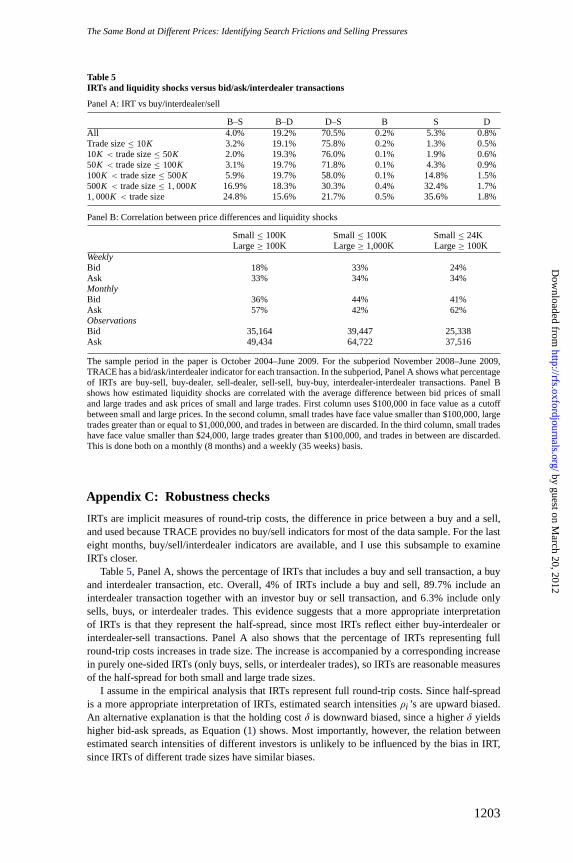
TheSame Bond at Different Prices: Identifying Search Frictions and Selling Pressures
Table 5IRTs and liquidity shocks versus bid/ask/interdealer transactions
Panel A: IRT vs buy/interdealer/sell
B–S B–D D–S B S DAll 4.0% 19.2% 70.5% 0.2% 5.3% 0.8%Trade size≤ 10K 3.2% 19.1% 75.8% 0.2% 1.3% 0.5%10K < tradesize≤ 50K 2.0% 19.3% 76.0% 0.1% 1.9% 0.6%50K < tradesize≤ 100K 3.1% 19.7% 71.8% 0.1% 4.3% 0.9%100K < tradesize≤ 500K 5.9% 19.7% 58.0% 0.1% 14.8% 1.5%500K < tradesize≤ 1,000K 16.9% 18.3% 30.3% 0.4% 32.4% 1.7%1,000K < tradesize 24.8% 15.6% 21.7% 0.5% 35.6% 1.8%
Panel B: Correlation between price differences and liquidityshocks
Small≤ 100K Small≤ 100K Small≤ 24KLarge≥ 100K Large≥ 1,000K Large≥ 100K
WeeklyBid 18% 33% 24%Ask 33% 34% 34%MonthlyBid 36% 44% 41%Ask 57% 42% 62%ObservationsBid 35,164 39,447 25,338Ask 49,434 64,722 37,516
The sample period in the paper is October 2004–June 2009. For the subperiod November 2008–June 2009,TRACE has a bid/ask/interdealer indicator for each transaction. In the subperiod, Panel A shows what percentageof IRTs are buy-sell, buy-dealer, sell-dealer, sell-sell, buy-buy, interdealer-interdealer transactions. Panel Bshows how estimated liquidity shocks are correlated with the average difference between bid prices of smalland large trades and ask prices of small and large trades. First column uses$100,000in face value as a cutoffbetween small and large prices. In the second column, small trades have face value smaller than$100,000,largetrades greater than or equal to$1,000,000,and trades in between are discarded. In the third column, small tradeshave face value smaller than$24,000,large trades greater than$100,000,and trades in between are discarded.This is done both on a monthly (8 months) and a weekly (35 weeks) basis.
Appendix C: Robustness checks
IRTs are implicit measures of round-trip costs, the difference in price between a buy and a sell,and used because TRACE provides no buy/sell indicators for most of the data sample. For the lasteight months, buy/sell/interdealer indicators are available, and I use this subsample to examineIRTs closer.
Table5, Panel A, shows the percentage of IRTs that includes a buy and sell transaction, a buyand interdealer transaction, etc. Overall, 4% of IRTs include a buy and sell, 89.7% include aninterdealer transaction together with an investor buy or sell transaction, and 6.3% include onlysells, buys, or interdealer trades. This evidence suggests that a more appropriate interpretationof IRTs is that they represent the half-spread, since most IRTs reflect either buy-interdealer orinterdealer-sell transactions. Panel A also shows that the percentage of IRTs representing fullround-trip costs increases in trade size. The increase is accompanied by a corresponding increasein purely one-sided IRTs (only buys, sells, or interdealer trades), so IRTs are reasonable measuresof the half-spread for both small and large trade sizes.
I assume in the empirical analysis that IRTs represent full round-trip costs. Since half-spreadis a more appropriate interpretation of IRTs, estimated search intensitiesρi ’s are upward biased.An alternative explanation is that the holding costδ is downward biased, since a higherδ yieldshigher bid-ask spreads, as Equation (1) shows. Most importantly, however, the relation betweenestimated search intensities of different investors is unlikely to be influenced by the bias in IRT,since IRTs of different trade sizes have similar biases.
1203
by guest on March 20, 2012
http://rfs.oxfordjournals.org/D
ownloaded from

TheReview of Financial Studies / v 25 n 4 2012
The identification of liquidity shocks is not affected by the fact that IRTs can be interpretedas a measure of the half-spread. The following example illustrates this. We can find the size of aliquidity shock by looking at, say, the “difference-in-bidprice-differences”γ∗, where
γ∗(s) = [B∗(s)S − B∗(s)L ] − [BS − BL ],
whereS denotes “small trader,” L denotes “large trader,”∗ marks prices under a liquidity shockof size s, and an absence of stars marks prices in equilibrium. Theorem2.3 tells us thatγ∗ isincreasingin s. Assume that we are mistakenly looking at sell transactions for the large trader andbuy for the small trader, so instead ofγ∗ weare investigating
γ∗∗(s) = [B∗(s)S + ωS∗ (s) − B∗(s)L ] − [BS + ωS − BL ]
= [B∗(s)S − B∗(s)L ] − [BS − BL ] + [ωS∗ (s) − ωS],
whereωS is the bid-ask spread for a small trader in equilibrium andωS∗ (s) is the bid-ask spread
under a shock of sizes. According to Theorem2.3,ωS∗ (s) andωS arethe same, soγ∗ = γ∗∗ for
every s. Therefore, liquidity shocks can be identified by looking at eitherγ∗ or γ∗∗. In fact, anycombination of bid, ask, or interdealer prices of small versus large traders can be used to identifyliquidity shocks.
Liquidity shocks can be identified by looking at either bid or ask prices. To test separately on bidand ask prices, I do the following. I sort all bid prices in the period November 2008–June 2009 intosmall and large bid prices. In this robustness check, I use all available straight coupon bullet bondprices with a maturity less than 30 years (I have bid/ask indicators and therefore do not need to filterbid and ask prices out of the data using imputed round-trip trades). For robustness, I use three dif-ferent cutoffs between small and large prices. Trade size of $100,000 to distinguish between insti-tutional and retail investors is one cutoff, prices smaller than $100,000 and larger than $1,000,000is another (throwing in-between prices away), and prices smaller than $24,000 (median trade size)and larger than $100,000 is a third (throwing in-between prices away). For a given bond on a givenday, if I have both a small and a large bid, I have an observation of the difference in bids (if I haveseveral small respectively large bids, I take the average). I average all the differences in bids duringa month to get a monthly average and find the correlation between monthly averages and estimatedmonthly liquidity shocks. I repeat this for ask prices to get a correlation between monthly averageask differences and liquidity shocks. Finally, I repeat this exercise on a weekly basis to provide afurther robustness check. Panel B in Table5 shows the results. Across different specifications,average correlation between estimated liquidity shocks and bid differences is 40%, while thecorresponding average correlation is 52% for ask differences. Thus, differences in prices of smallversus large trades, whether it is bid or ask prices, are correlated with estimated liquidity shocks.
ReferencesAcharya, V., S. Schaefer, and Y. Zhang. 2008. Liquidity Risk and Correlation Risk: A Clinical Study of theGeneral Motors and Ford Downgrade of May 2005. Working Paper, London Business School.
Ambrose, B. W., K. N. Cai, and J. Helwege. 2009. Fallen Angels and Price Pressure. Working Paper.
Ashcraft, A., and D. Duffie. 2007. Systemic Dynamics in the Federal Funds Market.American Economic Review,Papers and Proceedings97:221–25.
Bao, J., J. Pan, and J. Wang. 2011. The Illiquidity of Corporate Bonds.Journal of Finance66:911–46.
Bessembinder, H., K. M. Kahle, W. F. Maxwell, and D. Xu. 2009. Measuring Abnormal Bond Performance.Review of Financial Studies22:4219–58.
Bessembinder, H., and W. Maxwell. 2008. Transparency and the Corporate Bond Market.Journal of EconomicPerspectives22:217–34.
Bessembinder, H., W. Maxwell, and K. Venkaraman. 2006. Market Transparency, Liquidity Externalities, andInstitutional Trading Costs in Corporate Bonds.Journal of Financial Economics82:251–88.
1204
by guest on March 20, 2012
http://rfs.oxfordjournals.org/D
ownloaded from

TheSame Bond at Different Prices: Identifying Search Frictions and Selling Pressures
BIS. 2005. BIS Quarterly Review, June.International Banking and Financial Market Developments1–103.
———. 2008. BIS Quarterly Review, June.International Banking and Financial Market Developments1–93.
Bradley. 1981. Nonparametric Estimates of Standard Error: The Jackknife, the Bootstrap, and Other Methods.Biometrika68:589–99.
Brunnermeier, M. K. 2009. Deciphering the Liquidity and Credit Crunch 2007–08.Journal of EconomicPerspectives23:77–100.
Brunnermeier, M. K., and L. H. Pedersen. 2009. Market Liquidity and Funding Liquidity.Review of FinancialStudies22:2201–38.
Chakravarty, S., and A. Sarkar. 2003. Trading Costs in Three U.S. Bond Markets.Journal of Fixed Income13:39–48.
Chen, L., P. Collin-Dufresne, and R. S. Goldstein. 2009. On the Relation Between the Credit Spread Puzzle andthe Equity Premium Puzzle.Review of Financial Studies22:3367–409.
Chen, Z., A. A. Lookman, N. Schurhoff, and D. Seppi. 2009. Why Ratings Matter: Evidence from Lehman’sIndex Rating Rule Change. Working Paper.
Chen, H., G. Noronha, and V. Singhal. 2004. The Price Response to S&P 500 Index Additions and Deletions:Evidence of Asymmetry and a New Explanation.Journal of Finance59:1901–29.
Coval, J., and E. Stafford. 2007. Asset Fire Sales (and Purchases) in Equity Markets.Journal of FinancialEconomics86:479–512.
Dick-Nielsen, J. 2009. Liquidity Biases in TRACE.Journal of Fixed Income19:43–55.
Dick-Nielsen, J., P. Feldhutter, and D. Lando. Forthcoming. Corporate Bond Liquidity Before and After theOnset of the Subprime Crisis.Journal of Financial Economics.
Duffie, D. 2010. Asset Price Dynamics with Slow-moving Capital.Presidential Address to the American FinanceAssociation.
Duffie, D., N. Garleanu, and L. H. Pedersen. 2005. Over-the-counter Markets.Econometrica73:1815–47.
———. 2007. Valuation in Over-the-counter Markets.Review of Financial Studies20:1865–900.
Edwards, A. K., L. E. Harris, and M. S. Piwowar. 2007. Corporate Bond Market Transaction Cost andTransparency.Journal of Finance62:1421–51.
Ellul, A., C. Jotikasthira, and C. T. Lundblad. 2011 . Regulatory Pressure and Fire Sales in the Corporate BondMarkets.Journal of Financial Economics101:596–620.
Feldhutter, P., and D. Lando. 2008. Decomposing Swap Spreads.Journal of Financial Economics88:375–405.
Fleming, M. J. 2003. Measuring Treasury Market Liquidity.Federal Reserve Bank of New York Economic PolicyReview9:83–108.
Garleanu, N. 2009. Portfolio Choice and Pricing in Illiquid Markets.Journal of Economic Theory144:532–64.
Goldstein, M. A., E. S. Hotchkiss, and E. R. Sirri. 2007. Transparency and Liquidity: A Controlled Experimenton Corporate Bonds.Review of Financial Studies20:235–73.
Green, R., B. Hollifield, and N. Schurhoff. 2007. Financial Intermediation and the Costs of Trading in an OpaqueMarket.Review of Financial Studies20:275–314.
Hong, G., and A. Warga. 2000. An Empirical Study of Bond Market Transactions.Financial Analysts Journal56:32–46.
Huang, J., and M. Huang. 2003. How Much of the Corporate-Treasury Yield Spread Is Due to Credit Risk?Working Paper, Stanford University.
1205
by guest on March 20, 2012
http://rfs.oxfordjournals.org/D
ownloaded from
TheReview of Financial Studies / v 25 n 4 2012
Jarrow, R., H. Li, and F. Zhao. 2007. Interest Rate Caps “Smile” Too! But Can the LIBOR Market ModelsCapture It?Journal of Finance62:345–82.
Kraus, A., and H. R. Stoll. 1972. Price Impacts of Block Trading on the New York Stock Exchange.Journal ofFinance27:569–88.
Kyle, A. 1985. Continuous Auctions and Insider Trading.Econometrica53:1315–35.
Lagos, R., and G. Rocheteau. 2007. Search in Asset Markets: Market Structure, Liquidity, and Welfare.AmericanEconomic Review, Papers and Proceedings97:198–202.
———. 2009. Liquidity in Asset Markets with Search Frictions.Econometrica77:403–26.
Lagos, R., G. Rocheteau, and P.-O. Weill. 2009. Crises and Liquidity in Over-the-counter Markets. WorkingPaper.
Longstaff, F. 2004. The Flight-to-liquidity Premium in U.S. Treasury Bond Prices.Journal of Business77:511–26.
Longstaff, F., S. Mithal, and E. Neis. 2005. Corporate Yield Spreads: Default Risk or Liquidity? New Evidencefrom the Credit-default Swap Market.Journal of Finance60:2213–53.
Merton, R. 1974. On the Pricing of Corporate Debt: The Risk Structure of Interest Rates.Journal of Finance29:449–70.
Mitchell, M., L. H. Pedersen, and T. Pulvino. 2007. Slow-moving Capital.American Economic Review, Papersand Proceedings97:215–20.
Moody’s. 2009. Corporate Default and Recovery Rates, 1920–2008.Moody’s investors Service1–55.
Newman, Y. S., and M. A. Rierson. 2004. Illiquidity Spillovers: Theory and Evidence from European TelecomBond Issuance. Working Paper, Stanford.
Schultz, P. 2001. Bond Trading Costs: A Peak Behind the Curtain.Journal of Finance56:677–98.
1206
by guest on March 20, 2012
http://rfs.oxfordjournals.org/D
ownloaded from