the sami galaxy survey: a new method to estimate molecular

MNRAS 468, 3965–3978 (2017) doi:10.1093/mnras/stx727Advance Access publication 2017 March 27

The SAMI Galaxy Survey: a new method to estimate molecular gassurface densities from star formation rates

Christoph Federrath,1‹ Diane M. Salim,1,2 Anne M. Medling,1,3†Rebecca L. Davies,1,4 Tiantian Yuan,1 Fuyan Bian,1 Brent A. Groves,1 I-Ting Ho,1,5

Robert Sharp,1 Lisa J. Kewley,1 Sarah M. Sweet,1 Samuel N. Richards,2,6,7

Julia J. Bryant,2,6,7 Sarah Brough,6 Scott Croom,2,7 Nicholas Scott,2,7

Jon Lawrence,6 Iraklis Konstantopoulos6 and Michael Goodwin6

1Research School of Astronomy and Astrophysics, Australian National University, Canberra, ACT 2611, Australia2ARC Centre of Excellence for All-sky Astrophysics (CAASTRO), The University of Sydney, NSW 2006, Australia3Cahill Center for Astronomy and Astrophysics, California Institute of Technology, MS 249-17, Pasadena, CA 91125, USA4Max-Planck-Institut fur Extraterrestrische Physik, Giessenbachstrasse, D-85748 Garching, Germany5Institute for Astronomy, University of Hawaii, 2680 Woodlawn Drive, Honolulu, HI 96822, USA6Australian Astronomical Observatory, PO Box 915, North Ryde, NSW 1670, Australia7Sydney Institute for Astronomy, School of Physics, University of Sydney, NSW 2006, Australia

Accepted 2017 March 22. Received 2017 March 19; in original form 2016 October 15

ABSTRACTStars form in cold molecular clouds. However, molecular gas is difficult to observe becausethe most abundant molecule (H2) lacks a permanent dipole moment. Rotational transitions ofCO are often used as a tracer of H2, but CO is much less abundant and the conversion from COintensity to H2 mass is often highly uncertain. Here we present a new method for estimatingthe column density of cold molecular gas (�gas) using optical spectroscopy. We utilize thespatially resolved Hα maps of flux and velocity dispersion from the Sydney-AAO Multi-objectIntegral field spectrograph (SAMI) Galaxy Survey. We derive maps of �gas by inverting themulti-freefall star formation relation, which connects the star formation rate surface density(�SFR) with �gas and the turbulent Mach number (M). Based on the measured range of�SFR = 0.005–1.5 M� yr−1 kpc−2 and M = 18–130, we predict �gas = 7–200 M� pc−2

in the star-forming regions of our sample of 260 SAMI galaxies. These values are closeto previously measured �gas obtained directly with unresolved CO observations of similargalaxies at low redshift. We classify each galaxy in our sample as ‘star-forming’ (219) or‘composite/AGN/shock’ (41), and find that in ‘composite/AGN/shock’ galaxies the average�SFR, M and �gas are enhanced by factors of 2.0, 1.6 and 1.3, respectively, compared tostar-forming galaxies. We compare our predictions of �gas with those obtained by invertingthe Kennicutt–Schmidt relation and find that our new method is a factor of 2 more accurate inpredicting �gas, with an average deviation of 32 per cent from the actual �gas.

Key words: turbulence – techniques: spectroscopic – stars: formation – galaxies: ISM –galaxies: star formation – galaxies: structure.

1 IN T RO D U C T I O N

The coalescence of gases by turbulence and gravity intricately con-trols star formation within giant molecular clouds (Ferriere 2001;

� E-mail: [email protected]†Hubble Fellow.

Elmegreen & Scalo 2004; Mac Low & Klessen 2004; Scalo& Elmegreen 2004; McKee & Ostriker 2007; Hennebelle &Falgarone 2012; Krumholz 2014; Padoan et al. 2014). On onehand, turbulence has the ability to hinder star formation by pro-viding kinetic energy that can oppose gravity. On the other,the supersonic turbulence ubiquitously observed in the molec-ular phase of the interstellar medium (ISM) produces localshocks and compressions, which lead to enhanced gas densities

C© 2017 The AuthorsPublished by Oxford University Press on behalf of the Royal Astronomical Society

Dow

nloaded from https://academ

ic.oup.com/m

nras/article-abstract/468/4/3965/3091133 by University of Q

ueensland Library user on 07 February 2020

mailto:[email protected]

3966 C. Federrath et al.

that are key for triggering star formation (Federrath &Klessen 2012). Understanding the complex effects of turbulence inthe ISM is therefore crucial to understanding the process of galaxyevolution.

The cold turbulent gas that provides the fuel for star forma-tion is only visible in the millimetre/submillimetre to radio wave-lengths, and is often faint, making it difficult to detect at highspatial resolutions. A standard method to measure the mean col-umn density of molecular gas (�gas) is to use rotational lines ofCO. A severe problem with this method is that, because CO isabout 104 times less abundant than the main mass carrier, H2,one requires a CO-to-H2 conversion factor, which is typically cal-ibrated based on measurements in our own Galaxy. However, theCO-to-H2 conversion factor may depend on metallicity, environ-ment and redshift, introducing high uncertainties in the reconstruc-tion of the total gas surface densities from measurements of CO(Shetty et al. 2011a,b). Another method is to measure dust emis-sion or dust extinction and assuming a gas-to-dust ratio to inferthe molecular gas masses and surface densities. These methods cansuffer from uncertainties in the gas-to-dust ratio, especially for low-metallicity galaxies where this ratio becomes increasingly uncer-tain. Both CO and dust observations require telescopes and instru-ments that work at millimetre/submillimetre wavelengths, whichmay not always be available and/or may have relatively low spatialresolution. Here we present a new method to estimate �gas based onthe star formation rate (SFR), which can be obtained with opticalspectroscopy.

Large optical integral field spectroscopy (IFS) surveys havestarted to provide us with details regarding the chemical distri-bution and kinematics of extragalactic sources at a size and uni-formity unprecedented until recent times. Large galaxy surveyssuch as the Sloan Digital Sky Survey (SDSS; York et al. 2000;Abazajian et al. 2009), 2-degree Field Galaxy Redshift Survey(2dFGRS; Colless et al. 2001), the Cosmic Evolution Survey (COS-MOS; Scoville et al. 2007), the VIMOS VLT Deep Survey (VVDS;Le Fevre et al. 2004) and the Galaxy and Mass Assembly survey(GAMA; Driver et al. 2009, 2011) have contributed more than 3.5million spectra that have been of extraordinary aid to our under-standing of galaxy evolution. However, those spectra have beentaken with a single fibre or slit, and provide only a single, globalspectrum per galaxy (Bryant et al. 2015). These spectra are thereforesusceptible to aperture effects because differing parts or fractionsof the galaxies are recorded for each source, thus making each ob-servation dependent on the size and distance of the galaxy, as wellas the positioning of the fibre (Richards et al. 2016). Conversely,IFS can spatially resolve each galaxy observed, thus assigning indi-vidual spectra at many locations across the galaxy. Here we utilizedata from the Sydney-AAO Multi-object Integral field spectrograph(SAMI) Galaxy Survey, an IFS survey with the aim to observe 3400galaxies over a broad range of environments and stellar masses.We use the SFRs measured in SAMI in order to provide a tool forestimating �gas.

The basis of our �gas reconstruction method is a recent star for-mation relation developed in the multi-freefall framework of turbu-lent gas (Hennebelle & Chabrier 2011; Federrath & Klessen 2012;Federrath 2013; Salim, Federrath & Kewley 2015). There havebeen many ongoing efforts to find an intrinsic relation between theamount of gas and the rate at which stars form in a molecular cloud.Initiated by Kennicutt (1998, hereafter K98), �SFR correlates with�gas (Schmidt 1959; K98; Bigiel et al. 2008; Leroy et al. 2008;Daddi et al. 2010; Schruba et al. 2011; Kennicutt & Evans 2012;Renaud, Kraljic & Bournaud 2012), which can be approximated by

an empirical power law with exponent n,

�SFR ∝ �ngas. (1)

For a sample of low-redshift disc and starburst galaxies, K98 foundan exponent of n = 1.40 ± 0.15. However, significant scatter anddiscrepancies between different sets of data exist within this frame-work, commonly referred to as the Kennicutt–Schmidt relation.These discrepancies suggest that �SFR does not only depend on�gas, but also on factors such as the turbulence and the freefall timeof the dense gas on small scales.

Motivated by the fact that dense gas forms stars at a higherrate, a new star formation correlator was derived in Salim et al.(2015, hereafter SFK15). This descriptor, denoted by (�gas/t)multi-ff

and called the ‘maximum or multi-freefall gas consumptionrate’ (MGCR), is dependent on the probability density function(PDF; Vazquez-Semadeni 1994; Padoan, Nordlund & Jones 1997;Passot & Vazquez-Semadeni 1998; Federrath, Klessen &Schmidt 2008) of molecular gas,

�SFR = 0.45 per cent (�gas/t)multi−ff

= 0.45 per cent (�gas/t)single−ff

(1 + b2M2 β

β + 1

)3/8

, (2)

where M is the Mach number of the turbulence, b is the turbulencedriving parameter (Federrath et al. 2008, 2010, 2017) and β is theratio of thermal to magnetic pressure (Padoan & Nordlund 2011;Molina et al. 2012) in the molecular gas.

The SFK15 model for �SFR given by equation (2) is built uponfoundational concepts laid out by Krumholz, Dekel & McKee (2012,hereafter KDM12), which had parametrized �SFR by the ratio be-tween �gas and the average (single) freefall time tff, a correla-tor hereon denoted by (�gas/t)single-ff (KDM12; Federrath 2013;Krumholz 2014). Our new correlator instead uses the concept of amulti-freefall time, which was pioneered by Hennebelle & Chabrier(2011), tested with numerical simulations in Federrath & Klessen(2012), and used in SFK15 as a stepping stone to expand upon theKDM12 model. SFK15 found that �SFR is equal to 0.45 per cent ofthe MGCR by placing observations of Milky Way clouds and theSmall Magellanic Cloud (SMC) in the K98, KDM12 and SFK15frameworks, confirming the measured low efficiency of star for-mation (Krumholz & Tan 2007; Federrath 2015). Statistical testsin SFK15 showed that a significantly better correlation between�SFR and (�gas/t)multi-ff was achieved than that which could be at-tained between either the �gas or (�gas/t)single-ff parametrizations ofthe previous star formation relations by K98 and KDM12, respec-tively. The scatter in the SFK15 relation was found to be a factorof 3–4 lower than in the K98 and KDM12 relations, suggesting thatit provides a better physical model for �SFR compared to the em-pirical relation by K98 and compared to the single-freefall relationby KDM12.

The aim of the current work is to formulate a method to predictthe distribution of �gas by inverting equation (2) and using opticalobservations, which will be plentiful in the coming few years. Herewe use the H α luminosities and velocity dispersions provided bythe SAMI Galaxy Survey to estimate �gas from measurements of�SFR and M.

In Section 2, we describe the observations of our SAMI galaxysample. Section 3 introduces our new method to derive �gas by in-verting the SFK15 relation. In Section 4, we present our results andcompare purely star-forming with composite/AGN/shock galaxiesin our sample. In Section 5, we compare our own and other observa-tions and predictions to previous star formation relations within the

MNRAS 468, 3965–3978 (2017)

Dow


ic.oup.com/m



The SAMI Galaxy Survey: estimating molecular gas 3967

Kennicutt–Schmidt framework. In Section 6, we demonstrate thatour new method for predicting �gas is superior to inverting the K98relation. Our conclusions are summarized in Section 7. The newdata products for each SAMI galaxy in our sample derived here(average turbulent Mach number, cold gas density, freefall time,etc., and finally �gas) are listed in Table A1 in Appendix A and areavailable for download in the online version of the journal or bycontacting the authors.

2 SA M P L E SE L E C T I O N

2.1 The SAMI Galaxy Survey

We selected a sample of 260 galaxies from the SAMI Galaxy Surveyinternal data release version 0.9. The SAMI (Croom et al. 2012)is a front-end fibre feed system for the AAOmega spectrograph(Sharp et al. 2006), consisting of 13 bundles of 61 fibres each(‘hexabundles’; Bland-Hawthorn et al. 2011; Bryant et al. 2014) thatcan be deployed over a 1◦ diameter field of view. SAMI thereforeenables simultaneous spatially resolved spectroscopy of 12 galaxiesand one calibration star with a 15 arcsec diameter field of viewon each object. The AAOmega spectrograph can be configuredto provide different resolutions and wavelength ranges; the SAMIGalaxy Survey employs the 570V grating to obtain a resolution ofR = 1730 (74 km s−1) at 3700–5700 Å and the 1000R grating toobtain R = 4500 (29 km s−1) at 6250–7350 Å. SAMI data cubes arereduced and re-gridded to a spatial scale of 0.5 × 0.5 arcsec2 (Sharpet al. 2015) and the spatial resolution is about 2 arcsec (Green et al.,in preparation).

The SAMI Galaxy Survey plans to include more than 3000 galax-ies at redshift z < 0.1 covering a wide range of stellar masses andenvironments. The sample is drawn from GAMA (Driver et al. 2011)with additional entries from eight nearby clusters to cover denserenvironments (Bryant et al. 2015; Owers et al., in preparation). Re-duced data cubes and a variety of emission-line-based higher leveldata products are included in the first public data release (Allenet al. 2015; Green et al., in preparation).

The emission lines of SAMI galaxies have been analysed usingthe spectral fitting pipeline LZIFU (Ho et al. 2016) to extract emis-sion line fluxes and kinematics for each spectrum. The spectrumassociated with each spectral/spatial pixel (‘spaxel’) is first fit witha stellar template using the ‘penalized pixel-fitting’ (pPXF) routine(Cappellari & Emsellem 2004; Cappellari 2017) before fitting upto three Gaussian line profiles to each of 11 strong emission linessimultaneously. For this paper, we choose to use the single Gaussianfits, and make use of the emission line flux maps, gas velocity mapsand gas velocity dispersion maps below.

Also available in the SAMI Galaxy Survey data base are maps ofSFR and �SFR (in units of M� yr−1 kpc−2). These maps are madeusing extinction-corrected H α fluxes converted to SFRs followingthe relation derived in Kennicutt, Tamblyn & Congdon (1994). TheSFR maps are fully described in Medling et al. (in preparation).

2.2 Our subsample

From the pool of SAMI galaxies, we select a subsample of galaxiesaccording to the criteria described below. We only consider spaxelswith a sufficiently high signal-to-noise ratio (S/N). The S/N was de-fined to be the ratio of the total emission line flux to the statistical 1σ

error in the line flux. This error was inferred using the Levenberg–Marquardt technique of χ2 minimization (Ho et al. 2016). In thefollowing, we list the selection criteria.

(i) Source Extractor (SEXTRACTOR) ellipticity values are available.These values were obtained from the GAMA data base (Driveret al. 2009, 2011; Baldry et al. 2010, 2014; Robotham et al. 2010;Hopkins et al. 2013). We require the ellipticity for each galaxy toestimate the physical volume of gas within each spaxel (explainedin detail in Section 3.3 below).

(ii) The S/N must be ≥5 in the H α, H β, [N II], [S II], [O I] and[O III] emission lines. This allows reliable classification of the emis-sion mechanism. However, in order to measure velocity dispersionsdown to about 12 km s−1, we require and impose an S/N of ≥34in the measured velocity dispersion (explained in detail in Sec-tion 3.1.2 below). We also require that beam smearing (see Sec-tion 3.1.2) did not have a significant effect on the measured velocitydispersion.

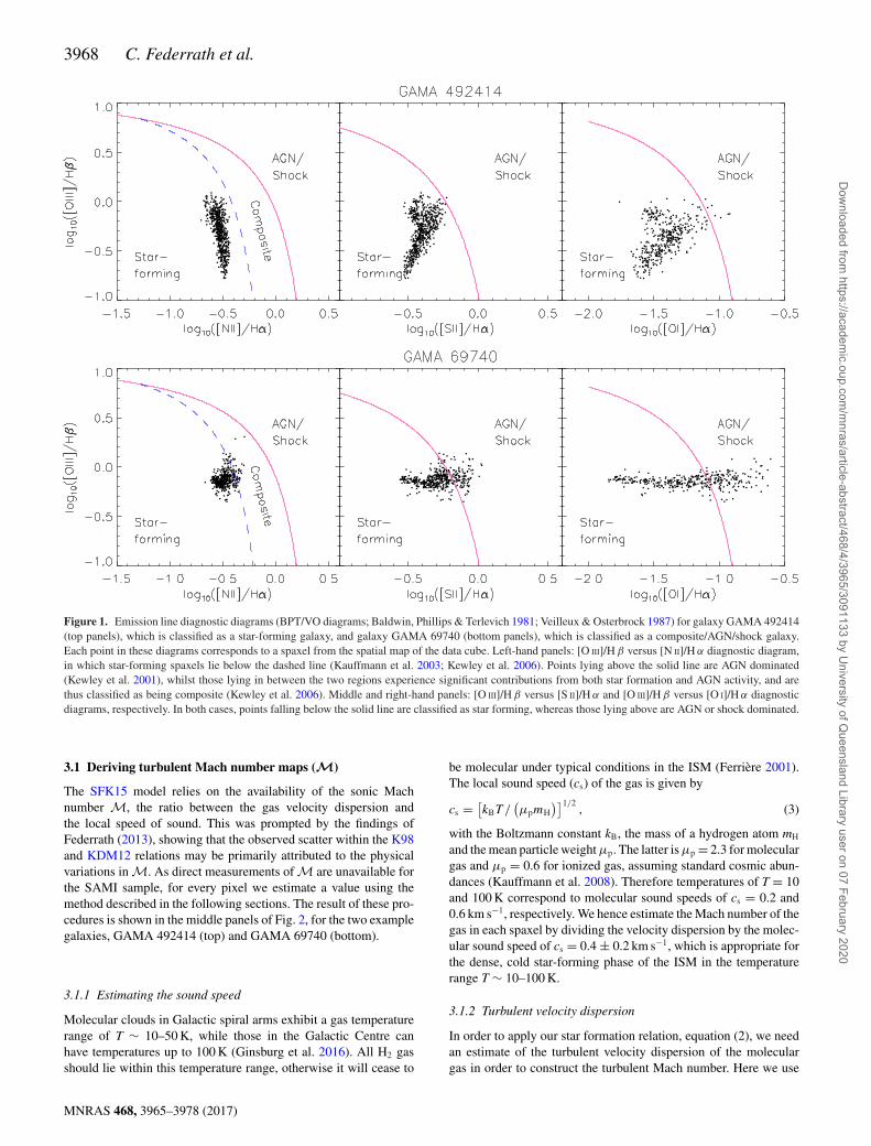
(iii) After removing spaxels that have low S/N and/or are af-fected by beam smearing, the galaxy must have more than 10star-forming spaxels remaining. The star-forming spaxels were fil-tered using the optical classification criteria given in Kewley et al.(2006), an example of which is shown in Fig. 1. This classifica-tion scheme uses optical emission line ratios (BPT/VO diagrams;Baldwin et al. 1981; Veilleux & Osterbrock 1987), in order to distin-guish between star-forming galaxies and galaxies that are dominatedby an active galactic nucleus (AGN) or by shocks. The H α-to-SFRconversion factor used in this work is only valid for star-formingregions, because AGN/shock-dominated spaxels are contaminatedwith emission from AGN/shock regions (Kewley et al. 2002, 2006;Kewley & Dopita 2003; Rich et al. 2010, 2012; Rich, Kewley &Dopita 2011).

Emission line fluxes of each spaxel were corrected for extinctionusing the Balmer decrement and the Cardelli, Clayton & Mathis(1989) reddening curve. Standard extinction for the diffuse ISMwas assumed, with an Rv value of 3.1 being utilized throughout theanalysis (Cardelli et al. 1989; Calzetti et al. 2000).

Each galaxy was classified as either a ‘star-forming’ or ‘compos-ite/AGN/shock’ galaxy. To be classified as star-forming, the galaxyhad to have at least 90 per cent of all valid spaxels lying below andto the left-hand side of the Kauffmann et al. (2003) classificationline in the [O III]/H β versus [N II]/H α diagram, and below and tothe left-hand side of the Kewley et al. (2001) line in the [S II]/H α

and [O I]/H α diagrams, as described in Kewley et al. (2006) (seeFig. 1). A galaxy was classified as composite/AGN/shock, if at least10 per cent of all valid spaxels lie above the Kauffmann et al. (2003)classification line on the [O III]/H β versus [N II]/H α diagram andabove the Kewley et al. (2001) classification line on the [S II]/H α and[O I]/H α diagnostic diagrams. Thus, composite/AGN/shock galax-ies may include composite, AGN or shock (Kewley et al. 2013)galaxies according to the classification in Kewley et al. (2006).These classifications resulted in a sample of 219 star-forming and41 composite/AGN/shock classified galaxies.

3 E S T I M AT I N G T H E M O L E C U L A R G A SSURFAC E D ENSI TY (�gas)

Here we exploit the spatially resolved SAMI H α flux and �SFR

maps in combination with the H α velocity dispersion maps to derivepredictions of �gas across each galaxy in our sample. Examples of�SFR maps are shown in the left-hand panels of Fig. 2 for the star-forming and composite/AGN/shock classified galaxies from Fig. 1.We further derive spaxel-averaged values of the physical parametersfor each galaxy in our subsample.

MNRAS 468, 3965–3978 (2017)

Dow


ic.oup.com/m




Figure 1. Emission line diagnostic diagrams (BPT/VO diagrams; Baldwin, Phillips & Terlevich 1981; Veilleux & Osterbrock 1987) for galaxy GAMA 492414(top panels), which is classified as a star-forming galaxy, and galaxy GAMA 69740 (bottom panels), which is classified as a composite/AGN/shock galaxy.Each point in these diagrams corresponds to a spaxel from the spatial map of the data cube. Left-hand panels: [O III]/H β versus [N II]/H α diagnostic diagram,in which star-forming spaxels lie below the dashed line (Kauffmann et al. 2003; Kewley et al. 2006). Points lying above the solid line are AGN dominated(Kewley et al. 2001), whilst those lying in between the two regions experience significant contributions from both star formation and AGN activity, and arethus classified as being composite (Kewley et al. 2006). Middle and right-hand panels: [O III]/H β versus [S II]/H α and [O III]/H β versus [O I]/H α diagnosticdiagrams, respectively. In both cases, points falling below the solid line are classified as star forming, whereas those lying above are AGN or shock dominated.

3.1 Deriving turbulent Mach number maps (M)

The SFK15 model relies on the availability of the sonic Machnumber M, the ratio between the gas velocity dispersion andthe local speed of sound. This was prompted by the findings ofFederrath (2013), showing that the observed scatter within the K98and KDM12 relations may be primarily attributed to the physicalvariations in M. As direct measurements of M are unavailable forthe SAMI sample, for every pixel we estimate a value using themethod described in the following sections. The result of these pro-cedures is shown in the middle panels of Fig. 2, for the two examplegalaxies, GAMA 492414 (top) and GAMA 69740 (bottom).

3.1.1 Estimating the sound speed

Molecular clouds in Galactic spiral arms exhibit a gas temperaturerange of T ∼ 10–50 K, while those in the Galactic Centre canhave temperatures up to 100 K (Ginsburg et al. 2016). All H2 gasshould lie within this temperature range, otherwise it will cease to

be molecular under typical conditions in the ISM (Ferriere 2001).The local sound speed (cs) of the gas is given by

cs = [kBT /

(μpmH

)]1/2, (3)

with the Boltzmann constant kB, the mass of a hydrogen atom mH

and the mean particle weight μp. The latter is μp = 2.3 for moleculargas and μp = 0.6 for ionized gas, assuming standard cosmic abun-dances (Kauffmann et al. 2008). Therefore temperatures of T = 10and 100 K correspond to molecular sound speeds of cs = 0.2 and0.6 km s−1, respectively. We hence estimate the Mach number of thegas in each spaxel by dividing the velocity dispersion by the molec-ular sound speed of cs = 0.4 ± 0.2 km s−1, which is appropriate forthe dense, cold star-forming phase of the ISM in the temperaturerange T ∼ 10–100 K.

3.1.2 Turbulent velocity dispersion

In order to apply our star formation relation, equation (2), we needan estimate of the turbulent velocity dispersion of the moleculargas in order to construct the turbulent Mach number. Here we use

MNRAS 468, 3965–3978 (2017)

Dow


ic.oup.com/m




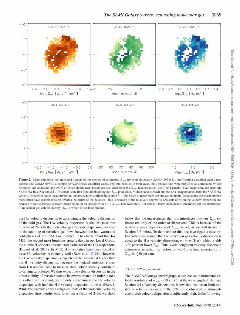
Figure 2. Maps depicting the inputs and outputs of our method of estimating �gas for example galaxy GAMA 492414, a star-forming classified galaxy (toppanels) and GAMA 69740, a composite/AGN/shock classified galaxy (bottom panels). In both cases, only spaxels that were classified as dominated by starformation are analysed, and AGN or shock-dominated spaxels are excluded from the �gas reconstruction. Left-hand panels: �SFR maps obtained from theSAMI H α flux (Section 2.1). This map is the first input to obtaining our �gas prediction. Middle panels: Mach number (M) map obtained from the SAMI H α

velocity dispersion under the assumptions and procedures outlined in Section 3.1. The Mach number maps are our second input. We note that the Mach numbermaps often have spaxels missing towards the centre of the galaxies – this is because of the relatively aggressive S/N cuts of 34 on the velocity dispersion andbecause of our conservative beam smearing cut of all spaxels with σ v < 2 vgrad (see Section 3.1 for details). Right-hand panels: prediction for the distributionof molecular gas column density (�gas), which is our final product.

the H α velocity dispersion to approximate the velocity dispersionof the cold gas. The H α velocity dispersion is similar (to withina factor of 2–3) to the molecular gas velocity dispersion, becauseof the coupling of turbulent gas flows between the hot, warm andcold phases of the ISM. For instance, it has been found that forM33, the second-most luminous spiral galaxy in our Local Group,the atomic H I dispersions are a fair estimator of the CO dispersions(Druard et al. 2014). In M33, H α velocities have been found totrace H I velocities reasonably well (Kam et al. 2015). However,the H α velocity dispersion is expected to be somewhat higher thanthe H2 velocity dispersion, because the ionized emission comesfrom H II regions close to massive stars, which directly contributeto driving turbulence. We thus expect the velocity dispersion in thedirect vicinity of massive stars to be overestimated. In order to takethis effect into account, we crudely approximate the H2 velocitydispersion with half the H α velocity dispersion, σ v = σ v(H α)/2.While this provides only a rough estimate of the molecular velocitydispersion (trustworthy only to within a factor of 2–3), we show

below that the uncertainties that this introduces into our �gas es-timate are only of the order of 50 per cent. This is because of therelatively weak dependence of �gas on M, as we will derive inSection 3.5 below. To demonstrate this, we investigate a case be-low, where we assume that the molecular gas velocity dispersion isequal to the H α velocity dispersion, σ v = σ v(H α), which yields<30 per cent lower �gas. Thus, even though our velocity dispersionestimate is uncertain by factors of ∼2–3, the final uncertainty in�gas is �50 per cent.

3.1.2.1 S/N requirements.

The SAMI/AAOmega spectrograph set-up has an instrumental ve-locity resolution of σ instr = 29 km s−1 at the wavelength of H α (seeSection 2.1). Velocity dispersions below this resolution limit canstill be reliably measured if the S/N in the observed (instrument-convolved) velocity dispersion is sufficiently high. In the following,

MNRAS 468, 3965–3978 (2017)

Dow


ic.oup.com/m




we estimate the required S/N in order to reconstruct intrinsic veloc-ity dispersions down to σ true = 12 km s−1. We choose this cut-off of12 km s−1, because it is the sound speed of the ionized gas, equation(3) with T = 104 K and μp = 0.6, and thus represents a physicallower limit for σ .

The intrinsic (true) velocity dispersion (σ true) can be obtained bysubtracting the instrumental velocity resolution (σ instr) from the ob-served (instrument-convolved) velocity dispersion (σ obs) in quadra-ture, with

σ 2true = σ 2

obs − σ 2instr. (4)

The same relation holds for the uncertainties (noise) in the velocitydispersion,

d(σ 2true) = d(σ 2

obs) − d(σ 2instr),

2σtrued(σtrue) = 2σobsd(σobs) − 2σinstrd(σinstr). (5)

Assuming that the instrumental velocity resolution is fixed, we canuse d(σ instr) = 0 and simplify the last equation to

d(σtrue) = σobs

σtrued(σobs). (6)

Dividing both sides by σ true and substituting equation (4) yields

σobs

d(σobs)= σtrue

d(σtrue)

σ 2obs

σ 2true

= σtrue

d(σtrue)

(1 + σ 2

instr

σ 2true

). (7)

Since (S/N)obs ≡ σ obs/d(σ obs) and (S/N)true ≡ σ true/d(σ true) arethe observed (instrument-convolved) and intrinsic S/N, respec-tively, we can estimate the required (S/N)obs for the target intrinsic(S/N)true = 5 and the target intrinsic velocity dispersion that wewant to resolve, σ true = 12 km s−1, by evaluating

(S/N)obs ≥ (S/N)true

(1 + σ 2

instr

σ 2true

)

≥ 5

[1 +

(29 km s−1

12 km s−1

)2]

= 34. (8)

Thus, for spaxels with observed (instrument-convolved) velocitydispersion S/N greater or equal to 34, we can reliably reconstructthe intrinsic (instrument-corrected) velocity dispersion down to12 km s−1, with an intrinsic S/N of at least 5. We note that theSAMI data base provides the instrument-subtracted velocity dis-persion σ subtracted (VDISP) and its error d(σ subtracted) (VDISP_ERR) basedon the LZIFU fits (Ho et al. 2016). Thus, in order to apply the S/N cutof 34 derived in equation (8), we first reconstruct σobs = (σ 2

subtracted +σ 2

instr)1/2 and its error d(σ obs) = d(σ subtracted)σ subtracted/σ obs, using er-

ror propagation. This criterion is functionally equivalent to settingan S/N cut on the instrument-subtracted velocity dispersion,

(S/N)subtracted = 34

1 + σ 2instr/σ

2subtracted

. (9)

After applying our S/N cuts of 34 to the observed (instrument-convolved) velocity dispersion, any spaxels with velocity disper-sions less than 12 km s−1 are disregarded. We note that this final cutonly removes 1 per cent of the spaxels with (S/N)obs ≥ 34.

3.1.2.2 Beam smearing.

We also have to account for ‘beam smearing’, a phenomenon thatoccurs because of the limitation in spatial resolution of the in-strument. Beam smearing occurs for a physical velocity field thatchanges on spatial scales smaller than the spatial resolution of the

observation. If there is a steep velocity gradient across neighbouringpixels, such as near the centre of a galaxy, beam smearing leads to anartificial increase in the measured velocity dispersion at such spatiallocations. To account for beam smearing, we follow the method inVaridel et al. (2016) and estimate the local velocity gradient vgrad

for a given spaxel with coordinate indices (i, j) as the magnitudeof the vector sum of the difference in the velocities in the adjacentpixels,

vgrad(i, j )

=√

[v(i + 1, j ) − v(i − 1, j )]2+[v(i, j + 1) − v(i, j − 1)]2.

(10)

Note that the differencing to compute vgrad occurs over a linearscale of three SAMI pixels along i and j and thus covers roughlythe spatial resolution of the seeing-limited SAMI observations withfull width at half-maximum (FWHM) ∼ 2 arcsec (see Section 2).If a pixel has a neighbour that is undefined (e.g. because of lowS/N), the gradient in that direction is not taken into account. Asour standard criterion to account for beam smearing, we cut anypixels in which the velocity dispersion is less than twice that of thevelocity gradient (σ v < 2vgrad) and disregard such pixels in furtheranalyses, leaving only spaxels that are largely unaffected by beamsmearing.

In addition to our fiducial beam smearing criterion (σ v < 2vgrad),we test a case with a relaxed beam smearing cut of σ v < vgrad, andfind nearly identical results (see Table 1). We note that our stan-dard beam smearing cut with σ v < 2vgrad tends to remove spaxelsnear the centre of some of the galaxies (see e.g. Fig. 2). However,using the relaxed beam smearing cut with σ v < vgrad yields global(galaxy-averaged) Mach numbers and global �gas estimates thatagree to within 4 per cent with our standard beam smearing cut (seeTable 1), demonstrating that our results are largely unaffected bybeam smearing.

3.1.2.3 Turbulent velocity dispersion versus systematic motions.

Beam smearing is the result of unresolved velocity gradients in theplane-of-the-sky. However, systematic velocity gradients (such asresulting from rotation or large-scale shear) along the line of sight(LOS) also increase the velocity dispersion (even for arbitrarily highspatial resolution) by LOS blending. These large-scale systematicmotions do not represent turbulent gas flows (see e.g. the recentstudy of turbulent motions in the Galactic Centre cloud ‘Brick’,which is subject to large-scale shear; Federrath et al. 2016). As wehave not subtracted or accounted for these factors, our values of theturbulent velocity dispersion may be overestimated.

In summary, we emphasize that the turbulent velocity dispersionhas large uncertainties and is only accurate to within a factor of 2–3.However, the uncertainties that this introduces into our final product(�gas) are �50 per cent, because of the relatively weak dependenceof �gas on M (derived in detail in Section 3.5 below).

3.2 Deriving (�gas/t)multi−ff and (�gas/t)single−ff

To find the MGCR (�gas/t)multi-ff, we divide �SFR (left-hand panelsof Fig. 2) by the SFR efficiency of 0.45 per cent found in SFK15.That is, we invert equation (2),

(�gas/t)multi−ff

[M� yr−1 kpc−2

] = �SFR

0.0045. (11)

MNRAS 468, 3965–3978 (2017)

Dow


ic.oup.com/m




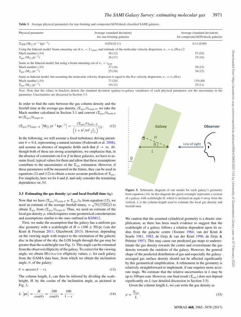
Table 1. Average physical parameters for star-forming and composite/AGN/shock classified SAMI galaxies.

Physical parameter Average (standard deviation) Average (standard deviation)for star-forming galaxies for composite/AGN/shock galaxies

�SFR (M� yr−1 kpc−2) 0.054 (0.11) 0.11 (0.09)

Using the fiducial model: beam smearing cut of σ v < 2 vgrad, and estimate of the molecular velocity dispersion, σ v = σ v(H α)/2Mach number (M) 36 (12) 57 (24)�gas (M� pc−2) 26 (17) 35 (16)

Same as the fiducial model, but using a beam smearing cut of σ v < vgrad

Mach number (M) 37 (14) 59 (23)�gas (M� pc−2) 25 (16) 34 (15)

Same as fiducial model, but assuming the molecular velocity dispersion is equal to the H α velocity dispersion, σ v = σ v(H α)Mach number (M) 71 (24) 110 (48)�gas (M� pc−2) 19 (12) 25 (11)

Note. Note that the values in brackets denote the standard deviation (galaxy-to-galaxy variations) of each physical parameter; not the uncertainty in theparameter. Uncertainties are discussed in Section 3.5.

In order to find the ratio between the gas column density and thefreefall time at the average gas density, (�gas/t)single-ff, we take theMach number calculated in Section 3.1 and convert (�gas/t)multi-ff

to (�gas/t)single-ff,

(�gas/t)single−ff


] = (�gas/t)multi−ff(1 + b2M2 β

β+1

)3/8 . (12)

In the following, we will assume a fixed turbulence driving param-eter b = 0.4, representing a natural mixture (Federrath et al. 2008),and assume an absence of magnetic fields such that β → ∞. Al-though both of these are strong assumptions, we emphasize that, inthe absence of constraints on b or β in these galaxies, we have to as-sume fixed, typical values for them and allow that these assumptionscontribute to the uncertainties of the �gas estimation. However, ifthese parameters will be measured in the future, they can be used inequations (2) and (12) to obtain a more accurate prediction of �gas.For simplicity, here we fix b and β, and only consider the remainingdependence on M.

3.3 Estimating the gas density (ρ) and local freefall time (tff )

Now that we have (�gas/t)single-ff ≡ �gas/tff from equation (12), weneed an estimate of the average freefall timetff = √

3π/(32Gρ) toobtain �gas from (�gas/t)single-ff. Thus, we need an estimate of thelocal gas density ρ, which requires some geometrical considerationsand assumptions similar to the ones outlined in KDM12.

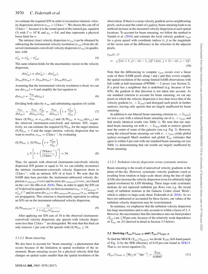
First, we make the assumption that the galaxy has a uniform gasdisc geometry with a scaleheight of H = (100 ± 50) pc (van derKruit & Freeman 2011; Glazebrook 2013). However, dependingon the viewing angle with respect to the orientation of the galacticdisc in the plane of the sky, the LOS length through the gas may begreater than the scaleheight (see Fig. 3). This angle can be estimatedfrom the observed ellipticity of the galaxy. To correct for the viewingangle, we obtain SEXTRACTOR ellipticity values, ε, for each galaxyfrom the GAMA data base, from which we obtain the inclinationangle, θ , of the galaxy:

θ = arccos (1 − ε). (13)

The column length, L, can then be inferred by dividing the scale-height, H, by the cosine of the inclination angle, as pictured inFig. 3,

L[pc

] = H

cos(θ )= 100

cos(θ )= 100

1 − ε. (14)

Figure 3. Schematic diagram of our model for each galaxy’s geometryfrom equation (14). In this diagram the green rectangle represents a sectionof a galaxy with scaleheight H, which is inclined an angle θ away from thevertical. L is the column length used to estimate the local gas density andfreefall time.

We caution that the assumed cylindrical geometry is a drastic sim-plification, as there has been much evidence to suggest that thescaleheight of a galaxy follows a relation dependent upon its ra-dius from the galactic centre (Toomre 1964; van der Kruit &Searle 1981, 1982; de Grijs & van der Kruit 1996; de Grijs &Peletier 1997). This may cause our predicted gas maps to underes-timate the gas density towards the centre and overestimate the gasdensity towards the outskirts of the galaxy. However, the generalshape of the predicted distribution of gas and especially the galaxy-averaged gas surface density should not be affected significantlyby this geometrical simplification. A refinement in the geometry isrelatively straightforward to implement, if one requires more accu-rate maps. We estimate that the relative uncertainties in L may beup to 100 per cent. However, our final result (�gas) does not dependsignificantly on L (see detailed discussion in Section 3.5).

Given the column length L, we can write the gas density as

ρ = �gas

L. (15)

MNRAS 468, 3965–3978 (2017)

Dow


ic.oup.com/m




Since we do not have �gas because it is our final product, we nowsubstitute a rearrangement of the definition of (�gas/t)single-ff,

�gas = (�gas/t)single−ff tff, (16)

as well as the definition of the freefall time in terms of ρ,

tff (ρ) =√

3π

32Gρ, (17)

where G is the gravitational constant. We combine the three previousequations and solve for the gas density,

ρ = (�gas/t)single−ff

L

√3π

32Gρ(18)

⇒ ρ =(√

3π32G

(�gas/t)single−ff

L

)2/3

. (19)

We substitute ρ back into equation (17) to obtain the freefall timetff for the average gas density ρ.

3.4 Deriving our final product, �gas

Finally, we obtain our prediction for �gas either by multiplyingthe freefall time from Section 3.3 by (�gas/t)single-ff calculated inSection 3.2, i.e. using equation (16), or by multiplying the volumedensity ρ from equation (19) by the column length L from equa-tion (14). In terms of the principal observables, �SFR and M =σv/cs, as well as our assumptions for the parameters L = H/(1 − ε),b and β, this corresponds to the final expression for �gas given by

�gas =(

3πL

32G

) 13

⎡⎢⎣ �SFR

0.0045(

1 + b2M2 β

1+β

)3/8

⎤⎥⎦

2/3

. (20)

Two examples of the spatially resolved maps of estimated �gas

based on the new method provided by equation (20) are shown inthe right-hand panels of Fig. 2.

3.5 Uncertainties in the �gas reconstruction

Here we estimate the uncertainties in our �gas prediction based onequation (20). We derive the uncertainties by error propagation ofall variables in equation (20). First, we note that the dependence of�gas on L is weak (�gas ∝ L1/3) and the dependence on M is alsorelatively weak (�gas ∝ M−1/2), which means that the uncertaintiesin L and M enter the final uncertainty in �gas with a weight of 1/3and 1/2, respectively. The strongest dependence of �gas is on theSFR, i.e. �gas ∝ �

2/3SFR, so the uncertainties in �SFR are weighted by

2/3, and we thus expect these to dominate the final uncertainties.Rigorously, the relative uncertainty err(�gas)/�gas from equation(20) is given by

err(�gas)

�gas=

[(1

3

err(L)

L

)2

+(

1

2

err(M)

M)2

+(

2

3

err(�SFR)

�SFR

)2]1/2

, (21)

where we approximated the denominator (1 + b2M2) in equa-tion (20) as b2M2 for the uncertainty propagation (recall that wealso assumed β → ∞), because b2M2 1, based on our velocitydispersion cut and sound speed (see Section 3.1.2). With typicalrelative uncertainties of 70 per cent in L, 100 per cent in M (seeSection 3.1) and 20 per cent in �SFR (based on our S/N cuts of 5

on the H α flux; see Section 2.2), we find a relative uncertaintyof err(�gas)/�gas = 57 per cent, which is dominated by the uncer-tainty in �SFR. Even if the uncertainties in both L and M were 100and 150 per cent, respectively, we would still be able to estimate�gas with an uncertainty of 83 per cent. In summary, despite thelarge uncertainties in M and L (see Sections 3.1 and 3.3), our finaluncertainties in �gas are less than a factor of 2.

4 R ESULTS

4.1 Gas surface density estimates

Our main objective is to estimate �gas from �SFR and the turbulenceproperties (M) in our SAMI galaxy sample. We do this by applyingthe new method introduced in the previous section (Section 3), goingstep-by-step from �SFR to �gas.

Fig. 4 shows each of the �SFR parametrizations explored inSFK15, presented in the same order as the computations of our�gas derivations (Section 3). The framework of the first panel as-sumes a direct correlation between �SFR and (�gas/t)multi-ff. That is,it assumes the star formation relation of equation (2) to hold, thusby construction the SAMI data points in this framework lie alongthe same line. The data points from SFK15 that were used to obtainthis relation are also shown. We note that in the SFK15 derivationof equation (2), the K98 galaxies were omitted because they did nothave (�gas/t)multi-ff values assigned to them due to their lack of Mmeasurements. They are thus similarly excluded in this panel.

Compared to the observational data published in SFK15, weupdated and corrected some of the previous data, and added newobservations in Fig. 4. First, we replace the Bolatto et al. (2011)data for the SMC by the most recent 200 pc resolution data pro-vided in Jameson et al. (2016, J16). We also add the Large Mag-ellanic Cloud (LMC) data from Jameson et al. (2016) and assumethat the SMC and LMC data have Mach numbers in the range10–100, i.e. we basically treat the Mach number as unconstrained,i.e. varying in a plausible range, but we currently do not have directmeasurements of M in the SMC or LMC.1 Second, we replace theglobal central molecular zone (CMZ) data from Yusef-Zadeh et al.(2009) by the local CMZ cloud G0.253+0.016 ‘Brick’ (Federrathet al. 2016; Barnes et al., in preparation) for which significantlymore information is available. We take the values of �gas, M, band β measured in Federrath et al. (2016, F16) and use the SFR perfreefall time estimate of 2 per cent from Barnes et al. (in preparation)to obtain �SFR for the ‘Brick’. The other cloud data are identicalto those published in KDM12, F13 and SFK15, which were takenfrom Heiderman et al. (2010, H10), Gutermuth et al. (2011, G11),Wu et al. (2010, W10) and Lada et al. (2010, L10). However, wecorrected the error bar on the L10 clouds, which showed the stan-dard deviation instead of the standard deviation of the mean inSFK15. We further propagated the uncertainties in �SFR, M andtff between (�gas/t)multi-ff, (�gas/t)single-ff and �gas. Finally, we notethat the observational data included in Fig. 4 cover a wide rangein spatial and spectral resolution (for details we refer the reader tothe source publications of these data), which allowed us to test the

1 The Mach number range of 16–200 assumed in SFK15 for the SMC wassomewhat too high, because the 200 pc resolution data from Bolatto et al.(2011) and Jameson et al. (2016) are more consistent with velocity disper-sions that correspond to M ∼ 10–100 for the SMC and LMC. However,without a direct measurement of the velocity dispersion and gas temperature,the Mach number remains rather unconstrained for the SMC and LMC.

MNRAS 468, 3965–3978 (2017)

Dow


ic.oup.com/m




Figure 4. Left-hand panel: �SFR versus (�gas/t)multi-ff, i.e. the star formation relation derived in SFK15 (equation 2; solid line). The data points shown arethe log-averaged observational data used to derive the SFK15 relation: Heiderman et al. (2010, H10), Gutermuth et al. (2011, G11), Wu et al. (2010, W10) andLada, Lombardi & Alves (2010, L10). Also shown are updated and new observational data based on recent works for the SMC and LMC (Jameson et al. 2016,J16), and for the CMZ cloud ‘Brick’ (Federrath et al. 2016, F16; Barnes et al., in preparation). Error bars are the standard deviation of the mean of the individualcloud data, except for the CMZ cloud ‘Brick’, where the error is taken straight from the measurement. Middle panel: same as left-hand panel, but showing�SFR versus (�gas/t)single-ff (KDM12 relation). We additionally include the individual K98 disc and starburst galaxies tabulated in KDM12 (taking into accountthe corrections by Federrath 2013; Krumholz et al. 2013). Right-hand panel: same as middle panel, but showing �SFR versus �gas, where �gas for the SAMIgalaxies (shown as filled circles in blue for star-forming and orange for composite/AGN/shock) was estimated based on equation (20). Our estimates of �gas

for SAMI lie in close proximity of the low-redshift K98 disc galaxies (filled down-pointing triangles).

universality of the SFK15 relation. In the future, when turbulenceestimates become available for high-redshift data, those need to beincluded as well, to revisit the question of universality of the starformation relation derived in SFK15.

The second panel of Fig. 4 depicts the KDM12 parametrization,�SFR versus (�gas/t)single-ff. The derivation of this value for theSAMI galaxies required inputs from both the H α flux and velocitydispersion, with (�gas/t)single-ff computed from equation (12). Inaddition to the observational data shown in the left-hand panel, weadded the individual K98 disc and starburst galaxies from KDM12(with corrections based on Federrath 2013; Krumholz, Dekel &McKee 2013).

The third panel of Fig. 4 shows the final product of our �gas

predictions; the average gas column density estimate for each of theSAMI galaxies in our sample. These predictions span a range oflog10 �gas [M� pc−2] ∼ 0.9–2.3. We note that the estimated �gas

values for the SAMI galaxies are close to the �gas values of theK98 low-redshift disc galaxies. This is encouraging, because theyare the most similar in type to our sample of SAMI galaxies.The offset in �gas and �SFR by ∼0.5 dex between the SAMI andK98 galaxies can be understood as a consequence of spatial res-olution. In contrast to our spaxel-resolved analysis of the SAMIgalaxies (with spatial resolution of ∼2 arcsec; see Section 2.1),the K98 galaxies are unresolved, which reduces the inferred �SFR

(Federrath & Klessen 2012; Kruijssen & Longmore 2014; Fisheret al. 2017). The reason is that, although the total Hα flux (∝SFR)remains similar even at lower resolutions, the area �A over whichH α is emitted tends to be overestimated and hence the �SFR tendsto be underestimated (�SFR = SFR/�A) for the global K98 data.Similar holds for �gas, because it depends on �A in the same wayas �SFR, and indeed, we find that the resolved SAMI galaxies tendto lie at somewhat higher �gas compared to the unresolved K98 discgalaxy sample.

4.2 Comparison between star-forming andcomposite/AGN/shock galaxies

4.2.1 Gas surface density in star-forming andcomposite/AGN/shock galaxies

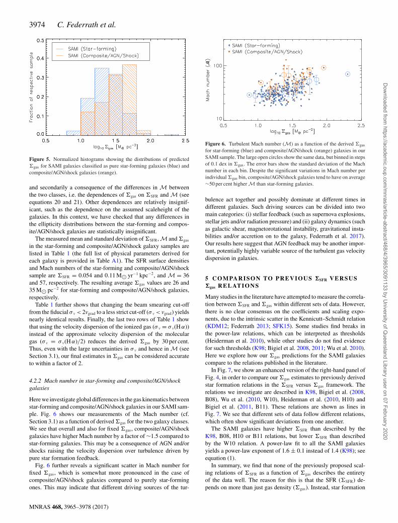
Fig. 4 suggests that the distributions of �gas and �SFR are similarbetween the star-forming and composite/AGN/shock galaxies. Toquantify any statistical differences in �gas between these two sub-samples, we investigate the distribution functions of �gas. Fig. 5shows the histograms of �gas. We see that �gas is enhanced in com-posite/AGN/shock galaxies compared to star-forming galaxies. Thisdifference in �gas between star-forming and composite/AGN/shocktype galaxies is primarily a consequence of the differences in �SFR,

MNRAS 468, 3965–3978 (2017)

Dow


ic.oup.com/m




Figure 5. Normalized histograms showing the distributions of predicted�gas for SAMI galaxies classified as pure star-forming galaxies (blue) andcomposite/AGN/shock galaxies (orange).

and secondarily a consequence of the differences in M betweenthe two classes, i.e. the dependences of �gas on �SFR and M (seeequations 20 and 21). Other dependences are relatively insignif-icant, such as the dependence on the assumed scaleheight of thegalaxies. In this context, we have checked that any differences inthe ellipticity distributions between the star-forming and compos-ite/AGN/shock galaxies are statistically insignificant.

The measured mean and standard deviation of �SFR, M and �gas

in the star-forming and composite/AGN/shock galaxy samples arelisted in Table 1 (the full list of physical parameters derived foreach galaxy is provided in Table A1). The SFR surface densitiesand Mach numbers of the star-forming and composite/AGN/shocksample are �SFR = 0.054 and 0.11 M� yr−1 kpc−2, and M = 36and 57, respectively. The resulting average �gas values are 26 and35 M� pc−2 for star-forming and composite/AGN/shock galaxies,respectively.

Table 1 further shows that changing the beam smearing cut-offfrom the fiducial σ v < 2vgrad to a less strict cut-off (σ v < vgrad) yieldsnearly identical results. Finally, the last two rows of Table 1 showthat using the velocity dispersion of the ionized gas (σ v = σ v(H α))instead of the approximate velocity dispersion of the moleculargas (σ v = σ v(H α)/2) reduces the derived �gas by 30 per cent.Thus, even with the large uncertainties in σ v and hence in M (seeSection 3.1), our final estimates in �gas can be considered accurateto within a factor of 2.

4.2.2 Mach number in star-forming and composite/AGN/shockgalaxies

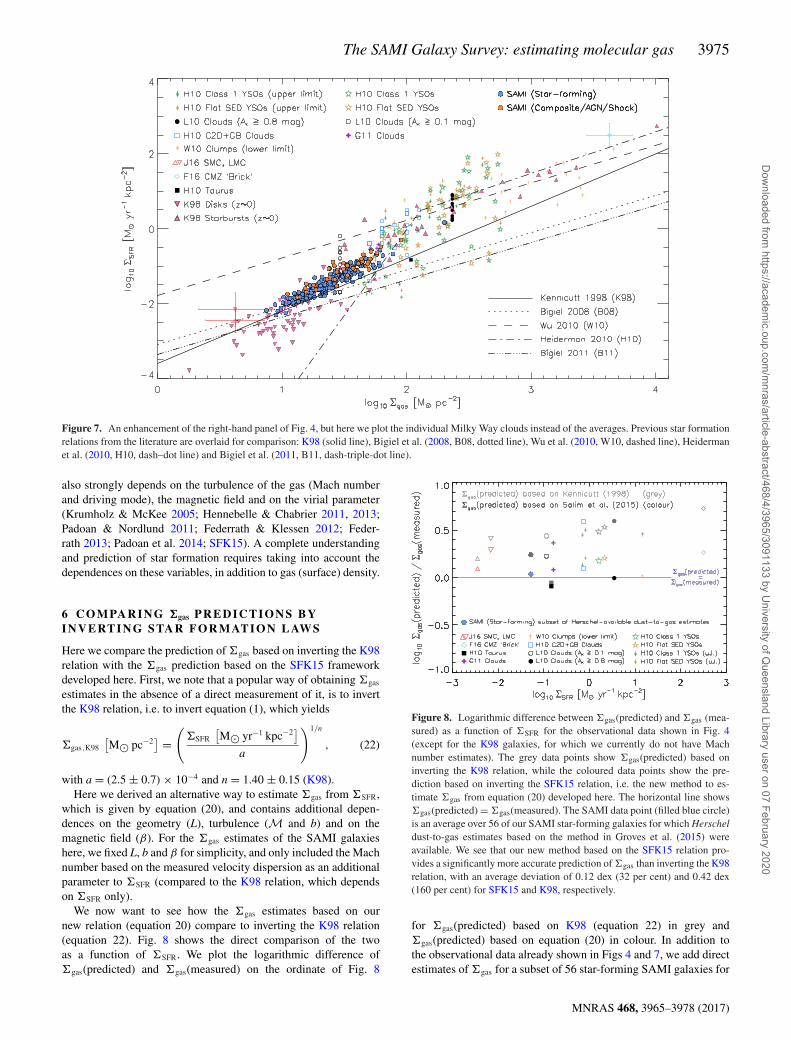
Here we investigate global differences in the gas kinematics betweenstar-forming and composite/AGN/shock galaxies in our SAMI sam-ple. Fig. 6 shows our measurements of the Mach number (cf.Section 3.1) as a function of derived �gas for the two galaxy classes.We see that overall and also for fixed �gas, composite/AGN/shockgalaxies have higher Mach number by a factor of ∼1.5 compared tostar-forming galaxies. This may be a consequence of AGN and/orshocks raising the velocity dispersion over turbulence driven bypure star formation feedback.

Fig. 6 further reveals a significant scatter in Mach number forfixed �gas, which is somewhat more pronounced in the case ofcomposite/AGN/shock galaxies compared to purely star-formingones. This may indicate that different driving sources of the tur-

Figure 6. Turbulent Mach number (M) as a function of the derived �gas

for star-forming (blue) and composite/AGN/shock (orange) galaxies in ourSAMI sample. The large open circles show the same data, but binned in stepsof 0.1 dex in �gas. The error bars show the standard deviation of the Machnumber in each bin. Despite the significant variations in Mach number perindividual �gas bin, composite/AGN/shock galaxies tend to have on average∼50 per cent higher M than star-forming galaxies.

bulence act together and possibly dominate at different times indifferent galaxies. Such driving sources can be divided into twomain categories: (i) stellar feedback (such as supernova explosions,stellar jets and/or radiation pressure) and (ii) galaxy dynamics (suchas galactic shear, magnetorotational instability, gravitational insta-bilities and/or accretion on to the galaxy, Federrath et al. 2017).Our results here suggest that AGN feedback may be another impor-tant, potentially highly variable source of the turbulent gas velocitydispersion in galaxies.

5 C O M PA R I S O N TO PR E V I O U S �SFR V E R S U S�gas R E L AT I O N S

Many studies in the literature have attempted to measure the correla-tion between �SFR and �gas within different sets of data. However,there is no clear consensus on the coefficients and scaling expo-nents, due to the intrinsic scatter in the Kennicutt–Schmidt relation(KDM12; Federrath 2013; SFK15). Some studies find breaks inthe power-law relations, which can be interpreted as thresholds(Heiderman et al. 2010), while other studies do not find evidencefor such thresholds (K98; Bigiel et al. 2008, 2011; Wu et al. 2010).Here we explore how our �gas predictions for the SAMI galaxiescompare to the relations published in the literature.

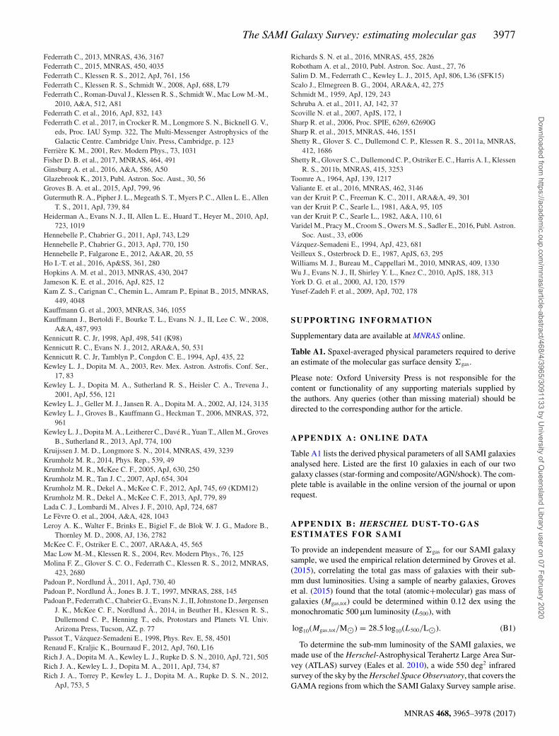
In Fig. 7, we show an enhanced version of the right-hand panel ofFig. 4, in order to compare our �gas estimates to previously derivedstar formation relations in the �SFR versus �gas framework. Therelations we investigate are described in K98, Bigiel et al. (2008,B08), Wu et al. (2010, W10), Heiderman et al. (2010, H10) andBigiel et al. (2011, B11). These relations are shown as lines inFig. 7. We see that different sets of data follow different relations,which often show significant deviations from one another.

The SAMI galaxies have higher �SFR than described by theK98, B08, H10 or B11 relations, but lower �SFR than describedby the W10 relation. A power-law fit to all the SAMI galaxiesyields a power-law exponent of 1.6 ± 0.1 instead of 1.4 (K98); seeequation (1).

In summary, we find that none of the previously proposed scal-ing relations of �SFR as a function of �gas describes the entiretyof the data well. The reason for this is that the SFR (�SFR) de-pends on more than just gas density (�gas). Instead, star formation

MNRAS 468, 3965–3978 (2017)

Dow


ic.oup.com/m




Figure 7. An enhancement of the right-hand panel of Fig. 4, but here we plot the individual Milky Way clouds instead of the averages. Previous star formationrelations from the literature are overlaid for comparison: K98 (solid line), Bigiel et al. (2008, B08, dotted line), Wu et al. (2010, W10, dashed line), Heidermanet al. (2010, H10, dash–dot line) and Bigiel et al. (2011, B11, dash-triple-dot line).

also strongly depends on the turbulence of the gas (Mach numberand driving mode), the magnetic field and on the virial parameter(Krumholz & McKee 2005; Hennebelle & Chabrier 2011, 2013;Padoan & Nordlund 2011; Federrath & Klessen 2012; Feder-rath 2013; Padoan et al. 2014; SFK15). A complete understandingand prediction of star formation requires taking into account thedependences on these variables, in addition to gas (surface) density.

6 C O M PA R I N G �gas P R E D I C T I O N S BYI N V E RTI N G STA R FO R M AT I O N L AW S

Here we compare the prediction of �gas based on inverting the K98relation with the �gas prediction based on the SFK15 frameworkdeveloped here. First, we note that a popular way of obtaining �gas

estimates in the absence of a direct measurement of it, is to invertthe K98 relation, i.e. to invert equation (1), which yields

�gas,K98

[M� pc−2

] =(

�SFR


]a

)1/n

, (22)

with a = (2.5 ± 0.7) × 10−4 and n = 1.40 ± 0.15 (K98).Here we derived an alternative way to estimate �gas from �SFR,

which is given by equation (20), and contains additional depen-dences on the geometry (L), turbulence (M and b) and on themagnetic field (β). For the �gas estimates of the SAMI galaxieshere, we fixed L, b and β for simplicity, and only included the Machnumber based on the measured velocity dispersion as an additionalparameter to �SFR (compared to the K98 relation, which dependson �SFR only).

We now want to see how the �gas estimates based on ournew relation (equation 20) compare to inverting the K98 relation(equation 22). Fig. 8 shows the direct comparison of the twoas a function of �SFR. We plot the logarithmic difference of�gas(predicted) and �gas(measured) on the ordinate of Fig. 8

Figure 8. Logarithmic difference between �gas(predicted) and �gas (mea-sured) as a function of �SFR for the observational data shown in Fig. 4(except for the K98 galaxies, for which we currently do not have Machnumber estimates). The grey data points show �gas(predicted) based oninverting the K98 relation, while the coloured data points show the pre-diction based on inverting the SFK15 relation, i.e. the new method to es-timate �gas from equation (20) developed here. The horizontal line shows�gas(predicted) = �gas(measured). The SAMI data point (filled blue circle)is an average over 56 of our SAMI star-forming galaxies for which Herscheldust-to-gas estimates based on the method in Groves et al. (2015) wereavailable. We see that our new method based on the SFK15 relation pro-vides a significantly more accurate prediction of �gas than inverting the K98relation, with an average deviation of 0.12 dex (32 per cent) and 0.42 dex(160 per cent) for SFK15 and K98, respectively.

for �gas(predicted) based on K98 (equation 22) in grey and�gas(predicted) based on equation (20) in colour. In addition tothe observational data already shown in Figs 4 and 7, we add directestimates of �gas for a subset of 56 star-forming SAMI galaxies for

MNRAS 468, 3965–3978 (2017)

Dow


ic.oup.com/m




which Herschel 500 μm dust measurements were available, usingthe methods in Groves et al. (2015). A detailed description of howthe dust emission was converted to �gas is provided in Appendix B.

In Fig. 8, we see that our new method of estimating �gas from�SFR given by equation (20) is significantly better than simplyinverting the K98 relation, equation (22). We find that our new rela-tion provides �gas estimates with an average deviation of 0.12 dex(32 per cent), while inverting the K98 relation yields an averagedeviation from the true (measured) �gas by 0.42 dex (160 per cent).This shows that our method provides a significantly better �gas pre-diction from �SFR than inverting the K98 relation. Our improved�gas estimate comes at the cost of requiring an estimate of the Machnumber (velocity dispersion) as an additional parameter for the re-construction (prediction) of �gas. However, if �SFR is obtained fromH α (as for the SAMI galaxies analysed here), then we have shownthat the velocity dispersion of H α can be used to estimate the Machnumber (Section 3.1).

Even better �gas predictions based on equation (20) are expectedif the exact scaleheight H, the turbulence driving parameter b andthe magnetic field plasma β are available from future observationsand/or by combining different observational data sets.

7 C O N C L U S I O N S

We presented a new method to estimate the molecular gas columndensity (�gas) of a galaxy using only optical IFS data, by invertingthe star formation relation derived in SFK15. Our method utilizesobserved values of �SFR and velocity dispersion (here from H α) asinputs and returns an estimate of the molecular �gas. The derivationof our method is explained in detail in Section 3, with the final resultgiven by equation (20). We apply our new method to estimate �gas

for star-forming and composite/AGN/shock galaxies classified andobserved in the SAMI Galaxy Survey.

Our main findings from this study are the following.

(i) From the range in �SFR = 0.005–1.5 M� yr−1 kpc−2 andMach number M = 18–130 measured for the SAMI galaxies, wepredict �gas = 7–200 M� pc−2 in the star-forming regions of ourSAMI galaxy sample, consisting of 260 galaxies in total. The pre-dicted values of �gas are similar to those of unresolved low-redshiftdisc galaxies observed in K98. While the K98 galaxies requiredCO detections, here we estimate �gas solely based on H α emissionlines.

(ii) We classify each galaxy in our sample as star-forming or com-posite/AGN/shock. Based on the sample-averaged �SFR = 0.054and 0.11 M� yr−1 kpc−2, and M = 36 and 57 for star-formingand composite/AGN/shock galaxies, respectively, we estimate�gas = 26 and 35 M� pc−2, respectively (see Table 1). We there-fore find that on average, the composite/AGN/shock galaxies haveenhanced �SFR, M and �gas by factors of 2.0, 1.6 and 1.3, respec-tively, compared to the star-forming SAMI galaxies (see Table 1;for each individual SAMI galaxy, see Table A1).

(iii) We discussed methods to account for finite spectral resolu-tion and beam smearing in Section 3.1.2. While the uncertainties arelarge in the velocity dispersion used to estimate the turbulent Machnumber of the molecular gas (Section 3.1), we show that the finalestimate of �gas is accurate to within a factor of 2 (see Section 3.5).

(iv) We compare our new method of estimating �gas from �SFR

with a simple inversion of the K98 relation (Fig. 8). We find thatour new method yields a significantly better estimate of �gas thaninverting the K98 relation, with average deviations from the intrinsic

�gas by 32 per cent for our new method, compared to averagedeviations of 160 per cent from inverting the K98 relation.

AC K N OW L E D G E M E N T S

We thank Mark Krumholz and the anonymous referee for their use-ful comments, which helped to improve this work. CF acknowledgesfunding provided by the Australian Research Council’s (ARC)Discovery Projects (grants DP150104329 and DP170100603).DMS is supported by an Australian Government’s New ColomboPlan scholarship. Support for AMM is provided by NASA throughHubble Fellowship grant #HST-HF2-51377 awarded by the SpaceTelescope Science Institute, which is operated by the Associa-tion of Universities for Research in Astronomy, Inc., for NASA,under contract NAS5-26555. BAG gratefully acknowledges thesupport of the ARC as the recipient of a Future Fellowship(FT140101202). LJK gratefully acknowledges the support of anARC Laureate Fellowship. The SAMI Galaxy Survey is basedon observations made at the Anglo-Australian Telescope. SB ac-knowledges the funding support from the ARC through a FutureFellowship (FT140101166). SC acknowledges the support of anARC Future Fellowship (FT100100457). NS acknowledges sup-port of a University of Sydney Post-doctoral Research Fellowship.The Sydney-AAO Multi-object Integral field spectrograph (SAMI)was developed jointly by the University of Sydney and the Aus-tralian Astronomical Observatory. The SAMI input catalogue isbased on data taken from the Sloan Digital Sky Survey, the GAMASurvey and the VST ATLAS Survey. The SAMI Galaxy Surveyis funded by the ARC Centre of Excellence for All-sky Astro-physics (CAASTRO), through project number CE110001020, andother participating institutions. The SAMI Galaxy Survey websiteis http://sami-survey.org/.

R E F E R E N C E S

Abazajian K. N. et al., 2009, ApJS, 182, 543Allen J. T. et al., 2015, MNRAS, 446, 1567Baldry I. K. et al., 2010, MNRAS, 404, 86Baldry I. K. et al., 2014, MNRAS, 441, 2440Baldwin J. A., Phillips M. M., Terlevich R., 1981, PASP, 93, 5Bigiel F., Leroy A., Walter F., Brinks E., de Blok W. J. G., Madore B.,

Thornley M. D., 2008, AJ, 136, 2846Bigiel F. et al., 2011, ApJ, 730, L13Bland-Hawthorn J. et al., 2011, Opt. Express, 19, 2649Bolatto A. D. et al., 2011, ApJ, 741, 12Bourne N. et al., 2016, MNRAS, 462, 1714Bryant J. J., Bland-Hawthorn J., Fogarty L. M. R., Lawrence J. S., Croom

S. M., 2014, MNRAS, 438, 869Bryant J. J. et al., 2015, MNRAS, 447, 2857Calzetti D., Armus L., Bohlin R. C., Kinney A. L., Koornneef J., Storchi-

Bergmann T., 2000, ApJ, 533, 682Cappellari M., 2017, MNRAS, 466, 798Cappellari M., Emsellem E., 2004, PASP, 116, 138Cardelli J. A., Clayton G. C., Mathis J. S., 1989, ApJ, 345, 245Colless M. et al., 2001, MNRAS, 328, 1039Croom S. M. et al., 2012, MNRAS, 421, 872Daddi E. et al., 2010, ApJ, 714, L118de Grijs R., Peletier R. F., 1997, A&A, 320, L21de Grijs R., van der Kruit P. C., 1996, A&AS, 117, 19Driver S. P. et al., 2009, Astron. Geophys., 50, 12Driver S. P. et al., 2011, MNRAS, 413, 971Druard C. et al., 2014, A&A, 567, A118Eales S. et al., 2010, PASP, 122, 499Elmegreen B. G., Scalo J., 2004, ARA&A, 42, 211

MNRAS 468, 3965–3978 (2017)

Dow


ic.oup.com/m



http://sami-survey.org/


Federrath C., 2013, MNRAS, 436, 3167Federrath C., 2015, MNRAS, 450, 4035Federrath C., Klessen R. S., 2012, ApJ, 761, 156Federrath C., Klessen R. S., Schmidt W., 2008, ApJ, 688, L79Federrath C., Roman-Duval J., Klessen R. S., Schmidt W., Mac Low M.-M.,

2010, A&A, 512, A81Federrath C. et al., 2016, ApJ, 832, 143Federrath C. et al., 2017, in Crocker R. M., Longmore S. N., Bicknell G. V.,

eds, Proc. IAU Symp. 322, The Multi-Messenger Astrophysics of theGalactic Centre. Cambridge Univ. Press, Cambridge, p. 123

Ferriere K. M., 2001, Rev. Modern Phys., 73, 1031Fisher D. B. et al., 2017, MNRAS, 464, 491Ginsburg A. et al., 2016, A&A, 586, A50Glazebrook K., 2013, Publ. Astron. Soc. Aust., 30, 56Groves B. A. et al., 2015, ApJ, 799, 96Gutermuth R. A., Pipher J. L., Megeath S. T., Myers P. C., Allen L. E., Allen

T. S., 2011, ApJ, 739, 84Heiderman A., Evans N. J., II, Allen L. E., Huard T., Heyer M., 2010, ApJ,

723, 1019Hennebelle P., Chabrier G., 2011, ApJ, 743, L29Hennebelle P., Chabrier G., 2013, ApJ, 770, 150Hennebelle P., Falgarone E., 2012, A&AR, 20, 55Ho I.-T. et al., 2016, Ap&SS, 361, 280Hopkins A. M. et al., 2013, MNRAS, 430, 2047Jameson K. E. et al., 2016, ApJ, 825, 12Kam Z. S., Carignan C., Chemin L., Amram P., Epinat B., 2015, MNRAS,

449, 4048Kauffmann G. et al., 2003, MNRAS, 346, 1055Kauffmann J., Bertoldi F., Bourke T. L., Evans N. J., II, Lee C. W., 2008,

A&A, 487, 993Kennicutt R. C. Jr, 1998, ApJ, 498, 541 (K98)Kennicutt R. C., Evans N. J., 2012, ARA&A, 50, 531Kennicutt R. C. Jr, Tamblyn P., Congdon C. E., 1994, ApJ, 435, 22Kewley L. J., Dopita M. A., 2003, Rev. Mex. Astron. Astrofis. Conf. Ser.,

17, 83Kewley L. J., Dopita M. A., Sutherland R. S., Heisler C. A., Trevena J.,

2001, ApJ, 556, 121Kewley L. J., Geller M. J., Jansen R. A., Dopita M. A., 2002, AJ, 124, 3135Kewley L. J., Groves B., Kauffmann G., Heckman T., 2006, MNRAS, 372,

961Kewley L. J., Dopita M. A., Leitherer C., Dave R., Yuan T., Allen M., Groves

B., Sutherland R., 2013, ApJ, 774, 100Kruijssen J. M. D., Longmore S. N., 2014, MNRAS, 439, 3239Krumholz M. R., 2014, Phys. Rep., 539, 49Krumholz M. R., McKee C. F., 2005, ApJ, 630, 250Krumholz M. R., Tan J. C., 2007, ApJ, 654, 304Krumholz M. R., Dekel A., McKee C. F., 2012, ApJ, 745, 69 (KDM12)Krumholz M. R., Dekel A., McKee C. F., 2013, ApJ, 779, 89Lada C. J., Lombardi M., Alves J. F., 2010, ApJ, 724, 687Le Fevre O. et al., 2004, A&A, 428, 1043Leroy A. K., Walter F., Brinks E., Bigiel F., de Blok W. J. G., Madore B.,

Thornley M. D., 2008, AJ, 136, 2782McKee C. F., Ostriker E. C., 2007, ARA&A, 45, 565Mac Low M.-M., Klessen R. S., 2004, Rev. Modern Phys., 76, 125Molina F. Z., Glover S. C. O., Federrath C., Klessen R. S., 2012, MNRAS,

423, 2680Padoan P., Nordlund Å., 2011, ApJ, 730, 40Padoan P., Nordlund Å., Jones B. J. T., 1997, MNRAS, 288, 145Padoan P., Federrath C., Chabrier G., Evans N. J., II, Johnstone D., Jørgensen

J. K., McKee C. F., Nordlund Å., 2014, in Beuther H., Klessen R. S.,Dullemond C. P., Henning T., eds, Protostars and Planets VI. Univ.Arizona Press, Tucson, AZ, p. 77

Passot T., Vazquez-Semadeni E., 1998, Phys. Rev. E, 58, 4501Renaud F., Kraljic K., Bournaud F., 2012, ApJ, 760, L16Rich J. A., Dopita M. A., Kewley L. J., Rupke D. S. N., 2010, ApJ, 721, 505Rich J. A., Kewley L. J., Dopita M. A., 2011, ApJ, 734, 87Rich J. A., Torrey P., Kewley L. J., Dopita M. A., Rupke D. S. N., 2012,

ApJ, 753, 5

Richards S. N. et al., 2016, MNRAS, 455, 2826Robotham A. et al., 2010, Publ. Astron. Soc. Aust., 27, 76Salim D. M., Federrath C., Kewley L. J., 2015, ApJ, 806, L36 (SFK15)Scalo J., Elmegreen B. G., 2004, ARA&A, 42, 275Schmidt M., 1959, ApJ, 129, 243Schruba A. et al., 2011, AJ, 142, 37Scoville N. et al., 2007, ApJS, 172, 1Sharp R. et al., 2006, Proc. SPIE, 6269, 62690GSharp R. et al., 2015, MNRAS, 446, 1551Shetty R., Glover S. C., Dullemond C. P., Klessen R. S., 2011a, MNRAS,

412, 1686Shetty R., Glover S. C., Dullemond C. P., Ostriker E. C., Harris A. I., Klessen

R. S., 2011b, MNRAS, 415, 3253Toomre A., 1964, ApJ, 139, 1217Valiante E. et al., 2016, MNRAS, 462, 3146van der Kruit P. C., Freeman K. C., 2011, ARA&A, 49, 301van der Kruit P. C., Searle L., 1981, A&A, 95, 105van der Kruit P. C., Searle L., 1982, A&A, 110, 61Varidel M., Pracy M., Croom S., Owers M. S., Sadler E., 2016, Publ. Astron.

Soc. Aust., 33, e006Vazquez-Semadeni E., 1994, ApJ, 423, 681Veilleux S., Osterbrock D. E., 1987, ApJS, 63, 295Williams M. J., Bureau M., Cappellari M., 2010, MNRAS, 409, 1330Wu J., Evans N. J., II, Shirley Y. L., Knez C., 2010, ApJS, 188, 313York D. G. et al., 2000, AJ, 120, 1579Yusef-Zadeh F. et al., 2009, ApJ, 702, 178

S U P P O RT I N G IN F O R M AT I O N

Supplementary data are available at MNRAS online.

Table A1. Spaxel-averaged physical parameters required to derivean estimate of the molecular gas surface density �gas.

Please note: Oxford University Press is not responsible for thecontent or functionality of any supporting materials supplied bythe authors. Any queries (other than missing material) should bedirected to the corresponding author for the article.

APPENDI X A : O NLI NE DATA

Table A1 lists the derived physical parameters of all SAMI galaxiesanalysed here. Listed are the first 10 galaxies in each of our twogalaxy classes (star-forming and composite/AGN/shock). The com-plete table is available in the online version of the journal or uponrequest.

APPENDI X B: HERSCHEL D U S T-TO - G A SESTI MATES FOR SAMI

To provide an independent measure of �gas for our SAMI galaxysample, we used the empirical relation determined by Groves et al.(2015), correlating the total gas mass of galaxies with their sub-mm dust luminosities. Using a sample of nearby galaxies, Groveset al. (2015) found that the total (atomic+molecular) gas mass ofgalaxies (Mgas,tot) could be determined within 0.12 dex using themonochromatic 500 μm luminosity (L500), with

log10(Mgas,tot/M�) = 28.5 log10(L500/L�). (B1)

To determine the sub-mm luminosity of the SAMI galaxies, wemade use of the Herschel-Astrophysical Terahertz Large Area Sur-vey (ATLAS) survey (Eales et al. 2010), a wide 550 deg2 infraredsurvey of the sky by the Herschel Space Observatory, that covers theGAMA regions from which the SAMI Galaxy Survey sample arise.

MNRAS 468, 3965–3978 (2017)

Dow


ic.oup.com/m



https://academic.oup.com/mnras


Table A1. Spaxel-averaged physical parameters required to derive an estimate of the molecular gas surface density �gas. Here only the first 10 galaxies ineach of our two samples classified as star-forming or composite/AGN/shock are shown. The complete table is available in the online version of the journal.

GAMA Redshift ε Nspax Lspax �SFR M ρ tff (�gas/t)multi-ff (�gas/t)single-ff �gas

ID (pc) (M� yr−1 kpc−2) (10−24 g cm−3) (Myr) (M� yr−1 kpc−2) (M� yr−1 kpc−2) (M� pc−2)

Star-forming classified galaxies

8353 0.020 0.30 361 200 0.036 ± 0.007 28 ± 19 12 ± 6 19 ± 5 7.9 ± 1.6 1.3 ± 0.7 25 ± 168570 0.021 0.65 10 210 0.0057 ± 0.0011 21 ± 15 2.5 ± 1.3 42 ± 11 1.3 ± 0.3 0.25 ± 0.14 11 ± 79352 0.024 0.17 40 250 0.065 ± 0.013 32 ± 23 18 ± 9 16 ± 4 14 ± 3 2.1 ± 1.2 33 ± 2015218 0.026 0.69 29 260 0.0062 ± 0.0012 34 ± 24 1.9 ± 1.0 48 ± 12 1.4 ± 0.3 0.19 ± 0.11 9.2 ± 5.716026 0.054 0.49 36 520 0.10 ± 0.02 77 ± 54 12 ± 6 19 ± 5 23 ± 5 1.7 ± 1.0 34 ± 2116294 0.029 0.30 11 290 0.010 ± 0.002 23 ± 16 5.6 ± 2.8 28 ± 7 2.2 ± 0.4 0.43 ± 0.24 12 ± 722633 0.070 0.17 289 660 0.065 ± 0.013 35 ± 25 18 ± 9 16 ± 4 14 ± 3 2.0 ± 1.1 31 ± 1922839 0.039 0.29 17 390 0.010 ± 0.002 30 ± 21 4.9 ± 2.5 30 ± 8 2.2 ± 0.4 0.34 ± 0.19 10 ± 622932 0.039 0.29 94 390 0.013 ± 0.003 25 ± 18 6.5 ± 3.3 26 ± 7 2.9 ± 0.6 0.52 ± 0.29 14 ± 823591 0.025 0.15 17 260 0.078 ± 0.016 36 ± 25 20 ± 10 15 ± 4 17 ± 3 2.3 ± 1.3 35 ± 21... ... ... ... ... ... ... ... ... ... ... ...

Composite/AGN/shock classified galaxies

69740 0.013 0.45 221 140 0.13 ± 0.03 63 ± 45 15 ± 8 17 ± 4 28 ± 6 2.4 ± 1.4 41 ± 2678531 0.055 0.23 12 530 0.12 ± 0.02 86 ± 61 16 ± 8 17 ± 4 27 ± 5 1.9 ± 1.1 31 ± 1985416 0.019 0.51 91 200 0.16 ± 0.03 61 ± 43 17 ± 8 16 ± 4 34 ± 7 3.1 ± 1.8 51 ± 3199349 0.020 0.63 104 200 0.081 ± 0.016 32 ± 23 12 ± 6 19 ± 5 18 ± 4 2.6 ± 1.5 50 ± 31106376 0.040 0.21 211 400 0.10 ± 0.02 29 ± 20 25 ± 13 13 ± 3 22 ± 4 3.5 ± 2.0 47 ± 29106389 0.040 0.59 21 400 0.080 ± 0.016 49 ± 35 11 ± 5 20 ± 5 18 ± 4 1.9 ± 1.1 38 ± 24144239 0.018 0.54 204 190 0.044 ± 0.009 43 ± 31 8.2 ± 4.1 23 ± 6 9.7 ± 1.9 1.1 ± 0.6 26 ± 16144320 0.052 0.23 40 500 0.079 ± 0.016 61 ± 43 14 ± 7 18 ± 4 17 ± 3 1.6 ± 0.9 28 ± 17204799 0.017 0.40 59 180 0.23 ± 0.05 69 ± 48 23 ± 12 14 ± 3 50 ± 10 4.2 ± 2.4 58 ± 36210660 0.017 0.48 59 170 0.029 ± 0.006 22 ± 15 9.6 ± 4.9 21 ± 5 6.5 ± 1.3 1.3 ± 0.7 27 ± 17... ... ... ... ... ... ... ... ... ... ... ...

Note. All galaxy parameters are based on a straight average over all valid spaxels and the uncertainties were propagated based on the average values.Column 1: GAMA ID. Column 2: redshift. Column 3: ellipticity. Column 4: number of valid spaxels for gas column density estimate. Column 5: linear size ofeach spaxel. Column 6: spaxel-averaged �SFR. Column 7: spaxel-averaged turbulent Mach number. Column 8: spaxel-averaged gas volume density, estimatedbased on equation (19). Column 9: spaxel-averaged freefall time based on equation (17). Column 10: spaxel-averaged multi-freefall gas consumption rate,(�gas/t)multi-ff; equation (11). Column 11: spaxel-averaged single-freefall gas consumption rate, (�gas/t)single-ff; equation (12). Column 12: spaxel-averagedmolecular gas surface density �gas, estimated with equation (20).

In particular, we cross-matched the 219 star-forming SAMI galax-ies classified here against the single-entry source catalogue fromHerschel-ATLAS Data Release 1 (Bourne et al. 2016; Valianteet al. 2016).2 Of the 219 SAMI star-forming galaxies, 128 haveHerschel detections. Of these, 56 have significant detections (S/N> 3) in the Spectral and Photometric Imaging Receiver (SPIRE)500 μm band.

To convert the total gas mass to a gas surface density we requireda surface area over which the infrared flux is emitted. Given the largebeam size of the SPIRE 500 μm observations, the SAMI galaxiesare unresolved. However, as can be seen in the radial profiles of thenearby galaxy sample used in Groves et al. (2015, in particular theirfig. 7 and online figures), the highest surface brightness regionsoccur within half an optical radius (∼0.5R25 or 1.8Re based onWilliams, Bureau & Cappellari 2010), with most of the infraredluminosity (and molecular gas mass) occurring within this radius.Groves et al. (2015) further find that at this radius, the atomic and

2 Available at http://www.h-atlas.org/public-data/download

molecular gas surface densities are about the same (the ratio of thetotal atomic and molecular gas masses inside 0.5R25 is also aboutunity). Based on those findings, we approximated the moleculargas mass within 0.5R25 with 0.5Mgas, tot. Therefore, we derive themolecular �gas through

�gas = 0.5Mgas,tot

π (1.8Re)2 (1 − ε), (B2)

where the effective radius Re and ellipticity ε of the SAMI galaxiesare as derived in the GAMA survey (Driver et al. 2011).

This paper has been typeset from a TEX/LATEX file prepared by the author.

MNRAS 468, 3965–3978 (2017)

Dow


ic.oup.com/m



http://www.h-atlas.org/public-data/download

the sami galaxy survey: a new method to estimate molecular

Documents