The Search and Matching Model: Challenges

and Solutions

Demetris Koursaros

Submitted in partial fulfillment of the

requirements for the degree of

Doctor of Philosophy

in the Graduate School of Arts and Sciences

COLUMBIA UNIVERSITY

2011

© 2011

Demetris Koursaros

All rights reserved

The Search and Matching Model: Challenges and

Solutions

Demetris Koursaros

Abstract

This dissertation focuses on explaining the cyclicality of unemployment, job vacancies, job

creation and market tightness in the US economy. The framework used to model unemployment

and job creation throughout this work, is the search and matching model, created by Mortensen

and Pissarides (1994). This dissertation proposes three different mechanisms to improve the

performance of a dynamic stochastic general equilibrium model (DSGE) with search

unemployment, to align the model’s predictions with the quarterly US data from 1955-2005.

The first chapter proposes a New Keynesian model with search and matching frictions in the

labor market that can account for the cyclicality and persistence of vacancies, unemployment,

job creation, inflation and the real wage, after a monetary shock. Motivated by evidence from

psychology, unemployment is modeled as a social norm. The norm is the belief that individuals

should exert effort to earn their living and free riders are a burden to society. Households

pressure the unemployed to find jobs: the less unemployed workers there are, the more

supporters the norm has and therefore the greater the pressure and psychological cost

experienced by each unemployed searcher. By altering the value of being unemployed, this

procyclical psychological cost hinders the wage from crowding out vacancy creation after a

monetary shock. Thus, the model is able to capture the high volatility of vacancies and

unemployment observed in the data, accounting for the Shimer puzzle. The paper also departs

from the literature by introducing price rigidity in the labor market, inducing additional inertia

and persistence in the response of inflation and the real wage after a monetary shock. The

model's responses after a monetary shock are in line with the responses obtained from a VAR on

US data.

In the second chapter I attempt to solve the amplification puzzle, the inability of the standard

search and matching model to account for the volatility in vacancies and unemployment, by

exploring the connection between R&D and employment. R&D affects product creation and

product creation affects employment. An improvement in technology benefits the economy in

two ways. Same products can be produced more efficiently and also new products are created.

Empirical evidence suggests that the increase in production for already existing goods does not

imply increases in employment, while new products are associated with increases in employment.

The search and matching model implies that changes in technology do not imply large changes

in employment for already existing goods which is in line with what the evidence suggest.

However, when the search and matching model applies for sectors that innovate and produce

new products, changes in employment significantly increase. Therefore, in this model I assume

all agents need to innovate first before they create a job opening, because firms that invent new

products are the ones that contribute more to the volatility of employment according to the

evidence. Since ideas are cheaper to implement after a technological expansion, the cost of

vacancies becomes countercyclical which boosts job creation and vacancies. The model can

amplify the volatilities of vacancies, unemployment and market tightness approximately by up to

300 percent.

The third chapter investigates the macroeconomic implications from introducing perpetual

learning in a simple search and matching model. When the agents with rational expectations are

replaced with agents that are boundedly rational, the volatilities of vacancies, unemployment and

market tightness are increased significantly. Job creation is connected to the present discounted

value of future cash flows, which means that if agents do not form rational expectations, their

forecasts of future cash flows are subject to periods of either excess optimism or excess

pessimism. Those extra distortions of the agents' forecasts amplify the volatility of job creation.

Therefore, the amplification puzzle arising from the search and matching model might be due to

the strong assumption that agents are rational; thus, when agents need to form multi-period

forecasts using past data as in Preston (2005) and Eusepi and Preston (2010), the search and

matching model's amplification potential is enhanced. The model can replicate moments from

quarterly US data from 1955Q1 to 2007Q4. However the more amplification added to the model

through higher gain parameter, the further the correlations generated by the model are from the

ones obtained from US data. That is because higher amplification induces vacancies to fluctuate

around the rational expectations equilibrium less smoothly. Moreover, higher amplification

through learning worsens the prediction of the model for the slope of the Beveridge curve.

i

Contents: Chapter 1 - Labor market dynamics when (un)employment is a

social norm

1. Introduction .......................................................................................................................... 2

2. The puzzles and the social norm mechanism ........................................................................... 5

2.1 The amplification puzzle..................................................................................................... 6

2.2 Social norms and the norm of unemployment .................................................................... 7

2.3 Defining unemployment as a social norm ........................................................................ 10

2.4 A job market framework and unemployment as a social norm ........................................ 12

2.5 Unemployment as a social norm and the amplification puzzle......................................... 14

3. The Model ..................................................................................................................................... 15

3.1 The agents ......................................................................................................................... 15

3.2 Households........................................................................................................................ 16

3.2.1 Household Problem ................................................................................................. 19

3.3 Intermediate firms ............................................................................................................. 20

3.3.1 The value of job and unemployment ....................................................................... 21

3.3.2 The value of a job to the firm .................................................................................. 22

3.3.3 The value of employment and unemployment ........................................................ 22

3.3.4 The job creation condition ...................................................................................... 23

3.3.5 The bargaining process ........................................................................................... 24

3.3.6 The wage equation .................................................................................................. 16

3.4 Retail firms ....................................................................................................................... 28

3.5 Government and Monetary authority ................................................................................ 30

3.5.1 Government ............................................................................................................. 30

3.5.2 Monetary authority .................................................................................................. 30

3.6 Equilibrium ......................................................................................................................... 9

4. Calibration, estimation and results ............................................................................................ 33

4.1 Calibration .................................................................................................................. 33

4.2 The estimation procedure ........................................................................................... 34

4.3 The estimates .............................................................................................................. 35

4.4 The model’s ability to match the data ........................................................................ 37

4.5 The main ingredients .................................................................................................. 37

ii

4.5.1 The introduction of unemployment as a social norm .............................................. 37

4.5.2 The introduction of price stickiness in the intermediate sector............................... 39

4.5.3 Other ingredients ..................................................................................................... 42

5. Conclusion .................................................................................................................................... 43

6. Bibliography ................................................................................................................................. 44

7. Appendix A ................................................................................................................................... 49

8. Appendix B ................................................................................................................................... 52

9. Appendix C ................................................................................................................................... 54

10. Appendix D ................................................................................................................................... 57

11. Appendix E ................................................................................................................................... 60

12. Appendix F ................................................................................................................................... 63

13. Appendix G ................................................................................................................................... 64

Contents: Chapter 2 - R&D, Product Innovation and Employment

1. Introduction ........................................................................................................................ 71

2. The impact of R&D on employment ...................................................................................... 73

3. R&D firms ............................................................................................................................ 76

2.1 The vacancy cost ............................................................................................................... 78

2.2 Puzzle and solution ........................................................................................................... 79

4. The Model ..................................................................................................................................... 82

4.1 Household problem ........................................................................................................... 82

4.2 The Bellman equations ..................................................................................................... 84

4.2.1 The firms ................................................................................................................. 84

4.2.2 The workers............................................................................................................. 85

4.2.3 Bargaining and wage ............................................................................................... 85

4.2.4 The solution............................................................................................................. 89

4.2.5 The price of ideas and vacancy dynamics ............................................................... 90

5. Calibration, estimation and results ............................................................................................ 91

5.1 Calibration .................................................................................................................. 92

5.2 Result .......................................................................................................................... 93

6. Conclusion .................................................................................................................................... 94

7. Bibliography ................................................................................................................................. 95

iii

Contents: Chapter 3 - The Search and Matching Model when Agents are

Learning

1. Introduction ...................................................................................................................... 101

2. The model ......................................................................................................................... 104

2.1 Households...................................................................................................................... 105

2.1.1 The households problem ....................................................................................... 106

2.1.2 The Bellman equations .......................................................................................... 108

2.2 Firms ............................................................................................................................... 109

2.2.1 Nash bargaining .................................................................................................... 112

2.3 Household problem revisited .......................................................................................... 113

2.3.1 The intertemporal budget constraint ..................................................................... 114

2.3.2 The consumption equation .................................................................................... 116

2.4 Equilibrium and aggregate dynamics .............................................................................. 116

2.5 Expectations .................................................................................................................... 118

2.5.1 Timing ................................................................................................................... 119

2.5.2 Perpetual learning ................................................................................................. 120

2.6 The solution .................................................................................................................... 121

3. Simulation and results ............................................................................................................... 123

3.1 Calibration ................................................................................................................ 123

3.2 Data .......................................................................................................................... 124

3.3 Results ...................................................................................................................... 125

3.4 Alternative model specification ................................................................................ 131

3.5 The distribution of beliefs ........................................................................................ 133

4. Conclusion .................................................................................................................................. 134

5. Bibliography ............................................................................................................................... 135

6. Appendix A ................................................................................................................................. 137

7. Appendix B ................................................................................................................................. 138

8. Appendix C ................................................................................................................................. 139

9. Appendix D ................................................................................................................................. 141

10. Appendix E ................................................................................................................................. 145

11. Appendix F ................................................................................................................................. 147

List of Figures & Tables: Chapter 1 1. Figure 1: Empirical impulse responses .................................................................................... 6

iv

2. Figure 2: Evidence from Clark (2003) ....................................................................................... 9

3. Figure 3: Model outline ........................................................................................................ 17

4. Figure 4: Main Result ........................................................................................................... 65

5. Figure 5: Result without social norm ..................................................................................... 66

6. Figure 6: The effect of the social norm .................................................................................. 66

7. Figure 7: Get rid of the job market specification .................................................................... 67

8. Figure 8: Result without the job market ................................................................................ 67

9. Figure 9: Impulse responses with flexible prices .................................................................... 68

10. Figure 10: Impulse responses and flexible prices in the intermediate sector .......................... 69

11. Figure 11: Responses without vacancy adjustment costs ....................................................... 69

12. Table 1: The calibration ........................................................................................................ 35

13. Table 2: The estimated parameters ...................................................................................... 36

List of Figures & Tables: Chapter 2 1. Figure 1: Model outline ........................................................................................................ 81

2. Figure 2: Impulse responses of vacancies .............................................................................. 98

3. Figure 3: Impulse responses of unemployment .................................................................... 98

4. Figure 4: Impulse responses of market tightness ................................................................... 99

5. Table 1: The calibration ........................................................................................................ 92

6. Table 2: The table of second moments .................................................................................. 93

List of Figures & Tables: Chapter 3 1. Figure 1: Impulse responses with gain 0.0055 ..................................................................... 156

2. Figure 2: Impulse responses with gain 0.006 ....................................................................... 157

3. Figure 3: Responses of vacancies ........................................................................................ 158

4. Figure 4: Convergence of the belief parameters with decreasing gain .................................. 160

5. Figure 5: The distribution of beliefs .................................................................................... 161

6. Table 1: The calibration ...................................................................................................... 124

7. Table 2: US data moments.................................................................................................. 153

8. Table 3: RE moments ......................................................................................................... 153

v

9. Table 4: Moments with gain 0.0045 .................................................................................... 153

10. Table 5: Moments with gain 0.005 ...................................................................................... 154

11. Table 6: Moments with gain 0.0055 .................................................................................... 154

12. Table 7: Amplification ........................................................................................................ 154

13. Table 8: Autocorrelations ................................................................................................... 155

14. Table 9: The Beveridge curve .............................................................................................. 155

15. Table 10: Moments for alternative model specification ....................................................... 155

16. Table 11: Means and medians of the belief distributions ..................................................... 159

vi

Acknowledgements

I would like to express a deep debt of gratitude to my advisers, Professors Bruce Preston, Michael

Woodford and Ricardo Reis for providing me with their advice through all the years I spent at Columbia

University. Their guidance and encouragement has contributed a lot to be able to finish this dissertation

and accumulate the knowledge to follow my career path. I am also grateful to Jon Steinsson, Jaromir

Nosal, Emi Nakamura, Marc Giannoni and John Donaldson for their useful comments and advice.

Moreover, I would like to thank all the participants of the Macro-colloquium at Columbia University for

their participations in those useful presentations. Last but not least, I would like to thank Jody Johnson for

helping me through all the bureaucracy during all my years as a student at Columbia University.

Labor market dynamics when (un)employment is a social

norm

12 December 2009

Abstract

This paper proposes a New Keynesian model with search and matching frictions in the

labor market that can account for the cyclicality and persistence of vacancies, unemployment,

job creation, in�ation and the real wage, after a monetary shock. Motivated by evidence

from psychology, unemployment is modeled as a social norm. The norm is the belief that

individuals should exert e¤ort to earn their living and free riders are a burden to society.

Households pressure the unemployed to �nd jobs: the less unemployed workers there are,

the more supporters the norm has and therefore the greater the pressure and psychological

cost experienced by each unemployed searcher. By altering the value of being unemployed,

this procyclical psychological cost hinders the wage from crowding out vacancy creation after

a monetary shock. Thus, the model is able to capture the high volatility of vacancies and

unemployment observed in the data, accounting for the Shimer puzzle. The paper also departs

from the literature by introducing price rigidity in the labor market, inducing additional inertia

and persistence in the response of in�ation and the real wage after a monetary shock. The

model�s responses after a monetary shock are in line with the responses obtained from a VAR

on US data.

1

1 Introduction

The search and matching model introduced by Mortensen and Pissarides (1994), (MP model), has

been a workhorse for economists in the last couple of decades. Although the MP model outperforms

the standard RBC model with no labor market frictions (Merz (1994), Andolfatto (1996)), it fails

in explaining the strong cyclicality and persistence of key labor market variables such as vacancies,

unemployment and job creation (Shimer (2005a), Fujita (2003)). Moreover, it fails to account for

the inertial and persistent response of in�ation after a monetary shock, (Trigari (2006), Krause and

Lubik (2006) and Christo¤el and Linzert (2005)).

The ampli�cation puzzle, the di¢ culty of the standard MP model to match the volatility of

unemployment and vacancies according to Shimer (2005a), lies in the particular wage formation

method imposed by the standard search and matching framework, which makes the wage depend

on workers�outside options. During an expansion, vacancy posting increases, boosting hiring and

forcing unemployment duration to decrease. Lower unemployment duration increases the value in

the unemployment state for a worker, strengthening their bargaining power which entitles them a

higher wage contract. Thus, the wage becomes so responsive to workers�outside opportunities that

ends up absorbing most of the e¤ect of the shock, leaving pro�ts barely a¤ected and the incentive

to post vacancies too low. The ampli�cation puzzle exists not only for productivity shocks, but

also for monetary and other exogenous forces as well.

In addition, Shimer (2005a) argues that the standard MP model fails to create enough propa-

gation of the shocks, forcing the responses to die out immediately after the shocks. The contempo-

raneous correlations between the market tightness and the productivity shock is equal to -1 instead

of -0.4 as the data suggest. The propagation problem (as well as the ampli�cation problem) for

the case of monetary shocks, is shown by Christiano, Trabandt and Walentin (2009), where the

authors �nd that enough propagation can be created by the search and matching framework only

by assuming high degrees of price rigidity for individual �nal-good �rms.

This paper presents a New Keynesian model with nominal rigidities and search and matching

frictions. My new modi�cations are the following:

2

1. Unemployment as a social norm. Households support the norm that everyone should

put e¤ort to earn their living and free riders are frowned upon. Thus, there�s pressure on

unemployed workers to �nd jobs. The fewer the unemployed in a group of people, the more

supporters the norm has and the greater the loss or reputation or psychological cost su¤ered

by each unemployed person within the group. There are two unemployment rates a¤ecting

workers�bargaining power, each having an opposite e¤ect on the underlying wage. The �rst

is the economy-wide unemployment rate and the second is the unemployment rate of relevant

others (closest people in someone�s immediate environment). In an expansion, the economy-

wide unemployment rate decreases, decreasing unemployment duration and strengthening

workers�bargaining power as argued by Shimer (2005a). Moreover, during an expansion, the

decreasing unemployment rate of relevant others implies, according to the norm, a greater

loss of reputation for the unemployed within a group, weakening the workers� bargaining

power. The two opposite e¤ects counterbalance each other preventing the wage from being too

responsive to outside opportunities and hindering it from absorbing most of the e¤ect of the

shock. The importance of social norms in restoring the missing motivation in macroeconomic

models is stressed in Akerlof (2006).

2. Price rigidity in the labor market. I assume every worker is a �rm, producing an interme-

diate di¤erentiated good, facing monopolistic competition and price rigidity. Price rigidity in

the intermediate goods�sector not only adds in�ation inertia ala Christiano, Eichenbaum and

Evans (2005) but also adds persistence in the model without the need to impose high degrees

of price rigidity. Moreover, price rigidity in the labor market smooths out the response of the

real wage after a monetary shock while also signi�cantly reduces the real wage�s volatility,

which tends to be excessively volatile when monetary shocks are introduced in a standard MP

framework. It is important to note that this model assumes price rigidity, while assuming no

rigidities in the wage bargained by �rms and workers.

I identify a structural VAR on U.S. data and compare the impulse responses implied by my

model with the ones obtained by the VAR. My primary goal is to explain the persistent and

3

volatile responses of the labor market variables and at the same time explain the smooth and low

responses of in�ation and hourly wages after a monetary shock. The contribution of this paper is

twofold. On one hand, it aims to enhance the performance of the standard MP model in order

to be in-line with evidence on vacancies, unemployment and job creation. On the other hand it

contributes to the literature of augmenting the standard New Keynesian model with search and

matching frictions, in order to explain among others, in�ation and wage behavior after a monetary

shock. I propose new mechanisms to bring the model closer to the data, while borrowing others

from the literature.

There are a few attempts to modify a New Keynesian model with the search and matching

framework in order to explain the above. The �rst attempt was made by Trigari (2004). Even

though the model has no predictions for the responses of the wage, unemployment and vacancies,

it shows how the inclusion of search frictions improves the performance of the basic New Keynesian

model, to account for in�ation and output responses to a monetary shock. After Trigari (2004),

more New Keynesian models with search frictions appeared, such as Braun (2005) and Kuester

(2007). The main element that ampli�es the responses of vacancies and unemployment in both

models is wage rigidity. However, the empirical validity of wage rigidity for new �rms has been

rejected recently by Pissarides (2007) and Haefke, Sonntag and van Rens (2008). In addition,

both models assume a value for unemployment bene�ts following the calibration of Hagedorn and

Manovskii (2007) who claim that high unemployment bene�ts can amplify shocks. The critique on

this approach is that those models lead to the counterfactual prediction that unemployment bene�t

policy is extremely e¤ective as argued by Costain and Reiter (2007).

Section 2 presents the facts, the empirical responses from a structural VAR on U.S. data and

the empirical evidence supporting the existence of unemployment as a social norm. In the same

section, I present the theoretical framework to incorporate the unemployment as a social norm in

the job searching environment. In section 3, I present the model in detail, analyzing the behavior

of each of the agents. Section 4 presents the calibration along with the estimation1 procedure and

1 I calibrate some parameters to commonly used values from independent studies, while I estimate the rest tomatch the impulse responses implied by the model, with the ones obtained by a structural VAR on U.S. data aftera monetary shock.

4

results.

2 The puzzles and the social norm mechanism

Figure 1 shows the responses to a unit monetary shock estimated by a structural VAR. The U.S.

data2 are from 1955:1 to 2005:1 and the identi�cation assumption is that the only variable contem-

poraneously correlated with the monetary shock is the nominal interest rate, while the remaining

variables respond with a lag.

The variables3 are: the log of quarterly real GDP, the annualized quarterly rate of change in the

CPI, the log of Help-Wanted advertising, the civilian unemployment rate, the log of job creation

for continuing establishments in the manufacturing sector, the log of average hourly earnings in the

business sector, the log of total hours in the business sector and the e¤ective federal funds rate4 .

The solid lines in �gure 1 are the empirical impulse responses from the SVAR and the grey regions

the associated 90% con�dence intervals.

The propagation puzzle is evident from �gure 1. All the variables are very persistent, especially

output, in�ation, vacancies, unemployment and the real wage, as the responses die out between the

�fteenth and the twentieth quarter while achieving the maximum e¤ect around the tenth quarter.

Especially, in�ation persists even after the twentieth quarter. Therefore, a need for a model that

can provide enough propagation is necessary to explain the above facts.

Moreover, the ampli�cation challenge is evident by examining the magnitude of the responses

of vacancies, unemployment and job creation. The response of vacancies is close to eight times

larger than the response of output, while the response of unemployment is around eight times the

response of output. Even though job creation is not persistent, it is very volatile with magnitude

around �ve times that of output. Thus, a model equipped with a strong ampli�cation mechanism

is eminent.

The real wage responses are very low, nearly half the response of the real GDP and quite inertial.

2 I consider the data set up to 2005:1 because of the availability of data for job creation up to that date.3All data series come from the St. Louis economic database except for the job creation series.4The job creation variable is coming from the job creation and destruction database by Davis, Haltiwanger and

Shuh (1996)

5

0 5 10 15 20­0.4

­0.2

0

0.2

0.4

time

Rea

l GD

P

0 5 10 15 20­0.4

­0.2

0

0.2

0.4

0.6

time

Infla

tion

0 5 10 15 20­3

­2

­1

0

1

2

time

Vac

anci

es

0 5 10 15 20­1

0

1

2

3

time

Une

mpl

oym

ent

0 5 10 15 20­0.2

­0.1

0

0.1

0.2

time

Wag

e

0 5 10 15 20­0.5

0

0.5

1

1.5

time

Fed 

fund

s ra

te

0 5 10 15 20­2

­1

0

1

time

Job 

Cre

atio

n

0 5 10 15 20­0.4

­0.2

0

0.2

0.4

time

Hou

rs

Figure 1: Impulse responses to 1% monetary shock for U.S. data 1955:1 to 2005:1. Shaded areas are 90%con�dence intervals.

It is particularly challenging for a model that combines the search and matching speci�cation along

with monetary shocks, to explain the low response of the real wage, as shown by Christiano,

Trabandt and Walentin (2009), as the model tends to overshoot the response of wages after a

monetary shock.

2.1 The ampli�cation puzzle

The puzzle arises from the particular bargaining problem which generates a speci�c wage equation.

Wages not only include match-speci�c characteristics but also re�ect outside opportunities. The

outside opportunity for workers is the value of unemployment. Because in any stage of the bargain,

the worker threatens to quit and look elsewhere for a job, the value of unemployment (the outside

option) becomes a part of the wage equation.

The standard MP model assumes than in an expansion, vacancy creation increases and un-

employment decreases. This will decrease the unemployed workers�unemployment duration and

consequently the value of unemployment. Thus, when the workers bargain and threaten to quit and

6

look for a job elsewhere, their threat becomes more credible when the outside conditions are bene�-

cial for the unemployed. This increases the bargaining power of the workers too much and enables

them to negotiate a higher wage contract. The higher wage decreases �rm pro�ts and decreases the

incentive to post vacancies. In other words, in an expansion, the increase in vacancies triggers a

signi�cant improvement in workers�outside options (value in unemployment state), which through

a wage increase reduces the initial increase in job vacancies.

2.2 Social norms and the norm of unemployment

The way I solve the ampli�cation puzzle is through the introduction of unemployment as a social

norm. Norms are rules of behavior members of a social group are expected to follow and distinguish

appropriate from inappropriate behavior. Failure to follow the rule or code might result in loss of

reputation within the group, isolation, guilt, psychological pressure or even discharge from the

group. The consequences from disobeying the code depend on how strong is the support of the

norm within the group members. The stronger the support of a norm, or a sudden increase in the

supporters of the norm, exacerbates the loss of reputation or the psychological cost of those who

deviate from the code. Akerlof (1980) investigates the importance of norms in economic models and

Akerlof (2006) emphasizes that macro models have important missing motivation in the preferences

assumed simply by overlooking the existence of norms.

There are many examples of norms that de�ne the behavior of a group of individuals interacting

with each other. A norm can be a simple handshake, gift exchanging on birthdays or respecting and

supporting the elder and the disabled within a group. Even the idea of external habit formation

(catching up with the jonesses), can be thought as an embodiment of a social norm in macroeconomic

models. The norm in the case of habit would be the belief that an individual�s consumption

capabilities are evident for the individual�s success within the group. Failure to match or surpass

the others� consumption will result in loss of reputation within the group. The greater is the

consumption of the rest in the group from one�s own, the greater the loss of reputation experienced

by that individual.

In this paper, the social norm is that every individual should be a productive and useful member

7

of the society by earning their living with their own e¤ort, or in other words, the unemployed are

free riders and free riders are nothing more than a burden to society. According to the norm, the

unemployed are clearly the code breakers, consuming part of the economy�s goods and services

without contributing at all in the production process. Since the unemployed break the rule, they

su¤er disutility from loss of reputation within the group. The loss of reputation can be accompanied

by feelings of uselessness, isolation, depression and constant feeling of being pressured by others

(friends, family, society) to �nd a job.

The larger the unemployment within the group is, the fewer the supporters of the norm, there-

fore, the less severe is the loss of reputation or psychological cost su¤ered by each unemployed

individual. In other words, the more unemployed workers there are in one�s immediate environ-

ment, the less the feeling of embarrassment, uselessness or inadequacy encountered by the particular

unemployed individual. Moreover, since households put pressure on the unemployed to �nd jobs,

the more unemployed there are, the less is the pressure experienced by the individual unemployed

person. The blame feels always less intense if it can be shared among others.

There is empirical evidence supporting unemployment as a social norm. Clark (2003) uses as a

proxy for utility the General Health questionnaire5 (GHQ) which is a measure of mental well-being

(see Goldberg, 1972), and Clark�s goal among others, is to examine the e¤ect of relevant others�

unemployment, on ones own unemployment experience. The unemployment of relevant others is

de�ned in three alternative ways: the regional unemployment rate; the unemployment status of the

partner of the individual; the unemployment status of all other adults within the same household.

Irrespective of which one of the three de�nitions is used to represent relevant others, the author

reports that increases in the unemployment rate of relevant others increases the psychological well-

being of the individual unemployed worker.

Figure 2, coming from Clark (2003), presents some preliminary evidence of the positive impact

of others�unemployment on the well-being of the unemployed, where the measure of others�unem-

ployment is the regional unemployment rate. In the �gure, the psychological cost of unemployment

is the di¤erence between GHQ values between employed and unemployed and is larger the larger the5The GHQ is an indicator of psychological health state and is used extensively in medical, psychological and

socioeconomic research.

8

Figure 2: From Clark (2003), a graph of the negative correlation between unemployment psychologicalcost (CHQ, General Health Questionnaire) and the unemployment rate for various British regions. Theregression line has a slope of -0.127.

GHQ di¤erence between employed and unemployed is. The �gure plots average psychological cost

of unemployment against the unemployment rate in di¤erent geographical regions in Britain. It is

prominent from the �gure that when an unemployed person moves to a region with a higher unem-

ployment rate, experiences an improvement in psychological well-being. The results are unchanged

when the regression includes other individual characteristics.

The e¤ect of relevant others on one�s own unemployment becomes more exaggerated when the

author alternatively de�nes others�unemployment as the unemployment rate of other household

members instead of regional unemployment, since the former de�nition captures the idea of a

person�s immediate environment more accurately. Therefore one of the key �ndings of Clark�s paper

is: the psychological cost of individual unemployment is signi�cantly lower when more members of

the household become unemployed which veri�es my intuition that the loss of reputation or blame

hurts less if can be shared among others.

In a similar exercise, Clark (2009) reports the same evidence for OECD data and Clark, Knabe

9

and Ratzel (2009) con�rm the result in the case of German regions. Powdthavee (2007) also comes to

the same conclusion in an experiment with South African regions. Unemployment as a social norm is

also supported by Stutzer and Lalive (2004), where the intensity of the social norm is constructed by

votes in favour of lowering unemployment bene�ts from a referendum in Switzerland in 1997. In the

regions where votes against unemployment bene�ts have been the most, the unemployed reported

signi�cantly lower psychological well-being. Also similar results supporting unemployment as a

social norm are reported by Shields and Price (2005) for United Kingdom and Shields, Price and

Wooden (2008).

Those results are also in-line with other studies in unemployment psychology that take a di¤erent

route in de�ning well-being, other than GHQ. For example Jackson and Warr, (1987) report better

mental health for the unemployed in higher unemployment rate regions. Similar claims are made by

other authors using suicide and para-suicide rates who report that suicide and para-suicide attempts

occur the most in low unemployment regions e.g. Platt, Micciolo and Tansella (1992), Platt and

Kreitman (1990), or Neeleman (1998).

2.3 De�ning unemployment as a social norm

I follow Akerlof (1980) and speci�cally his social norm formulation, to incorporate in my model

the e¤ect of the unemployment of relevant others on the individual unemployed, as the empirical

evidence suggest. Akerlof de�nes a social norm by augmenting a usual utility function with the

reputation function:

R = R(A;�) (1)

where A is a dummy variable that determines an agent�s obedience or disobedience to the com-

munity�s rules of behavior and � is the portion of the group�s population that support the rule.

Akerlof�s social norm speci�cation suggests that an individual who disobeys the rule, has to su¤er

disutility from loosing reputation in the group, whilst the more group members there are disobeying

the rule (low �), the less is the loss of reputation su¤ered by each individual that goes against the

rule.

10

Following Akerlof, I introduce in a standard utility function the following:

Gu

�

U�uht

!=

��

U�uht

�1+`u1 + `u

(2)

where Uht is the unemployment rate of relevant others, the unemployment rate in an individual�s

immediate environment, which comprises friends, other household members, family, etc. The para-

meter � controls the relative importance of the social norm in the utility of the individual, relative

to the utility from consumption and leisure. In addition, the parameter `u governs the curvature

of this disutility function. The parameter �u, determines the extent the reputation e¤ect depends

on the supporters of the norm. The greater �u is, the greater the impact of the unemployment

of relevant others�on the psychological well-being of the respective unemployed person. I call the

parameter �u: the Relevant Others�Psychological E¤ect (ROPE).

Every unemployed worker in my model su¤ers disutility from loss of reputation within their

own household according to equation (2). The larger the unemployment of relevant others Uht

within the group, the less is the loss of reputation experienced by the individual unemployed. The

unemployment rate Uht corresponds to � in Akerlof�s social norm speci�cation, equation (1). This

speci�cation captures the relation between unemployment psychological cost and the unemployment

of relevant others�observed in the empirical evidence.

The speci�c functional form for the social norm in equation (2), I derive with a simple model

for the job market, where the above function arises in the utility function as disutility from job

searching. There is no evidence as to what functional form an unemployment norm should have,

thus I derive the functional form (2), from other widely used functional forms in macroeconomic

models. Those functional forms arise naturally from the way the rest of the model is speci�ed.

I simply assume, the same functional forms that determine the employed�s production function

and disutility from work, are also the same functional forms that determine the unemployed�s

"searching" production function and disutility from search. The next section derives my reputation

function more formally, giving a meaning to the parameters that appear in equation (2).

11

2.4 A job market framework and unemployment as a social norm

As in the standard MP model, potential employers are posting vacancies every period. Each unem-

ployed worker provides � application units to employers, to claim a position in the job openings6 .

The �xed application units per unemployed worker is in line with Shimer (2005a) �ndings that

search intensity is acyclical, according to the Current Population Survey data. The matching func-

tion each period is:

Ht = ~hF�t V

1��t

where Ft is the total application units provided every period by households.

In total, the application units demanded by a given household is:

FDht = �Uht (3)

where Uht = 1�Nht is the unemployment rate within the hth household.

Workers can produce the FDht = �Uht units of aggregate application units within the household,

by putting e¤ort according to the following production function FSht = Luht. The aggregate e¤ort7

supplied, Luht is produced by combining each unemployed worker�s individual e¤ort by the following

function:

Luht = Aut

24ZUht

lu�u�1�u

hjt dj

35�u

�u�1

(4)

where luhjt is the e¤ort provided by the jth unemployed worker that induces Gu (lut ) units of disutility

per unemployed worker that gives rise to the reputation function (2). This disutility su¤ered by the

unemployed is going to be an important part of the match surplus and also of the wage equation

6 I assume the application units are �xed, but in principle, the more application units transferred by a workerrelative to the rest, the more likely it is become employed relative to the others, thus the application units could bea choice variable for the household.

7 I implicitly assume there is a �rm selling "aggregation" services, which takes the individual unemployed�s searche¤ort units as inputs and produces the aggregate application units via equation (4), which then sells back to thehousehold. For simplicity I leave the full de�nition of such framework in the appendix A.

12

that will eventually enhance the model�s ampli�cation. In addition,

Aut � U�u� 1

�u�1ht

The parameter �u enters equation (4) as a parameter governing the complementarity in the

production of aggregate e¤ort. It�s the elasticity with respect to Uht of the following function:

M =qU1+�uht

qUht= U�uht

The numerator is the aggregate search e¤ort from having Uht individuals put q units of e¤ort each.

The denominator is the aggregate search e¤ort produced, by having only a single worker putting

qUht units of e¤ort. The elasticity of M with respect to Uht determines how much more e¢ cient it

is for the household to produce the aggregate e¤ort units from many di¤erent unemployed workers,

than producing all the aggregate e¤ort units from a single individual.

Since every worker puts the same amount of e¤ort, in equilibrium luhjt = luht and the equation

(4) simpli�es to:

FSht = Luht = U1+�uht luht (5)

In equilibrium the aggregate application units supplied, equal the ones demanded FDht = FSht = F ,

by equating (3) and (5) the individual e¤ort demand for each unemployed worker in this economy

is:

luht =�

U�uht(6)

The above e¤ort implies Gu�

�

U�ut

�units of disutility. The above framework for the job market will

impose a utility "penalty" (reputation e¤ect) for unemployed workers in the household that takes

the same form as equation (2). The parameter � corresponds to the application units to participate

in the job market and the complementarity parameter �u measures the degree of ROPE (Relative

Others�Psychological E¤ect). The e¤ort demanded by each unemployed worker to participate in

the job market is inversely related to the size of the unemployment pool. This is exactly what

13

the empirical evidence about social norms suggested. Higher unemployment rate of relevant others

implies higher psychological well-being for the individual unemployed which is captured here by

lower perceived search e¤ort. The relevant others in the model are the other household members.

The unemployed�s psychological well-being is a¤ected by increases in the household�s unemploy-

ment rate, since higher unemployment within the household makes the reputation loss from being

unemployed more severe as there are less supporters of the norm.

Note here the special case where �u = 0. The unemployed searcher has to simply put a �xed e¤ort

� as part of her job market experience. Therefore, the e¤ect of the unemployment of relevant others

does not exist in this case. Under such assumption the model will behave similar to the standard

MP model. The interesting case is when �u is positive. Since relative others�unemployment matters

for one�s psychological well-being, according to (6), the larger the unemployment rate within the

household is, the less perceived e¤ort is needed by the individual job seeker in order to provide this

� application units to the employers.

2.5 Unemployment as a social norm and the ampli�cation puzzle

Recall that the ampli�cation puzzle arises because the wage responds too much after a shock, ab-

sorbing most of the e¤ect of the shock, eating away pro�ts and leaving vacancy postings barely

volatile. What the social norm does, is to add an extra psychological cost term in workers�un-

employment state, which during an expansion increases the perceived e¤ort to participate in the

job market, reducing the value of outside opportunities for workers, thus hindering the wage from

absorbing most of the e¤ect of the shock, which results into a signi�cant boost in vacancy creation.

Another way to interpret my mechanism in action is the following. The ampli�cation puzzle

arises because in expansions unemployment duration decreases dramatically and gives employed

workers the right to bargain a high wage, which eventually crowds out employers�pro�ts and pre-

vents them from posting a lot of vacancies. Thus, the vacancy creation and the congestion exter-

nality of the falling economy-wide unemployment rate, increase the probability of the unemployed

to �nd a job so much, that the state of unemployment becomes much less severe, giving bargaining

power in the hands of workers to negotiate a high wage. On the contrary, falling unemployment

14

rate among relevant others induces greater psychological cost for the individual unemployed through

increasing the support of the norm, resulting in lower value in unemployment state for the workers

and lower negotiated wage.

To sum up, in an expansion there are two opposite e¤ects that tend to a¤ect the wage bargained.

On the one hand is the congestion externality which states that the decreasing economy-wide unem-

ployment makes it easier for a worker to �nd a job, increasing the value in the state of unemployment

and on the other hand, the social norm which states that decreasing relevant others�(household)

unemployment rate decreases the psychological well-being of the unemployed, decreasing the value

in the state of unemployment for the workers. The latter e¤ect counterbalances to some extent the

former, hindering the wage from being too responsive to outside opportunities and thus boosting

vacancy creation. In a sense, in an expansion, unemployment is not going to last long, but it is

psychologically painful even for the short period it is expected to persist8 . On the contrary, in a

recession, unemployment lasts longer but the individual shares the unemployment experience and

also the pressure to �nd a job with many others, making the whole unemployment experience less

severe than otherwise.

3 The Model

3.1 The agents

There are four agents in my model:

1. Households

2. Intermediate �rms (Labor market)

8The idea of the search e¤ort to be used to lower wage volatility can be also seen in the standard model undervariable search intensity. The di¤erence there, is that the cost of search is a function of search intensity and notunemployment. It is also tied to the future expected wages of the searcher upon a match. This means that in orderto have high search cost you need high wage. However high search cost according to the wage equation impliedby those models means low wage. In a sense you cannot have too high search cost and too low wages at the sametime because the way those two are dynamically related it is impossible. This limits the ampli�cation power of thestandard variable search intensity formation as in Pissarides (2000).

15

3. Final good �rms or retail �rms

4. Monetary Authority/Government

Figure 3 provides an outline of the model with all the agents and their basic characteristics.

There is a large number of identical households in the economy. Households are composed of

workers that may be either employed or unemployed. Households create job vacancies and also

have unemployed workers searching for vacant jobs. If an unemployed worker �nds a vacant job,

they perform a match and create a di¤erentiated intermediate �rm. A worker-vacancy match (job)

can only be broken at an exogenous rate. Unemployed workers need to put e¤ort in order to �nd a

job each period. Upon a match, the output of any intermediate �rm is the labor service of a worker

of a household. Retail �rms produce using as inputs the aggregate labor service of the intermediate

�rms. Those �rms are producing the �nal consumption good. There is a continuum of retail �rms

and since there is no entry or exit, the retail sector has a unit measure. The monetary authority

and government are responsible for monetary and �scal policy respectively.

3.2 Households

There is a large number of identical households in this economy, indexed by h. Each household has

the same fraction of members employed and unemployed as any other and each household has a

measure of I. Households maximize utility which is separable in three arguments:

U (Cht; Lhjt; Lhjt) =(Cht � �Ct�1)1��

1� � �$ZNwht

L1+`hjt

1 + `dj �$u

ZI�Nw

ht

lu1+`u

hkt

1 + `udk (7)

where Cht is the aggregate consumption good chosen by the household and Ct�1 the economy-wide

consumption of the aggregate good of the previous period, G (Lhjt) is the disutility from the Lhjt

labor hours of the jth worker of the hth household at time t. The variable Nwht is the measure of

members of this household currently employed. The third argument of the utility function (7), is

the disutility from devoting luhkt units of e¤ort per unemployed worker for participating in the job

market. The household maximizes the above objective function, subject to the following budget

16

Figure 3: The agents and their characteristics.

constraint:

PtCht +Bht + PtKtVht

= (I �Nwht)Ptbt +

ZNwht

WhjtLhjtdj + Tht

+ Ptsht

1Z0

�itdi+ Pt

ZNFht

�whstds+ (1 + it�1)Bht�1

where Kt = kv

�VtVt�1

� . The variable Bht represents the nominal bond holdings of the household,

KtVht the real cost of having Vht job vacancies open. The variable Kt is an adjustment cost in

vacancies and it is a function of the economy-wide number of vacancies and not in the household�s

control. The expression I � Nwht is the measure of unemployed workers in the given household,

Whjt is the nominal hourly wage the jth worker earns, bht is the unemployment bene�t, Tht are the

17

transfers from the government to the household, sht is the fraction of the total shares of retail �rms

the household possesses and �it is the dividend the ith retail �rm is o¤ering to its shareholders.

The variable NFht is the number of intermediate �rms the household owns by the vacancies it posted

in the past and �whst is the dividend the sth intermediate �rm owned by the household pays its

shareholders, while it is the nominal interest.

Note that households and intermediate �rms are di¤erent agents, even though the household

posts the vacancies. Each job is one �rm, therefore a vacancy is a �rm waiting to be created.

Since any vacancy does not provide cash �ows yet, someone has to pay the cost until it becomes a

job. Households provide the fee for the vacancy in exchange of the �rm�s shares in the event of a

match. Thus, a household accumulates shares of the intermediate �rms by posting vacancies that

successfully match.

Since households post the vacancies, in order to avoid the same household hiring their own

workers, I assume that there are many households of the same type. A household is too small

compared to the economy, so the probability to bene�t their unemployed members from posting

vacancies is zero. This will make clear what is the di¤erence between NFht and N

wht. The �rst, (N

Fht),

is the number of intermediate �rms/jobs the household owns. The latter, (Nwht), is the number of

workers of the household that are currently employed. The distinction between the two, guarantees

that the employment level in the household is not a¤ected by the individual household�s vacancy

postings.

The law of motion for NFht is:

NFht+1 = (1� �)NF

ht + qtVht (8)

There is a probability � of a job to be exogenously destroyed so the number of �rms owned by the

household next period is equal to those that survived from last period (1� �)NFht, plus the new

matches that took place in the current period and are ready to be productive the next. Those new

matches are depending on the number of vacancies opened by the household Vht and the probability

18

of a vacancy to become a match,

qt =Ht

Vt= h���t

where �t is the market tightness.

The law of motion for Nwht is similarly de�ned as

Nwht+1 = (1� �)Nw

ht + �t�Lh �Nw

ht

�(9)

The di¤erence is that in this case, the number of household members exiting the unemployment

pool, depends on the number of unemployed workers in household I �Nwht and the probability

�t =Ht

Ut= h�1��t

which is the probability, at a given period, an unemployed worker to enter the labor force. The

evolution of Nwht is out of the household�s control.

3.2.1 Household Problem

The household�s problem is the maximization of the household�s utility function (7) subject to the

constraints, by choosing Cht consumption, Bht bond holdings and Vht vacancies. The �rst-order

conditions give the usual Euler equation

1

1 + it= �Et

�ht+1�ht

PtPt+1

where

�ht = (Cht � �Ct�1)��

along with the household budget constraint and the evolution of the intermediate �rms owned by the

household, equation (8). The vacancy posting condition obtained from maximizing the household�s

objective with respect to Vht, is presented in the intermediate �rm section below.

19

3.3 Intermediate �rms

A measure Nt of the whole population is employed, leaving Nt intermediate �rms producing the

labor service each period. Each employed worker in this model is a di¤erentiated product since

workers are unique individuals. Call xjt the di¤erentiated labor service denoting with j 2 [0; 1] the

identity of the worker and with t the current period. The worker produces the di¤erentiated labor

service xjt, via the following production function

xjt = ZtL�jt (10)

where Ljt is the labor hours the worker devotes in production and Zt is productivity.

All the currently employed workers together produce the aggregate intermediate good Xt which

will be used as input by the retail �rms. The aggregator is

Xt = At

24ZNt

x�w�1�w

jt dj

35�w

�w�1

(11)

where

At � N�� 1

�w�1t

and Nt is the number of employed workers, �w is the elasticity of substitution between the di¤erent

good varieties. The variable � corresponds to the love of variety (LOV) for intermediate goods.

The price charged to the retail �rms for the composite good Xt is:

Pwt =1

At

24ZNt

pw1��w

jt dj

35 11��w

(12)

The demand for each intermediate good xjt from the retail �rms is determined by the usual expen-

diture minimization problem and is equal to:

xjt = A�w�1t

�pwjtPwt

���wXt (13)

20

In my model the labor market (intermediate good sector) will be characterized by nominal

rigidities. This means that existing �rms will update their price in the current period with a

probability 1 � w, and the remaining fraction will set the previous period�s price indexing it to

last in�ation rate (as Christiano et al. (2005)). The new �rms created in this economy are going to

be productive next period. This means that if a match occurs in period t, the newly created �rm,

produces for the �rst time in t+1. The pricing decision of the new �rms is particularly interesting,

since vacancy posting and job creation is a statement about the new �rms. Assumptions on the

ongoing �rms has little to do with job creation. I assume that newly created �rms are price

adjusters. Since I argue that new �rms must be wage adjusters according to evidence, it would be

legitimate, if not necessary, to assume that newly created �rms are also price adjusters.

3.3.1 The value of job and unemployment

A matched job generates a surplus not only for the worker but also for the �rm. This economic

rent created by the search and matching process has to be shared by workers and �rms through a

bargaining process. To analyze the bargaining problem I need to �nd expressions for the surpluses

of workers and �rms. By adequately de�ning the surplus I will be able to describe the pricing

decision of �rms, de�ne the wage and the job creation condition. Keep in mind that the following

expressions can be derived from the �rst-order conditions and envelope conditions in the household�s

maximization problem.

Vacancies can be created simply by su¤ering a sunk cost each period, payable in units of the

�nal good. The value of a vacant job to the household is characterized by the following Bellman

equation:

FVt = �Kt + EtQt;t+1

nqtF

Jt+1

�pw

�

t+1

�+ (1� qt)FVt+1

o(14)

where FVt is the value of a vacant job and Kt is the cost of keeping a vacancy open. The remaining

terms in the expression above are simply the present discounted value of the vacancy next period.

One period ahead the job opening remains vacant with probability 1 � qt, or can be transformed

to a match with probability qt. The variable F Jt+1�pw

�

t+1

�is the value of a job to the �rm in period

21

t + 1, given it sets the optimal price pw�

t+1 next period. I assume that if a �rm is matched today,

then it will be productive next period where it will be a price adjuster.

In equilibrium, vacancies are freely posted until the value of a vacancy is zero, so FVt = FVt+1 = 0,

which transforms equation (14) to:

Kt

qt= EtQt;t+1

nF Jt+1

�pw

�

t+1

�o(15)

3.3.2 The value of a job to the �rm

The value of a job to the owner of the �rm that is optimizing it�s price in the current period, is

characterized by the following Bellman equation:

F Jt

�pw

�

t

�= �wt

�pw

�

t

�+ (16)

(1� �)EtQt;t+1

8><>: (1� w)F Jt+1�pw

�

t+1

�+ wF

Jt+1

�pw

�

tPwt

Pwt�1

�9>=>;

where �wt�pw

�

t

�is the pro�t of an intermediate �rm currently adjusting its price. The value of a

job to the �rm adjusting its price at t is equal to the current pro�ts, plus the present discounted

value of the asset value this job is going to have next period. The next period, the �rm readjusts

it�s price with probability 1� w and with probability w sets the same price as the previous period,

indexing it to the latest intermediate good in�ation. The equation for the pro�t of an intermediate

�rm adjusting its price today is:

�wt

�pw

�

t

�=pw

�

t

Ptxt

�pw

�

t

�� Wt

PtLt

�pw

�

t

�

3.3.3 The value of employment and unemployment

The value of a job to the worker employed in a currently adjusting �rm is represented by the

following Bellman equation:

22

WEt

�pw

�

t

�= wtLt �

G (Lt)

�t(17)

+ EtQt;t+1

8><>: (1� �) (1� w)WEt+1

�pw

�

t+1

�+ w (1� �)WE

t+1

�pw

�

tPwt

Pwt�1

�+ �WU

t+1

9>=>;where wt = Wt

Ptis the real wage. This Bellman equation states that the asset value of a job at

period t to the worker employed at a �rm currently adjusting its price, is the wage payment, minus

the disutility of work in terms of the real good, plus the present discounted value of the job next

period. Next period, if the �rm is destroyed, the worker will enter the unemployment pool, which

is worth to the worker WUt+1 units of the real good.

The value of unemployment to the worker is:

WUt = bt �

Gu (lut )

�t+ EtQt;t+1

n�tW

Et+1

�pw

�

t+1

�+ (1� �t)WU

t+1

o(18)

where bt is the unemployment bene�t and �t is the probability an unemployed worker to join the

labor force. To participate in the current-period�s job market, the worker has to su¤er disutility

Gu (lut ) from lut units of e¤ort, where the functional form Gu (:) is de�ned in (2). The value of

unemployment to the worker next period is WEt+1

�pw

�

t+1

�since a new job is always a price adjusting

�rm. Also there is a probability 1 � �t the worker to be still unemployed in the next period with

value WUt+1. The di¤erence between (17) and (18) can be derived from an envelope condition with

respect to Nwt from the household�s problem.

3.3.4 The job creation condition

By using the vacancy posting condition (14), along with the value of a job to the �rm, equation

(16), I get the job creation condition:

Kt

qt= EtQt;t+1

8><>: �wt+1�pw

�

t+1

�+ (1� �) Kt+1

qt+1

+ w (1� �)Et+1Qt+1;t+2�F Jt+2

�pw

�

t+1Pwt+1

Pwt

�� F Jt+2

�pw

�

t+2

��9>=>; (19)

23

The proof of the above is in Appendix F . Intuitively the above condition states, the optimal

number of vacancies should be at the point where the cost of the extra vacancy (left hand side

of (19)), equals the present discounted value of future cash�ows, when the vacancy �nds a match,

(right hand side of (19)).

3.3.5 The Bargaining Process

The search and matching process creates economic rent/surplus that needs to be distributed among

workers and �rms every period. The surplus of a match, St, is divided by Nash Bargaining between

workers and �rms and it is a function of the Bellman equations presented earlier:

St = F Jt � FVt +WEt �WU

t

The total surplus is the sum of the surplus of a job to the �rm F Jt � FVt and the surplus of a job

to the worker WEt �WU

t . Workers and �rms bargain for the wage every period such that � of the

surplus goes to workers and 1 � � to �rms. Intermediate �rms and workers that are allowed to

adjust the price of their labor service, choose the price that maximizes the total surplus, and then

split this maximized surplus according to the �xed ratio as explained above. This means that �rms

currently adjusting their price solve the following problem:

St

�pw

�

t

�= maxpwt ;wt

n�F Jt (p

wt )� FVt

�1�� �WEt (p

wt )�WU

t

��o(20)

and �rms not currently setting their price, solve the same problem, maximizing the surplus only

with respect to wt

St�pwjt�= max

wt

n�F Jt�pwjt�� FVt

�1�� �WEt

�pwjt��WU

t

��o

24

Maximizing the above with respect to wt gives the following �rst-order condition for every �rm

j 2 [0; Nt], price adjuster or not:

(1� �)�WEt

�pwjt��WU

t

�= �

�F Jt�pwjt�� FVt

�(21)

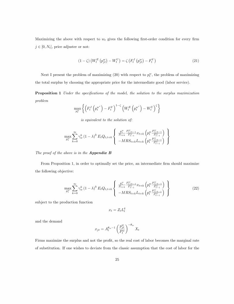
Next I present the problem of maximizing (20) with respect to pwt , the problem of maximizing

the total surplus by choosing the appropriate price for the intermediate good (labor service).

Proposition 1 Under the speci�cations of the model, the solution to the surplus maximization

problem

maxpwt

��F Jt

�pw

�

t

�� FVt

�1�� �WEt

�pw

�

t

��WU

t

���is equivalent to the solution of:

maxpwt

1Xk=0

kw (1� �)kEtQt;t+k

8><>:pwtPt+k

Pwt+k�1Pwt�1

xt+k

�pwt

Pwt+k�1Pwt�1

��MRSt+kLt+k

�pwt

Pwt+k�1Pwt�1

�9>=>;

The proof of the above is in the Appendix B

From Proposition 1, in order to optimally set the price, an intermediate �rm should maximize

the following objective:

maxpwt

1Xk=0

kw (1� �)kEtQt;t+k

8><>:pwtPt+k

Pwt+k�1Pwt�1

xt+k

�pwt

Pwt+k�1Pwt�1

��MRSt+kLt+k

�pwt

Pwt+k�1Pwt�1

�9>=>; (22)

subject to the production function

xt = ZtL�t

and the demand

xjt = A�w�1t

�pwjtPwt

���wXt

Firms maximize the surplus and not the pro�t, so the real cost of labor becomes the marginal rate

of substitution. If one wishes to deviate from the classic assumption that the cost of labor for the

25

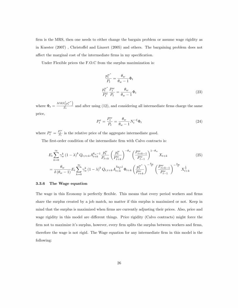
�rm is the MRS, then one needs to either change the bargain problem or assume wage rigidity as

in Kuester (2007) , Christo¤el and Linzert (2005) and others. The bargaining problem does not

a¤ect the marginal cost of the intermediate �rms in my speci�cation.

Under Flexible prices the F.O.C from the surplus maximization is:

pw�

t

Pt=

�w�w � 1

�t

pw�

t

Pwt

PwtPt

=�w

�w � 1�t (23)

where �t =MRS

�pw

�t

�Zt

and after using (12), and considering all intermediate �rms charge the same

price,

P xt =PwtPt

=�w

�w � 1N��t �t (24)

where P xt =Pwt

Ptis the relative price of the aggregate intermediate good.

The �rst-order condition of the intermediate �rm with Calvo contracts is:

Et

1Xk=0

kw (1� �)kQt;t+kA

�w�1t+k

pwtPt+k

�pwtPwt+k

���w �Pwt+k�1Pwt�1

�1��wXt+k (25)

=�w

� (�w � 1)Et

1Xk=0

kw (1� �)kQt;t+kA

�w�1�

t+k �t+k

�pw

�

t

Pwt+k

�� �w��Pwt+k�1Pwt�1

�� �w�

X1�

t+k

3.3.6 The Wage equation

The wage in this Economy is perfectly �exible. This means that every period workers and �rms

share the surplus created by a job match, no matter if this surplus is maximized or not. Keep in

mind that the surplus is maximized when �rms are currently adjusting their prices. Also, price and

wage rigidity in this model are di¤erent things. Price rigidity (Calvo contracts) might force the

�rm not to maximize it�s surplus, however, every �rm splits the surplus between workers and �rms,

therefore the wage is not rigid. The Wage equation for any intermediate �rm in this model is the

following:

26

wjtLjt = (1� �)�G (Ljt)

�t� Gu (lut )

�t+ bt

�+ �Kt#t + �

pwjtPtxjt (26)

The above expression is derived combining (21) along with (16), (17) and (18). The details are in

Appendix D.

The wage equation splits the surplus generated by the match. It includes terms that are match-

speci�c and others that depend on variables outside of the match, variables that re�ect the state of

the labor market. The �rst and last terms in the wage equation are the only ones that depend on the

match. The �rst match-speci�c term G(Ljt)�t

, is the disutility of labor in terms of the real good. More

hours of work implies more disutility from working therefore the worker needs to be compensated

more. This term is the wage that would prevail in the standard New Keynesian model without labor

market frictions. The last termpwjtPtxjt is the revenue of the �rm. Higher revenue creates higher

surplus from a match leading to higher wage. Those two terms are based on the characteristics

of the speci�c �rm and worker and they are match-speci�c. The remaining terms arise due to the

nature of the bargain. Workers theoretically have the option to break the negotiations with the

�rm and enter the unemployment pool if the wage bargain seems unfavorable. Hence, those terms

arise in the wage equation as outside opportunities that a¤ect the relative bargaining power of the

two sides. The less severe is the outside opportunity (unemployment value) the more bargaining

power is earned by the workers. The variable bt is the constant unemployment bene�t. Higher

unemployment bene�t makes the outside opportunity (value of unemployment to worker) higher,

which increases the bargaining power of the worker and entitles her to higher wage compensation.

As I already mentioned, #t =�tqt= Vt

1�Ntis the market tightness. The tightness #t, is high when

there are relatively more job openings than unemployed workers. In such case, for a worker to �nd

a job is more likely than a vacant job to �nd a match. High #t then, increases the bargain power

of workers again by improving outside opportunities (unemployment duration 1�tis low), earning a

higher wage, since workers are in relatively high demand. The extra termGu(lujt)�t

is the disutility of

search e¤ort in terms of the real good su¤ered by each unemployed worker in order to participate

in the job market. This term also captures the e¤ect of relevant others on the value of a worker�s

27

unemployment state, which is the psychological cost of being unemployed and searching. Again,

this term is associated with the outside opportunities of breaking the bargain.

Moreover, the appearance of marginal utility �t serves the same purpose as lut , since �t is also

a countercyclical variable. In an expansion, marginal utility is decreasing, implying that a utility

unit in a boom, corresponds to more units of the real good than one utility unit in a recession. If

the variety coe¢ cient was set to zero, �u = 0, every worker would put �xed e¤ort � every period.

A constant unit of e¤ort will require constant disutility Gu (�) per worker to participate in the

job market. However, this constant disutility, when transformed to units of the real good Gu(�)�t

becomes a procyclical variable that can, to some extend, counterbalance part of the change in

market tightness, enhancing the model�s ampli�cations.

The above wage expression is the wage equation for any �rm, price adjusting or not. Job creation

is a statement about the new �rms, therefore the wage relevant for vacancy posting is the wage of

a price adjusting �rm. However the wage response in the implied impulse responses is the average

wage of the whole economy. The aggregation of all possible wages in the economy is derived in

Appendix E.

3.4 Retail �rms

Retail �rms use the output of wholesale �rms to produce the �nal good. There is a continuum of

retail �rms with measure of one. Those �rms use as inputs the output of the wholesale �rms, and

produce according to the following production function

yit = ZrtXit

where Xit is the quantity of the composite intermediate good employed by the ith retail �rm. Each

of those retail �rms is producing a di¤erentiated product. Let chit be the demand for consumption

28

good i from the hth household. The aggregate consumption good for the hth household is:

Cht =

24 1Z0

ch��1�

it di

35�

��1

(27)

The underlying demand for consumption derived from the usual cost minimization problem is:

chit =

�pitPt

���Cht

The price of the composite good is the usual

Pt =

24 1Z0

p1��it di

351

1��

(28)

There�s nominal rigidity in the market for the �nal goods. A fraction of the �rms are allowed to

adjust their price each period. The ones that fail to adjust their price simply index their price to

the most recent in�ation rate.

A retail �rm currently adjusting it�s price is solving the usual Pro�t maximization problem:

maxpt

( 1Xk=0

kEtQt;t+k

�ptPt+k

Pt+k�1Pt�1

�1���MCt+k

�ptPt+k

Pt+k�1Pt�1

���!Yt+k

)

where MC is the retail �rm�s marginal cost, which is simply:

MCt =PwtPt

1

Zrt=P xtZrt

The marginal cost for the retail �rms is the price P xt the intermediate �rms charge for the aggregate

labor service Xt divided by the marginal product of labor9 . Under fully �exible prices, the above

necessary condition becomes:p�tPt=

�

� � 1MCt

9 In this case the marginal product is simply Zrt a common to all retail �rms productivity shock.

29

which means that the relative price each individual retail producer sets is a markup over marginal

cost.

From the aggregate price index (28) I get:

P 1��t = (1� ) p�1��

t + P 1��t�1

�Pt�1Pt�2

�1��(29)

3.5 Government and Monetary authority

The monetary authority conducts monetary policy following a Taylor rule. There in no government

spending in this model and the Government is following a Ricardian policy regime.

3.5.1 Government

The Government redistributes any amount raised from the issue of government bonds and revenue

from vacancy posting with the use of lump sum transfers and unemployment bene�ts. Every period

the government keeps a balanced budget. The government�s budget constraint is:

(1�Nt)Ptbt +Bt�1 (1 + it�1) = Bt +KtPtVt + Tt

Solving the government budget constraint for Tt and plugging it into the household�s budget con-

straint I get the aggregate resource constraint.

Ct = Yt

It is worth noting that the cost of vacancies KtVt appears in the household budget constraint but

not the resource constraint since the cost of vacancies in modeled as a tax cost.

3.5.2 Monetary authority

The monetary authority controls the nominal interest rate via a Taylor rule:

30

1 + it = (1 + it�1)�i

�PtPt�1

���(1��i)Y�y(1��i)t eut

The parameters �� and �y are the coe¢ cients determining the response of the Central Bank

to in�ation and output respectively. The coe¢ cient �i is measuring the degree of interest rate

smoothing, included in the Taylor rule following the empirical work of Clarida, Gali and Gertler

(2000). The variable ut is a monetary policy shock.

3.6 Equilibrium

Since all households are the same, in equilibrium I can ignore the index h. Also in equilibrium

Nwht = NF

ht = Nt, sht = 1 and I = 1.

The �rst-order conditions give the usual Euler equation

1

1 + it= �Et

�t+1�t

PtPt+1

(30)

where

�t = (Ct � �Ct�1)��

is the marginal utility. In equilibrium the household�s intermediate �rm ownership becomes the

usual law of motion for employment:

Nt+1 = (1� �)Nt +Ht (31)

where Ht is the matching function.

The resource constraint10 is:

Ct = Yt (32)

10Here we assume that the costs of vacancies is subsitized by the government, therefore those expenditure do notappear in the resource constraint. Trigari (2004), Walsh (2005) and Kuester (2007) make the exact same assumptionthat simpli�es the model especially the evaluation of its steady state.

31

From the �rst-order condition for vacancies arises the job creation condition

Kt

qt= (1� �)EtQt;t+1

Kt+1

qt+1+ EtQt;t+1�

wht+1

�pw

�

t

�(33)

The cost of posting a vacancy is Kt = kv

�VtVt�1

� . The reason of assuming adjustment costs

in vacancies is because the search and match framework does not explain the inertial response of

vacancies observed in the data. Vacancies and wages are jump variables in the standard MP setting.

Similar assumption for vacancy costs is made by Braun (2005).

Using the F.O.C of the intermediate �rm�s problem, equation (25) and the price of the aggregate

service (12) in log-linear form while �xing the elasticity of output to labor to � = 1 (my benchmark

calibration), I get an expression for intermediate good�s in�ation equation

�wt =1

1 + ��wt�1 +

�

1 + ��wt+1 + �

�mrst � P xt

�� �nnt +

�

1 + �nt�1 + �

�

1 + �nt+1 (34)

where � = 11+�

1� w(1��)1�� w(1��)

w(1��)1+`�w

, and �n =�

1+�1+� 2w(1��)

2

w(1��) ,

mrst = `Xt � �t + ` (�w � 1) At+k. All the steps for deriving the intermediate good Philips

curve are in Appendix B.

From the retail �rm�s �rst-order condition combined with (29), I get the usual Philips curve for

the evolution of �nal good in�ation:

�t =1

1 + ��t�1 +

�

1 + �Et�t+1 +

(1� ) (1� � ) (1 + �)

�P xt � zrt

�(35)

By de�nition the relative price of the intermediate good �rms is P xt =Pwt

Pt. Log-linearizing this, I

can express the price of the composite labor service, as a function of the intermediate and retail

good in�ation as follows

P xt = P xt�1 + �wt � �t�1

32

4 Calibration, estimation and results

I partition the parameters of the model into two sets. The �rst set of parameters is:

�1 = f�; �; �; �; �w; `; �; �; b; q; �; ; ��g

while the second set of parameters is:

�2 = f�; `u; �u; �; �; �; ; w; �i; �yg

I calibrate the �rst set of parameters �1 and I estimate the parameters in the second set �2 to match

the model implied impulse responses after a monetary shock, with the empirical responses obtained

from a structural VAR on U.S. data.

The �rst partition �1, contains parameters for which either microevidence exists, or those para-

meters are not too important for the models dynamics. The second partition �2, contains variables

that are either important for the model�s dynamics, or parameters for which microevidence is not

available.

4.1 Calibration

The performance criterion upon which I evaluate my model is whether it can match, up to an

acceptable extent, the impulse responses to a monetary shock, identi�ed in an SVAR on US data.

A summary of the calibrated parameters is presented in table 1. I calibrate the parameters of

the model to values from independent studies. I set the steady state probability a vacancy to be

matched, �q, to 0.7 like Cooley and Quadrini (1999) and den Haan, Ramey and Watson (2000).

I set the probability of a worker to �nd a job, ��, to 0.6, as Cole and Rogerson (1999) implying

an unemployment duration of 1.67 quarters. By picking those values for the two probabilities I

immediate pin down the value of the e¢ ciency of the match, h, to 0.6511 . I set the unemployment

11The variable h = ~h�� according to our de�nition of the matching function

33

bene�t b to zero12 , the lowest possible value, to make sure it is not driving my result13 .

The separation rate, �, to 0.035. This implies a 6% steady state unemployment level. Hall (1999)

estimates a value of 0.08 and usually values vary around 0.08-0.1. My choice of the separation rate

is not important in achieving my target. I use a discount rate, �, to 0.989, which implies a 1% real

interest rate per quarter. The elasticity of substitution for �nal goods, �, is set to 11, which entails

a markup of 1.1. The elasticity of substitution for the intermediate goods, �w, is set to 25. Boivin

and Giannoni (2005) propose a value of 11 and Altig, Christiano, Eichenbaum and Linde (2005) set

the own price elasticity of demand to 101. My value of �w = 25 lies in between the values proposed

in the literature. I set the risk aversion coe¢ cient, �, to 3. The inverse of labor supply elasticity, `,

is set to 10, which corresponds to a rather inelastic labor supply. It implies a labor supply elasticity

of 1` = 0:1. Trigari (2005) and Kuester (2005) use the same value. Card (1994) estimates that1` 2

(0; 0:5). My parameter value lies in the interval.

I set the value for the �nal good price rigidity, , to 0.5, along with evidence by Bils and Klenow

(2004) suggesting prices adjust on average every two quarters. I set the nominal rate response of

the central bank to in�ation, ��, to 1.1, as in Bernanke, Gertler and Gilchchrist (1999).

4.2 The estimation procedure

I use the techniques introduced by Rotemberg and Woodford (1999) to bring the model to the data.

I estimate a set of parameters in order to minimize the distance between model implied impulse

responses and the responses obtained from a structural VAR on US data. More weight is placed on

the most accurately estimated responses. The exact methodology is presented in detail below.

De�ne with �M () the vector valued function of the impulse responses from my model. It is a

function of the parameter vector . I denote with �V the vector of the impulse responses from the

12Setting b = 0:4 as in Shimer (2005) has a very small impact on the responses and estimated parameter and thisis one of my goals, to create a model that�s not too sensitive to unemployment bene�t changes.13A high value for the unemployment bene�t increases the steady state value of the wage while decreasing the

steady state of pro�ts. This decreases the deviation of wage from it�s steady state thus increasing vacancy volatility.This mechanism creates ampli�cation in Hagedorn and Manovskii (2007).

34

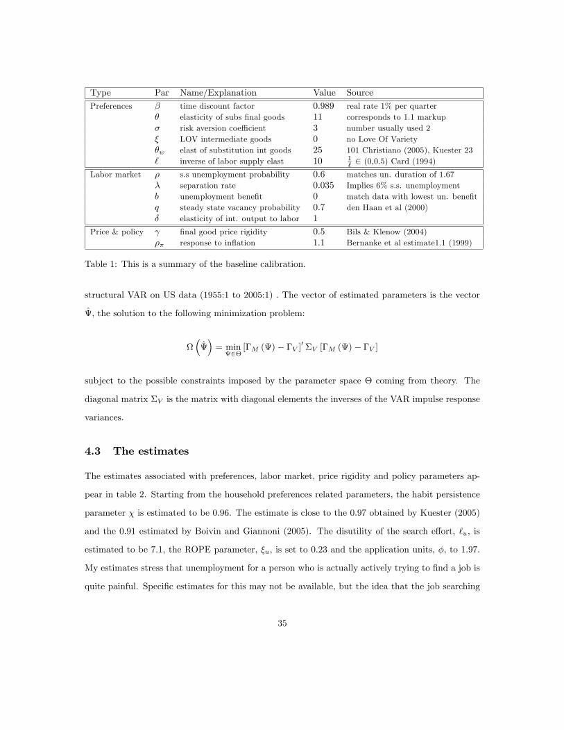
Type Par Name/Explanation Value Source

Preferences � time discount factor 0:989 real rate 1% per quarter� elasticity of subs �nal goods 11 corresponds to 1.1 markup� risk aversion coe¢ cient 3 number usually used 2� LOV intermediate goods 0 no Love Of Variety�w elast of substitution int goods 25 101 Christiano (2005), Kuester 23` inverse of labor supply elast 10 1

` 2 (0,0.5) Card (1994)Labor market � s.s unemployment probability 0:6 matches un. duration of 1.67

� separation rate 0:035 Implies 6% s.s. unemploymentb unemployment bene�t 0 match data with lowest un. bene�tq steady state vacancy probability 0:7 den Haan et al (2000)� elasticity of int. output to labor 1

Price & policy �nal good price rigidity 0:5 Bils & Klenow (2004)�� response to in�ation 1:1 Bernanke et al estimate1.1 (1999)

Table 1: This is a summary of the baseline calibration.

structural VAR on US data (1955:1 to 2005:1) . The vector of estimated parameters is the vector

, the solution to the following minimization problem:

��= min

2�[�M ()� �V ]0 �V [�M ()� �V ]

subject to the possible constraints imposed by the parameter space � coming from theory. The

diagonal matrix �V is the matrix with diagonal elements the inverses of the VAR impulse response

variances.

4.3 The estimates

The estimates associated with preferences, labor market, price rigidity and policy parameters ap-

pear in table 2. Starting from the household preferences related parameters, the habit persistence

parameter � is estimated to be 0.96. The estimate is close to the 0.97 obtained by Kuester (2005)

and the 0.91 estimated by Boivin and Giannoni (2005). The disutility of the search e¤ort, `u, is

estimated to be 7.1, the ROPE parameter, �u, is set to 0.23 and the application units, �, to 1.97.

My estimates stress that unemployment for a person who is actually actively trying to �nd a job is

quite painful. Speci�c estimates for this may not be available, but the idea that the job searching

35

Type Par Name/explanation Value st.dev.

Preferences � habit persistence 0:96 (0:002)`u disutility of search e¤ort param. 7:1 (0:073)�u ROPE coe¢ cient 0:23 (0:003)� application units per person 1:97 (0:026)

Labor Market � elast. matching function 0:46 (0:019)� workers bargaining power 0:81 (0:009) vac adjustment cost parameter 4:1 (0:413)

Price & policy w intermediate good price rigidity 0:55 (0:031)�i policy inertia 0:83 (0:005)�y policy response to output 0:2 (0:064)

Table 2: The table presents the estimated parameters from the minimum distance procedure tomatch the model implied impulse responses with the empirical. The numbers in parenthesis arestandard deviations.

experience to involve frustration, stress and inevitably high disutility seems reasonable.

For the labor market parameters, the elasticity of the matching function, �, is set to 0.45, close

to the value of 0.4 estimated by Blanchard and Diamond (1989). Petrongolo and Pissarides (2001)

estimate the elasticity of the matching function with respect to unemployment to be between 0.5-

0.7. My estimate lies a little lower than their bound. The share of the surplus that goes to workers,

�, is estimated in my model to 0.8. Although there are no microevidence for this parameter it is

close to 0.77 obtained by Braun (2005). Trigari (2004) estimates � = 0:81, while Kuester (2005)

�nds � = 0:21 and Shimer (2005a) calibrates it to 0.7. The vacancy adjustment cost, , is estimated

to be 4.1 and Braun estimates it to be around 2.

My estimate of price rigidity, w, is 0.55 close to 0.5 suggested by Bils & Klenow (2004). For

the intermediate goods Christiano et al. (2005) �nd an estimate for w = 0:64. For the policy

parameters, I �nd the policy inertia parameter, �i, to be 0.83 as in Kuester (2005) and close

to Trigari�s (2004) estimate of 0.85. The policy inertia parameter is important for the size and

persistence of the responses. An extended discussion about this fact can be found in Walsh (2005).

The monetary authority�s policy response to output �y is estimated to be 0.2. Both policy values

are mostly in line with the �ndings of Clarida, Gali and Gertler (2000).

36

4.4 The model�s ability to match the data

I present the model implied along with the empirical impulse responses of the variables of interest

after a unit monetary shock in �gure 4. The solid lines represent the responses obtained from

running a VAR on quarterly US data from 1955:1 to 2005:1, which are the same as the ones in

�gure 1. The solid lines with bullet marks represent the model implied responses, and the gray

areas are 90% con�dence intervals. The model�s responses are consistent with the persistence and

cyclicality of various key macroeconomic variables in the data.

The model-predicted response of in�ation is as low and inertial as it�s empirical counterpart.

The model implied responses of vacancies, unemployment and job creation can match the level of

magnitude, as well as the persistence of the responses observed in the data.

The low and inertial response of the real wage is matched fairly well, despite the tendency of

search and matching models augmented with monetary shocks to overshoot the responses of the

real wage. Below I provide details as to how my di¤erent assumptions contribute to the picture in

�gure 4.

4.5 The main ingredients

I refer to as main ingredients, the two key departures from the literature that I�ve already stated

in the introduction, which are the introduction of unemployment as a social norm and nominal

rigidities in the intermediate sector. The e¤ect of each of my key assumptions on the �t of the model

in �gure 4 is discussed below, as well as the performance of the model when those mechanisms are

excluded.

4.5.1 The introduction of unemployment as a social norm

Figure 4 shows that the model can create enough ampli�cation for vacancies, unemployment and

job creation. The volatilities of those variables are ampli�ed by the introduction of unemployment

as a social norm. As I�ve already covered, after an expansionary monetary shock, the unemployment

of relevant others is declining, while marginal utility is decreasing. According to the norm, and the

37

decreasing marginal utility, the searching experience by each individual job seeker becomes more

unpleasant, which lowers the value of unemployment for a worker who eventually looses bargaining

power. The loss of bargaining power, hinders the wage from responding too much to the increased

likelihood of �nding a job elsewhere, boosting this way vacancy creation.

Figure 5 shows the optimal �t14 of the model without the social norm assumption (� = 0). I

do not present responses other than vacancies, unemployment and job creation because the model

performs fairly well in explaining those15 . Clearly the model cannot create the ampli�cation needed

without the social norm speci�cation which means that a non-zero � and the ROPE parameter �u

play an important role in the labor market variables�volatilities. However, some ampli�cation is

present in the model without the social norm, since the addition of a monetary side can supply the

model with some extra volatility for vacancies and unemployment as also stressed by Barnichon

(2007). The addition of a monetary side can boost the present value of �rm pro�ts via interest

rate changes that directly a¤ect the stochastic discount factor. In other words, in an expansion the

interest rate drops and the stochastic discount factor increases, inducing vacancy creation through

higher present value of future cash �ows.

To further motivate the importance of my model�s job market framework, I present some re-

sponses to a unit monetary shock for di¤erent degrees of ROPE, �u, that governs the importance of

the measure of the supporters of the norm to the disutility of the code breakers. Figure 6 examines

the e¤ect on the model implied responses using my benchmark calibration for di¤erent values of

ROPE. It is distinct that higher degrees of the ROPE parameter �u, can amplify the responses of

vacancies, unemployment and job creation in the model.

I proceed by setting �u = 0 and simply vary the value of application units per person �, to

observe how the countercyclicality of marginal utility can also create a procyclical response for the

perceived search e¤ort and therefore enhance the ampli�cation of the shocks in my model. Figure

7 shows the response of vacancies, unemployment and job creation after a unit monetary shock, by

varying the application units �, while keeping ROPE equal to zero. It is evident that by simply

14By optimal �t I mean running the algorithm in order to match the empirical responses subject to parameterconstraints coming from micro evidence. The �t of the model compare to the empirical responses is my measure ofsuccess.15This is expected since the ampli�cation puzzle a¤ects primarily those three variables in this model.

38

assuming the search cost is denominated in e¤ort units instead of units of the �nal good (as usually

assumed in the literature), ampli�cation can be improved in the model.

Despite the fact that the countercyclicality of both the psychological cost of unemployment and

the marginal utility contribute in ampli�cation of the shocks in my model, the cyclicality of the

marginal utility alone cannot create the ampli�cation needed in the data. This can be motivated

by looking at �gure 8 which shows the optimal �t of the model by keeping �u = 0 and letting the

cyclicality of the marginal utility alone to provide ampli�cation. I only present the labor market

variables since the remaining responses can match the empirical ones fairly well. The marginal

utility alone cannot provide enough ampli�cation especially for vacancies and job creation. Also

a large number is needed for the vacancy adjustment cost parameter. This result speci�es that

both e¤ects are important, even though the social norm assumption is more vital in boosting

ampli�cation.

4.5.2 The introduction of price stickiness in the intermediate sector

The assumption of price stickiness of the form of Calvo contracts is very important in this model.

The purpose of this assumption is twofold. On the �rst hand it aims in enhancing the model�s

persistence and on the other hand to lower the volatility of the wage response after a monetary

shock.

Many authors like Gertler and Trigari (2006), Shimer (2005b) and others have used wage rigidity

for new �rms, to obtain ampli�cation, an assumption that is rejected for it�s empirical validity by

Pissarides (2007) and Haefke, Sonntag and van Rens (2008). Wage rigidity for new matches might

be rejected by the evidence, but what about wage rigidity for continuing �rms? Wage rigidity, at

least for continuing �rms, seems to be essential to guarantee the low and inertial response of the real

wage observed in the data. The only problem is that, according to Krause and Lubik (2005), the

wage rigidity assumption could aid me in matching the wage response, but the assumption will not

contribute at all in obtaining in�ation inertia. As the authors report, this is because the partition

of the production activity in two sectors, makes the retail �rm�s marginal cost una¤ected by wage

rigidity in intermediate sector, leaving the in�ation response barely a¤ected.

39

Instead, the assumption of price rigidity for intermediate �rms, not only enables the model

to match the real wage response, but also creates additional in�ation inertia. Calvo pricing in

the intermediate sector, enables me to take advantage of the assumption that every worker is an

intermediate �rm, to boost the in�ation inertia and persistence implied by the model. Since an

intermediate �rm currently adjusting it�s price uses a single worker�s labor hours in production,

the �rm takes into consideration how the price of labor is directly a¤ected by the �rm�s pricing

decision. In an expansion, when a price adjusting �rm considers increasing it�s price, the demand

for it�s product must fall. The fall in demand induces a fall in demand for labor hours, which implies

a lower disutility of labor for the worker and therefore a lower marginal cost for the �rm, which

applies pressure on the price initially set by the �rm to decrease. Stated otherwise, an attempt of

an intermediate �rm to increase it�s price, triggers a mechanism that tends to decrease the initial

price change. Thus, the changes in prices are achieved in smaller increments, increasing the degree

of strategic complementarity between intermediate �rms and eventually induce smaller adjustments

in marginal costs faced by retail �rms. This is an e¤ective way of increasing in�ation inertia in

the model. Treating each worker as a single �rm will add the term 1 + `�w in the denominator of

the parameter � in the Philips curve for the intermediate goods (34), that tends to decrease the

volatility of intermediate good in�ation and justi�es my choice of a fairly inelastic labor supply

(inverse of labor supply elasticity ` calibrated to 10). A discussion about the di¤erence between

�rms employing a single worker against employing partly all workers in the economy can be found

in chapter 3 of Woodford (2003).

Therefore, price rigidity in intermediate �rms allows me to increase the real rigidity in the model.

The important question now is: can the model match the data by simply assuming price rigidity

only in the retail sector? To answer this question, I set the parameter governing the degree of price

stickiness in the intermediate sector, w, to zero, while letting the degree of price rigidity for retail

�rms, , to vary. In addition, I remove the social norm assumption temporarily for this speci�cation.

In other words, in this exercise, there�s only rigidity in the retail sector, while intermediate �rms

have �exible prices. Figure 9 shows the optimal �t of that model for three di¤erent speci�cations.

The lines with dot marks correspond to the optimal �t when is estimated with no restriction

40

imposed on the parameter. The lines with circle marks and star marks, correspond to the same

exercise with calibrated to 0.85 and 0.55 respectively. The estimated degree of price rigidity for

the �rst speci�cation is: = 0:97, an implausible value according to evidence by Bils and Klenow

(2004).

What might strike you as unusual is that the responses with the dot mark can actually cre-

ate enough ampli�cation without the need of the social norm assumption. According to Andres,

Domenech, and Ferri (2006), in a model with two sectors, increases in the degree of price rigidity

can create ampli�cation. This is due to the fact that the intermediate �rm�s revenue depends on the

relative price pwt

Pt, where pwt is the price of the intermediate �rm and Pt the price of the consumption

good. In an expansion, additional rigidity in intermediate �rms, lowers the volatility of the price of

the consumption good Pt, therefore, the relative price of intermediate �rms�signi�cantly increases,

boosting �rm pro�ts and vacancy creation16 . However, when the degree of price rigidity assumed

for retail �rms is reduced to more acceptable values, the lines with the circle and star marks in

�gure 9 show that not only the persistence in the model disappears, but also the ampli�cation,

which can be only sustained by values of greater than 0.9.

In addition, �gure 9 shows that whichever value for is used, the model with �exible interme-

diate �rms overshoots the wage responses, an observation also shown in Christiano, Trabandt and

Walentin (2009). Thus, it is evident from the above exercise that the assumption of price rigidity

in the intermediate sector is vital for preventing the wage from being too volatile after a monetary

shock.

Other than the wage, the remaining responses with star and circle marks, can match nearly none

of the empirical responses. This means that when more reasonable values for retail price rigidity

are assumed, the model�s performance is not even close to satisfactory. A model with �exible

intermediate �rms and no social norm framework cannot account for the empirical responses. The

question now is: can a model with �exible intermediate �rms augmented with the social norm

assumption, account for the data without the assumption of price rigidity in intermediate �rms?

The answer to this question is provided in �gure 10. Clearly the model cannot match the responses,16 In my model this e¤ect doesn�t exist since the rigidity is in both sectors, therefore there is no signi�cant change

in relative price.

41

even though the social norm assumption seems to create at least the appropriate ampli�cation for

vacancies, unemployment and job creation. The response of in�ation is not persistent enough,

stressing the necessity of price rigidity in the intermediate sector that can induce greater in�ation

inertia and persistence in the model.

Therefore, both the assumptions of price rigidity in intermediate �rms and unemployment as a

social norm are indispensable ingredients for my model�s performance.

4.5.3 Other ingredients

The output response in �gure 4 is inertial and persistent. This is achieved through the employment

of habit persistence in preferences. The real hourly wage is also in-line with the data. The response

of the real wage is about half the response of output, along with the estimates of Giannoni and

Woodford (2005). The small and inertial response of the real wage comes from the nominal rigidities

in the intermediate sector. First of all, because the new �rms are price adjusters in the �rst period,

they face a decline in demand when increasing their price and employ less labor hours in production.

Thus, in the wage equation, the revenue of the new �rm, which is a part of the wage (last term in

(26)), is negative during an expansion. The disutility of labor (�rst term in (26)) is also negative

due to the declining demand the price adjusting �rm is facing. On aggregate, this lowers the average

wage in the economy. In the standard MP model with monetary shocks, the wage tends to be way

too volatile. Similar discussion as to how to lower the wage implied by a search and matching

framework with market power, can be found in Rotemberg (2006).

An important role towards my goal is the assumption of adjustment costs in vacancies, Kt =

kv

�VtVt�1

� . The necessity of this assumption stems from the forward looking nature of the job

creation condition, equation (19). Since �rm exit in the model is quite low (as it should be according

to evidence), there is no restriction in the model as to when the intermediate �rms should be created.

There is a tendency for the vacancies to be posted all at once and employment to reach it�s peak

fairly early. However, the adjustment costs account for the inertial response of vacancies observed in

the data. This kind of vacancy cost can be obtained by assuming time to build in vacancy creation

as assumed for jobs in this model. Lucca (2005) creates a framework where a vacancy cost of the

42

type I already assumed rises. In �gure 11, I examine the �t of the model by assuming no vacancy

adjustment costs. It is apparent that vacancies respond immediately and unemployment reaches

it�s pick fast. Thus, the assumption of vacancy adjustment costs is crucial for vacancy inertia and

persistence. However, assuming vacancy adjustment costs, sacri�ces ampli�cation for persistence

in the model, which implies that the virtues of the vacancy adjustment cost assumption can only

be prominent in a model employed with a good ampli�cation mechanism.

5 Conclusion

I have presented a fairly simple new Keynesian model with search unemployment to explain the

joint response of key macroeconomic variables after a monetary shock. My main departure is the

introduction of unemployment as a social norm that incorporates the belief that the unemployed

are a burden to society, resulting in additional pressure from households upon the unemployed to

�nd a job. The lower the unemployment within the household raises the support of the norm and

the greater the pressure is upon the individual unemployed. This extra psychological cost imposed

by the norm counterbalances the bargaining power gained by decreasing unemployment duration

during an expansion, preventing the wage from crowding out vacancy creation, boosting the model�s

ampli�cation mechanism.

I also assume nominal rigidities (Calvo contracts) in the intermediate good sector (labor market)

in order to create enough persistence in the model. Price rigidity in the intermediate sector not

only contributes in creating in�ation inertia but also aids me in keeping the wage response low and

smooth. In a monetary model with no nominal rigidities in the labor market, the wage implied is

too volatile.

The model can match the impulse responses implied by a structural VAR on quarterly US data

from 1955:1 to 2005:1 and can be used for optimal monetary policy analysis. My goal was to match

the data by assuming moderate degrees of price rigidity and without the aid of wage rigidity or

unreasonable calibration, mechanisms that have been heavily criticized recently. In other words, I

tried to address the Shimer puzzle by employing monetary shocks and at the same time avoiding

43

stickiness in wages and high unemployment bene�ts.

In addition, there is an interesting interaction between the in�ation process and the search and

match framework created by the appearance of the extensive margin in the labor market, which

can be important for policy analysis. As a matter of fact, the ultimate goal of my paper is to show

that the model can perform well according to the facts, in order to apply the model for optimal

monetary policy design and welfare analysis. I intend to consider those extensions in the future.

Moreover, there is an interaction between the model�s dynamics and the degree of Love Of

Variety (LOV), �, that I wish to further investigate, as the degree of in�ation inertia can be linked

to this parameter and also the evolution of intermediate �rms.

At last, I�m interested in investigating the case where the number of application units per period

� is variable and constitutes a choice variable for the household, in an attempt to address puzzles

associated with search intensity.

References

[1] Akerlof, G., (1980). "A theory of Social Custom, of which Unemployment may be one Custom",

Quarterly Journal of Economics 94(4), 749-775.

[2] Akerlof, G., (2006). "The Missing Motivation in Macroeconomics", American Economic Review

97, 5-36.

[3] Altig D. Christiano L., Eichenbaum M. and Linde J. (2011). "Firm-Speci�c Capital, Nominal

Rigidities and the Business Cycle," Review of Economic Dynamics, Elsevier for the Society for

Economic Dynamics, vol. 14(2), pages 225-247, April.

[4] Andolfatto, D., (1996). "Business Cycles and Labor Market Search", American Economic

Review 861, 112-132.

[5] Andres, J., R. Domenech, and J. Ferri (2006). "Price Rigidity and the Volatility of Vacancies

and Unemployment", mimeo, Universidad de Valencia, March.

44

[6] Barnichon, R., (2007). "The Smimer Puzzle and the Correct Identi�cation of Productivity

Shocks", mimeo, LSE, August.

[7] Benassy, J-P., (1996). "Taste for Variety and Optimum Production Patterns in Monopolistic

Competition", Economic Letters 52, 41-47.

[8] Bernanke, B., M. Gertler, and S. Gilchrist (1999). "The Financial Accelerator in a Business

Cycle Framework", Handbook of Macroeconomics, J. Taylor and M. Woodford, editors.

[9] Bils, M., and P. Klenow (2004). "Some Evidence in the Importance of Sticky Prices," Journal

of Political Economy , 112(5), 947-985.

[10] Boivin, J., and M. P. Giannoni (2005). "Has Monetary Policy Become More E¤ective?", NBER

Working Paper No. 9459

[11] Braun, H. (2005). "(Un)employment Dynamics: The Case of Monetary Policy Shocks", mimeo;

Northwestern University.

[12] Calvo, Guillermo (1983). "Staggered Prices in a Utility Maximizing Framework", Journal of

Monetary Economics 12, 383-398.

[13] Cardullo, G., (2008). "Matching Models Under Scrutiny: Understanding the Shimer Puzzle",

Discussion Papers, Department des Sciences Economiques 2008009.

[14] Christiano, L. J., M. Eichenbaum, and Evans (2005). "Nominal Rigidities and the Dynamic

E¤ects of a Shock to Monetary Policy", Journal of Political Economy, 113(1), 1-45.

[15] Christiano L. J., M. Trabandt, and K. Walentin (2009). "DSGE Models for Monetary Policy",

Handbook on Monetary Economics, edited by Friedman and Woodford, forthcoming.

[16] Christo¤el, K., and T. Linzert (2005). "The Role of Real Wage Rigidity and Labor Market

Frictions for In�ation and Unemployment Dynamics", European Central Bank Working Paper

No. 556.

45

[17] Clarida, R., J. Gali, and M. Gertler (2000). "Monetary Policy Rules and Macroeconomic

Stability: Evidence and Some Theory", Quarterly Journal of Economics, 115,147-180.

[18] Clark, A.E., (2003). "Unemployment as a Social Norm: Psychological Evidence from Panel

Data", Journal of Labor Economics 21, 323-351.

[19] Clark, A.E., (2009). "Works, Jobs and Well-Being Across the Millennium", OECD Social,

Employment and Migration Working Papers 83.

[20] Clark, A.E., and A. J. Oswald (1994). "Unhappiness and Unemployment", Economic Journal

104, 648-659.

[21] Clark, A., A. Knabe and S. Ratzel (2009). �Unemployment as a social norm in Germany�,

Schmollers Jahrbuch (forthcoming)

[22] Cole, H., and R. Rogerson (1999). "Can the Mortenses-Pissarides matching model match the

business cycle facts?", International Economic Review 40(4), 933-959.

[23] Cooley, T.F., and V. Quadrini (1999). "A Neoclassical Model of the Philips Curve Relation",

Journal of Monetary Economics 44(2), 165-193.

[24] Costain, J., and M. Reiter (2007): �Business Cycles, Unemployment Insurance, and the Cali-

bration of Matching Models�, Journal of Economic Dynamics and Control, forthcoming.

[25] Davis S., J. Haltiwanger, and S. Schuh (1996). Job Creation and Destruction, The MIT Press.

[26] Den Haan, W., G. Ramey, and J. Watson (2000). "Job destruction and Propagation of Shocks",

American Economic Review, 90(3), 482-498.

[27] Dixit, A. K., and J. E. Stiglitz, (1977) "Monopolistic Competition and Optimum Product

Diversity", American Economic Review 6(3), 297-308.

[28] Gertler, M., and A. Trigari (2006). "Unemployment Fluctuations with Staggered Nash Bar-

gaining", New York University, April, mimeo.

46

[29] Fujita, S., (2003). "The Beveridge Curve, Job Creation and the Propagation of Shocks", mimeo,

University of California San Diego.

[30] R. E. Hall, (1999). "Labor-Market Frictions and Employment Fluctuations", NBER Working

Papers 6501, National Bureau of Economic Research, Inc.

[31] Haefke, C., M. Sonntag, and T. Van Rens (2007). "Wage Rigidity and Job Creation", mimeo,

July.

[32] Hagedorn, M., and I. Manovskii (2005). "The Cyclical Behavior of Equilibrium Unemployment

and Vacancies Revisited", American Economic Review, forthcoming.

[33] Jackson, P., and P. Warr (1987). "Mental Health of Unemployed Men inDi¤erent Parts of

England and Wales", British Medical Journal 295, 525.

[34] Krause, M., and Lubik (2005). "The (Ir)relevance of Real Wage Rigidity in the New Keynesian

Model with Search Frictions", Journal of Monetary Economics, forthcoming.

[35] Kuester, K., (2007). "Real Price and Wage Rigidities in a Model with Matching Frictions",

European Central Bank, working paper 720.

[36] Lucca, D., (2005). "Resusciating Time-To-Build", mimeo, Northwestern University.

[37] Mertz, M., (1995). "Search in the Labor Market and the Real Business Cycle", Journal of

Monetary Economics 36, 269-300.

[38] Mortensen, D., and C. Pissarides (1994). "Job Creation and Job Destruction in the Theory of

Unemployment", Review of Economic Studies 61, 397-415

[39] Neeleman, J., (1998). The Social and Epidemiological Context of Suicidal Behaviour, Gronin-

gen: University of Groningen Press.

[40] Pissarides, C., (2000). Equilibrium Unemployment Theory, The MIT Press.

[41] Pissarides, C., (2007). "The Unemployment Volatility Puzzle: Is Wage Stickiness the Answer?",

mimeo, London School of Economics, November.

47

[42] Platt, S., and N. Kreitman (1990). "Long Term Trends in Parasuicide and Unemployment in

Edinburgh, 1968-87", Social Psychiatry and Psychiatric Epidemiology 25, 56-61.

[43] Platt, S., R. Micciolo and M. Tansella (1992). "Suicide and Unemployment in Italy: Descrip-

tion, Analysis and Interpretation of Recent Trends", Social Science Medicine 34, 1191-1201.

[44] Powdthavee, N., (2007). "Are There Geographical Variations in the Psychological Cost of

Unemployment in South Africa?", Social Indicators Research 80, 629-652.

[45] Rotemberg, J., (2006). "Cyclical Wages in a Search-and-Bargaining Model with Large Firms",

CEPR, Discussion paper 5791.

[46] Rotemberg, J., and M. Woodford (1997). "An Optimization-Based Econometric Framework

for the Evaluation of Monetary Policy", NBER Macroeconomics Annual, 345-370.

[47] Shields, M., W. S. Price (2005). "Exploring the Economic and Social Determinants of Psycho-

logical and Psychosocial Health", Journal of the Royal Statistical Society 168, 513-538.

[48] Shields, M., W. S. Price and M. Wooden (2005). "Life Satisfaction and the Economic and

Social Characteristics of Neighbourhoods", Journal of Population Economics, (forthcoming).

[49] Shimer, R., (2005a). "The Cyclical Behavior of Equilibrium Unemployment, Vacancies, and

Wages: Evidence and Theory", American Economic Review 95(1), 25-49.

[50] Shimer, R., (2005b). "The Concequences of Rigid Wages in Search Models", Journal of Euro-

pean Association (Papers and Proceedings), 2, 469-479.

[51] Smets , F., and R. Wouters (2003). "An Estimated Stochastic Dynamic General Equilibrium

Model of the Euro Area", Journal of the European Economic Association 1(5), 1123-75.

[52] Stutzer, A., and R. Lalive (2004). "The Role of Social Norms in Job Searching and Subjective

Well-Being", Journal of the European Economic Association 2, 696-719.

[53] Trigari, A., (2004). "Equilibrium Unemployment, Job Flows and In�ation Dynamics", Journal

of Money, Credit and Banking 41(1), 1-33.

48

[54] Trigari, A., (2006). "The Role of Search Frictions and Bargaining for In�ation Dynamics",

IGIER Working Paper No. 304.

[55] Walsh, C., (2005). "Labor Market Search, Sticky Prices, and Interest Rate Policies", Review

of Economic Dynamics 8, 829-849.

[56] Woodford, M,. (2003): Interest and Prices, Princeton University Press, Princeton.

A Appendix

This part derives more formally my labor market speci�cation by de�ning the �rm that aggregates

the individual search e¤orts more properly. There is a �rm that combines household�s unemployed

workers� individual e¤ort and sells it to households. The household uses this aggregate e¤ort to

provide the needed application units to send it�s unemployed workers to the job market.

I assumed that each household demands FhD

t = �Uwht application units in order to have their

unemployed workers participate in the job market, where Uwht = I�Nwht is the number of unemployed

workers in the household. The household needs Luht aggregate e¤ort units to produce the aggregate

application units using the following production function FhS

t = Luht. There is a �rm that takes

unemployed workers�individual e¤ort and transforms it to aggregate e¤ort units according to the

following production function:

Luht = Aut

24ZUt

lu �u�1�u

hjt dj

35�u

�u�1

where

Aut � U�u� 1

�u�1t

The pro�t maximization problem of the �rm is:

maxluhjt

P lhtLuht �

ZUt

plhjtluhjtdj

49

s:t: Luht = Aut

24ZUt

lu�u�1�u

hjt dj

35�u

�u�1

The pro�t maximization problem derives the demand for individual e¤ort units:

luhjt = Au�u�1

t

plhjtP lt

!��uLuht

and

P lht =1

Aut

24ZUt

pl1��uhjt dj

35 11��u

Since all �rms are the same the above conditions become:

plhjt = U�ut P lt (36)

and

luhjt = U�(1+�u)t Luht (37)

I return to the household problem to de�ne our job market framework more formally. The

utility function of the household is the following:

WH (t) = maxfCht;Bht;Vhtg

8>><>>:U (Cht � �Ct�1)�

RNwht

G (Lhjt) dj �R

I�Nwht

Gu (luhkt) dk

+�EtWH (t+1)

9>>=>>;

50

The budget constraint is:

PtCht +Bht +KtPtVht + PltF

ht =Z

Nwht

WhjtLhjtdj +

ZI�Nw

ht

plhktLuhktdk

+ (I �Nwht)Ptb+ Tht + Ptsht

1Z0

�itdi

+ Pt

ZNFht

�whstds+ (1 + it�1)Bht�1

where Fht = �Uht = � (I �Nwht)

and

Nwht+1 = (1� �)Nw

ht + �t (I �Nwht)

The envelope condition with respect to Nwht determines the value of the job to the household,

important ingredient for the wage equation.

WHNwht(t) = �G (Lhjt) +Gu

�luhjt�+ �t�P

lt � �tplhktLuhjt + �t (WhjtLhjt � Ptb)

+ (1� �� �t)�EtWHNwht+1

(t+1)

Let�s simply focus on what is new in the above expression and keep in mind than in equilibrium

household speci�c variables are equal to the economy wide variables. What�s new in the above

equation is the following sum (after dividing everything by marginal utility):

NT =1

�t

�Gu (lut ) + �t�P

lt � �tpltlut

�=

1

1 + `u

lu1+`u

t

�t+ �

P ltPt� pltPtlut (38)

where �t = �tPt

51

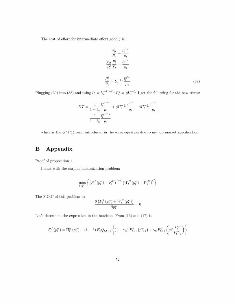
The cost of e¤ort for intermediate e¤ort good j is:

pljtPt

=lu

`u

t

�t

pljtP lt

P ltPt=lu

`u

t

�t

P ltPt= U��ut

lu`u

t

�t(39)

Plugging (39) into (38) and using lut = U�(1+�u)t Lut = �U��ut I get the following for the new terms:

NT =1

1 + `u

lu1+`u

t

�t+ �U��ut

lu`u

t

�t� �U��ut

lu`u

t

�t

=1

1 + `u

lu1+`u

t

�t

which is the Gu (lut ) term introduced in the wage equation due to my job market speci�cation.

B Appendix

Proof of proposition 1

I start with the surplus maximization problem:

maxfpwt g

n�F Jt (p

wt )� FVt

�1�� �WEt (p

wt )�WU

t

��o

The F.O.C of this problem is:@�F Jt (p

wt ) +W

Et (p

wt )�

@pwt= 0

Let�s determine the expression in the brackets. From (16) and (17) is:

F Jt (pwt ) = �

wt (p

wt ) + (1� �)EtQt;t+1

�(1� w)F Jt+1

�pwt+1

�+ wF

Jt+1

�pwt

PwtPwt�1

��

52

WEt (p

wt ) = wtLt �

$G (Lt)

�t+ EtQt;t+1

8><>: (1� �) (1� w)WEt+1

�pwt+1

�+ w (1� �)WE

t+1

�pwt

Pwt

Pwt�1

�+ �WU

t+1

9>=>;adding the two together and plugging in the equation for Pro�ts of the intermediate �rms�wt

�pw

�

t

�=

pw�

t

Ptxt � wtLt, the above becomes

F Jt (pwt ) +W

Et

�pw

�

t

�=pwtPtxt �

$G (Lt)

�t+ �EtQt;t+1W

Ut+1

+ (1� �)EtQt;t+1

8><>: (1� w)�F Jt+1

�pwt+1

�+WE

t+1

�pwt+1

��+ w

�F Jt+1

�pwt

Pwt

Pwt�1

�+WE

t+1

�pwt

Pwt

Pwt�1

��9>=>;

If I solve the equation forward, eliminating the terms F Jt+k (pwt ) +W

Et+k (p

wt ) for k = 1; :::;1 I get

F Jt (pwt ) +W

Et (p

wt ) = (40)

1Xk=0

kw (1� �)kEtQt;t+k

8><>:pwtPt+k

Pwt+k�1Pwt�1

xt+k

�pwt

Pwt+k�1Pwt�1

��$G

�Lt+k

�pwt

Pwt+k�1Pwt�1

���t+k

9>=>;+ (1� �) (1� w)

1Xk=0

kw (1� �)kEtQt;t+k+1

8><>: F Jt+k+1�pwt+k+1

�+WE

t+1

�pwt+k+1

�9>=>;

+ �

1Xk=0

kw (1� �)kEtQt;t+k+1W

Ut+k+1

The above expression is the expression in the brackets of the F.O.C I found before

@�F Jt (p

wt ) +W

Et (p

wt )�

@pwt= 0 (41)

Since the last two summations in (40) are independent of pwt , implying that after plugging (40) in

(41) I get:

@

0@ 1Pk=0

kw (1� �)kEtQt;t+k

8<: pwtPt+k

Pwt+k�1Pwt�1

xt+k

�pwt

Pwt+k�1Pwt�1

��

$G

�Lt+k

�pwt

Pwt+k�1Pwt�1

���t+k

9=;1A

@pwt= 0

53

which is equivalent to:

@

� 1Pk=0

kw (1� �)kEtQt;t+k

npwtPt+k

Pwt+k�1Pwt�1

xt+k

�pwt

Pwt+k�1Pwt�1

�o� $GL(Lt+k)

�tLt+k

�pwt

Pwt+k�1Pwt�1

��@pwt

= 0

and by de�ning MRSt =$GL(Lt+k)

�t+k, the above is the solution to a maximization problem like the

following:

maxpwt

1Xk=0

kw (1� �)kEtQt;t+k

�pwtPt+k

Pwt+k�1Pwt�1

xt+k

�pwtPwt+k�1Pwt�1

��MRSt+kLt+k

�pwtPwt+k�1Pwt�1

��

C Appendix

I�ll derive the Philips curve for the intermediate �rm�s in�ation. The FOC of the intermediate �rm�s

problem is:

Et

1Xk=0

kw (1� �)kQt;t+kA

�w�1t+k

pwtPt+k

�pwtPwt+k

���w �Pwt+k�1Pwt�1

�1��wXt+k

=�w

� (�w � 1)Et

1Xk=0

kw (1� �)kQt;t+kA

�w�1�

t+k �t+k

�pw

�

t

Pwt+k

�� �w��Pwt+k�1Pwt�1

�� �w�

X1�

t+k

The �rst-order condition can be rewritten as:

(�w � 1)Et1Xk=0

kw (1� �)kQt;t+kA

�w�1t+k P xt+k

�pw

�

t

Pwt

PwtPwt+k

�1��w �Pwt+k�1Pwt�1

�1��wXt+k

=�w�Et

1Xk=0

kw (1� �)kQt;t+kA

�w�1�

t+k X1�

t+k�t+k

�pw

�

t

Pwt

PwtPwt+k

�� �w��Pwt+k�1Pwt�1

�� �w�

where P xt =Pwt

Pt

De�ne Gwt =pw

�t

Pwt. Log-linearizing the above and using (23) at the steady state:

(�w � 1) �P x �A(�w�1)��1�

��Gw�1+�w 1��

� �X��1� =

�w��� (42)

54

I get

Et

1Xk=0

�k kw (1� �)k

0BBBB@(�w � 1) At+k + P xt+k + (1� �w) gwt+�1� �w + �w

�

� �Pwt � Pwt�1

�+(1� �w)

�Pwt+k�1 � Pt+k

�+�1� 1

�

�Xt+k

1CCCCA (43)

= Et

1Xk=0

�k kw (1� �)k

�'t+k +

�w � 1�

At+k ��w�gwt �

�w�

�Pwt+k�1 � Pt+k

��

Hat variables are deviations from steady state. Now let�s substitute out 't+k. Let�s remind the

reader that the real marginal cost is:

�t+k =MRSt+kZt+k

where MRSt+k =$L`t+k�t+k

, Lt+k =

24xt+k�pwt Pwt+k�1Pwt�1

�Zt+k

35 1�

,

xt+k

�pwt

Pwt+k�1Pwt�1

�= A�w�1t+k

�pw

�t

Pwt

Pwt

Pwt+k

Pwt+k�1Pwt�1

���wXt .

Log-linearizing the above expressions one by one yields:

't+k = mrst+k � zt+k

mrst+k = `lt+k � �t+k

lt+k =1

�(xt+k � zt+k)

xt+k = (�w � 1) At+k � �w�gwt + P

wt � Pwt+k + Pwt+k�1 � Pwt�1

�+Xt+k

Combining the above four equations I get:

't+k = �`

��w

�gwt + P

wt � Pwt+k + Pwt+k�1 � Pwt�1

�+`

�Xt+k��t+

`

�(�w � 1) At+k�

�1 +

`

�

�zt+k

55

De�ne mrst+k = `�Xt+k � �t+k + `

� (�w � 1) At+k ��1 + `

�

�zt+k so

't+k = mrst+k �`

��w

�gwt + P

wt � Pwt+k + Pwt+k�1 � Pwt�1

�

Substitute this into (43) and rearranging I get

gwt + �wt

=1� � w (1� �)�

1� �w + (1 + `) �w��Et 1X

k=0

�k kw (1� �)k

0B@ mrst+k ���w � 1� �w�1

�

�At+k � P xt+k

+�1� �w + (1 + `) �w�

��wt+k �

�1� 1

�

�Xt+k

1CAWriting the above in recursive form and rearranging I get:

gwt =1� � w (1� �)�

1� �w + (1 + `) �w�� �mrst � P xt � ��w � 1� �w � 1

�

�At �

�1� 1

�

�Xt

�(44)

+ � w (1� �)Et�gwt+1 + �

wt+1 � �wt

�where mrst = `

�Xt � �t + `� (�w � 1) At �

�1 + `

�

�zt

Now I�ll log-linearize the price of the aggregate intermediate good (12). Since the price of the

aggregator is:

Pwt =1

At

24ZNt

pw1��w

jt dj

35 11��w

Pw1��w

t = A�w�1t

Z(1��)Nt�1

pw1��w

jt dj +A�w�1t

ZNt�(1��)Nt�1

pw1��w

jt dj

56

Pw1��w

t = (1� w) (1� �)A�w�1t

ZNt�1

�pw

�

t

�1��wdj

+ w (1� �)�

AtAt�1

��w�1A�w�1t�1

ZNt�1

�pwjt�1

Pwt�1Pwt�2

�1��wdj

+A�w�1t

ZNt�(1��)Nt�1

�pw

�

t

�1��wdj

Log-linearizing the above and using the steady state condition �A�w�1 �N �Gw1��w

= 1

gwt =�

1� w (1� �)(nt � w (1� �) nt�1) +

w (1� �)1� w (1� �)

��wt � �wt�1

�Combining this last equation with (44) I get the Philips curve for intermediate good in�ation:

�wt =1

1 + ��wt�1 +

�

1 + ��wt+1

+1

1 + �

1� w (1� �)1� � w (1� �)

w (1� �)�1� �w + (1 + `) �w�

��mrst � P xt �

��w � 1�

�w � 1�

�At �

�1� 1

�

�Xt

�� �

1 + �

1 + � 2w (1� �)2

w (1� �)nt

+�

1 + �nt�1

+ ��

1 + �nt+1

D Appendix

In this section I�ll derive the wage equation for the jth intermediate �rm. For this task I�ll repeat

the necessary equations. The �rst is the condition that divides the total surplus between �rms and

workers.

(1� �)�WEt

�pwjt��WU

t

�= �

�F Jt�pwjt�� FVt

�(45)

57

The next step is simply to derive the two di¤erences in brackets. The �rst can be obtained by

subtracting the Bellman equations (17) and (18). This di¤erence is:

Kt

qt= EtQt;t+1

nF Jt+1

�pw

�

t+1

�o

F Jt�pwjt�= �wt

�pw

�

t

�+ (1� �)EtQt;t+1

�(1� w)F Jt+1

�pw

�

t+1

�+ wF

Jt+1

�pwjt

PwtPwt�1

��

WEt

�pwjt�= wjtLjt �

G (Ljt)

�t+ EtQt;t+1

8><>: (1� �) (1� w)WEt+1

�pw

�

t+1

�+ w (1� �)WE

t+1

�pwjt

Pwt

Pwt�1

�+ �WU

t+1

9>=>;WUt = b�

Gu�Lujt�

�t+ EtQt;t+1

n�tW

Et+1

�pw

�

t+1

�+ (1� �t)WU

t+1

oThe left hand side of (45) is:

WEt

�pwjt��WU

t = wjtLjt �Dt (46)

+ EtQt;t+1

8>>>><>>>>:(1� �� �t)

�WEt+1

�pw

�

t+1

��WU

t+1

�+ w (1� �)

0B@ WEt+1

�pwjt

Pwt

Pwt�1

��WU

t+1

��WEt+1

�pw

�

t+1

��WU

t+1

�1CA9>>>>=>>>>;

where Dt =G(Ljt)�t

+b� Gu(Lujt)�t

. Equation (45) holds for every period and for every �rm, no matter

if it is adjusting it�s price or not. This is due to the fact that all intermediate �rms negotiate their

price every period (wage is �exible). This means that I can write the following equalities:

(1� �)�WEt+1

�p�

w

t+1

��WU

t+1

�= �F Jt+1

�p�

w

t+1

�

and

(1� �)�WEt+1

�pwjt

PwtPwt�1

��WU

t+1

�= �F Jt+1

�pwjt

PwtPwt�1

�

58

Then after using the above fact I write (46) as:

WEt

�pwjt��WU

t = wjtLjt �Dt

+ EtQt;t+1

8>>>><>>>>:(1� �� �t) �

1��FJt+1

�pw

�

t+1

�+ w (1� �) �

1��

0B@ F Jt+1

�pwjt

Pwt

Pwt�1

��F Jt+1

�pw

�

t+1

�1CA9>>>>=>>>>;

Finally I use the vacancy posting condition, equation (15),

WEt

�pwjt��WU

t = wjtLjt �Dt +�

1� � (1� �� �t)Kt

qt(47)

+�

1� � w (1� �)EtQt;t+1�wt+1

�pwjt; p

w�

t+1

�(48)

where �wt+1�pwjt; p

w�

t+1

�= F Jt+1

�pwjt

Pwt

Pwt�1

�� F Jt+1

�pw

�

t+1

�The di¤erence in the right hand sight of (45) is just the value of the job to the �rm, where

FVt = 0 in equilibrium. I repeat below equation (16)

F Jt�pwjt�= �wt

�pwjt�+ (1� �)EtQt;t+1

�F Jt+1

�pw

�

t+1

�+ w

�F Jt+1

�pwjt

PwtPwt�1

�� F Jt+1

�pw

�

t+1

���

and using the vacancy posting condition (15)

F Jt�pwjt�= �wt

�pwjt�+ (1� �) Kt

qt+ w (1� �)EtQt;t+1�wt+1

�pwjt; p

�wt+1

�(49)

where �wt+1�pw

�

t ; pw�

t+1

�= F Jt+1

�pwjt

Pwt

Pwt�1

�� F Jt+1

�p�

w

t+1

�.

Now I plug (47) and (49) in (45) after using the following expression for the pro�t equation

59

�wt�pwjt�=

pwjtPtxjt � wjtLjt

(1� �)

0B@ wjtLjt �Dt +�1�� (1� �� �t)

Kt

qt

+ �1�� w (1� �)EtQt;t+1�

wt+1

�pwjt; p

�wt+1

�1CA

= �

0B@ pwjtPtxjt � wjtLjt + (1� �) Kt

qt

+ w (1� �)EtQt;t+1�wt+1�pwjt; p

�wt+1

�1CA

After cancelling out the delta terms, rearranging and use the fact that �tqt = #t (where #t is market

tightness)

wjtLjt = (1� �)G (Ljt)

�t� (1� �)

Gu�Lujt�

�t+ (1� �) bt + �Kt#t + �

pwjtPtxjt

E Appendix

Here I derive an expression for aggregate wage. Since some �rms are price adjusters and some are

not, I need to �nd a way to �nd an average wage for the whole economy despite the heterogeneity

between �rms induced by price rigidity. I start by de�ning the aggregate wage to be the weighted

sum of the Nt �rms operating each period

!t =1

Nt

ZNt

wt�pwjt�dj

60

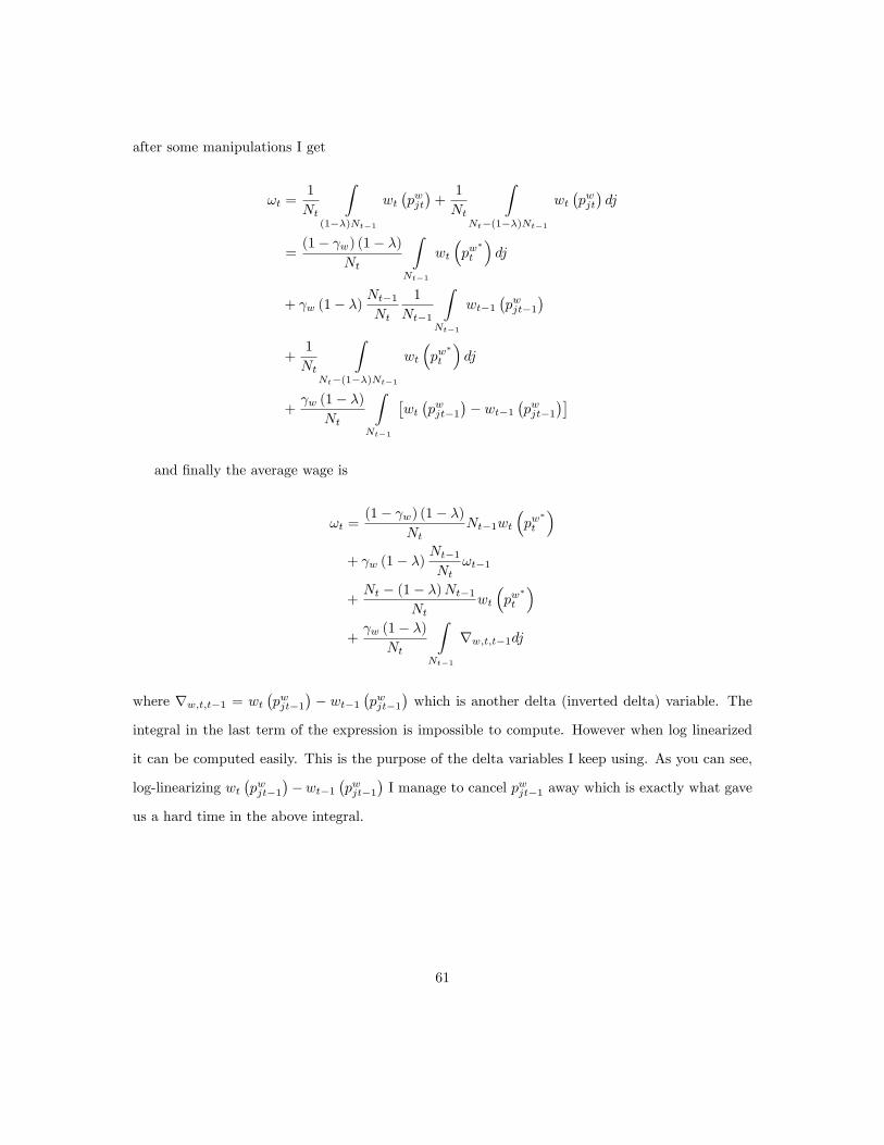
after some manipulations I get

!t =1

Nt

Z(1��)Nt�1

wt�pwjt�+1

Nt

ZNt�(1��)Nt�1

wt�pwjt�dj

=(1� w) (1� �)

Nt

ZNt�1

wt

�pw

�

t

�dj

+ w (1� �)Nt�1Nt

1

Nt�1

ZNt�1

wt�1�pwjt�1

�+1

Nt

ZNt�(1��)Nt�1

wt

�pw

�

t

�dj

+ w (1� �)

Nt

ZNt�1

�wt�pwjt�1

�� wt�1

�pwjt�1

��

and �nally the average wage is

!t =(1� w) (1� �)

NtNt�1wt

�pw

�

t

�+ w (1� �)

Nt�1Nt

!t�1

+Nt � (1� �)Nt�1

Ntwt

�pw

�

t

�+ w (1� �)

Nt

ZNt�1

rw;t;t�1dj

where rw;t;t�1 = wt�pwjt�1

�� wt�1

�pwjt�1

�which is another delta (inverted delta) variable. The

integral in the last term of the expression is impossible to compute. However when log linearized

it can be computed easily. This is the purpose of the delta variables I keep using. As you can see,

log-linearizing wt�pwjt�1

��wt�1

�pwjt�1

�I manage to cancel pwjt�1 away which is exactly what gave

us a hard time in the above integral.

61

Log-linearizing the average wage equation I get the equation for the average economy-wide wage

!t = (1� �) (nt�1 � nt + w�t )� w (1� �) (nt�1 � nt + w�t )

+ w (1� �) (nt�1 � nt + !t�1)

+ w�t � (1� �) (nt�1 � nt + w�t )

+ w (1� �)

�wrt;t�1

The only thing needs to be de�ned is rw;t;t�1. I repeat below the wage equation for a �rm charging

a price pwjt�1 on period t� 1

wt�1�pwjt�1

�=

1

Lt�1�pwjt�1

�264 (1� �)Dt�1

�pwjt�1

�+ (1� �) b

� (1� �)Dut�1 + �Kt�1#t�1 + �

pwjt�1Pt�1

xt�1�pwjt�1

�375

and the wage this same �rm would pay if it failed to adjust its price next period. (Still there is

in�ation indexation in this case)

wt

�pwjt�1

Pwt�1Pwt�2

�=

1

Lt

�pwjt�1

Pwt�1Pwt�2

�264 (1� �)Dt

�pwjt�1

Pwt�1Pwt�2

�+ (1� �) b

� (1� �)Dut + �Kt#t + �

pwjt�1Pt

Pwt�1Pwt�2

xt

�pwjt�1

Pwt�1Pwt�2

�375

where in both equations Dt =G(Lt)�t

is the disutility from labor and Dut =

Gu(Lut )�t

is the disutility

from search e¤ort.

Log linearizing both expressions and subtract I get

rw;t;t�1 = � �w��w � 1�

�At � At�1

�+�w�

��wt � �wt�1

�+1

�

�Xt � Xt�1

��

1�L

266664(1� �) �L1+`��

h�w�1�

�At � At�1

�+ �w

�

��wt � �wt�1

�+ 1

�

�Xt � Xt�1

�� 1

1+` (�t � �t�1)i

� (1� �) �Du�Dut � Du

t�1

�+ � �K �#

�Kt � Kt�1 + #t � #t�1

�+� �P x

�X�N

hP xt � P xt�1 + (�w � 1)

�At � At�1

�+ (�w � 1)

��wt � �wt�1

�+ Xt � Xt�1

i377775

62

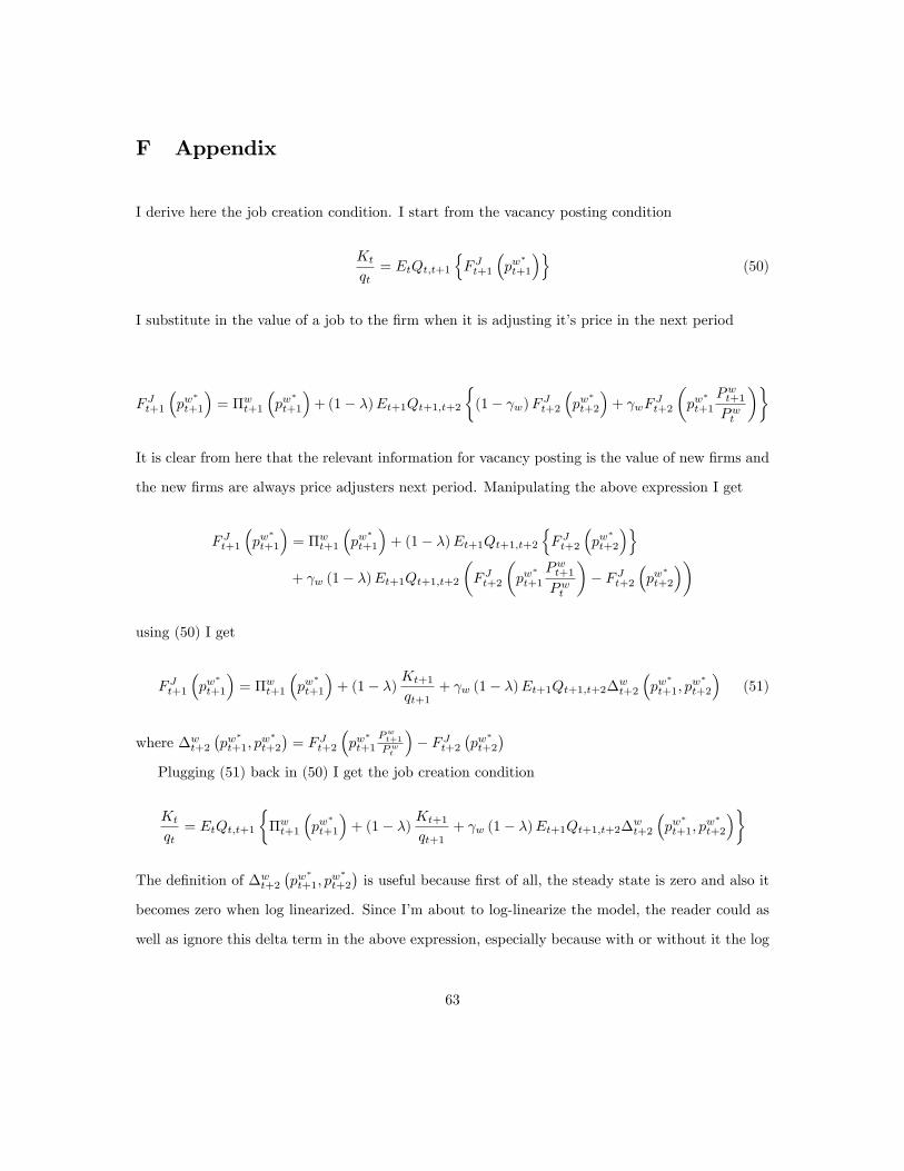
F Appendix

I derive here the job creation condition. I start from the vacancy posting condition

Kt

qt= EtQt;t+1

nF Jt+1

�pw

�

t+1

�o(50)

I substitute in the value of a job to the �rm when it is adjusting it�s price in the next period

F Jt+1

�pw

�

t+1

�= �wt+1

�pw

�

t+1

�+ (1� �)Et+1Qt+1;t+2

�(1� w)F Jt+2

�pw

�

t+2

�+ wF

Jt+2

�pw

�

t+1

Pwt+1Pwt

��

It is clear from here that the relevant information for vacancy posting is the value of new �rms and

the new �rms are always price adjusters next period. Manipulating the above expression I get

F Jt+1

�pw

�

t+1

�= �wt+1

�pw

�

t+1

�+ (1� �)Et+1Qt+1;t+2

nF Jt+2

�pw

�

t+2

�o+ w (1� �)Et+1Qt+1;t+2

�F Jt+2

�pw

�

t+1

Pwt+1Pwt

�� F Jt+2

�pw

�

t+2

��

using (50) I get

F Jt+1

�pw

�

t+1

�= �wt+1

�pw

�

t+1

�+ (1� �) Kt+1

qt+1+ w (1� �)Et+1Qt+1;t+2�wt+2

�pw

�

t+1; pw�

t+2

�(51)

where �wt+2�pw

�

t+1; pw�

t+2

�= F Jt+2

�pw

�

t+1Pwt+1

Pwt

�� F Jt+2

�pw

�

t+2

�Plugging (51) back in (50) I get the job creation condition

Kt

qt= EtQt;t+1

��wt+1

�pw

�

t+1

�+ (1� �) Kt+1

qt+1+ w (1� �)Et+1Qt+1;t+2�wt+2

�pw

�

t+1; pw�

t+2

��

The de�nition of �wt+2�pw

�

t+1; pw�

t+2

�is useful because �rst of all, the steady state is zero and also it

becomes zero when log linearized. Since I�m about to log-linearize the model, the reader could as

well as ignore this delta term in the above expression, especially because with or without it the log

63

linearized expressions will be exactly the same.

G Appendix

In this section I present the details of the structural VAR in �gure 1. The Central Bank sets it�s

instrument it every period given the information available. Therefore the Taylor rule the Central

Bank uses is the following:

it = z (It) + "mt

where it is the nominal interest rate, It the information set at period t , z (:) is a linear function

and "mt is the monetary policy shock. To be able to identify the e¤ect of the monetary policy shock,

I de�ne the following structural VAR:

yt = �+ �t+�1yt�1 +�2yt�2 + :::+�pyt�p +B"t (52)

E ("t) = 0

E ("t"0t) =

In my example yt is a (8� 1), A is a (8� 8) matrix of constants, c and � are (8� 1) coe¢ cients

for the constant and time trend t, �p is the (8� 8) matrix of VAR coe¢ cients for p = 1; ::; 4 and

"t is the (8� 1) vector of shocks with the monetary shock "mt as the last element of this vector. I

use the usual short run restrictions in order to identify the monetary policy shock. I assume that a

policy shock only a¤ects the nominal interest rate contemporaneously. This means that monetary

policy shock a¤ects all variables other than the policy instrument after one period lag. In terms of

the VAR above, this means that the B matrix is lower triangular with unit diagonal elements.

64

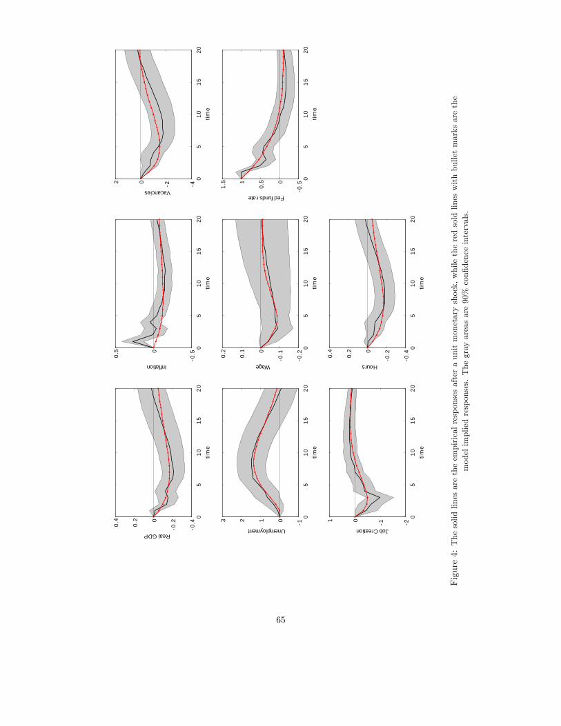
05

1015

20­0

.4

­0.20

0.2

0.4

time

Real GDP0

510

1520

­0.50

0.5

time

Inflation

05

1015

20­4­202

time

Vacancies

05

1015

20­10123

time

Unemployment

05

1015

20­0

.2

­0.10

0.1

0.2

time

Wage

05

1015

20­0

.50

0.51

1.5

time

Fed funds rate

05

1015

20­2­101

time

Job Creation

05

1015

20­0

.4

­0.20

0.2

0.4

time

Hours

Figure4:Thesolidlinesaretheempiricalresponsesafteraunitmonetaryshock,whiletheredsoldlineswithbulletmarksarethe

modelimpliedresponses.Thegrayareasare90%con�denceintervals.

65

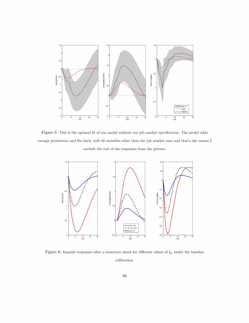
0 5 10 15 20­3

­2.5

­2

­1.5

­1

­0.5

0

0.5

1

1.5

time

Vaca

ncie

s

0 5 10 15 20­1

­0.5

0

0.5

1

1.5

2

2.5

time

Une

mpl

oym

ent

0 5 10 15 20­2

­1.5

­1

­0.5

0

0.5

time

Job 

Cre

atio

n

90% CImodelempirical

Figure 5: This is the optimal �t of our model without our job market speci�cation. The model adds

enough persistence and �ts fairly well all variables other than the job market ones and that�s the reason I

exclude the rest of the responses from the picture.

0 5 10 15 20­2

­1.5

­1

­0.5

0

0.5

time

Vaca

ncie

s

0 5 10 15 20­0.5

0

0.5

1

1.5

2

time

Une

mpl

oym

ent

ξu = 0.3ξu = 0.23ξu = 0

0 5 10 15 20­0.6

­0.5

­0.4

­0.3

­0.2

­0.1

0

0.1

0.2

time

Job 

Cre

atio

n

Figure 6: Impulse responses after a monetary shock for di¤erent values of �u under the baseline

calibration.

66

0 5 10 15 20­1.2

­1

­0.8

­0.6

­0.4

­0.2

0

0.2

0.4

time

Vaca

ncie

s

0 5 10 15 20­0.4

­0.2

0

0.2

0.4

0.6

0.8

1

time

Une

mpl

oym

ent

0 5 10 15 20­0.4

­0.3

­0.2

­0.1

0

0.1

0.2

0.3

time

Job 

Cre

atio

n

φ = 0φ = 1.5φ = 3

Figure 7: I assume a constant disutility of e¤ort (�u = 0) and let the application units � vary.

0 5 10 15 20­3

­2.5

­2

­1.5

­1

­0.5

0

0.5

1

1.5

time

Vaca

ncie

s

0 5 10 15 20­1

­0.5

0

0.5

1

1.5

2

2.5

time

Une

mpl

oym

ent

0 5 10 15 20­2

­1.5

­1

­0.5

0

0.5

time

Job 

Cre

atio

n

90% CImodelempirical

Figure 8: This �gure presents the optimal �t of the model when �u = 0 with a non-zero �. I focus on the

labor market variables again since the rest of the responses perform fairly well.

67

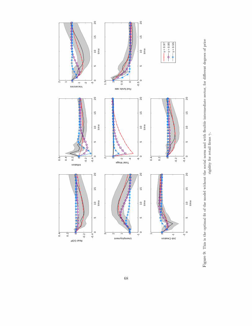
05

1015

20­0

.4

­0.20

0.2

0.4

time

Real GDP

05

1015

20­0

.4

­0.20

0.2

0.4

0.6

time

Inflation

05

1015

20­3­2­1012

time

Vacancies

05

1015

20­10123

time

Unemployment

05

1015

20­6­4­202

time

Total Wage

05

1015

20­0

.50

0.51

1.5

time

Fed funds rate

05

1015

20­2­101

time

Job Creation

05

1015

20­0

.4

­0.20

0.2

0.4

γ = 

0.97

γ = 

0.85

γ = 

0.55

Figure9:Thisistheoptimal�tofthemodelwithoutthesocialnorm

andwith�exibleintermediatesector,fordi¤erentdegreesofprice

rigidityforretail�rms .

68

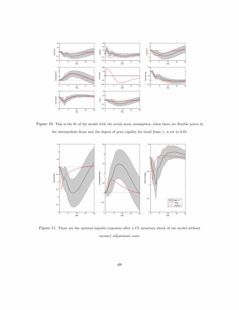
0 5 10 15 20­0.4

­0.2

0

0.2

0.4

time

Rea

l GD

P

0 5 10 15 20­0.4

­0.2

0

0.2

0.4

0.6

time

Infla

tion

0 5 10 15 20­3

­2

­1

0

1

2

time

Vac

anci

es

0 5 10 15 20­1

0

1

2

3

time

Une

mpl

oym

ent

0 5 10 15 20­100

­50

0

50

100

time

Tota

l Wag

e

0 5 10 15 20­0.5

0

0.5

1

1.5

time

Fed 

fund

s ra

te

0 5 10 15 20­2

­1

0

1

time

Job 

Cre

atio

n

0 5 10 15 20­0.4

­0.2

0

0.2

0.4

time

Hou

rs

Figure 10: This is the �t of the model with the social norm assumption, when there are �exible prices in

the intermediate �rms and the degree of price rigidity for retail �rms , is set to 0.85.

0 5 10 15 20­3

­2.5

­2

­1.5

­1

­0.5

0

0.5

1

1.5

time

Vaca

ncie

s

0 5 10 15 20­1

­0.5

0

0.5

1

1.5

2

2.5

time

Une

mpl

oym

ent

0 5 10 15 20­2

­1.5

­1

­0.5

0

0.5

time

Job 

Cre

atio

n

90% CImodelempirical

Figure 11: Those are the optimal impulse responses after a 1% monetary shock of our model without

vacancy adjustment costs.

69

R&D, Product Innovation and Employment

10 December 2010

Abstract

In this study I attempt to solve the ampli�cation puzzle, the inability of the standard search

and matching model to account for the volatility in vacancies and unemployment, by exploring

the connection between R&D and employment. R&D a¤ects product creation and product

creation a¤ects employment. An improvement in technology bene�ts the economy in two ways.

Same products can be produced more e¢ ciently and also new products are created. Empirical

evidence suggest that the increase in production for already existing goods does not imply

increases in employment, while new products are associated with increases in employment.

The search and matching model implies that changes in technology do not imply large changes

in employment for already existing goods which is in line with what the evidence suggest.

However, when the search and matching model applies for sectors that innovate and produce

new products, changes in employment signi�cantly increase. Therefore, in this model I assume

all agents need to innovate �rst before they create a job opening, because �rms that invent

new products are the ones that contribute more to the volatility of employment according to

the evidence. Since ideas are cheaper to implement after a technological expansion, the cost

of vacancies becomes countercyclical which boosts job creation and vacancies. The model can

amplify the volatilities of vacancies, unemployment and market tightness approximately by up

to 300 percent.

70

1 Introduction

The standard search and matching model by Mortensen and Pissarides (1994), despite it�s intuitive

framework and predictions, it cannot replicate the volatility of vacancies, unemployment and market

tightness observed in empirical exercises (Shimer (2005), Fujita (2003)). There are many attempts

to resolve the issue and the solutions proposed insinuate di¤erent implications for policy analysis1 .

I follow a di¤erent route from the literature and attempt to explore how the connection between

investments in R&D and the cost of inventing new products (jobs) can increase the volatilities of

vacancies, unemployment and market tightness.

The importance of Research And Development (R&D) on technology and productivity has been

studied extensively over the past decades especially by growth economists. Although the in�uence

of R&D on productivity is undisputed, the impact of innovation and R&D on employment is

controversial. R&D and innovation can a¤ect productivity through two di¤erent channels, process

innovation and product innovation. Process innovation involves original ways of producing goods

and services while Product innovation involves the creation of new or di¤erentiated products. Even

though authors like Greenan and Guellec (2000), Bogliacino and Pianta (2010) and others �nd

that the e¤ect of process innovation on employment is arguable, they all agree that the e¤ect of

product innovation on employment is positive and statistically signi�cant. That is because process

innovation may destroy jobs since newly invented machines or advances in productivity can deem

some jobs obsolete while product innovation leads to more job openings, by unveiling new economic

channels. Some vacancies can be thought as a by-product of product innovation. Some jobs are

created by �rms that create new products. My argument is that those particular �rms are the ones

that make vacancies and job creation so volatile in the data. A new job can be considered as a new

�rm or product and a new product is a new idea that needs to be invented which can be put to

production only after it �nds a worker to put the idea to life.

I create a framework where every �rm/job is a di¤erentiated product and product innovation

needs the services of an R&D �rm for the idea to appear and a worker to implement this idea for

1Form more information about the issues and recent attempts you can check Cardullo (2008).

71

production purposes. To open a vacancy you need a new idea for a product. The R&D �rm is

charging a fee for it�s service and this is the only cost to post a vacancy2 . Moreover, R&D �rms

invest in the quality of the ideas they provide and higher quality entails greater e¢ ciency in the

production of ideas for new products. This implies that in an expansion, vacancy demand increase

and investment in R&D rises which makes the cost of producing vacancies lower and even more

vacant positions to be opened.

The reduced cost of ideas a¤ects vacancy creation in two ways. First it lowers vacancy costs

directly and second it extends �rm�s pro�ts by diminishing the wage bargained by the workers.

The two main ingredients for innovative �rms to exist are an idea and a worker. In an expansion,

although workers are harder to �nd and expensive to keep, ideas are easier to be created and

implemented. A job is a combination of an idea and a worker and the degree up to which a �rm

values each element determines it�s bargaining power and the wage it pays it�s worker. However,

when one element becomes more valuable, the other becomes more cheap, balancing the bargaining

power of the �rm, leaving the wage less responsive and pro�ts along with incentives to post vacancies

more volatile. In other words, lower vacancy costs tend to decrease the wage from a job match

because the outside opportunity of the �rm (the vacancy state) becomes more bene�cial whenever

bargain power in the current match slips from the hands of the �rm and vice versa.

The addition of investments in R&D can amplify the volatilities of vacancies, unemployment and

market tightness considerably. The model cannot account for the volatility of the real wage, but

could be considered as part of a more complex model where some kind of wage rigidity is present

to keep the wage from overshooting. The connection of R&D investment and job creation might be

one of the missing links in the search and matching theory that may need to be further explored

by researchers.

The following sections include the following features: The exploration of the connection between

R&D and employment along with some empirical evidence by other authors. A detailed derivation

of the R&D sector that explicitly de�nes the price of a vacancy as a function of aggregate vacancy

2There could be also a cost to advertise the vacancy which is the standard assumption in the search and matchingmodels. Refraining to assume that on top of the cost to come up with the idea to open a vacancy there are advertizingcosts does not change the results of this paper.

72

demand. After the R&D sector is fully de�ned, I present the rest of the model, followed by the

calibration section and the results.

2 The Impact of R&D on Employment

Does innovation and new technology create or destroy jobs? This is a rather di¢ cult question that

has been bothering researchers from classical economists to today. During the �rst industrial revo-

lution, British workers in fear of technological unemployment destroyed the machines in industrial

areas as well as the countryside. Technology can actually destroy a lot of jobs rapidly but can also

create some. Lots of workers have been replaced by machines during the last few decades where

technological progress has become more pervasive. However, technological progress is a rather vague

idea as technological innovation could mean di¤erent things. Technological progress could either

come in the form of process innovation or in the form of product innovation.

Process innovation involves advances in the way of producing certain goods and services. Process

innovation is the form of technological progress that could rapidly shed a large number of jobs in-

stantaneously, at least in the short run. However, economists responded to the critics of technolog-

ical innovation by putting forward a theory that Marx called "compensation theory". The theory

includes di¤erent compensation mechanisms in various markets that can actually counterbalance

the initial shed of jobs due to process innovation. Empirical analysis by various authors such as

Greenan and Guellec (2000), Pianta (2005), Garcia et. al (2002), Evangelista (2000), Blanch�ower

and Burguess (1998) report controversial evidence about the relation between process innovation

and employment.

Product innovation is a form of technological progress that involves the creation of new or

di¤erentiated products. Product innovation can create new economic branches along with new job

positions. It is the most "labor-friendly" form of technological progress. Despite any ambiguity

in the impact of process innovation on employment, there is a consensus that product innovation

stimulates employment as proclaimed by Harrison et al (2005), Peters (2005), Bogliacino and Pianta

(2010), Vivarelli and Pianta (2000), Edquist, Hommen and McKelvey (2001), Freeman and Soete

73

(1994) and others. Moreover, R&D expenditures can boost product innovation which consequently

increase job creation. The direct impact of R&D on employment is investigated by Bogliacino and

Vivarelli (2010).

In this paper I impose a rather strong assumption. I assume that for a job to be created, an idea

of a new product needs to be generated. This is not entirely realistic since some jobs are simply

created along premises that already exist. For example, if I have a secretary and I wish to hire

another one, then there is no need for an idea or research or R&D of any sort to create this job

opening. Not all jobs come from new and innovative products or ideas. Nevertheless, I make this

assumption based on the empirical evidence about the e¤ect of product innovation I have already

discussed. The �uctuations in employment tend to be related to the e¤ect of new product creation.

Therefore, I assume that in the model economy there are only �rms that are innovative. You could

think of this model as a simpli�ed version of a relatively more complicated model, where there are

two types of �rms. Firms that do not innovate and �rms that innovate and produce new goods. The

�rms that create already existing jobs with no need of R&D are going to have the same structure as

the standard search and matching model where the e¤ect of a technology shock on job creation in

that sector would be minimal. The other sector, containing the �rms that are creative to the point

of designing new products, is going to be the one that is going to generate most of the volatility

in employment, which is in line with what the empirical evidence suggest. In my model I discard

completely the �rst sector and just assume that all new jobs produce new and innovative products

since that particular sector is going to be the one that creates the largest employment �uctuations

in the �rst place.

The above authors have a lot of explanations as to why process innovation might not necessarily

be translated to more jobs. My own explanation lies exactly along the lines of the standard search

and matching model�s woes. The search and matching model predicts that after a productivity

shock, job creation and employment are barely responsive. This should not be a problem at all

since process innovation actually does not seem to create new jobs. Even though the e¤ect of a

technology shock raises productivity and output, the e¤ect on employment is rather mild. Product

innovation is the one that is associated with employment �uctuations. The standard search and

74

matching model assumes that increases in productivity lead to a very mild increase in the creation

of more of those same �rms, which is what the empirical evidence suggest. If one is interested to

see after a appositive productivity shock,whether many more of the same jobs/�rms are going to

appear, the search and matching model gives actually the right answer. Not many of the same

jobs will suddenly appear. If we allow new products to be created, the search and matching model

-as I tend to show in this paper- implies that a positive technology shock can amplify job creation

signi�cantly, exactly what those authors predict the connection between product innovation and

technology should be.

Speci�cally, in this paper I assume that an increase in employment can only be achieved through

product innovation. Every �rm is a single job producing a di¤erentiated product. Therefore, for a

�rm to be created, a di¤erentiated product needs to be created and a worker needs to be employed.

I create the necessity for R&D services for agents seeking to create vacancies. I assume vacancies

are potential di¤erentiated products that need to be developed and their development needs ideas.

R&D �rms are in charge of providing ideas for a fee and also invest in the quality of their services.

In a sense, R&D �rms are in charge of product innovation. The higher the quality investment in

R&D, the more e¢ cient those research �rms are in producing ideas or vacancies. Higher quality

research makes ideas �oating from the R&D sector more e¤ective and the fee they charge for each

vacancy lower. In an expansion, vacancies increase and R&D �rms invest more in the quality of

their service. Improved quality enhances R&D �rms�productivity and higher productivity in R&D

makes the cost of vacancies to drop, creating another wave of potential job positions, boosting

overall vacancies and job creation. In other words I create a theoretical framework where vacancies

are considered as ideas of new product along with an opening for a worker to put this idea into

production. I demonstrate that the additional impact of improvements in R&D on employment

is important for job creation and this is something that might have been ignored in the search

and matching literature so far. Product innovation is important for employment and the level of

R&D can boost the capacity of ideas produced. Thus, as suggested by the empirical evidence, the

cyclicality of R&D might be one of the driving forces of the large cyclical variations in employment

that is missing from the standard search and matching model and this is what the purpose of this

75

paper is all about.

3 R&D Firms

Jobs in my model are di¤erentiated products, therefore vacancies are ideas about di¤erentiated

products and the invention of a vacant position needs research. Consumers in the economy are

capable of producing ideas and ideas are the main ingredient for vacancy creation. Consumers are

basically the R&D �rms even though the speci�cation of who provides the ideas is of minor impor-

tance. Therefore there�s a market for ideas and agents attempting to create a �rm through vacancy

creation, need those services. Individual ideas vst can be produced by the following production

function:

vst = (Lvst)

1� (1)

where Lvst is part of the �nal good and vst the number of ideas the sth individual provides. In some

sense this is the amount of food needed to produce ideas. It�s basically food for thought.

The aggregate research service or vacancies produced Vt in this sector is a combination of all

the ideas in the economy, where qst is the quality of the sth researcher

Vt =

24 1Z0

�q�stvst

� �v�1�v ds

35�v

�v�1

The cost minimization problem of the agent that purchases this aggregate research good in an

attempt to create vacancies implies that the demand for ideas for the individual R&D �rm is:

vst = q�(�v�1)st

�pvstP vt

���vVt (2)

where pvst is the price the individual R&D �rm charges for it�s services. Also from the same cost

76

minimization problem the price of the aggregate vacancies posted is:

P vt =

24 1Z0

�pvstq�st

�1��vds

351

1��v

which states that the aggregate price is the aggregate of the individual quality adjusted prices.

Since all agents provide the same amount of ideas the above relative price becomes:

pvstP vt

= q�st (3)

and the demand (2) can be written alternatively as

vst = q�(��1)st (qst)

���Vt =

Vtq�st

(4)

The pro�t maximization problem of the individual R&D �rm which decides the price and in-

vestment in research quality is:

maxfpvt ;qtg

E0Xt=0

Q0;t

�pvtPtvt �

PtPtLvt � c (qt)

�

where c (qt) is the cost of employing quality qt and Q0;t stochastic discount factor.

s.t.

the demand for

vt = q�(�v�1)t

�pvtP vt

���vVt

the idea production function

v�t = Lvt

I drop the s subscript because every individual is identical and the decision problem is the same

77

for all R&D �rms. Substitute the constraints into the objective to get

maxfpvt ;qtg

E0Xt=0

Q0;t

8<:pvtPt q�(�v�1)t

�pvtP vt

���vVt �

"q�(�v�1)t

�pvtP vt

���vVt

#�� c (qt)

9=;The F.O.C with respect to pvt is

pvtPt=

��v�v � 1

"q�(�v�1)t

�pvtP vt

���vVt

#��1(5)

Use the fact that every research �rm charges the same price, equation (3) and the relative price of

an individual�s ideas is:pvtPt=

��v�v � 1

�Vtq�st

���1(6)

This means that the relative price of vacancies P xt is

P xt �P vtPt

=��v

(�v � 1)1

q�t

�Vtq�st

���1(7)

The F.O.C with respect to qt is

� (�v � 1)

24pvtPt� �

q�(�v�1)t

�pvtP vt

���vVt

!��135 q�(�v�1)�1t

�pvtP vt

���vVt = c

0 (qt) (8)

and after using (3), (5) and (6)

��

�Vtq�t

���1q�(1+�)�(1��)t V �t = c

0 (qt) (9)

3.1 The Vacancy Cost

Start from the cost of vacancies as a function of both the aggregate vacancy number Vt and quality

qt, equation (7), which is repeated below

P xt �P vtPt

=1

qt

��v(�v � 1)

�Vtqt

���1

78

If � < 1, it means the production of ideas exhibits increasing returns to scale and therefore the

cost of a vacancy would be decreasing without the need of quality to play any particular role. The

negative relation between vacancies and its cost can be guaranteed by the increasing returns to

scale assumption. I do not intent to assume increasing returns to scale thus I set � = 1. My goal

in this section is to eliminate qt in the above equation to derive an expression between the cost of

vacancies and the aggregate demand for vacancies in the economy.

In order to be able to observe what the introduction of quality in R&D can imply for vacancy

dynamics, assume c0 (qt) = c. Use the �rst order condition for quality, equation (9). Solve for qt

and get

qt =� c�

� 11+�

V1

1+�

t (10)

Then eliminate qt from the expression for the cost of a vacancy, equation (7). That is

P xt =��v

(�v � 1)

��

c

� �1+�

V� �1+�

t

The cost of vacancies is a constant times a function of vacancies

P xt = �V� �1+�

t (11)

where � = ��v(�v�1)

��c

� �1+� is that constant. Equation (11) summarizes the result of the paper and I

am going to refer to it immediately after I restate the puzzle and my goal in the next section.

3.2 Puzzle and Solution

The ampli�cation puzzle arises in the search and matching model due to the wage implied by the

speci�c bargaining problem faced by both �rms and workers according to this framework. The

problem is that the wage is too dependent on the value of workers� outside opportunity which

is unemployment. After an expansionary productivity shock, vacancies rise and unemployment

drops. The few unemployed are facing a large number of available jobs which gives employed

workers bargaining power. The employed worker can reach for a higher wage by threatening to

79

break the current match now that the unemployment duration has dropped signi�cantly. The �rm

is in a bad position to negotiate because if the match breaks, the average duration of a vacancy

is relatively high compared to unemployment duration. Therefore the worker can negotiate such

a high wage that basically diminishes �rm�s pro�ts and the incentive to post vacancies to begin

with. In the standard search and matching model, the wage absorbs most of the e¤ect of the shock

leaving pro�ts and consequently vacancies barely responsive.

However, this is the e¤ect of a technology shock on vacancies and employment if more of the

already existing jobs are created. The story is di¤erent for �rms that innovate. Even before I

present the whole model, the main result can be observed simply by looking equation (11) that I

repeat below

P xt = �V� �1+�

t

This equation states that the cost of a vacancy is decreasing in the number of vacancies demanded.

The above relationship arises due to quality improvements by the research �rms. The greater the

vacancy demand, the larger the pro�t the R&D �rm experiences and thus the larger the capability

of investment in the quality of the �rm�s product. The quality improvement increases productivity

and enables the R&D �rm to further decrease it�s cost.

After a positive technology shock, the cost of a vacancy drops according to the equation above

which can boost job creation and vacancies through two channels. The �rst channel is the obvious

one. Lower cost of vacancies means more vacancies posted. However there is another channel

that is not as obvious. Lower cost of a vacancy a¤ects the relative bargaining power between �nal

good �rms and workers. In an expansion the duration of a vacancy increases, but the cost of a

vacancy drops since R&D �rms can improve their quality. Lower vacancy cost puts �rms back into

the negotiations game. It enables the �rm to deny a too high wage to the worker since upon a

destruction of a match, the �rm is not in a bad situation anymore. The average vacancy duration

may be large in a boom but according to (11) the vacancy cost decreases improving �rms�outside

opportunities which is the value of the vacancy state. This prevents the wage from absorbing most

of the e¤ect of the shock as in the standard search and matching model, thus boosting pro�ts and

80

Figure 1: The agents in the model, their basic interactions and the �ow of goods and services.

the incentive to post even more vacancies.

A job has two elements when only the innovative �rms are considered. The �rst element is

an original idea and the second a worker to put this idea into the production process. Along the

business cycle the scarcity of those elements varies. Novertheless, it varies in such a way that when

workers are more scarce, ideas are more wasy to grasp or impliment and vice versa, meaning that

the �rm does is not facing a wage that absorbes most of the e¤ect of the shock anymore.

Therefore, innovative �rms face a quite di¤erent bargaining problem than usual �rms and this is

the main reason that the search and matching model fails to explain the ampli�cation puzzle. How-

ever, the standard model actually predicts that advances in technology may enhance productivity

or output but not employment as much simply because all �rms in the standard model produce

the same product. When �rms that create new products are examined, the wage structure implied

from the search and matching model does not hinder job creation to expand.

81

4 The Model

The model consists of three agents as can be seen in �gure 1. Households that choose consumption

every period and also post vacancies which when successfully matched can become a �rm with the

household as the only shareholder. Vacancies are new products or jobs and their creation needs

the services of creative minds. R&D �rms provide those ideas to households trying to open job

positions in exchange for a fee. Moreover households provide labor to the �nal good �rms which

use it as an input. The number of employed workers, hours and wages are determined as in the

traditional search and matching model. Final good �rms use labor to produce the �nal good which

is partly consumed by the households and the rest is used as an input by R&D �rms for the creation

of ideas for product (or job) innovation.

4.1 Household Problem

There is a large number of identical households each containing Ih members. Therefore all house-

holds are identical supporting market completeness as in Merz (1995). A measure of Nwht household

members are employed while the rest Ih � Nwht remains unemployed. Households get utility from

consumption and disutility from labor. In addition, households post vacancies in an attempt to

gain ownership of �nal good �rms. Every consumer in the economy employed or not is able to

produce ideas that are a necessary ingredient for job creation. There are many households each

maximizing the following utility function:

U (Cht; Lhjt) =(Cht � �Ct�1)1��

1� � �ZNwht

(Lhjt)1+`

1 + `dj

82

subject to:

Cht +Bht + Pxt Vht

= (Ih �Nwht) bt +

ZNwht

whjtLhjtdj + Tht

+

ZNht

�itdi+ sht

1Z0

�vhstds+ (1 + it�1)Bht�1

Nht+1 = (1� �)Nht + gtVht

where Cht is the consumption chosen by the household h, Ct�1 the aggregate consumption, Lhjt

the labor hours in production from the Nwht employed workers and L

vhkt the e¤ort chosen in the

production of ideas from each of the Ih members of the household. Real Bond holdings is Bht, P xt the

price R&D �rms charge per vacancy and Vht the vacancies the household posts. The unemployment

bene�t received by the household�s unemployed Ih�Nwht is bt. The household receives whjtLhjt wage

income from the Nwht employed workers. The household earns dividends from consumption good

�rms �it and research �rms �vhst, the �rms providing the "ideas". The number of �rms owned

by the household Nht+1 next period is the surviving �rms from the previous period (1� �)Nht

(�rms are destroyed with probability �) plus the vacancies the household posts Vht weighted by the

probability of a vacancy to match gt.

The �rst order conditions for bonds give:

1

1 + it= �Et

�ht+1�ht

where �ht is marginal utility.

The �rst order condition for vacancies implies

P xtgt= EtQt;t+1�t+1 + (1� �)EtQt;t+1

P xt+1gt+1

83

Moreover, in equilibrium the equation of the evolution of the economy-wide employment is

Nt+1 = (1� �)Nt +Mt (12)

where

Mt = mV1��t (1�Nt)�

is the constant returns to scale matching function.

4.2 The Bellman Equations

4.2.1 The �rms

The value of a vacancy to the �rm is:

FVt = �P xt + gtEtQt;t+1F Jt+1 + (1� gt)EtQt;t+1FVt+1 (13)

where P xt is the cost of a vacancy. Next period the vacancy becomes a job with value FJt+1

weighted by the probability of a vacancy to be matched gt or it remains a vacancy with probability

1�gt. Since the value of a vacancy is zero due to free entry, then the above condition in equilibrium

becomesP xtgt= EtQt;t+1F

Jt+1

The value of a job to the �rm is:

F Jt = �t + (1� �)EtQt;t+1F Jt+1 (14)

where �t is the pro�t of the �nal good �rm which survives the next period with probability 1��.

Since the value of a vacancy is zero, then (13) becomes:

P xtgt= EtQt;t+1F

Jt+1

84

and after using (14) we get the job creation condition which can also arise from the household

maximization problem with respect to Vht

P xtgt= EtQt;t+1�t+1 + (1� �)EtQt;t+1

P xt+1gt+1

(15)

4.2.2 The workers

The value of a job to the worker is:

WEt = wtLt �

G (Lt)

�t+ EtQt;t+1

�(1� �)WE

t+1 + �WUt+1

�(16)

where wtLt is the wage received and G (Lt) is the disutility of labor in utility units and �t the

marginal utility. Next period the job is either continued or terminated with probabilities 1�� and

� respectively.

The value of unemployment to the worker is:

WUt = bt + EtQt;t+1

��tW

Et+1 + (1� �t)WU

t+1

�(17)

where bt is the unemployment bene�t and �t the probability corresponding to the event of a worker

to �nd a job.

4.2.3 Bargaining and wage

Firms maximize the surplus from a match by choosing the price. The total surplus is the sum of

the surpluses a successful match generates.

St = FJt � FVt +WE

t �WUt

Firms and workers engage into Nash bargaining and split the surplus by assigning � share to the

workers and the rest 1� � to the �rms. The above procedure is similar to maximizing the objective

85

below with respect to the wage.

maxwt

n�F Jt � FVt

�1�� �WEt �WU

t

��o

The �rst order condition results to:

(1� �)�WEt �WU

t

�= �

�F Jt � FVt

�Substitute in the above the the value of a job to the �rm equation (14), the value of a job to

the workers equation (16) and the value of unemployment equation (17). This implies the wage

equation is

wtLt = (1� �)�G (Lt)

�t+ bt

�+ �P xt #t + �

ptPtyt (18)

= (1� �)

1

1 + `

L1+`t

�t+ bt

!+ �P xt #t + �

YtNt

There are Nt employed individuals or equivalently, there are Nt �nal good �rms. Each �rm uses

Ljt units of the worker�s e¤ort as input to produce the di¤erentiated good yjt via the following

production function

yjt = ZtLjt (19)

where Zt is an AR(1) productivity shock following

Zt = (1� �z) + �zZt�1 + "t

and "t is iid. The aggregate consumption good is a combination of all individual �rms�outputs.

The aggregation is according to the following Dixit-Stiglitz function

Yt = At

24ZNt

y��1�

jt dj

35 ���1

86

where

At � N�� 1

��1t

and � is the Love Of Variety parameter. The aggregate price of the composite good Yt is

Pt =1

At

24ZNt

p1��

jt dj

35 11��

(20)

and the demand for each good yjt which is used mainly for consumption is:

yjt = A��1t

�pjtPt

���Yt (21)

The �rms maximize the total surplus from a match by choosing every period the price they

charge for their good. The total surplus to be maximized is

St = FJt � FVt +WE

t �WUt (22)

From the Bellman equations of the precious section substitute the �rm�s and worker�s surpluses in

the above for the total surplus, to �nd the surplus as a function of pjt the price the �rm charges

for its services. Moreover, use the fact that the pro�t is �jt =pjtPtyjt � wtLt. After the above

manipulations, maximizing the total surplus is equivalent to maximizing the following objective

function:

maxpt

�pjtPtyjt �tLt

�subject to the demand function (21), and the production function (19). The function t =

G(Lt)�t

is the disutility from providing Lt labor e¤ort in terms of the real good. The �rm maximizes the

surplus by treating t as �xed. For further details on this result check Koursaros (2009).

The �rst order condition implies the usual monopoly result that the price is a markup over the

real marginal cost. Ignore the j subscript since all �rms are identical. The relative price of a single

87

�rm then should beptPt=

�

� � 1tZt

Final good �rms should set the relative price equal to the marginal cost which is the disutility of

laborptPt=

�

� � 1LtZt

and substitute the expression for the disutility of labor G (Lt) = L`t to get

ptPt=

�

� � 1GL (Lt)

�tZt

and since ptPt= N �

t I get

N �t =

�

� � 1L`t�t

1

Zt

L1+`t

�t=� � 1�

YtNt

Plug this into the wage equation (18) to get

wtLt = (1� �)�

1

1 + `

� � 1�

YtNt+ bt

�+ �P xt #t + �

YtNt

In a similar fashion the pro�t of the �rm after substituting in the wage equation above is:

�t =ptPtyt � wtLt

= (1� �) 1 + `�

� (1 + `)

YtNt� (1� �) bt � �P xt #t

Keep in mind that the pro�t of the �rm which appears in the job creation condition (15) and the

objective of the �rm are not the same. The �rm maximizes the surplus and not the pro�t. The

pro�t is part of the surplus. However, investors care about cash �ows and not the surplus, therefore,

the job creation condition is a statement about cash �ows.

88

4.2.4 The solution

The following system characterizes the solution:

The feasibility constraint:

Yt = Ct + Pxt Vt (23)

where I assume the vacancy costs are subsidized by the government.

The law of motion of employment:

Nt+1 = (1� �)Nt + h (Vt)� (1�Nt)1�� (24)

The job creation condition:

P xtgt= EtQt;t+1�t+1 + (1� �)EtQt;t+1

P xt+1gt+1

(25)

The pro�t of the �rm producing the consumption good:

�t = (1� �)1 + `�

� (1 + `)

YtNt� (1� �) bt � �P xt #t (26)

The pro�t maximizing condition of the �rm producing the consumption good

N`(1+�)+�t Z1+`t =

�

� � 1Y `t�t

(27)

The cost of a vacancy (cost of producing ideas)

P xt =�v

(�v � 1)

��

c

� �1+�

V� �1+�

t (28)

and the condition for the evolution of quality

qt =� c�

� 11+�

V1

1+�

t (29)

89

Equations (23) to (29) characterize the solution.

4.2.5 The price of ideas and vacancy dynamics

It is easy now to show the mechanism that can boost job creation by examining the appropriate

equations as I have already presented all the equations governing the dynamics in the model. Solve

forward the job creation condition (15)

P xtgt= Et

1Xj=0

(1� �)j Qt;t+j+1�t+j+1 (30)

The above equation states that in equilibrium the cost of a vacancy is P xt (the per unit of time

cost) times the duration of a vacancy 1gt. The cost should be equal to the present discounted value

of all future pro�ts the job is expected to produce for as long it is expected to survive. During an

expansion, jobs are created and vacancies rise. However according to (11) the cost of a vacancy

diminishes since the cost is decreasing in vacancies due to investments in quality that boosts research

productivity. Therefore the �rst channel is through lowering the left hand side of the job creation

condition which represents the cost of a vacancy.

The second channel in which the cost of a vacancy P xt a¤ects job creation is through pro�ts �t

in the above equation and speci�cally through the wage. Remember the wage is part of the �rm�s

pro�t and is determined by:

wtLt = (1� �)�

1

1 + `

� � 1�

YtNt+ bt

�+ �P xt #t + �

YtNt

The cost of a vacancy P xt a¤ects the bargaining power of �rms, thus lower Pxt grants more negoti-

ating power to the �rms because the �rm can �nd another worker less costly. Therefore, during an

expansion, vacancies are created and the increase in vacancies induces a decrease in prices through

improvements in quality. The decrease in the cost of a vacancy boosts vacancies through lower costs

(left hand side of (30)) and through higher pro�ts (right hand side of (30)). The latter comes from

the dependence of the wages on outside factors such as the cost of a vacancy. During a bargaining

90

with the worker, the �rm has the option to leave the bargaining stage and keep the job vacant.

The cost of the vacancy is the �rm�s outside option and lower costs give bargaining power to �rms

and eventually lead to a lower wage for the worker. The lower wage increases �rm�s pro�ts and

investors incentives to open vacancies.

The story so far might have created a logical paradox. I assumed the cost of a vacancy involves

the cost of producing ideas. The reader might be wondering how does that enter the wage equation.

In the wage equation, the cost of a vacancy enters as an outside option for the �rm in the case the

match is destroyed. If a match is destroyed, the ideas still exists. Why would the �rms need to

recreate an idea if a match is destroyed? I assume that upon destruction �rms and ideas disappear.

This might not be entirely realistic but if one thinks about the cost of �rm and job destruction,

it certainly involves the destruction of ideas, capital and human capital, stocks that need some

di¤erentiation to be able to reused in the production process again.

5 Calibration and results

In the following sections I calibrate the model to common parameter values either from estimates

from US data or values obtained by other macroeconomic studies. I simulate the model in order to

provide second moments for the volatilities of vacancies, unemployment, tightness, output, wages,

hours and quality in R&D. The volatilities implied by the model are compared to the ones from

quarterly US data from 1955-2005.

The variables in the US data are basically: the log of quarterly real GDP, the annualized

quarterly rate of change in the CPI, the log of Help-Wanted advertising, the civilian unemployment

rate, the log of job creation for continuing establishments in the manufacturing sector, the log of

average hourly earnings in the business sector, the log of total hours in the business sector and the

e¤ective federal funds rate.

91

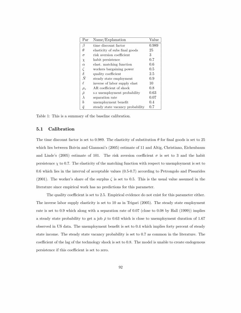
Par Name/Explanation Value

� time discount factor 0:989� elasticity of subs �nal goods 25� risk aversion coe¢ cient 3� habit persistence 0:7� elast. matching function 0:6� workers bargaining power 0:5� quality coe¢ cient 2:5�N steady state employment 0:9` inverse of labor supply elast 10�z AR coe¢ cient of shock 0:8�� s.s unemployment probability 0:63� separation rate 0:07b unemployment bene�t 0:4�q steady state vacancy probability 0:7

Table 1: This is a summary of the baseline calibration.

5.1 Calibration

The time discount factor is set to 0:989. The elasticity of substitution � for �nal goods is set to 25

which lies between Boivin and Giannoni�s (2005) estimate of 11 and Altig, Christiano, Eichenbaum

and Linde�s (2005) estimate of 101. The risk aversion coe¢ cient � is set to 3 and the habit

persistence � to 0.7. The elasticity of the matching function with respect to unemployment is set to

0.6 which lies in the interval of acceptable values (0.5-0.7) according to Petrongolo and Pissarides

(2001). The worker�s share of the surplus � is set to 0.5. This is the usual value assumed in the

literature since empirical work has no predictions for this parameter.

The quality coe¢ cient is set to 2.5. Empirical evidence do not exist for this parameter either.

The inverse labor supply elasticity is set to 10 as in Trigari (2005). The steady state employment

rate is set to 0.9 which along with a separation rate of 0.07 (close to 0.08 by Hall (1999)) implies

a steady state probability to get a job �� to 0.63 which is close to unemployment duration of 1.67

observed in US data. The unemployment bene�t is set to 0.4 which implies forty percent of steady

state income. The steady state vacancy probability is set to 0.7 as common in the literature. The

coe¢ cient of the lag of the technology shock is set to 0.8. The model is unable to create endogenous

persistence if this coe¢ cient is set to zero.

92

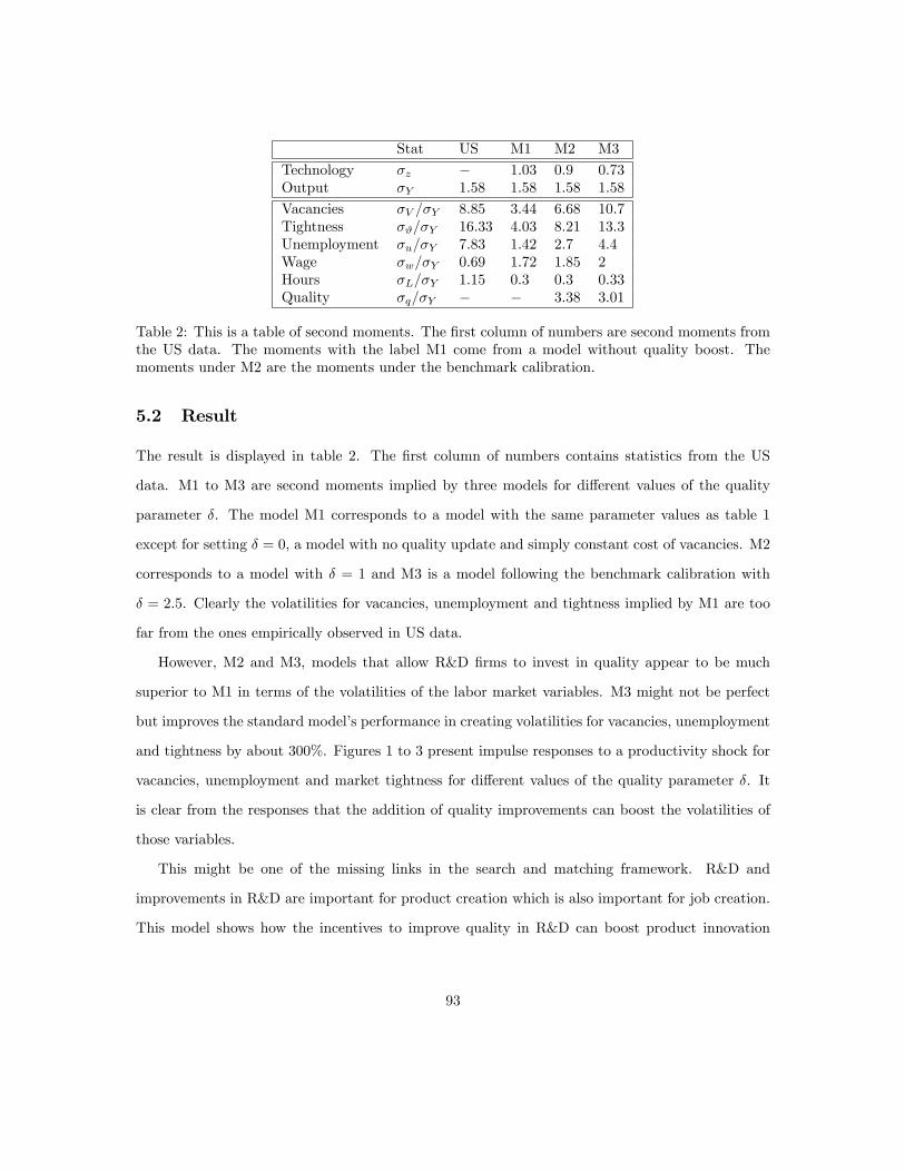
Stat US M1 M2 M3

Technology �z � 1:03 0:9 0:73Output �Y 1:58 1:58 1:58 1:58

Vacancies �V =�Y 8:85 3:44 6:68 10:7Tightness �#=�Y 16:33 4:03 8:21 13:3Unemployment �u=�Y 7:83 1:42 2:7 4:4Wage �w=�Y 0:69 1:72 1:85 2Hours �L=�Y 1:15 0:3 0:3 0:33Quality �q=�Y � � 3:38 3:01

Table 2: This is a table of second moments. The �rst column of numbers are second moments fromthe US data. The moments with the label M1 come from a model without quality boost. Themoments under M2 are the moments under the benchmark calibration.

5.2 Result

The result is displayed in table 2. The �rst column of numbers contains statistics from the US

data. M1 to M3 are second moments implied by three models for di¤erent values of the quality

parameter �. The model M1 corresponds to a model with the same parameter values as table 1

except for setting � = 0, a model with no quality update and simply constant cost of vacancies. M2

corresponds to a model with � = 1 and M3 is a model following the benchmark calibration with

� = 2:5. Clearly the volatilities for vacancies, unemployment and tightness implied by M1 are too

far from the ones empirically observed in US data.

However, M2 and M3, models that allow R&D �rms to invest in quality appear to be much

superior to M1 in terms of the volatilities of the labor market variables. M3 might not be perfect

but improves the standard model�s performance in creating volatilities for vacancies, unemployment

and tightness by about 300%. Figures 1 to 3 present impulse responses to a productivity shock for

vacancies, unemployment and market tightness for di¤erent values of the quality parameter �. It

is clear from the responses that the addition of quality improvements can boost the volatilities of

those variables.

This might be one of the missing links in the search and matching framework. R&D and

improvements in R&D are important for product creation which is also important for job creation.

This model shows how the incentives to improve quality in R&D can boost product innovation

93

which implies increases in employment as the empirical evidence also suggest.

All three models overshoot the wage volatility. Wage rigidity could �x this issue even though

wage rigidity should be imposed only on existing �rms to be consistent with evidence by Pissarides

(2007) and Haefke Sonntag and van Rens (2007). In the current paper I do not propose a mechanism

to account for the volatility of the real wage, however wage rigidity for ongoing �rms can be the

best candidate.

Employment is not as volatile and makes tightness not as volatile as it could be. The reason

is the equation for the evolution of employment (12). It behaves the same way as adjustment

costs. The speci�cation sacri�ces volatility for persistence. Removing this assumption will remove

all persistence in the model. One of the biggest challenges in this literature is to create both

enough ampli�cation and persistence at the same time. However, persistence usually comes at

a cost of reducing ampli�cation considerably and as I should have mentioned this far, vacancies,

unemployment and market tightness are very volatile variables.

6 Conclusion

I developed a model that explores the connection between investment in R&D as a means to boost

employment. There is a big literature supporting the idea that product innovation can boost

employment and R&D investment can trigger higher product innovation and higher employment. I

argue that this might be one of the missing links in the search and matching literature. Vacancies

can be considered as ideas that are provided by R&D �rms. Larger investment in R&D can boost

the ability to innovate for the economy which creates more di¤erentiated products and jobs.

This framework can be a part of a more sophisticated macroeconomic model that could capture

even more stylized facts. For example the model possesses no mechanism to match the very low

volatility of wages that is observed in the data. This paper is mainly concerned with the volatilities

of vacancies, unemployment and market tightness. For those three variables, the model can boost

their volatilities compared to the standard model by 300%.

94

References

[1] Altig D. Christiano L., Eichenbaum M. and Linde J. (2011). "Firm-Speci�c Capital, Nominal

Rigidities and the Business Cycle," Review of Economic Dynamics, Elsevier for the Society for

Economic Dynamics, vol. 14(2), pages 225-247, April.

[2] Blanch�ower D. and S. Burguess (1998). "New Technology and Jobs: Comparative Evidence

from a Two Country Study", Economics of Innovation and New Technology, 5, 109-138.

[3] Bogliacino, F. and M. Pianta (2010). "Innovation and Employment. A Reinvestigation using

Revised Pavitt classes", Research Policy, 39(6): 799-809.

[4] Bogliacino, F. and M. Vivarelli (2010). "The Job Creation E¤ect of R&D Expenditures", IPTS

Working Paper on Corporate R&D and Innovation. N. 04/2010.

[5] Boivin, J., and M. P. Giannoni (2005). "Has Monetary Policy Become More E¤ective?", NBER

Working Paper No. 9459

[6] Cardullo, G., (2008). "Matching Models Under Scrutiny: Understanding the Shimer Puzzle",

Discussion Papers, Department des Sciences Economiques 2008009.

[7] Cole, H., and R. Rogerson (1999). "Can the Mortenses-Pissarides matching model match the

business cycle facts?", International Economic Review 40(4), 933-959.

[8] Cooley, T.F., and V. Quadrini (1999). "A Neoclassical Model of the Philips Curve Relation",

Journal of Monetary Economics 44(2), 165-193.

[9] Costain, J., and M. Reiter (2007). �Business Cycles, Unemployment Insurance, and the Cali-

bration of Matching Models�, Journal of Economic Dynamics and Control, forthcoming.

[10] Davis S., J. Haltiwanger, and S. Schuh (1996). Job Creation and Destruction, The MIT Press.

[11] Den Haan, W., G. Ramey, and J. Watson (2000). "Job destruction and Propagation of Shocks",

American Economic Review, 90(3), 482-498B

95

[12] Edquist C., L. Hommen and M. McKelvey, (2001). "Innovation and Employment: Product Ver-

sus Process Innovation", Employment, Innovation and Export Activities, Microeconometrics:

Surveys and applications, London, Basil Blackwell

[13] Evangelista R. (2000). "Sectoral Patterns of Technological Change in Services", Economics of

Innovation and New Technology, 9, 183-221.

[14] Freeman, C. and L. Soete (1994). "Work for All or Mass Unemployment?", Computerised

Technical Change into the Twenty-�rst Century, London-New York, Pinter

[15] Fujita, S., (2003). "The Beveridge Curve, Job Creation and the Propagation of Shocks", mimeo,

University of California San Diego.

[16] Garcia A., J. Jaumandreu and C. Rodriguez (2002). "Innovartion and Jobs: Evidence from

Manufacturing Firms" UC3M.

[17] Greenan, N. and D. Guellec (2000), "Technological Innovation and Employment Reallocation",

Labour, 14, 547-590.

[18] Haefke, C., M. Sonntag, and T. Van Rens (2007). "Wage Rigidity and Job Creation", mimeo,

July.

[19] Hagedorn, M., and I. Manovskii (2005). "The Cyclical Behavior of Equilibrium Unemployment

and Vacancies Revisited", American Economic Review, forthcoming.

[20] R. E. Hall, (1999). "Labor-Market Frictions and Employment Fluctuations", NBER Working

Papers 6501, National Bureau of Economic Research, Inc.

[21] Harrison, R., Jaumandreu J., Mairesse J., & Peters B., (2008). "Does Innovation Stimulate

Employment? A Firm-Level Analysis Using Comparable Micro-Data From Four European

Countries", ZEW Discussion Papers 08-111, Center for European Economic Research.

[22] Mertz, M., (1995). "Search in the Labor Market and the Real Business Cycle", Journal of

Monetary Economics 36, 269-300.

96

[23] Mortensen, D., and C. Pissarides (1994). "Job Creation and Job Destruction in the Theory of

Unemployment", Review of Economic Studies 61, 397-415.

[24] Bettina P., (2005). "Employment E¤ects of Di¤erent Innovation Activities: Microeconometric

Evidence", Development and Comp Systems 0504002, EconWPA.

[25] Pianta M. (2005). "Innovation and Employment", Handbook of Innovation Oxford. Oxford

University Press, chap. 22.

[26] Pissarides, C., (2000). Equilibrium Unemployment Theory, The MIT Press.

[27] Pissarides, C., (2007). "The Unemployment Volatility Puzzle: Is Wage Stickiness the Answer?",

mimeo, London School of Economics, November.

[28] Shimer, R., (2005). "The Cyclical Behavior of Equilibrium Unemployment, Vacancies, and

Wages: Evidence and Theory", American Economic Review 95(1), 25-49.

[29] Trigari, A., (2005). "Equilibrium Unemployment, Job Flows and In�ation Dynamics", Journal

of Money, Credit and Banking 41(1), 1-33.

[30] Vivarelli M. and M. Pianta (2000). "Employment Impact of Innovation: Evidence and Policy",

Routledge, London.

97

0 1 2 3 4 5 6 7 8 9­2

0

2

4

6

8

10

12

14

time

Vaca

ncie

s

δ = 0δ = 1δ = 2.5

Figure 2: Impulse responses of vacancies under the benchmark calibration for di¤erent values of the qualityparemeter �.

0 1 2 3 4 5 6 7 8 9­4.5

­4

­3.5

­3

­2.5

­2

­1.5

­1

­0.5

0

0.5

time

Une

mpl

oym

ent

δ = 0δ = 1δ = 2.5

Figure 3: Impulse responses of unemployment under the benchmark calibration for di¤erent values of thequality paremeter �.

98

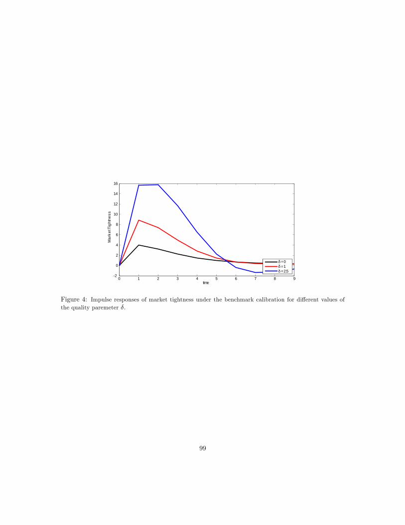
0 1 2 3 4 5 6 7 8 9­2

0

2

4

6

8

10

12

14

16

time

Mar

ket T

ight

ness

δ = 0δ = 1δ = 2.5

Figure 4: Impulse responses of market tightness under the benchmark calibration for di¤erent values ofthe quality paremeter �.

99

The Search and Matching Model when Agents are Learning

20 May 2011

Abstract

This study investigates the macroeconomic implications from introducing perpetual learn-

ing in a simple search and matching model. When the agents with rational expectations are

replaced with agents that are boundedly rational, the volatilities of vacancies, unemployment

and market tightness are increased signi�cantly. Job creation is connected to the present dis-

counted value of future cash �ows, which means that if agents do not form rational expectations,

their forecasts of future cash �ows are subject to periods of either excess optimism or excess

pessimism. Those extra distortions of the agents�forecasts amplify the volatility of job creation.

Therefore, the ampli�cation puzzle arising from the search and matching model might be due

to the strong assumption that agents are rational; thus, when agents need to form multiperiod

forecasts using past data as in Preston (2005) and Eusepi and Preston (2010), the search and

matching model�s ampli�cation potential is enhanced. The model can replicate moments from

quarterly US data from 1955Q1 to 2007Q4. However the more ampli�cation added to the

model through higher gain parameter, the further the correlations generated by the model are

from the ones obtained from US data. That is because higher ampli�cation induces vacancies

to �uctuate around the rational expectations equilibrium less smoothly. Moreover, higher am-

pli�cation through learning worsens the prediction of the model for the slope of the Beveridge

curve.

100

1 Introduction

The search and matching model introduced by Mortensen and Pissarides (1994) has been criticized

by various authors such as Shimer (2005), Fujita (2004) and others for it�s ability to match various

statistics from the US data even though as a �rst pass it seems to outperform the standard RBC

model (Merz (1995), Adolfatto (1996)). Speci�cally, the standard search and matching model

cannot explain the ampli�cation in vacancies, unemployment and market tightness that is observed

in the US data, a drawback that is referred to as the ampli�cation puzzle. Moreover, the model

fails to provide enough propagation either, as the e¤ects of the shock disappear immediately after

the shock dies out. A survey about the problems and possible �xes and critics on the search and

matching model can be found in Cardullo (2008).

Various attempts to enhance the performance of the standard model have been reported. The

�rst wave of attempts involved changes in the wage formation such as including wage rigidity. Those

attempts are criticized by Pissarides (2007) and Haefke, Sonntag and van Rens (2008) implying

wages for new �rms to be too sticky, an assumption rejected by empirical evidence. Another wave

of attempts aimed at changing the calibration in the standard model as in Hagedorn and Manovskii

(2007). However, the higher ampli�cation comes at the cost of making the model too sensitive

to certain policy variables like unemployment bene�ts. The most promising attempts seem to be

those that aim at changing the model�s speci�cation. Although there are numerous attempts to

change the model speci�cation to address the issues I already discussed, in my knowledge there is no

attempt to deviate from the rational expectations assumption, a channel that might be important

in the alignment of the model�s predictions with the data.

The amount of vacancies to be posted every period in a standard search and matching model are

determined by the cost of posting a vacancy and the present value of all future cash �ows the job

is expected to create in the future. The assumption that agents have rational expectations is very

crucial in the determination of vacancies and jobs. If agents�forecasts are fully speci�ed, vacancies

are barely volatile. However, once deviating from the rational expectations assumption and assume

bounded rationality, agents need to provide forecasts of variables outside their control such as future

101

dividends, �rm revenues and labor supply as well as vacancy costs. Possible misspeci�cations in

the formation of those beliefs are going to have a big impact on vacancy and job creation.

To formulate the above concept in the search and matching framework, I assume the agents have

a fully speci�ed belief system but do not have complete knowledge about equilibrium determination;

that is they do not know how shocks and state variables get mapped into prices and policy variables.

Thus, the agents understand that the solution to their optimization problem implies every variable is

a linear function of the state variables and shocks. What agents do not know exante is the coe¢ cients

that de�ne this linear relation between every variable and the state variables, something known if

agents are fully rational. This deviation from rational expectations through learning is discussed

extensively in the adaptive learning literature in Evans and Honkapohja (2001). I assume agents

form their beliefs for the future through a constant gain learning algorithm. However, I postulate

that agents do not make forecasts of future variables only a period in advance which is the common

assumption in the learning literature. Agents in this model need to make multi-period forecasts as

de�ned in Preston (2005) and Eusepi and Preston (2010). Their �nding is that this deviation from

the literature can enhance the volatility of the standard learning model compared to the common

speci�cation in Evans and Honkapohja. Since the ampli�cation problem in the search and matching

framework is a severe one, I choose to assume agents need to form multi-period forecasts as a way

to confront the issue.

Therefore, in this study agents know that the solution to their optimization problem implies that

every variable in equilibrium is a linear combination of the model�s state variables and shocks. The

only missing piece for the agents is the determination of the forecasts for all the forward looking

variables in their �rst order conditions. Since the agents realize that those future variables are

linear combinations of the state variables, forecasts can be constructed as long as estimates for

those coe¢ cients of the state variables can be obtained. The coe¢ cients are obtained through a

recursive least squares algorithm with constant gain. The parameters are updated period by period

and they are a function of past data.

The agents are boundedly rational in the sense that they make forecasts of future variables

using a misspeci�ed model assuming that over the forecast horizon forecasts will remain intact

102

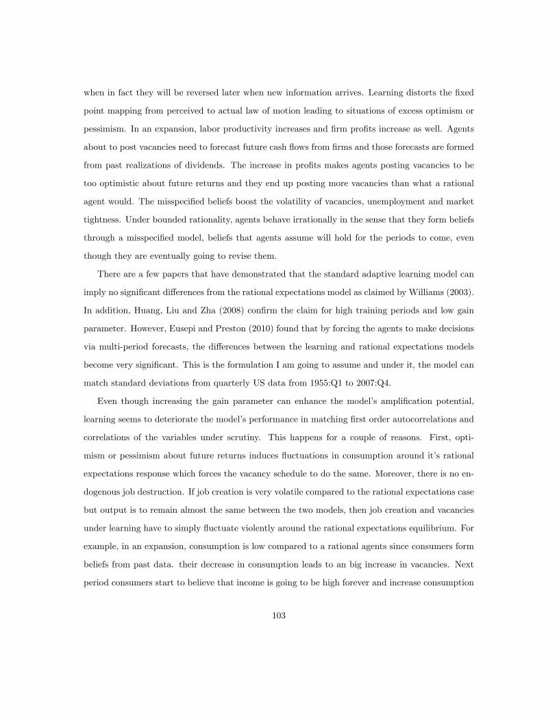
when in fact they will be reversed later when new information arrives. Learning distorts the �xed

point mapping from perceived to actual law of motion leading to situations of excess optimism or

pessimism. In an expansion, labor productivity increases and �rm pro�ts increase as well. Agents

about to post vacancies need to forecast future cash �ows from �rms and those forecasts are formed

from past realizations of dividends. The increase in pro�ts makes agents posting vacancies to be

too optimistic about future returns and they end up posting more vacancies than what a rational

agent would. The misspeci�ed beliefs boost the volatility of vacancies, unemployment and market

tightness. Under bounded rationality, agents behave irrationally in the sense that they form beliefs

through a misspeci�ed model, beliefs that agents assume will hold for the periods to come, even

though they are eventually going to revise them.

There are a few papers that have demonstrated that the standard adaptive learning model can

imply no signi�cant di¤erences from the rational expectations model as claimed by Williams (2003).

In addition, Huang, Liu and Zha (2008) con�rm the claim for high training periods and low gain

parameter. However, Eusepi and Preston (2010) found that by forcing the agents to make decisions

via multi-period forecasts, the di¤erences between the learning and rational expectations models

become very signi�cant. This is the formulation I am going to assume and under it, the model can

match standard deviations from quarterly US data from 1955:Q1 to 2007:Q4.

Even though increasing the gain parameter can enhance the model�s ampli�cation potential,

learning seems to deteriorate the model�s performance in matching �rst order autocorrelations and

correlations of the variables under scrutiny. This happens for a couple of reasons. First, opti-

mism or pessimism about future returns induces �uctuations in consumption around it�s rational

expectations response which forces the vacancy schedule to do the same. Moreover, there is no en-

dogenous job destruction. If job creation is very volatile compared to the rational expectations case

but output is to remain almost the same between the two models, then job creation and vacancies

under learning have to simply �uctuate violently around the rational expectations equilibrium. For

example, in an expansion, consumption is low compared to a rational agents since consumers form

beliefs from past data. their decrease in consumption leads to an big increase in vacancies. Next

period consumers start to believe that income is going to be high forever and increase consumption

103

too much. This makes vacancies too low that period and the story continues going from too high

to too low vacancy creation. This implies that vacancies are going to �uctuate violently around

the rational expectations case, a behavior that forces all variables to be less autocorrelated and the

correlation of vacancies and unemployment (Beveridge curve) less negative or even positive after a

speci�c value for the gain parameter.

The second section presents the model where all the details about the agents and their decisions

as well as the bargaining problem of the �rm and worker are determined. Moreover in the same

section, I present the formation of beliefs which eventually in�uences the actual law of motion of

the model economy. The third section presents the calibration along with the results.

2 The Model

I develop in the next section a simple search and matching model in the spirit of Mortensen and

Pissarides (1994) in discrete time. There is a large number of identical households containing

a continuum of consumers each. This assumption guarantees market completeness as in Merz

(1994) because each household has the same ratio of employed to unemployed people and the same

portfolio each period. Households choose every period their consumption basket and vacancies

to post. Posting vacancies is the means of job creation as in the standard model. A household

that manages to successfully create a �rm/job by posting a vacancy is the rightful owner of the

particular �rm and is entitled to any dividend the �rm can pay for as long as it survives. Firms

are jobs consisting of a single worker each and they appear and vanish according to the standard

search and matching literature.

The main di¤erence is the departure from the rational expectations framework by assuming that

agents are learning and can thus have non rational beliefs when forming expectations. The learning

framework is of the kind presented in Preston (2005) and Eusepi and Preston (2010) where agents

use multi-period forecasts upon making optimal decisions instead of making forecasts only a period

in advance as in the standard learning model of Evans and Honkapohja (2001).

104

2.1 Households

There is a large number of households, each one consisting of a continuum of consumers that can

be either employed or unemployed. The hth household attempts to maximize the following utility

function each period:

U�Cht ; L

ht

�=

�Cht�1��

1� � �Nht

�Lht�1+`

1 + `

The household gets utility from consumption Cht and disutility from the labor e¤ort Lht supplied

by each of the Nht employed workers in the household. The �ow budget constraint in terms of the

real good is:

Cht + Pvt V

ht =

�Ih �Nh

t

�bht +N

ht w

ht L

ht + T

ht + ~Nh

t dht

where P vt is the cost per vacancy posted and Vht the vacancies posted by the particular household.

The households can post vacancies. Whenever a vacancy is �lled with a worker, the household

obtains the shares of the �rm that is created by the successful match. The right hand side of

the budget constraint includes the period t income from various sources. The government pays

unemployment bene�t bht to the Ih �Nht unemployed workers in the household denoting as Ih the

measure of the household. The labor income comes from the Nht employed household members

providing Lht hours each and getting compensated wht units of the real good per unit of e¤ort. The

transfers from the government are indicated by Tht . The household is entitled to dividend payment

dht from each of the ~Nht �rms the household owns. The evolution of the household�s stock portfolio

is

~Nht+1 = (1� �) ~Nh

t + qtVht

where the number of �rms the household owns next period ~Nht+1, equals the surviving �rms from last

period (1� �) ~Nht , since � is the exogenous destruction rate, along with the new �rms created by the

hth household. The new matches are equal to the V ht vacancies posted by the household weighted

by the probability of a vacancy to match qt. The number of employed workers the household has

evolves according to

Nht+1 = (1� �)Nh

t + �t�Ih �Nh

t

�

105

where �t is the probability of an unemployed worker to leave the unemployment pool. The household

has no means of in�uencing the number of employed workers it has since it cannot bene�t it�s own

workers as no control variables appear in the household employment constraint above.

2.1.1 The Household Problem

The state variable for the household is the number of it�s employed workers Nht and the number

of �rms/jobs it owns ~Nht . Even though those two numbers are the same in equilibrium, at the

stage of the optimization problem the household knows that posting vacancies cannot boost the

employment level within its borders. That is because the household realizes that it is too small

compared to the whole economy and therefore the probability one of it�s own workers matches with

a vacancy the household opens is negligible. Moreover, households neglect the fact that all other

households are the same and thus cannot anticipate the identical and coordinated response of every

other household to the same shocks. Thus the state of the economy is t =n~Nht ; N

ht

o. De�ne

with Eht the household�s expectation operator which may be di¤erent from rational. The household

problem then is characterized by the following Bellman equation, since agents are maximized present

discounted utility with discount factor �. That is:

WH (t) = maxfCh

t ;Vht g

nU�Cht��Nh

t G�Lht�+ �EhtW

H (t+1)o

(1)

subject to the budget constraint,

Cht + Pvt V

ht =

�Ih �Nh

t

�bht +N

ht w

ht L

ht + T

ht + ~Nh

t dhht (2)

the law of motion for jobs owned by the household,

~Nht+1 = (1� �) ~Nh

t + qtVht (3)

106

and the law of motion for the household employment level

Nht+1 = (1� �)Nh

t + �t�1�Nh

t

�(4)

The �rst order condition with respect to consumption is:

Uc�Cht�= �ht (5)

where �ht is the Lagrangian multiplier.

The �rst order condition with respect to vacancies is

�EhtWH~Nht+1(t+1) = �

ht

P vtqt

(6)

The envelope condition with respect to ~Nht is

WH~Nht(t) = � (1� �) EhtWH

~Nht+1(t+1) + �

ht dht (7)

Lead (7) one period forward and plug into (6). Then substitute (6) in after leading (6) a period in

advance to get the job creation condition

P vtqt= Eht Q

ht;t+1d

ht+1 + (1� �) Eht Qht;t+1

P vt+1qt+1

(8)

where

Qht;t+1 = ��ht+1�ht

= �Uc�Cht+1

�Uc�Cht� (9)

is the household�s stochastic discount factor. This expression is the job creation condition. The left

hand side of the job creation condition is the cost of a vacancy because P vt is the per unit of time

cost of a vacancy and 1qtis the vacancy duration which is the inverse of the probability a vacancy

�nds a match qt.

107

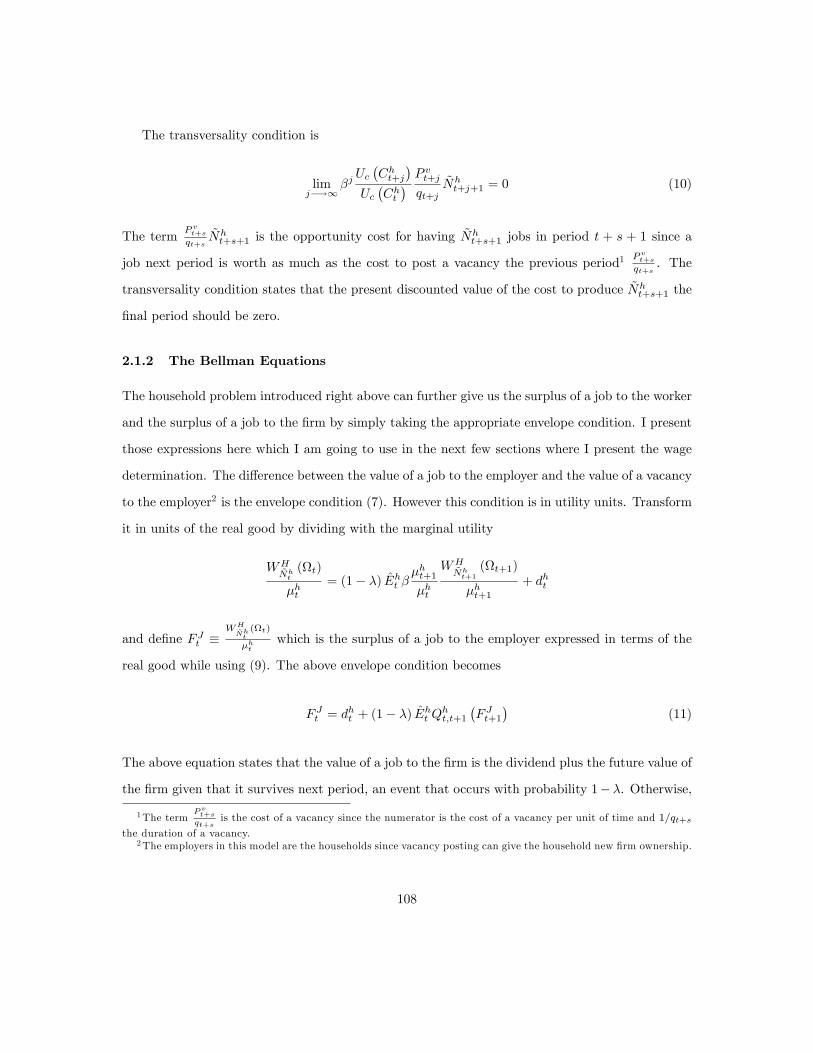
The transversality condition is

limj�!1

�jUc�Cht+j

�Uc�Cht� P vt+jqt+j

~Nht+j+1 = 0 (10)

The termPvt+s

qt+s~Nht+s+1 is the opportunity cost for having ~Nh

t+s+1 jobs in period t + s + 1 since a

job next period is worth as much as the cost to post a vacancy the previous period1Pvt+s

qt+s. The

transversality condition states that the present discounted value of the cost to produce ~Nht+s+1 the

�nal period should be zero.

2.1.2 The Bellman Equations

The household problem introduced right above can further give us the surplus of a job to the worker

and the surplus of a job to the �rm by simply taking the appropriate envelope condition. I present

those expressions here which I am going to use in the next few sections where I present the wage

determination. The di¤erence between the value of a job to the employer and the value of a vacancy

to the employer2 is the envelope condition (7). However this condition is in utility units. Transform

it in units of the real good by dividing with the marginal utility

WH~Nht

(t)

�ht= (1� �) Eht �

�ht+1�ht

WH~Nht+1

(t+1)

�ht+1+ dht

and de�ne F Jt �WH

~Nht(t)

�htwhich is the surplus of a job to the employer expressed in terms of the

real good while using (9). The above envelope condition becomes

F Jt = dht + (1� �) Eht Qht;t+1

�F Jt+1

�(11)

The above equation states that the value of a job to the �rm is the dividend plus the future value of

the �rm given that it survives next period, an event that occurs with probability 1��. Otherwise,

1The termPvt+sqt+s

is the cost of a vacancy since the numerator is the cost of a vacancy per unit of time and 1=qt+sthe duration of a vacancy.

2The employers in this model are the households since vacancy posting can give the household new �rm ownership.

108

if the above is solved forward, then the value of the �rm is the present discounted value of all future

cash �ows for as long as the �rm is expected to survive, which is exactly where our intuition guides

us.

The surplus of a job to the worker, which is the di¤erence between the value of a job and

the value of unemployment to the worker can be found in a similar fashion by taking an envelope

condition in the household problem with respect to Nht , which represents the marginal utility gain

for the household when an extra member switches from unemployment to employment. That is

WHNht(t) = �

ht w

ht L

ht �G

�Lht�� �ht bht + (1� �� �t) EtWH

Nht+1(t+1)

Again I divide the expression above by the marginal utility to represent the above in real units and

de�ne WEt �WU

t �WH

Nht(t)

�htwhich is the value of employment minus the value of unemployment

for the household. That means the surplus of a job to the worker in real units is

WEt �WU

t = wht Lht �

G�Lht�

�ht� bht + (1� �� �t) EtQht;t+1

�WEt+1 �WU

t+1

�(12)

The surplus of a job to the household WEt �WU

t , according to the above equation, is the total

wage wht Lht the employed worker earns minus the disutility of work

G(Lht )�ht

and the unemployment

bene�t lost from the transition to the unemployment pool bht , plus the surplus the household is

expecting to keep enjoying if the job continuous to the next period Et�WEt+1 �WU

t+1

�, an event

with associated probability �t, the probability a worker �nds a job. Equations (11) and (12) de�ne

the pieces of the total surplus from a match, useful ingredients for the determination of the wage

which I present in one of the sections to follow.

2.2 Firms

A job is a �rm which employs a single worker. Therefore, there are Nt employed individuals in the

economy and therefore Nt �rms. Each �rm uses Ljt units of the worker�s e¤ort as input to produce

109

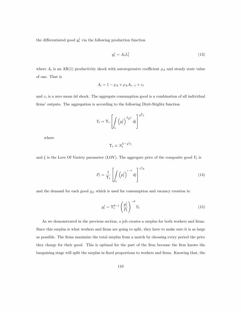
the di¤erentiated good yjt via the following production function

yjt = AtLjt (13)

where At is an AR(1) productivity shock with autoregressive coe¢ cient �A and steady state value

of one. That is

At = 1� �A + �AAt�1 + "t

and "t is a zero mean iid shock. The aggregate consumption good is a combination of all individual

�rms�outputs. The aggregation is according to the following Dixit-Stiglitz function

Yt = �t

24ZNt

�yjt

� ��1�

dj

35 ���1

where

�t � N�� 1

��1t

and � is the Love Of Variety parameter (LOV). The aggregate price of the composite good Yt is

Pt =1

�t

24ZNt

�pjt

�1��dj

35 11��

(14)

and the demand for each good yjt which is used for consumption and vacancy creation is:

yjt = ���1t

pjtPt

!��Yt (15)

As we demonstrated in the previous section, a job creates a surplus for both workers and �rms.

Since this surplus is what workers and �rms are going to split, they have to make sure it is as large

as possible. The �rms maximize the total surplus from a match by choosing every period the price

they charge for their good. This is optimal for the part of the �rm because the �rm knows the

bargaining stage will split the surplus in �xed proportions to workers and �rms. Knowing that, the

110

�rm can do nothing better than maximize that surplus. Even if the �rm is getting a very small part

of the surplus, the best strategy is to maximize it picking the appropriate price. The total surplus

to be maximized is

St = FJt +W

Et �WU

t (16)

Use equations (11) and (12) to substitute the �rm�s and worker�s surpluses in the above expression,

to relate the total surplus to the choice variable of the �rm, its price pjt. In addition, use the fact

that the dividend is djt =pjtPtyjt �w

jtL

jt . After the pre-mentioned substitutions, maximizing the total

surplus is equivalent to maximizing the following:

maxpt

(pjtPtyjt

�pjt

��jtL

jt

�pjt

�)

subject to the demand function, equation (15) and the production function (13). The variable

jt =GL(Ljt)�jt

is the marginal disutility from providing Lt labor units in terms of the real good.

The �rm maximizes the surplus by treating t as �xed. For further details on this result check

Appendix A.

The �rst order condition implies the usual monopoly result that the price is a markup over the

real marginal cost. Ignore the j subscript since all �rms are identical. The relative price of a single

�rm then should beptPt=

�

� � 1GL (Lt)

At

Given that the disutility of an extra unit of labor is GL (Lt) = L`t and the relative price isptPt= N �

t

from equation (14), the �rst order condition of the �rm becomes

N �t =

�

� � 1$L`t�t

1

At(17)

Use the production function (13) and the demand function (15) to transform the above to

N`(1+�)+�t A1+`t =

�

� � 1Y `t�t

(18)

111

which determines output as a function of marginal utility and the state variables and summarizes

the pricing decisions of the �rms.

2.2.1 Nash Bargaining

The �rm and the worker bargain together to set the wage. The current match creates a surplus,

(16), that needs to be split to the two parties. A Nash bargaining regime suggests that the surplus

is split by transferring � part of the surplus to workers and 1�� to �rms. In other words, the above

problem is the same as maximizing the following objective function with respect to the wage

maxwht

n�F Jt�1�� �

WEt �WU

t

��o(19)

The �rst order condition implies

(1� �)�WEt �WU

t

�= �F Jt

where the individual surpluses are envelope conditions from the household problem, equations (11)

and (12). After substituting those expressions in the �rst order condition above, I get the wage

equation

wht Lht = (1� �)

1

1 + `

�Lht�1+`�ht

+ bht

!+ �P vt #t + �p

hrt y

ht (20)

The derivation of the wage is in the Appendix B. The wage at every period is positively related to

the disutility of devoting Lht hours of labor. Higher disutility of labor requires higher wage since the

extra e¤ort needs to be compensated. Higher unemployment bene�t bht grants bargaining power

to workers who can negotiate a higher wage. Either an increase in the cost of a vacancy P vt or

and increase in market tightness #t gives bargaining power to the worker who can eventually leave

the bargaining table with a higher wage. Higher market tightness means workers can �nd a match

more easily relative to vacancies thus workers demand a higher wage in such a scenario.

112

2.3 Household Problem Revisited

The rational expectations assumption is a very convenient tool since it imposes a lot of structure on

the solution of any model. In my model agents separate control variables from forecasting variables

and they provide forecasts for those same variables a rational agent does. Therefore, I force the

agents to form expectations of variables that �rst of all are outside of their control3 . In order to �nd

the appropriate forms of expectations the agents are facing I use the �rst order conditions of the

agents without imposing any equilibrium conditions on them. For example the household doesn�t

know that all other households are the same or that the other workers are receiving the same wages

or what the pricing formula of a �rm is. In the formation of expectations agents know only about

themselves. Any future variables that are outside the agents�control need to be forecasted using

the state variables as regressors.

The solution to the household problem involves the combination of the job creation condition

(consumption and vacancies FOCs combined) which I repeat below

P vtqt= (1� �) Eht Qht;t+1

P vt+1qt+1

+ Eht Qht;t+1d

ht+1 (21)

and the household budget constraint which I also repeat

Cht + Pvt V

ht = N

ht WtL

ht +

�Ih �Nh

t

�bht + ~Nh

t dht + T

ht

As I already mentioned in the household section, the variable Nht is the number of employed people

within the household while ~Nht the number of �rms/jobs the household owns. In equilibrium ~Nh

t

and Nht are the same and equal to the economy-wide employment but households do not know that

simply because they ignore that every other household is identical to their own in every aspect.

The equation for the law of motion of ~Nht is

~Nht+1 = (1� �) ~Nh

t + qtVht (22)

3 If on the contrary a variable to be forecasted is in the agent�s control, using least squares techniques would meanthat the agent is not behaving optimally.

113

where qt is the probability a vacancy to match. The number of employed workers Nht the household

has, evolves according to

Nht+1 = (1� �)Nh

t + �t�1�Nh

t

�(23)

where �t is the probability an unemployed worker to �nd a job.

Since the government keeps a balanced budget and all households are identical, the transfers to

each household are going to be equal to the unemployment bene�t per household. The households

at this stage cannot possibly have this information. It doesn�t understand that all other households

are identical in every aspect. However, I assume agents know bht and transfers Tht are the same for all

households and also equal in magnitude every period for simplicity. If I did not assume households

possess this knowledge about �scal arrangements, the households would need to provide forecasts

for future unemployment bene�ts and transfers from the government. The budget constraint after

imposing�Ih �Nh

t

�bht = T

ht becomes

Cht + Pvt V

ht = N

ht w

ht L

ht + ~Nh

t dht (24)

2.3.1 The Intertemporal Budget Constraint

The households derive an optimal decision rule for consumption that is valid for arbitrary expec-

tations which requires to combine the Euler equation and the intertemporal budget constraint. It

is a version of permanent income theory in general equilibrium adjusted to a search and matching

framework. For the intertemporal budget constraint �rst substitute in the �ow budget constraint

(24) the law of motion for the number of �rms the household owns, equation (22) to get

Cht +P vtqt

h~Nht+1 � (1� �) ~Nh

t

i= Nh

t wht L

ht + ~Nh

t dht

and rearrange to get a recursive budget constraint

Cht +Kt~Nht+1 = N

ht w

ht L

ht +

�dht + (1� �)Kt

�~Nht (25)

114

where I de�ned Kt =Pvt

qtas the cost of vacancies per unit of time. The per unit cost P vt will be

held constant. Log linearize the budget constraint equation (25) to get

�CCht + ��K �NKt + �K �Nnht+1 =

�N �W �L�Nht + w

ht + L

ht

�+ �d �Ndht +

��d �N + (1� �) �K �N

�nht

The intertemporal budget constraint should relate consumption which is a choice variable for the

household, to forecasts of variables outside of the household�s choice that can be either prices

determined by the market or aggregate variables. The wage is determined by the bargaining problem

between the household and the �rms, hence it is not outside the household�s control. Log-linearize

the wage equation (20). The log-linearized wage equation is

wht + Lht = (1� �)

��N�(1+�) �Y

�1+` �C�W �L

Lht +1� �1 + `

��N�(1+�) �Y

�1+` �C�W �L

Ct

+ ��P v �#�W �L

#t + ��Y

�N �W �L

�phrt + yht

�which apart from consumption it is comprised of variables outside the household�s control. The

wage involves variables such as the demand of the �rm yht , the price the �rm sets phrt and technology

At which are variables the household has no control over them. Appendix C goes over the details

to get to the intertemporal budget constraint

�cEht

1Xj=0

�jvCht+j + �kE

ht

1Xj=0

�jvKt+j = �wEht

1Xj=0

�jvNht+j + �LE

ht

1Xj=0

�jvLht+j (26)

+ �yEht

1Xj=0

�jv rht+j + �dE

ht

1Xj=0

�jvdht+j + n

ht

where rht = phrt + yht denotes �rms revenue and the epsilon variables de�ned in Appendix C

contain structural parameters and steady state values.

115

2.3.2 The Consumption Equation

The intertemporal budget constraint (26) is consisted of expectations of future variables outside of

the household�s control except for the �rst term which is the weighted sum of all future consumption

levels of the household. I need to substitute away future consumption and the way to go is to use

the job creation condition. The asset pricing equation for the jobs which is nothing more than a

rearrangement of the job creation condition (21), is

1 = �EhtChtCht+1

�(1� �)Kt+1 + d

ht+1

Kt

�(27)

after assuming log utility for preferences. Appendix D presents the derivation of the consump-

tion equation which basically combines the log-linearized asset pricing equation for jobs, equation

(27) and the intertemporal budget constraint (26) to eliminate future consumption. The resulting

equation for consumption is:

Cht = (28)

+ �v

��v � � (1� �)� �k

1� �v�c

+1� �v�c

�w��v

1� �v (1� �� ��)1� ��

�Eht

1Xj=0

�jvKvt+j+1

� �v�(1� � (1� �))� 1� �v

�c�d

�Eht

1Xj=0

�jvdht+j+1

+1� �v�c

�v�LEht

1Xj=0

�jvLht+j+1 +

1� �v�c

�v�yEht

1Xj=0

�jvRht+j+1

+1� �v�c

��c

�v1� �v

� �k + �w��v

1� �v (1� �� ��)1� ��

�Kvt

+1� �v�c

��dd

ht + �yR

ht + �LL

ht + n

ht + �w

1

1� �v (1� �� ��)Nht

�

2.4 Equilibrium and aggregate dynamics

All households are identical, having the same ratio of unemployed to employed workers and facing

the same constraints4 . Firms are also identical facing the same technology and decision problems

4However, the foreward looking variables that need to be forecasted arised from the fact that agents do notunderstand that others behave identically.

116

and bargain wages using the same Nash Bargain framework. Since all households are the same, the

h subscripts are dropped and after aggregating all consumption equations (28) for all households

in the economy and de�ne the average expectations as Et =ZEht dh the aggregate consumption

becomes

Ct = �1Et

1Xj=0

�jvKvt+j+1 + �2Et

1Xj=0

�jvdt+j+1 + �3Eht

1Xj=0

�jvLt+j+1 + �4Et

1Xj=0

�jvRt+j+1 (29)

+ �5Lht + �6R

ht + �7d

ht + �8nt + �9K

vt

where �1 = �vh�v � � (1� �)� �k 1��v�c

+ 1��v�c�w�

�v1��v(1�����)

1���

i,

�2 = �v

h1��v�c�d � (1� � (1� �))

i, �3 = 1��v

�c�v�L, �4 = 1��v

�c�v�y,

�5 =1��v�c�L, �6 = 1��v

�c�y, �7 = 1��v

�c�d,

�8 =1��v�c

h1 + �w

11��v(1�����)

i, �9 = 1��v

�c

h�c

�v1��v � �k + �w�

�v1��v(1�����)

1���

iThe above consumption equation is the only equation that involves forward looking variables

that need to be forecasted by agents. The only thing remaining is to present the framework

according to which agents form expectations which is the subject of the following section.

Furthermore, in equilibrium Nt = Nht = ~Nh

t since all households are the same. Therefore the

equilibrium employment law of motion becomes

Nt+1 = (1� �)Nt +Mt (30)

where

Mt = mV1��t U�t

is a constant returns to scale matching function. The above law of motion states that employment

next period is known a period in advance.

After imposing equilibrium conditions on the wage equation (20) and the fact that every worker

117

and �rm are the same, the wage becomes

wtLt = (1� �)

1

1 + `

L1+`t

�t+ bt

!+ �P vt #t + �

YtNt

(31)

Manipulate equation (17) to �ndL1+`t

�t=� � 1�

YtNt

Substitute this into (31) and get

wtLt = (1� �)�

1

1 + `

� � 1�

YtNt+ bt

�+ �P vt #t + �

YtNt

In a similar manner the dividends of the �rms in equilibrium can be expressed as

dt =ptPtyt � wtLt

= (1� �) 1 + `�

� (1 + `)

YtNt� (1� �) bt � �P vt #t

2.5 Expectations

According to (29) the households need to form multi-period forecasts of dividend, vacancy cost,

labor demand and the revenue of the �rm. The households keep in mind that every variable at any

point in time is a function of the state variables and they use econometric techniques to re�ect this

knowledge. The regression equations to be estimated are

dt = �d0 + �

d1nt + �

d2At�1 + "

dt (32)

Kt = �k0 + �

k1 nt + �

k2At�1 + "

kt (33)

Lt = �L0 + �

L1 nt + �

L2 At�1 + "

Lt (34)

rt = �r0 + �

r1nt + �

r2At�1 + "

rt (35)

118

Moreover, as agents need to make multi-period forecasts, they also need to forecast the evolution

of the state variables. In a similar manner employment relates to the past state variables according

to

nt+1 = �n0 + �

n1nt + �

n2 At�1 + "

nt (36)

and the technology shock according to

At = �AAt�1 + "t (37)

I assume the law of motion of the technology shock is exogenous and completely known to the

agents for simplicity5 meaning that no estimate for �A is necessary.

2.5.1 Timing

At the beginning of every period t, agents are equipped with estimates of the coe¢ cients that de-

termine beliefs using data from the previous period t�1. For example, in equation for consumption

(29) the agents need among other things to form expectations for future dividends dt+j . Thus, the

j period ahead forecast of the real dividend is

Etdt+j = �d0;t�1 + �

d1;t�1Etnt+j + �

d2;t�1EtAt+j�1

where �d0;t�1, �d1;t�1 and �

d2;t�1 are belief parameters inherited from the previous period. Agents

tend to assume that the belief parameters above are going to remain �xed for the periods to come

even though they will eventually alter each one of those in subsequent periods. The way to estimate

Etnt+j , is to iterate on equation (36) and EtAt+T�1 by iterating on (37). Therefore, the agents

need estimates not only for �d0, �d1 and �

d2 but also for �

n0 , �

n1 and �

n2 .

5 If alternatively I forced the agents to estimate the law of motion of the technology shock the regression coe¢ cientswould converge very fast to the true values especially because the technology process is exogenous and its realizationis not in�uenced from past forecastng mistakes.

119

2.5.2 Perpetual Learning

The next challenge for the agents is to estimate all those parameters � that correspond to the

regression coe¢ cients in the system above, equations (32) - (35). To achieve this goal the agents

use perpetual learning. De�ne

� �

266664�d0 �k0 �L0 �r0 �n0

�d1 �k1 �L1 �r1 �n1

�d2 �k2 �L2 �r2 �n2

377775 =266664�0

�1

�2

377775as the matrix of regression coe¢ cients. The agents need to estimate the matrix of coe¢ cients �

every period by using as regressors a constant, current and past employment realizations as well as

technology realizations6 . To specify the updating of the estimated parameters I de�ne the following

vectors, the vector of the regressors

qt�1 =

2666641

nt

At�1

377775and the vector of the dependent variables

z0t =

�dt Kt Lt rrt nt+1

�

The algorithm that recursively de�nes the estimated parameters is:

�t = �t�1 + gR�1t qt�1

�zt � �0t�1qt�1

�0(38)

Rt = Rt�1 + g�qt�1q

0t�1 �Rt�1

�(39)

6 I include a constant in the estimation process even though the model has a steady state of zero since agentsbeing irrational they might believe the steady state might be changing.

120

where g 2 (0; 1) is a constant gain parameter7 . Agents estimate �t at the end of the period t after

making consumption and vacancy decisions. This means that the period t decisions are based on

the estimated parameters �t�1.

The derivation of the actual law of motion (ALM) for consumption is presented in Appendix E.

The ALM for consumption is

Ct = 0 +1nt+1 +2At + �5Lht + �6r

ht + �7d

ht + �8nt + �9K

vt

where 0 = 11��v

��1�

k0;t�1 + �2�

d0;t�1 + �3�

L0;t�1 + �4�

R0;t�1

�+ �v1��v

�n0;t�11��v�n1;t�1

��1�

k1;t�1 + �2�

d1;t�1 + �3�

L1;t�1 + �4�

R1;t�1

�,

1 =1

1��v�n1;t�1

��1�

k1;t�1 + �2�

d1;t�1 + �3�

L1;t�1 + �4�

R1;t�1

�and

2 =

264 �v1��v�A

11��v�n1;t�1

�n2;t�1��1�

k1;t�1 + �2�

d1;t�1 + �3�

L1;t�1 + �4�

R1;t�1

�+ 11��v�A

��1�

k2;t�1 + �2�

d2;t�1 + �3�

L2;t�1 + �4�

R2;t�1

�375

2.6 The solution

The following log-linear equations de�ne the solution of the model along with the recursive rule for

updating beliefs, equations (38) and (39).

The ALM for consumption

Ct = 0 +1nt+1 +2At + �5Lht + �6r

ht + �7d

ht + �8nt + �9K

vt

The relative price

Lt = Yt � (1 + �) nt � At

The demand

rht = Yt � nt7Higher g means the households weight current observations more heavily than the past ones. For example a gain

value of 0.005 for example means that observations 30 years ago receive a weight of 0.55 and observations 100 yearsago 0.14.

121

Dividends

�ddt = (1� �)1 + `�

� (1 + `)

�Y�N

�Yt � nt

�� �

�P v �#

�Kt

The foc of the �rm�s problem

[` (1 + �) + �] nt + (1 + `) At = `Yt + Ct

The technology process

At = �AAt�1 + "t

The law of motion for employment

nt+1 =

�1� �� �

� �N

1� �N

��nt + �

1� ��

Kt

The cost of vacancies after assuming P vt is a constant

Kt = Pvt + �#t = �#t

The wage equation from bargaining

�w�L!t = (1� �)1

1 + `

� � 1�

�Y�N

�Yt � nt

�+ �

�P v �#

�Kt + �

�Y�N

�Yt � nt

�

where

!t = wt + Lt

and the resource constraint which after some manipulations becomes

�CCt +�P v �V

�Kt = �Y Yt +

�N

1� �N�P v �V nt

122

Appendix F presents the model to be estimated in a form that can be easily simulated using any

software.

3 Simulation and results

I calibrate the model by setting the parameters to common values used in the search and matching

literature. I simulate the model in an attempt to match statistics from the US data from 1955:Q1

to 2007:Q4, for a total of 212 observations. I run the algorithm 3000 times. Each simulation

corresponds to 7000 + T periods. The �rst 7000 periods are ignored just to guarantee convergence

of the estimated parameters to the model stationary distribution. Thus, the estimated moments

are obtained from the last T periods. I set T = 212, the number of observations in my data set.

The algorithm is initialized according to Carceles-Poveda and Giannitsarou (2007). The following

sections present the calibration and the main results.

3.1 Calibration

Table 1 summarizes the benchmark calibration. The time discount factor � is set to 0:99, a con-

siderably common value compared to most macroeconomic models. The elasticity of substitution �

for the consumption good is set to 11 as in Boivin and Giannoni (2005) a value which corresponds

to 1.1 markup for the �rms. The inverse of labor supply elasticity `, is set to 2. The elasticity of

the matching function with respect to unemployment is set to 0.4 which matches the elasticity of

0.4 estimated by Blanchard and Diamond (1989). According to Petrongolo and Pissarides (2001)

acceptable values should lie within the interval (0.5 - 0.7). The worker�s share of the surplus � is set

to 0.5 since it is the usual value assumed in the literature even though empirical work has no pre-

dictions for this parameter. Moreover I set unemployment bene�t equal to zero since I attempt to

create ampli�cation without changing the benchmark calibration in Shimer (2005) by much. Hage-

dorn and Manovskii (2005) show that setting the unemployment bene�t to a high value, around

0.9 and the worker�s share of surplus � to a small value, around 0.01, enough ampli�cation can be

created in the basic search and matching model. However Costain and Reiter (2007) argue that

123

Par Name/Explanation Value Source

� time discount factor 0:99 common in macro models� elasticity of subs �nal goods 11 corresponds to 1.1 markup� elast. matching function 0:4 as Blanchard and Diamond (1989)� workers bargaining power 0:5 commonly used. No microevidence` inverse of labor supply elast 2 1

` 2 (0,0.5) Card (1994)� love of variety (LOV) 0 no LOV� s.s unemployment probability 0:6 matches un. duration of 1.67� separation rate 0:04 match 0.06 steady state unempl. rateb unemployment bene�t 0 match data with lowest un. bene�t�A technology parameter 0:9 common in RBC modelsq steady state vacancy probability 0:7 den Haan et al (2000)

Table 1: This is a summary of the baseline calibration.

such a calibration makes the model too sensitive to unemployment bene�t variations, reducing the

quality of it�s predictions for policy analysis.

The steady state unemployment probability � is set to 0.6, as in Cole and Rogerson (1999), which

ends up matching the average unemployment duration of 1.67 observed in quarterly US data. The

steady state probability a vacancy to match q is set to 0.7 as in Cooley and Quadrini (1999) and

den Haan, Ramey and Watson (2000). The separation rate � is set to 0.04. Commonly used values

lie in the interval of between 0.08-0.10. That particular value of � used in this paper is necessary

to lock the steady state unemployment rate to 0.06.

The rest that needs to be chosen is the number of periods the model is simulated before starting

to compute moments and the gain parameter g 2 (0; 1). The total number of periods I run the

model is 7212 periods. The gain parameter g is set to 0.0045, 0.005 and 0.006, since higher values

of the gain parameter imply greater deviations from the rational expectations equilibrium. A gain

parameter of zero replicates the rational expectations model. Common in the literature are values

from 0.007-0.05 as in Branch and Evans (2006), Orphanides and Williams (2005) and others.

3.2 Data

The moments I am after to match come from quarterly US data from 1955:Q1 to 2007:Q1 where

all series are HP �ltered and those moments are summarized in table 2. All variables but the

124

vacancies series on that same table come from data series of the St. Louis economic database.

Speci�cally output is the log of quarterly real Gdp, unemployment rate the civilian unemployment

rate, vacancies is the log of Help-Want advertising and the wage the hourly earnings in the business

sector. I simulate the model to match second moments from quarterly US data. Table 2 presents

a few statistics from the US data which are basically the target moments. It is clear from the

table that the ampli�cation task is very challenging. Vacancies are nearly nine times the volatility

of output, unemployment nearly seven times the volatility of output while tightness is as large

as seventeen times more volatile than output. Moreover, the correlation between vacancies and

unemployment around -0.9 implies a high slope for the Beveridge curve. All series are highly

autocorrelated, pointing out that all those variables are very persistent. The standard deviation

of the wage is a bit higher than half the standard deviation of output. The low volatility of the

wage compared to output has been an issue in the RBC literature as pointed out by Christiano and

Eichenbaum (1992). As a matter of fact, in the search and matching literature the wage volatility

implied by the standard model is exaggerated even more.

3.3 Results

Consider the impulse responses to a unit technology shock presented in �gure 1 (or �gure 2). The

blue dashed lines correspond to the perpetual learning model with gain 0.005 (or 0.006 for �gure

2) and each one is the median point-wise response function from 3000 simulations. The red solid

lines corresponds to the impulse responses from the rational expectations model. In the rational

expectations case, a rise in labor productivity increases the demand for labor hours on impact. In

the following periods changes in production are mostly met by changes in employment and that

is why labor hours become negative once employment starts increase the period after the shock.

The increase in the demand for hours increases both hours and the real wage. Since the shock

is persistent and agents fully rational, the increase in productivity creates a wealth e¤ect since

consumers forecast an increase in their future income. This wealth e¤ect increases consumption

on impact. The di¤erence between income and consumption is simply vacancies. What consumers

don�t consume they use it to create jobs. The increased consumption shifts the labor supply curve

125

upwards and along with the shifted labor demand, the wage overshoots and the labor hours are

barely increased.

Learning changes the picture a bit as the blue dashed lines in �gure 1 suggest. The increase

in labor productivity again raises labor demand and increases wages and hours on impact through

a substitution e¤ect. However, the di¤erence with rational expectations is that agents learn using

past data which dampens the wealth e¤ect. Since consumption is determined from expectations

of future income and agents learn using past data, on impact consumption does nor rise as much

as the rational expectations case. That is why the response of consumption in �gure 1 is lower on

impact from the rational expectations response. The low response of consumption leads to higher

vacancy posting since whatever is not consumed it is invested in new �rms. This explains the large

response of vacancies under learning on impact. The next period expectations about future income

are revised and agents perceive that the big increase in employment is going to persist forever as

well as the large wages enjoyed the previous period and thus the consumers increase consumption

above the rational expectations response. This implies that once output is realized on the second

period, vacancies are going to be too few, because the consumption increase crowds out investment.

In other words, the second period, optimism about future returns increases consumption too much

and diminishes vacancy posting. This story continues until the responses return to their long-run

values leaving the vacancies response �uctuating around the rational expectations response.

Moreover, as Huang, Liu and Zha (2008) �nd, this decrease in consumption on impact (lower

wealth e¤ect) is going to have a di¤erent impact compared to rational expectations case. In their

model, lower consumption means the labor supply is not going to shift upwards as much, leading

to lower wages and higher labor hours. In my model the decrease of the impact of the wealth e¤ect

increase hours compared to the rational expectations case, in line with the �ndings of the authors

above. However, in my model wages are increased in the learning model besides the decrease of

the wealth e¤ect. The reason is because the wage structure is much di¤erent now than in the

standard RBC case. The dampening of the wealth e¤ect decreases the wage on the �rst hand but

on the other hand the rise in vacancies increases market tightness too much which gives bargaining

power to workers that grants them a higher wage contract. Thus in my model, the decrease in

126

consumption leads to a big increase in the wage due to the importance of outside opportunities in

the wage formation in the search and matching framework.

The tables from 3 to 6 present the same set of statistics as table 2 and are obtained from

simulating the model for di¤erent gain parameters. Table 3 corresponds to gain g=0 or the ra-

tional expectations model. Tables 4 to 6 represent the models with perpetual learning and each

table summarizes the statistics gathered by simulating the models with constant gains g=0.0045,

g=0.005 and g=0.0055 respectively. Let us focus on the ampli�cation e¤ects of the models which

are isolated in table 7. Each row presents relative standard deviations of vacancies, unemployment

market tightness and the real wage with respect to output, from data and di¤erent model speci�-

cations. The �rst row of numbers corresponds to the statistics from US data. The second row is

the rational expectations model�s moments. Clearly the rational expectations model cannot gener-

ate any ampli�cation for vacancies unemployment and market tightness. Although in this model

speci�cation the wage volatility is a bit exaggerated, it is not as high as the models with perpetual

learning. From the third row to the end are the statistics obtained from the learning models. As

the gain parameter g increases the model�s ampli�cation increases dramatically. When the constant

gain parameter g is set to 0.0055 the model can amplify the labor market variables as much as the

data suggests.

The extra ampli�cation in the model with perpetual learning arises because agents make fore-

casts using a misspeci�ed model. The agents�beliefs stemming from the misspeci�ed forecasting

model are assumed to last forever while in fact the agents are going to revise them the following

period. This behavior is what creates extra ampli�cation in the model, boosting the volatilities of

vacancies and unemployment signi�cantly.

Although added volatility seems to be bene�cial for most of the labor market variables, I cannot

claim the same thing for the wage series. Wage in the data is a little more than half as volatile as

output. The rational expectations seems to be closer to the data than the rest of the models, even

though it attains a value that is more than double the one observed in the data. Learning does not

seem to resolve this issue but it was absolutely expected. Take a look again at the wage implied by

the search and matching model, equation (31). When vacancies increase and unemployment shrinks,

127

market tightness becomes very large since tightness #t equals vacancies over unemployment Vt=Ut.

This means that boosting the volatilities of vacancies and unemployment immediately increases the

volatility of the real wage. This is due to the fact that outside opportunities tend to a¤ect the wage

in the search and matching literature due to Nash bargain. More vacancies than unemployed gives

bargaining power to workers because they can break the match at any time and �nd a job elsewhere

very easily, while for the �rm to �nd another match is relatively more di¢ cult. Since tightness is

very volatile, the wage becomes too volatile and absorbs most of the e¤ect of the shock. However,

the increased volatility that appears in the learning model does not come from a change in the wage

formation. It comes from mistakes in the formation of forecasts about the future dividends of the

�rms. Therefore, the wage is going to be more volatile than in the rational expectation model�s case,

since there�s nothing to keep tightness from causing the wage to overshoot. Increasing the volatility

of the forecasts of future dividends boosts the volatility of vacancies and unemployment but also

that of the wage. In a more complex model with sticky wages for continuing �rms, the volatility

of the wage could be signi�cantly reduced to the data levels. Moreover, such a modi�cation would

not sacri�ce the ampli�cation for the rest of the variables. On the contrary, it would even provide

some additional ampli�cation on top.

Once persistence is examined the picture changes a lot. The responses in �gure 1 suggest that

the responses from perpetual learning die out more slowly. However, observing the autocorrelations

of the variables in tables 3 to 6 which are summarized in table 8, one can infer that the rational

expectations model can outperform the learning model. When the gain parameter increases, the �rst

order autocorrelation of vacancies becomes negative. The reason lies in the behavior of vacancies

which is the main reason for the distortion in autocorrelations. It is easier to visualize what is

going on if you take a look at �gure 3 where I present the mean impulse response of vacancies

under rational expectations after a unit technology shock, along with the mean impulse responses

of vacancies from the learning model for di¤erent gain parameters. The red solid line corresponds to

the rational expectations case while the blue dashed line is the learning model with gain g=0.005,

the black dotted line is the learning model with gain g=0.0055 and the mixed line corresponds to

g=0.006. It is obvious that higher gain leads to higher volatility for vacancies by making vacancies

128

�uctuate around the rational expectations response. When vacancies one period is above average,

next period it appears below average and so on. This makes the degree of autocorrelation in

vacancies to drop as the gain parameter increases and when the gain is su¢ ciently large it even

becomes negative. The impulse response for vacancies in the learning model is high on impact

and the period following the shock and then goes below the response of the rational expectation

model and then on top again. It �uctuates around the rational expectations response. This kind

of movement is what distorts all correlations in the model.

In this model output does not seem to be much a¤ected by expectations. I don�t mean that

income is not a¤ected at all, but the e¤ect of learning on output is rather mild. The behavior of

the output response can be understood by examining the foc of the �rm which I repeat below

`nt + (1 + `) At = `Yt + Ct

Set � = 0 which is the benchmark calibration and use the log-linear resource constraint

�Y Yt = �CCt + �P v �V Vt

to substitute for consumption. That is

� �Y�C+ `

�Yt = `nt + (1 + `) At + �P v

�V�CVt

The parameter �Y�C' 1 because �Y = �C+ �V and �V should be as small as possible not only to be able

to match US data facts, but also to be able to have any ampli�cation in the model8 . The output

response is then equal to

Yt = At +`

1 + `nt + �P v

�V�CVt

The change in output equals the change in technology At plus a fraction of the change in employment

`1+` nt plus a fraction of the change in vacancies. Employment steady state is very high and thus

8Deviations of vacancies from the steady state are larger the smaller the vacancy steady state is. Assuming a highvalue for Vacancy steady state value diminishes the model�s ampli�cation potential.

129

deviations from it are very small. Moreover, the steady state of vacancies is too small which makes

the term �P v�V�Cequal to 0.03. Even if Vt is as large as 3 times the response of output, output is barely

volatile. Learning can boost employment and vacancies but unemployment response cannot be too

high since it�s steady state is high and also the e¤ect of vacancies on output is small since vacancies

are a very small part of aggregate Gdp. Therefore, when expectations determine consumption,

output is barely a¤ected and vacancies are whatever part of the output is not consumed. The

ability of the learning to a¤ect output is crucial in order to replicate the results as in Eusepi and

Preston (2010).

To summarize, it is important to note that the greater ampli�cation seems to come at the

cost of distorting correlations, but this is not solely due to the way beliefs are formed. It is also

a¤ected by the fact that the simple search and matching model I have used, implies output is not

much in�uenced by expectations. By employing a di¤erent framework, the way vacancies �uctuate

can be reduced enhancing the performance of the model against autocorrelations. However it is

important to note that the search and matching model needs a very high ampli�cation boost to

match the data as can be seen by comparing the �rst two rows of table 7. If this ampli�cation is

solely provided by a perpetual learning framework, there is inevitably going to be some trade-o¤

between ampli�cation and correlation. The model with gain g=0.0045 can amplify the vacancies

and unemployment processes by more than 50% compared to the rational expectations model.

However, the correlations remain more or less the same between the two models, denoting that

learning is not distorting the rest of the model implied moments. Nevertheless, the gap between

the volatilities in the data and the model with g=0.0045 is still signi�cant. The ampli�cation that

is needed to eliminate the gap is around nine times the ampli�cation in the rational expectations

model which forces me to employ higher values for the gain parameter creating a trade-o¤ between

success in providing ampli�cation over correlation in the model.

The most important e¤ect of the distortion in the correlations implied by the model with per-

petual learning is the reduction in the correlation between vacancies and unemployment. Table

9 presents the correlations between vacancies and unemployment which de�nes the slope of the

Beveridge curve. The correlation of the two variables in the data is high and negative with a value

130

of -0.91. The rational expectations model implies a correlation of -0.63 and it is not even close to

match the data. The models with higher gain imply an even lower correlation in absolute value

and a positive correlation in the last two model speci�cations. Note that the correlations are low in

absolute value even though vacancies are procyclical and unemployment countercyclical. As �gure

1 demonstrates, while new matches start producing a period after the match, on impact, vacancies

achieve their highest value while unemployment remains at zero. When unemployment increases

later on, vacancies are already fading away inducing a very low correlation between the two vari-

ables. For higher gains, vacancies become negative when unemployment is at it�s pick, inducing

even positive correlation for vacancies and unemployment. As the gain parameter increases this

correlation drops. Keep in mind that the ampli�cation puzzle arises because in the wage equation

(31) the market tightness is too volatile making the wage too depended on outside opportunities.

The increased volatility in the wage decreases the volatility in dividends and leaves vacancies barely

a¤ected. Imagine a situation where vacancies and unemployment are highly positively correlated.

That would imply that market tightness #t would not be too volatile simply because vacancies and

unemployment cancel each other out. Such a model would support high volatilities for vacancies

and unemployment simply because the two variables cancel each other out and wages do not crowd

out vacancies. In the current models, vacancies and unemployment are not as highly negatively

correlated as the data suggest. This makes the ampli�cation issue in the model a bit less severe

simply because market tightness is not as volatile as it should be if vacancies and unemployment

didn�t partly o¤set each other. Therefore the models with high gain parameter provide some am-

pli�cation for the wrong reason. Since tightness is less volatile than it would if the slope of the

Beveridge curve was around -0.9, wage becomes less volatile and it�s not as e¤ective in absorbing

most of the e¤ect of the shock.

3.4 Alternative Model Speci�cation

The model I presented in this paper, besides the alternative expectations assumption, it di¤ers

from the standard search and matching model in two areas. First of all, in my model future cash

�ows are discounted by a stochastic discount factor instead of a constant one. The addition of

131

a stochastic discount factor can boost job creation a little bit. The reason is because agents are

risk averse and job/�rm creation provides some insurance to the investor. After a productivity

shock income increases. Vacancies are posted on the current period where income is high and

they will make payments next period if a match is found, where income is lower. This means that

vacancy posting becomes a form of insurance and agents would keep posting vacancies even if the

dividend they are promised to pay next period is really small. However, when the discount factor

is constant, agents would stop posting vacancies when dividends are expected to be too low. Risk

neutral agents are only concerned about returns and not the state of the business cycle the cash

�ows appear. Nonetheless, the ampli�cation created by the inclusion of a stochastic discount factor

is not signi�cantly high. Nevertheless, assuming that agents are actually risk averse is a realistic

assumption.

Moreover, another di¤erence between my model and the standard case is that I assume there

is also labor e¤ort decision for the �rm, while the standard search and matching model allows

changes in labor only through the extensive margin. I can replicate the results of a model with

just the extensive margin by setting the parameter de�ning disutility for labor ` to zero9 . Table

10 compares the benchmark learning model with a gain of 0.005 for di¤erent parameters for the

disutility of labor `. The model with no intensive margin (` = 0) can match the ampli�cation

in the US data more easily while the one with ` = 2 (the benchmark model parameterization)

cannot. Since the disutility from labor in the model with no extensive margin is constant, the wage

is not as responsive and therefore it creates some extra pro�t margin for the �rms compared to the

benchmark model, which results in an additional wave of vacancy postings. After a productivity

shock, on impact, labor hours/e¤ort increase. Agents expect next period�s hours will be as high and

infer that the disutility of labor (the cost of labor) will be high for the periods to come. Therefore,

agents expect pro�ts to be lower and end up posting less vacancies on impact. This channel is

9Solve the model I presented above and simply change the following assumptions:Assume the aggregator function

is Yt =

"1R0

�yjt

� ��1�dj

# ���1

and production function is yjt = Njt where N

jt is the number of workers the j

th �rm

employes. Assume the disutility for labor in the utility function is Nht G (L) where the function G (L) is now constant.

Solving the model under this speci�cation and solving my original model with ` = 0 is going to produce the samedynamics.

132

absent if the intensive margin is eliminated and the disutility of labor is constant. This observation

can be con�rmed by comparing the last columns of table 10 where it shows that the volatility of

the wage in the models without the extensive margin is much lower than the benchmark model.

Decreasing the volatility of the wage signi�cantly is crucial for the search and matching model.

Despite the fact that the model with ` = 0 seems to outperform the benchmark model, the main

reason I keep the benchmark model as the one with both the intensive and extensive margin is

simply because it is more realistic10 .

3.5 The Distribution of Beliefs

The formation of beliefs is crucial for my result since the substitution or rational beliefs with

boundedly rational beliefs is what creates the additional ampli�cation in this model. The way

beliefs are updated using perpetual learning through equations (38) and (39), suggests that as time

passes, beliefs will not converge to a particular value but to a distribution, since agents tend to

forget old data up to a certain threshold that is controlled by the gain parameter.

Figure 5 presents the densities of the belief coe¢ cients after simulating the model for a gain

of 0.005. The number of observations in each density are around 2,000,000 data points. Each

row corresponds to a variable that is forecasted and each column to the state variable used as a

regression for the formation of those forecasts. It is obvious that there is a very high dispersion for

each belief coe¢ cient. This is what actually creates the extra volatility in the learning model. This

dispersion endogenously creates shifts in agents�expectation that becomes a source of business cycle

�uctuations and probably the source that seems to be ignored in the standard search and matching

literature.

The medians of the densities for di¤erent gain parameters are reported in table 11 along with

the means. Although there is a very high scattering around the median, it seems to be very close

to the rational expectations case even though the mean states that the distributions are skewed.

Figure (4) shows the evolution of beliefs when instead of a constant gain I use a decreasing gain of

the form gt = 1=t. Each row of 3 graphs represent a coe¢ cient for a particular variable that needs

10Mind that in the standard search and matching model there is no intensive margin.

133

to be forecasted by agents. Each row represents the coe¢ cient of the particular state variable. The

blue lines correspond to the beliefs while the red �at line marks the rational expectations coe¢ cient.

All coe¢ cients eventually tend to converge to their rational expectations counterpart.

The impulse responses in �gure (1) are di¤erent than the rational expectations responses on

impact which might suggest that the distribution of believes is not centered at the rational ex-

pectations belief coe¢ cients even though the conditions for E-Stability are satis�ed and the gain

coe¢ cient is between zero and one. The reason is because of the non-linear dynamics the belief

system is following. Under decreasing gain, the coe¢ cients tend to converge to the rational ex-

pectations beliefs solely from the same side. For example, no matter how the belief framework is

initialized, the coe¢ cient of the state variable one for the dividend process, always converges from

above as can be seen in the second graph on the �rst row of �gure (4) . Therefore,as the constant

gain parameter increases, the belief parameters tend to converge to a distribution with means a bit

shifted from the rational expectations parameters.

4 Conclusion

In this study I consider a perpetual learning algorithm in an attempt to enhance the standard

search and matching model�s performance. The ampli�cation problem of the standard search and

matching model is a very severe one and very e¤ective ampli�cation mechanisms are needed for the

puzzle to be successfully resolved. Learning algorithms tend to have mild impact in the dynamics of

macroeconomic models as studies like Williams (2003) have shown. However, by assuming agents

rely on multi-period forecasts as in Eusepi and Preston (2010) rather than forecasts at most a

period in advance , the ampli�cation prospective of the learning model is signi�cantly improved.

The learning model can provide ampli�cation to match moments from the US data from 1955:Q1

to 2007:Q4. However, the extra ampli�cation comes at the cost of distorted correlations since

the more ampli�cation is added the more vacancies �uctuate around the rational expectations

equilibrium achieving a low autocorrelation coe¢ cient that a¤ects the autocorrelation of every single

variable in the model. Moreover, learning distorts the correlation of vacancies and unemployment

134

known as the Beveridge curve implying even a positive slope for the Beveridge curve as the gain

parameter increases.

The model could perform better in a more complex setup where there exists some mechanism

that could potentially keep vacancies in a smoother path. For example, endogenous job destruction

could open another channel for some corrections in employment to take place without violent shifts

in vacancies to be necessary. This is something that I tend to investigate in future research.

References

[1] Boivin, J., and M. P. Giannoni (2005). "Has Monetary Policy Become More E¤ective?", NBER

Working Paper No. 9459

[2] Carceles-Poveda and Giannitsarou (2007). "Asset Pricing with Adaptive Learning", forthcom-

ing, Review of Economic Dynamics.

[3] Cardullo, G., (2008). "Matching Models Under Scrutiny: Understanding the Shimer Puzzle",

Discussion Papers, Department des Sciences Economiques 2008009.

[4] Cole, H., and R. Rogerson (1999). "Can the Mortenses-Pissarides matching model match the

business cycle facts?", International Economic Review 40(4), 933-959.

[5] Cooley, T.F., and V. Quadrini (1999). "A Neoclassical Model of the Philips Curve Relation",

Journal of Monetary Economics 44(2), 165-193.

[6] Costain, J., and M. Reiter (2007). �Business Cycles, Unemployment Insurance, and the Cali-

bration of Matching Models�, Journal of Economic Dynamics and Control, forthcoming.

[7] Davis S., J. Haltiwanger, and S. Schuh (1996). Job Creation and Destruction, The MIT Press.

[8] Den Haan, W., G. Ramey, and J. Watson (2000). "Job destruction and Propagation of Shocks",

American Economic Review, 90(3), 482-498B

[9] Eusepi and Preston (2008). "Expectations Learning and Business Cycle Fluctuations", NBER

Working Papers 14181.

135

[10] Evans and Honkapohja (2001). "Learning and Expectations in Economics", Princeton Univer-

sity Press.

[11] Fujita, S., (2003). "The Beveridge Curve, Job Creation and the Propagation of Shocks", mimeo,

University of California San Diego.

[12] Haefke, C., M. Sonntag, and T. Van Rens (2007). "Wage Rigidity and Job Creation", mimeo,

July.

[13] Hagedorn, M., and I. Manovskii (2005). "The Cyclical Behavior of Equilibrium Unemployment

and Vacancies Revisited", American Economic Review, forthcoming.

[14] Huang, Liu and Zha (2008). "Learning, Adaptive Expectations and Technology shocks", un-

published, Federal Reserve Bank of Atlanta.

[15] Mertz, M., (1995). "Search in the Labor Market and the Real Business Cycle", Journal of

Monetary Economics 36, 269-300.

[16] Mortensen, D., and C. Pissarides (1994). "Job Creation and Job Destruction in the Theory of

Unemployment", Review of Economic Studies 61, 397-415

[17] Orphanides and Williams (2005). "Imperfect Knowledge, In�ation Expectations and Monetary

Policy", The In�ation Targeting Debate, ed. by B. S. Bernanke and M. Woodford. University

of Chicago Press.

[18] Pissarides, C., (2000). Equilibrium Unemployment Theory, The MIT Press.

[19] Pissarides, C., (2007). "The Unemployment Volatility Puzzle: Is Wage Stickiness the Answer?",

mimeo, London School of Economics, November.

[20] Preston, B. (2005). "Learning About Monetary Policy Rules when Long-Horizon Expectations

Matter", International Journal of Central Banking, 1(2), 81-126.

[21] Shimer, R., (2005). "The Cyclical Behavior of Equilibrium Unemployment, Vacancies, and

Wages: Evidence and Theory", American Economic Review 95(1), 25-49.

136

[22] Williams, N. (2003). "Adaptive Learning and Business Cycles", unpublished, Princeton Uni-

versity.

A Appendix

In this section I introduce the surplus maximization for the �rm that is choosing the appropriate

price to set. The �rm is trying to �nd p�t either by maximizing

p�t = argmaxpt

n�F Jt (pt)

�1�� �WEt (pt)�WU

t (pt)��o

or the total surplus

p�t = argmaxpt

�F Jt +W

Et (pt)�WU

t (pt)

The two objectives give the same answer given that the surplus is split according to (1� �)�WEt �WU

t

�=

�F Jt which implies that the surplus is split in �xed portions to �rms and workers.

Therefore, maximizing either of the objective functions leads to

@�F Jt +W

Et (pt)�WU

t (pt)�

@pt= 0

Expand the expression in the brackets using the Bellman equations (11) and (12) in the above �rst

order condition to get:

F Jt +WEt (pt)�WU

t (pt)

= dht + (1� �) Eht Qht;t+1�F Jt+1 (pt+1)

�+ wht L

ht �

G�Lht�

�ht� bht

+ (1� �� �t) EtQht;t+1�WEt+1 (pt+1)�WU

t+1 (pt+1)�

Use the fact that the dividends process is dht = phrt y

ht � wht Lht and the above equation becomes

F Jt +WEt (pt)�WU

t (pt) =ptPtyht �

G�Lht�

�ht+ t:i:p

137

where t:i:p stands for terms independent of price. Therefore, maximizing the surplus becomes

@�F Jt +W

Et (pt)�WU

t (pt)�

@pt=

@

�ptPtyht �

G(Lht )�ht

�@pt

= 0

By the chain rule

@

�phrt�pht�yht�pht�� G(Lht (p

ht ))

�ht

�@pt

=

@

�ptPtyht�pht�� GL(Lht )

�htLht�pht��

@pt

Thus, the objective of the �rm that is trying to maximize the surplus is equivalent to

maxpht

(ptPtyht�pht��GL�Lht�

�htLht�pht�)

by treatingGL(Lht )�ht

as independent of the price pht . This form has interesting implications because

it reveals that in a search and matching model, the cost of labor is the marginal rate of substitution,

the disutility of labor in real units. The standard New Keynesian model assumes that the �rms

solve the exact same problem since the wage in that case equals the marginal rate of substitution,

which is assumed �xed when �rms maximize their pro�t.

B Appendix

This part of the appendix presents the wage determination. The wage in a search and matching

model splits the surplus to workers and �rms in �xed portions. The Nash bargain solution comes

from the following �rst order condition

(1� �)�WEt �WU

t

�= �F Jt (40)

138

which comes from the maximization of the surplus with respect to wage, equation (19). Plug in the

individual surpluses, equations (11) and (12) to get

(1� �) wht L

ht �

G�Lht�

�ht� bht + (1� �� �t) EtQht;t+1

�WEt+1 �WU

t+1

�!= �

�dht + (1� �) Eht Qht;t+1

�F Jt+1

��

plug in the de�nition for the �rm�s dividends

dht = phrt y

ht � wht Lht

and rearrange to get

wht Lht+(1� �)

�G�Lht�

�ht� bht+

!+(1� �� �t) Et (1� �)Qht;t+1

�WEt+1 �WU

t+1

�= �

�phrt y

ht + (1� �) Eht Qht;t+1

�F Jt+1

��

First use (40) in the above expression to substitute WEt+1 �WU

t+1 away. After, use the vacancy

posting condition, equation (6), along with the de�nition F Jt �WH

~Nht(t)

�htand #t =

�tqtto get

wht Lht + (1� �)

�G�Lht�

�ht� bht

!= �phrt y

ht + �P

vt #t

C Appendix

After using the wage equation to substitute away the wage income wt+Lht from the budget constraint

(26) I get

�Ch1� �N 1��

1+`

��N�(1+�) �Y

�1+`i��d �N + (1� �) �K �N

� Ct +� �K � 1

���P v �#�

�d+ (1� �) �K�Kt +

�K��d+ (1� �) �K

� nht+1=

�W �L��d+ (1� �) �K

�Nht +

�C (1� �)��N�(1+�) �Y

�1+`��d+ (1� �) �K

� Lht +� �Y�

�d+ (1� �) �K��N

�phrt + yht

�+

�d��d+ (1� �) �K

� dht + nhtwhere nht are the �rms owned by the h

th household, Nht the number of the household�s employed

workers and Nt the aggregate employment level and evolve according to the laws of motion (which

139

need to be linearized �rst) (22), (23) respectively. The household controls the number of �rms to

own nht by posting vacancies as (22) shows. However, it has no control on the evolution of it�s own

employment level Nht or the aggregate employment Nt because �rst of all it is way too small to

a¤ect aggregate variables and also does not understand that the rest of the households are actually

identical and make decisions in exactly the same way.

De�ne �c =�Ch1� �N 1��

1+` ( �N�(1+�) �Y )

1+` �Ci

[ �d �N+(1��) �K �N], �k =

� �K� 1� �

�Pv �#

[ �d+(1��) �K], �v =

�K

[ �d+(1��) �K], �w =

�W �L

[ �d+(1��) �K],

�L =�C(1��)( �N�(1+�) �Y )

1+`

[ �d+(1��) �K]; �y =

� �Y

[ �d+(1��) �K] �N, �d =

�d

[ �d+(1��) �K]and also de�ne the revenue of the

�rm as rht = phrt + yht

The log linear budget constraint is

�cCt + �kKt + �vnht+1 = �wN

ht + �LL

ht + �y r

ht + �dd

ht + n

ht (41)

Moving it a period in advance

�cCt+1 + �kKt+1 + �vnht+2 � �wNh

t+1 � �LLht+1 � �y rht+1 � �ddht+1 = nht+1

�cCht+1 + �kKt+1 + �vn

ht+2 � �wNh

t+1 � �y yht+1 + �AAt+1 � �pprt+1 � �ddht+1 = nht+1

and substitute it back into (41)

�cCt + �v�cCt+1 + �kKt + �v�kKt+1 + �v�vnht+2

= �wNht + �v�wN

ht+1 + �LL

ht + �v�LL

ht+1 + �y r

ht + �v�y r

ht+1 + �dd

ht + �v�dd

ht+1 + n

ht

Keep doing the same until all nht+j are eliminated for all j = 1; 2; 3; :::

limj�!1

�jvnht+j+1+�c

1Xj=0

�jvCht+j+�k

1Xj=0

�jvKt+j = �w

1Xj=0

�jvNht+j+�L

1Xj=0

�jvLht+j+�y

1Xj=0

�jv rht+j+�d

1Xj=0

�jvdht+j+n

ht

140

The linearized trasversality condition, equation (10) states that both

limj�!1

�jKt+j = 0

and

limj�!1

�j nht+j+1 = 0

Substitute in �v =�K

[ �d+(1��) �K]the fact that in the steady state �K = �

1��(1��)�d. This implies that

�v = �

The limit limj�!1

�jvnht+j+1 = lim

j�!1�j nht+j+1 = 0 from the transversality condition. After taking

expectations the intertemporal budget constraint is the following expression

�cEht

1Xj=0

�jvCht+j + �kE

ht

1Xj=0

�jvKt+j = �wEht

1Xj=0

�jvNht+j + �LE

ht

1Xj=0

�jvLht+j

+ �yEht

1Xj=0

�jv rht+j + �dE

ht

1Xj=0

�jvdht+j + n

ht

D Appendix

Log linearizing the above yields

�KKt = �Eht

h(1� �) �KKt+1 + �ddht+1

i� �

�(1� �) �K + �d

�Eht

�Cht+1 � Cht

�

Keep in mind that at the steady state

�K =�

1� � (1� �)�d

141

which makes the log linearized asset pricing equation

Kt = � (1� �) Eht Kt+1 + (1� � (1� �)) Eht dht+1 � Eht�Cht+1 � Cht

�

The asset pricing equation at period t+ j � 1 is

Eht Kt+j�1 = � (1� �) Eht Kt+j + (1� � (1� �)) Eht dht+j � Eht�Cht+j � Cht+j�1

�(42)

Use the same condition a period back

Eht Cht+j�1 = � (1� �) Eht Kt+j�1 � Eht Kt+j�2 + (1� � (1� �)) Eht dht+j�1 + Eht Cht+j�2

and substitute it in the initial one, equation (42)

Eht Cht+j = � (1� �)

�Eht Kt+j + E

ht Kt+j�1

���Eht Kt+j�1 + E

ht Kt+j�2

�+ (1� � (1� �))

�Eht d

ht+j + E

ht d

ht+j�1

�+ Eht C

ht+j�2

Keep eliminating Cht+j up to the tth period which implies the expected consumption in period t+ j

is

Eht Cht+j = � (1� �) Eht

j�1Xs=0

Kvt+s+1 � Eht

j�1Xs=0

Kvt+s + (1� � (1� �)) Eht

j�1Xs=0

dht+s+1 + Cht (43)

142

Substitute the Euler equation (43) to the intertemporal budget constraint (26)

� (1� �) �c�v

1� �vEht

1Xj=0

�jvKvt+j+1 �

��c

�v1� �v

� �k�Eht

1Xj=0

�jvKvt+j

+ �c (1� � (1� �))�v

1� �vEht

1Xj=0

�jvdht+j+1 +

�c1� �v

Cht

= �wEht

1Xj=0

�jvNht+j + �LE

ht

1Xj=0

�jvLht+j + �yE

ht

1Xj=0

�jv rht+j

+ �dEht

1Xj=0

�jvdht+j + n

ht

where I used the fact that

1Xj=0

�jv

j�1Xs=0

Xt+s+1 =�v

1� �v

1Xj=0

�jvXt+j+1

Isolate in the above expression the terms that need to be forecasted and the ones that are already

known in period t and then solve for consumption

1� �v�c

Cht

= �v

��v � � (1� �)� �k

1� �v�c

�Eht

1Xj=0

�jvKvt+j+1

� �v�(1� � (1� �))� �d

1� �v�c

�Eht

1Xj=0

�jvdht+j+1

+1� �v�c

�wEht

1Xj=0

�jvNht+j +

1� �v�c

�v�LEht

1Xj=0

�jvLht+j+1 +

1� �v�c

�v�yEht

1Xj=0

�jv rht+j+1

+1� �v�c

��v

�c1� �v

� �k�Kvt +

1� �v�c

�ddht +

1� �v�c

�y rht +

1� �v�c

�LLht +

1� �v�c

nht

143

The household knows that the law of motion of the household�s employment level Nht is:

Nht+1 = (1� �� ��) Nh

t + ��t

The same law of motion at period j is:

Nht+j = (1� �� ��) Nh

t+j�1 + ��t+j�1

Solving it backwards up to period t

Nht+j = (1� �� ��)

jNht + �

j�1Xs=0

(1� �� ��)s �t+j�s�1

since the process depend on the exogenous to the household probability for a worker to �nd a job.

The expressionP1

j=0 �jvN

ht+j then becomes

1Xj=0

�jvNht+j =

1Xj=0

�jv (1� �� ��)jNht + �

1Xj=0

�jv

j�1Xs=0

(1� �� ��)s �t+j�s�1

=1

1� �v (1� �� ��)Nht + �

�v1� �v (1� �� ��)

1Xj=0

�jv�t+j

after using the fact that

1Xj=0

�jv

j�1Xs=0

(1� �� ��)s �t+j�s�1 =�v

1� �v (1� �� ��)

1Xj=0

�jv�t+j

144

Plug this fact in the consumption equation above to eliminate Nht+j

Cht

= �v

��v � � (1� �)� �k

1� �v�c

+1� �v�c

�w��v

1� �v (1� �� ��)1� ��

�Eht

1Xj=0

�jvKvt+j+1

� �v�(1� � (1� �))� �d

1� �v�c

�Eht

1Xj=0

�jvdht+j+1

+1� �v�c

�v�LEht

1Xj=0

�jvLht+j+1 +

1� �v�c

�v�yEht

1Xj=0

�jv rht+j+1

+1� �v�c

��c

�v1� �v

� �k + �w��v

1� �v (1� �� ��)1� ��

�Kvt

+1� �v�c

��dd

ht + �y r

ht + �LL

ht + n

ht + �w

1

1� �v (1� �� ��)Nht

�

E Appendix

Now consider the expectation at period t of the law of motion for employment (36) in the t+ j +1

period and iterate back until the expectation becomes a function of variables known at period t

Etnt+j+1 = �n0;t�1

j�1Xs=0

��n1;t�1

�s+��n1;t�1

�jnt+1 + �

n2;t�1

j�1Xs=0

��n1;t�1

�s(�A)

j�1�sAt (44)

Take equations (32) (33), and (34) respectively from period t+j+1 and solve backwards till period

t and substitute in equation (44) and equation (37) each solved backwards from period t+ j+1 till

period t. Therefore the expectations of the dividends, vacancy costs and aggregate output are

Etdt+j+1 = �d0;t�1 + �

d2;t�1 (�A)

jAt

+ �d1;t�1

�n0;t�1

j�1Xs=0

��n1;t�1

�s+��n1;t�1

�jnt+1 + �

n2;t�1

j�1Xs=0

��n1;t�1

�s(�A)

j�1�sAt

!

145

EtKt+j+1 = �k0;t�1 + �

k2;t�1 (�A)

jAt

+ �k1;t�1

�n0;t�1

j�1Xs=0

��n1;t�1

�s+��n1;t�1

�jnt+1 + �

n2;t�1

j�1Xs=0

��n1;t�1

�s(�A)

j�1�sAt

!

EtLt+j+1 = �L0;t�1 + �

L2;t�1 (�A)

jAt

+ �L1;t�1

�n0;t�1

j�1Xs=0

��n1;t�1

�s+��n1;t�1

�jnt+1 + �

n2;t�1

j�1Xs=0

��n1;t�1

�s(�A)

j�1�sAt

!

Etrt+j+1 = �r0;t�1 + �

r2;t�1 (�A)

jAt

+ �r1;t�1

�n0;t�1

j�1Xs=0

��n1;t�1

�s+��n1;t�1

�jnt+1 + �

n2;t�1

j�1Xs=0

��n1;t�1

�s(�A)

j�1�sAt

!

which are all known at period t. Consider the following facts

1Xj=0

�jv

j�1Xs=0

��n1;t�1

�s=

�v1� �v

1Xj=0

�jv��n1;t�1

�j=

�v1� �v

1

1� �v�n1;t�1

1Xj=0

�jv

j�1Xs=0

��n1;t�1

�s(�A)

j�1�s=

�v1� �v�A

1

1� �v�n1;t�1

146

Use the above forecasts and the facts below in the consumption equation (29). The actual law of

motion for consumption becomes

Ct =1

1� �v��1�

k0;t�1 + �2�

d0;t�1 + �3�

L0;t�1 + �4�

r0;t�1

�+

�v1� �v

�n0;t�11� �v�n1;t�1

��1�

k1;t�1 + �2�

d1;t�1 + �3�

L1;t�1 + �4�

r1;t�1

�+

1

1� �v�n1;t�1��1�

k1;t�1 + �2�

d1;t�1 + �3�

L1;t�1 + �4�

r1;t�1

�nt+1264 �v

1��v�A1

1��v�n1;t�1�n2;t�1

��1�

k1;t�1 + �2�

d1;t�1 + �3�

L1;t�1 + �4�

r1;t�1

�+ 11��v�A

��1�

k2;t�1 + �2�

d2;t�1 + �3�

L2;t�1 + �4�

r2;t�1

�375 At

+ �5Lht + �6r

ht + �7d

ht + �8nt + �9K

vt

F Appendix

De�ne

Xt =

26666666666666666666666664

Ct

Yt

dt

!t

Kt

Lt

rt

nt+1

At

37777777777777777777777775The following linear system can be simulated to produce predictions for consumption, output,

dividends, total wage, vacancy cost, �rm demand, �rm price, and employment after a shock to the

147

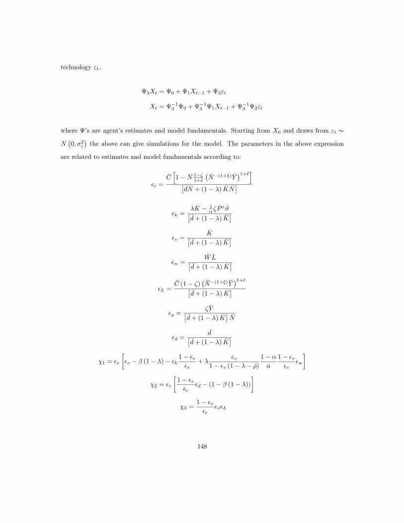
technology "t.

3Xt = 0 +1Xt�1 +2"t

Xt = �13 0 +

�13 1Xt�1 +

�13 2"t

where �s are agent�s estimates and model fundamentals. Starting from X0 and draws from "t s

N�0; �2"

�the above can give simulations for the model. The parameters in the above expression

are related to estimates and model fundamentals according to:

�c =

�Ch1� �N 1��

1+`

��N�(1+�) �Y

�1+`i��d �N + (1� �) �K �N

��k =

� �K � 1���P v �#�

�d+ (1� �) �K�

�v =�K�

�d+ (1� �) �K�

�w =�W �L�

�d+ (1� �) �K�

�L =�C (1� �)

��N�(1+�) �Y

�1+`��d+ (1� �) �K

��y =

� �Y��d+ (1� �) �K

��N

�d =�d�

�d+ (1� �) �K�

�1 = �v

��v � � (1� �)� �k

1� �v�c

+ ��v

1� �v (1� �� ��)1� ��

1� �v�c

�w

�

�2 = �v

�1� �v�c

�d � (1� � (1� �))�

�3 =1� �v�c

�v�L

148

�4 =1� �v�c

�v�y

�5 =1� �v�c

�L

�6 =1� �v�c

�y

�7 =1� �v�c

�d

�8 =1� �v�c

�1 + �w

1

1� �v (1� �� ��)

�

�9 =1� �v�c

��c

�v1� �v

� �k + �w��v

1� �v (1� �� ��)1� ��

�

0 =1

1� �v��1�

k0;t�1 + �2�

d0;t�1 + �3�

L0;t�1 + �4�

r0;t�1

�+

�v1� �v

�n0;t�11� �v�n1;t�1

��1�

k1;t�1 + �2�

d1;t�1 + �3�

L1;t�1 + �4�

r1;t�1

�

1 =1

1� �v�n1;t�1��1�

k1;t�1 + �2�

d1;t�1 + �3�

L1;t�1 + �4�

r1;t�1

�

2 =

0B@ �v1��v�A

11��v�n1;t�1

�n2;t�1��1�

k1;t�1 + �2�

d1;t�1 + �3�

L1;t�1 + �4�

r1;t�1

�+ 11��v�A

��1�

k2;t�1 + �2�

d2;t�1 + �3�

L2;t�1 + �4�

r2;t�1

�1CA

149

3 =

26666666666666666666666664

1 0 ��7 0 ��9 ��5 ��6 �1 �2

1 ` 0 0 0 0 0 0 � (1 + `)

0 � (1� �) 1+`��(1+`)

�Y�N

�d 0 ��Pv �#� 0 0 0 0

0 � (1� �) 11+`

��1�

�Y�N� � �Y�N 0 �w�L �� �Pv �#

� 0 0 0 0

�C � �Y 0 0�Pv �V� 0 0 0 0

0 �1 0 0 0 1 0 0 1

0 �1 0 0 0 0 1 0 0

0 0 0 0 �� 1��� 0 0 1 0

0 0 0 0 0 0 0 0 1

37777777777777777777777775

0 =

26666666666666666666666664

0

0

0

0

0

0

0

0

0

37777777777777777777777775

150

1 =

26666666666666666666666664

0 0 0 0 0 0 0 �8 0

0 0 0 0 0 0 0 ` (1 + �) + � 0

0 0 0 0 0 0 0 � (1� �) 1+`��(1+`)

�Y�N

0

0 0 0 0 0 0 0 � (1� �) 11+`

��1�

�Y�N� � �Y�N 0

0 0 0 0 0 0 0�N

1� �N�P v �V 0

0 0 0 0 0 0 0 � (1 + �) 0

0 0 0 0 0 0 0 �1 0

0 0 0 0 0 0 0h1� �� �

��N

1� �N

�i0

0 0 0 0 0 0 0 0 �A

37777777777777777777777775

2 =

26666666666666666666666664

0

0

0

0

0

0

0

0

1

37777777777777777777777775The � parameters are the ones estimated by the households and should be updated according to

the recursive algorithm using

�t = �t�1 + gR�1t qt�1

�zt � �0t�1qt�1

�0Rt = Rt�1 + g

�qt�1q

0t�1 �Rt�1

�

151

where

�t �

266664�d0;t �k0;t �L0;t �r0;t �n0;t

�d1;t �k1;t �L1;t �r1;t �n1;t

�d2;t �k2;t �L2;t �r2;t �n2;t

377775

qt�1 =

2666641

nt

At�1

377775and

z0t =

�dt Kt Lt rt nt+1

�Just this part of the appendix and table 1 that summarizes the calibration is enough to replicate

the results of this paper.

152

US data Stat Gdp Vac Un tight wage

St. dev relative to output �x=�Y 1 9:1 7:4 16:1 0:6Quarterly autocorrelation �t;t�1 0:84 0:9 0:89 0:9 0:73

Correlation matrix Gdp 1 0:87 �0:85 0:88 0:25Vac � 1 �0:91 0:98 0:17Un � � 1 �0:97 �0:16tight � � � 1 0:17wage � � � � 1

Table 2: Summary statistics from quarterly U.S Data 1955Q1:2007Q1. All variables are log devia-tions from an HP trend with smoothing parameter 1600

REE g = 0 Stat Gdp Vac Un tight wageSt. dev relative to output �x=�Y 1 0:68 0:66 1:2 1:05Quarterly autocorrelation �t;t�1 0:91 0:68 0:95 0:92 0:91

Correlation matrix Gdp 1 0:91 �0:89 0:99 1Vac � 1 �0:63 0:91 0:92Un � � 1 �0:90 �0:89tight � � � 1 0:99wage � � � � 1

Table 3: Those are the moments implied by the rational expectations model. The standard devia-tions in the top row are reported relative to the standard deviation of output

Learning g = 0:0045 Stat Gdp Vac Un tight wageSt. dev relative to output �x=�Y 1 1:97 1:27 2:6 1:44Quarterly autocorrelation �t;t�1 0:9 0:64 0:95 0:9 0:9

Correlation matrix Gdp 1 0:81 �0:83 0:92 0:93Vac � 1 �0:49 0:9 0:9Un � � 1 �0:79 �0:79tight � � � 1 0:99wage � � � � 1

Table 4: Those are the moments implied by the learning model with constant gain parameterg=0.0045. The standard deviations in the top row are reported relative to the standard deviationof output

153

Learning g = 0:005 Stat Gdp Vac Un tight wageSt. dev relative to output �x=�Y 1 8:35 4:77 9:93 3:58Quarterly autocorrelation �t;t�1 0:9 0:1 0:59 0:28 0:39

Correlation matrix Gdp 1 0:49 �0:62 0:68 0:74Vac � 1 �0:01 0:91 0:9Un � � 1 �0:37 �0:37tight � � � 1 0:99wage � � � � 1

Table 5: Those are the moments implied by the learning model with constant gain parameterg=0.005. The standard deviations in the top row are reported relative to the standard deviation ofoutput

Learning g = 0:0055 Stat Gdp Vac Un tight wageSt. dev relative to output �x=�Y 1 18:9 10:3 21:8 7:1Quarterly autocorrelation �t;t�1 0:68 �0:05 0:34 0:15 0:17

Correlation matrix Gdp 1 0:39 �0:57 0:63 0:66Vac � 1 0:27 0:92 0:92Un � � 1 �0:11 �0:1tight � � � 1 0:99wage � � � � 1

Table 6: Those are the moments implied by the learning model with constant gain parameterg=0.0055. The standard deviations in the top row are reported relative to the standard deviationof output

Vac Un tight wage

St. dev relative to output �V =�Y �U=�Y �#=�Y �W =�Y

US data 9:1 7:4 16:1 0:6REE 0:68 0:66 1:2 1:05g = 0:0045 1:97 1:27 2:6 1:44g = 0:005 8:35 4:77 9:93 3:58g = 0:0055 18:9 10:3 21:8 7:1

Table 7: The table presents the ampli�cation results of the models with di¤erent gain parametersalong with the data. All moments are computed relative to output

154

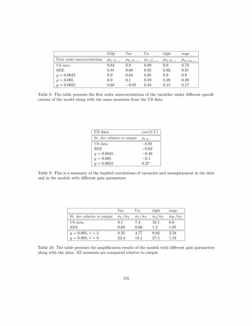
Gdp Vac Un tight wage

First order autocorrelations �Yt;Yt�1 �Vt;Vt�1 �Ut;Ut�1 �#t;#t�1 �wt;wt�1US data 0:84 0:9 0:89 0:9 0:73REE 0:91 0:68 0:95 0:92 0:91g = 0:0045 0:9 0:64 0:95 0:9 0:9g = 0:005 0:9 0:1 0:59 0:28 0:39g = 0:0055 0:68 �0:05 0:34 0:15 0:17

Table 8: The table presents the �rst order autocorrelations of the variables under di¤erent speci�-cations of the model along with the same moments from the US data

US data corr(V,U)

St. dev relative to output �v;u

US data �0:91REE �0:63g = 0:0045 �0:49g = 0:005 �0:1g = 0:0055 0:27

Table 9: This is a summary of the implied correlations of vacancies and unemployment in the dataand in the models with di¤erent gain parameters

Vac Un tight wage

St. dev relative to output �V =�Y �U=�Y �#=�Y �W =�Y

US data 9:1 7:4 16:1 0:6REE 0:68 0:66 1:2 1:05

g = 0:005, ` = 2 8:35 4:77 9:93 3:58g = 0:005, ` = 0 23:4 13:1 27:5 1:53

Table 10: The table presents the ampli�cation results of the models with di¤erent gain parametersalong with the data. All moments are computed relative to output

155

0 1 2 3 4 5 6 7­2

­1

0

1x 10 ­3

time

Une

mpl

oym

ent

0 1 2 3 4 5 6 70

1

2

3x 10 ­3

time

Vac

anci

es0 1 2 3 4 5 6 7

0

0.5

1

1.5x 10 ­3

time

Inco

me

0 1 2 3 4 5 6 70

2

4x 10 ­3

timeT

ight

ness

0 1 2 3 4 5 6 70

1

2x 10 ­3

time

Wag

e

0 1 2 3 4 5 6 7­5

0

5x 10 ­5

time

Hou

rs

0 1 2 3 4 5 6 70

0.5

1x 10 ­3

time

Con

sum

ptio

n

0 1 2 3 4 5 6 70

0.5

1

1.5x 10 ­3

time

Pro

duct

ivity

Figure 1: Those are impulse responses after a unit technology shock. The red solid line represents the ra-tional expectations equilibrium responses while the blue dashed lines the impulse responses under perpetuallearning. The gain parameter g is set to 0.0055

156

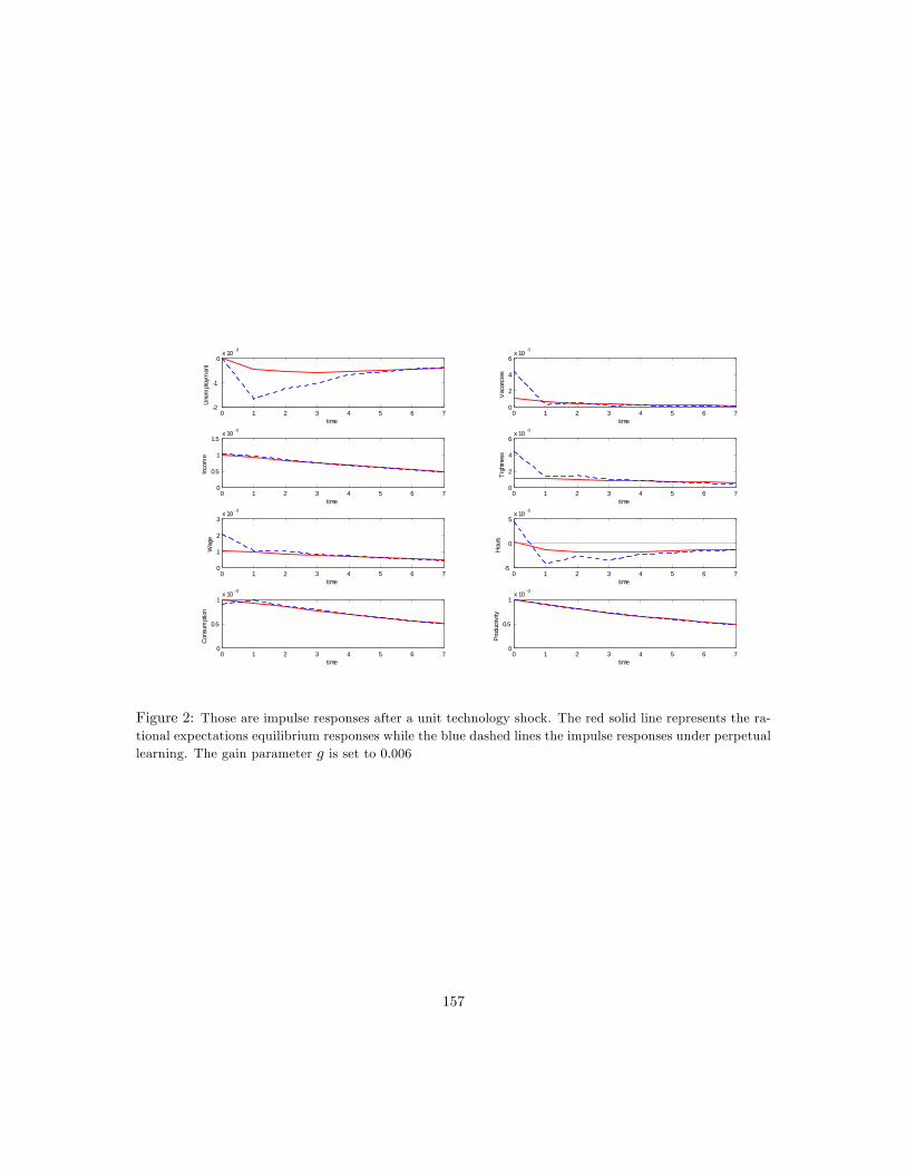
0 1 2 3 4 5 6 7­2

­1

0x 10 ­3

time

Une

mpl

oym

ent

0 1 2 3 4 5 6 70

2

4

6x 10 ­3

time

Vac

anci

es0 1 2 3 4 5 6 7

0

0.5

1

1.5x 10 ­3

time

Inco

me

0 1 2 3 4 5 6 70

2

4

6x 10 ­3

timeT

ight

ness

0 1 2 3 4 5 6 70

1

2

3x 10 ­3

time

Wag

e

0 1 2 3 4 5 6 7­5

0

5x 10 ­5

time

Hou

rs

0 1 2 3 4 5 6 70

0.5

1x 10 ­3

time

Con

sum

ptio

n

0 1 2 3 4 5 6 70

0.5

1x 10 ­3

time

Pro

duct

ivity

Figure 2: Those are impulse responses after a unit technology shock. The red solid line represents the ra-tional expectations equilibrium responses while the blue dashed lines the impulse responses under perpetuallearning. The gain parameter g is set to 0.006

157

0 1 2 3 4 5 6 70

0.5

1

1.5

2

2.5

3

3.5

4

4.5x 10 ­3

time

Vac

anci

es

g=0 (REE)g=0.005g=0.0055g=0.006

Figure 3: Responses of vacancies after a unit productivity shock. The solid red line is the responce in therational expectations model, the blue dashed line is the model with learning and constant gain parameter0.005. The black dotted responce corresponds to the learning model with gain parameter 0.0055 and thegreen dashed and dotted line to gain 0.006

158

Coe¢ cient mean median RE

g=0.005 g=0.005

�d0 0 0 0�k0 0 0 0�L0 0 0 0�r0 0 0 0�n0 0 0 0�d1 �37:9 �10:02 �13:74�k1 2:2 0:69 0:64�L1 �0:48 �0:53 �0:53�r1 �0:48 �0:44 �0:52�n1 0:47 0:38 0:37�d2 2:24 �0:11 �0:01�k2 0:27 0:40 0:41�L2 �0:003 0:002 0:002�r2 0:89 0:88 0:9�n2 0:02 0:02 0:03

Table 11: Those are the means and medians of the distributions of the belief coe¢ cients inducedby perpetual learning along with the rational expectations coe¢ cients.

159

02

000

400

06

000

800

01

000

0­202

x 1

0­4

Dividend

Inte

rce

pt

02

000

400

06

000

800

01

000

0­4

0

­200

Sta

te V

ari

abl

e 1

 (em

plo

ymen

t)

02

000

400

06

000

800

01

000

0­0

.50

0.51

Sta

te V

ari

abl

e 2

 (te

chn

olo

gy)

02

000

400

06

000

800

01

000

0­4­202

x 1

0­5

Vacancy cost

02

000

400

06

000

800

01

000

0­2024

02

000

400

06

000

800

01

000

00

.2

0.4

0.6

0.8

02

000

400

06

000

800

01

000

0­202

x 1

0­7

Labor Supply

02

000

400

06

000

800

01

000

0­0

.55

­0.5

­0.4

5

02

000

400

06

000

800

01

000

0­2024

x 1

0­3

02

000

400

06

000

800

01

000

0­1

0­505x

 10­5

Firm Demand

02

000

400

06

000

800

01

000

0­1

0­505

02

000

400

06

000

800

01

000

00

.51

1.5

02

000

400

06

000

800

01

000

0­2­101

x 1

0­6

Employment

02

000

400

06

000

800

01

000

00

.2

0.4

0.6

0.8

02

000

400

06

000

800

01

000

00

.01

0.0

2

0.0

3

0.0

4

Figure4:Thosearetheestimatesofthebeliefparameterswhenthelearning

modelissimulatedfor10000periodswitha

decreasinggaing t=1=t.Thered�atlinesaretherationalexpectationscoe¢cients.Theparametersareconvergingtothe

rationalbeliefsinthelongrun.

160

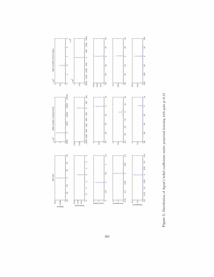
­60

­40

­20

020

4060

0

0.00

5

0.01

Dividend

Inte

rcep

t

­500

00

5000

1000

015

000

2000

0012

x 10

­3St

ate 

varia

ble 

1 (e

mpl

oym

ent)

­2­1

01

23

x 10

4

0

0.51

x 10

­4St

ate 

varia

ble 

2 (te

chno

logy

)

­4­3

­2­1

01

23

0

0.01

0.02

0.03

Vacancy cost

­120

0­1

000

­800

­600

­400

­200

020

040

00

0.02

0.04

­200

0­1

500

­100

0­5

000

500

1000

1500

0

0.51

x 10

­3

­1­0

.50

0.5

11.

5024

Labor Supply

­40

­30

­20

­10

010

0

0.51

­60

­40

­20

020

400

0.01

0.02

0.03

­0.1

5­0

.1­0

.05

00.

050.

1012

Firm Demand

­40

­30

­20

­10

010

200

0.51

­60

­40

­20

020

400

0.050.

1

­0.2

­0.1

5­0

.1­0

.05

00.

050.

10.

150

0.2

0.4

Employment

­80

­60

­40

­20

020

0

0.51

­150

­100

­50

050

100

0

0.01

0.02

Figure5:DistributionofAgent�sbeliefcoe¢cientsunderperpetuallearningwithgaing=0.15

161